Efficient interval estimation for age-adjusted cancer rates · EfÞcient interval estimation for...

Statistical Methods in Medical Research 2006; 15: 547–569

Efficient interval estimation for age-adjustedcancer ratesRam C Tiwari National Cancer Institute, NIH, Bethesda, MD, USA, Limin X Clegg Officeof Healthcare Inspections, OIG, Department of Veterans Affairs, Washington, DC, USA andZhaohui Zou Information Management Services, Inc., Silver Spring, MD, USA

The age-adjusted cancer rates are defined as the weighted average of the age-specific cancer rates, where theweights are positive, known, and normalized so that their sum is 1. Fay and Feuer developed a confidenceinterval for a single age-adjusted rate based on the gamma approximation. Fay used the gamma appro-ximations to construct an F interval for the ratio of two age-adjusted rates. Modifications of the gammaand F intervals are proposed and a simulation study is carried out to show that these modified gammaand modified F intervals are more efficient than the gamma and F intervals, respectively, in the sense thatthe proposed intervals have empirical coverage probabilities less than or equal to their counterparts, andthat they also retain the nominal level. The normal and beta confidence intervals for a single age-adjustedrate are also provided, but they are shown to be slightly liberal. Finally, for comparing two correlatedage-adjusted rates, the confidence intervals for the difference and for the ratio of the two age-adjusted ratesare derived incorporating the correlation between the two rates. The proposed gamma and F intervalsand the normal intervals for the correlated age-adjusted rates are recommended to be implemented in theSurveillance, Epidemiology and End Results Program of the National Cancer Institute.

1 Introduction

Despite rapid advances in medicine, cancer continues to be a major public health concernin the US and around the world. The total number of deaths due to cancer continuesto rise, even though the age-adjusted mortality rates for many common cancer sitescontinue to decline.1 Many public and private agencies dealing with cancer and relatedissues depend on these statistics for planning and resource allocation. Such figures haveimportant social and economic ramifications, from deciding which programs get funded,to deciding how funds are allocated among various programs. Having reliable and accu-rate confidence intervals (CIs) for the means of the age-adjusted cancer mortality andincidence rates for recent years is very important for everyone concerned. The higher thecoverage probabilities of the CIs, the more conservative the CIs are. Therefore, a desir-able property of these CIs is that while retaining the nominal level, they have coverageprobabilities as close to the nominal level as possible.

In the US, the data on cancer mortality are obtained from death certificates. Due toadministrative and procedural delays, these data become fully available to the public

Address for correspondence: Limin Clegg, Office of Healthcare Inspections, VA OIG 801 1 Street, NW,Room 1013, Washington, DC 20001, USA. E-mail: [email protected]

© 2006 SAGE Publications 10.1177/0962280206070621

548 RC Tiwari, LX Clegg and Z Zou

from the National Center for Health Statistics (NCHS) after approximately three years.The cancer incidence and mortality data are also available from the Surveillance,Epidemiology and End Results (SEER) Program of the National Cancer Institute(NCI). The SEER Program is an authoritative source for the cancer incidence and sur-vival data in the US Population data are available from the US Census Bureau. TheAmerican Cancer Society (ACS) publishes reports on cancer trends in their widely cir-culated annual publication,2 Cancer Facts & Figures, which is also available online:http://www.cancer.org/.

The state-level age-adjusted cancer (incidence or mortality) rates are given by

ri =J∑

j=1

wjdij

nij, i = 1, . . . , I

where dij and nij are the number of cancer (incidence or mortality) counts and the countof mid-year population for the age-group j and the state i, respectively, and the wj arethe normalized proportion of mid-year population for the age-group j in the standardpopulation, so that

∑Jj=1 wj = 1. In the SEER Program, for each of the 51 regions (50

states and Washington D.C.) in the US, there are 19 standard age-groups consisting of0−<1, 1−4, 5−9, . . . , 85+. The US-level age-adjusted cancer (incidence or mortality)rates are given by

r =J∑

j=1

wjdj

nj

with dj = ∑Ii=1 dij and nj = ∑I

i=1 nij. The SEER Program contains age-adjusted mor-tality rates, based on the 2000 US standard population, for the US and for each of the51 regions by cancer sites. The age-adjusted mortality rates for a selected number ofcancer sites and a number of countries in the world are also reported in the CancerFacts & Figures publication.2 These age-adjusted rates are based on the World HealthOrganization’s world standard population. Thus, the results of this paper, even thoughdiscussed in the context of the age-adjusted mortality rates for the US, apply to similardata sets for other countries.

For each i (i = 1, . . . , I), let d(−i)j = dj − dij and n(−i)j = nj − nij and define

r(−i) =J∑

j=1

wjd(−i)j

n(−i)j

to be the age-adjusted rate for the rest of the US after deleting the region i.Let Dij, Dj, D(−i)j, Ri, R(−i) and R denote the random variables whose realiza-

tions are dij, dj, d(−i)j, ri, r(−i) and r, respectively. We assume that Dij are independentPoisson random variables3 with parameters λij, that is, Dij ∼ind Po(nijλij). Note that by

Efficient interval estimation for age-adjusted cancer rates 549

the moment generating function, D(−i)j ∼ Po(∑I

i′ �=i ni′jλi′j) and Dj ∼ Po(∑I

i=1 nijλij).

Let ξij = nij/nj, ξ(−i)j = ∑Ii′ �=i ξi′j and ξj = nj/n, where n = ∑J

j=1 nj = ∑Ii=1∑J

j=1 nij.Let µi, µ(−i), µ, vi = σ 2

i /n, ν(−i) = σ 2(−i)/n and v ≡ σ 2/n be the means and variances

of Ri, R(−i) and R, respectively, and let and ρi/n be the Cov(Ri, R), where their explicitexpressions are derived in Appendix A. Let wij = wj/nij and define the estimates of µi,µ(−i), µ, σ 2

i , σ 2(−i), σ 2 and ρi as

µi = ri; µ(−i) = r(−i); µ = r

σ 2i = n

J∑

j=1

w2ijdij; σ 2

(−i) = nJ∑

j=1

w2j

d(−j)

n2(−j)

σ 2 = nJ∑

j=1

w2j

dj

n2j

; ρi = nJ∑

j=1

wijwj

njdij

For a rare cancer site, as the observed total counts di are very small with dij = 0 plausiblyfor several j, the value of ri is either close to 0 or equal to 0. As we will see subse-quently, when ri = 0, the gamma intervals of Fay and Feuer4 is not defined. To avoidsuch situations, we introduce a correction factor, which amounts to distributing a countof 1 uniformly to all J categories, and hence adding 1/J, the expected value under multi-nomial distribution with parameters 1 and cell probabilities 1/J, to dij, j = 1, . . . , J, incalculation of the estimates of µi, σ 2

i and ρi. We redefine ri as

ri =J∑

j=1

wij

(dij + 1

J

)= ri + wi

where wi = 1/J∑J

j=1 wij and modify the estimates of µi, σ 2i , σ 2

(−i) and ρi accordinglyby replacing dij by (dij + 1/J). Thus,

µi = ri; σ 2i = n

J∑

j=1

w2ij

(dij + 1

J

); ρi = n

J∑

j=1

wijwj

nj

(dij + 1

J

)

Note that ri ≈ ri for common cancer sites as wi ≈ 0. Let

νi = σ 2i

n; νi = σ 2

i

n; ν = σ 2

n

The objectives of this paper include the construction of CIs for parameters such asi) the mean µi of the age-adjusted rate for the region i; ii) the mean µ of the age-adjusted


rate for the US; iii) the ratio of the mean age-adjusted rates µi/µi′ for region i to regioni′; iv) the ratio of the mean age-adjusted rates µi/µ(−i) for region i to the rest of the US;v) the ratio of the mean age-adjusted rates µi/µ for region i to the US; and vi) thedifference of the mean age-adjusted rates µi − µ, between region i and the US. Fay andFeuer4 derived a CI for µi (or µ) assuming that a mixture of Poisson distributions can beapproximated by a gamma distribution and compared the performance of the gammaintervals with the approximate bootstrap confidence (ABC) intervals5−7 and the ‘chi-squared’ intervals of Dobson et al.8 through simulations. They observed that the gammaintervals retained at least the nominal coverage and were more conservative than the ABCintervals and chi-squared intervals. We propose a modification of the gamma intervalfor µi (or µ) developed by Fay and Feuer4 and derive new CIs for µi (and µ) based onthe beta and normal approximations of Ri (and R).

Fay9 used the gamma approximation of Fay and Feuer4 and developed a CI, based onan approximate F distribution, for the ratio of two age-adjusted rates that can be appliedto µi/µi′ and µi/µ(−i), but not to µi/µ as the age-adjusted rate for the US involves thecounts from the region i. We also propose a modification of the F interval of Fay9. We usethe normal approximations of Ri/Ri′ , Ri/R(−i), Ri/R and Ri − R, taking into accountthe correlation between Ri and R, and construct the CIs for µi/µi′ , µi/µ(−i), µi/µ andµi − µ. It is important to mention that for comparing the state and US level age-adjustedrates, the current procedure10 is to use the normal CI for µi − µ based on ρi = 0. Forsimulations, we use the observed age-adjusted mortality rates for the 51 regions and theUS for year 2002 from the SEER Program for a rare cancer site, the tongue cancer.

The rest of the paper is organized as follows. In Section 3, we briefly review the worksof Fay and Feuer4 and Fay9 and present the modified gamma and F intervals. We alsoderive the CIs for the ratio of the means of the two age-adjusted rates namely the age-adjusted rates of any two regions, any region to the rest of the country, any region tothe entire country and for the difference of the means of the age-adjusted rates betweena region and the country. Simulations are carried out in Section 4, and we discuss ourfindings in Section 5. The conclusions are presented in Section 6.

2 Confidence intervals for age-adjusted rates

2.1 Gamma and F approximationsNote that if X ∼ Po(θ), then for an integer x ≥ 0,

P(X ≥ x|θ) =∫ θ

0fZ(z|x, 1) dz

where Z ∼ G(x, 1) =d 1/2χ22x and, in general, G(α, β) =d β/2χ2

2α (allowing non-integer degrees of freedom) has density

fZ(x|α, β) = 1βα�(α)

exp(

− xβ

)xα−1, x > 0


with mean E(Z) = αβ and variance Var(Z) = αβ2. Let x be the observed value of Xand let (L(x; α), U(x, α)) denote the 100(1 − α)% CI for θ , where L(x; α) is obtainedby solving the equation

P(X ≥ x|θ = L(x; α)) = α

2

and U(x, α) is obtained by solving

P(X ≤ x|θ = U(x; α)) = α

2

or equivalently by solving

P(X > x|θ = U(x; α)) = P(X ≥ x + 1|θ = U(x; α)) = 1 − α

2

Thus, L(x; α) = 1/2(χ22x)

−1(α/2) and U(x; α) = 1/2(χ22(x+1))

−1(1 − α/2). Fay andFeuer4 called the interval (L(x; α), U(x; α)) ‘exact’ while others, for example, Johnsonand Kotz,11 use the term ‘approximate’ interval.

Let wi(1) ≤ · · · ≤ wi(J) be the ordered values of wij, j = 1, . . . , J. Fay and Feuer4

assumed that a mixture of Poisson distributions is approximately distributed as a gammadistribution; that is,

P

J∑

j=1

wijDij ≥ y|µi, νi

≈∫ µi

0fZi

(z∣∣∣∣y2

νi,νi

y

)dz

where Zi ∼ G(y2/νi, νi/y). This assumption essentially means that the distribution ofa linear combination of independent Poisson random variables is approximately dis-tributed as a gamma random variable with the mean and variance of the gammadistribution equal to the mean and variance of the linear combination, respectively.Fay and Feuer4 used this approximation to construct approximate 100(1 − α)% CIs forthe true age-adjusted rates µi.

The lower confidence limit L(ri; α) was obtained by solving the equation

α

2= P

J∑

j=1

wijDij ≥ ri|µi, νi

≈∫ L(µi;νi)

0fZi

(z∣∣∣∣r2

i

νi,νi

ri

)dz

This yields

L(ri; νi; α) = G−1

(α

2;

r2i

νi,νi

ri

)= νi

2ri

(χ2

2r2i /νi

)−1 (α

2

)

where G−1 is the inverse function of the gamma distribution function and (χ2l )−1(α)

denotes the 100αth percentile of the chi-squared distribution with l degrees of freedom.


Note that when ri = 0, L(ri; νi; α) is not defined. For the upper confidence limit U(ri; α),Fay and Feuer4 solved the equation

1 − α

2= P

J∑

j=1

wijDij > ri|µi, νi

≥ P

J∑

j=1

wijDij ≥ ri + wi(J)|µi, νi

≈∫ U(µi;νi)

0fZi

(z∣∣∣∣(ri + wi(J))

2

νi + w2i(J)

,νi + w2

i(J)

ri + wi(J)

)dz

resulting in

U(ri; νi, wi(J); α) = G−1

(1 − α

2;

r2i

νi,νi

ri, wi(J)

)

= νi + w2i(J)

2(ri + wi(J))

(χ2

(2(ri+wi(J))2/νi+w2

i(J))

)−1(

1 − α

2

)

Fay and Feuer4 performed simulations to study the performance of their gamma CIs(L(ri; νi; α), U(ri; νi; wi(J); α)) and found that the upper confidence limits were moreconservative than those based on the ABC intervals5−7 and the chi-squared intervals ofDobson et al.,8 henceforth referred to as DKES intervals. For completeness the ABC andDKES intervals are given in Appendix B.

Fay and Feuer4 have mentioned that when the weights wij for all j are equal to a con-stant, ci > 0, say, the CI for µi = E(

∑Jj=1 wijDij) = ciE(Di) is (ciL(di; α), ciU(di : α))

exact with Di ∼ Po(∑J

j=1 nijλij). However, note that since wij = wj/nij depend on boththe standards wj and on the mid-year populations nij, the condition that wij are equalto a constant for all j is not easily satisfied. For example, a sufficient condition for thiscondition to hold is that wj are all equal and nij are all equal. Another sufficient con-dition for wij to be equal to a constant for all j is to assume nij is proportional to wj,independent of i, for all j. If a populous state like California or New York has the age-group distribution of its population similar to that of the entire US, then for that state,one may expect nij to be proportional to wj and hence the CI for µi to be exact.

Since wi(l) ≤ wi(l+1), we have

P

J∑

j=1


≥ P

J∑

j=1

wijDij ≥ ri + wi(l)|µi, νi

≥ P

J∑

j=1

wijDij ≥ ri + wi(l+1)|µi, νi

, l = 1, . . . , J − 1


Thus proceeding as above, one can construct the upper confidence limitsU(ri; νi; wi(1); α), U(ri; νi; wi(2); α), . . . , U(ri; νi, wi(J); α) varying from being the mostliberal upper limit to the most conservative upper limit. In fact, there are an infinitenumber of choices for such an upper confidence limit.

As a compromise, we propose an upper limit that is based on the mean wi =1/J

∑Jj=1 wij and that depends on all wi(l), l = 1, . . . , J. As mentioned earlier, this

assumes distributing a count of 1 uniformly to all J age-groups. Thus,

1 − α

2= P

J∑

j=1


≥ P

J∑

j=1

wijDij ≥ ri + wi|µi, νi

= P

J∑

j=1

wijDij ≥ ri|µi, νi

Now, assuming that (dij + 1/J)have means equal to their variances, similar to the Poissondistribution, so that

Var

J∑

j=1

wij

(dij + 1

J

)

=J∑

j=1

w2ij

(dij + 1

J

)

using the gamma approximation, the upper confidence limit for µi is given by

U(ri; νi; wi; α) = νi

2ri(χ2

(2r2i /νi)

)−1(

1 − α

2

)

Therefore, the proposed gamma CI for µi is (L(ri; νi; α), U(ri; νi; wi; α)). Anotherapproximation of the upper confidence limit based on the mean wi can be obtainedby using (νi + w2

i ) instead of νi. This results in the following CI: (L(ri; νi; α), U(ri; νi +w2

i ; wi; α)). Through simulations (not shown here), we found that these two intervalsperformed very similarly. Therefore, we will focus only on (L(ri; νi; α), U(ri; νi; wi; α)).Note that the lower limits of the gamma interval of Fay and Feuer4 and the modi-fied gamma intervals are the same. We shall define the CI for µi when ri = 0 as (0,U(ri; νi; wi; α)), thus ensuring a coverage probability of at least (1 − α).

Fay9 developed a confidence interval for the ratio of two age-adjusted rates, µi/µi′ , forµi, µi′ > 0, based on Ri = ∑J

j=1 wijDij and Ri′ = ∑Jj=1 wi′jDi′j, where Dij and Di′j are

independent. Assuming the gamma approximations for Ri and Ri′ , Fay9 used the resultthat, conditional on Dij + Di′j = tj, the distribution of Dij is a binomial distribution withparameters tj and nij(λij/λi′j)/nij(λij/λi′j) + ni′j. For constructing the lower confidencelimit for µi/µi′ , Fay9 assumed that µi is distributed as gamma with mean ri and variance


νi and that µi′ is distributed as gamma with mean (ri′ + Wi′) and variance (νi′ + W2i′)

and used the result that, conditional on tj,(

ri′ + Wi′

ri

)µi

µi′∼ F((2r2

i /νi),(2(ri′+Wi′ )2/(νi′+W2i′ )))

where Wi′ = maxj:di′j<tj{wi′j} and for independent χ2m =d G(m/2, 2) and χ2

n =d

G(n/2, 2), F(m,n) =d (χ2m/m)/(χ2

n/n) denotes the F distribution with numerator degreesof freedom (d.f.) m and the denominator d.f. n with density given by

g(x|m, n) = �((m + n)/2)

�(m/2)�(n/2)

(mn

)m/2 x(m/2)−1

(1 + (m/n)x)(m+n)/2 , 0 < x < ∞

Since the numerator and the denominator chi-squared random variables inF((2r2

i )/νi),(2(ri′+Wi′ )2/(νi′+W2i′ ))

depend on tj, the unconditional distribution of µi/µi′ isa mixture of F distributions, and not an F distribution.

The lower confidence limit isri

ri′ + Wi′F−1

((2r2i )/νi,(2(ri′+Wi′ )2)/(νi′+W2

i′ ))

(α

2

)

where F−1(a,b)

(p) is the pth percentile of F(a,b). Now, assuming that µi is distributed asgamma with mean (ri + Wi) and variance (νi + W2

i ) and that µi′ is distributed as gammawith mean ri′ and variance νi′ , Fay9 derived the upper confidence limit to be

ri + Wi

ri′F−1

((2(ri+Wi)2)/(νi+W2i ),(2r2

i′ )/ν′i ))

(1 − α

2

)

Note that this approximation cannot be readily applied for constructing CIs for the ratiosµi/µ, that is, the ratios of the age-adjusted rates for the regions i to the US age-adjustedrates, as the latter depends on the former ones.

We propose a modification in the above CI for µi/µi′ . For the lower limit, we assumethat µi is distributed as gamma with mean ri and variance νi and that µi′ is distributedas gamma with mean ri′ and variance νi′ and since the two distributions are independentchi-squares, we have (

ri′

ri

)µi

µi′∼ F((2r2

i )/νi,(2r2i′ )/νi′ )

This results in the lower limit to be ri/ri′ F−1((2r2

i )/νi,(2r2i′ )/νi′ )

(α/2). Similarly, the upper limit

can be obtained. The proposed CI for µi/µi′ is(

ri

ri′F−1

((2r2i )/νi,(2r2

i′ )/νi′ )

(α

2

),

ri

ri′F−1

((2r2i )/νi,(2r2

i′ )/νi′ )

(1 − α

2

))


Another CI for µi/µi′ using (ri + wi) and (νi + w2i ) instead of ri and νi is given by

(ri

ri′ + wi′F−1

((2r2i )/νi,(2(ri′+wi′ )2)/(νi′+w2

i′ ))

(α

2

),

ri + wi

ri′F−1

((2(ri+wi)2)/(νi+w2i ),(2r2

i′ )/ν′i )

(1 − α

2

))

Once again, we mention that this interval performs similarly to the above one, and wewill not focus on this. We further remark that, unlike as in Fay,9 these intervals do notassume the dependence of the wij on tj.

2.2 Normal approximationsDefine Rij = Dij/nij(= Dij/(nξijξj)). Let n → ∞ so that 0 < ξij, ξj < 1. Note that

0 < λij < ∞. Then as min{nijλij} → ∞,

√n(

ξijξj

λij

)1/2

(Rij − λij) −→ind N(0, 1), i = 1, . . . , I; j = 1, . . . , J

That is, Rij are independent and asymptotically normally distributed, Rij ∼AN(λij, λij/(nξijξj)). The other asymptotic results based on Rij, 100(1 − α)% CIs forµi, µ, µi/µi′ , µi/µ, µi/µ(−i) and µi − µ, and their logarithmic and logit transforma-tions are presented in Appendix C. In particular, the 100(1 − α)% CIs for µi/µ, andµi − µ, based on the correlated age-adjusted rates, are given by

µi

µ=

µi

µ± zα/2

√(σ 2

i µ2 + σ 2µ2i − 2ρiµiµ)

√nµ4

∨ 0

µi − µ = µi − µ ± zα/2

√σ 2

i + σ 2 − 2ρi√n

where a ∨ b = max(a, b). When ρi = 0, which is true iff λij = 0 for all j, these CIs reduceto (see, e.g., Ries et al.10 for the CI of µi − µ when ρi = 0)

µi

µ={

µi

µ± zα/2

1√n

√1µ4 (σ 2

i µ2 + σ 2µ2i )

}∨ 0, µi − µ = µi − µ ± zα/2

√σ 2

i + σ 2

√n

Since ρi > 0, the length of the CI for µi − µ, ignoring the adjustment for ρi, is wider,and hence the interval is more conservative.

2.3 Beta approximationsIn general, the age-adjusted rates are less than 1 and equal to 1 if and only if there is

one age-group with both the values of cancer counts and population at risk for that age


group equal to 1, which is not a practical case. A rationale for the beta approximationis as follows. Let Ri = ∑J

j=1 wjRij, where Rij = Dij/nij. Let Dij and Dij be independentPoisson random variables with means nijλij and nij(1 − λij), respectively. Then the dis-tribution of Dij|Dij+Dij=nij,λij

∼ Bin(nij, λij), a binomial distribution with parameters nij

and λij.12 Using the result, given in Appendix D, we can approximate the distribution ofRi by a beta distribution with parameters ai and bi, Be(ai, bi), where

ai = ri

(ri(1 − ri)

νi− 1

), bi = (1 − ri)

(ri(1 − ri)

νi− 1

)

We define an approximate 100(1 − α)% CI for µi as (LRi, URi

), where LR and UR areobtained by solving the following incomplete beta integrals:

∫ LRi

0B(x|ai, bi) dx = α

2,∫ URi

0B(x|ai, bi) dx = 1 − α

2

Here, B(x|a, b) is the density of a beta distribution, Be(a, b), with parameters a and b.

3 Examples and simulations

As an illustration, age-adjusted tongue cancer mortality rates were calculated for eachof the regions. Tongue cancer occurs mostly among the elders. The 2002 mortalitydata for tongue cancer, even though available from the NCHS, were obtained fromthe SEER Program of the NCI (see the web site: www.seer.cancer.gov). We carried outtwo different simulation studies to evaluate the performance of the proposed gamma,beta and normal (with lower limits truncated at 0) intervals with the gamma intervalof Fay and Feuer.4 In the first simulation study, we took the true means of the Poissondistributions of Dij to be the observed values of deaths in the (i, j)th cell, where i standsfor the 51 regions of the US (50 states and Washington DC) and j stands for the 19age-groups, to be (i = 1, . . . , 51; j = 1, . . . , 19). Therefore, the true value of µi is theobserved value of the age-adjusted rate for each i. From the Poisson distributions, wegenerated 10 000 values of dij, and obtained the observed values of the age-adjustedrates Ri using the normalized weights wj, based on the 2000 US standard population,so that

∑Jj=1 wj = 1. We computed approximate 95% CIs for µi for each of the 51

regions using the gamma intervals of Fay and Feuer4 and the proposed gamma, beta andnormal intervals. Additionally, we compared the F interval of Fay9 for µi/µ(−i) with theproposed F and normal intervals (with left limits truncated at 0). We compared the age-adjusted rate of each of the 51 regions with the rest of US age-adjusted rate. Once again,we chose the year 2002 tongue cancer mortality age-adjusted rates for the 51 regions.The simulations were carried out assuming the 2000 standard population generating dijfrom independent Poisson with mean equal to the observed dij.


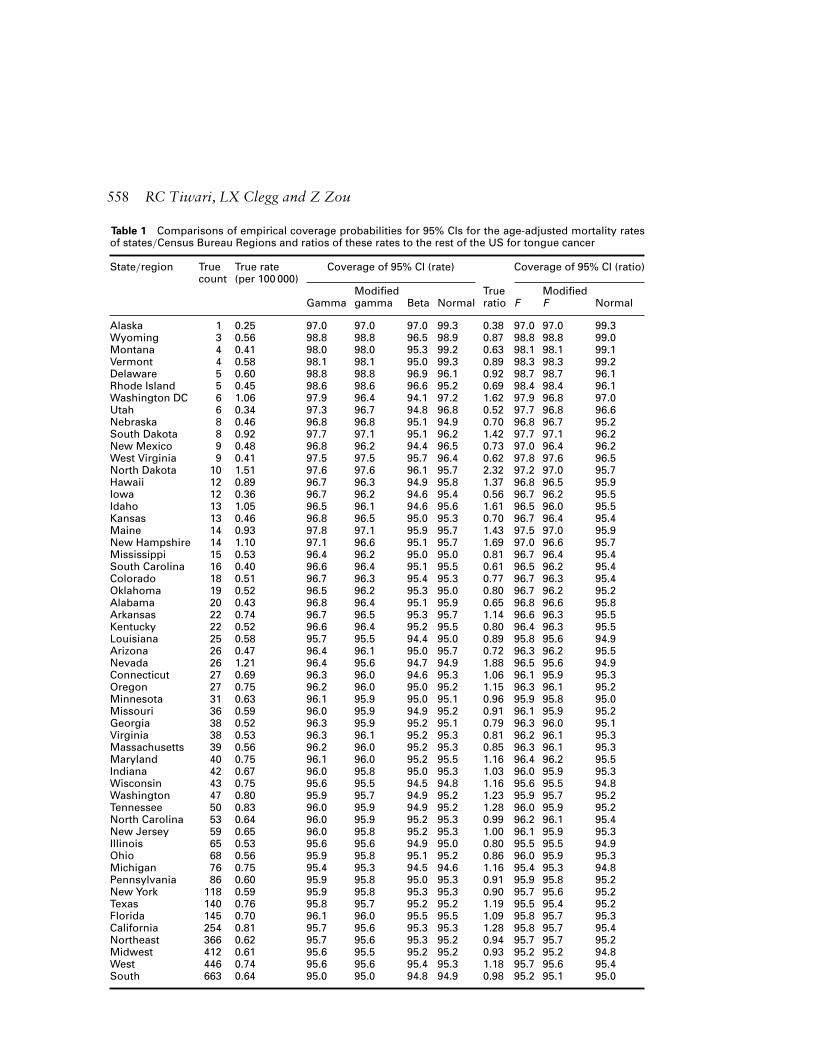
Table 1 gives the results of the first simulation study. Columns 2 and 3 of the tablegive the observed (true) tongue cancer mortality counts and age-adjusted rates (per100 000 mid-year population) for the 50 states, the District of Columbia, and the fourCensus Bureau Regions (Northwest, Midwest, West, and South). Column 3 presents theempirical coverage probabilities of the 95% CIs for the (simulated) age-adjusted ratesbased on the gamma, modified gamma, beta, and normal approximations. Column 5shows the observed (true) ratios of age-adjusted rates of each of the 51 regions with therest of the US Column 6 gives the empirical coverage probabilities of the 95% CIs forthe (simulated) rate ratios based on F modified F and normal approximations.

Both the modified gamma and modified F intervals are more efficient than their coun-terparts because their empirical coverage probabilities are at least 95%, but are lowerthan for the gamma and the F intervals. The beta and normal intervals are slightly liberalas they do not perform well as they have empirical coverage probabilities less than 95%for a number of regions.

In the second simulation study, we considered the effect of randomly generated valuesof wij and dij on the performance of the gamma, beta and normal intervals. Here, thesubscript i does not play any role, and is treated as a dummy variable, but it is kept for thesake of notational consistency. We generated 19 numbers, corresponding to the J = 19age-groups, from the uniform U(0, 1) distribution and standardized them (and calledthem wij; j = 1, . . . , 19) so that

∑19j=1 wij is a very small number, say, equal to 5.0 × 10−6.

We again generated 19 numbers from U(0, 1) and standardized them (and called themdij; j = 1, . . . , 19) so that their sum is small,

∑19j=1 dij = 20 . These standardized numbers

were taken to be the values of the true means λij, j = 1, . . . , 19.Then, we simulated 10 000 values of dij from the Poisson distributions with means

λij, j = 1, . . . , 19. From these, we calculated the age-adjusted rates ri and the 95% CIsfor µi using the gamma and normal intervals. We also calculated the variance of wij.We repeated the entire process 500 times. Note that we could have standardized the sum∑19

j=1 wij to any other small number, but we chose it to be 5.0 × 10−6 so that it wassimilar to what we have based on the 2000 US standard population and the 2002 age-adjusted rates. We also could have standardized the sum

∑19j=1 dij to any other number

than 20 possibly to 50, but we kept it to 20 to see the effect of small sample size; that is,the small number of total mortality counts for the region, i.

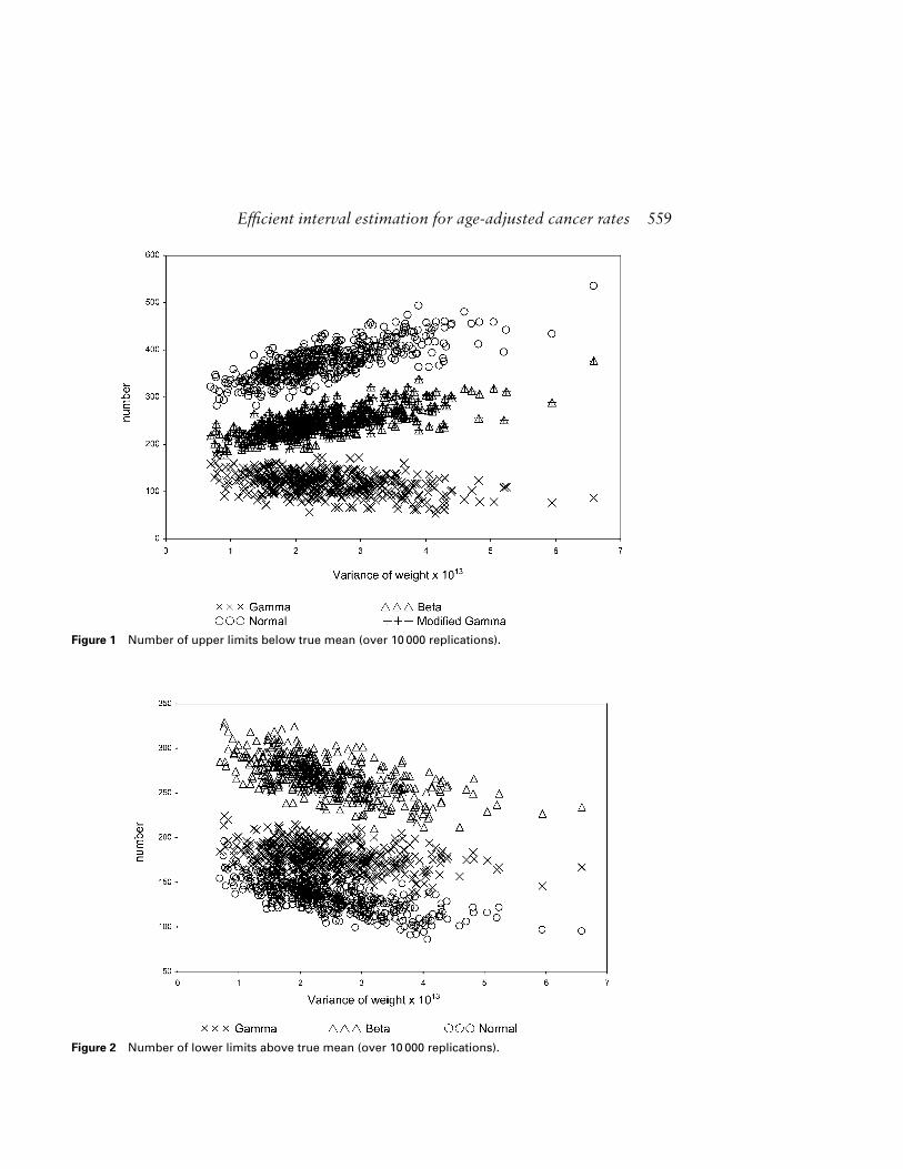
Note that out of 10 000 intervals, corresponding to each one of the 500 replications, itis expected that approximately 9500 intervals would contain the true mean µi and 500would not; that is, it is expected that approximately 250 values of the lower limits wouldbe above the true mean µi and about the same number of the upper limits would be belowthe true mean µi. In Figures 1 and 2, we plotted the 500 values of the variance of thenormalized weights wij on the x-axis, and the frequencies of the lower and upper limits ofµi for the Fay and Feuer4 intervals, modified gamma, beta and normal intervals that fell,respectively, above and below the true mean µi, were plotted on the y-axis. In Figure 3,we plotted both the lower and the upper limits against the variance of wij. Note thatthe two solid lines in Figure 3 correspond to the lower and upper 95% confidence limitsfor true proportion, p, based on Bin(10 000, 0.05), and then rescaled by multiplying by10 000; that is 10 000(0.05 ± 1.96

√0.05 × 0.95/10000) ≈ (457, 543). Thus the expected


Table 1 Comparisons of empirical coverage probabilities for 95% CIs for the age-adjusted mortality ratesof states/Census Bureau Regions and ratios of these rates to the rest of the US for tongue cancer

State/region True True rate Coverage of 95% CI (rate) Coverage of 95% CI (ratio)count (per 100 000)

Modified True ModifiedGamma gamma Beta Normal ratio F F Normal

Alaska 1 0.25 97.0 97.0 97.0 99.3 0.38 97.0 97.0 99.3Wyoming 3 0.56 98.8 98.8 96.5 98.9 0.87 98.8 98.8 99.0Montana 4 0.41 98.0 98.0 95.3 99.2 0.63 98.1 98.1 99.1Vermont 4 0.58 98.1 98.1 95.0 99.3 0.89 98.3 98.3 99.2Delaware 5 0.60 98.8 98.8 96.9 96.1 0.92 98.7 98.7 96.1Rhode Island 5 0.45 98.6 98.6 96.6 95.2 0.69 98.4 98.4 96.1Washington DC 6 1.06 97.9 96.4 94.1 97.2 1.62 97.9 96.8 97.0Utah 6 0.34 97.3 96.7 94.8 96.8 0.52 97.7 96.8 96.6Nebraska 8 0.46 96.8 96.8 95.1 94.9 0.70 96.8 96.7 95.2South Dakota 8 0.92 97.7 97.1 95.1 96.2 1.42 97.7 97.1 96.2New Mexico 9 0.48 96.8 96.2 94.4 96.5 0.73 97.0 96.4 96.2West Virginia 9 0.41 97.5 97.5 95.7 96.4 0.62 97.8 97.6 96.5North Dakota 10 1.51 97.6 97.6 96.1 95.7 2.32 97.2 97.0 95.7Hawaii 12 0.89 96.7 96.3 94.9 95.8 1.37 96.8 96.5 95.9Iowa 12 0.36 96.7 96.2 94.6 95.4 0.56 96.7 96.2 95.5Idaho 13 1.05 96.5 96.1 94.6 95.6 1.61 96.5 96.0 95.5Kansas 13 0.46 96.8 96.5 95.0 95.3 0.70 96.7 96.4 95.4Maine 14 0.93 97.8 97.1 95.9 95.7 1.43 97.5 97.0 95.9New Hampshire 14 1.10 97.1 96.6 95.1 95.7 1.69 97.0 96.6 95.7Mississippi 15 0.53 96.4 96.2 95.0 95.0 0.81 96.7 96.4 95.4South Carolina 16 0.40 96.6 96.4 95.1 95.5 0.61 96.5 96.2 95.4Colorado 18 0.51 96.7 96.3 95.4 95.3 0.77 96.7 96.3 95.4Oklahoma 19 0.52 96.5 96.2 95.3 95.0 0.80 96.7 96.2 95.2Alabama 20 0.43 96.8 96.4 95.1 95.9 0.65 96.8 96.6 95.8Arkansas 22 0.74 96.7 96.5 95.3 95.7 1.14 96.6 96.3 95.5Kentucky 22 0.52 96.6 96.4 95.2 95.5 0.80 96.4 96.3 95.5Louisiana 25 0.58 95.7 95.5 94.4 95.0 0.89 95.8 95.6 94.9Arizona 26 0.47 96.4 96.1 95.0 95.7 0.72 96.3 96.2 95.5Nevada 26 1.21 96.4 95.6 94.7 94.9 1.88 96.5 95.6 94.9Connecticut 27 0.69 96.3 96.0 94.6 95.3 1.06 96.1 95.9 95.3Oregon 27 0.75 96.2 96.0 95.0 95.2 1.15 96.3 96.1 95.2Minnesota 31 0.63 96.1 95.9 95.0 95.1 0.96 95.9 95.8 95.0Missouri 36 0.59 96.0 95.9 94.9 95.2 0.91 96.1 95.9 95.2Georgia 38 0.52 96.3 95.9 95.2 95.1 0.79 96.3 96.0 95.1Virginia 38 0.53 96.3 96.1 95.2 95.3 0.81 96.2 96.1 95.3Massachusetts 39 0.56 96.2 96.0 95.2 95.3 0.85 96.3 96.1 95.3Maryland 40 0.75 96.1 96.0 95.2 95.5 1.16 96.4 96.2 95.5Indiana 42 0.67 96.0 95.8 95.0 95.3 1.03 96.0 95.9 95.3Wisconsin 43 0.75 95.6 95.5 94.5 94.8 1.16 95.6 95.5 94.8Washington 47 0.80 95.9 95.7 94.9 95.2 1.23 95.9 95.7 95.2Tennessee 50 0.83 96.0 95.9 94.9 95.2 1.28 96.0 95.9 95.2North Carolina 53 0.64 96.0 95.9 95.2 95.3 0.99 96.2 96.1 95.4New Jersey 59 0.65 96.0 95.8 95.2 95.3 1.00 96.1 95.9 95.3Illinois 65 0.53 95.6 95.6 94.9 95.0 0.80 95.5 95.5 94.9Ohio 68 0.56 95.9 95.8 95.1 95.2 0.86 96.0 95.9 95.3Michigan 76 0.75 95.4 95.3 94.5 94.6 1.16 95.4 95.3 94.8Pennsylvania 86 0.60 95.9 95.8 95.0 95.3 0.91 95.9 95.8 95.2New York 118 0.59 95.9 95.8 95.3 95.3 0.90 95.7 95.6 95.2Texas 140 0.76 95.8 95.7 95.2 95.2 1.19 95.5 95.4 95.2Florida 145 0.70 96.1 96.0 95.5 95.5 1.09 95.8 95.7 95.3California 254 0.81 95.7 95.6 95.3 95.3 1.28 95.8 95.7 95.4Northeast 366 0.62 95.7 95.6 95.3 95.2 0.94 95.7 95.7 95.2Midwest 412 0.61 95.6 95.5 95.2 95.2 0.93 95.2 95.2 94.8West 446 0.74 95.6 95.6 95.4 95.3 1.18 95.7 95.6 95.4South 663 0.64 95.0 95.0 94.8 94.9 0.98 95.2 95.1 95.0


Figure 1 Number of upper limits below true mean (over 10 000 replications).

Figure 2 Number of lower limits above true mean (over 10 000 replications).


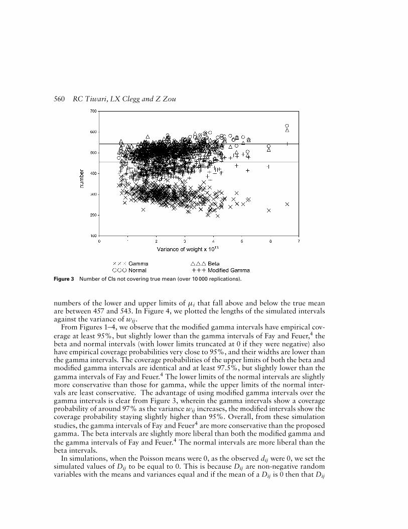
Figure 3 Number of CIs not covering true mean (over 10 000 replications).

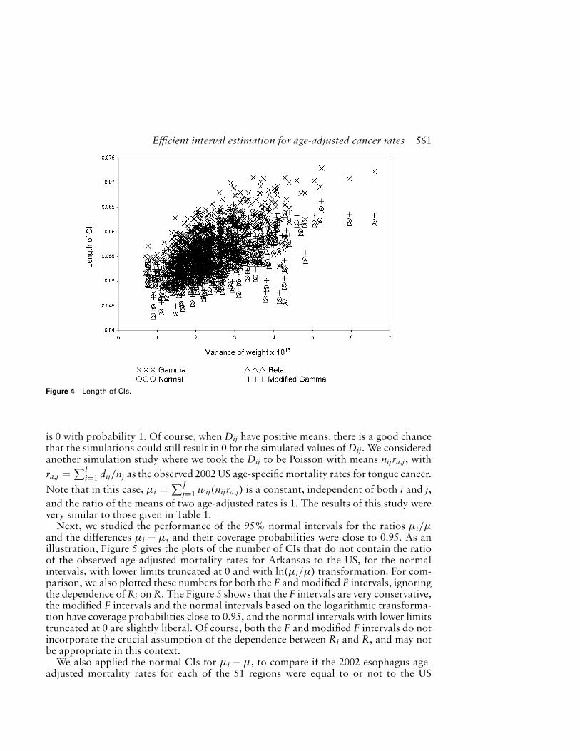
numbers of the lower and upper limits of µi that fall above and below the true meanare between 457 and 543. In Figure 4, we plotted the lengths of the simulated intervalsagainst the variance of wij.

From Figures 1–4, we observe that the modified gamma intervals have empirical cov-erage at least 95%, but slightly lower than the gamma intervals of Fay and Feuer,4 thebeta and normal intervals (with lower limits truncated at 0 if they were negative) alsohave empirical coverage probabilities very close to 95%, and their widths are lower thanthe gamma intervals. The coverage probabilities of the upper limits of both the beta andmodified gamma intervals are identical and at least 97.5%, but slightly lower than thegamma intervals of Fay and Feuer.4 The lower limits of the normal intervals are slightlymore conservative than those for gamma, while the upper limits of the normal inter-vals are least conservative. The advantage of using modified gamma intervals over thegamma intervals is clear from Figure 3, wherein the gamma intervals show a coverageprobability of around 97% as the variance wij increases, the modified intervals show thecoverage probability staying slightly higher than 95%. Overall, from these simulationstudies, the gamma intervals of Fay and Feuer4 are more conservative than the proposedgamma. The beta intervals are slightly more liberal than both the modified gamma andthe gamma intervals of Fay and Feuer.4 The normal intervals are more liberal than thebeta intervals.

In simulations, when the Poisson means were 0, as the observed dij were 0, we set thesimulated values of Dij to be equal to 0. This is because Dij are non-negative randomvariables with the means and variances equal and if the mean of a Dij is 0 then that Dij


Figure 4 Length of CIs.

is 0 with probability 1. Of course, when Dij have positive means, there is a good chancethat the simulations could still result in 0 for the simulated values of Dij. We consideredanother simulation study where we took the Dij to be Poisson with means nijra,j, withra,j = ∑I

i=1 dij/nj as the observed 2002 US age-specific mortality rates for tongue cancer.Note that in this case, µi = ∑J

j=1 wij(nijra,j) is a constant, independent of both i and j,and the ratio of the means of two age-adjusted rates is 1. The results of this study werevery similar to those given in Table 1.

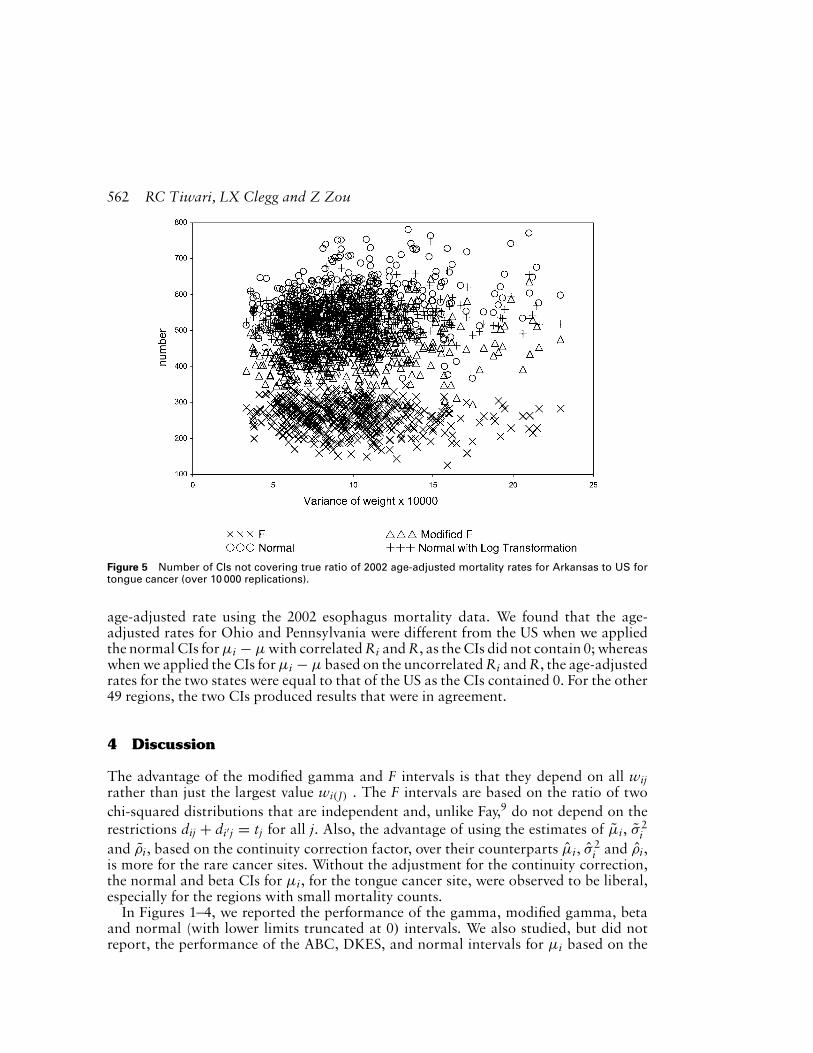
Next, we studied the performance of the 95% normal intervals for the ratios µi/µand the differences µi − µ, and their coverage probabilities were close to 0.95. As anillustration, Figure 5 gives the plots of the number of CIs that do not contain the ratioof the observed age-adjusted mortality rates for Arkansas to the US, for the normalintervals, with lower limits truncated at 0 and with ln(µi/µ) transformation. For com-parison, we also plotted these numbers for both the F and modified F intervals, ignoringthe dependence of Ri on R. The Figure 5 shows that the F intervals are very conservative,the modified F intervals and the normal intervals based on the logarithmic transforma-tion have coverage probabilities close to 0.95, and the normal intervals with lower limitstruncated at 0 are slightly liberal. Of course, both the F and modified F intervals do notincorporate the crucial assumption of the dependence between Ri and R, and may notbe appropriate in this context.

We also applied the normal CIs for µi − µ, to compare if the 2002 esophagus age-adjusted mortality rates for each of the 51 regions were equal to or not to the US


Figure 5 Number of CIs not covering true ratio of 2002 age-adjusted mortality rates for Arkansas to US fortongue cancer (over 10 000 replications).

age-adjusted rate using the 2002 esophagus mortality data. We found that the age-adjusted rates for Ohio and Pennsylvania were different from the US when we appliedthe normal CIs for µi − µ with correlated Ri and R, as the CIs did not contain 0; whereaswhen we applied the CIs for µi − µ based on the uncorrelated Ri and R, the age-adjustedrates for the two states were equal to that of the US as the CIs contained 0. For the other49 regions, the two CIs produced results that were in agreement.

4 Discussion

The advantage of the modified gamma and F intervals is that they depend on all wijrather than just the largest value wi(J) . The F intervals are based on the ratio of twochi-squared distributions that are independent and, unlike Fay,9 do not depend on therestrictions dij + di′j = tj for all j. Also, the advantage of using the estimates of µi, σ 2

iand ρi, based on the continuity correction factor, over their counterparts µi, σ 2

i and ρi,is more for the rare cancer sites. Without the adjustment for the continuity correction,the normal and beta CIs for µi, for the tongue cancer site, were observed to be liberal,especially for the regions with small mortality counts.

In Figures 1–4, we reported the performance of the gamma, modified gamma, betaand normal (with lower limits truncated at 0) intervals. We also studied, but did notreport, the performance of the ABC, DKES, and normal intervals for µi based on the


transformations ln(− ln(Ri)) and ln(Ri/(1 − Ri)). We observed that both the gammaand modified gamma intervals always retained the nominal coverage of at least 0.95,with the modified gamma intervals being less conservative than the gamma intervals.None of the other intervals retained the nominal coverage. The DKES intervals werenext with the empirical coverage probabilities closer to the nominal value of 0.95, andthen the beta intervals, the ABC intervals, the normal (with lower limits truncated at0) intervals, the normal intervals based on ln(− ln(Ri)), and the normal intervals basedon ln(Ri/(1 − Ri)), in that order. Similarly, for the CIs for the ratios of the means oftwo (uncorrelated) age-adjusted rates, both the F intervals of Fay9 and the modified Fintervals retained the nominal coverage of at least 0.95, with the modified F being lessconservative of the two. The normal intervals (with lower limits truncated at 0) havecoverage probabilities very close to 0.95 followed by the normal intervals based on thetransformation ln(Ri/R(−i)).

We may mention that the beta intervals can be viewed as approximation to Bayesiancredible intervals for µi. Assume that 0 < λij < 1 are small so that Dij ∼ind Bin(nij, λij).Further assume that λij are independent with prior π(λij) ∝ 1, 0 < λij < 1. Then theposterior distributions are given by

λij|nij, rij ∼ind Be(nijrij + 1, nij(1 − rij) + 1) ≈ Be(nijrij, nij(1 − rij))

and we can approximate the posterior means and variances of µi = ∑Jj=1 wijλij by ri and

νi. Now, the credible intervals can be obtained as follows. Generate G∗ (large) Markovchain Monte Carlo (MCMC) values on λ

(g)ij , g = 1, . . . , G∗, using Gibbs sampler, from

the posterior distributions of λij, and compute the G∗ values of µi, namely, µ(g)i =

∑G∗g=1 wijλ

(g)ij , and then construct the 100(1 − α)% credible interval for µi from the

empirical distribution of {µ(g)i }, by ordering these values from the smallest to the largest

and taking the credible interval to be the 100(α/2)th and 100(1 − α/2)th ordered values.We performed MCMC simulations and constructed the credible intervals for the 2002age-adjusted mortality rates for the tongue cancer for the 51 regions of the US and foundthat the credible intervals were more liberal than the beta intervals in Table1.

The assumption that the mortality or incidence counts are independent Poisson is usedby many, for example, see Brillinger,3 and is perhaps a consequence of the underlyingbirth/death (continuous) Poisson process model. We have not seen any analyses for theage-adjusted rates for the case of correlated Dij. However, as pointed out by a referee,it is quite possible for neighboring states to have common socio-economic and otherfactors resulting in correlated Dijs. This is an important topic for future research.

5 Conclusion

We presented CIs for the means of the cancer age-adjusted rates for the 51 regions, µi,for the US µ, for the ratios of the means µi/µi′ , µi/µ(−i), µi/µ and for the differencesµi − µ. We developed modifications of the gamma interval of Fay and Feuer,4 and


the F interval of Fay,9 and proposed new CIs based on the beta and normal intervals.Simulations were carried out to compare the performance of these intervals in terms oftheir empirical coverage probabilities, and results showed that the modified gamma andF intervals performed better than the gamma interval of Fay and Feuer4 and the F intervalof Fay9 in terms of retaining the nominal coverage. The other intervals such as the DKES,ABC, beta, and the truncated normal intervals were shown to be good competitors. Themodified gamma and F intervals are going to replace the gamma and F intervals in theSEER Program. In addition, for comparing µi and µ, the normal intervals for µi − µthat incorporate the correlation between Ri and R are also recommended to replace theones that are based on the uncorrelated Ri and R in the SEER Program.10 Even thoughthe results of this paper are presented in the context of constructing the CIs for the (true)age-adjusted mortality rates based on data from the SEER Program, they can be appliedto similar data from other countries as well.

Acknowledgements

The authors would like to thank the editor and the two referees for their valuablecomments that led to a significant improvement of the original manuscript.

References

1 Jemal A, Murray T, Ward E, Samuels A,Tiwari RC, Ghafoor A, Feuer EJ, Thun MJ.Cancer Statistics 2005. CA A Cancer Journalfor Clinicians 2005; 55: 1–22.

2 American Cancer Society, Cancer Facts &Figures 2005.

3 Brillinger DR. The natural variability of vitalrates and associated statistics (withdiscussion), Biometrics 1986; 42: 693–734.

4 Fay MP, Feuer EJ. Confidence intervals fordirectly standardized rates: a method basedon the gamma distribution. Statistics inMedicine 1997; 16: 791–801.

5 DiCiccio T, Efron B. More accurateconfidence intervals in exponential families.Biometrika 1992; 79: 231–45.

6 Efron B, Tibshirani RJ. An introduction tothe bootstrap. Chapman & Hall, 1993.

7 Swift MB. Simple confidence intervals forstandardized rates based on the approximatebootstrap method. Statistics in Medicine1995; 14: 1875–88.

8 Dobson AJ, Kuulasmaa K, Ederle E,Scherer J. Confidence intervals for weighted

sums of Poisson parameters. Statistics inMedicine 1991; 10: 457–62.

9 Fay MP. Approximate confidence intervals forrate ratios from directly standardized rateswith sparse data. Communications inStatistics – Theory and Methods 1999; 28:2141–60.

10 Ries LAG, Eisner MP, Kosary CL, Hankey BF,Miller BA, Clegg LX, Edwards BK. SEERCancer Statistics Review, 1973–1997.National Cancer Institute (NIH Pub. No.00-2789), 2000.

11 Johnson NL, Kotz S. Continuous univariatedistributions – I. Wiley, 1969.

12 Bickel PJ, Doksum KA. Mathematicalstatistics: basic ideas and selected topics,Holden-Day, Inc., 1977.

13 Breslow NE, Day NE. Statistical methods incancer research, volume II – the design andanalysis of cohort studies. Oxford UniversityPress, 1987.

14 Casella G, Berger RL. Statistical inference.Wadsworth & Brooks/Cole Advanced Books& Software, 1990.


Appendix A: Means and variances of Ri, R(−i) and R, and of theirratios, and the covariance between Ri and R

We can rewrite Ri, R(−i) and R as

Ri = 1n

J∑

j=1

wjDij

ξjξij; R(−i) = 1

n

J∑

j=1

wjD(−i)j

ξjξ(−i)j; R = 1

n

J∑

j=1

wjDj

ξj

Let

σ 2i =

J∑

j=1

w2j

λij

ξjξij; σ 2

(−i) =J∑

j=1

w2j

(∑Ii′ �=i ξi′jλi′j

ξjξ2(−i)j

);

σ 2 =J∑

j=1

w2j

(∑Ii=1 ξijλij

ξj

); ρi =

J∑

j=1

w2jλij

ξj

Then,

µi ≡ E(Ri) =J∑

j=1

wjλij; µ(−i) ≡ E(R(−i)) =J∑

j=1

wj

∑Ii′ �=i ξi′jλi′j

ξ(−i)j;

µ ≡ E(R) =J∑

j=1

wj

( I∑

i=1

ξijλij

)

vi ≡ Var(Ri) = σ 2i

n; ν(−i) = σ 2

(−i)

n;

v ≡ Var(R) = σ 2

n; Cov(Ri, R) = ρi

n

Using the delta-method, the means and variances of the ratios Ri/Ri′ , Ri/R(−i) and Ri/Rare given by

E(

Ri

Ri′

)≈ µi

µi′; E

(Ri

R(−i)

)≈ µi

µ(−i); E

(Ri

R

)≈ µi

µ

Var(

Ri

Ri′

)≈ σ 2

i µ2i′ + σ 2µ2

i

nµ4i′

; Var(

Ri

R(−i)

)≈ σ 2

i µ2(−i) + σ 2µ2

i

nµ4(−i)

Var(

Ri

R

)≈ σ 2

i µ2 + σ 2µ2i − 2ρiµiµ

nµ4


Appendix B: ABC and DKES intervals

The ABC intervals are4

LABC(µi; α) = µi + z0i − zα/2

{1 − ai[z0i − zα/2]}2

σi√n

UABC(µi; α) = µi + z0i + zα/2

{1 − ai[z0i + zα/2]}2

σi√n

where zα/2 = �−1(1 − α/2) is the upper α/2th percentile point of the standard normaldistribution function, �, ai = z0i = (

∑Jj=1 w3

ijdij)/(6ν3/2i ). The DKES intervals are4

LDKES(µi; α) = µi + σi√n∑J

j=1 dij

12

(χ2

2(∑J

j=1 dij)

)−1 (α

2

)−

J∑

j=1

dij

UDKES(µi; α) = µi + σi√n∑J

j=1 dij

12

(χ2

2(1+∑Jj=1 dij)

)−1 (1 − α

2

)−

J∑

j=1

dij

Appendix C: Asymptotic normality and confidence intervals basedon Rij

Let R = (R11, . . . , R1J, . . . , RI1, . . . , RIJ)T, R = (R1, . . . , RI, R)T,µ = (µ1, . . . , µI, µ)T

and let∑ = ((σij)) be (I + 1) × (I + 1) matrix with σii = σ 2

i , σi,I+1 = σI+1,i = ρi andσii′ = 0 for i �= i′. Here the superscript T denotes the transpose. Since R can be expressedas R = AR for an appropriately defined matrix A, we have

√n(R − µ) −→ N(I+1) (0,�)

where∑ = A[Cov(R)]AT and Np(b, B) denotes a p-dimensional multivariate normal

distribution.Thus for any non-null (I + 1)-column vector a,

√naT(R − µ) −→ N(0, aT�a)


In particular, by choosing a appropriately, we have

Ri =J∑

j=1

wjRij ∼ind AN

(µi,

σ 2i

n

)

R(−i) =J∑

j=1

wj

(∑Ii′ �=i ξi′jRi′j

ξ(−i)′j

)∼ AN

(µ(−i),

σ 2(−i)

n

)

R =J∑

j=1

wj

( I∑

i=1

ξijRij

)∼ AN

(µ,

σ 2

n

)

Ri

Ri′∼ AN

(µi

µi′,σ 2

i µ2i′ + σ 2

i′ µ2i

nµ4i′

);

Ri

R(−i)∼ AN

(µi

µ(−i),σ 2

i µ2(−i) + σ 2

(−i)µ2i

nµ4(−i)

)

Ri

R∼ AN

(µi

µ,σ 2

i µ2 + σ 2µ2i − 2ρiµiµ

nµ4

)

(Ri − R) ∼ AN

(µi − µ,

σ 2i + σ 2 − 2ρi

n

)

µi ={µi ± zα/2

σi√n

}∨ 0; µ =

{µ ± zα/2

σ√n

}∨ 0

µi

µi′=

µi

µi′± zα/2

√(σ 2

i µ2i′ + σ 2

i′ µ2i )√

nµ4i′

∨ 0

µi

µ=

µi

µ± zα/2

√(σ 2

i µ2 + σ 2µ2i − 2ρiµiµ)

√nµ4

∨ 0

µi

µ(−i)=

µi

µ(−i)± zα/2

√(σ 2

i µ2(−i) + σ 2

(−i)µ2i )

√nµ4

(−i)

∨ 0

µi − µ = µi − µ ± zα/2

√σ 2

i + σ 2 − 2ρi√n

where a ∨ b = max(a, b).


Since 0 ≤ Ri ≤ 1 and 0 ≤ Ri/R(−i) ≤ ∞ with probability 1, the following transforma-tions are commonly used to transform the range of these random variables to (−∞, ∞)and their results on the asymptotic normality yield:

ln(− ln Ri) ∼ AN

(ln(− ln(µi)),

σ 2i

n(µi ln µi)2

)

log it(Ri) ≡ ln(

Ri

1 − Ri

)∼ AN

(ln(

µi

1 − µi

),

σ 2i

n(µi(1 − µi))2

)

ln(

Ri

R(−i)

)∼ AN

(ln(

µi

µ(−i)

),

1n

[σ 2

i

µ2i

+ σ 2(−i)

µ2(−i)

])

Based on these transformations, the CIs for µi, µi/µ(−i) and µi/µ are given as follows:

I)

µi = exp{− exp

[ln(− ln(µi)) ± zα/2

σi

(µi ln µi)√

n

]}

II)

µi =[

1 + exp{−[

ln(

µi

1 − µi

)± zα/2

σi

(µi(1 − µi))√

n

]}]−1

III)

µi

µ(−i)= exp

ln(

µi

µ(−i)

)± zα/2

[1n

[σ 2

i

µ2i

+ σ 2(−i)

µ2(−i)

]]1/2

IV)

µi

µ= exp

ln(

µi

µ

)± zα/2

µ

µi

[1n

σ 2i µ2 + σ 2µ2

i − 2ρiµµi

µ4

]1/2

The CIs in III) above, were also derived by Breslow and Day.13 Note that we will use µi,νi and ρi instead of µi, νi and ρi.


Appendix D: Beta approximations of Rij and Ri

Using the relation that14

x∑

k=0

(nk

)pk(1 − p)n−k = �(n + 1)

�(x + 1)�(n − x)

∫ 1−p

0tn−x−1(1 − t)x dt

=∫ 1−p

0B(t|n − x, x + 1) dt

=∫ 1

pB(t|x + 1, n − x) dt

It then follows that

P(Rij ≥ rij|(Dij + Dij) = nij, λij) =∫ λij

0B(t|nijrij + 1, nij(1 − rij)) dt

Another heuristic argument for the beta approximation for Rij is based on the gammaor chi-squared approximation of a Poisson distribution. Let χ2

k and αχ2k denote a chi-

squared random variable with k degrees of freedom and a re-scaled (by a factor α > 0)

χ2k random variable. Note that χ2

k =d G(k/2, 1), and if χ2r and χ2

s are independent,χ2

r /(χ2r + χ2

s ) =d χ2r /(χ2

r+s) ∼ Be(r/2, s/2), and that χ2r /(χ2

r + χ2s ) and χ2

r + χ2s are

independent with χ2r + χ2

s =d χ2r+s.

Since Dij and Dij are independent, distributed as Po(nijλij) and Po(nij(1 − λij)),respectively, and their distributions can be approximated by independent chi-squareddistributions 1/2χ2

2([nijrij]+1) and 1/2χ22(nij−[nijrij]), where [x] denotes the integer value of

x, we have

Dij

Dij + Dij�

1/2χ22([nijrij]+1)

1/2χ22([nijrij]+1) + 1/2χ2

2(nij−[nijrij])

=χ2

2([nijrij]+1)

χ22([nijrij]+1) + χ2

2(nij−[nijrij])∼ Be([nijrij] + 1, nij − [nijrij]).

Thus, Rij ∼ Be([nijrij] + 1, nij − [nijrij]). We can now approximate the distribution ofRi = ∑J

j=1 wjRij by a beta distribution, Be(ai, bi), where

ai = ri

(ri(1 − ri)

νi− 1

), bi = (1 − ri)

(ri(1 − ri)

νi− 1

)

Efficient interval estimation for age-adjusted cancer rates · EfÞcient interval estimation for...

Documents

Transcript of Efficient interval estimation for age-adjusted cancer rates · EfÞcient interval estimation for...