Efficient Hardware Implementation of Finite Fields with Applications

Acta Appl Math (2006) 93: 75–118DOI 10.1007/s10440-006-9072-z

Efficient Hardware Implementation of FiniteFields with Applications to Cryptography

Jorge Guajardo · Tim Güneysu · Sandeep S. Kumar ·Christof Paar · Jan Pelzl

Received: 30 August 2006 / Accepted: 30 August 2006 /Published online: 26 September 2006© Springer Science + Business Media B.V. 2006

Abstract The paper presents a survey of most common hardware architectures forfinite field arithmetic especially suitable for cryptographic applications. We discussarchitectures for three types of finite fields and their special versions popularlyused in cryptography: binary fields, prime fields and extension fields. We summa-rize algorithms and hardware architectures for finite field multiplication, squaring,addition/subtraction, and inversion for each of these fields. Since implementations inhardware can either focus on high-speed or on area-time efficiency, a careful choiceof the appropriate set of architectures has to be made depending on the performancerequirements and available area.

Key words Field arithmetic · cryptography · efficient implementation ·binary field arithmetic · prime field arithmetic · extension field arithmetic ·Optimal extension fields.

Mathematics Subject Classifications (2000) 12-02 · 12E30 · 12E10.

J. Guajardo (B)Information and System Security Department, Philips Research, Eindhoven, The Netherlandse-mail: [email protected]

T. Güneysu · S. S. Kumar · C. Paar · J. PelzlHorst-Görtz Institute for IT-Security, Ruhr-University Bochum, Germany

T. Güneysue-mail: [email protected]

S. S. Kumare-mail: [email protected]

C. Paare-mail: [email protected]

J. Pelzle-mail: [email protected]

76 Acta Appl Math (2006) 93: 75–118

1 Introduction

Before 1976, Galois fields and their hardware implementation received considerableattention because of their applications in coding theory and the implementationof error correcting codes. In 1976, Diffie and Hellman [20] invented public-keycryptography1 and single-handedly revolutionized a field which, until then, had beenthe domain of intelligence agencies and secret government organizations. In additionto solving the key management problem and allowing for digital signatures, public-key cryptography provided a major application area for finite fields. In particular,the Diffie-Hellman key exchange is based on the difficulty of the Discrete Logarithm(DL) problem in finite fields. It is apparent, however, that most of the work onarithmetic architectures for finite fields only appeared after the introduction of twopublic-key cryptosystems based on finite fields: elliptic curve cryptosystems (ECC),introduced by Miller and Koblitz [39, 47], and hyperelliptic cryptosystems (HECC),a generalization of elliptic curves introduced by Koblitz in [40].

Both, prime fields and extension fields, have been proposed for use in suchcryptographic systems but until a few years ago the focus of hardware implemen-tations was mainly on fields of characteristic 2. This is due to two main reasons.First, even characteristic fields naturally offer a straight forward manner in whichfield elements can be represented. In particular, elements of F2 can be representedby the logical values ‘0’ and ‘1’ and thus, elements of F2m can be represented asvectors of 0s and 1s. Second, until 1997 applications of fields Fpm for odd p werescarce in the cryptographic literature. This changed with the appearance of workssuch as [13, 14, 41, 46, 64] and more recently with the introduction of pairing-based cryptographic schemes [5]. The situation with prime fields Fp has been slightlydifferent as the type of arithmetic necessary to support for these fields is in essencethe same as that needed for the RSA cryptosystem [60], the most widely usedcryptosystem to this day, and the Digital Signature Algorithm [52].

The importance of the study of architectures for finite fields lies on the fact thata major portion of the runtime of cryptographic algorithms is spent on finite fieldarithmetic computations. For example, in the case of the asymmetric cryptosystemssuch as RSA, DSA, or ECC, most time is spent on the computation of modularmultiplications. Therefore performance gains of such core routines directly affectsthe performance of the entire cryptosystem. In addition, although various efficientalgorithms exist for finite field arithmetic for signal processing applications, the algo-rithms suitable for practical cryptographic implementations vary due to the relativelylarge size of finite field operands used in cryptographic applications. A single public-key encryption such as, an RSA or a DSA operation can involve thousands ofmodular multiplications with 1,024-bit long or larger. Especially in hardware, manydegrees of freedom exist during the implementation of a cryptographic system andthis demands for a careful choice of basic building blocks, adapted to one’s needs.

1 The discovery of public-key cryptography in the intelligence community is attributed in [23] toJohn H. Ellis in 1970. The discovery of the equivalent of the RSA cryptosystem [60] is attributed toClifford Cocks in 1973 while the equivalent of the Diffie–Hellman key exchange was discovered byMalcolm J. Williamson, in 1974. However, it is believed (although the issue remains open) that theseBritish scientists did not realize the practical implications of their discoveries at the time of theirpublication within CESG (see for example [21, 62]).

Acta Appl Math (2006) 93: 75–118 77

Furthermore, there are stricter constraints which need to be fulfilled concerning atarget platform like smart-cards and RFID tags, where tight restrictions in terms ofminimal energy consumption and area must be met.

We present here a survey of different hardware architectures for the threedifferent types of finite fields that are most commonly used in cryptography:

– Prime fields Fp,– Binary fields F2m , and– Extension fields Fpm for odd primes p.

The remainder of the paper is organized as follows. In Section 2, we describearchitectures for Fp fields. These fields are probably the most widely used incryptographic applications. In addition, they constitute basic building blocks forarchitectures supporting Fpm field operations where p is an odd prime. In Section 3,we introduce the representation of extension field (F2m and Fpm) elements used inthis paper. Sections 4 and 5 describe hardware implementation architectures for F2m

and Fpm fields, respectively. Section 7 concludes this contribution.

2 Hardware Implementation Techniques over Fp

In this section, we survey hardware architectures for performing addition, subtrac-tion, multiplication, and inverse in Fp fields, where p is an odd prime. Section 2.1deals with integer adders which will be fundamental building blocks for the Fp

multipliers presented in Section 2.2.

2.1 Addition and Subtraction in Fp

It is well known that adders constitute the basic building blocks for more com-plicated arithmetic operators such as multipliers. Thus, this section surveys adderarchitectures which will be used in the next sections to implement more complicatedoperators. For more detailed treatments of hardware architectures and computerarithmetic, we refer the reader to [42, 55].

In what follows, we consider the addition of two n-bit integers A =∑n−1i=0 ai2i

and B =∑n−1i=0 bi2i, with S = cout2n +∑n−1

i=0 si2i = A+ B being possibly an (n+ 1)-bit integer. We refer to A and B as the inputs (and their bits ai and bi as the inputbits) and S as the sum (and its bits si for i = 0 · · ·n− 1 as the sum bits). The last bitof the sum cout receives the special name of carry-out bit.

In the case of modular addition and subtraction, the result of an addition orsubtraction has to be reduced. Generally, in the case of an addition we check whetherthe intermediate result A+ B ≥ p (where p is the modulus) and eventually reducethe result by subtracting the modulus p once. In the case of subtraction, we usuallycheck whether A− B < 0 and eventually add the modulus.

In the following, we will describe architectures for a simple addition and sub-traction circuit. For the modular arithmetic, some control logic for reducing theintermediate results has to be added.

78 Acta Appl Math (2006) 93: 75–118

2.1.1 Building Blocks for Adders and Subtracters

Single-bit half-adders (HA) and full-adders (FA) are the basic building blocks usedto synthesize more complex adders. A HA accepts two input bits a and b and outputsa sum-bit s and a carry-out bit cout following Eqs. (1) and (2)

s = a⊕ b (1)

cout = a ∧ b (2)

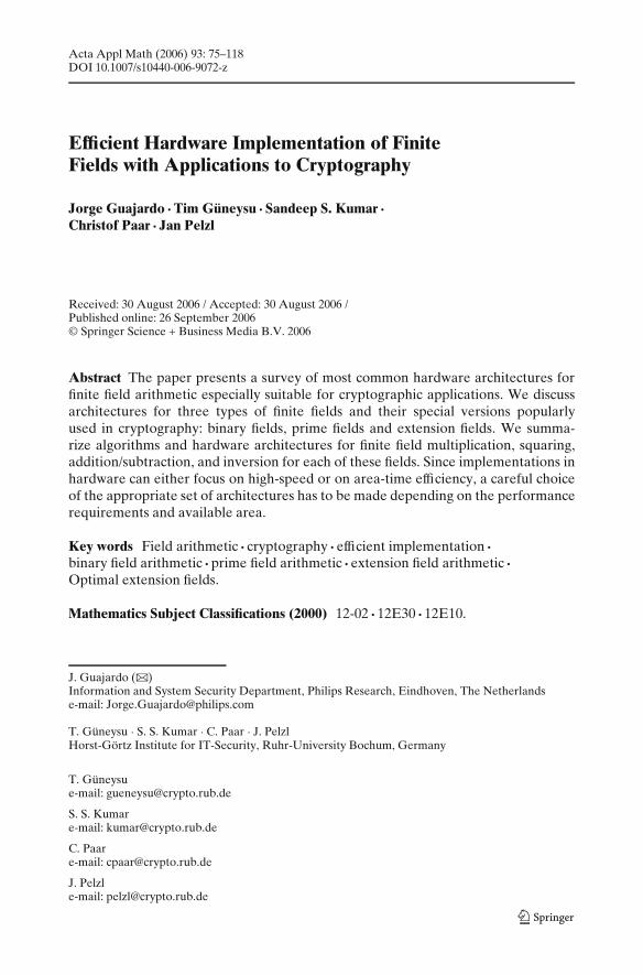
A half-adder can be seen as a single-bit binary adder that produces the 2-bit binarysum of its inputs, i.e., a+ b = (cout s)2. In a similar manner, a full-adder accepts a3-bit input a, b and a carry-in bit cin, and outputs 2 bits: a sum-bit s and a carry-outbit cout, according to Eqs. (3) and (4)

s = a⊕ b ⊕ cin (3)

cout = (a ∧ b ) ∨ (cin ∧ (a∨ b ))

= (a ∧ b ) ∨ (a ∧ cin) ∨ (b ∧ cin) (4)

Pictorially, we can view half-adders and full-adders as depicted in Figures 1 and 2.In the next paragraph, we will discuss the simplest version of an adder and how

adders can be used for subtraction.

2.1.2 Ripple-Carry Adders (RCA)

An n-bit ripple-carry adder (RCA) can be synthesized by concatenating n single-bitFA cells, with the carry-out bit of the ith-cell used as the carry-in bit of the (i+ 1)th-cell. The resulting n-bit adder outputs an n-bit long sum and a carry-out bit.

Addition and subtraction usually is implemented as a single circuit. A subtractionx− y can simply be computed by the addition of x, y, and 1, where y is the bitwisecomplement of y. Hence, the subtraction can rely on the hardware for addition.

Figure 1 Half-adder cell.

cout

HA

s

a b

Acta Appl Math (2006) 93: 75–118 79

Figure 2 Full-adder cell.

cout

cin

FA

s

a b

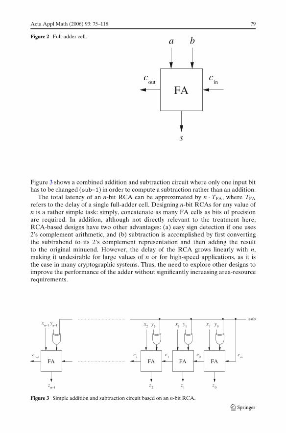
Figure 3 shows a combined addition and subtraction circuit where only one input bithas to be changed (sub=1) in order to compute a subtraction rather than an addition.

The total latency of an n-bit RCA can be approximated by n · TFA, where TFA

refers to the delay of a single full-adder cell. Designing n-bit RCAs for any value ofn is a rather simple task: simply, concatenate as many FA cells as bits of precisionare required. In addition, although not directly relevant to the treatment here,RCA-based designs have two other advantages: (a) easy sign detection if one uses2’s complement arithmetic, and (b) subtraction is accomplished by first convertingthe subtrahend to its 2’s complement representation and then adding the resultto the original minuend. However, the delay of the RCA grows linearly with n,making it undesirable for large values of n or for high-speed applications, as it isthe case in many cryptographic systems. Thus, the need to explore other designs toimprove the performance of the adder without significantly increasing area-resourcerequirements.

Figure 3 Simple addition and subtraction circuit based on an n-bit RCA.

80 Acta Appl Math (2006) 93: 75–118

2.1.3 Carry-Lookahead Adders (CLA)

As its name indicates a carry lookahead adder (CLA) computes the carries generatedduring an addition before the addition process takes place, thus, reducing the totaltime delay of the RCA at the cost of additional logic. In order to compute carriesahead of time we define next generate, propagate, and annihilate signals.

Definition 1 Let ai, b i be two operand digits in radix-r notation and ci be the carry-in digit. Then, we define the generate signal gi, the propagate signal pi, and theannihilate (absorb) signal vi as:

gi = 1 if ai + bi ≥ r

pi = 1 if ai + bi = r − 1

vi = 1 if ai + bi < r − 1

where ci, gi, pi, vi ∈ {0, 1} and 0 ≤ ai, bi < r.

Notice that Definition 1 is independent of the radix used which allows one to treatthe carry propagation problem independently of the number system [55]. Specializingto the binary case and using the signals from Definition 1, we can re-write gi, pi, andvi as:

gi = ai ∧ bi (5)

pi = ai ⊕ bi (6)

vi = ai ∧ bi = ai ∨ bi (7)

Relations (5), (6), and (7) have very simple interpretations. If ai, bi ∈ GF(2), thena carry will be generated whenever both ai and bi are equal to 1, a carry will bepropagated if either ai or bi are equal to 1, and a carry will be absorbed wheneverboth input bits are equal to 0. In some cases it is also useful to define a transfer signal(ti = ai ∨ bi) which denotes the event that the carry-out will be 1 given that the carry-in is equal to 1.2 Combining Eqs. (4), (5), and (6) we can write the carry-recurrencerelation as follows:

ci+1 = gi ∨ (ci ∧ ti) = gi ∨ (ci ∧ pi) (8)

Intuitively, Eq. (8) says that there will be a non-zero carry at stage i+ 1 either ifthe generate signal is equal to 1 or there was a carry at stage i and it was propagated(or transferred) by this stage. Notice that implementing the carry-recurrence usingthe transfer signal leads to slightly faster adders than using the propagate signal, since

2 Notice that different authors use different definitions. We have followed the definitions of [55],however [42] only defines two types of signals a generate signal, which is the same as the generatesignal from [55], and a propagate signal which is equivalent to [55] transfer signal. The resulting carryrecurrence relations are nevertheless the same.

Acta Appl Math (2006) 93: 75–118 81

an OR gate is easier to produce than an XOR gate [55]. Notice that from Eqs. (3)and (6), it follows that

si = pi ⊕ ci (9)

Thus, Eqs. (9) and (8) define the CLA.

2.1.4 Carry-Save Adders (CSA)

A CSA is simply a parallel ensemble of n full-adders without any horizontalconnection, i.e., the carry bit from adder i is not fed to adder i+ 1 but rather,stored as c′i. In particular given three n-bit integers A =∑n−1

i=0 ai2i, B =∑n−1i=0 bi2i,

and C =∑n−1i=0 ci2i, their sum produces two integers C′ =∑n

i=0 c′i2i and S =∑n−1

i=0 si2i

such that

C′ + S = A+ B+ C

where:

si = ai ⊕ bi ⊕ ci (10)

c′i+1 = (ai ∧ bi) ∨ (ai ∧ ci) ∨ (bi ∧ ci) (11)

where c′0 = 0 (notice that Eqs. (10) and (11) are nothing else but Eqs. (1) and (2)re-written for different inputs and outputs). An n-bit CSA is shown in Figure 4.

We point out that since the inputs A, B, and C are all applied in parallel the totaldelay of a CSA is equal to that of a full-adder cell (i.e., the delay of Eqs. (10) and(11)). On the other hand, the area of the CSA is just n-times the area of an FAcell and it scales very easily by adding more FA-cells in parallel. Subtraction can beaccomplished by using 2’s complement representation of the inputs.

However, CSAs have two major drawbacks:

– Sign detection is hard. In other words, when an integer is represented as a carry-save pair (C′, S) such that its actual value is C′ + S, we may not know the signof the total sum C′ + S unless the addition is performed in full length. In [35] amethod for fast sign estimation is introduced and applied to the construction ofmodular multipliers.

Figure 4 n-bit carry-saveadder.

n–1an–1b

n–1c n–2c

n–2b

n–2a0a

0b0c

n–2sn–2c’n–1sn–1c’ 0s0c’

FA FA FA

82 Acta Appl Math (2006) 93: 75–118

– CSAs do not solve the problem of adding two integers and producing a singleoutput. Instead, it adds three integers and produces two outputs.

2.1.5 Carry-Delayed Adders (CDA)

Carry-delayed adders (CDAs) were originally introduced in [53] as a modificationto the CSA paradigm. In particular, a CDA is a two-level CSA. Thus, adding A =∑n−1

i=0 ai2i, B =∑n−1i=0 bi2i, and C =∑n−1

i=0 ci2i, we obtain the sum-pair (D, T), suchthat D+ T = A+ B+ C, where

si = ai ⊕ bi ⊕ ci

c′i+1 = (ai ∧ bi) ∨ (ai ∧ ci) ∨ (bi ∧ ci)

ti = si ⊕ c′i (12)

di+1 = si ∧ c′i (13)

with c′0 = d0 = 0. Notice that Eqs. (12) and (13) are exactly the same equations thatdefine a half-adder, thus an n-bit CDA is nothing else but an n-bit CSA plus a row ofn half-adders. The overall latency is equal to the delay of a full-adder and a half-addercascaded in series, whereas the total area is equal to n times the area of a full-adderand a half adder. The CDA scales in same manner as the CSA.

2.1.6 Summary and Comparison

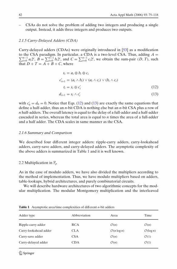
We described four different integer adders: ripple-carry adders, carry-lookaheadadders, carry-save adders, and carry-delayed adders. The asymptotic complexity ofthe above adders is summarized in Table 1 and it is well known.

2.2 Multiplication in Fp

As in the case of modulo adders, we have also divided the multipliers according tothe method of implementation. Thus, we have modulo multipliers based on adders,table-lookups, hybrid architectures, and purely combinatorial circuits.

We will describe hardware architectures of two algorithmic concepts for the mod-ular multiplication. The modular Montgomery multiplication and the interleaved

Table 1 Asymptotic area/time complexities of different n-bit adders

Adder type Abbreviation Area Time

Ripple-carry adder RCA O(n) O(n)

Carry-lookahead adder CLA O(n log n) O(log n)

Carry-save adder CSA O(n) O(1)

Carry-delayed adder CDA O(n) O(1)

Acta Appl Math (2006) 93: 75–118 83

modular multiplication allow for an area-time efficient design. Modular multiplica-tion in Fp is the mathematical operation

x · y mod p

with y, x, p ∈ Fp and x, y < p, whereby x and y are called the operands and pdenotes the modulus. In current practical cryptologic applications, x, y and p arelarge numbers of 100 bit and above. There exists many different algorithms formodular multiplication. All these algorithms belong to one of two groups:

– Parallel algorithms: most such algorithms are time optimal and calculate theresult with a time complexity of O(log p) [74]. Their disadvantage is a huge areacomplexity, resulting in an expensive hardware implementation. But many prac-tical applications require low-cost solutions, especially now where an increasingnumber of high volume products require cryptographic foundations (e.g., inconsumer electronics).

– Sequential algorithms: the sequential algorithms of highest importance are theclassical modular multiplication [36], Barrett modular multiplication [4], inter-leaved modular multiplication [11, 63], and modular Montgomery multiplica-tion [50].

In the classical modular multiplication, operands are multiplied and the resultis divided by modulus. The remainder of this division is the result of the modularmultiplication. The disadvantage of the classical modular multiplication is the size ofthe intermediate result, which is twice the size of the operands and more importantly,its area and time complexities. Barrett replaces the modular multiplication by threestandard multiplications and some additions. The disadvantage of this solutionis the high time complexity of three multiplications. During interleaved modularmultiplication the multiplication and the calculation of the remainder of the divisionare interleaved. The advantage is that the length of the intermediate result is only 1or 2 bits larger than the operands. The disadvantage is the use of subtractions in orderto reduce the intermediate results. More detailed information about interleavedmodular multiplication will be provided in the following. The modular Montgomerymultiplication is the most frequently used algorithm for modular multiplication.The computation is done in the Montgomery domain. As an advantage of thiscomputation, we do not need subtractions to reduce the intermediate results. Thedisadvantage is the fact that the modular Montgomery multiplication calculates

x · y · 2−k (mod p) instead of x · y (mod p).

Hence, two modular Montgomery multiplications are required for one modular mul-tiplication. More detailed information about modular Montgomery multiplication isgiven in following paragraphs.

2.2.1 Interleaved Modular Multiplication

The idea of interleaved modular multiplication is quite simple: the first operandis multiplied with the second operand in a bitwise manner and added to theintermediate result. The intermediate result is reduced with respect to the modulus.

84 Acta Appl Math (2006) 93: 75–118

Algorithm 1 Interleaved Modular MultiplicationInput: x, y, p with 0 ≤ x, y ≤ pOutput: u = x · y mod p

k: number of bits of xxi: ith bit of x

1: u = 0;2: for i = k− 1; i ≥ 0; i = i− 1 do3: u = 2 · u;4: v = xi · y;5: u = u+ v;6: if u ≥ p then7: u = u− p;8: end if9: if u ≥ p then

10: u = u− p;11: end if12: end for

For this purpose two subtractions per iteration are required. Algorithm 1 providesa pseudo code description of interleaved modular multiplication. Algorithm 1 hasseveral drawbacks: the first problem is the comparison of u and p in Steps 6 and 9. Inthe worst case all bits of p and u must be compared. This problem can be solved byan approximate comparison with 2k instead of p. The second problem is the numberof additions or subtractions in Steps 5, 7, and 10. All these operations can be replacedby one addition only. In order to do so, we estimate the number of times p should besubtracted, and find out if y will be added in the next loop iteration. There are onlyfew possible values for this estimation. These can be precomputed and stored in alook-up table. In each loop iteration, the estimation of the previous iteration can beadded to the intermediate result. Figure 5 depicts an optimized architecture of theinterleaved modular multiplication.

The advantage of this version is the fact that only one addition per iteration of theloop is required. It is also possible to use a CSA in order to obtain a higher clockfrequency, as suggested by [15].

2.2.2 Montgomery Modular Multiplication

Montgomery modular multiplication is based on the same concept as the interleavedmodular multiplication: the first operand is multiplied bitwise with the secondoperand. The results of these partial multiplications are added successively fromthe least significant to the most significant bit differently from interleaved modularmultiplication. In each iteration, we determine whether the intermediate result isodd or even. For this purpose the least significant bit of the intermediate result isinspected. In case this bit is equal to ‘1,’ the modulus is added to the intermediatesum. This guarantees the sum to be even. The intermediate result is then divided by2. Algorithm 2 describes the Montgomery modular multiplication.

Acta Appl Math (2006) 93: 75–118 85

Figure 5 Interleaved modular multiplication with RCA.

A modular multiplication for numbers in standard representation requires twomodular Montgomery multiplications:

z = Montgomery(x, y, p)

= x · y · 2−k mod p

and

z = Montgomery(z, 22k mod p, p)

= (x · y · 2−k mod p) · (22k mod p) · 2−k mod p

= (x · y · 2−k · 22k · 2−k) mod p

= x · y mod p.

The advantage of Algorithm 2 is that it does not require any subtractions.However, the algorithm requires two additions per loop iteration and these additionsare slow because they are non-redundant. This problem was solved an [16] where avery efficient architecture was presented for Montgomery multiplication with CSA.This architecture is shown in Figure 6.

A detailed comparison of efficient hardware architectures for Montgomery multi-plication and interleaved multiplication can be found in [3].

86 Acta Appl Math (2006) 93: 75–118

Algorithm 2 Montgomery Modular Multiplication

Input: x, y < p < 2k, with 2k−1 < p < 2k and p = 2t + 1, with t ∈ N.Output: u = x · y · 2−k mod p.

k: number of bit in x,xi: ith bit of x

1: u = 0;2: for i = 0; i < k; i++ do3: u = u+ xi · y4: if u0 = 1 then5: u = u+ p;6: end if7: u = u div 2;8: end for9: if u ≥ p then

10: u = u− p;11: end if

2.3 Architectures for Small Moduli

2.3.1 Table Look-up and Hybrid-based Architectures

The naive method to implement modular multiplication via table look-ups wouldrequire m2�log2(m) bits of storage with m = �p. Early implementations based ontable look-ups can be found in [33, 67]. However, several techniques have beendeveloped to improve on these memory requirements.

2.3.2 Combinatorial Architectures

This section considers modulo multipliers based on combinational logic for fixedmoduli. We emphasize that only architectures for fixed moduli have been considered.In addition, it would not be fair to compare architectures which can process multiplemoduli to architectures optimized for a single modulus. To our knowledge, the bestarchitectures for variable moduli in the context of RNS is the one presented in[17]. In Di Claudio et al. [17] introduced the pseudo-RNS representation. This newrepresentation is similar in flavor to the Montgomery multiplication technique as itdefines an auxiliary modulus A relatively-prime to p. The technique allows buildingreprogrammable modulo multipliers, systolization, and simplifies the computation ofDSP algorithms. Nevertheless, ROM-based solutions seem to be more efficient forsmall moduli p < 26 [17].

In Soudris et al. [66] present full-adder (FA) based architectures for RNS multiply-add operations which adopt the carry-save paradigm. The paper concludes that formoduli p > 25, FA based solutions outperform ROM ones. Finally, [57] introduces anew design which takes advantage of the non-occurring combinations of input bits toreduce certain 1-bit FAs to OR gates and, thus, reduce the overall area complexityof the multiplier. The multiplier outperforms all previous designs in terms of area.However, in terms of time complexity, the designs in [17, 61] as well as ROM-basedones outperform the multiplier proposed in [57] for most prime moduli p < 27.

Acta Appl Math (2006) 93: 75–118 87

carry save adder

register Cloop

controller

MUX MUX

shift right shift right

x i

c0 s 0

y0

register S

SC

C S

p+y (1100)(1010)(1001)

y(1110)(1101)(1011)(1000)

p(0101)(0110)(0001)(0010)

(0111)(0100)(0011)

(1111)

(0000)

MU

X

0

lsb lsb

Figure 6 Montgomery modular multiplication with one CSA.

88 Acta Appl Math (2006) 93: 75–118

Nevertheless, the combined time/area product in [57] is always less than that ofother designs.

2.4 Inversion in Fp

Several cryptographic methods based on prime fields Fp require an operation toabsorb the effect of a modular multiplication and hence find for a given value a, anumber b = a−1 mod p which fulfills the congruence a · b ≡ 1 mod p. To find sucha corresponding number b , we basically have two directions for an implementation.The first is based on exploiting Fermat’s little theorem which translates into modularexponentiation and the second relies on the principle of the extended Euclidean(GCD) algorithm. Unfortunately, both approaches have significant disadvantages,hence a lot of efforts have been taken to avoid or combine modular inversionsas often as possible by algorithmic modifications. In Elliptic Curve Cryptographyfor example, the projective point representation is usually preferred for hardwareapplication because it trades inversions for multiplications which simplifies a designenormously in terms of area costs.

2.4.1 Fermat’s Little Theorem

From Fermat’s little theorem we know that ap−1 ≡ 1 mod p. With this theorem, themodular inversion can be easily implemented by computing b = a−1 ≡ ap−2 mod p.This obviously can be implemented in hardware by an exponentiation fundamentallyrelying on a clever choice of an underlying modular multiplication method (c.f.Section 2.2) which is repetitively applied. The original multiplication hardware isaugmented by an exponentiation controller either implementing a classical binarymethod or using a more advanced windowing technique. The smarter methods,however, usually require additional precomputations and, thus, additional memoryto store the precomputed values. Figure 7 shows the basic schematic of a simpleFermat based binary exponentiation circuit.

Figure 7 Finite field inversionover Fp using exponentiationhardware.

modularmultiplication

shift register p-2

loopcontroller

register mi

a

a-1

MUX

mi-1

(p-2)i

Acta Appl Math (2006) 93: 75–118 89

The drawback of this type of approach is the slow execution speed for a singleinversion. In particular, exponentiation has an overall complexity of O(n3). Ahardware implementation which employs the Fermat based method has an areacomplexity of O(n2) and a time complexity of O(n2), respectively. This is oftenunacceptable. Hence, further attempts to reduce the execution time of an inversionwill be shown in the next section.

2.4.2 Extended GCD Algorithms

Another approach to inversion is the implementation of the extended Euclideanalgorithm (EEA) which computes the modular inverse of a number a ∈ Fp by findingtwo variables b , q that satisfy the relation

ab + pq = gcd(a, p) = 1

Computing mod p on both sides of the equation, the term pq vanishes and the inverseof a is finally obtained as b . The operation of the EEA is based on the iterativecomputation of the gcd(a, m) with corresponding updates of the intermediate com-binations of the coefficients leading to b , q. Due to the costly divisions in hardwarewhich are required to compute the GCD, binary variants have been developed whichare more appropriate for an implementation in hardware. Additionally, the Kaliskialgorithm which is based on a two step computation of such a binary EEA variantis capable to perform an inversion between standard integer and Montgomerydomain [49].

2.4.3 Binary Extended Euclidean Algorithm (BEA)

The Binary Extended Euclidean Algorithm was first proposed by R. Silver andJ. Tersian in 1962 and it was published by G. Stein in 1967 [37]. It trades the divisionsperformed in the original EEA method for bit shifts which are much better suited forhardware applications. Hence, the algorithm can be efficiently implemented usingjust adder and subtracter circuits in combination with shift registers for the division.This benefit in the reduction of hardware complexity is at the expense of an increasednumber of iterations. Here, the upper bound for the iteration count turns out tobe 2(

⌊log2 x

⌋+ ⌊log2 y⌋+ 2) [51]. Although several authors have proposed efficient

hardware architectures and implementations for the BEA [69, 71], more recentresearch has concentrated on the development of Montgomery based inversionwhich will be discussed in greater detail in the next section. Modular arithmetic inthe Montgomery domain over Fp always has the great advantage of a straightforwardmodular reduction instead of a costly division.

2.4.4 Kaliski Inversion for Montgomery Domain

The modular inverse for Montgomery arithmetic was first introduced by Kaliski in1995 [34] as a modification of the extended binary GCD algorithm. This methodprovides some degree of computational freedom by finding the modular inverse intwo phases: First, for a given value a ∈ Fp in standard representation or a · 2m ∈ Fp

in the Montgomery domain, an almost modular inverse r with r = a−1 · 2z mod p iscomputed. Secondly, the output r is corrected by a second phase which reduces the

90 Acta Appl Math (2006) 93: 75–118

Table 2 Configurations of the Kaliski inversion for different domains

Domain After phase I Phase II operation Total complexity

Standard→ Standard r = a−1 · 2z r = (r + p · r0)/2 2z

Standard→Montgomery r = a−1 · 2z r = (r + p · r0)/2 2z −m

Montgomery→ Standard r = a−1 · 2z−h r = 2(r − p · r0) 2z −m

Montgomery→Montgomery r = a−1 · 2z−h r = 2(r − p · r0) 2m

exponent z in r either to z = 0 or z = m of the target domain. Thus, the algorithm canbe used for several combinations for converting values from and to the Montgomerydomain. Table 2 shows the possible options and their corresponding necessaryiteration count and the required type of operation for the correction performed inthe second phase. Note that due to the n-bit modulus p with p > a, the exponent zis always in the range n < z < 2n. Hence, in the worst case 4n− 2 iterations have tobe performed for determining the modular inverse in standard domain whereas theinverse in Montgomery representation solely requires about 2m where m denotes theMontgomery radix.

From the sequential structure of Algorithm 3 it becomes clear that a direct transferto a hardware architecture suffers from a long critical path due to inner conditions aswell as the necessity for several parallel arithmetic components. Thus, the inversionis costly in terms of area with a relatively low maximum clocking speed compared

Algorithm 3 Almost Montgomery Inverse (AMI)Input: a ∈ Fp

Output: r and z where r = a−1 · 2z mod p and m ≤ z ≤ 2m1: u← p, v← a, r← 0, s← 12: k← 03: while v > 0 do4: if u is even then5: u← u/2, s← 2s6: else if v is even then7: v← v/2, r← 2r8: else if u > v then9: u← (u− v)/2, r← r + s, s← 2s

10: else11: v← (v − u)/2, s← r + s, r← 2r12: end if13: k← k+ 114: end while15: if r ≥ p then16: r← r − p {Make sure that r is within its boundaries}17: end if18: return r← p− r

Acta Appl Math (2006) 93: 75–118 91

Figure 8 Basic Kaliski inversion design.

to the proposed architectures for multiplication and addition in previous sections. Abasic inverter design is shown in Figure 8 based on one n-bit adder and two n-bitsubtracters.

There are several improvements to minimize hardware requirements and signallatency of the Kaliski inverter due to the long carry propagation path in the n-bit wideadders and subtracters. An efficient VLSI architecture has been described in [29],whereas in [22] the total critical path is reduced by using n/2-bit arithmetics whichenables a higher clocking frequency and increases the overall throughput. An areaoptimized inversion design, however, was reported in [10] by Bucik and Lorencz.The authors modified the AMI algorithm by introducing 2’s-complement numberrepresentation which relaxed the critical path dependencies and allowed for a designusing only a single n-bit adder and subtracter.

3 Extension Fields F2m and Fpm : Preliminaries

3.1 Basis Representation

For the discussion that follows, it is important to point out that there are severalpossibilities to represent elements of extension fields. Thus, in general, given an irre-ducible polynomial F(x) of degree m over Fq and a root α of F(x) (i.e., F(α) = 0), onecan represent an element A ∈ Fqm , q = pn and p prime, as a polynomial in α, i.e., asA = am−1α

m−1 + am−2αm−2 + · · · + a1α + a0 with ai ∈ Fq. The set {1, α, α2, . . . , αm−1}

is then said to be a polynomial basis (or standard basis) for the finite field Fqm overFq. Another type of basis is called a normal basis. Normal bases are of the form{β, βq, βq2

, . . . , βqm−1} for an appropriate element β ∈ Fqm . Then, an element B ∈ Fqm

can be represented as B = bm−1βqm−1 + bm−2β

qm−2 + · · · + b1βq + b0β where bi ∈ Fq.

It can be shown that for any field Fq and any extension field Fqm , there exists alwaysa normal basis of Fqm over Fq(see [43, Theorem 2.35]). Notice that (βqi

)qk = βqi+k =

92 Acta Appl Math (2006) 93: 75–118

βqi+k mod mwhich follows from the fact that βqm ≡ β (i.e., Fermat’s little theorem). Thus,

raising an element B ∈ Fqm to the qth power can be easily accomplished througha cyclic shift of its coordinates, i.e., Bq = (bm−1β

qm−1 + bm−2βqm−2 + · · · + b1β

q +b0β)q = bm−2β

qm−1 + bm−3βqm−2 + · · · + b0β

q + bm−1β , where we have used the factthat in any field of characteristic p, (x+ y)q = xq + yq, where q = pn. Finally, thedual basis has also received attention in the literature. Two bases {α0, α1, . . . , αm−1}and {β0, β1, . . . , βm−1} of Fqm over Fq are said to be dual or complementary bases iffor 0 ≤ i, j ≤ m− 1 we have:

TrE/F (αiβj) =⎧⎨

⎩

0 for i = j

1 for i = j

A variation on dual bases is introduced in [48, 75] where the concept of a weakly dualbasis is defined. As a final remark notice that given a basis {α0, α1, . . . , αm−1} of Fqm

over Fq, one can always represent an element β ∈ Fqm as:

β = b0α0 + b1α1 + · · · + bm−1αm−1

where bi ∈ Fq.

3.2 Notation

In Sections 4 and 5 we describe hardware implementation techniques for fields F2m

and Fpm , where p is odd, respectively. Thus, in general we can speak of the fieldFpm , where p = 2 in the case of F2m and odd otherwise. The field is generated byan irreducible polynomial F(x) = xm + G(x) = xm +∑m−1

i=0 gixi over Fp of degree m.We assume α to be a root of F(x), thus for A, B, C ∈ Fpm , we write A =∑m−1

i=0 aiαi,

B =∑m−1i=0 biα

i, C =∑m−1i=0 ciα

i, and ai, bi, ci ∈ Fp. Notice that by assumption F(α) =0 since α is a root of F(x). Therefore,

αm = −G(α) =m−1∑

i=0

−giαi (14)

gives an easy way to perform modulo reduction whenever we encounter powers of α

greater than m− 1. Eq. (14) reduces to

αm = G(α) =m−1∑

i=0

giαi (15)

for fields of characteristic 2. Addition in Fpm can be achieved as shown in Eq. (16)

C(α) ≡ A(α)+ B(α) =m−1∑

i=0

(ai + bi)αi (16)

where the addition ai + bi is done in Fp, (e.g. ai ∈ {0, 1} for F2m ). Multiplication oftwo elements A, B ∈ Fpm is written as C(α) =∑m−1

i=0 ciαi ≡ A(α) · B(α), where the

multiplication is understood to happen in the finite field Fpm and all αt, with t ≥ mcan be reduced using Eq. (14). Notice that we abuse our notation and throughoutthe text we will write A mod F(α) to mean explicitly the reduction step describedpreviously. Finally, we refer to A as the multiplicand and to B as the multiplier.

Acta Appl Math (2006) 93: 75–118 93

4 Hardware Implementation Techniques for Fields F2m

Characteristic 2 fields F2m are often chosen for hardware realizations [12] as they arewell suited for hardware implementation due to their ‘carry-free’ arithmetic. Thisnot only simplifies the architecture but reduces the area due to the lack of carryarithmetic. For hardware implementations trinomial and pentanomial reductionpolynomials are chosen as they enable a very efficient implementation. We presenthere efficient architectures for multiplier and squarer implementations for binaryfields in hardware. The inversion architecture is similar in design to that used inthe extension fields of odd characteristic described in Section 6 and is therefore notdiscussed here.

4.1 Multiplication in F2m

Multiplication of two elements A, B ∈ F2m , with A(α) =∑m−1i=0 aiα

i and B(α) =∑m−1

i=0 biαi is given as

C(α) =m−1∑

i=0

ciαi ≡ A(α) · B(α) mod F(α)

where the multiplication is a polynomial multiplication, and all αt, with t ≥ m arereduced with Eq. (15). The simplest algorithm for field multiplication is the shift-and-add method [37] with the reduction step inter-leaved shown as Algorithm 4.

Notice that in Step 3 of Algorithm 4 the computation of bi A and Cα mod F(α) canbe performed in parallel as they are independent of each other. However, the valueof C in each iteration depends on both the value of C at the previous iteration andon the value of bi A. This dependency has the effect of making the MSB multiplierhave a longer critical path than that of the Least Significant Bit (LSB) multiplier,described later in the next section.

For hardware, the shift-and-add method can be implemented efficiently and issuitable when area is constrained. When the bits of B are processed from the most-significant bit to the least-significant bit (as in Algorithm 4), then it receives the nameof Most-Significant Bit-serial (MSB) multiplier [65].

Algorithm 4 Shift-and-Add Most Significant Bit (MSB) First F2m Multiplication

Input: A =∑m−1i=0 aiα

i, B =∑m−1i=0 biα

i where ai, bi ∈ F2.Output: C ≡ A · B mod F(α) =∑m−1

i=0 ciαi where ci ∈ F2.

1: C← 02: for i = m− 1 downto 0 do3: C← C · α mod F(α)+ bi · A4: end for5: Return (C)

94 Acta Appl Math (2006) 93: 75–118

4.1.1 Reduction mod F(α)

In the MSB multiplier, a quantity of the form Wα, where W(α) =∑m−1i=0 wiα

i ∈ F2m ,has to be reduced mod F(α). Multiplying W by α, we obtain

Wα =m−1∑

i=0

wiαi+1 = wm−1α

m +m−2∑

i=0

wiαi+1 (17)

Using the property of the reduction polynomial as shown in Eq. (15), we cansubstitute for αm and re-write the index of the second summation in Eq. (17).Wα mod F(α) can then be calculated as follows:

Wα mod F(α) =m−1∑

i=0

(giwm−1)αi +

m−1∑

i=1

wiαi = (g0wm−1)+

m−1∑

i=1

(wi−1 + giwm−1)αi

where all coefficient arithmetic is done modulo 2. As an example, we consider thestructure of a 163-bit MSB multiplier shown in Figure 9.

Here, the operand A is enabled onto the data-bus A of the multiplier directlyfrom the memory register location. The individual bits of bi are sent from a memorylocation by implementing the memory registers as a cyclic shift-register (with theoutput at the most-significant bit).

The reduction within the multiplier is performed on the accumulating result ci, asin Step 3 in Algorithm 4. The taps that are fed back to ci are based on the reductionpolynomial. Figure 9 shows an implementation for the reduction polynomial F(x) =x163 + x7 + x6 + x3 + 1, where the taps XOR the result of c162 to c7, c6 c3 and c0. Thecomplexity of the multiplier is n AND + (n+ t − 1) XOR gates and n FF where t = 3 fora trinomial reduction polynomial and t = 5 for a pentanomial reduction polynomial.The latency for the multiplier output is n clock cycles. The maximum critical path is2�XOR (independent of n) where, �XOR represents the delay in an XOR gate.

Similarly a Least-Significant Bit-serial (LSB) multiplier can be implemented andthe choice between the two depends on the design architecture and goals. In an LSBmultiplier, the coefficients of B are processed starting from the least significant bit b0

Figure 9 F2163 Most significant bit-serial (MSB) multiplier circuit.

Acta Appl Math (2006) 93: 75–118 95

and continues with the remaining coefficients one at a time in ascending order. Thusmultiplication according to this scheme is performed in the following way:

C ≡ AB mod F(α)

≡ b0 A+ b1(Aα mod F(α))+ b2(Aα2 mod F(α))

+ . . .+ bm−1(Aαm−1 mod F(α))

≡ b0 A+ b1(Aα mod F(α))+ b2((Aα)α mod F(α))

+ . . .+ bm−1((Aαm−2)α mod F(α))

4.1.2 Digit Multipliers

Introduced by Song and Parhi in [65], they consider trade-offs between speed, area,and power consumption. This is achieved by processing several of B’s coefficients atthe same time. The number of coefficients that are processed in parallel is defined tobe the digit-size D. The total number of digits in the polynomial of degree m− 1 isgiven by d = �m/D. Then, we can re-write the multiplier as B =∑d−1

i=0 BiαDi, where

Bi =D−1∑

j=0

bDi+ jαj , 0 ≤ i ≤ d− 1 (18)

and we assume that B has been padded with zero coefficients such that bi = 0for m− 1 < i < d · D (i.e., the size of B is d · D coefficients but deg(B) < m). Themultiplication can then be performed as:

C ≡ A · B mod F(α) = Ad−1∑

i=0

BiαDi mod F(α) (19)

The Least-Significant Digit-serial (LSD) multiplier is a generalization of the LSBmultiplier in which the digits of B are processed starting from the least significant tothe most significant. Using Eq. (19), the product in this scheme can be computed asfollows

C ≡ A · B mod F(α)

≡ [B0 A+ B1(

AαD mod F(α))+ B2

(AαDαD mod F(α)

)

+ . . .+ Bd−1(

AαD(d−2)αD mod F(α))]

mod F(α)

Algorithm 5 shows the details of the LSD Multiplier.

Remark 1 If C is initialized to value I ∈ F2m in Algorithm 5, then we can obtain asoutput the quantity, A · B+ I mod F(α) at no additional (hardware or delay) cost.This operation, known as a multiply/accumulate operation is very useful in ellipticcurve based systems.

96 Acta Appl Math (2006) 93: 75–118

Algorithm 5 Least Significant Digit-serial (LSD) Multiplier [65]


i, where ai ∈ F2, B =∑� mD −1

i=0 BiαDi, where Bi as in Eq. (18)

Output: : C ≡ A · B =∑m−1i=0 ciα

i, where ci ∈ F2

1: C← 02: for i = 0 to �m

D − 1 do3: C← Bi A+ C4: A← AαD mod F(α)

5: end for6: Return (C mod F(α))

4.1.3 Reduction mod F(α) for Digit Multipliers

In an LSD multiplier, products of the form WαD mod F(α) occur (as seen in Step 4 ofAlgorithm 5) which have to be reduced. As in the LSB multiplier case, one can deriveequations for the modular reduction for general irreducible F(α) polynomials. How-ever, it is more interesting to search for polynomials that minimize the complexity ofthe reduction operation. In coming up with these optimum irreducible polynomialswe use two theorems from [65].

Theorem 1 [65] Assume that the irreducible polynomial is of the form F(α) = αm +gkα

k +∑k−1j=0 g jα

j, with k < m. For t ≤ m− 1− k, αm+t can be reduced to degree lessthan m in one step with the following equation:

αm+t mod F(α) = gkαk+t +

k−1∑

j=0

g jαj+t (20)

Theorem 2 [65] For digit multipliers with digit-element size D, when D ≤ m− k, theintermediate results in Algorithm 5 (Step 4 and Step 6) can be reduced to degree lessthan m in one step.

Theorems 1 and 2, implicitly say that for a given irreducible polynomial F(α) =αm + gkα

k +∑k−1j=0 g jα

j, the digit-element size D has to be chosen based on the valueof k, the second highest degree in the irreducible polynomial.

The architecture of the LSD multiplier is shown in Figure 10 and consists of threemain components.

1. The main reduction circuit to shift A left by D and reduce the result modF(α)

(Step 4 Algorithm 5).2. The multiplier core which computes the intermediate C and stores it in the

accumulator (Step 3 Algorithm 5).3. The final reduction circuit to reduce the contents in the accumulator to get the

final result C (Step 6 Algorithm 5).

All the components run in parallel requiring one clock cycle to complete each stepand the critical path of the whole multiplier normally depends on the critical path ofthe multiplier core.

Acta Appl Math (2006) 93: 75–118 97

Figure 10 LSD-single accumulator multiplier architecture.

Figure 11 SAM core.

Acc

m+D-1

A.bDi+0

A.bDi+1

A.bDi+2

A.bDi+3

A.bDi+4

98 Acta Appl Math (2006) 93: 75–118

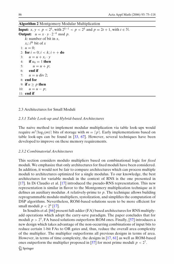
Figure 12 SAM mainreduction circuit.

Dm

D

k+1

AαDD

We provide here an analysis of the area requirements and the critical path of thedifferent components of the multiplier. In what follows, we will refer to multiplierswith a single accumulator as Single-Accumulator-Multipliers or SAM for short. InFigures 11, 12, and 13, we denote an AND gate with a filled dot and elements tobe XORed by a shaded line over them. The number of XOR gates and the criticalpath is based on the assumption that a binary tree structure is used to XOR therequired elements. For n elements, the number of XOR gates required is n− 1and the critical path delay becomes the binary tree depth �log2 n. We calculate thecritical path as a function of the delay of one XOR gate( �XOR) and one AND gate(�AND). This allows our analysis to be independent of the cell-technology used forthe implementation.

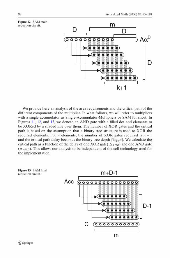
Figure 13 SAM finalreduction circuit. m+D-1

D-1

m

Acc

C

Acta Appl Math (2006) 93: 75–118 99

4.1.4 SAM Core

The multiplier core performs the operation C← Bi A+ C (Step 4 Algorithm 5).The implementation of the multiplier core is as shown in Figure 11 for a digit sizeD = 4. It consists of ANDing the multiplicand A with each element of the digit ofthe multiplier B and XORing the result into the accumulator Acc. The multipliercore requires mD AND gates (denoted by the black dots), mD XOR gates (forXORing the columns denoted by the shaded line) and m+ D− 1 Flip-Flops (FF)for accumulating the result C.

It can be seen that the multiplier core has a maximum critical path delay of one�AND (since all the ANDings in one column are done in parallel) and the delay forXORing D+ 1 elements as shown in Figure 11. Thus the total critical path delay ofthe multiplier core is �AND + �log2(D+ 1)�XOR.

4.1.5 SAM Main Reduction Circuit

The main reduction circuit performs the operation A← AαD mod F(α) (Step 3Algorithm 5) and is implemented as in Figure 12. Here the multiplicand A is shiftedleft by the digit-size D which is equivalent to multiplying by αD. The result is thenreduced with the reduction polynomial by ANDing the higher D elements of theshifted multiplicand with the reduction polynomial F(α) (shown in the figure aspointed arrows) and XORing the result. We assume that the reduction polynomial ischosen according to Theorem 2 which allows reduction to be done in one single step.We can then show that the critical path delay of the reduction circuit is equal to orless than that of the multiplier core.

The main reduction circuit requires (k+ 1) ANDs and k XORs gates for eachreduction element. The number of XOR gates is one less because the last element ofthe reduction are XORed to empty elements in the shifted A. Therefore a total of(k+ 1)D AND and kD XOR are needed for D digits. Further m FF are needed tostore A and k+ 1 FFs to store the general reduction polynomial.

The critical path of the main reduction circuit (as shown in Figure 12) is one AND(since the ANDings occur in parallel) and the critical path for summation of the Dreduction components with the original shifted A. Thus the maximum critical pathdelay is �AND + �log2(D+ 1)�XOR, which is the same as the critical path delay ofthe multiplier core.

4.1.6 SAM Final Reduction Circuit

The final reduction circuit performs the operation C mod F(α), where C of sizem+ D− 2. It is implemented as shown in Figure 13 which is similar to the mainreduction circuit without any shifting. Here the most significant (D− 1) elementsare reduced using the reduction polynomial F(α) similarly shown with arrows. Thearea requirement for this circuit is (k+ 1)(D− 1) AND gates and (k+ 1)(D− 1)

XOR gates. The critical path of the final reduction circuit is �AND + �log2(D)�XOR

which is less than that of the main reduction circuit since the size of the polynomialreduced is one smaller (Figure 13).

An r-nomial reduction polynomial satisfying Theorem 2, i.e.∑k

i=0 gi = (r − 1), isa special case and hence the critical path is upper-bounded by that obtained for

100 Acta Appl Math (2006) 93: 75–118

the general case. For a fixed r-nomial reduction polynomial, the area for the mainreduction circuit is (r − 1)D ANDs, (r − 2)D XORs and m FFs. No flip flops arerequired to store the reduction polynomial as it can be hardwired.

4.2 Squaring in F2m

Polynomial basis squaring of C ∈ F2m is implemented by expanding C to double itsbit-length by interleaving 0 bits in between the original bits of C and then reducingthe double length result as shown here:

C ≡ A2 mod F(α)

≡ (am−1α2(m−1) + am−2α

2(m−2) + . . .+ a1α2 + a0) mod F(α)

In hardware, these two steps can be combined if the reduction polynomial has asmall number of non-zero coefficients such as in the case of irreducible trinomialsand pentanomials. The architecture of the squarer implemented as a hardwiredXOR circuit is shown in Figure 14. Here, the squaring is efficiently implementedfor F(x) = x163 + x7 + x6 + x3 + 1, to generate the result in one single clock cyclewithout huge area requirements. It involves first the expansion by interleaving with0s, which in hardware is just an interleaving of 0 bit valued lines on to the bus toexpand it to 2n bits. The reduction of this polynomial is inexpensive, first, due to thefact that reduction polynomial used is a pentanomial, and secondly, the polynomialbeing reduced is sparse with no reduction required for �n/2� of the higher order bits(since they have been set to 0s).

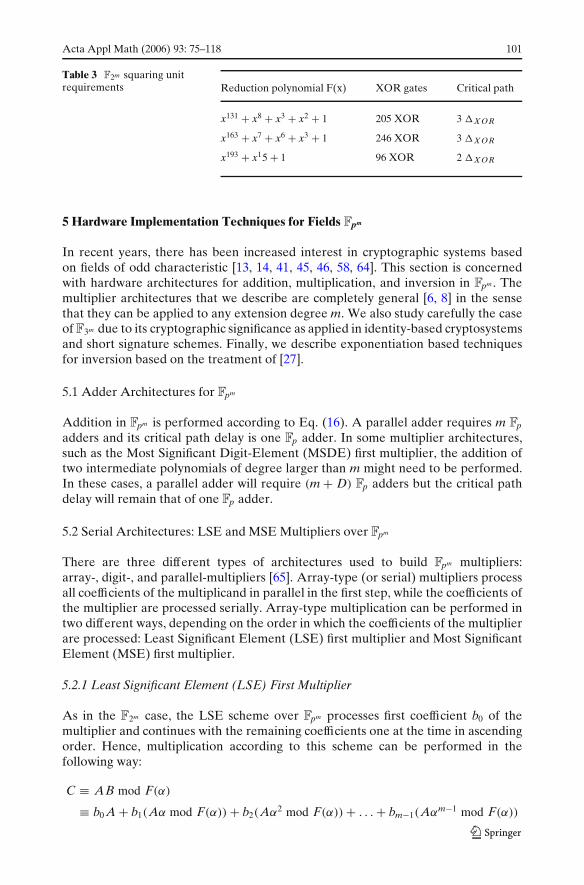
The XOR requirements and the maximum critical path (assuming an XOR treeimplementation) for three different reduction polynomials used in elliptic curvecryptography are given in Table 3.

Figure 14 F2163 squaring circuit.

Acta Appl Math (2006) 93: 75–118 101

Table 3 F2m squaring unitrequirements Reduction polynomial F(x) XOR gates Critical path

x131 + x8 + x3 + x2 + 1 205 XOR 3 �X OR

x163 + x7 + x6 + x3 + 1 246 XOR 3 �X OR

x193 + x15 + 1 96 XOR 2 �X OR

5 Hardware Implementation Techniques for Fields Fpm

In recent years, there has been increased interest in cryptographic systems basedon fields of odd characteristic [13, 14, 41, 45, 46, 58, 64]. This section is concernedwith hardware architectures for addition, multiplication, and inversion in Fpm . Themultiplier architectures that we describe are completely general [6, 8] in the sensethat they can be applied to any extension degree m. We also study carefully the caseof F3m due to its cryptographic significance as applied in identity-based cryptosystemsand short signature schemes. Finally, we describe exponentiation based techniquesfor inversion based on the treatment of [27].

5.1 Adder Architectures for Fpm

Addition in Fpm is performed according to Eq. (16). A parallel adder requires m Fp

adders and its critical path delay is one Fp adder. In some multiplier architectures,such as the Most Significant Digit-Element (MSDE) first multiplier, the addition oftwo intermediate polynomials of degree larger than m might need to be performed.In these cases, a parallel adder will require (m+ D) Fp adders but the critical pathdelay will remain that of one Fp adder.

5.2 Serial Architectures: LSE and MSE Multipliers over Fpm

There are three different types of architectures used to build Fpm multipliers:array-, digit-, and parallel-multipliers [65]. Array-type (or serial) multipliers processall coefficients of the multiplicand in parallel in the first step, while the coefficients ofthe multiplier are processed serially. Array-type multiplication can be performed intwo different ways, depending on the order in which the coefficients of the multiplierare processed: Least Significant Element (LSE) first multiplier and Most SignificantElement (MSE) first multiplier.

5.2.1 Least Significant Element (LSE) First Multiplier

As in the F2m case, the LSE scheme over Fpm processes first coefficient b0 of themultiplier and continues with the remaining coefficients one at the time in ascendingorder. Hence, multiplication according to this scheme can be performed in thefollowing way:

C ≡ AB mod F(α)

≡ b0 A+ b1(Aα mod F(α))+ b2(Aα2 mod F(α))+ . . .+ bm−1(Aαm−1 mod F(α))

102 Acta Appl Math (2006) 93: 75–118

Algorithm 6 LSE Multiplier


i, B =∑m−1i=0 biα

i, where ai, b i ∈ Fp

Output: C ≡ A · B =∑m−1i=0 ciα

i, where ci ∈ Fp

1: C← 02: for i = 0 to m− 1 do3: C← bi A+ C4: A← Aα mod F(α)

5: end for6: Return (C)

The accumulation of the partial product has to be performed with a polynomialadder. This multiplier computes the operation according to Algorithm 6.

5.2.2 Most Significant Element (MSE) First Multiplier

The most significant element multiplication starts with the highest coefficient of themultiplier polynomial. Hence, the multiplication can be performed in the followingway:

C ≡ AB mod F(α)

≡ (. . . (bm−1 Aα mod F(α)+ bm−2 A)α mod F(α)+ . . .+ b1 A)α mod F(α)+ b0 A

The algorithm is similar to the characteristic two case except that instead of bits weprocess elements of Fp, i.e., �log2(p) bits. Similarly whenever in the binary case weshift by one bit (multiplication by α), in the odd characteristic case, we need to shiftby �log2(p) bits.

5.2.3 Reduction mod F(α)

In both LSE and MSE multipliers a quantity Wα, where W =∑m−1i=0 wiα

i ∈ Fpm , wi ∈Fp, has to be reduced mod F(α). It can be shown that Wα mod F(α) can then becalculated as follows:

Wα mod F(α) =m−1∑

i=0

(−giwm−1)αi +

m−1∑

i=1

wiαi = (−g0wm−1)+

m−1∑

i=1

(wi−1 − giwm−1)αi

where all coefficient arithmetic is done modulo p. Once again we emphasize thatthe only differences between odd characteristic and even characteristic multipliersis that in the first case the coefficients are elements of Fp and that implies that thecoefficients are groups of �log2(p) bits. In addition, the reduction circuitry requiresadders and subtracters as opposed to only adders (XOR gates) as in the characteristictwo case.

5.3 Digit-Serial/Parallel Multipliers for Fpm

As in the characteristic 2 case, we can process more than coefficient of the multipli-cand at the time. This results in digit multipliers. The number of coefficients that are

Acta Appl Math (2006) 93: 75–118 103

processed in parallel is defined to be the digit-size and we denote it with the letterD. For a digit-size D, we can denote by d = �m/D the total number of digits ina polynomial of degree m− 1. Digit multipliers for Fpm are similar to their binarycharacteristic counterparts except that instead of groups of bits now we need toprocess groups of coefficients in parallel. As in [65], we can re-write the multiplieras B =∑d−1

i=0 BiαDi, where Bi =∑D−1

j=0 b Di+ jαj 0 ≤ i ≤ d− 1 and we assume that B

has been padded with zero coefficients such that b i = 0 for m− 1 < i < d · D (i.e. thesize of B is d · D coefficients but deg(B) < m). Hence,

C ≡ AB mod F(α) = Ad−1∑

i=0

BiαDi mod F(α)

As in the binary case, depending on the way we process the digits of the polynomialB, the multipliers can be classified as Least Significant Digit-Element first multiplier(LSDE) and Most Significant Digit-Element first multiplier (MSDE). Here, wehave introduced the word element to clarify that the digits correspond to groupsof Fp coefficients in contrast to [65] where the digits were groups of bits. Thealgorithms themselves are simple generalizations of the F2m case and so we referthe reader to Section 4 or to [6, 30] where the treatment is explicit for Fpm . Finally,notice that all ground field arithmetic is performed in Fp. Thus, Fp multipliers andadders/subtracters are required to build Fpm multipliers in contrast to the F2k case,where only AND and XOR gates are required. Subtracters (multiplication by −1)can be implemented as multiplication by p− 1. However, multiplication by αD isvery similar in both F2k and Fpm fields. The only difference is that instead of shiftingD bits (as in the F2k case), one has to shift D�log2(p) bits in Fpm fields.

5.4 Systolic and Scalable Architectures for Digit-Serial Multiplication

The work in [6] describes architectures for digital multiplication in Fpm but theirmethods have the drawback of using global signals and long wires and they requirereconfigurability to achieve their full potential. In particular, [6] uses irreducibletrinomial specific circuitry to perform modular reduction on FPGAs. Thus, thesesolutions lack flexibility in other hardware platforms such as ASICs. In this sectionwe describe the systolic architectures introduced in [8] for Fpm fields. The work in [8]has several advantages over standard digit multipliers, which include:

– By using a systolic design we use localized routing, thus avoiding the need forglobal control signals and long wires.

– Their methodology allows for ease of design and offers functional and layoutmodularity all of which are properties envisioned in good VLSI designs

– The authors in [8] modify the standard digit multiplier designs to allow forscalability as introduced in [70]. In other words, for a fixed value of the digit-size D [6, 65] and parameter d, we can perform a multiplication for any valueof m in Fpm , with fixed p, i.e., multiple irreducible polynomials are supported,making unnecessary the use of reconfigurability in FPGAs.

104 Acta Appl Math (2006) 93: 75–118

5.4.1 Systolic Least-Significant Digit Element (LSDE) First Architecture

The basic idea in [8] is to make modular reduction independent of the irreduciblemodulus F(α), by defining an alternate modulus F(α), working modulo F(α) duringthe exponentiation (scalar multiplication if considering elliptic curves) phase of thecryptographic operation and then at the end reducing modulo F(α) to obtain the finalresult. Before continuing, we illustrate the problem that [8] is trying to solve with anexample.

Example 1 Suppose you want to compute AαD mod F(α) where A∈Fpm and F(α)=αm + gkα

k +∑k−1i=0 giα

i is an optimum irreducible polynomial in the sense of [6, 65].Let A =∑d−1

i=0 AiαDi ∈ Fpm with d = �m/D, Ai a digit (i.e., a group of D Fp

coefficients). Then,

AαD ≡ αDd−1∑

i=0

AiαDi mod F(α) = Ad−1α

Dd +d−1∑

i=1

Ai−1αDi mod F(α)

AαD ≡ Ad−1αDd−m

(

−gkαk −

k−1∑

i=0

giαi

)

+d−1∑

i=1

Ai−1αDi

Notice that the first term in the reduced result depends on the value of m, in otherwords on the field size. In fact, one needs to multiply by αDd−m, which can beinstantiated as a variable shifter in hardware. This is undesirable if scalability of themultiplier is desired.

The following proposition is the basis for the architecture presented in [8].

Proposition 1 [8] Let A, B ∈ Fpm , F(α) = αm +∑m−1i=0 giα

i, be an irreducible polyno-mial over Fp, and d = �m/D. Then, A · B mod F(α) ≡ [A · B mod F(α)] mod F(α),where F(α) = αDd−m F(α).

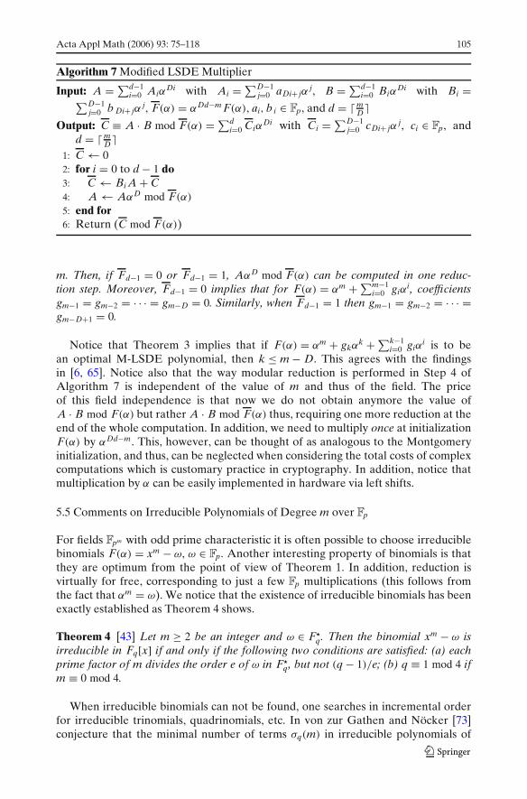
Intuitively, Proposition 1 says that we can perform reductions modulo F(α) =αDd−m F(α) and still obtain a result which when reduced modulo F(α) returns thecorrect value. Algorithm 7 shows an LSDE multiplier incorporating the modifiedmodulus of Proposition 1.

Algorithm 7 suggests the following computation strategy. Given two inputs A,

B ∈ Fpm one can compute C ≡ A · B mod F(α) by first computing C ≡ A · B modF(α) using Algorithm 7 and, then, computing C ≡ C mod F(α). The second stepfollows as a consequence of Proposition 1. In practice, the second step can beperformed at the end of a long range of computations, similar to the procedureused when performing Montgomery multiplication. Step 4 in Algorithm 7 requiresa modular multiplication. Reference [8] defines optimal polynomials which allow toreduce AαD in just one iteration and make the reduction process independent of thevalue of m and, thus, of the field Fpm .

Theorem 3 [8] Let A =∑d−1i=0 Aiα

Di be as defined in Algorithm 7 and F(α) =αDd−m F(α) = αDd +∑d−1

i=0 FiαDi be such that F(α) is irreducible over Fp of degree

Acta Appl Math (2006) 93: 75–118 105

Algorithm 7 Modified LSDE Multiplier

Input: A =∑d−1i=0 Aiα

Di with Ai =∑D−1j=0 aDi+ jα

j, B =∑d−1i=0 Biα

Di with Bi =∑D−1

j=0 b Di+ jαj, F(α) = αDd−m F(α), ai, b i ∈ Fp, and d = �m

DOutput: C ≡ A · B mod F(α) =∑d

i=0 CiαDi with Ci =∑D−1

j=0 cDi+ jαj, ci ∈ Fp, and

d = �mD

1: C← 02: for i = 0 to d− 1 do3: C← Bi A+ C4: A← AαD mod F(α)

5: end for6: Return (C mod F(α))

m. Then, if Fd−1 = 0 or Fd−1 = 1, AαD mod F(α) can be computed in one reduc-tion step. Moreover, Fd−1 = 0 implies that for F(α) = αm +∑m−1

i=0 giαi, coefficients

gm−1 = gm−2 = · · · = gm−D = 0. Similarly, when Fd−1 = 1 then gm−1 = gm−2 = · · · =gm−D+1 = 0.

Notice that Theorem 3 implies that if F(α) = αm + gkαk +∑k−1

i=0 giαi is to be

an optimal M-LSDE polynomial, then k ≤ m− D. This agrees with the findingsin [6, 65]. Notice also that the way modular reduction is performed in Step 4 ofAlgorithm 7 is independent of the value of m and thus of the field. The priceof this field independence is that now we do not obtain anymore the value ofA · B mod F(α) but rather A · B mod F(α) thus, requiring one more reduction at theend of the whole computation. In addition, we need to multiply once at initializationF(α) by αDd−m. This, however, can be thought of as analogous to the Montgomeryinitialization, and thus, can be neglected when considering the total costs of complexcomputations which is customary practice in cryptography. In addition, notice thatmultiplication by α can be easily implemented in hardware via left shifts.

5.5 Comments on Irreducible Polynomials of Degree m over Fp

For fields Fpm with odd prime characteristic it is often possible to choose irreduciblebinomials F(α) = xm − ω, ω ∈ Fp. Another interesting property of binomials is thatthey are optimum from the point of view of Theorem 1. In addition, reduction isvirtually for free, corresponding to just a few Fp multiplications (this follows fromthe fact that αm = ω). We notice that the existence of irreducible binomials has beenexactly established as Theorem 4 shows.

Theorem 4 [43] Let m ≥ 2 be an integer and ω ∈ F�q. Then the binomial xm − ω is

irreducible in Fq[x] if and only if the following two conditions are satisfied: (a) eachprime factor of m divides the order e of ω in F�

q, but not (q− 1)/e; (b) q ≡ 1 mod 4 ifm ≡ 0 mod 4.

When irreducible binomials can not be found, one searches in incremental orderfor irreducible trinomials, quadrinomials, etc. In von zur Gathen and Nöcker [73]conjecture that the minimal number of terms σq(m) in irreducible polynomials of

106 Acta Appl Math (2006) 93: 75–118

degree m over Fq, q a power of a prime, is for m ≥ 1, σ2(m) ≤ 5 and σq(m) ≤ 4 forq ≥ 3. This conjecture has been verified for q = 2 and m ≤ 10, 000 [7, 25, 73, 78–80]and for q = 3 and m ≤ 539 [72].

By choosing irreducible polynomials with the least number of non-zero coeffi-cients, one can reduce the area complexity of the LSDE multiplier. Reference [30]notices that by choosing irreducible polynomials such that their non-zero coefficientsare all equal to p− 1 one can further reduce the complexity of the multiplier. Noticethat there is no existence criteria for irreducibility of trinomials over any field Fpm .The most recent advances in this area are the results of Loidreau [44], where atable that characterizes the parity of the number of factors in the factorization of atrinomial over F3 is given, and the necessary (but not sufficient) irreducibility criteriafor trinomials introduced by von zur Gathen in [72]. Reference [6] provides tables ofirreducible polynomials over F3 for degrees 1 < m < 256.

5.6 Case Study: F3m Arithmetic

To our knowledge, [59] is the first to describe F3m architectures for applications ofcryptographic significance. The authors introduce a representation similar to the oneused by [24] to represent their polynomials. In particular, they combine all the leastsignificant bits of the coefficients of an element, say A, into one value and all the mostsignificant bits of the coefficients of A into a second value (notice the coefficients ofA are elements of F3 and thus 2 bits are needed to represent each of them). Thus,A = (a1, a0) where a1 and a0 are m-bit long each. Addition of two polynomials A =(a1, a0), B = (b 1, b 0) with C = (c1, c0) ≡ A+ B is achieved as:

t = (a1 ∨ b0)⊕ (a0 ∨ b1) (21)

c1 = (a0 ∨ b0)⊕ t

c0 = (a1 ∨ b1)⊕ t

where ∨ and ⊕ mean the logical OR and exclusive OR operations, respectively.Page and Smart [59] notice that subtraction and multiplication by 2 are equivalentin characteristic 3 and that they can be achieved as 2 · A = 2 · (a1, a0) = −A =−(a1, a0) = (a0, a1). Multiplication is achieved in the bit-serial manner, by repeatedlyshifting the multiplier down by one bit position and shifting the multiplicand up byone bit position. The multiplicand is then added or subtracted depending on whetherthe least significant bit of the first or second word of the multiplier is equal to 1. Theauthors do not mention what methods were used to perform modular reduction in thefield. Reference [59] also notices that with this representation a cubing operation canonly be as fast as a general multiply, whereas, using other implementation methodsthe cubing operation could be much faster. The implementation of multiplication inF(3m)6 is also discussed using the irreducible polynomial Q(y) = y6 + y+ 2. They usethe normal method to multiply polynomials of degree 5 with coefficients in F3m andthen reduce modulo Q(y) using 10 additions and 4 doublings in F3m . In addition, theysuggest that using the Karatsuba algorithm for multiplication [38], performance canbe improved at the cost of additional area.

Acta Appl Math (2006) 93: 75–118 107

5.6.1 F3 Arithmetic Implementation on FPGAs

Field Programmable Gate Arrays (FPGAs) are reconfigurable hardware deviceswhose basic logic elements are Look-Up Tables (LUTs), sometimes also called Con-figurable Logic Blocks (CLBs), Flip-Flops (FFs), and, for modern devices, memoryelements [1, 2, 77]. The LUTs are used to implement Boolean functions of theirinputs, that is, they are used to implement functions traditionally implemented withlogic gates. In the particular case of the XCV1000E-8-FG1156 and the XC2VP20-7-FF1156, their basic building blocks are 4-bit input/1-bit output LUTs. This meansthat all basic arithmetic operations in F3 (add, subtract, and multiply) can be donewith two LUTs, where each LUT generates 1 bit of the output. This follows fromthe fact that any of these arithmetic operations over F3 can be thought of as logicfunctions in four input variables a1, a0, b1, b0 and two output variables c1, c0 as:

f : I4 −→ O2

where I = {0, 1} and O = {0, 1}. Then, given three elements a = (a1, a0)2, b =(b1, b0)2, c = (c1, c0)2 ∈ F3, we can write the function ‘multiplication in F3’ as Table 4.

In Table 4, we have assumed that (1, 1) is an alternate representation for 0 ∈ F3.Notice that it is possible to choose different representations as shown in [31]. Thismight minimize the complexity of the F3 multiplier in ASIC-based designs. However,in FPGA based designs, a different encoding has no advantages because of the LUT-based structure of the FPGA.

5.6.2 Cubing in F3m

It is well known that for A ∈ Fpm the computation of Ap (also known as the Frobeniusmap) is linear. In the particular case of p = 3, we can write the Frobenius map as:

A3 mod F(α) =(

m−1∑

i=0

aiαi

)3

mod F(α) =m−1∑

i=0

aiα3i mod F(α) =

Table 4 Truth tablerepresenting multiplicationin F3

a1 a0 b1 b0 c1 c0 a1 a0 b1 b0 c1 c0

0 0 0 0 0 0 1 0 0 0 0 0

0 0 0 1 0 0 1 0 0 1 1 0

0 0 1 0 0 0 1 0 1 0 0 1

0 0 1 1 0 0 1 0 1 1 0 0

0 1 0 0 0 0 1 1 0 0 0 0

0 1 0 1 0 1 1 1 0 1 0 0

0 1 1 0 1 0 1 1 1 0 0 0

0 1 1 1 0 0 1 1 1 1 0 0

108 Acta Appl Math (2006) 93: 75–118

which can in turn be written as the sum of three terms (notice that here we havere-written the indexes in the summation):

A3 mod F(α) =3(m−1)∑

i=0i≡0 mod 3

a i3αi mod F(α) = T +U + V mod F(α) =

=⎛

⎜⎝

m−1∑

i=0i≡0 mod 3

a i3αi

⎞

⎟⎠+

⎛

⎜⎝

2m−1∑

i=mi≡0 mod 3

a i3αi

⎞

⎟⎠+

⎛

⎜⎝

3(m−1)∑

i=2mi≡0 mod 3

a i3αi

⎞

⎟⎠ mod F(α)

Notice that only U and V need to be reduce mod F(α). Reference [6] furtherassumes that F(x) = xm + gtxt + g0 and that t < m/3, which proves to be a validassumption in terms of the existence of such irreducible trinomials. Then, it can beshown that:

U =2m−1∑

i=mi≡0 mod 3

a i3αi mod F(α) =

2m−1∑

i=mi≡0 mod 3

a i3αi−m (−gtα

t − g0)

mod F(α)

V =3(m−1)∑

i=2mi≡0 mod 3

a i3αi mod F(α) =

3(m−1)∑

i=2mi≡0 mod 3

a i3αi−2m (α2t − gtg0α

t + 1)

mod F(α)

It can also be shown that U and V can be reduced to be of degree less than m inone extra reduction step. Assuming that F(α) is a trinomial with t < m/3 and thatthe circuit is implemented for fixed irreducible trinomials, the cubing circuit can beimplemented in about 2m adders/subtracters.

5.7 Non-general Multipliers

In contrast to the Fp case, there has not been a lot of work done on Fpm architectures.Our literature search yielded [56] and more recently [9, 28] as the only referencesthat explicitly treated the general case of Fpm multipliers, p an odd prime. Reference[54] treats explicitly the case of F(3n)3 . We do not discuss [54] and [76], who introducedparallel multipliers for Fpm , as parallel multipliers are not well suited to cryptographicapplications due to their excessive hardware requirements.

In [56], Fpm multiplication is computed in two stages:

1. The polynomial product is computed modulo a highly factorisable degree Spolynomial, M(x), with S ≥ 2m− 1. This restriction comes from the fact that theproduct of two polynomials of maximum degree m− 1 is at most 2m− 1. Then,the product is computed using a polynomial residue number system (PRNS),originally introduced in [68]. This involves converting back and forth betweenthe normal representation and the PRNS representation.

2. The second step involves reducing modulo the irreducible polynomial q(x) overwhich Fpm is defined.

In order to further simplify the complexity of these multipliers, [56] suggests tolimit the form of M(x) to being fully factorisable into degree-1 polynomials. Parker

Acta Appl Math (2006) 93: 75–118 109

and Benaissa [56] show that this is equivalent to requiring that the inequality 2m < pbe satisfied. This restriction implies that for all primes p < 67, these multipliers cannot be implemented if intended for use in cryptographic applications.3 A secondoptimization in [56] is to consider only fields Fpm for which an irreducible binomial ofdegree m over Fp exists. It turns out that the second optimization reduces significantlythe number of fields for which these multipliers are of interest. We notice thatthe number of fields for which these multipliers are feasible might be increased byconsidering higher-dimensional PRNS as suggested in [56]. However, this techniquerequires that m be a composite integer which in many cryptographic applications isseen with skepticism because of security considerations. The architectures presentedin [9] are similarly constrained, i.e., they can only be implemented for p ≥ 67 if thedesired group size is 2160, however, there are no restrictions similar to [56].

5.8 Parallel Multipliers for Fpm

In general, parallel multipliers require too many hardware resources to be imple-mented in a realistic environment for the field sizes required in cryptography. How-ever, for other applications they might prove to be the right choice. Thus, we providereferences to some work in this area. Reference [76] introduces a parallel multiplierin Fqm over Fq using a weakly dual basis. The multiplier has complexity of at most m2

multipliers and (k− 1)(m− 1) constant multipliers in Fq, m2 + (k− 3)m− (k− 2)

adders (or subtracters) and (m− 1) constant adders (or subtracters) in Fq, where theirreducible polynomial has k non-zero coefficients.

The authors in [54] consider multiplier architectures for composite fields of theform F(3n)3 using Multi-Value Logic (MVL) and a modified version of the Karatsubaalgorithm [38] for polynomial multiplication over F(3n)3 . Elements of F(3n)3 are repre-sented as polynomials of maximum degree 2 with coefficients in F3n . Multiplicationin F3n is achieved in the obvious way. Karatsuba multiplication is combined withmodular reduction over F(3n)m . to reduce the complexity of their design. Because ofthe use of MVL no discussion of modulo 3 arithmetic is given. The authors estimatethe complexity of their design for arithmetic over F(32)3 as 56 mod-3 adders and 67mod-3 multipliers.

6 Itoh–Tsujii Inversion in Fields Fpm

Originally introduced in [32], the Itoh and Tsujii algorithm (ITA) is anexponentiation-based algorithm for inversion in finite fields which reduces thecomplexity of computing the inverse of a non-zero element in F2k , when using anormal basis representation, from n− 2 multiplications in F2k and n− 1 cyclic shiftsusing the binary exponentiation method to at most 2�log2(n− 1)� multiplications in

3 It is widely accepted that for cryptosystems against which the Pollard’s rho algorithm or one of itsvariants are the best available attacks, such as elliptic curve cryptosystems, the group order shouldbe greater or equal to 2160 . Thus, solving 2m < p and pm ≥ 2160 for p and m, one obtains p ≥ 67.Notice that the value of p grows as the size of the desired group grows. For groups with |G| ≥ 2192,|G| ≥ 2223 , and |G| ≥ 521, the prime p satisfies p ≥ 67, p ≥ 79, and p ≥ 157, respectively.

110 Acta Appl Math (2006) 93: 75–118

F2k and n− 1 cyclic shifts. As shown in [27], the method is also applicable to finitefields with a polynomial basis representation.

Now, we can show how to compute the multiplicative inverse of A ∈ F2k , A = 0,according to the binary method for exponentiation. From Fermat’s little theorem weknow that A−1 ≡ A2n−2 can be computed as

A2n−2 = A2 · A22 · · · A2n−1

This requires n− 2 multiplications and n− 1 cyclic shifts. Notice that because we areworking over a field of characteristic 2, squaring is a linear operation. In addition, ifa normal basis is being used to represent the elements of the field, we can computeA2 for any A ∈ F2k with one cyclic shift.

Itoh and Tsujii proposed in [32] three algorithms. The first two algorithms describeaddition chains for exponentiation-based inversion in fields F2k while the third onedescribes a method based on subfield inversion. The first algorithm is only applicableto values of n such that n = 2r + 1, for some positive r, and it is based on theobservation that the exponent 2n − 2 can be re-written as (2n−1 − 1) · 2. Thus ifn = 2r + 1, we can compute A−1 ≡ (A22r−1)2. Furthermore, we can re-write 22r − 1as

22r − 1 =(

22r−1 − 1)

22r−1 +(

22r−1 − 1)

(22)

Equation (22) and the previous discussion lead to Algorithm 8.Notice that Algorithm 8 performs r = log2(n− 1) iterations. In every iteration,

one multiplication and i cyclic shifts, for 0 ≤ i < r, are performed which leads to anoverall complexity of log2(n− 1) multiplications and n− 1 cyclic shifts.

Algorithm 8 Multiplicative Inverse Computation in F2k with n = 2r + 1[32, Theorem 1]Input: A ∈ F2k , A = 0, n = 2r + 1Output: C = A−1

C← Afor i = 0 to r − 1 do

D← C22i

{NOTE: 2i cyclic shifts}C← C · D

end forC← C2

Return (C)

Acta Appl Math (2006) 93: 75–118 111

Example 2 Let A ∈ F217 , A = 0. Then according to Algorithm 8 we can compute A−1

with the following addition chain:

A2 · A = A3

(A3)221

· A3 = A15

(A15

)222

· A15 = A255

(A255

)223

· A255 = A65535

(A65535

)2 = A131070

A quick calculation verifies that 217 − 2 = 131, 070. Notice that in accordance withAlgorithm 8 we have performed four multiplications in F217 and, if using a normalbasis, we would also require 24 = 16 cyclic shifts.

Algorithm 8 can be generalized to any value of n [32]. First, we write n− 1 as

n− 1 =t∑

i=1

2ki , where k1 > k2 > · · · > kt (23)

Using the fact that A−1 ≡ (A2n−1−1)2 and Eq. (23), it can be shown that the inverse ofA can be written as:

(A2n−1−1

)2 =⎡

⎢⎣(

A22kt−1)⎛

⎜⎝

(

A22kt−1−1

)

· · ·

[(

A22k2−1)(

A22k1−1)22k2

]22k3

· · ·⎞

⎟⎠

22kt ⎤

⎥⎥⎦

2

(24)

An important feature of Eq. (24) is that in computing A22k1−1 all other quantities of

the form A22ki−1 for ki < k1 have been computed. Thus, the overall complexity ofEq. (24) can be shown to be:

#MUL = �log2(n− 1)� + HW(n− 1)− 1

#CSH = n− 1 (25)

where HW(·) denotes the Hamming weight of the operand, i.e., the number of onesin the binary representation of the operand, MUL refers to multiplications in F2k ,and CSH refers to cyclic shifts over F2 when using a normal basis.

112 Acta Appl Math (2006) 93: 75–118

Example 3 Let A ∈ F223 , A = 0. Then according to Eq. (23) we can write n− 1 =22 = 24 + 22 + 2 where k1 = 4, k2 = 2, and k3 = 1. It follows that we can computeA−1 ≡ A223−2 with the following addition chain:

A22−1 = A2 · A

A24−1 = (A3)22 · A3

A28−1 = (A15)24 · A15

A216−1 = (A255)28 · A255

A223−2 =(

A22−1 ·(

A24−1 ·(

A216−1)24)22)2

The above addition chain requires 6 multiplications and 22 cyclic shifts which agreeswith the complexity of Eq. (25).

In [32], the authors also notice that the previous ideas can be applied to extensionfields Fqm , q = 2n. Although this inversion method does not perform a completeinversion, it reduces inversion in Fqm to inversion in Fq. It is assumed that subfieldinversion can be done relatively easily, e.g., through table look-up or with theextended Euclidean algorithm. These ideas are summarized in Theorem 5. Thepresentation here follows [27] and it is slightly more general than [32] as a subfield ofthe form F2n is not required, rather we allow for general subfields Fq.

Theorem 5 [32, Theorem 3] Let A ∈ Fqm , A = 0, and r = (qm − 1)/(q− 1). Then, themultiplicative inverse of an element A can be computed as

A−1 = (Ar)−1 Ar−1. (26)

Computing the inverse through Theorem 5 requires four steps:

Step 1 Exponentiation in Fqm , yielding Ar−1.Step 2 Multiplication of A and Ar−1, yielding Ar ∈ Fq.Step 3 Inversion in Fq, yielding (Ar)−1.Step 4 Multiplication of (Ar)−1 Ar−1.

Steps 2 and 4 are trivial since both Ar, in Step 2, and (Ar)−1, in Step 4, areelements of Fq[43]. Both operations can, in most cases, be done with a complexitythat is well below that of one single extension field multiplication. The complexityof Step 3, subfield inversion, depends heavily on the subfield Fq. However, in manycryptographic applications the subfield can be small enough to perform inversionvery efficiently, for example, through table look-up [19, 26], or by using the Euclideanalgorithm. What remains is Step 1, exponentiation to the (r − 1)th power in theextension field Fqm .

First, we notice that the exponent can be expressed in q-adic representation as

r − 1 = qm−1 + · · · + q2 + q = (1 · · · 110)q (27)

This exponentiation can be computed through repeated raising of intermediateresults to the q-th power and multiplications. The number of multiplications in Fqm

Acta Appl Math (2006) 93: 75–118 113

can be minimized by using the addition chain in Eq. (24). Thus, computing Ar−1

requires [32]:

#MUL = �log2(m− 1)� + HW(m− 1)− 1

#q−EXP = m− 1 (28)

where q-EXP refers to the number of exponentiations to the qth power in Fq.

Example 4 Let A ∈ Fq19 , A = 0, q = pn for some prime p. Then, using the q-adicrepresentation of r − 1 from Eq. (27) and the addition chain from Eq. (24), we canfind an addition chain to compute Ar−1 = Aq18+q17+···+q2+q as follows. First, we writem− 1 = 18 = 24 + 2 where k1 = 4, and k2 = 1. Then, Ar−1 = (Aq16+q15+···+q2+q)q2 ·(Aq2+q) and we can compute Aq16+q15+···+q2+q as

Aq2 = (Aq)q

Aq2+q = Aq · Aq2

A∑4

i=1 qi =(

Aq2+q)q2

· Aq2+q

A∑8

i=1 qi =(

A∑4

i=1 qi)q4

· A∑4

i=1 qi

A∑16

i=1 qi =(

A∑8

i=1 qi)q8

·(

A∑8

i=1 qi)

Notice that in computing Aq16+q15+···+q2+q, we have computed Aq2+q. The complexityto compute Ar−1 (and, thus, the complexity to compute A−1 if the complexityof multiplication and inversion in Fq can be neglected) in Fq19 is found to be 5multiplications in Fq19 and 18 exponentiations to the qth power in agreement withEq. (28).

We notice that [32] assumes a normal basis representation of the field elementsof Fqm , q = 2n, in which the exponentiations to the qth power are simply cyclic shiftsof the m coefficients that represent an individual field element. In polynomial (orstandard) basis, however, these exponentiations are, in general, considerably moreexpensive.

Reference [27] takes advantage of finite field properties and of the algorithmcharacteristics to improve on the overall complexity of the ITA in polynomialbasis. The authors make use of two facts: (a) the algorithm performs alternatingmultiplications and several exponentiations to the qth power in a row and (b) raisingan element A ∈ Fq, q = pn, to the qeth power is a linear operation in Fqm , since q is apower of the field characteristic.

In general, computing Aqehas a complexity of m(m− 1) multiplications and

m(m− 2)+ 1 = (m− 1)2 additions in Fq [27]. This complexity is roughly the sameas one Fqm multiplication, which requires m2 subfield multiplications if we do notassume fast convolution techniques (e.g., the Karatsuba algorithm [38] for multipli-cation). However, in polynomial basis representation computing Aqe

, where e > 1,can be shown to be as costly as a single exponentiation to the qth power. Thus, [27]

114 Acta Appl Math (2006) 93: 75–118

performs as many subsequent exponentiations to the qth power in one step betweenmultiplications as possible, yielding the same multiplication complexity as in Eq. (28),but a reduced number of qe-exponentiations. This is summarized in Theorem 6.

Theorem 6 [27, Theorem 2] Let A ∈ Fqm . One can compute Ar−1 where r − 1 = q+q2 + · · · + q(m−1) with no more than

#MUL = �log2(m− 1)� + HW(m− 1)− 1

#qe-EXP = �log2(m− 1)� + HW(m− 1)

operations, where #MUL and #qe-EXP refer to multiplications and exponentiations tothe qeth power in Fqm , respectively.

We would like to stress that Theorem 6 is just an upper bound on the complexityof this exponentiation. Thus, it is possible to find addition chains which yield bettercomplexity as shown in [18]. In addition, we see from Theorem 6 that Step 1 ofthe ITA algorithm requires about as many exponentiations to the qeth power asmultiplications in Fqm if a polynomial basis representation is being used. In thediscussion earlier in this section it was established that raising an element A ∈ Fqm

to the qeth power is roughly as costly as performing one multiplication in Fqm .Hence, if it is possible to make exponentiations to the qeth power more efficient,considerable speed-ups of the algorithm can be expected. Three classes of finite fieldsare introduced in [27] for which the complexity of these exponentiations is in factsubstantially lower than that of a general multiplication in Fqm . These are:

– Fields F(2n)m with binary field polynomials.– Fields Fqm , q = pn and p an odd prime, with binomials as field polynomials.– Fields Fqm , q = pn and p an odd prime, with binary equally spaced field poly-

nomials (ESP), where a binary ESP is a polynomial of the form xsm + xs(m−1) +xs(m−2) + · · · + x2s + xs + 1.

7 Summary

We presented here a survey of different finite field architectures that are suitablefor hardware implementations of cryptographic systems. The hardware architecturesfor addition/subtraction, multiplication, and inverse were presented for the threedifferent finite fields popularly used in cryptography: binary fields, prime fields andextension fields. The architectures differ in their area/time complexities and anyimplementation of a cryptographic system requires proper choice of the appropriatearchitectures that satisfies the system constraints.

References

1. Actel Corporation: Actel’s ProASIC family, the only ASIC design flow FPGA. (2001)2. Altera Corporation: APEX 20KC programmable logic device data sheet. (2001)3. Amanor, D.N., Paar, C., Pelzl, J., Bunimov, V., Schimmler, M.: Efficient hardware architectures

for modular multiplication on FPGAs. In: 2005 International Conference on Field ProgrammableLogic and Applications (FPL), Tampere, Finland, pp. 539–542. IEEE Circuits and SystemsSociety, Piscataway, New Jersey, August 2005

Acta Appl Math (2006) 93: 75–118 115

4. Barrett, P.: Implementing the Rivest, Shamir and Adleman public-key encryption algorithmon standard digital signal processor. In: Odlyzko, A.M. (ed.) Advances in Cryptology –CRYPTO’86. LNCS, vol. 263, pp. 311–323. Springer, Berlin Heidelberg New York (1987)

5. Boneh, D., Franklin, M.: Identity-Based Encryption from the Weil Pairing. In: Kilian, J. (ed.)Advances in Cryptology – CRYPTO 2001. LNCS, vol. 2139, pp. 213–229. Springer, BerlinHeidelberg New York (2001)

6. Bertoni, G., Guajardo, J., Kumar, S.S., Orlando, G., Paar, C., Wollinger, T.J.: Efficient GF(pm)

arithmetic architectures for cryptographic applications. In: Joye, M. (ed.) Topics in Cryptology –CT-RSA 2003. LNCS, vol. 2612, pp. 158–175. Springer, Berlin Heidelberg New York (2003)

7. Blake, I.F., Gao, S., Lambert, R.J.: Constructive problems for irreducible polynomials over finitefields. In: Gulliver, T.A., Secord, N.P. (eds.) Information Theory and Applications. LNCS, vol.793, pp. 1–23. Springer, Berlin Heidelberg New York (1993)

8. Bertoni, G., Guajardo, J., Orlando, G.: Systolic and scalable architectures for digit-serial mul-tiplication in fields GF(pm). In: Johansson, T., Maitra, S. (eds.) Progress in Cryptology – IN-DOCRYPT 2003. LNCS, vol. 2904, pp. 349–362. Springer, Berlin Heidelberg New York (2003)

9. Bajard, J.-C., Imbert, L., Nègre, C., Plantard, T.: Efficient multiplication in GF(pk) for ellipticcurve cryptography. In: Bajard, J.-C., Schulte, M. (eds.) Proceedings of the 16th IEEE Sympo-sium on Computer Arithmetic (ARITH-16), pp. 181–187. Santiago de Compostela, Spain, 15–18June 2003

10. Bucek, J., Lorencz, R.: Comparing subtraction-free and traditional AMI. In: Proceedings of the9th IEEE Workshop on Design & Diagnostics of Electronic Circuits & Systems (DDECS 2006),Prague, Czech Republic, 18–21 April 2006. pp. 97–99. IEEE Computer Society, Los Alamitos,CA, USA (2006)

11. Blakley, G.R.: A computer algorithm for calculating the product A · B modulo M. IEEE Trans.Comput. C-32(5), 497–500 (1983)

12. Batina, L., Ors, S.B., Preneel, B., Vandewalle, J.: Hardware architectures for public key cryptog-raphy. Integration, VLSI J. 34(6), 1–64 (2003)

13. Bailey, D.V., Paar, C.: Optimal extension fields for fast arithmetic in public-key algorithms. In:Krawczyk, H. (ed.) Advances in Cryptology – CRYPTO ’98. LNCS, vol. 1462, pp. 472–485.Springer, Berlin Heidelberg New York (1998)

14. Bailey, D.V., Paar, C.: Efficient arithmetic in finite field extensions with application in ellipticcurve cryptography. J. Cryptology 14(3), 153–176 (2001)

15. Bunimov, V., Schimmler, M.: Area and time efficient modular multiplication of large integers.In: IEEE 14th International Conference on Application-specific Systems, Architectures andProcessors, The Hague, The Netherlands, June 2003

16. Bunimov, V., Schimmler, M., Tolg, B.: A complexity-effective version of montgomery’s algo-rithm. In: Workshop on Complexity Effective Designs, ISCA’02, Anchorage, Alaska, May 2002

17. Di Claudio, E.D., Piazza, F., Orlandi, G.: Fast combinatorial RNS processors for DSP applica-tions. IEEE Trans. Comput. 44(5), 624–633 (1995)

18. Chung, J.W., Sim, S.G., Lee, P.J.: Fast implementation of elliptic curve defined over GF(pm)

on CalmRISC with MAC2424 coprocessor. In: Koç, Ç.K., Paar, C. (eds.) Workshop on Crypto-graphic Hardware and Embedded Systems – CHES, 17–18 August 2000. LNCS, vol. 1965, pp.57–70. Springer, Berlin Heidelberg New York (2000)

19. De Win, E., Bosselaers, A., Vandenberghe, S., De Gersem, P., Vandewalle, J.: A fast softwareimplementation for arithmetic operations in GF(2n). In: Kim, K., Matsumoto, T. (eds.) Advancesin Cryptology – ASIACRYPT ’96. Lecture Notes in Computer Science, vol. 1163, pp. 65–76.Springer, Berlin Heidelberg New York (November 1996)

20. Diffie, W., Hellman, M.E.: New directions in cryptography. IEEE Trans. Inform. Theory IT-22(6), 644–654 (1976)

21. Diffie, W.: Subject: Authenticity of non-secret encryption documents. Available at http://cryptome.org/ukpk-diffie.htm. October 6, 1999 (Email message sent to John Young)

22. Daly, A., Marnane, L., Popovici, E.: Fast modular inversion in the montgomery domain onreconfigurable logic. Technical report, University College Cork, Ireland (2003)

23. Ellis, J.H.: The story of non-secret encryption. Available at http://jya.com/ellisdoc.htm (Decem-ber 16, 1997)

24. Galbraith, S.D., Harrison, K., Soldera, D.: Implementing the Tate pairing. In: Fieker, C., Kohel,D. (eds.) Algorithmic Number Theory – ANTS-V, LNCS, vol. 2369, pp. 324–337. Springer, BerlinHeidelberg New York (2002)

25. Golomb, S.W.: Shift Register Sequences. Holden-Day, San Francisco, USA (1967)

http://cryptome.org/ukpk-diffie.htm

http://cryptome.org/ukpk-diffie.htm

http://jya.com/ellisdoc.htm

116 Acta Appl Math (2006) 93: 75–118

26. Guajardo, J., Paar, C.: Efficient algorithms for elliptic curve cryptosystems. In: Kaliski Jr., B.(ed.) Advances in Cryptology – CRYPTO ’97, Lecture Notes in Computer Science, vol. 1294,pp. 342–356. Springer, Berlin Heidelberg New York (August 1997)

27. Guajardo, J., Paar, C.: Itoh–Tsujii inversion in standard basis and its application in cryptographyand codes. Des. Codes Cryptogr. 25(2), 207–216 (2002)

28. Geiselmann, W., Steinwandt, R.: A redundant representation of GF(qn) for designing arithmeticcircuits. IEEE Trans. Comput. 52(7), 848–853 (2003)

29. Gutub, A.A., Tenca, A.F., Koc, C.K.: Scalable VLSI architecture for GF(p) Montgomery modu-lar inverse computation. In: Naccache, D. (ed.) IEEE Computer Society Annual Symposium onVLSI, pp. 53–58. IEEE Computer Society Press, Los Alamitos, California (2002)

30. Guajardo Merchan, J.: Arithmetic architectures for finite fields GF(pm) with crypto-graphic applications. PhD thesis, Ruhr-Universität Bochum, Germany (Available at http://www.crypto.rub.de/theses.html) (July 2004)

31. Guajardo, J., Wollinger, T., Paar, C.: Area efficient GF(p) architectures for GF(pm) multipliers.In: Proceedings of the 45th IEEE International Midwest Symposium on Circuits and Systems –MWSCAS 2002, Tulsa, Oklahoma, August 2002

32. Itoh, T., Tsujii, S.: A fast algorithm for computing multiplicative inverses in GF(2m) using normalbases. Comput. Inf. 78, 171–177 (1988)

33. Jullien, G.A.: Residue number scaling and other operations using ROM arrays. IEEE Trans.Comput. C-27, 325–337 (1978)

34. Kaliski, B.S.: The montgomery inverse and its applications. IEEE Trans. Comput. 44(8), 1064–1065 (1995)

35. Koç, Ç.K., Hung, C.Y.: Bit-level systolic arrays for modular multiplication. J. VLSI SignalProcess. 3(3), 215–223 (1991)

36. Knuth, D.E.: The Art of Computer Programming, Seminumerical Algorithms, vol. 2. Addison-Wesley, Reading, Massachusetts (November 1971)(2nd printing)

37. Knuth, D.E.: The Art of Computer Programming: Seminumerical Algorithms, vol. 2, 2nd edn.Addison-Wesley, Massachussetts, USA (1973)

38. Karatsuba, A., Ofman, Y.: Multiplication of multidigit numbers on automata. Sov. Phys. Dokl. 7,595–596 (1963) (English translation)

39. Koblitz, N.: Elliptic curve cryptosystems. Math. Comput. 48(177), 203–209 (1987)40. Koblitz, N.: Hyperelliptic cryptosystems. J. Cryptology 1(3), 129–150 (1989)41. Koblitz, N.: An elliptic curve implementation of the finite field digital signature algorithm. In:

Krawczyk, H. (ed.) Advances in Cryptology – CRYPTO 98. LNCS, vol. 1462, pp. 327–337.Springer, Berlin Heidelberg New York (1998)

42. Koren, I.: Computer Arithmetic Architectures. Prentice-Hall, New Jersey (1993)43. Lidl, R., Niederreiter, H.: Finite fields. In: Encyclopedia of Mathematics and its Applications,

vol. 20, 2nd edn. Cambridge University Press, Great Britain (1997)44. Loidreau, P.: On the factorization of trinomials over F3. Rapport de recherche no. 3918, INRIA

(April 2000)45. Lenstra, A., Verheul, E.: The XTR public-key cryptosystem. In: Bellare, M. (ed.) Advances in

Cryptology – CRYPTO 2000. LNCS, vol. 1423, pp. 1–19. Springer, Berlin Heidelberg New York(2000)

46. Mihailescu, P.: Optimal Galois Field Bases which are not Normal. Recent Results Session — FSE’97 (1997)

47. Miller, V.S.: Use of elliptic curves in cryptography. In: Williams, H.C. (ed.) Advances in cryptol-ogy – CRYPTO ’85. Lecture Notes in Computer Science, vol. 218, pp. 417–426. Springer, BerlinHeidelberg New York (August 1986)

48. Morii, M., Kasahara, M., Whiting, D.L.: Efficient bit-serial multiplication and discrete-timeWiener–Hoph equation over finite fields. IEEE Trans. Inform. Theory, IT-35, 1177–1184 (1989)

49. Montgomery, P.L.: Modular multiplication without trial division. Math. Comput. 44(170), 519–521 (1985)

50. Montgomery, P.L.: Modular multiplication without trial division. Math. Comput. 44(170), 519–521 (1985)

51. Menezes, A.J., van Oorschot, P.C., Vanstone, S.A.: Handbook of Applied Cryptography. TheCRC Press Series on Discrete Mathematics and Its Applications. CRC, Florida, USA (1997)

http://www.crypto.rub.de/theses.html

http://www.crypto.rub.de/theses.html

Acta Appl Math (2006) 93: 75–118 117

52. National Institute for Standards and Technology: FIPS 186-2: Digital Signature Stan-dard (DSS)186-2. Gaithersburg, Maryland, USA (Available for download at http://csrc.nist.gov/encryption) ( February 2000)

53. Norris, M.J., Simmons, G.J.: Algorithms for high-speed modular arithmetic. Congressus Numer-atium 31, 153–163 (1981)

54. Oo, J.Y., Kim, Y.-G., Park, D.-Y., Kim, H.-S.: Efficient multiplier architecture using optimizedirreducible polynomial over GF((3n)3). In: Proceedings of the IEEE Region 10 Conference –TENCON 99. Multimedia Technology for Asia-Pacific Information Infrastructure, vol. 1, pp.383–386, Cheju, Korea (1999)

55. Parhami, B.: Computer Arithemtic – Algorithms and Hardware Designs. Oxford UniversityPress, New York, USA (1999)

56. Parker, M.G., Benaissa, M.: GF(pm) multiplication using polynomial residue number systems.IEEE Trans. Circuits Syst., 2 Analog Digit. Signal Process. 42(11), 718–721 (1995)

57. Paliouras, V., Karagianni, K., Stouraitis, T.: A low-complexity combinatorial RNS multiplier.IEEE Trans. Circuits Systems I Fund., 2 Analog Digit. Signal Process. 48(7), 675–683 (2001)

58. Smith, P., Skinner, C.: A public-key cryptosystem and a digital signature system based on thelucas function analogue to discrete logarithms. In: Pieprzyk, J., Safavi-Naini, R. (eds.) Advancesin Cryptology – ASIACRYPT’94. LNCS, vol. 917, pp. 357–364. Springer, Berlin Heidelberg NewYork(1995)

59. Page, D., Smart, N.P.: Hardware implementation of finite fields of characteristic three. In: KaliskiJr., B.S., Koç, Ç.K., Paar, C. (eds.) Workshop on Cryptographic Hardware and EmbeddedSystems – CHES 2002. LNCS, vol. 2523, pp. 529–539. Springer, Berlin Heidelberg New York(2002)

60. Rivest, R.L., Shamir, A., Adleman, L.: A method for obtaining digital signatures and public-keycryptosystems. Commun. ACM 21(2), 120–126 (1978)

61. Radhakrishnan, D., Yuan, Y.: Novel approaches to the design of VLSI RNS multipliers. IEEETrans. Circuits Syst., 2 Analog Digit. Signal Process. 39(1), 52–57 (1992)

62. Schneier, B.: Crypto-Gram newsletter. (available at http://www.schneier.com/crypto-gram-9805.html) May 15, 1998

63. Sloan, K.R.: Comments on a computer algorithm for calculating the product A · B modulo M.IEEE Trans. Comput. C-34(3), 290–292 (1985)

64. Smart, N.: Elliptic curve cryptosystems over small fields of odd characteristic. J. Cryptology.12(2), 141–151 (1999)

65. Song, L., Parhi, K.K.: Low energy digit-serial/parallel finite field multipliers. J. VLSI SignalProcess. 19(2), 149–166 (1998)

66. Soudris, D.J., Paliouras, V., Stouraitis, T., Goutis, C.E.: A VLSI design methodology for RNSfull adder-based inner product architectures. IEEE Trans. Circuits Syst., 2 Analog Digit. SignalProcess. 44(4), 315–318 (1997)

67. Szabó, N., Tanaka, R.: Residue Arithmetic and its Applications to Computer Technology.McGraw-Hill, New York (1967)

68. Skavantzos, A., Taylor, F.J.: On the polynomial residue number system. IEEE Trans. SignalProcess. 39, 376–382 (1991)

69. Takagi, N.: A VLSI algorithm for modular division based on the binary GCD algorithm. In:IEICE TRANSACTIONS on Fundamentals of Electronics, Communications and ComputerSciences, vol. E81-A, pp. 724–728 (1998)

70. Tenca, A.F., Koç, Ç.K.: A scalable architecture for montgomery multiplication. In: Koç, Ç.K.,Paar, C. (eds.) Workshop on Cryptographic Hardware and Embedded Systems – CHES’99.LNCS, vol. 1717 pp. 94–108. Springer, Berlin Heidelberg New York 12–13 August 1999

71. Tawalbeh, L.A., Tenca, A.F., Park, S., Koc, C.K.: A dual-field modular division algorithm andarchitecture for application specific hardware. In: Thirty-Eighth Asilomar Conference on Signals,Systems, and Computers, vol. 1, pp. 483–487. Pacific Grove, California (2004)

72. von zur Gathen, J.: Irreducible trinomials over finite fields. In: Mourrain, B. (ed.) Proceedings ofthe 2001 International Symposium on Symbolic and Algebraic Computation – ISSAC2001, pp.332–336. ACM, New York (2001)

73. von zur Gathen, J., Nöcker, M.: Exponentiation in finite fields: theory and practice. In: Mora,T., Mattson, H. (eds.) Applied Algebra, Agebraic Algorithms and Error Correcting Codes –AAECC-12. LNCS, vol. 1255, pp. 88–113. Springer, Berlin Heidelberg New York (2000)

74. Walter, C.D.: Logarithmic speed modular multiplication. Electron. Lett. 30(17), 1397–1398(1994)

http://csrc.nist.gov/encryption

http://csrc.nist.gov/encryption

http://www.schneier.com/crypto-gram-9805.html

http://www.schneier.com/crypto-gram-9805.html

118 Acta Appl Math (2006) 93: 75–118

75. Wang, M., Blake, I.F.: Bit serial multiplication in finite fields. SIAM J. Discrete Math. 3(1), 140–148 (1990)

76. Wu, H., Hasan, M.A., Blake, I.F.: Low complexity parallel multiplier in Fqn over Fq. IEEE Trans.Circuits Systems 1, Fund. Theory Appl. 49(7), 1009–1013 (2002)

77. Xilinx, Inc.: The Programmable Logic Data Book (2000)78. Zierler, N., Brillhart, J.: On primitive trinomials (mod2). Inf. Control 13, 541–554 (1968)79. Zierler, N., Brillhart, J.: On primitive trinomials (mod2), II. Inf. Control 14, 566–569 (1969)80. Zierler, N.: On xn + x+ 1 over GF(2). Inf. Control 16, 67–69 (1970)

Efficient Hardware Implementation of Finite Fields with Applications

Documents

Transcript of Efficient Hardware Implementation of Finite Fields with Applications