Efficient estimation of conditional risk measures in a semiparametric GARCH model

Yang Yan Dajing Shang Oliver Linton

The Institute for Fiscal Studies Department of Economics, UCL

cemmap working paper CWP25/12

Efficient Estimation of Conditional Risk

Measures in a Semiparametric GARCH

Model�

Yang Yan y

The London School of Economics

Dajing Shangz

Oliver Lintonx

University of Cambridge

May 10, 2012

Abstract

This paper proposes e¢ cient estimators of risk measures in a semiparametric GARCH

model de�ned through moment constraints. Moment constraints are often used to iden-

tify and estimate the mean and variance parameters and are however discarded when

estimating error quantiles. In order to prevent this e¢ ciency loss in quantile estimation,

we propose a quantile estimator based on inverting an empirical likelihood weighted

distribution estimator. It is found that the new quantile estimator is uniformly more

e¢ cient than the simple empirical quantile and a quantile estimator based on normal-

ized residuals. At the same time, the e¢ ciency gain in error quantile estimation hinges

on the e¢ ciency of estimators of the variance parameters. We show that the same con-

clusion applies to the estimation of conditional Expected Shortfall. Our comparison

also leads to interesting implications of residual bootstrap for dynamic models. We

�nd that these proposed estimators for conditional Value-at-Risk and expected short-

fall are asymptotically mixed normal. This asymptotic theory can be used to construct

�Thanks to Xiaohong Chen for interesting discussions.yDepartment of Statistics, London School of Economics, Houghton Street, London WC2A 2AE, United

Kingdom.Email Address: y.yan3@lse.ac.ukzFinancial Markets Group, London School of Economics, Houghton Street, London WC2A 2AE, United

Kingdom. E-mail address: d.shang@lse.ac.ukxDepartment of Economics, University of Cambridge, Austin Robinson Building, Sidgwick

Avenue, Cambridge CB3 9DD, United Kingdom, e-mail: obl20@cam.ac.uk. Web Page:https://sites.google.com/site/oliverlinton/oliver-linton. This paper was partly written while I was at Uni-versidad Carlos III de Madrid-Banco Santander Chair of Excellence, and I thank them for �nancial support.

1

con�dence bands for these estimators by taking account of parameter uncertainty. Sim-

ulation evidence as well as empirical results are provided.

Keywords: Empirical Likelihood; Empirical process; GARCH; Quantile; Value-

at-Risk; Expected Shortfall.

JEL-Classification: C14, C22, G22.

2

1 Introduction

Many popular time series models specify some parametric or nonparametric structure for

the conditional mean and variance. Often, these models are completed by a sequence of i.i.d

errors "t.1 For example, many models can be written in the form of T (yt; yt�1; : : : ; �) = "t;

where the parametric model T (�; �) is used to remove the temporal dependence structurein yt so that the error "t is i.i.d with certain distribution F (�). Parameters � and F (�)together de�ne the model. Often one assumes moment conditions on "t such as it being mean

zero and variance one. These moment constraints are often used to identify and estimate

the mean and variance parameters � but are however often discarded when estimating the

error distribution or quantile. This paper considers how best to utilize this information to

estimate the distribution F (�), and further the quantiles of "t, so that one can construct ane¢ cient estimator for the conditional distribution and hence quantiles of yt+1 given Ft =fyt; yt�1; : : : ; y0g.Knowledge of the conditional distribution is very important in �nance since all �nancial

instruments are more or less pricing or hedging certain sections of the distribution of underly-

ing assets. For example, mean-variance trade-o¤ in portfolio management is concerned with

the �rst and second moments; exotic derivatives are traded for transferring downside risks,

which are lower portions of the asset�s distribution. Other practical usage of conditional dis-

tribution estimation includes the risk-neutral density estimation and Value-at-Risk (VaR)

estimation. VaR is de�ned as the maximum potential loss in value of a portfolio of �nancial

instruments with a given con�dence ratio 100�% (typically 1% or 5%) over a certain horizon.

From a statistical point of view, VaR is the 100�% quantile of the conditional distribution

of portfolio returns. VaR has becoming the industrial standard for risk measures due to the

mandates of the Basel I capital accords. It is used to quantify market risks and set trading

limits. An intuitive interpretation of VaR is uninsured loss tolerance, or willingness to pay

for risks. Direct estimation of conditional VaR has been considered by Engle and Manganelli

(2004), and pursued further in Koenker and Xiao (2009) from the point of view of quantile

autoregression. Recently, it has been argued that Value at Risk is not a coherent measure of

risk, speci�cally it can violate the subadditivity axiom of Artzner et al. (1999). Instead the

expected shortfall (ES) is an alternative risk measure that does satisfy all of their axioms.

ES is de�ned as the expected return on the portfolio in the worst 100�% of the cases. ES

incorporates more information than VaR because ES gives the average loss in the tail below

100�%. The estimation of unconditional ES has been considered in Scaillet (2004) and Chen

(2008). The recent Basel Committee on Banking Supervision round III has suggested using

expected shortfall in place of value at risk, so this measure is likely to gain in prominence in

1There are some notable exceptions to this including Engle and Manganelli (2004).

1

the future.

We consider the following popular AR(p)-GARCH(1,1) model

yt =

pXj=1

�jyt�j + h1=2t "t (1)

ht = ! + �ht�1 + u2t�1;

where ut = h1=2t "t; and f"tg is an i.i.d sequence of innovations with mean zero and variance

one and p is a �nite and known integer. We suppose that "t has a density function f(�),which is unknown apart from the two moment conditions:Z

xf(x)dx = 0;

Zx2f(x)dx = 1: (2)

These moment conditions are standard in parametric settings and identify ht as the condi-

tional variance of yt given Ft�1: Furthermore, the error density and all the parameters arejointly identi�ed in the semiparametric model. In this case, the conditional Value-at-Risk of

yt given Ft�1 and the conditional expected shortfall of yt given Ft�1 are respectively,

�t(�) =

pXj=1

�jyt�j + h1=2t q�

�t(�) = E[ytj1(yt � �t(�));Ft�1] =pXj=1

�jyt�j + h1=2t E["tj1("t � q�)] =

pXj=1

�jyt�j + h1=2t ES�;

where q� is the �-quantile of "t; while ES� = E["tj1("t � q�)] is the �-expected shortfall of

"t: In the sequel we assume that p = 0 for simplicity of notation. This is quite a common

simpli�cation in the literature; the main thrust of our results carry over to the more general

p case.

Let � = (!; �; ): The goal of this paper is to estimate the parameters (�; q�; ES�)

e¢ ciently and plug in these e¢ cient estimators to obtain the conditional quantile b�n;t =h1=2t (b�)bq� and the conditional expected shortfall b�t(�) = h

1=2t (b�)cES�.

Since this model involves both �nite dimensional parameters � and in�nite dimensional

parameter f(�), we call it a semiparametric model. This paper constructs an e¢ cient esti-mator for both � and the �0th quantile of f(�), q�, for model (1) under moment constraints(2). Consequently, the conditional quantile estimator and conditional expected shortfall

estimator are e¢ cient.

This dynamic model (1) is widely used for �nancial time series due to its empirical success

in modelling �nancial time series. Financial time series exhibit variances that changes over

2

time. This time-varying volatility is best described in GARCH models. Kuester, Mittnik

and Paolella (2006) argued that quantile regression based on this model is the best compared

to other parametric and nonparametric models. This quantile estimation method is often

referred as historical simulation method (Kuester, Mittnik and Paolella (2006)). This method

employs volatility estimator as a �lter to transform the conditional correlated returns into

iid errors, for which vast quantile estimators such as empirical quantile or extreme value

theory based quantile can be readily applied. For example, Riskmetrics (1996) employs

a GARCH model with normal errors; McNeil and Frey (2000) propose new VaR forecast

methods by combining GARCH models with Extreme Value Theory (EVT); Engle (2001)

illustrates VaR forecasts in GARCH models with empirical quantiles; Nyström and Skoglund

(2004) use GMM-type volatility estimators for the GARCH based VaR forecasts. See Du¢ e

and Pan (1997), Engle and Manganelli (2004) and Gourieroux and Jasiak (2002) for more

detailed surveys for VaR forecasts.

Estimation of GARCH parameters has a long history. Consistency and asymptotic nor-

mality have been established under various conditions, see Weiss (1986), Lee and Hansen

(1994), Hall and Yao (2003), and Jensen and Rahbek (2006). In contrast, there are only

limited papers discussing the e¢ ciency issues involved in estimating semiparametric GARCH

models. The �rst attempt is due to Engel and Gonzalez-Rivera (1991), who showed partial

success in achieving e¢ ciency via Monte Carlo simulations. In their theoretical work, Linton

(1993) and Drost and Klaassen (1997) explained that full adaptive estimation of � is not pos-

sible and showed their e¢ cient estimators for � via a reparamerization. Ling and McAleer

(2003) further considers adaptive estimation in nonstationary ARMA-GARCH models.

We complement previous work on GARCH models by providing an e¢ cient estimator

for F (�) and thus the quantile of "t. It is well known that, in the absence of any auxilliaryinformation about F (�), the empirical distribution function bF (x) = n�1

Pnt=1 1("t � x) is

semiparametrically e¢ cient. However, bF (x) is no longer e¢ cient when moment constraints(2) are available, see Bickel et al. (1993). The empirical likelihood (EL) weighted empirical

distribution estimator is e¢ cient with the existence of auxiliary information in the form

of moments restrictions (2). The EL method was initiated by Owen (1990) and extended

by Kitamura (1997) to time series. In i.i.d settings, Chen (1996) discovered second order

improvement by empirical likelihood weighted kernel density estimation under moment re-

strictions. Zhao (1996) showed that there are variance gains by empirical likelihood weighted

M-estimation when moment restrictions are available. Schick and Wefelmeyer (2002) provide

an e¢ cient estimator for the error distribution in nonlinear autoregressive models. However,

the proposed estimator has the shortcoming that it is not a distribution itself. Müller et

al. (2005) showed that the EL-weighted empirical distribution estimator is e¢ cient in an

autoregressive model. In this paper, we use EL weighted distribution estimator to construct

3

estimates of VaR and ES in GARCH models. We show that, the resulting quantile and ES

estimators for " are e¢ cient. Furthermore, the conditional VaR �t(�) and ES estimators

�t(�) are asymptotically mixed-normal.

Various quantile estimators have been proposed recently, see Koenker, and Xiao (2009)

and Chen, Koenker, and Xiao (2009). For fully nonparametric estimators, see Chen and

Tang (2005) and Cai and Wang (2008). However, nonparametric estimators are subject to

the curse of dimensionality and thus not widely applicable in practice. Furthermore, these

nonparametric quantile estimators are too �exible to capture the stylized fact that �nancial

returns are conditionally heteroskedastic. Given that this time-varying volatility is the key

feature of �nancial time series, historical simulation method would be more advantageous

than nonparametric methods in VaR forecasting. In our semiparametric model, the quantile

estimator preserves the property of time-varying volatility and allows other aspect of con-

ditional distribution unspeci�ed. Model information is fully explored in the estimation so

we gain by providing an e¢ cient solution to conditional quantile estimation. Furthermore,

the parametric �lter (the GARCH model for volatility) bundle the conditioning set into a

one-dimensional volatility so that there is no curse of dimensionality.

To the best of our knowledge, the only paper to address e¢ cient conditional quantile

estimation is Komunjer and Vuong (2010). However, their model is di¤erent from ours: they

consider e¢ cient conditional quantile estimation without moment constraints (2). Ai and

Chen (2003) provide a very general framework for estimation and e¢ ciency in semiparametric

time series models de�ned through moment restrictions. No doubt some of our results can

be replicated by their methodology using the sieve method.

We will discuss e¢ cient estimation of � in section 2 and e¢ cient estimation of q� in

section 3. Once we collect e¢ cient estimators for these parameters, we can construct the

conditional quantile estimator �t(�) and ES estimator �t(�) and discuss their asymptotic

distribution in section 4. We present our simulation results and empirical applications in

section 5. Section 6 concludes with further extensions.

2 E¢ cient estimation of �

E¢ cient estimation for semiparametric GARCH models was initially addressed by Engel

and Gonzalez-Rivera (1991). Their Monte Carlo evidence showed that their estimation

of GARCH parameters cannot fully capture the potential e¢ ciency gain. Linton (1993)

considered the ARCH(p) special case of (1) with no mean e¤ect and assumed only that

the errors were distributed symmetrically about zero. In that case, the error density is

not jointly identi�ed along with all the parameters, although the identi�ed subvector is

adaptively estimable. Drost and Klaassen (1997) consider a general case that allowed for

4

di¤erent identi�cation conditions. They showed that a subvector of the parameters can be

adaptively estimated while a remaining parameter cannot be.

We rewrite the volatility model to re�ect this. Speci�cally, now let ht = c2 + ac2y2t�1 +

bht�1: The �nite dimensional parameter in this model � = (c; a; b)> 2 � � R3 is to bepartitioned into two parts: (c; �>) where � = (a; b)> 2 B for the reason that only � is

adaptively estimable, see Linton (1993) and Drost and Klaassen (1997). As a result, we can

rewrite the volatility as ht(�) = c2gt(a; b), where gt(�) = 1 + au2t�1 + bgt�1(�).

In the sequel we will use the following notations frequently: moment conditions R1(") =

1(" � q�) � �, R2(") = ("; "2 � 1)>; the Fisher scale score R3(") = 1 + "f0(")f(")

of the error

density f ; derivatives Gt(�) = @ log gt(�)=@�, G(�) = E[Gt(�)], Ht(�) = @ log ht(�)=@�;

H(�) = E[Ht(�)],

G2(�) = E

�@ log gt(�)

@�

@ log gt(�)

@�>

�; H2(�) = E

�@ log ht(�)

@�

@ log ht(�)

@�>

�:

When the argument is evaluated at the true value, we use abbreviation: for example, G =

G(�0) and Ht = Ht(�0).

The log-likelihood of observations fy1; : : : ; yng (given h0) assuming that f is known is

L(�) =nXt=1

log f(c�1g�1=2t (�)yt) + log c

�1g�1=2t (�):

Then the score function in the parametric model at time t as

lt(�) = �1

2

�1 + "t(�)

f 0("t(�))

f("t(�))

�@ log ht(�)

@�:

We now consider the semiparametric model where f is unknown. To see why the para-

meter � is not adaptively estimable, we consider the density function f(x; �) with a shape

parameter �; � 2 �. It is clear from E[@lt(�; �)=@�] 6= 0 that the estimation of � a¤ects thee¢ ciency of the estimates of �. If we knew the density function f(�) and are interested inestimating � in presence of the nuisance parameter c, the e¢ cient score function for � is the

vector

l�1t(�) = �1

2fGt(�)�G(�)gR3("t); (3)

according to the Convolution Theorem 2.2 in Drost and Klaassen (1997). The density func-

tion f(�) is unknown. Drost and Klaassen (1997) showed that introduction of unknown f(�)in presence of unknown c does not change the e¢ cient in�uence function for �.

We make the following assumptions:

Assumptions A

5

A1. c > 0; a � 0 and b � 0. E[lnfb+ ac2"2tg] < 0:

A2. The density function f satis�es the moment restrictions:Rxf(x)dx = 0 and

Rx2f(x)dx =

1; it has �nite fourth momentRx4f(x)dx <1, and E"4 � 1� (E"3)2 6= 0:

A3. The density function f is positive and f 0 is absolutely continuous with

jjf jj1 = supx2R

f(x) <1; supx2R

jxjf(x) <1;

Zjxjf(x)dx <1:

A4. The density function f has positive and �nite Fisher information for scale

0 <

Z(1 + xf 0(x)=f(x))2f(x)dx <1:

A5. The density function f for the initial value h1(�) satis�es that, the likelihood ratio for

h1(�);

ln(h1) = logffe�n=f�n(h1(�)) P! 0; as n!1

where e�n and �n is de�ned similarly as in Drost and Klassen (1997)Remark. Assumption A.1 ensures the positivity of ht and the strict stationarity of yt.

Since E[lnfb+ac2"2tg] � b+ac2�1, a su¢ cient condition for strict stationarity is b+ac2 < 1,see Nelson (1990). A.2 is introduced to make sure that the variance matrix E[R2(")R2(")>]

is invertible A.3 is made because we will need some boundedness of f to make a uniform

expansion for the empirical distributions, see section 3. A.4 is typically assumed for e¢ ciency

discussion, see for example, Linton (1993) and Drost and Klaassen (1997). A.5 is assumed to

obtain the uniform LAN theorem and the Convolution Theorem, as in Drost and Klaassen

(1997).

We will suppose that there exists an initialpT -consistent estimator of all the parameters,

for example the QMLE. The large sample property of GARCH parameters has been studied in

di¤erent context. For example, Lee and Hansen (1994) and Berkes et. al. (2003) for detailed

consistency discussion of Gaussian QMLE, and Weiss (1986) for OLS. Jensen and Rahbek

(2004) considered the asymptotic theory of QMLE for nonstationary GARCH models. We

have the following result which extends Drost and Klaasen (1997) and Drost, Klaassen, and

Werker (1997).

Theorem 1. Suppose that assumptions A hold. Then there exists an e¢ cient estimator

6

b� that has the following expansionpn(b� � �0) =

1pn

nXt=1

t(�0) + op(1); (4)

t(�0) =

�12E[l�1tl

�>1t ]

�1fGt �Gg 0c04G>E[l�1tl

�1t>]�1fGt �Gg c0

2(�E"3; 1)

! R3("t)

R2("t)

!:

Consequently, pn(b� � �0) =) N(0;�);

� =

E[l�1tl

�>1t ]

�1 � c02E[l�1tl

�>1t ]

�1G

� c02G>E[l�1tl

�>1t ]

�1 c204fE"4 � 1� (E"3)2 +G>E[l�1tl

�>1t ]

�1Gg

!:

For technical reasons, the estimator employed in the theorem makes use of sample split-

ting, discretization, and trimming in order to facilitate the proof. In practice, none of these

devices may be desirable. We have found the following estimator scheme works well in prac-

tice. Suppose that k(�) is a symmetric, second-order kernel function withRk(x)dx = 1 andR

xk(x)dx = 0; and let h and b be bandwidths that satisfy h! 0; nh4 !1, b! 0; nb4 !1:

We construct the e¢ cient estimator for � in three steps:

1. Let b�1 = (b�>1 ;bc1)> be an initial pT -consistent estimator, for example the QMLE, andcompute the residuals b"1t = yt=h

1=2t (b�1):

2. Update the estimator of � by using the Newton�Raphson method:

b� = b�1 + � 1nXn

t=1

bl�1t(b�1)bl�1t(b�1)>��1 1nXn

t=1

bl�1t(b�1)bl�1t(b�1) = �12

�Gt(b�1)� 1

n

Xn

s=1Gs(b�1)� bR3(b"1t)

with bR3(x) = 1+xbf 0(x)= bf(x), bf(x) = n�1h�1Pn

t=1 k(b"1t�xh) and bf 0(x) = �n�1b�2Pn

t=1 k0(b"1t�x

b).

3. Denote bet = ytg�1=2t (b�) and the e¢ cient estimator for c is

bc =s 1

n

Xn

t=1be2t � 1

n

Pnt=1 be3tPnt=1 be2t

Xn

t=1bet:

This procedure can be repeated until some convergence criterion is met, although for our

theoretical purposes, one iteration is su¢ cient.

Remark. It can be shown that the simpler estimator ec =q 1n

Pnt=1 be2t has an asymptotic

variance c20fE"4�1+G>E[l�1tl�>1t ]�1Gg=4, which is strictly larger than our e¢ cient estimator

7

bc unless the error distribution is symmetric, i.e. E"3 = 0.3 E¢ cient estimation of q� and ES�

We now turn to the estimation of the quantities of interest. To motivate our theory, we �rst

discuss the estimation of q� with the availability of true errors, and then discuss what to do

in the case of estimation errors.

3.1 Quantile estimation with true errors available

In this subsection we estimate the quantile by inverting various distribution estimators.

Because the unknown error distribution satis�es condition (2), it is desirable to construct

distribution estimators that have this property.

The empirical distribution function bF (x) = n�1Pn

t=1 1("t � x) is commonly used but

it does not impose these moment constraints. In practice, a common approach is to re-

center the errors. Therefore, we also consider a modi�ed empirical distribution, bFN(x) =n�1

Pnt=1 1(("t�b�")=b�" � x); where b�" = n�1

Pnt=1 "t and b�2" = n�1

Pnt=1 "

2t�(n�1

Pnt=1 "t)

2.

By construction, this distribution estimator satis�es the moment constraints (2). It is easy

to see that the relationship between bF (x) and bFN(x) is bFN(x) = bF (b�" + xb�").In this paper, we consider a new weighted empirical distribution estimator bFw(x) =Pnt=1 bwt1("t � x), where the empirical likelihood weights f bwtg come from the following:

maxfwtg

�nt=1wt

s.t.Xn

t=1wt = 1;

Xn

t=1wt"t = 0;

Xn

t=1wt("

2t � 1) = 0:

By construction, bFw satis�es the moment restrictions.In the absence of the moment constraints, it is easy to see that argmaxfwtgf�nt=1wt +

�(1 �Pn

t=1wt)g = 1=n. In this case our weighted empirical distribution estimator is the

same as bF (x). Since the unknown distribution is in the family P = ff(x) :Rxf(x)dx =

0;R(x2�1)f(x)dx = 0g; we expect bFw(x) to be more e¢ cient by incorporating these moment

constraints, Bickel, Klaassen, Ritov, and Wellner (1993). Lemma 1 (appendix) which shows

the uniform expansion for the distribution estimators bF (x); bFN(x) and bFw con�rms ourconjecture.

Remark. It is well-known thatpn( bF (x) � F (x)) =) N(0; F (x)(1 � F (x))). The

empirical distribution is the most e¢ cient estimator without any auxiliary information about

F (�). This is consistent with our result because wt = 1=n is the solution to the problem of

maxfwtgf�nt=1wt + �(1�Pn

t=1wt)g.

8

Remark. It can be seen from Lemma 1 that

pn( bFN(x)� F (x)) =) N(0; F (x)(1� F (x)) + Cx)pn( bFw(x)� F (x)) =) N(0; F (x)(1� F (x))� A>xB

�1Ax):

We can see that normalization introduced estimation error; see Durbin (1973). This estima-

tion error has been cumulated and is re�ected by the additional term Cx in the asymptotic

variance. The sign of Cx function is indeterminate, see the Figure 1 in the appendix. It de-

pends on the density f(x) and point to be evaluated. For standard normal distribution and

student distributions, Cx � 0, which means, for these two distributions, bFN(x) is more e¢ -cient than bF (x). In contrast, for mixed normal distribution and Chi-squared distributions,the e¢ ciency ranking depends on the point to be evaluated. On the other hand, weighting

the empirical distribution takes into account the information in (2), which is re�ected in the

term �A>xB�1Ax. This term can be explained as the projection of 1(" � x) � F (x) onto

R2("). The covariance Ax measures the relevance of moment constraints (2) in estimating

distribution function. The information content that helps in estimating unknown F (x) is

weak when Ax is small. In case of Ax = 0, the moment constraints (2) do not have any

explanation power at all since 1(" � x)�F (x) and R2(") is orthogonal. In the appendix wegive conditions under which bFN(x) and bF (x) can be as e¢ cient as bFw(x).We now de�ne our quantile and expected shortfall estimators. For an estimated c.d.f.,eF ; let eq� = supft : eF (t) � �g = eF�1(�) ; fES� = 1

�

Z eq��1

xd eF (x): (5)

See Scaillet (2004) and Chen (2008) for estimators of expected shortfall in a di¤erent setting.

Let bq�; bqN�; bqw�; cES�; cESN�; and cESw� be de�ned from (5) using the bF (x); bFN(x); andbFw(x) as required: The next theorem presents the asymptotic distribution of these quantile

estimators. De�ne:

V1 =�(1� �)

f(q�)2; V2 =

�(1� �)

f(q�)2+

Cq�f(q�)2

; V3 =�(1� �)

f(q�)2�A>q�B

�1Aq�f(q�)2

V4 = ��2var(("� q�)1(" � q�)) ; V5 = ��2var(("� q�)1(" � q�)� �"� "2

2

Z q�

�1xf(x)dx))

V6 = ��2var(("� q�)1(" � q�) +R>2 (")B�1Z q�

�1Axdx):

Theorem 2. Suppose that assumptions A.1-A.5 hold. The quantile and expected short-

9

fall estimators are asymptotically normal:

pn(bq� � q�) =) N (0; V1) ;

pn(cES� � ES�) =) N (0; V4)

pn(bqN� � q�) =) N (0; V2) ;

pn(cESN� � ES�) =) N (0; V5)

pn(bqw� � q�) =) N(0; V3) ;

pn(cESw� � ES�) =) N (0; V6) :

Remark. It is clear from the comparison of asymptotic variances that bqw�, which isbased on inverting empirically weighted distribution estimators, is the most e¢ cient one.

The same conclusion holds for ES since ES is the aggregation of lower quantiles: fES� =1�

R eq��1 xd

eF (x) = 1�

R �0eq�d�.

Remark. For improvement in mean squared e¢ ciency, one could consider inverting

the smoothed weighted empirical distribution bFsw(x) = Pnt=1 bwtK(x�"th ) with bFs(x) =

n�1Pn

t=1K(x�"th) being a special case. However, the large sample property will be the

same as the unsmoothed one here. The unsmoothed distribution estimators considered in

this paper are free from the complication of bandwidth choice.

3.2 Quantile estimation with estimated parameters

We now assume that we don�t know the true parameters �, we don�t observe "t. Instead we

observe the polluted error, "t(�n) = yt=h1=2t (�n); where �n is an estimator sequence satisfying

�n � �0 = Op(n�1=2). Now we construct an e¢ cient estimator for residual distribution

F (x) and then invert to get back the quantile estimator qn� = F�1n (�). We treat a general

class of estimators �n for completeness.

Motivated by the e¢ ciency gain shown in Lemma 1, we estimate the quantile by inverting

the following distribution function estimator:

bbFw(x) = nXt=1

bbwt1("t(�n) � x); (6)

where fbbwtg are de�ned by the solution of the following optimization problemmaxfwtg

�nt=1wt

s.t.Xn

t=1wt = 1;

Xn

t=1wt"t(�n) = 0;

Xn

t=1wt("

2t (�n)� 1) = 0:

For comparison purposes, we also consider the residual empirical distribution estima-

tor bbF (x) = n�1Pn

t=1 1("t(�n) � x) and the standardized empirical distribution bbFN(x) =n�1

Pnt=1 1(("t(�n) � bb�")=bb�" � x), where bb�" = n�1

Pnt=1 "t(�n) and

bb�2" = n�1Pn

t=1 "2t (�n) �

(n�1Pn

t=1 "t(�n))2.

10

Suppose that there is an estimator e� that has in�uence function �t(�0), i.e.pn(e� � �0) =

1pn

nXt=1

�t(�0) + op(1): (7)

Then Lemma 2 (appendix) shows the uniform expansion of the distribution estimatorsbbF (x); bbFN(x) and bbFw(x) based on e� and Corollary 3 are the covariance functions of theprocess.

We next explore the magnitude of the correction terms in some examples. Suppose that

�t(�0) = Jt(�0)("2t � 1); (8)

where Jt(�0) 2 Ft�1; so that �t(�0) is a martingale di¤erence sequence. Denote J(�0) =E[Jt(�0)]: Then the asymptotic variances of the three distribution estimators are

1;J(x) = F (x)(1� F (x)) +[E["4]� 1]x2f(x)2

4fH(�0)

>J(�0)g2 + xf(x)H(�0)

>J(�0)a2(x)

2;J(x) = F (x)(1� F (x)) +[E["4]� 1]x2f(x)2

4fH(�0)

>J(�0)g2 + xf(x)H(�0)

>J(�0)a2(x)

+f(x)2 +x2f(x)2[E["4]� 1]

4+ xf(x)2E["3] + xf(x)a2(x) + 2f(x)a1(x)

+xf(x)2E["3]H(�0)>J(�0) +

x2f(x)2[E["4]� 1]2

H(�0)>J(�0)

3;J(x) = F (x)(1� F (x))� A>xB�1Ax + fE["4]� 1g

�xf(x)

2+�0 1

�B�1Ax

�2fH(�0)

>J(�0)g2:

In the special case of the least squares estimator,

�t(�0) = H1(�0)�1ht(�0)

@ht(�0)

@�("2t � 1);

whereH1(�0) = E[@ht(�0)@�

@ht(�0)

@�> ]. DenoteH3(�0) = E[ht(�0)

@ht(�0)@�

], then Jt(�0) = H1(�0)�1H3t(�0):

In the special case of the Gaussian QMLE,

�t(�0) = fH2(�0)g�11

ht(�0)

@ht(�0)

@�("2t � 1);

then Jt(�0) = H2(�0)�1Ht(�0): In both cases the asymptotic variance is increased relative

to Lemma 1. Since the QMLE residuals "t(e�) are obtained under the moment conditionn�1

Pnt=1[Ht(e�)("2t (e�)�1)] = 0 with probability one, the �rst moment of bbF (x) is R xdbbF (x) =

n�1Pn

t=1("2t (e�)� 1); which may not be zero with probability one.

Based on the asymptotic expansion of distribution estimators in Lemma 2, we construct

11

quantile estimators by inverting these distribution estimators. We next give the main result

of the paper. Let bbq�;bbqN�;bbqw�; ccES�; ccESN�; and ccESw� be de�ned from (5) using the estimatedc.d.f.s bbF (x); bbFN(x); and bbFw(x) as required: De�ne the asymptotic covariance matrices:

� =�(1� �)

f(q�)2+q2�4[E"4 � 1� (E"3)2] + q�(a2q� � a1q�E"

3)

f(q�)

N� =�(1� �)

f(q�)2+

Cq�f(q�)2

+3q2�[E"

4 � 1� (E"3)2]4

+q�(a2q� � a1q�E"

3)

f(q�)

w� =�(1� �)

f(q�)2�A>q�B

�1Aq�f(q�)2

+ [q�2+

�0 1

�B�1Aq�

f(q�)]2[E"4 � 1� (E"3)2]

ES = ��2var

�("� q�)1(" � q�)�

"2 � "E"3

2

Z q�

�1xf(x)dx

�ESN = ��2var

�("� q�)1(" � q�)� "

Z q�

�1[f(x)� xf(x)

2E"3]dx� "2

Z q�

�1xf(x)dx

�ESW = ��2var

�("� q�)1(" � q�)� ("2 � "E"3)

Z q�

�1[xf(x)

2+�0 1

�B�1Ax]dx

+R>2 (")B�1Z q�

�1Axdx

�:

Theorem 3. Suppose assumptions A.1-A.5 hold. The quantile and expected shortfall

estimators are asymptotically normal:

pn(bbq� � q�) =) N(0;�) ;

pn(ccES� � ES�) =) N (0;ES)

pn(bbqN� � q�) =) N (0;N�) ;

pn(ccESN� � ES�) =) N (0;ESN)

pn(bbqw� � q�) =) N (0;w�) ;

pn(ccESw� � ES�) =) N (0;ESW ) :

Remark. For the same reason as above, we can see that bbqw� is more e¢ cient than bbq�.The same conclusion holds for ES.

Remark. Notice that the asymptotic variances of VaRs and ESs do not contain any

functional form of the heteroskedasticity. This is due to the orthogonality in information

between estimators for the distribution F (x) and variance estimator for �.

Remark. With this large sample property available, we can compute standard errors by

the obvious plug-in method.

12

4 E¢ cient estimation of conditional VaR and condi-

tional expected shortfall

We have discussed the asymptotic property of e¢ cient estimators b� and bbqw�. They areshown to be the best among competitors in terms of smallest asymptotic variances. Both

are important ingredients to the conditional quantile estimator b�n;t as b�n;t = h1=2t (b�)bbqw� and

the conditional expected shortfall b�n;t = h1=2t (b�)ccESw�. In this section, we will show that

these two quantities are asymptotically mixed normal. De�ne:

!�t = ht(�0)

�q2�4(G

>

t �G)E[l�1tl�1t

>]�1(Gt �G) + w�

�;

!�t = ht(�0)

(ES2�4

H>

t �Ht + ES�(�E"3; 1)E

��("t � q�)1("t � q�) +R>2 ("t)C

R2("t)

��

+ ESW

)

C =

Z q�

�1[xf(x)

2+�0 1

�B�1Ax]dx(E"

3;�1) +Z q�

�1A>x dxB

�1:

Theorem 4. Suppose assumptions A.1-A.5 hold. The conditional quantile estimatorb�n;t and conditional quantile estimator b�n;t are asymptotically mixed normalpn(b�n;t � �t) =) MN(0; !�t)

pn(b�n;t � �t) =) MN(0; !�t);

where the random positive scalars !�t and !�t are independent of the underlying normals.

Remark. From the in�uence functions of (ba;bb) and bbqw�, we can see that they areasymptotically orthogonal: this is anticipated as the parameter (a; b) is adaptively estimated

with respect to the error distribution.

Remark. This mixed normal distribution asymptotics is parallel to results obtained in

Barndor¤-Nielsen and Shephard (2002) for estimation of the quadratic variation of Brownian

semimartingales, see also Hall and Heyde (1980). It follows thatpn(b�n;t � �t)=!

1=2�t =)

N(0; 1) andpn(b�n;t � �t)=b!1=2�t =) N(0; 1); where b!�t is a consistent estimator of !�t:

Therefore, one can conduct inference about �n;t with the usual con�dence intervals.

5 Numerical Work

In this section we present some numerical evidence. The �rst part is Monte-Carlo simulation

and the second is an empirical application.

13

5.1 Simulations

We follow Drost and Klaassen (1997) to simulate several GARCH (1,1) series from the model

(1) with the following parameterizations:

1. (c; a; b) 2 f(1; 0:3; 0:6); (1; 0:1; 0:8); (1; 0:05; 0:9)g;

2. f(x) 2 fN(0; 1);MN(2;�2); L; t(5); t(7); t(9); �26; �212g; which are, respectively, referredto the densities of standardized (mean 0 and variance 1) distributions from Normal,

Mixed Normal with means (2;�2), Laplace, student distributions with degree of free-dom 5, 7 and 9 and chi-squared distribution with 6 and 12 degrees of freedom.

Sample size is set to n = 500; 1000. Simulations are carried out 2500 times to take aver-

ages. We consider the performance of the three distribution estimators and their associated

quantile and ES estimators with � being 5% and 1%. We also have the simulation results

for small samples n = 25; 50; 100, and for IGARCH models with a+ b = 1. These results are

similar to those in this paper and are available upon request.

The criterion for distribution estimator bF (x) is the integrated mean squared error (IMSE)IMSE =

ZE[ bF (x)� F (x)]2dx

and that for quantile and ES estimators (bq� and cES�) is the mean squared errorMSE = E[(bq� � q�)

2];MSE = E[(cES� � ES�)2]:

First, we consider the case where the true errors are available. The IMSEs of three

distribution function estimators are summarized in Table 1. It is clear form this table that

the weighted empirical distribution estimator bFw(x) performs the best in all cases. Therelative e¢ ciency of bFw(x) to the unweighted empirical distribution bF (x) is very large: itranged from 50% in case of errors being Laplacian to 72% in the case of Mixed-normal. Figure

2 visualizes this gain by plotting the overlays of simulated distribution estimators with 100

replications. The colored region represents the possible paths of function estimators and it

is clear that the magenta area (realizations of bFw(x)) is has the smaller width than blue area(realizations of bF (x)). In order to compare the quantile estimators based on inverting thesedistribution estimators, we compute their average biases and mean squared errors under

di¤erent distributional assumptions and in 500 and 1000 sample sizes. The average is taken

over 2500 simulations. It is found that bqw� performs much better than bq� in all cases. Thisimprovement is clearer in the case of � = 0:05 than the case of � = 0:01. This is because

the further to the tail ( when � is smaller), the smaller the covariance between R2(") and

1(" � x)� �.

14

Next, we compare the distribution estimators when the errors are not observable and we

use estimated errors from QMLE. Since QMLE is consistent in all above error distribution

assumptions, we expect the QMLE residuals will behave close to the true errors, although

with some estimation noises. Table 4-6 list the IMSE for distribution estimators under

three di¤erent parameterizations. We �nd that, there are e¢ ciency gains by weighting

the empirical distribution estimator with empirical likelihoods. Figure 3 visualizes these

gains, which vary across the assumptions of true error distributions. Table 7-12 compare the

performance of residual quantile estimators. The conclusion is the same: empirical likelihood

weightings reduces the variation of quantile estimators. However, these reductions are not

of the same magnitude as in i.i.d case. The reason is because we use estimated errors in

stead of true errors and the added estimation noise a¤ect the performance of residual based

estimators.

Thirdly, we compare di¤erent estimators for expected shortfall in the case of iid errors and

GARCH residuals. As seen from table 15-18, the same conclusion holds for ES. For sample

size n=500 and 1000, the proposed estimator does not do very well in the case of � = 0:01,

see table 18. This is expected because our e¢ cient estimator (EL-weighted) involves an

additional layer of numerical optimization, and for such low quantile/ES, the e¤ective sample

size is n=100. Therefore we tabulate the results for large sample n = 10000,which is the

table 19(c). It�s clear from table that our proposed VaR and ES estimators outperform

other estimators in terms of smaller MSE.(The comparison of the estimators for bq0:01 andcES0:01,when the true errors are available and bbq0:01 and ccES0:01, when the polluted errors arecalculated are provided in table 19(a) and 19(b)).

Finally, we consider the case of distribution and quantile estimation based on e¢ cient

residuals: the estimated errors are residuals from e¢ cient estimation of parameter �0. As

we notice that the performance of these estimators does not change much under di¤erent

parameterization of �0, we only report the results in the case of c = 1; a = 0:05; b = 0:9.

Table 13 summarizes the performance of quantile estimators for q0:01 and q0:05, while table 14

reports the true VaR and ES for distribution estimators and Figure 4 visualize the e¢ ciency

gains.

5.2 Empirical Work

The data used in our empirical study is the total market value of S&P 500 index, from

3rd Jan, 2001 to 31th Dec, 2010, which is available in the CRSP database. First of all, we

examine some properties of the S&P 500 �nancial returns (Figure 4). And the summary of

the statistics of the daily returns are provided in Table 20.

Figure 5(a) shows the ACF of the data with 95% con�dence interval, most of the auto-

15

correlations are within the range. While Figure 5(b) is the autocorrelation plot of squared

returns, which has a strong evidence of the predictability of volatility. The kurtosis of the

data is 10.35, which has a pretty strong evidence against the normality of the tail distribu-

tion. The formal procedure to test the normaility assumption of the tail has been done by

Jarque-Bera test and Kolmogorov-Smirnov test and a graphic method is the QQ plot (Figure

6).

Table 21 shows the di¤erent threshold values of the conditional VaR and conditional ES

of the three di¤erent models in our paper (GARCH-EL, GARCH-EL(recenter) and GARCH-

ELW).

The main purpose of the empirical study is to see how our model performs in forecasting

risk. This can be done by backtesting various VaR models. Backtesting evaluates VaR

forecasts by checking how a VaR forecast model perform over a certain period of time. The

number of the observations that are used to forecast the risk is called the estimation window,

WE and the data sample over which risk is forecast is called testing window, WT . In our

empirical study, we choose 1000 observations as our estimation window. (Figure 9,10 and

11). We later use a technique called violation ration (VR) to judge the quality of the VaR

forecasts. If the actual return on a particular day exceeds the VaR forecast, we said the

VaR limit is being violated. The VR is de�ned by the observed number of violation over the

expected number of violation. If the VaR forecast of our model is accurate, the violation

ration is expected to be equal to 1. A useful rule of thumb is that if the VR is between 0.8

and 1.2, the model is considered to be a good forecast. However, if the VR<0.5 or VR>1.5,

the model is imprecise.

In the empirical analysis, we implement seven models: moving average (MA), historical

simulation (HS), exponential moving average (EWMA), GARCH(1,1), GARCH-empirical

distribution (GARCH-EL), GARCH-recenter empirical distribution (GARCH-ELR) and GARCH-

weighted empirical distribution (GARCH-ELW). We �rst analyze the di¤erent VaR forecast-

ing techniques by graphical methods.

The comparison results of the �ve VaR forecast models ( MA, HS, EWMA,GARCH(1,1)

and GARCH-ELW) is showed in Figure 9(a) while the violation ratios and conditional volatil-

ities of these models are provided in Table 22. From Figure 9(a), we can see that HS and

MS, the two methods that apply equal weight to historical data performs quite bad, while

the other three conditional methods (EWMA, GARCH(1,1) and GARCH-ELW)are better

and our method (GARCH-ELW) is the best. This result can also be asserted from Table 22

that our model (GARCH-ELW) performs much better that the others, providing that the

violation ratio is 1.189 in our model (EWMA (2.2084) and GARCH(1,1)(2.3216)). However,

there are not much di¤erence between the three models mentioned in our paper (GARCH-EL,

GARCH-ELR and GARCH-ELW), see Table 24.

16

From Figure 9(a), we can see that the volatility is relatively stable before 2007, and then

the volatility steadily increase until it hits the biggest �uctuations starting from the end of

2008. After that, it drops sharply, but still much higher than the previous tranquil period.

As we known, the largest volatility clustering happens during the period of the bankruptcy

of Lehman Brothers and failure of AIG. To explore this in more detail, Figure 9(b) focus on

such short period only. After the main crisis, the large volatility clusters again at the end of

2009 and also in the middle of 2010, which coincide with Greek government debt crisis and

the announcement of the �rst bailout plan.

We graphically analyze the ES forecasting by using the same method. Figure 11(a) is

the comparison of the �ve ES models (MA, HS, EWMA,GARCH(1,1) and GARCH-ELW)

and Figure 11(b) only focus on the period of the global �nancial crisis too. As above, the

HS and MA methods perform abysmally, and the other three conditional methods are much

better. Our model (GARCH-ELW) is the best among them, which is similar as that of VaR

models.

In addition, some formal statistical tests are helped to identify if a VR that is di¤erent

from 1 is statistically signi�cant. One of these is the Bernoulli coverage test, which ensures

the theoretical con�dence level p matches the empirical probability of violation. We denote

a violation occurred on day t by �t, which takes value 1 or 0. 1 indicates a violation and 0

indicates no violation. The null hypothesis for VaR violations is

H0 : �t � Bernoulli(p):

Another test is called Independence of violation test. We are also interested in testing

whether violations cluster. From the theoretical point of view, the violations, which indicates

a sequence of losses, should spread out over time. The null hypothesis for this test is

that there is no clustering. This test is important given the stylized evidence of volatility

clustering.

The result for the statistical test for the signi�cant of backtests is reported in Table 23.

The violation ratio of 1 is strongly rejected for all the models except ours. And the indepen-

dence test is also rejected for MA at 5%. The test result indicates that the VaR violation

in our model is distributed by Bernoulli distribution and there is no violation clustering,

given the p-value of the two tests are high separately, 0.4380 and 0.4770. (Comparison of

the Bernoulli Coverage test & Independence test of model GARCH-EL, GARCH-ELR and

GARCH-ELW are also provided in Table 25).

The signi�cance of the backtest ES can be veri�ed by a methodology called average

normalized shortfall, the test procedure is sketched below. For days when VaR is violated,

normalized shortfall (NS) is calculated as

17

NSt =ytESt

;

where ESt is the observed ES on day t. From the de�nition of ES, the expected yt� given

VaR is violated � is:

E(yt j yt < �V aRt)ESt

= 1:

The Null hypothesis: average NS (NS)= 1. The test result is reported in Table 27. The

average NS in our model is 0.9895, which is the nearest to 1.

6 Conclusion and Extension

This paper proposes and investigates new e¢ cient conditional VaR and ES estimators in a

semiparametric GARCH model. These proposed estimators for risk measures fully exploit

the moment information which has been previously ignored in constructing innovation dis-

tribution estimators. We show they can achieve large e¢ ciency improvement and quantify

this magnitude in Monte Carlo simulations. At the same time, we present the asymptotic

theory for one period ahead VaR and ES forecasts. The theory can be used as guidance as

to constructing con�dence intervals for point risk measure forecasts.

Even though we consider a simple GARCH(1,1) model in this paper, the e¢ cient es-

timation method for both variance parameters and error quantile can be used for more

complicated parametric volatility models. For example, one could consider GARCH with

leverage e¤ects or GARCH in mean models. Although the e¢ ciency gain hinges on the e¢ -

ciency of volatility estimators in theory, our MonteCarlo experiments show that this impact

on e¢ ciency improvement is quantitatively small.

Sometimes unconditional Value-at-Risk is also of interest to risk managers. Then the

question in the current GARCH(1,1) context is whether we have e¢ ciency gains from in-

tegrating the conditional VaR versus unconditional. This question is to be addressed in a

separate paper.

References

[1] Ai, C. and X. Chen, (2003). "E¢ cient Estimation of Models with Conditional Moment

Restrictions Containing Unknown Functions," Econometrica, Econometric Society, vol.

71(6), pages 1795-1843

18

[2] Artzner, P.F., Delbaenm J, M. Eber, and D. Heath (1999). Coherent measures of risk.

Mathematical Finance 9, 203-228.

[3] Barndor¤-Nielsen, O. E. and N. Shephard (2002). Econometric analysis of realised

volatility and its use in estimating stochastic volatility models. Journal of the Royal

Statistical Society, Series B 64, 253-280.

[4] Basel Committee on Banking Supervision (2012). http://www.bis.org/publ/bcbs219.pdf

[5] Berkes, I., Horv¼ath, L. and Kokoszka, P. (2003). GARCH processes: structure and

estimation. Bernoulli. 9(2), 201-227.

[6] Bickel, P. J., Klaassen, C. A. J., Ritov, Y., and Wellner, J. A. (1993). E¢ cient and

Adaptive Estimation for Semiparametric Models. Johns Hopkins University Press, Bal-

timore. Reprinted (1998), Springer, New York.

[7] Cai and Wang (2008). Nonparametric methods for estimating conditional value-at-risk

and expected shortfall. Journal of Econometrics, Volume 147, Issue 1, 120-130

[8] Chan, Deng, Peng and Xia (2007), Interval estimation of value-at-risk based on GARCH

models with heavy-tailed innovations. Journal of Econometrics, vol. 137, issue 2, pages

556-576

[9] Chen, S.X. (1996) Empirical likelihood con�dence intervals for nonparametric density

estimation. Biometrika 83 , 329-341.

[10] Chen, S.X. (2008). Nonparametric estimation of expected shortfall. Journal of Financial

Econometrics 1, 87-107.

[11] Chen, S.X. and C. Y. Tang (2005) Nonparametric Inference of Value at Risk for depen-

dent Financial Returns, Journal of Financial Econometircs, 3, 227-255.

[12] Chen, X and Y. Fan (2006): Estimation and Model Selection of Semiparametric Copula-

based Multivariate Dynamic Models under Copula Misspeci�cation, Journal of Econo-

metrics, 2006, Vol. 135, 125-154

[13] Chen, X., Z. Xiao, and R. Koenker (2009): Copula-Based Nonlinear Quantile Autore-

gression. The Econometrics Journal 12, S50-S67

[14] Drost, F.C. and C.A.J. Klaassen (1997). E¢ cient estimation in semiparametric GARCH

models. Journal of Econometrics, 193�221.

[15] Drost, F.C.A. J. Klaassen and Bas Werker (1997) Aadaptive estimaiton in time series

models. The Annals of Statistics Vol. 25, No. 2, 786-817

19

[16] Du¢ e, D. and J. Pan (1997), An Overview of Value at Risk, Journal of Derivatives,

4,7-49.

[17] Durbin, J. (1973). Weak convergence of the sample distribution when parameters are

estimated. The Annals of Statistics 1, 279-290.

[18] Engle, R. F.(2001) Financial Econometrics - A New Discipline With New Methods

Journal of Econometrics. V100 pp53-56

[19] Engel, R. F. and Gonzalez-Rivera (1991) Semiparametric ARCH Models, Journal of

Business and Economic Statistics, 9:345-360.

[20] Engle, R. F. and Manganelli (2004) CAViaR: Conditional Value at Risk by Quantile

Regression. Journal of Business and Economic Statistics 22, 367-81.

[21] Gill, R. D. (1989). Non- and semi-parametric maximum likelihood estimators and the

von-Mises method-I. Scand. J. Statist. 16, 97-128.

[22] Hall, P and C. Heyde (1980). Martingale Limit Theory and Its Application. New York:

Academic Press.

[23] Hall, P. and Yao, Q. (2003). Inference in ARCH and GARCH models with heavy-tailed

errors. Econometrica. 71, 285-317.

[24] Jensen. S.T. and Rahbek, A 2004. Asymptotic Normality of the QMLE Estimator of

ARCH in the Nonstationary Case, Econometrica, 72(2), pages 641-646.

[25] Kitamura, Y. (1997). Empirical likelihood methods for weakly dependent processes.

Ann. Statist. 25, 2084-2102.

[26] Koenker and Xiao (2009). "Conditional Quantile Estimation for GARCH Models,"

Boston College Working Papers in Economics 725, Boston College Department of Eco-

nomics.

[27] Komunjer, Ivana, 2005. "Quasi-maximum likelihood estimation for conditional quan-

tiles," Journal of Econometrics, Elsevier, vol. 128(1), pages 137-164,

[28] Komunjer, I., Vuong, Q., Semiparametric e¢ ciency bound in time-series models for

conditional quantiles. Econometric Theory (2010) (forthcoming).

[29] Koul, H. and Ling, S. (2006). Fitting an error distribution in some heteroscedastic time

series models. Annals of Statistics 34, 994-1012.

20

[30] Koul, H. and Ossiander, M. (1994). Weak convergence of randomly weighted dependent

residual empiricals with applications to autoregression. Ann. Statist. 22 540�562.

[31] Kuester, K., Mittnik, S., Paolella, M. S. 2006, "Value-at-Risk prediction: A comparison

of alternative strategies". Journal of. Financial Econometrics 4(1), p. 53-89.

[32] Lee, S.-W. and Hansen, B.E. (1994). Asymptotic theory for the GARCH (1,1) quasi-

maximum likelihood estimator. Econometric Theory, 10, 29-52.

[33] Linton (1993). Adaptive estimation in ARCH models Econometric Theory (1993) 9,

539-569

[34] Linton, Pan andWang (2009) Estimation for a non-stationary semi-strong GARCH(1,1)

model with heavy-tailed errors Forthcoming in Econometric Theory

[35] Linton and Shang (2010) Semiparametric Value-at-Risk Forecasts for ARCH(1) Mod-els. Working paper, FMG, LSE

[36] Ling, S. and McAleer, M. (2003) Adaptive estimation in nonstationry ARMA models

with GARCH noises. Annals of Statistics, 31, 642-674.

[37] McNiel, Alexander and Rudiger Frey(2000) Estimation of tail-related risk measures for

heteroscedastic .nancial time series: an extreme value approach. Journal of Empirical

Finance, 271-300

[38] U.U. Müller, A. Schick and W. Wefelmeyer (2005). Weighted residual-based density

estimators for nonlinear autoregressive models. Statist. Sinica, 15, 177-195.

[39] Schick, A. and Wefelmeyer, W. (2002). Estimating the innovation distribution in non-

linear autoregressive models. Ann. Inst. Statist. Math. 54 245�260.

[40] Nelson, D.B. (1990), Stationarity and persistence in the GARCH(1,1) model, Econo-

metric Theory, 6, 318�334.

[41] Nystrom and Jimmy Skoglund (2004/05) E¢ cient Filtering of Financial Time Series

and Extreme Value Theory Journal of Risk, Vol. 7, No. 2, pp. 63-84,

[42] Owen, A. (1990). Empirical Likelihood Ratio Con�dence Regions. Ann. Stat., 18 (1),.

90�120.

[43] Owen (2001). Empirical Likelihood. Chapman and Hall.

[44] Scaillet, O. (2004). Nonparametric estimation and sensitivity analysis of expected short-

fall. Mathematical Finance 14, 115-129.

21

[45] Tong, H. (1990). Non-linear time series: A dynamical system approach. Oxford Univ.

Press, Oxford.

[46] Zhang B (1995) M-estimation and quantile estimation in the presence of auxiliary in-

formation. Journal of Statistical Planning and Inference 44:77 94

[47] Weiss, A. (1986). Asymptotic theory for ARCH models: estimation and testing. Econo-

metric Theory, 2, 107-131.

[48] Wiener, N. (1958). Nonlinear problems in random theory. MIT Press, Cambridge.

A Appendix

Proof of Theorem 1. Given � and the observations fh0; y1; : : : ; yng, then the log likelihoodis

L(�) =nXt=1

[log f(c�1g�1=2t (�)yt) + log c

�1g�1=2t (�)]:

Now we can write the conditional score at time t as

lt(�) = �(1 + "t(�)f 0("t(�))

f("t(�)))

� 12gt(�)

@gt(�)@�

1c

�:

Then, according to Drost and Klaassen (1997), the e¢ cient score and information matrix

for � are

l�1t(�0) = �12fGt(�0)�G(�0)g(1 + "t

f 0("t)

f("t))

E[l�1t(�0)l�1t(�0)

>] =E[R3(")

2]

4fG2(�0)�G(�0)G(�0)

>g;

andpn(b� � �0) =

1pn

nXt=1

E[l�1t(�0)l�1t(�0)

>]�1l�1t(�0) + op(1):

Next, as the e¢ cient estimator for c is bc = q1n

Pnt=1 be2t � 1

n

Pnt=1 be3tPnt=1 be2t

Pnt=1 bet. Using delta

method, we can see

bet � et = yt[g�1=2t (b�)� g

�1=2t (�)] = �1

2

etgt(�0)

@gt(�0)

@�>(b� � �0) + op(

1

n)

be2t � e2t = y2t [g�1t (b�)� g�1t (�)] = �

e2tgt(�0)

@gt(�0)

@�>(b� � �0) + op(

1

n);

22

consequently,

1

n

nXt=1

bet � 1

n

nXt=1

et = �12E[

etgt(�0)

@gt(�0)

@�>](b� � �0) + op(n

�1=2)

1

n

nXt=1

be2t � 1

n

nXt=1

e2t = �E[ e2tgt(�0)

@gt(�0)

@�>](b� � �0) + op(n

�1=2);

as a result, by LLN and Ergodic Theorem,

pn(bc� c0)

=pn(

s1

n

Xn

t=1be2t � 1

n

Pnt=1 be3tPnt=1 be2t

Xn

t=1bet �r 1

n

Xn

t=1c20"

2t +

r1

n

Xn

t=1c20"

2t � c0)

=1

2c0f�c20G>

pn(b� � �0)� c20

E"3tE"2t

1pn

nXt=1

"t + c201pn

nXt=1

("2t � 1)g+ op(1)

=c02

1pn

nXt=1

f("2t � 1)� "tE"3 �G>E[l�1tl

�>1t ]

�1l�1tg+ op(1):

Since E[("2t � 1)l�1t] = 0 and E["tl�1t] = 0, we have

c =c204fE"4 � 1� (E"3)2 +G>E[l�1tl

�1t>]�1Gg:

We can thus conclude that

pn

�b� � �0bc� c0

�=

1pn

nXt=1

�12E[l�1tl

�>1t ]

�1fGt �Gg 0c04G>E[l�1tl

�>1t ]

�1fGt �Gg c02(�E"3; 1)

! R3("t)

R2("t)

!+ op(1)

and

� =

E[l�1tl

�>1t ]

�1 � c02E[l�1tl

�>1t ]

�1G

� c02G>E[l�1tl

�>1t ]

�1 c204fE"4 � 1� (E"3)2 +G>E[l�1tl

�>1t ]

�1Gg

!:

Lemma 1. Suppose that assumptions A.2-A.4 hold. Then bFN(x) and bFw(x) have the

23

following expansion:

supx2R

����� bFN(x)� F (x)� 1

n

nXt=1

f1("t � x)� F (x)g � f(x)1

n

nXt=1

"t �xf(x)

2

1

n

nXt=1

("2t � 1)����� = op(n

�1=2)

supx2R

����� bFw(x)� F (x)� 1

n

nXt=1

f1("t � x)� F (x)g+ 1

n

nXt=1

A>xB�1R2("t)

����� = op(n�1=2):

Consequently, the processpn( bFN�F ) converges weakly to a zero-mean Gaussian process ZN

with covariance function N and the processpn( bFw � F ) converges weakly to a zero-mean

Gaussian process Zw with covariance function w; where:

N(x; x0) = cov (ZN(x);ZN(x0))

= E

�[1(" � x)� F (x) + f(x)"+

xf(x)

2("2 � 1)]

� [1(" � x0)� F (x0) + f(x0)"+x0f(x0)

2("2 � 1)]

�w(x; x

0) = cov (Zw(x);Zw(x0))= E

�[1(" � x)� F (x)� A>xB

�1R2(")][1(" � x0)� F (x0)� A>x0B�1R2(")]

�:

Where we de�ne the following quantities:

Ax = E[R2(")1(" � x)];B = E[R2(")R2(")>];

Cx = f(x)2�E["4]� 1

4x2 + xE["3] + 1

�+ f(x)

�2E["1(" � x)] + xE[("2 � 1)1(" � x)]

;

Proof of Lemma 1. We follow the proof of Theorem 4.1 in Koul and Ling (2006)

closely. De�ne the empirical process

�n(x; z1; z2) =1pn

nXt=1

f1("t � z1 + xz2)� E[1("t � z1 + xz2)]g:

For any z = (z1; z2) 2 R2, let jzj = jz1j _ jz2j. In R2, we de�ne a pseudo-metric

dc(x; y) = supjzj�c

jF (x(1 + z1) + z2)� F (y(1 + z1) + z2)j1=2; (x; y) 2 R2; c > 0:

Let N (�; c) be the cardinality of the minimal �-net of and let

I(c) =Z 1

0

flnN (u; c)g1=2du

24

According to Theorem 4.1 in Koul and Ling (2006), assumptions imply that I(c) < 1 for

any c 2 [0; 1). This combines with Koul and Ossiander (1994) show that the following

stochastic equicontinuity condition holds:

supx2R;jz1j�Cn�1=2;jz2�1j�Cn�1=2

j�n(x; z1; z2)� �n(x; 0; 1)j = op(1):

As a result,

�n(x; z1; z2) = �n(x; 0; 1) + �n(x; z1; z2)� �n(x; 0; 1) = �n(x; 0; 1) + op(1):

By LLN, we know that

1

n

nXt=1

"t = op(1);

vuut 1

n

nXt=1

"2t � (1

n

Xn

t=1"t)2 = op(1):

Therefore, bFN(x) can be expanded as, uniformly in x 2 R,pn( bFN(x)� F (x))

=1pn

nXt=1

�1

�"t � b�"b�" � x

�� F (x)

�=

1pn

nXt=1

f1 ("t � b�" + xb�")� F (b�" + xb�")g+pnfF (b�" + xb�")� F (x)g

=1pn

nXt=1

f1("t � x)� F (x)g+ op(1) +pnfF (b�" + xb�")� F (x)g

=1pn

nXt=1

f1("t � x)� F (x)g+ f(x)1pn

nXt=1

"t +pnxf(x)(

vuut 1

n

nXt=1

"2t � (b�")2 � 1) + op(1)=

1pn

nXt=1

f1("t � x)� F (x)g+ f(x)1pn

nXt=1

"t +pnxf(x)

2[1

n

nXt=1

("2t � 1)� (b�")2] + op(1)

=1pn

nXt=1

f1("t � x)� F (x)g+ f(x)1pn

nXt=1

"t +xf(x)

2

1pn

nXt=1

("2t � 1) + op(1):

We know from Owen (2001) that

bwt = 1

n

1

1 + �0nR2("t);�n = B�1(

1

n

nXt=1

R2("t)) + op(n�1=2):

25

Consequently, uniformly in x 2 R,

pn( bFw(x)� F (x))

=pn(

nXt=1

bwt1("t � x)� 1

n

nXt=1

1("t � x) +1

n

nXt=1

1("t � x)� F (x))

=1pn

nXt=1

f[n bwt � 1]1("t � x)g+ 1pn

nXt=1

f1("t � x)� F (x)g

= ��>n1pn

nXt=1

fR2("t)1("t � x)g+ 1pn

nXt=1

f1("t � x)� F (x)g+ op(n�1=2)

= � 1pn

nXt=1

R2("t)>B�1 1

n

nXt=1

fR2("t)1("t � x)g+ 1pn

nXt=1

f1("t � x)� F (x)g+ op(n�1=2)

=1pn

nXt=1

f1("t � x)� F (x)g � 1pn

nXt=1

AxB�1R2("t) + op(n

�1=2);

where the last equality holds because of ergodic theorem: n�1nPt=1

fR2("t)1("t � x)g = Ax +

op(1).

Corollary 1. Denote E["1(" � x)] = a1(x) and E[("2 � 1)1(" � x)] = a2(x). bF (x) isasymptotically less e¢ cient than bFw(x), and bF (x) achieves the e¢ ciency bound i¤

a1(x) = a2(x) = 0:

bFN(x) is asymptotically less e¢ cient than bFw(x) as Cx � �A>xB�1Ax. bFN(x) achieves thee¢ ciency bound i¤

x =2(a2(x)� a1(x)E["

3])

a1(x)(E["4]� 1)� a2(x)E["3]; f(x) = � 2a1(x) + xa2(x)

E["4]�12

x2 + 2xE["3] + 2:

Proof of Corollary 1. Notice that

A>xB�1Ax =

fE["4]� 1gfa1(x)� a2(x)E["3]E["4]�1g

2

E["4]� 1� E["3]2+

a22(x)

E["4]� 1 ;

26

and under the moment condition (2), E["4]� 1 = Var("2) � 0 and

E["4]� 1� E["3]2 = fE["4]� 1gf1� E["3]2

E["4]� 1g

= fE["4]� 1gf1� corr("; "2)2g� 0

so A>xB�1Ax � 0 and A

>xB

�1Ax = 0, a1(x) = a2(x) = 0: As for the asymptotical e¢ ciency

comparison between bFN(x) and bFw(x), we haveCx + A>xB

�1Ax

= f(x)2fE["4]� 14

x2 + xE["3] + 1g+ f(x)f2a1(x) + xa2(x)g

+fE["4]� 1gfa1(x)� a2(x)

E["3]E["4]�1g

2

E["4]� 1� E["3]2+

a22(x)

E["4]� 1

= f(x)2fE["4]� 14

x2 + xE["3] + 1g+ f(x)f2a1(x) + xa2(x)g

+fE["4]� 1ga1(x)� 2a1(x)a2(x)E["3] + a22(x)

E["4]� 1� E["3]2

= fE["4]� 14

x2 + xE["3] + 1gff(x) + 2a1(x) + xa2(x)E["4]�1

2x2 + 2xE["3] + 2

g2

+fx[a1(x)(E["4]� 1)� a2(x)E["

3]] + 2(a1(x)E["3]� a2(x))g2

4fE["4]� 1� E["3]2gfE["4]�14

x2 + xE["3] + 1g;

additionally

E["4]� 14

x2 + xE["3] + 1 =E["4]� 1

4fx+ 2E["3]

E["4]� 1g2 +

E["4]� 1� E["3]2

E["4]� 1 � 0;

so we can conclude Cx � �A>xB�1Ax; and Cx = �A>xB�1Ax if and only if

x =2(a2(x)� a1(x)E["

3])

a1(x)(E["4]� 1)� a2(x)E["3]; f(x) = � 2a1(x) + xa2(x)

E["4]�12

x2 + 2xE["3] + 2:

Lemma 2. Suppose assumptions A.1-A.4 hold and there is an estimator e� that hasin�uence function �t(�0),then the following expansion for distribution estimators based on e�is

supx2R

�����bbF (x)� F (x)� 1

n

nXt=1

f1("t � x)� F (x)g � xf(x)

2H(�0)

> 1

n

nXt=1

�t(�0)

����� = op(n�1=2)

27

supx2R

�����bbFN(x)� F (x)� 1

n

nXt=1

f1("t � x)� F (x)g � xf(x)

2H(�0)

> 1

n

nXt=1

�t(�0)� f(x)1

n

nXt=1

"t

�xf(x)2

1

n

nXt=1

f"2t � 1g����� = op(n

�1=2)

supx2R

�����bbFw(x)� F (x)� 1

n

nXt=1

f1("t � x)� F (x)g ��xf(x)

2+�0 1

�B�1Ax

�H(�0)

> 1

n

nXt=1

�t(�0)

+1

n

nXt=1

A>xB�1R2("t)

����� = op(n�1=2):

Proof of Lemma 2. By Taylor expansion,sht(e�)ht(�0)

� 1 =1

2

@ log ht(�)

@�> (e� � �0)

+1

4(e� � �0)

>[1

ht(�)

@2ht(�1)

@�@�> � 1

2

@ log ht(�1)

@�

@ log ht(�1)

@�> ](e� � �0);

where �1 lies in between �0 and e�. Since e���0 = 1n

nPt=1

�t(�0)+op(1pn), andE�0 sup�2U�0 jj

@ log ht(�)@�

jj2 <

1;which is due to Example 3.1 in Koul and Ling (2006), we havenPt=1

�qht(e�)ht(�0)

� 1�2= op(1):

This implies

sup1�t�n

j

sht(e�)ht(�0)

� 1j = op(1):

Using the same empirical process argument as in lemma , Lemma 4.1 in Koul and Ling

28

(2006), and the fact that it is clear that, uniformly in x 2 R,

pn(bbF (x)� F (x))

=1pn

nXt=1

f1("t(e�) � x)� F (x)g

=1pn

nXt=1

f1("t �

sht(e�)ht(�0)

x)� F (

sht(e�)ht(�0)

x) + F (

sht(e�)ht(�0)

x)� F (x)g

=1pn

nXt=1

f1("t �

sht(e�)ht(�0)

x)� F (

sht(e�)ht(�0)

x)g+ 1pn

nXt=1

fF (

sht(e�)ht(�0)

x)� F (x)g

=1pn

nXt=1

f1("t � x)� F (x)g+ 1pn

nXt=1

fF (

sht(e�)ht(�0)

x)� F (x)g+ op(1)

=1pn

nXt=1

f1("t � x)� F (x)g+ 1pn

nXt=1

xf(x)

2ht(�0)

@ht(�0)

@�> (e� � �0) + op(1)

=1pn

nXt=1

f1("t � x)� F (x)g+ 1

n

nXt=1

xf(x)

2ht(�0)

@ht(�0)

@�>

1pn

nXt=1

�t(�0) + op(1)

=1pn

nXt=1

f1("t � x)� F (x)g+ xf(x)

2H(�0)

> 1pn

nXt=1

�t(�0) + op(1);

where the last equation holds because of the ergodicity theorem limn!11n

nPt=1

@ log ht(�0)@�

=

E[@ log ht(�0)@�

].

The next is to show the asymptotic expansion for bbFN(x). Since "t(e�) = qht(�0)

ht(e�) "t, the

29

renormalized empirical distribution estimator can be shown, uniformly in x 2 R:

pn(bbFN(x)� F (x))

=1pn

nXt=1

f1

0BB@ "t(e�)� 1n

nPt=1

"t(e�)r1n

nPt=1

"2t (e�)� ( 1n nPt=1

"t(e�))2 � x

1CCA� F (x)g

=1pn

nXt=1

f1("t �

sht(e�)ht(�0)

1

n

nXt=1

sht(�0)

ht(e�) "t +s

ht(e�)ht(�0)

vuut 1

n

nXt=1

ht(�0)

ht(e�) "2t � ( 1nnXt=1

"t(e�))2x)�F (

sht(e�)ht(�0)

1

n

nXt=1

sht(�0)

ht(e�) "t +s

ht(e�)ht(�0)

vuut 1

n

nXt=1

ht(�0)

ht(e�) "2t � ( 1nnXt=1

"t(e�))2x)+F (

sht(e�)ht(�0)

1

n

nXt=1

sht(�0)

ht(e�) "t +s

ht(e�)ht(�0)

vuut 1

n

nXt=1

ht(�0)

ht(e�) "2t � ( 1nnXt=1

"t(e�))2x)� F (x)g

=1pn

nXt=1

f1("t � x)� F (x)g+ op(1)

+1pn

nXt=1

fF (

sht(e�)ht(�0)

1

n

nXt=1

sht(�0)

ht(e�) "t +s

ht(e�)ht(�0)

vuut 1

n

nXt=1

"2t (e�)� ( 1nnXt=1

"t(e�))2x)� F (x)g

where the last equation used empirical process approximation and

Now given thatpn(e���0) = 1p

n

Pnt=1 �t(�0)+op(1), we know that

r1n

nPt=1

"2t (e�)� ( 1n nPt=1

"t(e�))2is of the same order as

r1n

nPt=1

"2t (e�), which is due to the fact that ( 1n nPt=1

"t(e�))2 is of higher

30

order than 1n

nPt=1

"2t (e�). As a result,

F (

sht(e�)ht(�0)

1

n

nXt=1

sht(�0)

ht(e�) "t +s

ht(e�)ht(�0)

vuut 1

n

nXt=1

ht(�0)

ht(e�) "2tx)� F (x)

= f(x)f

sht(e�)ht(�0)

� 1g 1n

nXt=1

sht(�0)

ht(e�) "t+f(x)

1

n

nXt=1

sht(�0)

ht(e�) "t+xf(x)f

sht(e�)ht(�0)

� 1g

vuut 1

n

nXt=1

ht(�0)

ht(e�) "2t+xf(x)f

vuut 1

n

nXt=1

ht(�0)

ht(e�) "2t � 1g+Op(1

n)

= I1t + I2t + I3t + I4t;

where

I1t = f(x)f 1

2ht(�0)

@ht(�0)

@�> (e� � �0)g

1

n

nXt=1

[1� 1pht(�0)

1

2ht(�0)

@ht(�0)

@�> (e� � �0)]"t

I2t = f(x)1

n

nXt=1

[1� 1pht(�0)

1

2ht(�0)

@ht(�0)

@�> (e� � �0)]"t

I3t = xf(x)f 1

2ht(�0)

@ht(�0)

@�> (e� � �0)g

vuut 1

n

nXt=1

ht(�0)

ht(e�) "2tI4t = xf(x)f

vuut 1

n

nXt=1

ht(�0)

ht(e�) "2t � 1g:It is easy to see thats

ht(e�)ht(�0)

� 1 =1

2ht(�0)

@ht(�0)

@�> (e� � �0) +Op(

1

n)s

ht(�0)

ht(e�) � 1 = � 1pht(�0)

1

2ht(�0)

@ht(�0)

@�> (e� � �0) +Op(

1

n)

ht(�0)

ht(e�) � 1 = � 1

ht(�0)

@ht(�0)

@�> (e� � �0) +Op(

1

n)

31

so now the four components can be rewritten as:

1pn

nXt=1

I1t

=1pn

nXt=1

ff(x)f 1

2ht(�0)

@ht(�0)

@�> (e� � �0)g

1

n

nXt=1

[1� 1pht(�0)

1

2ht(�0)

@ht(�0)

@�> (e� � �0)]"tg

=f(x)

2f 1n

nXt=1

"t �1

n

nXt=1

1

2h3=2t (�0)

@ht(�0)

@�> (e� � �0)"tg

1pn

nXt=1

1

ht(�0)

@ht(�0)

@�> (e� � �0)

1pn

nXt=1

I2t = f(x)1pn

nXt=1

[1� 1pht(�0)

1

2ht(�0)

@ht(�0)

@�> (e� � �0)]"t

1pn

nXt=1

I3t = xf(x)

vuut 1

n

nXt=1

ht(�0)

ht(e�) "2t 1pnnXt=1

f 1

2ht(�0)

@ht(�0)

@�> (e� � �0)g

1pn

nXt=1

I4t = xf(x)pnf

vuut 1

n

nXt=1

ht(�0)

ht(e�) "2t � 1g:Consequently,

1pn

nXt=1

fF (

sht(e�)ht(�0)

1

n

nXt=1

sht(�0)

ht(e�) "t +s

ht(e�)ht(�0)

vuut 1

n

nXt=1

ht(�0)

ht(e�) "2tx)� F (x)g

= f(x)1pn

nXt=1

[1� 1

2h3=2t (�0)

@ht(�0)

@�> (e� � �0)]"t + xf(x)

1pn

nXt=1

1

2ht(�0)

@ht(�0)

@�> (e� � �0)

+xf(x)

2

1pn

nXt=1

f"2t � 1g+ op(1)

= f(x)1pn

nXt=1

f[1� 1

2h3=2t (�0)

@ht(�0)

@�> (e� � �0)]"t + x

1

2ht(�0)

@ht(�0)

@�> (e� � �0) +

x

2["2t � 1]g+ op(1);

and by CLT and LLN,

pn(e� � �0) =

1pn

nXt=1

�t(�0) + op(1)

1

n

nXt=1

1

2h3=2t (�0)

@ht(�0)

@�"t = op(1)

32

we have1pnf(x)

nXt=1

f 1pht(�0)

1

2ht(�0)

@ht(�0)

@�> (e� � �0)"tg = op(1):

Therefore, uniformly in x 2 R,

pn(bbFN(x)� F (x))

= n�1=2nXt=1

f1("t � x)� F (x)g

+f(x)1pn

nXt=1

f"t + x1

2ht(�0)

@ht(�0)

@�> (e� � �0) +

x

2["2t � 1]g+ op(1):

Since we know that

bbwt = 1

n

1

1 + b�0nR2("t(e�)) ; b�n = B�1n (

1

n

nXt=1

R2("t(e�))) + op(n�1=2)where Bn = 1

n

nPt=1

R2("t(e�))R2("t(e�))>. Therefore,pn(bbFw(x)� F (x))

=1pn

nXt=1

fnbbwt1("t(e�) � x)� F (x)g

=1pn

nXt=1

fnbbwt1("t(e�) � x)� 1("t(e�) � x) + 1("t(e�) � x)� F (x)g

=1pn

nXt=1

f[nbbwt � 1]1("t(e�) � x)g+ 1pn

nXt=1

f1("t(e�) � x)� F (x)g

= I5 +pn(bbF (x)� F (x)):

De�ne "�t = "t +"t2@ log ht(�)

@�> (e� � �). From the

pn-consistency of e� and E[ "t

2@ log ht(�)

@�> ] = 0,

we can see that

nXt=1

�"t(e�)� "t

�2=

nXt=1

�"t2

@ log ht(�)

@�> (e� � �) +Op((e� � �)2)

�2= op(1);

which implies that max1�t�n j"t(e�)� "tj = op(1):

This means residuals "t(e�) =qht(�0)

ht(e�) "t are uniformly close to "t. Therefore for the weights

33

bbwt = 1n

1

1+b�0nR2("t(e�)) , de�ne Bn = 1n

nPt=1

R2("t(e�))R2("t(e�))>, and we can seeb�n = B�1

n (1

n

nXt=1

R2("t(e�))) + op(n�1=2)= B�1 1

n

nXt=1

[

�"t

"2t � 1

�� 12

�"t2"2t

�1

ht(�0)

@ht(�0)

@�> (e� � �0)] + op(n

�1=2)

so

pnb�n = B�1 1p

n

nXt=1

[

�"t

"2t � 1

�� 12

�"t2"2t

�1

ht(�0)

@ht(�0)

@�> (e� � �0)] + op(1)

= B�1 1pn

nXt=1

R2("t)�1

2B�1 1p

n

nXt=1

�"t2"2t

�1

ht(�0)

@ht(�0)

@�> (e� � �0) + op(1):

Hence,

I5 = �pnb�>n 1n

nXt=1

fR2("t(e�))1("t(e�) � x)g

= �f 1pn

nXt=1

R2("t)>B�1Ax �

1

2

1pn

nXt=1

�"t 2"2t

� 1

ht(�0)

@ht(�0)

@�> (e� � �0)B

�1Axg+ op(1);

where the last equality holds because of ergodic theorem: n�1nPt=1

fR2("t(e�))1("t(e�) � x)g =

Ax + op(1). So, uniformly in x 2 R,

pn(bbFw(x)� F (x))

=1pn

nXt=1

f[nbbwt � 1]1("t(e�) � x)g+ 1pn

nXt=1

f1("t(e�) � x)� F (x)g

= � 1pn

nXt=1

A>xB�1R2("t) +

1

2

1pn

nXt=1

�"t 2"2t

� 1

ht(�0)

@ht(�0)

@�> (e� � �0)B

�1Ax +1pn

nXt=1

f1("t � x)� F (x)g

+xf(x)

2H(�0)

> 1pn

nXt=1

�t(�0) + op(1)

=1pn

nXt=1

f1("t � x)� F (x)g+ fxf(x)2

+�0 1

�B�1AxgH(�0)

> 1pn

nXt=1

�t(�0)

� 1pn

nXt=1

A>

xB�1R2("t) + op(1);

34

because

1

2

1pn

nXt=1

�"t 2"2t

� 1

ht(�0)

@ht(�0)

@�> (e� � �0)B

�1Ax

=1

2

1

n

nXt=1

�"t 2"2t

� 1

ht(�0)

@ht(�0)

@�>

pn(e� � �0)B

�1Ax

=�0 1

�B�1AxH(�0)

>pn(e� � �0) + op(1)

=a2(x)� a1(x)E["

3]

E["4]� 1� E["3]2H(�0)

> 1pn

nXt=1

�t(�0) + op(1):

Proof of Theorem 2. Lemma 1 and the Proposition 1 of Gill (1989) imply the resultsregarding VaR. Notice that, for any consistent distribution function estimator eF (x) withassociated quantile estimator eq� = eF�1(�), the expected shortfall can be expressed as

�fES� = Z eq��1

xd eF (x) = eq� eF (eq�)� Z eq��1

eF (x)dx = �eq� � Z eq��1

eF (x)dxwe can see that

�(fES� � ES�)

=

Z eq��1

xd eF (x)� Z q�

�1xdF (x)

= �eq� � Z eq��1

eF (x)dx� �q� +

Z q�

�1F (x)dx

=

Z q�

�1(F (x)� eF (x))dx+ �(eq� � q�)�

Z eq�q�

eF (x)dx=

Z q�

�1(F (x)� eF (x))dx+ (eq� � q�)(�� eF (eq�))

=

Z q�

�1(F (x)� eF (x))dx+ op(n

�1=2):

As a result:

�(cES� � ES�)

=

Z q�

�1(F (x)� bF (x))dx+ op(n

�1=2)

=

Z q�

�1F (x)dx� 1

n

nXt=1

(q� � "t)1("t � q�) + op(n�1=2)

35

�(cESN� � ES�)

=

Z q�

�1(F (x)� bFN(x))dx+ op(n

�1=2)

= � 1n

nXt=1

Z q�

�1

�1("t � x)� F (x) + f(x)"t +

xf(x)

2("2t � 1)

�dx+ op(n

�1=2)

= � 1n

nXt=1

�Z q�

�11("t � x)dx�

Z q�

�1F (x)dx+ "t

Z q�

�1f(x)dx+ ("2t � 1)

Z q�

�1

xf(x)

2dx

�+ op(n

�1=2)

= � 1n

nXt=1

�(q� � "t)1("t � q�)�

Z q�

�1F (x)dx+ �"t +

"2t � 12

Z q�

�1xf(x)dx

�+ op(n

�1=2)

�(cESw� � ES�)

=

Z q�

�1(F (x)� bFw(x))dx+ op(n

�1=2)

= � 1n

nXt=1

Z q�

�1

�1("t � x)� F (x)� A>xB

�1R2("t)dx+ op(n

�1=2)

= � 1n

nXt=1

�Z q�

�11("t � x)dx�

Z q�

�1F (x)dx�

Z q�

�1A>xB

�1R2("t)dx

�+ op(n

�1=2)

= � 1n

nXt=1

�(q� � "t)1("t � q�)�

Z q�

�1F (x)dx�R>2 ("t)B

�1Z q�

�1Axdx

�+ op(n

�1=2):

Corollary 3. Suppose that the semiparametric e¢ cient estimator that has in�uence

function �t(�0) = t(�0) is used. Then, the processpn(bbF � F ) converges weakly to a zero-

mean Gaussian process Zb with covariance function b; the process pn(bbFN � F ) converges

weakly to a zero-mean Gaussian process Z bN with covariance function bN , and the processpn(bbFw�F ) converges weakly to a zero-mean Gaussian process Z bw with covariance function

36

bw; where:b(x; x0) = cov (Zb(x);Zb(x0))

= E

�[1(" � x)� F (x) +

xf(x)

2("2 � 1� "E"3)]

� [1(" � x0)� F (x0) +x0f(x0)

2("2 � 1� "E"3)]

� bN(x; x0) = cov

�Z bN(x);Z bN(x0)�

= E

�[1(" � x)� F (x) + [f(x)� xf(x)

2E"3]"+ xf(x)("2 � 1)]

�[1(" � x0)� F (x0) + [f(x0)� x0f(x0)

2E"3]"+ x0f(x0)("2 � 1)]

� bw(x; x0) = cov (Z bw(x);Z bw(x0))

= E

�[1(" � x)� F (x) + fxf(x)

2+�0 1

�B�1Axg("2 � 1� "E"3)� A>xB

�1R2(")]

�[1(" � x0)� F (x0) + fx0f(x0)

2+�0 1

�B�1Ax0g("2 � 1� "E"3)� A>x0B

�1R2(")]

�:

Denote E["1(" � x)] = a1(x) and E[("2�1)1(" � x)] = a2(x). The pointwise asymptotic

variances are j(x); where:

1(x) = F (x)(1� F (x)) +x2f(x)2[E"4 � 1� (E"3)2]

4+ xf(x)(a2(x)� a1(x)E"

3)

2(x) = F (x)(1� F (x)) + Cx +3x2f(x)2[E"4 � 1� (E"3)2]

4+ xf(x)(a2(x)� a1(x)E"

3)

3(x) = F (x)(1� F (x))� A>xB�1Ax +

�xf(x)

2+�0 1

�B�1Ax

�2[E"4 � 1� (E"3)2]:

It can be shown that 1(x) � 3(x) = a21(x) � 0. As a result,bbFw(x) is uniformly more

e¢ cient than bbF (x) and they are equally e¢ cient at x where E["1(" � x)] = 0. It can also

be shown that 2(x) � 3(x):Proof of Corollary 3. Since Ht(�0) =

�Gt(�0)2=c

�, we know that

H(�0)>

�12E[l�1tl

�>1t ]

�1fGt �Gg 0c04G

>E[l�1tl

�1t

>]�1fGt �Gg c0

2(�E"3; 1)

! R3("t)

R2("t)

!= "2t � 1� "tE"

3:

Plug

�t(�0) =

�12E[l�1tl

�>1t ]

�1fGt �Gg 0c04G

>E[l�1tl

�>1t ]

�1fGt �Gg c02(�E"3; 1)

! R3("t)

R2("t)

!

37

into the expressions in lemma 2 and get, uniformly in x 2 R,

bbF (x)� F (x) =1

n

nXt=1

f1("t � x)� F (x) +xf(x)

2["2t � 1� "tE"

3]g+ op(n�1=2)

bbFN(x)� F (x) =1

n

nXt=1

f1("t � x)� F (x) + [f(x)� xf(x)

2E"3]"t + xf(x)["2t � 1]g+ op(n

�1=2)

bbFw(x)� F (x) =1

n

nXt=1

f1("t � x)� F (x)g+ fxf(x)2

+�0 1

�B�1Axg["2t � 1� "tE"

3]

� 1n

nXt=1

A>xB�1R2("t) + op(n

�1=2):

Due to moment constraints (2), the following holds:

E[(1 + "f 0(")

f("))1(" � x)] = F (x) +

Z x

�1"df(") = xf(x)

E["f 0(")

f(")] =

Z"df(") = �1

E["2f 0(")

f(")] =

Z"2df(") = 0

E["3f 0(")

f(")] =

Z"3df(") = �3:

These equations and CLT show that they have asymptotic variance as follows:

1 = F (x)(1� F (x)) +x2f(x)2

4[E"4 � 1� (E"3)2] + xf(x)(a2(x)� a1(x)E"

3)

2 = F (x)(1� F (x)) + Cx +3x2f(x)2[E"4 � 1� (E"3)2]

4+ xf(x)(a2(x)� a1(x)E"

3)

3 = F (x)(1� F (x))� A>xB�1Ax + f

xf(x)

2+�0 1

�B�1Axg2[E"4 � 1� (E"3)2]:

Proof of Theorem 3. Lemma 2 and the Proposition 1 of Gill (1989) imply above results

38

for VaR. Similar to the proof of corollary 2, we have

�(ccES� � ES�)

=

Z bbq��1

xdbbF (x)� Z q�

�1xdF (x)

=

Z q�

�1(F (x)� bbF (x))dx+ �(bbq� � q�)�

Z bbq�q�

bbF (x)dx=

Z q�

�1(F (x)� bbF (x))dx+ �(bbq� � q�)� (bbq� � q�)

bbF (bbeq�)=

Z q�

�1(F (x)� bbF (x))dx+ op(n

�1=2):

Then the theorem holds because of the following:Z q�

�1(F (x)� bbF (x))dx

= � 1n

nXt=1

Z q�

�1(1("t � x)� F (x) +

xf(x)

2("2t � 1� "tE"

3))dx

= � 1n

nXt=1

�(q� � "t)1("t � q�)�

Z q�

�1F (x)dx+ ("2t � 1� "tE"

3)

Z q�

�1

xf(x)

2dx

�;

Z q�

�1(F (x)� bbFN(x))dx

= � 1n

nXt=1

Z q�

�1

�1("t � x)� F (x) + [f(x)� xf(x)

2E"3]"t + xf(x)("2t � 1)

�dx

= � 1n

nXt=1

�(q� � "t)1("t � q�)�

Z q�

�1F (x)dx+ "t

Z q�

�1[f(x)� xf(x)

2E"3]dx+ ("2t � 1)

Z q�

�1xf(x)dx

�;

Z q�

�1(F (x)� bbFw(x))dx

= � 1n

nXt=1

Z q�

�1

�1("t � x)� F (x) + [

xf(x)

2+�0 1

�B�1Ax]("

2t � 1� "tE"

3)� A>xB�1R2("t)

�dx

= � 1n

nXt=1

�(q� � "t)1("t � q�)�

Z q�

�1F (x)dx+ ("2t � 1� "tE"

3)

Z q�

�1[xf(x)

2+�0 1

�B�1Ax]dx

�R>2 ("t)B�1Z q�

�1Axdx

�:

39

Proof of Theorem 4. Since R1(") = 1(" � q�) � �, R2(") = ("; "2 � 1)>, R3(") =1 + "f

0(")f(")

, and R(") = (R1("); R2(")>; R3("))

>. It is seen that

E[R1("t)jFt�1] = E[R2("t)jFt�1] = E[R3("t)jFt�1] = 0;

which implies that fZsg is Martingale Di¤erence Series. From Theorem 2, we have

pn

b� � �0bbqw� � q�

!=

1pn

nXs=1

Zs + op(1);

Zs = sR("s)

t =

0BBB@0 0 �1

2E[l�1tl

�1t

>]�1fGt �Gg

0 c02(�E"3; 1) c0

4G

>E[l�1tl

�1t

>]�1fGt �Gg

�1f(q�)

A>q�B

�1

f(q�)� [ q�

2+

�0 1

�B�1Aq�

f(q�)](�E"3; 1) 0

1CCCA :

Since: E[R1(")R2(")] = Aq� ; E[R1(")R3(")] = q�f(q�); and E[R2(")R3(")] =�0 �2

�>;

we have

Z

= E[sR("s)R("s)>

>

s ]

= E[s

0BBB@�(1� �) A

>q� q�f(q�)

Aq� B�0 �2

�>q�f(q�)

�0 �2

�E[(1 + "f 0=f)2]

1CCCA>

s ]

=

0BBBBBB@E[l�1tl

�1t

>]�1 � c0

2E[l�1tl

�>1t ]

�1G 0

� c02G

>E[l�1tl

�1t

>]�1

c20[E"4�1�(E"3)2]+G>E[l�1tl�>1t ]�1G

4

c0[E"4�1�(E"3)2][ q�2 +

0 1

!B�1Aq�

f(q�)]

2

0c0[E"4�1�(E"3)2][ q�2 +

0 1

!B�1Aq�

f(q�)]

2bbqw�

1CCCCCCA :

40

Due to Taylor expansion,

pn(b�n;t � �t)

=pn(h

1=2t (b�)bbqw� � h

1=2t (�0)bbqw� + h

1=2t (�0)bbqw� � h

1=2t (�0)q�)

=pn

q�

2h1=2t (�0)

@h1=2t (�0)

@�> (b� � �0) + h

1=2t (�0)

pn(bbqw� � q�) + op(1)

=pn�

q�

2h1=2t (�0)

@ht(�0)

@�> h

1=2t (�0)

� b� � �0bbqw� � q�

!+ op(1)

=1pn

nXs=1

W>

t Zs + op(1);

where Wt =�

q�

2h1=2t (�0)

@ht(�0)

@�> h

1=2t (�0)

�>. Denote Xns = n�1=2W

>t Zs, it follows that

nXs=1

X2ns = W

>

t

1

n

nXs=1

ZsZ>

s Wt !p W>

t ZWt:

From Martingale Central Limit theorem, we can see thatPns=1XnspPns=1X

2ns

=) N(0; 1)

andpn(b�n;t � �t) =) N(0; !�t); where

!�t = W>

t ZWt

= ht(�0)fq2�4(G

>

t �G)E[l�1tl�1t

>]�1(Gt �G)

+�(1� �)� A

>q�B

�1Aq�f(q�)2

+ [q� +

�0 1

�B�1Aq�

f(q�)]2[E"4 � 1� (E"3)2]g:

Denote a truncated version of hn+1as

h�n+1 =c2

1� b+ ac2

mXj=1

bj�1y2n+1�j

where the truncation order is m = log n. As a result, the approximation error is of order

op(1):

hn+1 � h�n+1 = ac21X

j=m+1

bj�1y2n+1�j = Op(bm)

41

Similarly, we can show that @hn+1@�

� @h�n+1@�

= Op(bm). Consequently, Wn+1�W �

n+1 = Op(bm).

At the same time, we have the following truncation approximation

1

n

nXs=1

Zs =1pn

n�mXt=1

sR("s) +

rm� 1n

1pm� 1

nXt=n�m+1

sR("s)

=1pn

n�mXt=1

sR("s) + op(1)

As f"sg is iid sequence, we can draw the conclusion thatWn+1 !p W �n+1 ? 1p

n

n�mPt=1

sR("s).

The above argument applies to b�n;t = h1=2t (b�)ccESw� as:

pn(b�n;t � �t)

=pn(h

1=2t (b�)ccESw� � h

1=2t (�0)

ccESw� + h1=2t (�0)

ccESw� � h1=2t (�0)ES�)

ccESw� � ES� =1

n

nXt=1

�1

�("t � q�)1("t � q�) +

1

�

Z q�

�1F (x)dx+

1

�C>R2("t)

�+ op(n

�1=2);

where C =R q��1[

xf(x)2+�0 1

�B�1Ax]dx(E"

3;�1) +R q��1A

>x dxB

�1. Notice that,

cov(ccESw� � ES�;b� � �0) =

0

c0(�E"3;1)2�

E��("t � q�)1("t � q�) + C>R2("t)

R2("t)

� ! ;so the conclusion regarding b�n;t holds.

42

B Tables and Figures

Table 1. Integrated Mean Squared Error (�10�3) of Distribution Function Estimators

n = 500 n = 1000bF (x) bFN(x) bFw(x) bF (x) bFN(x) bFw(x)N 0.3365 0.1199 0.1212 0.1616 0.0580 0.0583

MN 0.3286 0.1412 0.0916 0.1622 0.0687 0.0462

L 0.3313 0.2188 0.1603 0.1692 0.1092 0.0810

t(5) 0.3419 0.2157 0.1635 0.1657 0.1055 0.0797

t(7) 0.3255 0.1594 0.1458 0.1695 0.0791 0.0708

t(9) 0.3336 0.1439 0.1361 0.1664 0.0730 0.0687

�26 0.3308 0.1479 0.1217 0.1692 0.0721 0.0605

�212 0.3297 0.1335 0.1213 0.1692 0.0654 0.0595

Table 2. Comparison of quantile estimators for q0:01 (true errors are available)

n = 500 n = 1000

Bias(�10�3) MSE(�10�3) Bias(�10�3) MSE(�10�3)bq� bqN� bqw� bq� bqN� bqw� bq� bqN� bqw� bq� bqN� bqw�N -2.1 -0.8 3.7 27.1 19.4 22.2 -0.7 -1.1 0.6 14.1 9.9 11.1

MN -1.8 -2.5 -0.5 6.3 5.8 5.6 -1.3 -0.9 -0.4 3.3 3.1 2.9

L -3.7 3.3 17.9 94.3 60.9 68.6 11.9 9.4 11.8 47.8 31.6 31.9

t(5) 25.1 25.3 40.7 102.5 67.5 72.8 8.4 11.4 22.2 50.4 34.1 35.1

t(7) 8.4 10.5 21.1 65.4 45.3 50.9 -1.7 0.1 4.9 34.9 23.1 23.6

t(9) 10.5 9.3 15.4 56.1 36.7 41.8 11.4 8.1 8.9 30.9 20.0 21.3

�26 -3.4 0.4 -1.7 1.7 3.7 1.7 -1.0 0.5 -0.4 0.9 1.8 0.8

�212 -4.6 -3.5 -3.1 4.9 6.0 4.8 -2.8 -0.9 -1.7 2.5 3.1 2.3

43

Table 3. Comparison of quantile estimators for q0:05 (true errors are available)

n = 500 n = 1000

Bias(�10�3) MSE(�10�3) Bias(�10�3) MSE(�10�3)bq� bqN� bqw� bq� bqN� bqw� bq� bqN� bqw� bq� bqN� bqw�N -3.6 -1.6 -1.0 8.9 4.2 4.4 -1.2 -0.6 0.1 4.5 2.0 2.0

MN -1.4 0.0 -0.1 2.4 2.0 1.4 -0.8 -1.1 0.0 1.3 1.0 0.7

L 0.8 4.6 7.9 18.2 8.8 8.8 2.6 2.7 4.6 9.4 4.9 4.6

t(5) 0.7 5.0 12.1 13.6 9.0 8.1 -1.4 2.7 4.9 6.9 4.8 3.9

t(7) -2.2 1.3 5.3 12.2 6.3 6.7 0.6 2.9 3.5 6.3 3.3 3.2

t(9) -2.6 0.2 1.9 11.7 6.0 6.0 3.5 2.1 3.1 5.8 2.9 2.8

�26 -1.4 1.3 0.4 1.5 2.1 1.1 -2.3 0.2 -1.0 0.7 1.1 0.6

�212 -1.7 -0.7 1.1 2.8 2.4 1.9 -2.0 -1.2 -0.8 1.4 1.3 1.0

44

Table 4. Integrated Mean Squared Error (�10�3), c = 1; a = 0:3; b = 0:6:

n = 500 n = 1000bbF (x) bbFN(x) bbFw(x) bbF (x) bbFN(x) bbFw(x)N 0.3018 0.1196 0.1193 0.1498 0.0595 0.0595

MN 0.2954 0.1445 0.0940 0.1508 0.0726 0.0468

L 0.3249 0.2188 0.1699 0.1653 0.1089 0.0848

t(5) 0.3551 0.2069 0.1859 0.1751 0.1031 0.0951

t(7) 0.3211 0.1550 0.1490 0.1631 0.0794 0.0762

t(9) 0.3176 0.1428 0.1389 0.1599 0.0717 0.0703

�26 0.3999 0.1434 0.1548 0.2080 0.0739 0.0808

�212 0.3415 0.1302 0.1333 0.1745 0.0664 0.0678

Table 5. Integrated Mean Squared Error (�10�3), c = 1; a = 0:1; b = 0:8:

n = 500 n = 1000bbF (x) bbFN(x) bbFw(x) bbF (x) bbFN(x) bbFw(x)N 0.3023 0.1195 0.1193 0.1499 0.0594 0.0595

MN 0.2960 0.1442 0.0937 0.1511 0.0726 0.0468

L 0.3250 0.2185 0.1700 0.1655 0.1088 0.0848

t(5) 0.3591 0.2067 0.1891 0.1763 0.1029 0.0962

t(7) 0.3222 0.1550 0.1495 0.1635 0.0792 0.0764

t(9) 0.3187 0.1428 0.1396 0.1600 0.0715 0.0702

�26 0.4014 0.1430 0.1547 0.2076 0.0738 0.0807

�212 0.3422 0.1301 0.1335 0.1740 0.0663 0.0672

Table 6. Integrated Mean Squared Error (�10�3), c = 1; a = 0:05; b = 0:9:

n = 500 n = 1000bbF (x) bbFN(x) bbFw(x) bbF (x) bbFN(x) bbFw(x)N 0.3026 0.1193 0.1191 0.1500 0.0594 0.0595

MN 0.2964 0.1440 0.0937 0.1511 0.0727 0.0468

L 0.3255 0.2182 0.1700 0.1656 0.1088 0.0848

t(5) 0.3607 0.2069 0.1902 0.1769 0.1034 0.0968

t(7) 0.3232 0.1557 0.1502 0.1636 0.0791 0.0763

t(9) 0.3187 0.1428 0.1393 0.1602 0.0715 0.0702

�26 0.4021 0.1425 0.1548 0.2079 0.0737 0.0808

�212 0.3432 0.1299 0.1336 0.1741 0.0663 0.0673

45

Table 7. Comparison of quantile estimators for q0:01, with c = 1; a = 0:05; b = 0:9

n = 500 n = 1000

Bias(�10�3) MSE(�10�3) Bias(�10�3) MSE(�10�3)bbq� bbqN� bbqw� bbq� bbqN� bbqw� bbq� bbqN� bbqw� bbq� bbqN� bbqw�N -2.6 -5.1 -3.5 21.2 18.6 20.6 -2.5 -4.9 -4.3 10.8 9.6 10.0

MN -2.3 -3.9 -3.8 5.9 6.1 5.8 -0.8 -2.9 -1.8 3.0 3.2 3.0

L 0.8 -3.7 -1.8 61.2 54.0 58.1 3.3 1.2 1.1 35.1 31.0 29.8

t(5) 28.4 23.5 22.5 73.8 65.5 66.8 9.2 9.0 12.1 36.9 33.1 32.5

t(7) 5.5 1.3 1.2 48.9 43.1 45.7 1.4 0.3 -0.3 25.7 22.6 22.2

t(9) 1.0 -0.4 1.8 39.8 34.8 38.9 1.2 -1.2 -1.2 20.2 18.0 18.9

�26 27.3 21.4 25.8 7.0 4.5 5.9 13.5 10.5 13.3 3.4 2.1 2.8

�212 13.9 10.0 13.4 8.7 6.5 7.4 8.5 5.5 7.8 4.1 3.1 3.4

46

Table 8. Comparison of quantile estimators for q0:01, with c = 1; a = 0:3; b = 0:6

n = 500 n = 1000

Bias(�10�3) MSE(�10�3) Bias(�10�3) MSE(�10�3)bbq� bbqN� bbqw� bbq� bbqN� bbqw� bbq� bbqN� bbqw� bbq� bbqN� bbqw�N -2.3 -4.3 -2.4 21.5 18.9 20.7 -1.6 -4.0 -3.8 11.0 9.9 10.3

MN -2.4 -3.6 -3.7 5.8 6.1 5.7 -0.2 -2.2 -1.4 3.0 3.3 2.9

L 1.1 -3.1 -0.9 60.7 53.5 57.3 1.7 -0.2 0.4 34.8 30.5 29.7

t(5) 33.7 28.6 28.3 70.5 62.8 67.4 9.0 8.2 11.9 36.3 32.7 32.1

t(7) 4.5 0.8 -0.1 48.2 42.4 44.4 1.8 1.0 1.5 26.0 23.0 23.2

t(9) 2.1 1.5 3.2 40.0 35.1 38.8 0.6 -1.3 -1.9 20.4 18.2 18.8

�26 31.6 25.7 29.8 7.6 5.0 6.3 14.6 11.9 14.1 3.4 2.2 2.8

�212 16.2 12.6 15.8 8.7 6.6 7.5 9.8 7.2 9.1 4.2 3.2 3.5

Table 9. Comparison of quantile estimators for q0:01, with c = 1; a = 0:1; b = 0:8

n = 500 n = 1000

Bias(�10�3) MSE(�10�3) Bias(�10�3) MSE(�10�3)bbq� bbqN� bbqw� bbq� bbqN� bbqw� bbq� bbqN� bbqw� bbq� bbqN� bbqw�N -3.1 -5.5 -3.6 21.4 18.9 20.5 -3.1 -4.0 -2.2 11.2 10.1 10.5

MN -2.5 -4.0 -3.9 5.8 6.0 5.7 -1.5 -3.2 -2.1 2.9 3.2 2.8

L -0.0 -3.8 -0.8 60.8 53.6 58.0 -0.9 -1.2 2.3 37.0 33.1 33.0

t(5) 29.7 25.7 22.1 71.7 64.0 67.4 9.2 9.1 14.0 37.0 33.3 34.4

t(7) 4.3 0.7 -0.1 48.4 42.7 45.4 4.7 3.6 4.9 26.4 23.5 23.3

t(9) 0.7 -0.1 2.3 39.9 35.0 38.4 3.3 1.1 1.2 20.3 18.2 18.7

�26 29.7 23.7 28.5 7.3 4.7 6.1 16.6 13.0 15.5 3.3 2.1 2.7

�212 15.3 11.6 14.8 8.7 6.6 7.6 8.7 5.8 8.0 4.4 3.2 3.6

Table 10. Comparison of quantile estimators for q0:05, with c = 1; a = 0:3; b = 0:6

47

n = 500 n = 1000

Bias(�10�3) MSE(�10�3) Bias(�10�3) MSE(�10�3)bbq� bbqN� bbqw� bbq� bbqN� bbqw� bbq� bbqN� bbqw� bbq� bbqN� bbqw�N 0.3 0.9 2.2 6.2 4.2 4.3 -0.7 -1.6 -0.6 3.0 2.1 2.1

MN 0.6 -1.6 0.1 1.8 2.1 1.5 -0.0 -1.0 -0.2 0.8 1.0 0.7

L 9.3 9.8 13.0 14.1 9.7 9.3 4.0 3.0 4.2 6.8 4.4 4.1

t(5) 19.5 15.9 18.4 12.3 8.6 8.4 8.2 7.1 9.0 6.1 4.5 4.4

t(7) 4.9 5.0 8.2 9.5 6.3 6.3 6.2 5.0 5.7 5.0 3.4 3.4

t(9) 5.5 4.6 6.6 8.4 5.7 5.8 4.5 3.1 4.1 4.6 3.1 3.0

�26 11.7 8.4 10.8 4.4 2.1 2.7 6.7 3.9 5.7 2.2 1.1 1.4

�212 7.0 2.4 5.5 4.7 2.4 2.7 4.1 2.2 3.6 2.3 1.3 1.4

Table 11. Comparison of quantile estimators for q0:05, with c = 1; a = 0:1; b = 0:8

n = 500 n = 1000

Bias(�10�3) MSE(�10�3) Bias(�10�3) MSE(�10�3)bbq� bbqN� bbqw� bbq� bbqN� bbqw� bbq� bbqN� bbqw� bbq� bbqN� bbqw�N 3.8 2.0 3.6 6.1 4.1 4.2 1.2 0.6 1.4 3.1 2.1 2.1

MN -0.0 -1.2 -0.7 1.8 2.1 1.5 -0.4 -1.9 -0.9 0.9 1.1 0.7

L 14.4 11.7 13.9 13.7 9.0 8.7 6.4 6.6 8.2 7.3 4.9 4.6

t(5) 18.9 16.3 18.5 12.1 8.7 8.6 8.8 9.1 10.5 6.6 4.9 4.8

t(7) 6.0 4.9 8.0 9.2 6.3 6.4 4.8 4.2 5.3 4.9 3.3 3.2

t(9) 5.1 4.0 5.7 8.6 5.7 5.8 6.6 4.9 5.4 4.2 2.9 3.0

�26 11.9 7.5 10.8 4.5 2.3 2.8 7.9 4.4 6.6 2.2 1.0 1.3

�212 8.3 5.8 7.6 4.7 2.5 2.9 4.9 2.2 3.9 2.3 1.3 1.4

Table 12. Comparison of quantile estimators for q0:05, with c = 1; a = 0:05; b = 0:9

48

n = 500 n = 1000

Bias(�10�3) MSE(�10�3) Bias(�10�3) MSE(�10�3)bbq� bbqN� bbqw� bbq� bbqN� bbqw� bbq� bbqN� bbqw� bbq� bbqN� bbqw�N 1.2 1.3 3.3 6.1 4.2 4.3 -0.3 -1.4 -0.3 3.0 2.1 2.1

MN 1.0 -1.6 -0.1 1.8 2.0 1.5 0.1 -1.0 -0.5 0.8 1.0 0.7

L 8.9 9.0 12.1 14.1 9.7 9.2 4.1 2.9 4.1 6.9 4.4 4.2

t(5) 16.1 13.2 15.4 12.8 8.8 8.9 8.0 7.0 8.8 6.3 4.6 4.5

t(7) 4.2 3.8 7.1 9.4 6.2 6.2 5.7 4.2 5.5 5.1 3.4 3.4

t(9) 4.5 3.2 5.5 8.5 5.6 5.7 5.1 3.5 4.7 4.6 3.1 3.1

�26 11.2 7.8 10.1 4.5 2.1 2.7 6.0 3.2 5.1 2.2 1.1 1.4

�212 6.7 1.8 4.9 4.8 2.4 2.8 3.7 1.7 3.2 2.4 1.3 1.4

Table 13. Comparison of quantile estimators, with c = 1; a = 0:05; b = 0:9; n =

1000; s = 500

q0:01 q0:05

Bias(�10�3) MSE(�10�3) Bias(�10�3) MSE(�10�3)bbq� bbqN� bbqw� bbq� bbqN� bbqw� bbq� bbqN� bbqw� bbq� bbqN� bbqw�N -2.5 -4.9 -4.3 10.8 9.6 10.0 -0.3 -1.4 -0.3 3.0 2.1 2.1

MN -0.8 -2.9 -1.8 3.0 3.2 3.0 0.1 -1.0 -0.5 0.8 1.0 0.7

L 3.3 1.2 1.1 35.1 31.0 29.8 4.1 2.9 4.1 6.9 4.4 4.2

t(5) 9.2 9.0 12.1 36.9 33.1 32.5 8.0 7.0 8.8 6.3 4.6 4.5

t(7) 1.4 0.3 -0.3 25.7 22.6 22.2 5.7 4.2 5.5 5.1 3.4 3.4

t(9) 1.2 -1.2 -1.2 20.2 18.0 18.9 5.1 3.5 4.7 4.6 3.1 3.1

�26 13.5 10.5 13.3 3.4 2.1 2.8 6.0 3.2 5.1 2.2 1.1 1.4

�212 8.5 5.5 7.8 4.1 3.1 3.4 3.7 1.7 3.2 2.4 1.3 1.4

49

Table 14. True VaRs and Expected Shortfalls for standardized distributions

q0:01 q0:05 ES0:01 ES0:05

N -2.3263 -1.6449 -2.6655 -2.0626

MN -1.8129 -1.4676 -1.977 -1.679

L -2.7662 -1.6282 -3.4734 -2.3352

t(5) -2.6065 -1.5608 -3.4487 -2.2388

t(7) -2.5337 -1.6012 -3.1863 -2.193

t(9) -2.4883 -1.6167 -3.0524 -2.1643

�26 -1.4803 -1.2600 -1.5475 -1.3932

�212 -1.7207 -1.3827 -1.8472 -1.5880

Table 15. Comparison of estimators for ES0:05 (true errors are available)

n = 500 n = 1000

Bias(�10�3) MSE(�10�3) Bias(�10�3) MSE(�10�3)cES cESN cESw cES cESN cESw cES cESN cESw cES cESN cESwN 9.7 8.4 4.2 12.3 5.9 6.5 4.4 3.5 1.6 5.9 2.8 3.0

MN 5.1 3.6 2.3 3.0 2.8 2.4 1.7 2.3 1.2 1.5 1.4 1.1

L 17.6 13.9 8.4 38.3 14.3 12.7 6.3 5.6 3.1 20.1 7.8 6.5

t(5) 12.7 8.2 -0.0 45.7 17.3 15.6 3.3 3.1 -3.9 21.8 9.3 7.6

t(7) 9.0 8.9 3.8 29.5 12.5 12.3 5.5 5.0 1.9 14.4 6.0 5.8

t(9) 9.7 5.9 1.4 23.3 10.2 10.4 5.9 5.4 3.4 11.9 5.2 4.9

�26 3.6 2.3 2.7 1.1 2.6 1.1 1.2 -0.3 0.6 0.5 1.3 0.5

�212 5.3 3.7 3.4 2.8 3.0 2.3 2.3 1.6 1.3 1.3 1.5 1.1

Table 16. Comparison of estimators for ES0:01 (true errors are available)

50

n = 500 n = 1000

Bias(�10�3) MSE(�10�3) Bias(�10�3) MSE(�10�3)cES cESN cESw cES cESN cESw cES cESN cESw cES cESN cESwN 29.4 29.4 22.4 40.7 32.0 55.7 19.7 19.0 18.7 19.9 15.8 21.4

MN 13.6 14.8 10.3 9.7 9.0 20.2 9.0 9.2 8.8 4.8 4.8 7.2

L 65.3 67.7 64.0 195.3 129.8 166.4 27.2 25.4 18.6 97.8 64.6 70.4

t(5) 69.6 69.1 70.2 331.8 213.1 209.7 20.8 23.6 22.7 180.3 114.6 102.6

t(7) 59.4 59.3 55.2 179.4 123.0 147.3 18.6 22.3 25.4 94.8 64.6 65.5

t(9) 43.0 45.4 44.5 132.8 94.8 119.3 29.5 30.3 27.2 62.6 45.5 51.6

�26 8.9 4.0 7.5 1.4 4.0 9.5 4.6 2.6 5.1 0.7 2.0 2.5

�212 14.6 13.6 15.1 5.6 7.1 15.5 7.1 5.4 6.4 2.7 3.5 4.9

Table 17. Comparison of estimators for ES0:05, with c = 1; a = 0:05; b = 0:9

n = 500 n = 1000

Bias(�10�3) MSE(�10�3) Bias(�10�3) MSE(�10�3)ccES ccESN ccESw ccES ccESN ccESw ccES ccESN ccESw ccES ccESN ccESwN 10.1 13.6 11.8 8.3 6.3 6.5 3.3 4.4 3.5 3.9 2.9 3.0

MN 4.0 5.2 5.2 2.3 2.7 2.3 1.4 2.7 1.9 1.1 1.4 1.1

L 8.3 11.6 8.3 20.8 14.5 12.6 5.6 6.5 3.8 10.9 7.7 6.5

t(5) 8.2 9.4 5.6 23.6 16.7 14.5 1.9 3.9 3.3 11.7 8.4 7.2

t(7) 11.2 12.8 8.9 16.8 12.0 11.5 5.7 8.0 7.5 8.2 5.9 5.5

t(9) 9.3 12.3 10.3 14.6 10.3 10.2 3.6 4.2 3.1 7.1 5.1 4.9

�26 -18.9 -14.7 -18.0 5.0 2.7 3.9 -11.9 -9.7 -11.6 2.6 1.4 1.9

�212 -12.2 -6.7 -10.3 5.7 3.3 4.1 -4.1 -2.4 -3.8 2.6 1.6 1.8

Table 18. Comparison of estimators for ES0:01, with c = 1; a = 0:05; b = 0:9

51

n = 500 n = 1000

Bias(�10�3) MSE(�10�3) Bias(�10�3) MSE(�10�3)ccES ccESN ccESw ccES ccESN ccESw ccES ccESN ccESw ccES ccESN ccESwN 38.8 41.6 40.9 37.4 34.7 55.4 22.8 25.4 20.4 17.5 16.3 20.5

MN 19.0 20.7 16.8 9.3 9.5 19.7 9.8 11.9 11.7 4.7 4.9 7.2

L 102.6 107.8 101.2 134.9 127.5 144.2 48.7 51.3 49.5 69.0 64.0 67.9

t(5) 91.7 98.4 100.9 219.9 204.3 214.4 51.9 52.6 51.1 115.1 109.2 109.6

t(7) 82.6 87.5 86.4 130.3 122.5 141.9 39.1 40.7 42.5 67.8 63.0 64.5

t(9) 69.5 71.4 65.7 99.7 93.6 115.8 39.4 42.1 43.8 51.3 48.8 53.0

�26 -39.6 -33.5 -38.9 9.3 6.5 15.6 -22.2 -19.1 -20.7 4.2 2.8 5.7

�212 -12.4 -8.4 -13.6 10.2 8.0 19.3 -9.4 -6.3 -7.5 5.0 3.9 6.6

Table 19. Comparison of estimators for q0:01 and ES0:01. (a) when the true errors

are available, n = 1000

n = 1000 n = 1000

Bias(�10�3) MSE(�10�3) Bias(�10�3) MSE(�10�3)bq� bqN� bqw� bq� bqN� bqw� cES cESN cESw cES cESN cESwN -0.7 -1.1 0.6 14.1 9.9 11.1 19.7 19.0 18.7 19.9 15.8 21.4

MN -1.3 -0.9 -0.4 3.3 3.1 2.9 9.0 9.2 8.8 4.8 4.8 7.2

L 11.9 9.4 11.8 47.8 31.6 31.9 27.2 25.4 18.6 97.8 64.6 70.4

t(5) 8.4 11.4 22.2 50.4 34.1 35.1 20.8 23.6 22.7 180.3 114.6 102.6

t(7) -1.7 0.1 4.9 34.9 23.1 23.6 18.6 22.3 25.4 94.8 64.6 65.5

t(9) 11.4 8.1 8.9 30.9 20.0 21.3 29.5 30.3 27.2 62.6 45.5 51.6

�26 -1.0 0.5 -0.4 0.9 1.8 0.8 4.6 2.6 5.1 0.7 2.0 2.5

�212 -2.8 -0.9 -1.7 2.5 3.1 2.3 7.1 5.4 6.4 2.7 3.5 4.9

(b) with c = 1; a = 0:05; b = 0:9; n = 1000

52

n = 1000 n = 1000

Bias(�10�3) MSE(�10�3) Bias(�10�3) MSE(�10�3)bbq� bbqN� bbqw� bbq� bbqN� bbqw� ccES ccESN ccESw ccES ccESN ccESwN -2.5 -4.9 -4.3 10.8 9.6 10.0 22.8 25.4 20.4 17.5 16.3 20.5

MN -0.8 -2.9 -1.8 3.0 3.2 3.0 9.8 11.9 11.7 4.7 4.9 7.2

L 3.3 1.2 1.1 35.1 31.0 29.8 48.7 51.3 49.5 69.0 64.0 67.9

t(5) 9.2 9.0 12.1 36.9 33.1 32.5 51.9 52.6 51.1 115.1 109.2 109.6

t(7) 1.4 0.3 -0.3 25.7 22.6 22.2 39.1 40.7 42.5 67.8 63.0 64.5

t(9) 1.2 -1.2 -1.2 20.2 18.0 18.9 39.4 42.1 43.8 51.3 48.8 53.0

�26 13.5 10.5 13.3 3.4 2.1 2.8 -22.2 -19.1 -20.7 4.2 2.8 5.7

�212 8.5 5.5 7.8 4.1 3.1 3.4 -9.4 -6.3 -7.5 5.0 3.9 6.6

(c) with c = 1; a = 0:05; b = 0:9; n = 10000

n = 10000 n = 10000

Bias(�10�3) MSE(�10�3) Bias(�10�3) MSE(�10�3)bbq� bbqN� bbqw� bbq� bbqN� bbqw� ccES ccESN ccESw ccES ccESN ccESwN 0.9 0.6 0.8 1.1 1.0 1.0 1.6 1.7 1.4 1.8 1.7 1.7

MN 0.3 0.1 0.2 0.3 0.3 0.3 0.5 0.6 0.4 0.4 0.5 0.4

L 0.0 0.2 0.8 3.8 3.4 3.2 3.6 4.2 4.6 7.2 6.8 6.6

t(5) 1.0 1.3 2.2 4.0 3.5 3.3 4.8 5.0 5.3 12.3 11.7 10.9

t(7) -0.1 -0.2 0.5 2.7 2.5 2.4 4.3 4.4 3.8 7.1 6.7 6.6

t(9) -0.6 -0.4 -0.0 2.2 2.0 2.0 1.6 1.9 1.8 5.1 4.8 4.7

�26 1.4 1.4 1.4 0.3 0.2 0.2 -2.6 -2.3 -2.6 0.3 0.2 0.3

�212 0.5 0.1 0.3 0.4 0.3 0.3 -1.4 -1.2 -1.4 0.5 0.4 0.4

Table 20. S&P 500 daily return summary statistics, 2001� 2010:

53

Mean -1.0800e-005

Standard deviation 0.0138

Min -0.0944

Max 0.1090

Skewness -0.1015

Kurtosis 10.3500

Autocorrelation(one lag) of returns -0.0845

Autocorrelation(one lag) of squared returns 0.1918

Ljung-Box of returns 20 lags(p-value) 0.0000

Ljung-Box of squared returns 20 lags(p-value) 0.0000

Kolmogorov-Smirnov test 1.0000

Table 21. Conditional VaR and Conditional ES

Model � = 0:05 � = 0:01

V aR ES V aR ES

GARCH-EL -1.6737 -2.2447 -2.4791 -3.1284

GARCH-ELR -1.6799 -2.2501 -2.4842 -3.1327

GARCH-ELW -1.6857 -2.2500 -2.4791 -3.0782

Table 22. Backtest VaR Models comparison 1. EWMA, MA, HS, GARCH(1,1) and

GARCH-ELW

Model Violation Ratio Volatility

EWMA 2.2084 0.0185

MA 3.4541 0.0080

HS 2.2650 0.0130

GARCH(1,1) 2.3216 0.0174

GARCH-ELW(our model) 1.1891 0.0185

Table 23. Comparison of the Bernoulli Coverage test & Independence test.

54

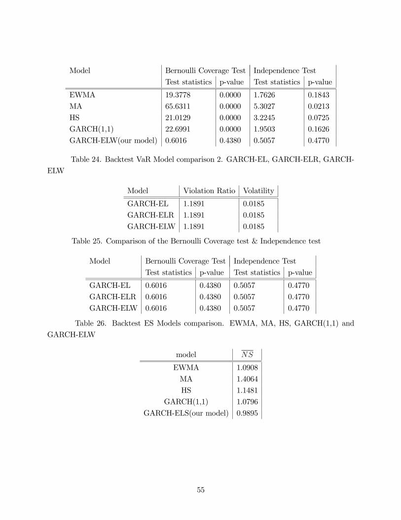
Model Bernoulli Coverage Test Independence Test

Test statistics p-value Test statistics p-value

EWMA 19.3778 0.0000 1.7626 0.1843

MA 65.6311 0.0000 5.3027 0.0213

HS 21.0129 0.0000 3.2245 0.0725

GARCH(1,1) 22.6991 0.0000 1.9503 0.1626

GARCH-ELW(our model) 0.6016 0.4380 0.5057 0.4770

Table 24. Backtest VaR Model comparison 2. GARCH-EL, GARCH-ELR, GARCH-

ELW

Model Violation Ratio Volatility

GARCH-EL 1.1891 0.0185

GARCH-ELR 1.1891 0.0185

GARCH-ELW 1.1891 0.0185

Table 25. Comparison of the Bernoulli Coverage test & Independence test

Model Bernoulli Coverage Test Independence Test

Test statistics p-value Test statistics p-value

GARCH-EL 0.6016 0.4380 0.5057 0.4770

GARCH-ELR 0.6016 0.4380 0.5057 0.4770

GARCH-ELW 0.6016 0.4380 0.5057 0.4770

Table 26. Backtest ES Models comparison. EWMA, MA, HS, GARCH(1,1) and

GARCH-ELW

model NS

EWMA 1.0908

MA 1.4064

HS 1.1481

GARCH(1,1) 1.0796

GARCH-ELS(our model) 0.9895

55

Figure 1: E¢ ciency comparison, Empirical CDF v.s. Normalized CDF

­5 ­4 ­3 ­2 ­1 0 1 2 3 4 5­0.2

­0.15

­0.1

­0.05

0

0.05

xStandard Normal distribution

C(x

)

­5 ­4 ­3 ­2 ­1 0 1 2 3 4 5­0.2

­0.15

­0.1

­0.05

0

0.05

xStandardized Mixed­Normal distribution

C(x

)

­5 ­4 ­3 ­2 ­1 0 1 2 3 4 5­0.2

­0.15

­0.1

­0.05

0

xStandardized t distribution with 5 degree of freedom

C(x

)

­5 ­4 ­3 ­2 ­1 0 1 2 3 4 5­0.1

0

0.1

0.2

0.3

xStandardized Chi­square distribution with 6 degree of freedom

C(x

)

56

Figure 2: Overlay of two estimators using iid errors: EmpiricalCDF v.s. EL-weighted CDF. N=500.

.

­2 0 2 4 6 8 100

0.2

0.4

0.6

0.8

1

1.2

1.4

xStandardized Chi­square distribution with 6 degree of freedom

F(x

)

Empirical CDFEL­weighted CDFTheoretical CDF

­8 ­6 ­4 ­2 0 2 4 6 8 100

0.2

0.4

0.6

0.8

1

1.2

1.4

xStandardized t­distribution with 9 degree of freedom

F(x

)

Empirical CDFEL­weighted CDFTheoretical CDF

­5 ­4 ­3 ­2 ­1 0 1 2 3 4 50

0.2

0.4

0.6

0.8

1

1.2

1.4

xStandard normal distribution

F(x

)

Empirical CDFEL­weighted CDFTheoretical CDF

­3 ­2 ­1 0 1 2 30

0.2

0.4

0.6

0.8

1

1.2

1.4

xStandardized mixed­normal distribution

F(x

)

Empirical CDFEL­weighted CDFTheoretical CDF

57

Figure 3: Overlay of two estimators using GARCH errors: Empirical CDF v.s. EL-weighted CDF.N=500.

­8 ­6 ­4 ­2 0 2 4 6 8 100

0.2

0.4

0.6

0.8

1

1.2

1.4

xStandardized Chi­square distribution with 6 degree of freedom

F(x

)

Empirical CDFEL­weighted CDFTheoretical CDF

­8 ­6 ­4 ­2 0 2 4 6 80

0.2

0.4

0.6

0.8

1

1.2

1.4

xStandardized t­distribution with 9 degree of freedom

F(x

)

Empirical CDFEL­weighted CDFTheoretical CDF

­10 ­5 0 50

0.2

0.4

0.6

0.8

1

1.2

1.4

xStandard normal distribution

F(x

)

Empirical CDFEL­weighted CDFTheoretical CDF

­4 ­3 ­2 ­1 0 1 2 3 4 50

0.2

0.4

0.6

0.8

1

1.2

1.4

xStandardized mixed­normal distribution

F(x

)

Empirical CDFEL­weighted CDFTheoretical CDF

58

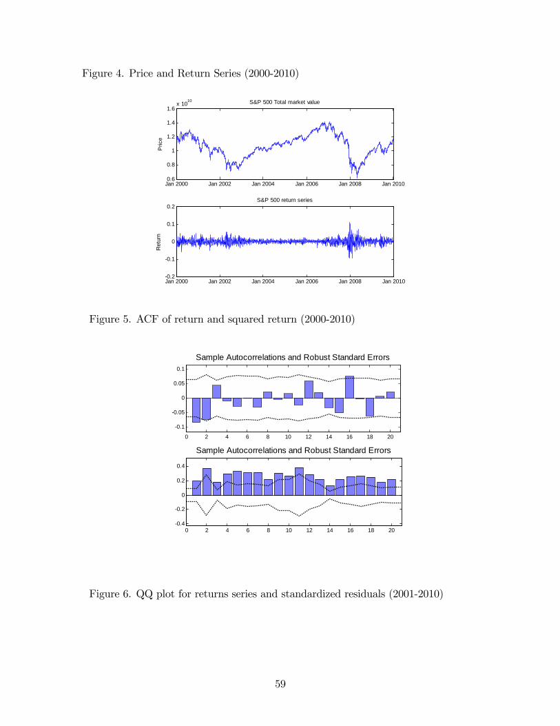
Figure 4. Price and Return Series (2000-2010)

Jan 2000 Jan 2002 Jan 2004 Jan 2006 Jan 2008 Jan 20100.6

0.8

1

1.2

1.4

1.6x 1010 S&P 500 Total market value

Pric

e

Jan 2000 Jan 2002 Jan 2004 Jan 2006 Jan 2008 Jan 2010­0.2

­0.1

0

0.1

0.2S&P 500 return series

Ret

urn

Figure 5. ACF of return and squared return (2000-2010)

0 2 4 6 8 10 12 14 16 18 20

­0.1

­0.05

0

0.05

0.1

Sample Autocorrelations and Robust Standard Errors

0 2 4 6 8 10 12 14 16 18 20­0.4

­0.2

0

0.2

0.4

Sample Autocorrelations and Robust Standard Errors

Figure 6. QQ plot for returns series and standardized residuals (2001-2010)

59

­4 ­3 ­2 ­1 0 1 2 3 4­0.1

­0.05

0

0.05

0.1

0.15

Standard Normal Quantiles

Qua

ntile

s of

 Inpu

t Sam

ple

QQ Plot of Sample Data versus Standard Normal

­4 ­3 ­2 ­1 0 1 2 3 4­10

­5

0

5

Standard Normal Quantiles

Qua

ntile

s of

 Inpu

t Sam

ple

QQ Plot of Sample Data versus Standard Normal

Figure 7. Conditional VaR and ES of model GARCH-ELW

Jan 2000 Jan 2002 Jan 2004 Jan 2006 Jan 2008 Jan 20100

0.05

0.1

0.15

0.2Conditional VaR (model­ELW)

VaR

VaR(alpha=0.05)VaR(alpha=0.01)

Jan 2000 Jan 2002 Jan 2004 Jan 2006 Jan 2008 Jan 20100

0.05

0.1

0.15

0.2Conditional ES (model­ELW)

ES

ES(alpha=0.05)ES(alpha=0.01)

Figure 8. Returns, Conditional Var and Conditional ES(2000-2010)

60

Jan 2000 Jan 2002 Jan 2004 Jan 2006 Jan 2008 Jan 2010­0.1

­0.05

0

0.05

0.1

0.15

0.2

0.25Return,VaR and ES (model=GARCH­ELW,alpha=0.01)

returnconditional VaR3conditional ES3

Figure 9. Backtest VaR model comparison 1. EWMA, MA, HS, GARCH(1,1) and

GARCH-ELW (2003-2010). (a) Returns and VaR for the whole sample

Dec 2003 Dec 2004 Dec 2005 Dec 2006 Dec 2007 Dec 2008 Dec 2009 Dec 2010­0.1

­0.05

0

0.05

0.1

0.15

Vol

atili

ty

Backtest VaR 1 (alpha=0.01)

returnEWMAMAHSGARCH(1,1)ELW

beginning of Greek debt crisis

first bailout loanbankruptcy of Lehman Brothers

(b) Focus on Sep 2008 to Dec 2008 � bankruptcy of Lehman Brothers

61

Sep 2008 Oct 2008 Nov 2008 Dec 2008­0.1

­0.05

0

0.05

0.1

0.15

VaR

backtest VaR (Sep 2008 to Dec 2008)(alpha=0.01)

returnEWMAMAHSGARCH(1,1)GARCH­ELW

Figure 10. Backtest VaR model comparison 2. GARCH-EL, GARCH-ELR,GARCH-

ELW(2003-2010)

Dec 2003 Dec 2004 Dec 2005 Dec 2006 Dec 2007 Dec 2008 Dec 2009 Dec 2010­0.1

­0.05

0

0.05

0.1

0.15

Vol

atili

ty

Backtest VaR 2 (alpha=0.01)

returnGARCH­ELGARCH­ELRGARCH­ELW

bankruptcy of Lehman Brothers

beginning of Greek debt crisis

first bailout loan

Figure 11. Backtest ES model comparison. EWMA, MA, HS, GARCH(1,1) and

GARCH-ELW(2003-2010). (a) Returns and ES for the whole sample

62

Dec 2003 Dec 2004 Dec 2005 Dec 2006 Dec 2007 Dec 2008 Dec 2009 Dec 2010­0.1

­0.05

0

0.05

0.1

0.15

0.2

0.25

Vol

atili

ty

backtest ES(alpha=0.01)

returnEWMAMAHSGARCH(1,1)GARCH­ELW bankruptcy of Lehman Brothers

beginning of Greek debt crisis

first bailout loan

(b) Focus on Sep 2008 to Dec 2008 � bankcruptcy of Lehman Brothers

Sep 2008 Oct 2008 Nov 2008 Dec 2008­0.1

­0.05

0

0.05

0.1

0.15

0.2

0.25

ES

backtest ES (Sep 2008 to Dec 2008)(alpha=0.01)

returnEWMAMAHSGARCH(1,1)GARCH­ELW

63