
Efficient Algorithms for Locating Maximum Average Consecutive Substrings
37
Efficient Algorithms for Locating Maximum Average Consecutive Substrings Jie Zheng Department of Computer Science UC, Riverside
description
Efficient Algorithms for Locating Maximum Average Consecutive Substrings. Jie Zheng Department of Computer Science UC, Riverside. Outline. Problem Definition Applications to Molecular Biology Two Existing Algorithms Open Problems. Definition of Problem. - PowerPoint PPT Presentation
Transcript of Efficient Algorithms for Locating Maximum Average Consecutive Substrings

Efficient Algorithms for Locating Maximum Average
Consecutive Substrings
Jie Zheng
Department of Computer Science
UC, Riverside

Outline
• Problem Definition
• Applications to Molecular Biology
• Two Existing Algorithms
• Open Problems
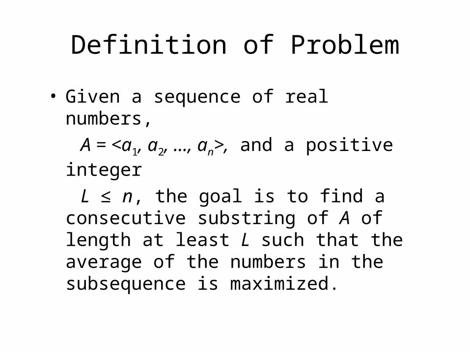
Definition of Problem
• Given a sequence of real numbers,
A = <a1, a2, …, an>, and a positive integer
L ≤ n, the goal is to find a consecutive substring of A of length at least L such that the average of the numbers in the subsequence is maximized.
Applications in Biology
• Locating GC-rich Regions
• Post-Processing Sequence Alignments
• Annotating Multiple Sequence Alignments
• Computing Ungapped Local Alignments with Length Constraints
Two Existing Algorithms
• An O(nlogL)-time Algorithm (Yaw Ling Lin, Tao Jiang, Kun-Mao Chao, 200
1)
• A Linear Time Algorithm for Binary Strings
(Hsueh-I Lu, 2002)
The O(nlogL)-time Algorithm(Yaw-Ling Lin, Tao Jiang, Kun-Mao Chao,2001)
Basic Scheme:
• Finding good partner of each element,
i.e. for element ai, locate aj, such that the segment <ai,…, aj> has maximum average among all substrings starting from ai.
• Choose the <ai,…, aj> with the maximum average among the n candidates.
Important Concepts
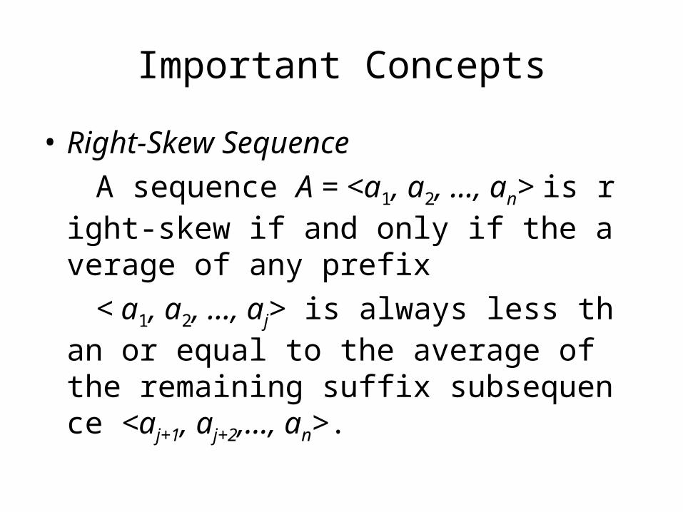
• Right-Skew Sequence
A sequence A = <a1, a2, …, an> is right-skew if and only if the average of any prefix
< a1, a2, …, aj> is always less than or equal to the average of the remaining suffix subsequence <aj+1, aj+2,…, an>.
Important Concept
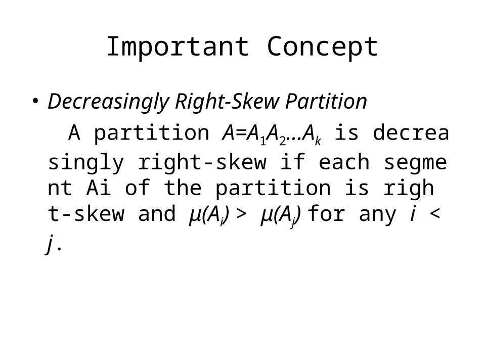
• Decreasingly Right-Skew Partition
A partition A=A1A2…Ak is decreasingly right-skew if each segment Ai of the partition is right-skew and μ(Ai) > μ(Aj) for any i < j.
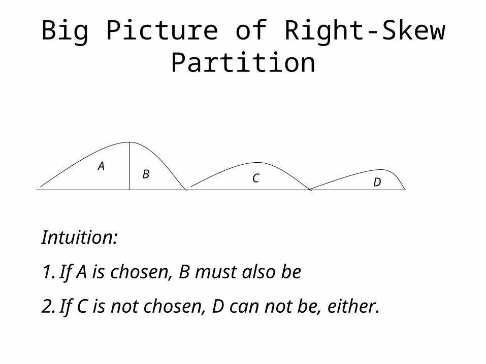
Big Picture of Right-Skew Partition
AB C D
Intuition:
1. If A is chosen, B must also be
2. If C is not chosen, D can not be, either.

Lemma 7(Huang): The Maximum Average Substring
Can not be longer than 2L-1
• Proof If C is the maximum average substring with length ≥2L, let C= AB, where |A|≥L and |B|≥L, then the average of A or B is no less than that of C.
Say μ(A) > μ(B), then μ(A) > μ(AB)
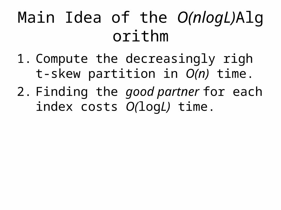
Main Idea of the O(nlogL)Algorithm
1. Compute the decreasingly right-skew partition in O(n) time.
2. Finding the good partner for each index costs O(logL) time.
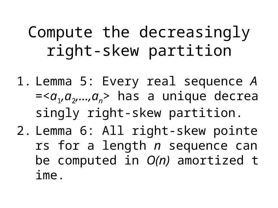
Compute the decreasingly right-skew partition
1. Lemma 5: Every real sequence A=<a1,a2,…,a
n> has a unique decreasingly right-skew partition.
2. Lemma 6: All right-skew pointers for a length n sequence can be computed in O(n) amortized time.
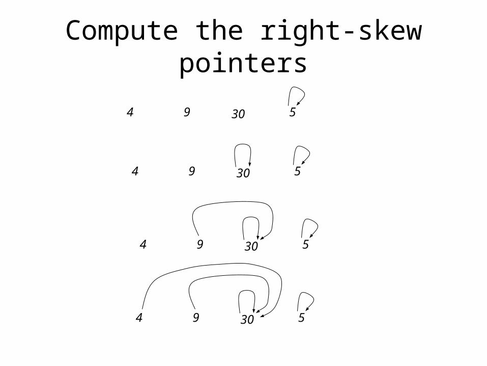
Compute the right-skew pointers
4 9 30 5
4 9 30 5
4 9 30 5
4 9 30 5
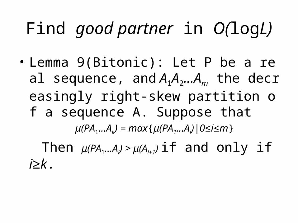
Find good partner in O(logL)
• Lemma 9(Bitonic): Let P be a real sequence, and A1A2…Am the decreasingly right-skew partition of a sequence A. Suppose that
μ(PA1…Ak) = max{μ(PA1…Ai)|0≤i≤m}
Then μ(PA1…Ai) > μ(Ai+1) if and only if i≥k.

What does Lemma 9 tell us?
• Locating good partner can be done with binary search!
To find k so that
μ(PA1…Ak) = max{μ(PA1…Ai)|0 ≤ i ≤ m}
We guess i and make it closer to k:
1. μ(PA1…Ai) >μ(Ai+1) implies i ≥ k
2. μ(PA1…Ai) ≤μ(Ai+1) implies i < k
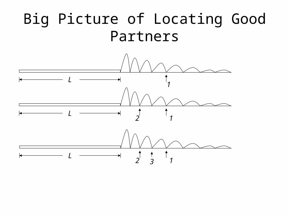
Big Picture of Locating Good Partners
L1
L12
L12 3

Date Structure for Binary Search
logL Pointer-Jumping Tables• j (k) denotes the right end-point of the kth right-ske
w segment .• p (0)[i] = p[i], where p[i] is right-skew pointer for i,
p (k+1) [i] = min{p (k) [p (k) [i]+1], n}. 1 k logL • The precomputation of the jumping tables takes at
most O(nlogL) time.
• Totally n phases
• Each phase costs O(logL)
• Overall: O(nlogL)-time
The Time Complexity

Crying Out
for A Linear Time Algorithm!!
A Linear-Time Algorithm for Binary Strings (Hsueh-I Lu, 2002)
• Build upon the previous algorithm• Improvements: - Considering an upper bound on the number of
right-skew segments - Working simultaneously on the right-skew
partitions of forward and reverse strings - Utilizing Properties of Binary Strings
Basic Scheme
Let B = log3n and b = (loglogn)3 1. Choose O(n/ logn) indices i of S such that if g(i)-i
B holds for any of such i, then g(i) can be found in O(logn) time.
2. Choose O(n/ loglogn) indices i of S such that if B g(i) – i b holds for any of such i, then g(i) can be found in O(loglogn) time.
3. Find g(i) for all indices i such that g(i) – i b.
Denotations• A right-skew decompostion of any substring S [p,
q] is a nonempty set of i indices i1,i2,…, il so that S[i
1,i2], S[i2, i3],…, S[il-1, il] are decreasingly right-skew partition of S.
• Let DS (i, j) denote the right-skew decomposition of S[i, j]
• If P = {p1, p2 ,…, pk, pk+1}, where p1< p2<…<pk+1, then
),()( 11
ii
k
iSS ppDPD
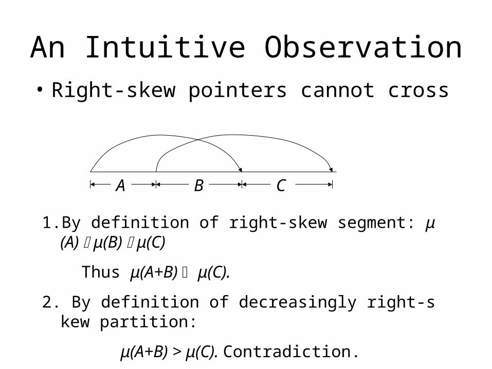
An Intuitive Observation• Right-skew pointers cannot cross
A B C
1. By definition of right-skew segment: μ(A) μ(B) μ(C)
Thus μ(A+B) μ(C).
2. By definition of decreasingly right-skew partition:
μ(A+B) > μ(C). Contradiction.

The Big Picture of Right-Skew Decomposition

Lemma 3: from the big picture
• If j DS (P), then DS (j, n) DS (P).
Lemma 3 tells us that if j belongs to the right-skew decomposition of some set of indices, then its good partner will also be. Thus, we only need to search for its good partner among a limited number of indices.
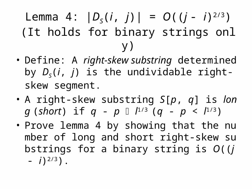
Lemma 4: |DS(i, j)| = O((j - i)2/3)(It holds for binary strings only)
• Define: A right-skew substring determined by DS(i, j) is the undividable right-skew segment.
• A right-skew substring S[p, q] is long (short) if q - p l1/3 (q - p < l1/3)
• Prove lemma 4 by showing that the number of long and short right-skew substrings for a binary string is O((j - i)2/3).
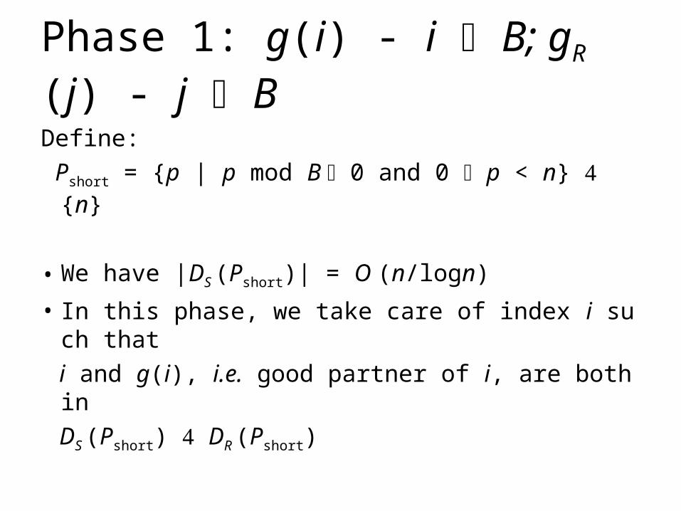
Phase 1: g(i) - i B; gR(j) - j B
Define:
Pshort = {p | p mod B 0 and 0 p < n} {n}
• We have |DS (Pshort)| = O (n/logn)
• In this phase, we take care of index i such that
i and g(i), i.e. good partner of i, are both in
DS (Pshort) DR (Pshort)
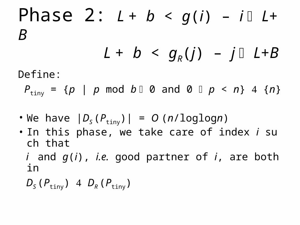
Phase 2: L + b < g(i) – i L+B L + b < gR(j) – j L+B
Define:
Ptiny = {p | p mod b 0 and 0 p < n} {n}
• We have |DS (Ptiny)| = O (n/loglogn)• In this phase, we take care of index i such that i and g(i), i.e. good partner of i, are both in
DS (Ptiny) DR (Ptiny)

Phase 3: g(i)-i L+b, gR(j)-j L+b
• We set up a table M whose (x,y) entry contains the index z, such that:
If C is a binary string of L+b bits, x is the number of ‘1’ in the first L bits of C; y is the binary string consisting of the last b bits of C; z is the good partner of index 0 in C.
Because b is relatively small, the number of possible value for x and y is linear
• Looking up the table M, we can cope with the left-over case in O(n)-time.

Open Problems:
How to extend the linear time algorithm for binary strings to arbitrary strings.

INTERESTED?
Contact: Jie Zheng
Department of Computer Science Surge Building # 350
UC, Riverside E-mail: [email protected]