Efficiency of Analytical Methodologies in Uncertainity Analysis of Seismic Core Damage Frequency

8/12/2019 Efficiency of Analytical Methodologies in Uncertainity Analysis of Seismic Core Damage Frequency

http://slidepdf.com/reader/full/efficiency-of-analytical-methodologies-in-uncertainity-analysis-of-seismic 1/16



Journal of Power and Energy Systems

Vol. 6, No. 3, 2012

380

2. Analytical Methods to Evaluate Seismic Core Damage Frequency

2.1 Generic Procedure for All Methods

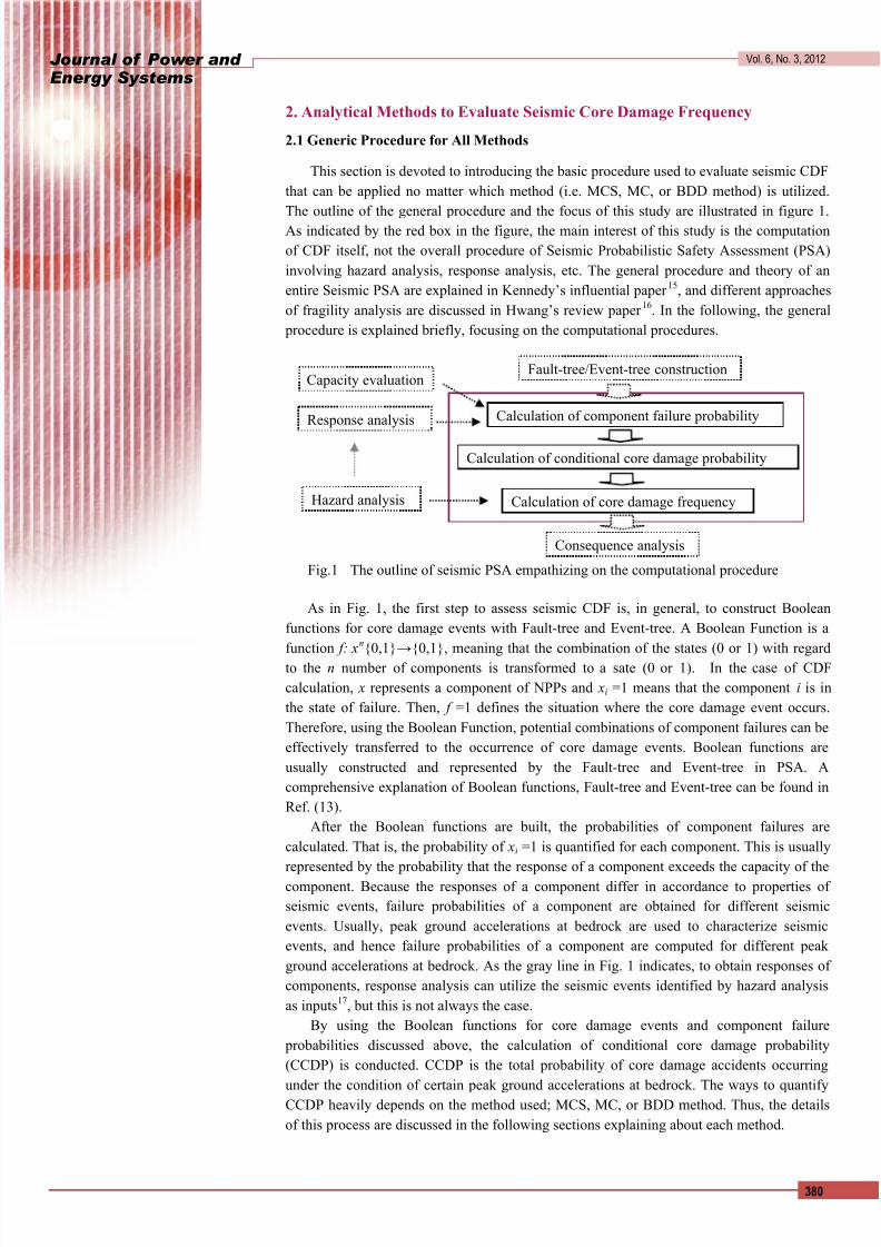
This section is devoted to introducing the basic procedure used to evaluate seismic CDF

that can be applied no matter which method (i.e. MCS, MC, or BDD method) is utilized.

The outline of the general procedure and the focus of this study are illustrated in figure 1.As indicated by the red box in the figure, the main interest of this study is the computation

of CDF itself, not the overall procedure of Seismic Probabilistic Safety Assessment (PSA)

involving hazard analysis, response analysis, etc. The general procedure and theory of an

entire Seismic PSA are explained in Kennedy’s influential paper 15

, and different approaches

of fragility analysis are discussed in Hwang’s review paper 16

. In the following, the general

procedure is explained briefly, focusing on the computational procedures.

As in Fig. 1, the first step to assess seismic CDF is, in general, to construct Boolean

functions for core damage events with Fault-tree and Event-tree. A Boolean Function is a

function f: x

n

{0,1}→

{0,1}, meaning that the combination of the states (0 or 1) with regardto the n number of components is transformed to a sate (0 or 1). In the case of CDF

calculation, x represents a component of NPPs and xi =1 means that the component i is in

the state of failure. Then, f =1 defines the situation where the core damage event occurs.

Therefore, using the Boolean Function, potential combinations of component failures can be

effectively transferred to the occurrence of core damage events. Boolean functions are

usually constructed and represented by the Fault-tree and Event-tree in PSA. A

comprehensive explanation of Boolean functions, Fault-tree and Event-tree can be found in

Ref. (13).

After the Boolean functions are built, the probabilities of component failures are

calculated. That is, the probability of xi =1 is quantified for each component. This is usually

represented by the probability that the response of a component exceeds the capacity of thecomponent. Because the responses of a component differ in accordance to properties of

seismic events, failure probabilities of a component are obtained for different seismic

events. Usually, peak ground accelerations at bedrock are used to characterize seismic

events, and hence failure probabilities of a component are computed for different peak

ground accelerations at bedrock. As the gray line in Fig. 1 indicates, to obtain responses of

components, response analysis can utilize the seismic events identified by hazard analysis

as inputs17

, but this is not always the case.

By using the Boolean functions for core damage events and component failure

probabilities discussed above, the calculation of conditional core damage probability

(CCDP) is conducted. CCDP is the total probability of core damage accidents occurring

under the condition of certain peak ground accelerations at bedrock. The ways to quantifyCCDP heavily depends on the method used; MCS, MC, or BDD method. Thus, the details

of this process are discussed in the following sections explaining about each method.

Fault-tree/Event-tree construction

Hazard analysis

Calculation of component failure probabilityResponse analysis

Capacity evaluation

Calculation of conditional core damage probability

Calculation of core damage frequency

Consequence analysis

Fig.1 The outline of seismic PSA empathizing on the computational procedure




Vol. 6, No. 3, 2012

381

Finally, seismic CDF is computed by integrating CCDP with seismic hazard curves.

Seismic CDF F CD is expressed by the following equation for all methods in this paper.

( )0

( )CD CD

d d

d

H F P

α α α

α

∞ = −

∫ (1)

where P CD(α) is CCDP at the given peak ground acceleration level α, and H (α) is a seismic

hazard curve which defines the frequencies of seismic events at the acceleration level α.

2.2 Minimal Cut Set Based method

MCS method is the traditional and still most commonly used method to calculate CCDP

in seismic PSA. In the PSA, MCS is a set of minimal combinations of component failures,

which can cause the occurrence of an unwanted event, such as a core damage accident.

Because of its nature, MCS itself is a very useful tool to review and document a PSA model.

However, quantifying CCDP from MCS (i.e. MCS method) requires some form of

approximation.

First, in order to obtain CCDP with MCS method, it is required to convert the Boolean

functions into MCS. Then, the failure probability P x(α) of each component x in MCS is

quantified with the assumption that the capacity and response of components are

log-normally distributed as in Eq. (2) 14,18,

.

( ) ( )2 2

ln ( ) ln( ) x

R S

R S P

α α

β β

− = Φ

+

(2)

where, Ф denotes cumulative distribution function for the standard normal distribution, S is

the median value for the capacity of the component, and ( ) R α indicates median value for the

response of the component given ground acceleration α. β R and β S express logarithmicstandard deviations of R and S respectively. The right hand side of Eq. (2) is equivalent to

the probability that R exceeds S . By using component failure probabilities P x(α), the

probability of MCS P MCS (α) is obtained simply by multiplying all P x(α) in a minimal cut as

in P MCS (α)=Π[ P x(α)].

After getting P MCS (α), some approximations are required to compute CCDP. In seismic

PSA, Upper Bound Approximation (UBA) method is generally applied because other

approximation methods are less accurate or can exceed computational limits. Accordingly,

this study utilizes UBA method. The UBA method can be expressed with the total number

of MCS k as the following.

1( ) 1 1 ( )

k

T MCS

i P P α α

== − − ∏ (3)

Eq. 3 can be directly utilized to obtain CCDP if the core damage event is expressed by only

one Fault-tree. But normally, the core damage event is expressed with several accident

sequences by using Event-trees. In that case, with the total number, L, of accident sequences

resulting in core damage states, CCDP P CD(α) is expressed as in Eq. (3)'.

1

( ) j

L

CD T j

P P α =

= ∑ (3)'

CCDP P CD(α) obtained from Eqs. (3) and (3)' is accurate if and only if all k MCS are

independent from each other. However, this rarely happens in a practical PSA study andhence the effect of the approximation needs to be examined carefully.




Vol. 6, No. 3, 2012

382

With the procedures discussed above and together with Eq. (1), the approximated mean

value of CDF can be estimated by MCS method. However, to obtain uncertainty of CDF, it

is necessarily to propagate uncertainty corresponding to capacity and response of

components to CDF. To do so, the uncertainties are divided into two factors; uncertainty due

to randomness and uncertainty derived from the lack of knowledge. Accordingly,

logarithmic standard deviation of response and capacity are expressed as β R2

= β Rr

2

+ β Ru

2

, β S

2= β Sr

2+ β Su

2, where β Rr stems from randomness and β Ru is from the lack of knowledge. By

modifying equations appearing in Ref. (14) with those parameters and non-exceeding

probability level Z , Eq. (2) can be expressed as the following for uncertainty analysis.

( ) ( ) 1 2 2

2 2

ln ( ) ln ( )( )

Ru Su

x

Rr Sr

R S Z P

α β β α

β β

− − + Φ + = Φ +

(4)

It is worth noticing that mean value of Eq. (4) is mathematically equivalent to the value of

Eq. (3) 18

.

2.3 Monte Carlo method

In MC method, CCDP is assessed directly from the Boolean functions constructed with

Fault-tree and Even-tree by means of Monte Carlo simulation. Unlike MCS method, this

method does not need to use any approximation techniques, and hence this method holds

certain accuracy in assessing CCDP or CDF, except for random number errors.

The method is conducted as the following. First, each component is determined to be 1

(failure) or 0 (intact) according to their failure probabilities such as in Eq. (2). Then, if core

damage happens in the component configuration, it is counted and stored as the number of

core damage events occurring. Finally, CCDP is calculated simply by dividing the counted

total number of times that core damage occurs in the simulation by the total iteration

number in the simulation.

As it could be realized from this procedure, MC method does not need to calculate the

failure probabilities of components to quantify CCDP. Instead, all that is required is

deciding whether the component is categorized as failure or intact during the trial of the

simulation. Thus, instead of Eq. (2), the following equation can be utilized.

1 if R >SQ (R ,S )

0 otherwise

i ii i i

=

(5)

where, Qi =1 means that the component fails in the trial i, and R i and Si represent the

response and capacity respectively in the trial. The values for the component response and

capacity are in turn obtained with normally distributed random number Y : R i= R exp( β R Yi),Si= S exp( β S Yi). Note that with these equations, random numbers are generated separately

for response and capacity, and hence correlations of response and capacity among

components can be arbitrarily considered. Also, unlike other methods, the correlations can

be considered in point estimation as well as uncertainty analysis by MC method. This

particular approach for seismic CDF calculation was introduced as DQFM method12

and it

is used in this paper. After calculating CCDP with these procedures, Eq. (1) is used to obtain

CDF.

For uncertainty analysis, uncertainties of response and capacity are divided into

uncertainties due to randomness and epistemic inadequacy in the same way as with MCS

method. That is, R i= R exp( β Rr Yi+ β RuYi), Si= S exp( β Sr Yi+ β SuYi), where each Yi represents

different random numbers and assumed to be independent from each other. Then, M timessimulation conducted by sampling Yi for randomness ( β Rr and β Sr ) and by holding the same




Vol. 6, No. 3, 2012

383

values for epistemic insufficiency ( β Ru and β Su) are performed N times by changing the

values of epistemic insufficiency.

Therefore, while other methods can conduct uncertainty analysis only by N times

computations (O( N )), MC method needs to have M by N steps (O( M N )). Another

disadvantage of this method is that it contains random number errors, which become

relatively high when very low probabilities contribute to the outcome of the computation.For this problem, dagger sampling was utilized

19. However, for seismic CDF any special

treatments for the problem would not be required because failure probabilities of

components contributing to seismic CDF are likely to be high enough.

2.4 Binary Decision Diagram method

Binary Decision Diagram (BDD) is a well-known representation of Boolean functions,

among others such as truth table, Karnaugh map, Ternary vector list, or Boolean Neural

Networks. Compared to other representations, BDD representation has significant

advantages in computing probability over Boolean functions. More concretely, exact CCDP

and CDF can be obtained by BDD without any approximation (MCS method) and randomnumber error (MC method) within a reasonable amount of time.

The first step of BDD method is to build BDD from a Boolean function by recursively

applying Shannon decomposition to variables of the function. Let F denote a Boolean

function of x among others, then

[ 1] [ 0] F xF x x F x′= ← + ← (6)

To illustrate how this step is conducted more concretely, let's assume that there are three

variables, x1, x2, and x3, all connected by the "OR" gate as shown in the far left of Fig. 2. If

variable ordering is x1 < x2 < x3, the first thing to do is to construct BDD with x1 and x2 (this

means that the algorithm "Apply" proposed in Ref. (20) is utilized). Then, using Eq. (6) and

some reduction rules, BDD for x1 "OR" x2 is built as in the middle of Fig. 2. Finally, theconstructed BDD and x3 are considered with connectivity "OR", and by applying Eq. (6),

BDD which looks like the right side of Fig. 2 is generated.

Fig. 2 An image of the BDD construction scheme

Calculating probability through BDD is relatively straightforward. Because BDD can

be expressed by Eq. (6), the probability of F is P ( F )= P ( x) P ( F [ x←1])+ P ( x') P ( F [ x←0]). For

P ( x), Eq. (2) is applied in point estimation and P ( x') is simply 1- P ( x). In uncertainty

analysis, Eq. (4) is utilized as in MCS method. Like other methods, with CCDP obtained by

using the above procedures, Eq. (1) is used to quantify CDF, but unlike other methods, CDF

assessed by this method is an exact solution.

However, a major problem of BDD method is that it is not always possible to construct

BDD from Boolean functions. This is because building BDD takes a lot of memory space,

especially when Boolean functions, or a PSA model, are too big, such as the one from the

nuclear industry as it is demonstrated in Table 7.4 of Ref. (13). Moreover, the size of BDD

heavily depends on the processing order of Boolean functions' variables, and finding the best order is a NP-hard problem

11. Therefore, a number of researchers have developed

F

x1 x2 x30 1

x1

x2

0 1

x1

x2

x3

x3

0 1

OR(OR)

10

10

10

0

1

1

1

0

0




Vol. 6, No. 3, 2012

384

heuristics to find a reasonable order of variables. Though, it is not yet certain that BDD

method can be used in all PSA models. Given this status of BDD method, several

approximation methods were proposed to make sure that BDD could be made for all cases

21.

Summarizing discussions about different methods, while MCS method may not obtain

accurate values of CDF, MC and BDD methods are potentially able to do so. However, CDFquantified from MC method contains random number errors, and it would take a long time

for uncertainty analysis. On the other hand, BDD method cannot always be utilized,

depending on the structure of the PSA model, variable ordering, and selected heuristics.

3. Calculations and Results

3.1 The Model

The purpose of this study is to examine the efficiencies of analytical methods, instead

of assessing the risk at a specific NPP. Given that objective, a hypothetical BWR plant PSA

model22

is utilized in this study because the model has been well examined and

documented8,9,12. This model consists of five initiating events and mitigation systems to ease

accident progression induced by the initiating events.

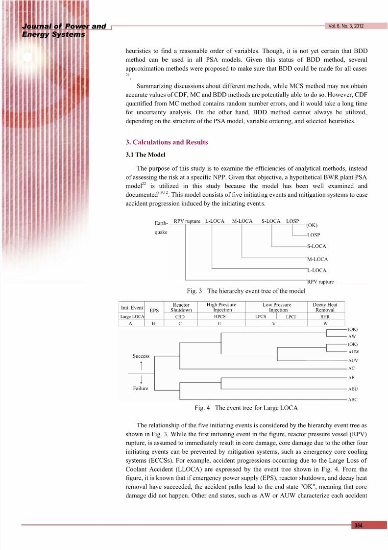
Fig. 3 The hierarchy event tree of the model

Fig. 4 The event tree for Large LOCA

The relationship of the five initiating events is considered by the hierarchy event tree as

shown in Fig. 3. While the first initiating event in the figure, reactor pressure vessel (RPV)

rupture, is assumed to immediately result in core damage, core damage due to the other four

initiating events can be prevented by mitigation systems, such as emergency core cooling

systems (ECCSs). For example, accident progressions occurring due to the Large Loss of

Coolant Accident (LLOCA) are expressed by the event tree shown in Fig. 4. From the

figure, it is known that if emergency power supply (EPS), reactor shutdown, and decay heat

removal have succeeded, the accident paths lead to the end state "OK", meaning that core

damage did not happen. Other end states, such as AW or AUW characterize each accident

Init. Event

Large LOCA

A

EPS

B

ReactorShutdown

CRD

C

High Pressure Injection

Low PressureInjection

HPCS LPCS LPCI

U V

Decay HeatRemoval

RHR

W

Success

Failure

(OK)

(OK)

AW

AUW

AUV

AC

AB

ABU

ABC

RPV rupture L-LOCA M-LOCA S-LOCA LOSP(OK)

LOSP

S-LOCA

M-LOCA

L-LOCA

RPV rupture

Earth-

quake




Vol. 6, No. 3, 2012

385

scenario that results in core damage. For instance, because "A" indicates LLOCA initiating

event and "W" represents the failure of the residual heat removal (RHR) system, the

accident sequence "AW" is an accident sequence where core damage happens due to the

occurrence of LLOCA and the malfunction of RHR. The meanings of each character used in

the end states or labels for all initiating events are shown in Table 1. Hereinafter, accident

sequences will be indicated by the labels in accordance with Table 1.It was discussed above that if certain mitigation systems function properly, in some

cases core damage can be avoided. In turn, whether or not mitigation systems can function

to stop accident progressions depends on whether components consisting of mitigation

systems can function or not. This dependency of mitigation systems on components is

expressed by a Fault-tree. The Fault-tree is composed of 125 components, 66 'OR' gates,

and 24 'AND' gates. The details of the Fault-tree and the parameters for component failure

probabilities used in this study can be found in Ref. (22).

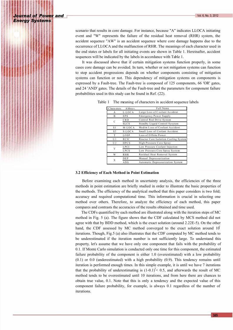
Table 1 The meaning of characters in accident sequence labels

3.2 Efficiency of Each Method in Point Estimation

Before examining each method in uncertainty analysis, the efficiencies of the three

methods in point estimation are briefly studied in order to illustrate the basic properties of

the methods. The efficiency of the analytical method that this paper considers is two fold;

accuracy and required computational time. This information is crucial in selecting one

method over others. Therefore, to analyze the efficiency of each method, this paper

compares and contrasts the accuracies of the results obtained and time used.

The CDFs quantified by each method are illustrated along with the iteration steps of MC

method in Fig. 5 (a). The figure shows that the CDF calculated by MCS method did not

agree with that by BDD method, which is the exact solution (around 2.22E-5). On the other

hand, the CDF assessed by MC method converged to the exact solution around 107

iterations. Though, Fig.5 (a) also illustrates that the CDF computed by MC method tends to

be underestimated if the iteration number is not sufficiently large. To understand this

property, let's assume that we have only one component that fails with the probability of

0.1. If Monte Carlo simulation is conducted only one time for this component, the estimated

failure probability of the component is either 1.0 (overestimated) with a low probability

(0.1) or 0.0 (underestimated) with a high probability (0.9). This tendency remains until

iteration is performed enough times. In this simple example, it is until we have 7 iterations

that the probability of underestimating is (1-0.1)7< 0.5, and afterwards the result of MC

method tends to be overestimated until 10 iterations, and from here there are chances to

obtain true value, 0.1. Note that this is only a tendency and the expected value of this

component failure probability, for example, is always 0.1 regardless of the number of

iterations.

C hara cters A bbre v.

A L-LO C A

B EP S

CR D

SLCS

S1 M -LO C A

S2 S-L O C A

T LO SP

U 1 RC IC

U 2 H P CS

LPCI

LPCS

W RH R

D E P

A D SX

High Pressure Core Spray

Low Pressure Coolant Injection

C

VLow Pressure Core Spray System

Residual Heat Removal System

Manual Depressurization

Automatic Depressurization System

Reactor Core Isolation Cooling System

Ful l Name

Medim L oss of Coolant Accident

Small Loss of Coolant Accident

Loss of O ffsite Power

Large Loss of C oolant Accident

Emergency Power Supply

Control Rod Drive System

Standby Liquid Control Sysytem




Vol. 6, No. 3, 2012

386

As another example, the occurrence frequency of sequence "S2UW" is shown in Fig. 5

(b). It is indicated in the figure that instead of overestimating, MCS method underestimated

the occurrence frequency. Even in this case, MC method converged to the exact solution

quantified by BDD method around 107 iterations.

(a) CDF (the sum of all sequences) (b) Sequence "S2UW"

Fig. 5 Occurrence frequency obtained by each method along with sample sizes

The consistency of MC method with BDD method also held true in the accident

sequence level as shown in Table 2. On the other hand, occurrence frequencies of some

accident sequences obtained by MCS method were 2 times more or 0.9 times less than those

assessed by BDD method. Therefore, by summarizing the above, it has been confirmed that

MC method is almost as accurate as BDD method, but MCS method is not likely to be

accurate enough in point estimation.

Table 2 The ratio of accident sequence occurrence frequencies to those by BDD method*

* The ratios of cells colored by gray are less than 90%, and the proportions of cells colored

by orange are more than 200%.

However, another important question is how long each method takes to obtain the

results with this degree of accuracy. For the experiment above, MCS and BDD methods

took 3.5 and 1.2 seconds respectively, while MC method spent 14,248 seconds. These times

were observed using a personal computer running Windows 7 with a processor speed of 3.1

GHz and 4 GB of RAM. Therefore, as far as this PSA study is concerned, BDD method

turned out to be the most efficient in point estimation in terms of accuracy and

computational time. But, as discussed in section 2.4, the main concern of BDD method is

not computational time, but time complexity and memory space, which varies from model

to model and variable ordering. Because the time complexity and required memory space

can exceed the computer’s resources, BDD simply cannot be constructed in some cases

while MC method is always applicable in theory. Therefore, the results above show that if

BDD is not applicable to a PSA study, one should think about the accuracy-time tradeoff to

select MC method or MCS method.

x

x

Iteration steps

F r e q u e n c y ( / r e a c t o r y e a r )

Iteration steps


RPV AW AUW AUV AC AB ABU ABC S1W

MCS 1.00 1.40 1.07 1.81 0.79 1.35 1.76 4.19 1.39

MC 0.97 1.01 1.00 1.01 1.01 1.00 1.00 1.00 1.01S1UW S1UV S1UX S1C S1B S1BU S1BC S2W S2U1W

MCS 1.09 1.73 0.92 0.82 1.33 1.78 3.89 1.28 1.43

MC 0.99 1.00 0.99 0.98 1.01 1.00 1.00 0.99 1.02

S2UW S2UV S2UX S2C S2B S2BU1 S2BU S2BC TW

MCS 0.75 1.11 1.20 0.87 1.31 1.36 1.96 3.42 1.22

MC 1.00 0.99 1.04 0.99 1.00 1.00 1.00 1.00 1.01

TU1W TUW TUV TUX TC TB TBU1 TBU TBC

MCS 1.30 0.92 1.20 1.16 1.25 1.22 1.23 1.75 2.62

MC 1.00 0.99 1.00 0.96 1.02 0.99 0.98 0.99 1.00

Accident Sequence

The Ratio of

Frequency

Accident Sequence

The Ratio of

Frequency

Accident Sequence

The Ratio of

Frequency

Accident Sequence

The Ratio of

Frequency




Vol. 6, No. 3, 2012

387

3.3 Efficiency of Each Method in Uncertainty Analysis

In order to study the efficiencies of MCS, MC and BDD methods in uncertainty

analysis, this section first compares CCDP curves, and then examines CDFs calculated with

two different hazard curves. The Monte Carlo simulation was conducted 105

times for MCSand BDD methods, and 10

5 by 10

4 times for MC method.

The comparison of CCDP curves computed by MCS, MC, and BDD methods is shown

in Fig. 6. The figure shows that the CCDP curves of MC method and BDD method highly

agreed with each other and that the curve of MCS deviated from others. More concretely,

the CCDP curves corresponding to 95%, 50%, 5% and the mean values were overestimated

by MCS method. In particular, the 95%, 50% and mean values of CCDP calculated by MCS

method exceeded 1.0 which should not go beyond 1.0 in theory. This happened because

each of the sequence occurrence probabilities (Eq. (3)), the sum of which is CCDP (Eq.

(3)'), can incorrectly reach up to 1.0 due to the overestimation of UBA method and the

imperfect handling of negation. Essentially, treating negation correctly can prevent this

bizarre phenomenon because the correct treatment of negation makes sure that all sequencesare mutually exclusive. But, of course, the treatment of negation is something that cannot be

done perfectly in the MCS method10

.

Fig. 6 CCDP curves: from the top to the bottom, 95%, 50%, and 5% values

are plotted with dotted lines and mean values are expressed with solid lines

In addition to the overall overestimation of the MCS method, the relationship of the

mean curve and the median (50%) curve obtained by MCS method turned out to be

different from the relationships computed by other methods. For MC and BDD methods, the

relationship changed only once; the mean curve is higher than the median curve until a

certain point (around 900 Gal), and afterward the mean curve becomes lower. The cross

point seems to be closely related to the point where the 95% curve reaches 1.0. This is

because the mean value can be higher than the median value when the right tail of the

distribution of CCDP is longer than the left side of the distribution, and because when the

95% curve reaches 1.0, the right tail of the distribution is more likely to be limited by the

value 1.0. On the other hand, the relationship of the mean and median curves for MCS

method changes twice instead of only once. The fist change occurs around 800 Gal when

the increment of 95% value starts decreasing and the second intersection appears when the

increment of the 95% value starts increasing again. The change on the increment of 95%

can happen twice because of the following reasons. As discussed above, the effect of the

probabilistic limitation (1.0) can take place on all accident sequences in MCS method,

0

0.2

0.4

0.6

0.8

1

1.2

1.4

1.6

1.8

2

0 500 1000 1500 2000

MCS method

MC method

BDD method

P r o b a b i l i t y

Ground Acceleration Level (Gal)




Vol. 6, No. 3, 2012

388

instead of only on a total CCDP. Therefore, when the 95% values of some sequences reach

1.0, the increment of 95% value decreases, but afterward the 95% values of other sequences

can increase rapidly at some larger ground acceleration levels, which resulted in the two

cross points of the mean and median curves.

For uncertainty analysis of CDFs, two calculation cases corresponding to different

hazard curves were considered. One of the curves was utilized to examine the efficienciesof all three methods. Another curve was employed as a hazard curve containing realistic

uncertainty information to compare the approximated results (by MCS method) and the

exact solutions (by BDD methods).

Fig. 7 The results of uncertainty analysis with the fist hazard curve

The first hazard curve utilized is the same one that was presented with the hypothetical

BWR plant PSA model in Ref. (22) and used in the point estimate calculation of the

previous section. The uncertainty of this hazard curve was represented by the logarithmicstandard deviation β =1.4 for all ground acceleration levels

22. The results of the uncertainty

analysis by MCS, MC and BDD methods are shown in Fig. 7 (a). As indicated in the figure,

the uncertainty ranges, or the 90% confidence intervals, took place within the order of 10-7

to around 10-4

for all methods. The comparison of results shows that the results of

uncertainty analysis of MC and BDD methods are consistent with each other, while that of

MCS again disagreed with the other two methods. However, the degree of deviation with

regard to the mean value by MCS method from the other methods was less compared with

that in the point estimate calculation; while the ratio of the mean value obtained by MCS

method to that by BDD method was 1.34 in the point estimation, the ratio became 1.17 in

the uncertainty analysis. This phenomenon can be explained by the fact that the

probabilities for each accident sequence cannot exceed 1.0 and hence the right tail of thedistribution for CDF cannot be overestimated as much as the value of point estimation. In

fact, although the exact same random numbers were used for MCS and BDD methods, Fig.

7 (b) shows that while intense variations towards unreasonably high values were occurring

in BDD method (around 102 iterations), it was not happening in MCS method, which

supports the argument above.

The mean values of CDFs reached the point of convergence around 104 iterations for all

MCS, MC, and BDD methods (Fig. 7 (b)). But, for MC method, in order to perform each of

104 iterations presented in Fig. 7 (b), it was required to conduct 10

5 iterations because MC

method utilizes Monte Carlo simulation to compute each value of CDF as well as the

distribution of CDF. Consequently, MC method took a relatively large amount of time to

obtain the result presented above. That is, the amount of time spent by MC method was1,354,669.3 seconds (around 376 hours) while those by MCS and BDD methods were

1.E-07

1.E-06

1.E-05

1.E-04

1.E-03 MCS method

MC method

BDD methodBDD method (point estimation)

(a) CDF distributions (b) CDF convergence trajectories

F r e q u e n

c y ( / r e a c t o r y e a r )

Iteration steps

95%

Mean

50%

5%

F r e q u e n

c y ( / r e a c t o r y e a r )




Vol. 6, No. 3, 2012

389

32,864.8 seconds (around 9 hours) and 19,636.6 seconds (around 5 hours) respectively.

Another set of hazard curve (Fig. 8) used in this paper comes from the CEUS-SSC

(Central and Eastern United States - Seismic Source Characterization) project

23

. In this project, a new seismic model was developed, and it will be used for seismic re-evaluations

in response to Fukushima Daiichi nuclear accident as well as for licensing-purpose

assessments. To demonstrate the calculation of the model, the Electric Power Research

Institute (EPRI), the U.S. Department of Energy (DOE), and USNRC published a set of

hazard curves at the Manchester site, which is utilized in this paper as a recent and

rigorously calculated hazard curves with uncertainty information.

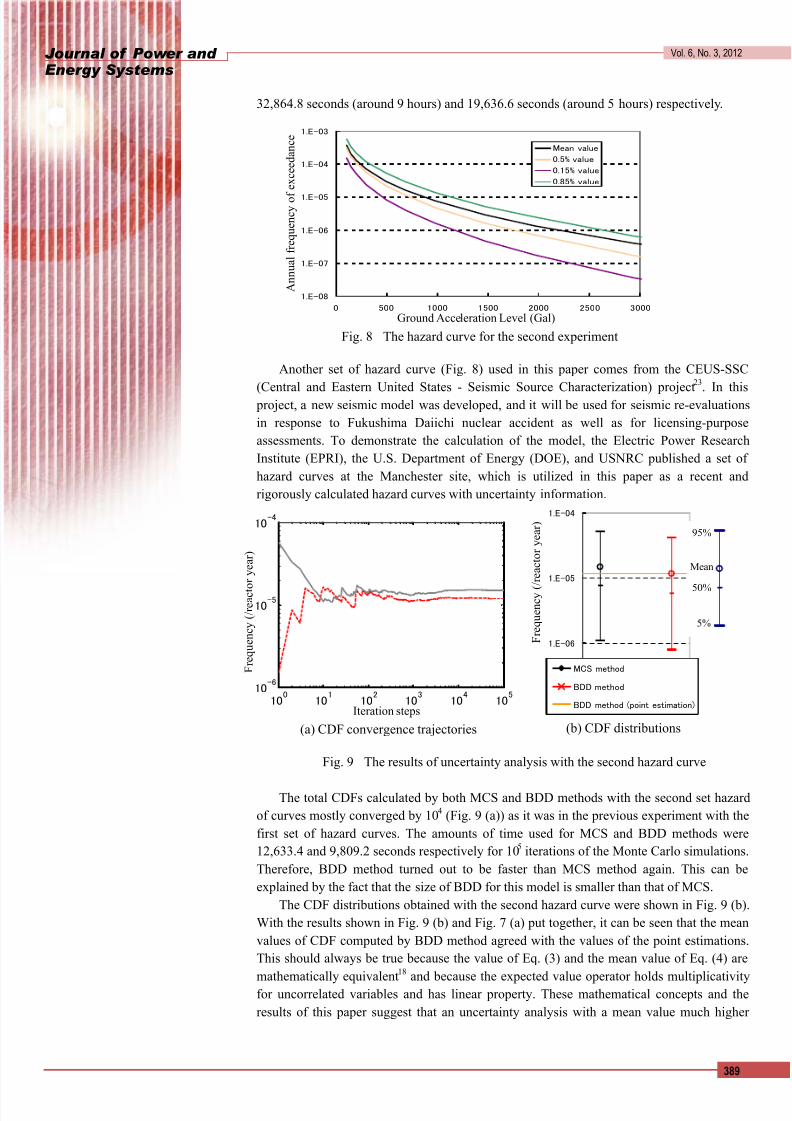
Fig. 9 The results of uncertainty analysis with the second hazard curve

The total CDFs calculated by both MCS and BDD methods with the second set hazard

of curves mostly converged by 104 (Fig. 9 (a)) as it was in the previous experiment with the

first set of hazard curves. The amounts of time used for MCS and BDD methods were

12,633.4 and 9,809.2 seconds respectively for 105 iterations of the Monte Carlo simulations.

Therefore, BDD method turned out to be faster than MCS method again. This can be

explained by the fact that the size of BDD for this model is smaller than that of MCS.

The CDF distributions obtained with the second hazard curve were shown in Fig. 9 (b).

With the results shown in Fig. 9 (b) and Fig. 7 (a) put together, it can be seen that the mean

values of CDF computed by BDD method agreed with the values of the point estimations.

This should always be true because the value of Eq. (3) and the mean value of Eq. (4) are

mathematically equivalent

18

and because the expected value operator holds multiplicativityfor uncorrelated variables and has linear property. These mathematical concepts and the

results of this paper suggest that an uncertainty analysis with a mean value much higher

1.E-08

1.E-07

1.E-06

1.E-05

1.E-04

1.E-03

0 500 1000 1500 2000 2500 3000

Mean value

0.5% value

0.15% value

0.85% value

Fig. 8 The hazard curve for the second experiment

A n n u a l f r e q u e n c y o f

e x c e e d a n c e

Ground Acceleration Level (Gal)

1.E-07

1.E-06

1.E-05

1.E-04

MCS method

BDD method

BDD method (point estimation)100

101

102

103

104

105

10-6

10-5

10-4

95%

Mean

50%

5%

(b) CDF distributions(a) CDF convergence trajectories


Iteration steps

F r e q u e n c y (

/ r e a c t o r y e a r )




Vol. 6, No. 3, 2012

390

than the result of point estimation (such as the result shown in table 7 of Ref. (24)) may not

have yet reached a certain degree of convergence. Indeed, if the simulations are stopped

around 102 iterations in the experiments in this paper, the means of CDFs will be highly

overestimated (Fig. 7 (b) and Fig. 9 (a)).

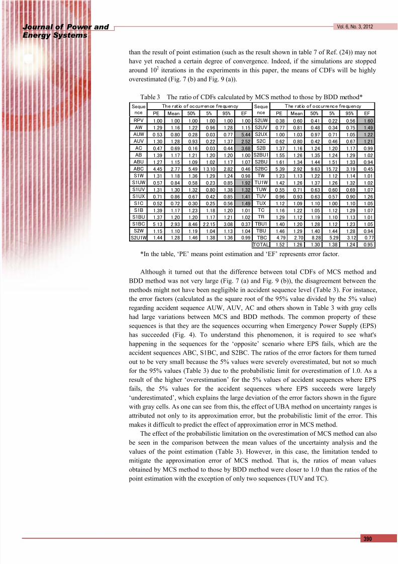
Table 3 The ratio of CDFs calculated by MCS method to those by BDD method*

*In the table, ‘PE’ means point estimation and ‘EF’ represents error factor.

Although it turned out that the difference between total CDFs of MCS method and

BDD method was not very large (Fig. 7 (a) and Fig. 9 (b)), the disagreement between the

methods might not have been negligible in accident sequence level (Table 3). For instance,

the error factors (calculated as the square root of the 95% value divided by the 5% value)

regarding accident sequence AUW, AUV, AC and others shown in Table 3 with gray cells

had large variations between MCS and BDD methods. The common property of these

sequences is that they are the sequences occurring when Emergency Power Supply (EPS)

has succeeded (Fig. 4). To understand this phenomenon, it is required to see what's

happening in the sequences for the ‘opposite’ scenario where EPS fails, which are the

accident sequences ABC, S1BC, and S2BC. The ratios of the error factors for them turned

out to be very small because the 5% values were severely overestimated, but not so much

for the 95% values (Table 3) due to the probabilistic limit for overestimation of 1.0. As a

result of the higher ‘overestimation’ for the 5% values of accident sequences where EPS

fails, the 5% values for the accident sequences where EPS succeeds were largely

‘underestimated’, which explains the large deviation of the error factors shown in the figure

with gray cells. As one can see from this, the effect of UBA method on uncertainty ranges is

attributed not only to its approximation error, but the probabilistic limit of the error. This

makes it difficult to predict the effect of approximation error in MCS method.

The effect of the probabilistic limitation on the overestimation of MCS method can also

be seen in the comparison between the mean values of the uncertainty analysis and the

values of the point estimation (Table 3). However, in this case, the limitation tended to

mitigate the approximation error of MCS method. That is, the ratios of mean values

obtained by MCS method to those by BDD method were closer to 1.0 than the ratios of the

point estimation with the exception of only two sequences (TUV and TC).

PE Mean 50% 5% 95% EF PE Mean 50% 5% 95% EF

RPV 1.00 1.00 1.00 1.00 1.00 1.00 S2UW 0.38 0.60 0.41 0.22 0.56 1.60

AW 1.29 1.16 1.22 0.96 1.28 1.15 S2UV 0.77 0.81 0.48 0.34 0.75 1.49

AUW 0 .53 0.80 0.28 0.03 0.77 5.44 S2UX 1.00 1.03 0.97 0.71 1.05 1.22

AUV 1.30 1.28 0.93 0.22 1.37 2.52 S2C 0.62 0.80 0.42 0.46 0.67 1.21

AC 0.47 0.69 0.16 0.03 0.44 3.68 S2B 1.37 1.16 1.24 1.20 1.17 0.99

AB 1.39 1.17 1.21 1.20 1.20 1.00 S2BU1 1.55 1.26 1.35 1.24 1.29 1.02

ABU 1.27 1.15 1.09 1.02 1.17 1.07 S2BU 1.61 1.34 1.44 1.51 1.33 0.94

ABC 4.45 2.77 5.49 13.10 2.82 0.46 S2BC 5 .39 2.92 9.63 15.72 3.19 0.45

S1W 1.31 1.18 1.36 1.29 1.24 0.98 TW 1.23 1.13 1.22 1.12 1.14 1.01

S1UW 0.57 0.84 0.58 0.23 0.85 1.92 TU1W 1.42 1.26 1.37 1.26 1.32 1.02

S1UV 1.31 1.30 1.32 0.80 1.38 1.32 TUW 0 .55 0.71 0.63 0.60 0.69 1.07

S1UX 0.71 0.86 0.67 0.42 0.85 1.41 TUV 0.96 0.93 0.63 0.57 0.90 1.26S1C 0.52 0.72 0.30 0.25 0.56 1.49 TUX 1.12 1.09 1.10 1.00 1.10 1.05

S1B 1.39 1.17 1.23 1.18 1.20 1.01 TC 1.16 1.22 1.05 1.12 1.29 1.07

S1BU 1.37 1.20 1.20 1.17 1.21 1.02 TB 1.29 1.12 1.19 1.10 1.13 1.01

S1BC 5 .13 2.93 8.46 22.15 3.08 0.37 TBU1 1.40 1.20 1.28 1.12 1.23 1.05

S2W 1.15 1.10 1.19 1.04 1.13 1.04 TBU 1.46 1.29 1.40 1.44 1.28 0.94

S2U1W 1.44 1.28 1.46 1.38 1.36 0.99 TBC 4.79 2.70 8.28 5.29 3.12 0.77

TOTAL 1.52 1.26 1.30 1.38 1.24 0.95

Sequence

Sequence

The ratio of occurrence frequency The ratio of occurrence frequency




Vol. 6, No. 3, 2012

391

4. Conclusions

This paper has examined the accuracy and the computational time of MCS, MC, and

BDD methods in uncertainty analysis as well as in point estimation. As to the accuracy, it

was confirmed that the results calculated by MC method agrees well with that by BDD

method, which is the exact solution, in both point estimation and uncertainty analysis. On

the other hand, it was observed that the approximation error of MCS method in point

estimation can cause CDFs per accident sequence to be inconsistent in the similar degree

with those presented in Ref. (8); while some accident sequences were overestimated, others

were underestimated, and hence the rank of dominant accident sequences can be

misleading. However, the result of this paper has shown that the inconsistency in using the

MCS method abated in the uncertainty analysis since the right tails of overestimated CCDP

distributions are limited by the probabilistic upper bound of 1.0. The more essential reason

as to why MCS method did not agree was that the MCS method needs to use approximation

methods as expressed in Eqs. (3) and (3)’. Therefore, although it is always preferable to use

BDD or MC method in terms of accuracy, MCS method may not be as bad of an option in

the uncertainty analysis as it is in the point estimate calculation.

As for the computational time, uncertainty analyses in this study required at least 104

Monte Carlo iterations to archive a certain degree of convergence for total CDF no matter

which method was used. The comparison of the amounts of time used by the three methods

has shown that the fastest method was BDD method, the second was MCS method, and the

third was MC method. More concretely, while BDD and MCS methods required around 9

hours and 5 hours respectively for 105 iterations, MC method spent around 376 hours to

perform 104 iterations.

Based on the accuracy and the computational time discussed above, BDD method can

be considered as the most effective method. However, BDD method is not always

applicable to a large Fault-tree and Event-tree as discussed in this paper by referring

previous works. Therefore, if BDD method turns out to be inapplicable, or if time is not a

serious concern in a PSA study, MC method is a great alternative to be used for both point

estimation and uncertainty analysis. In fact, the case where computational time is an

extremely huge factor for a PSA study would be almost only when online monitoring of the

risk (Risk Monitor) is involved in the study. Therefore, for seismic PSA without online risk

monitoring, the applicability of MC method would be very high. Though, because MC

method was confirmed to require a lot of time for uncertainty analysis in particular, it may

be a good idea to use MCS method to obtain a rough estimation in uncertainty analysis if

the error properties of the approximation are carefully considered, such as the effect of

probabilistic upper bound on error factors, which was revealed in this paper. Note that

acceptable accuracy and computational time vary for different PSA studies and thereby this

paper cannot identify one perfect method. Instead, this study provides information for

researchers and analysts to select a suitable method in accordance with their acceptable

levels for accuracy and computational time.

The points made in this paper were supported by using only one PSA model. However,

it is clear that the results of this study depend only on the complex structures of Boolean

functions and on the existence of high probabilities for basic events, both of which are

common in seismic PRA models for NPPs. Thus, the qualitative implications of the results

in this paper are likely to be applicable to almost all seismic PRA models for NPPs and even

to other PSA models having such properties. Some major points that are newly reveled in

this study are listed in the following as a brief summary.

- MCS method may underestimate accident sequences as well as overestimate them.

- MC (DQFM) method tends to underestimate risks until the enough number of iterationis conduced (see Section 3.2 for more information as to the concrete number).

- MC method agrees well with exact solutions in uncertainty analysis as well as in point

Efficiency of Analytical Methodologies in Uncertainity Analysis of Seismic Core Damage Frequency

Documents

Transcript of Efficiency of Analytical Methodologies in Uncertainity Analysis of Seismic Core Damage Frequency