Efficiency and Market Structure: Testing for Profit Maximization in African Agriculture

Christopher Udry

Department of EconomicsNorthwestern University

Evanston, IL 60208

udry@nwu.edu

June, 1996

Marcel Fafchamps, Elaina Rose and John Strauss provided valuable comments and advice on anearlier draft. I thank the International Crop Research Institute for the Semi-Arid Tropics and theInternational Food Policy Research Institute for making data available. Ellen Payongayongprovided vital assistance with the IFPRI Kenya data. Financial assistance from the NSF isgratefully acknowledged. The most current version of this paper is available online athttp://www.econ.nwu.edu/faculty/udry/.

1

1. Introduction

A central question in development economics is the extent to which the rural environment

is characterized by competitive markets. The answer has direct implications for the efficiency of

the allocation of resources, for the design of economic policy, and for the choice of appropriate

analytic methods. Hence, an important task of empirical development economics is to provide a

characterization of the market environment in rural areas of poor countries. Much of the relevant

literature has been concerned with the existence of well-behaved labor and land markets (e.g.,

Benjamin, 1992; Collier, 1983; Rosenzweig, 1988; Pitt and Rosenzweig, 1986; Binswanger and

Rosenzweig, 1981), but there has also been extensive interest in intertemporal and insurance

markets (e.g., Morduch, 1990; Chaudhuri, 1993; Deaton, 1991; Carter, 1994; Townsend, 1994).

For historical reasons, the task of an empirical characterization of rural market structure is

furthest advanced in Asia and Latin America. Relatively little is known of the extent or

characteristics of markets in rural Africa. The goal of this paper is to improve this base of

knowledge by using agronomic information to provide evidence on the basic characteristics of

rural markets in a variety of African settings.

An implication of the availability of a complete set of competitive markets that greatly

simplifies empirical work is separation: the household maximizes profit in its production decisions

without regard to its preferences (Krishna, 1964). The null hypothesis of complete markets may

seem incredible and thus unworthy of testing. It is true, of course, that nowhere in rural Africa

(or anywhere else) does there exist an economy characterized by a complete set of competitive

markets. However, a broad variety of spot markets do exist, and in some contexts appear to

operate competitively (e.g., Hays, 1975; Jones, 1980; Pingali et al, 1987). Informal mechanisms

Separation is also invoked, usually without comment or testing, in studies of production in rich countries.1

2

exist which might fill the same functions as other competitive markets (Udry, 1990; Aryeteey,

1993; Guyer, 1981). Moreover, the separation result is robust to the non-existence of some

markets (for example, it is retained if there is no market for one of the factors of production).

The most practical reason for testing the separation hypothesis, however, is that separation is

commonly invoked in empirical studies of agricultural production in poor countries (Singh et al,

1986). 1

The separation theorem, therefore, serves as a simple and useful benchmark for further

analysis. In addition, much can be learned from rejections of the exclusion restrictions that are

implied by separation. The pattern of rejections has implications for the structure of rural

markets. This pattern, and its variation over space, can provide useful information about the

geography of markets.

The empirical work of this paper consists of a series of tests of separation in a variety of

African contexts. The African setting is of interest because the quantitative literature on rural

factor markets in Africa remains quite limited, and that which does exist contains arresting

suggestions of empirical regularities which look quite different from other parts of the world. The

most important example concerns a “stylized fact” of traditional agriculture (Bardhan, 1973): the

inverse relationship between farm size and yield. This pattern has been established in a variety of

data sets from Asia and Latin America. The limited evidence from Africa, however, looks

different. Hill in west Africa and Kevane (1994) in Sudan both show (using small data sets) the

opposite relationship - larger farms have higher yields than smaller farms. In contrast, Barrett

(1996), Gavian and Fafchamps (1995) and Collier (1983) find that in Madagascar, Niger and

3

Kenya, respectively, there is evidence of the conventional inverse relationship.

Section 2 describes the separation result, and discusses the exclusion restrictions which it

implies. It also raises the most important econometric issue which arises in this context - the

possibility that apparent violations of separation are the result of unobserved variation in farm

characteristics. Section 3 presents the data from a wide variety of sources which are used to

implement the tests. The results are presented, country by country, in section 4.

2. Separation and Profit Maximization

A. A Review of the Separation Result and its Relation to Profit Maximization.

Consider a household with a conventional utility function over vectors of goods (c ) andst

leisures (l ) in state s S of period t T (so c is the vector of goods consumed if state s occurs inst st

period t). For simplicity, assume that both S and T contain finite numbers of elements. This

household faces a complete set of competitive markets. Let p and w be the price vectors of thest st

state-contingent goods and labor. Let E be the household's endowment of time in state s andst

period t, q be the price of farm output, L be the labor used on the household’s farm, A be thest st st

vector of land inputs and r is the vector of prices of these land inputs (to simplify notation, I havest

assumed that there are no inputs other than land and labor - these can be accommodated with no

substantive change in the analysis). F (L ,A ) is a set of (state-contingent) production functions. st st st

Then the household's problem is to

(1) Maxcst,lst,Lst

U(cst,lst) subject to

(2)t T, s S

wst Est st pst cst wst lst 0,

(3) st qst Fst(Lst, Ast) wstLst rstAst, Lst, Ast 0 and(4) cst , lst 0, lst Est.

(5) Maxcst,lst

U(cst,lst) subject to

(6)t T, s S

wst Est st(qst, wst, rst) pstcst wst lst 0, and

(7) cst , lst 0, lst Est,

(8) st(qst, wst, rst) MaxLst, Ast

qst Fst(Lst, Ast) wstLst rstAst, Lst, Ast 0.

Note that the choice of the household as the unit of analysis has no effect on this particular result. If markets are2

complete, separation holds for all standard models of the household - the cooperative bargaining models, the collectivemodel, and even for most non-cooperative models of the household.

It should be noted that (8) does not describe expected profit maximization. Profits are maximized separately in each3

state of nature. It is unrealistic, of course, to presume that households can adjust labor and land inputs in each state ofnature, because some inputs must be committed before the state is realized. To examine the consequences of this fact oflife, suppose that in each period t, labor (L ) and land (A ) are chosen before the state of nature for that period is realized. t t

4

The problem is recursive. With weak conditions on U(.), (2) is binding at the solution and

the maximized value of U(.) is increasing in . L and A appear only in (3). Hence (1) - (4)st st st

can be solved by first maximizing profit with respect to L and A and then maximizing utility. st st st

That is, the problem (1) - (4) is equivalent to:

where

Households maximize profits in each state and on each date and, therefore, production decisions

on any plot, depend only on prices and the characteristics of that plot. The simplification is2

extraordinary: from a problem (1-4) of dealing with a (risk averse) household's dynamic behavior

in a risky environment we arrive at a very simple static profit-maximization problem. 3

(8 ) t MaxLt ,At s

qst Fst(Lt ,At) wtLt rtAt.

(2 )t

[wt Et t wtlts

pstcst ] 0

(3 ) ts

qstFst(Lt,At) wtLt rtAt

Factor prices, therefore, are no longer state-contingent. The budget constraints (2) and (3) now become:

The problem remains recursive, and (8) becomes

Production decisions remain a function only of prices and the characteristics of the plot.

5

Equation (8) provides the basis of the empirical strategy of the paper. Within any group

of plots subject to the same prices, input choices (and outputs) are identical on identical plots.

This paper present two series of empirical tests based on this restriction. The first examines the

distribution of yields and inputs on similar plots. Since separation implies that output and inputs

are identical on identical plots, we examine the dispersion of yields and input intensities on

apparently identical plots. Is this dispersion so large that the null hypothesis of separation must be

rejected?

The second series of tests is based on the strong exclusion restrictions on input demand

and output supply functions which are implied by (8): input demand and output supply functions

depend on prices and on plot characteristics but nothing else. Controlling for prices and plot

characteristics, is there a strong enough correlation between input use (or output) and other

household characteristics that we must reject the null hypothesis of complete markets?

Now consider production on a particular plot i. From (8), yield (output per unit area) on

(9) Q i G(A i,w,r,q).

(10) Q i Q G(A)/ A [A i A ] i K,

(10 ) ln(Q i) ln(Q) (v 1)v

[ln(A i) ln(A)].

A i Q i [ (A i) (1 )(L i) ]v

,

6

that plot (in state s of period t, but I drop those subscripts to simplify notation) depends only on

prices and the characteristics of the plot itself:

Consider a set of plots K, each of which is subject to the same prices (w, r, and q). Then a first

order Taylor expansion of (9) across plots i K implies

where A is the mean area of the plots planted with the same crop and subject to the same prices.

Within groups of plots subject to the same prices (in this paper, I will assume that plots in a

particular village face the same prices), the deviation of yield on a plot from the group average

yield is a function only of the deviation of the plot's area from the average area of plots in the

group. With a flexible specification for the function G(A)/ A, (10) is an approximation to an

arbitrary concave production function. If one assumes that the technology is CES, so that

then (10) becomes

The first evidence that I examine is extent to which agricultural data from Africa matches

the theoretical prediction that yield is identical on identical plots. This evidence is summarized by

estimates of the distribution of deviations of actual yield from expected yield. The second type of

evidence is drawn from tests of the exclusion restrictions implied by (10): if markets are complete,

then yield depends only on prices and plot characteristics, not on other characteristics of the

(11) Qvhtci Qvtc G(X, ) / X [Xvhtci Xvtc ] G(X, ) / [ vhtic¯

vtc ].

Crop choice, as well as input choice conditional on crop, depends only on prices and plot characteristics if markets4

are complete. Tests based on this fact would provide another avenue through which agronomic information could beused to test the separation hypothesis.

7

household which cultivates the plot.4

B. The Empirical Strategy.

Much of the empirical work of this paper is based on a series of tests of the exclusion

restrictions implied by (10) and (10'). Each of the tests has power against different violations of

the assumptions which imply separation. The pattern of violations, therefore, can provide

information about the structure of rural markets. It is to be expected that the pattern of violations

will vary across areas.

Some issues remain before (10) or (10') can be estimated. Contrary to (10) and (10'), of

course, A is not scalar-valued. Plot i has characteristics in many dimensions - its area, its soili

quality, its topography, the particular amount of rain it receives in state s. Moving to a notation

more amenable to a discussion of econometric specification, let A be composed of twoi

components: X , which is a vector summarizing the information about plot i (planted to crop cvhtci

in year t by household h in village v) available to the researcher and , a set of unobservedvhtci

characteristics of the plot (including plot level random shocks as well as more permanent

unobserved characteristics), so G(A) G(X, ). Prices are assumed to be the same for all plots in

the same village v in a particular year t. Equation (10) becomes:

is unobserved, so the final part of the expression is subsumed in an error term (about which

more will be said) and I approximate G()/ X with a linear function:

(12)Qvhtci Qvtc [ Xvhtci Xvtc] vhtci ¯vtc

Xvhtci vtc vhtci .

(13)(a) Qvhtci Xvhtci vtc

vvhtci

(b) Qvhtci Xvhtci vhtchvhtci .

Model specification choices must be made to characterize G()/ X. The econometric work is cast in per-hectare5

terms, with log yield and log input intensity as dependant variables. I estimate G()/ X×X as X , where X includes logplot area and dummy variables characterizing the plot's topography, location and soil type. In this specification, thecoefficient on, say, a dummy variable representing a soil type can be interpreted as the percentage increase in the yield ofa plot of that soil type over the base soil type. There is concern about heteroskedasticity and the standard errors areappropriately adjusted.

8

(12) is the basic empirical framework of the paper. 5

It is now possible to define the two series of empirical tests of the paper. First, is output

identical on identical plots? This is a question about the characteristics of . If the null

hypothesis of complete markets is correct, then the distribution of is determined by the

distribution of . Is there a sense in which we can say that in a particular sample, the distribution

of estimated residuals is not compatible with the null hypothesis? Such tests can be performed if

relatively strong assumptions about are valid. Second, (8) implies a series of very strong

exclusion restrictions in (12). In particular, input demand and output supply depend on prices and

plot characteristics and nothing else. Other household characteristics such as farm size, household

composition or wealth have no role in (12).

The first series of tests is based on the maintained assumption that the allocation of factors

of production across the various plots controlled by an individual is efficient, so that the

separation hypothesis is true across these plots. Consider the following pair of regressions:

(14) Qvhtci Xvhtci Evhtci vtc vhtci,

The most recent paper in this tradition is Barrett (1996).6

9

(13a) is identical to (12), while (13b) replaces the village-year-crop fixed effect with a household-

year-crop fixed effect. Attention is restricted to one farmer in each household, so the distribution

of reflects the variation in yields across apparently identical plots cultivated by a singleh

individual. The distribution of , therefore, is a function of the distribution of across plotsh

controlled by an individual. Now consider , the error term defined in (13a). If the distributionv

of across plots within a household-year-crop group is the same across plots within a village-

year-crop group, then if separation is valid, the distribution of should be the same as that of . v h

The first series of tests, therefore, is based on a comparison of the distributions of and .v h

The second line of questions is based on the exclusion restrictions implied by (8). (8)

implies that =0 in the regression

where E is the exclusion restriction under consideration. I consider tests based on three sortsvhtci

of exclusion restrictions: farm size, household demographics, and wealth or cash flow.

The first exclusion restriction is that the total area cultivated by the household should have

no effect on output on a particular plot if the null hypothesis is correct. This test is closely related

to the large literature which finds an inverse relationship between farm size and yield, or farm size

and labor demand. If agricultural production is governed by a CES technology with constant6

returns to scale, then the log of farm area should have a coefficient of zero in a regression of the

log of yield on the log of farm area (see equation (10'), v=1 is the case of constant returns to

scale). In fact, it is often found that the coefficient of farm area is negative. The earliest and most

popular explanation for this regularity is market failure of some sort - small and large farms face

10

different opportunity costs and hence optimally choose different mixes of inputs on their farms.

This type of explanation is sensible and probably correct in many instances, but the connection

between the result and the conclusion is not direct. Bhalla (1988) and Benjamin (1991) argue that

unobserved variations in land quality could underlie the oft-observed inverse relationship between

farm size and yield - larger farms are less fertile, and thus are optimally farmed less intensively.

The analysis in this paper is conducted at the plot level, as specified in (12), with E defined asvhtci

the area cultivated by the household on plots other than plot i. I show below that this mitigates

the problem of measurement error.

The second series of tests is based on household demographic measures. This is a

standard test of the assumptions which imply separation. Do larger households (controlling for

land area) farm more intensively? Benjamin (1992), Kevane (1994) and Pitt and Rosenzweig

(1986) are key recent papers. The third set of tests is concerned with correlations between input

demand and non-farm wealth, income and cash flow (Swamy, 1993; Chaudhuri, 1993; Morduch,

1990; Rosenzweig and Binswanger, 1993).

i. Unobserved Plot Quality Variation and Type I Error.

Each of these tests, however, is subject to a similar important econometric caveat. Under

separation, cropping decisions depend only on prices and plot characteristics. I can account for

prices through village fixed effects provided that the model is linear. Plot characteristics,

however, are problematic. There is undoubtedly unobserved variation in land quality. Therefore,

there is a classic omitted variables problem and the bias induced by this problem could lead us to

reject the null hypothesis of separation when separation is in fact true.

Consider the relationship between farm size and output. Suppose that in fact F(.) exhibits

(8 ) MaxAvhi 0

qF(Lvh, Avhi(1 vhi )) r( vhi ) Avhi ,

A Avhi

(1 vhi)< 0

11

constant returns to scale and that separation is true. Suppose, however, that there are unobserved

(to the analyst) plot characteristics (soil type, weather shocks, etc...), so that Q = F(L ,T ),vhi vhi vhi

where T = A (1+ ), A is observed plot area and is an unobserved land-augmentingvhi vhi vhi vhi vhi

plot characteristic (dropping tc subscripts to shorten the notation). A regression of output on T

would yield an estimated coefficient of one, given the validity of the separation hypothesis.

However, the regression of output on plot area is subject to omitted variables bias because isvhi

not included in the regression. The sign and size of that bias depends on the covariance of A and

. If the unobserved variation in land quality is uncorrelated with the area of the plot then the

regression is subject to attenuation bias and we will find a less than proportional relationship

between output and plot area.

Worse, there is reason to expect that unobserved land quality is worse on larger plots than

on smaller plots. Suppose, for example, that all markets exist and operate smoothly except the

labor market. If each household has access to one type of land ( ) and cultivates only one plot,vhi

then in each state of each period, each household's production problem is to solve:

where L is the amount of labor time the household chooses to spend working. Choose units sovh

that for some plot k, =0. Then define r = r( ). Competition in the land market ensures thatk k

r =r (1+ ). By the implicit function theorem, . Hence plot quality willvhi vhi

be negatively correlated with plot size in the cross-section. A regression of yield on T would

(8 ) MaxAvhi,Lvhi 0 i P

F(Lvhi, Avhi(1 vhi )) r (1 vhi ) Avhi

s.t.i P

Lvhi Evh

i P( Avhi vhi)

Evh

Blarel et al. conduct a similar exercise, but don't examine the implications for separation. 7

12

produce an estimated coefficient of 0. The omission of land quality from the regression of yield

on land area, however, will bias the estimated coefficient on land area down from zero because of

the negative correlation between unobserved land quality and land area.

It is also true, of course, that if F() has DRTS (v < 1 in (10')) then there will be a direct

technological explanation for the inverse relationship. In order to eliminate the technological

possibility and to attenuate the problem of unobserved land quality, I propose to estimate (14)

with E equal to the area of other household plots. Are plots of a given size cultivatedvhtci7

differently depending upon the total area on other plots that are cultivated by the same household?

It is clear that this specification eliminates the potential technological explanation for the

inverse relationship. It also mitigates, but does not eliminate, the problem of omitted variables

bias due to unobserved variation in plot quality. Under the null hypothesis of separation, we

expect in (14) to be zero. Any attenuation bias due to unobserved variation in land quality that

is uncorrelated with farm area, therefore, cannot cause a false rejection of the null. However,

there is still reason to expect an inverse correlation between the quality of a given plot and the

area cultivated by the household on other plots. To see why, consider the household's problem

when it cultivates many plots of different qualities:

If F() is constant returns to scale, (8''') implies that is a constant which depends

13

only on r. Hence if for a plot i, is particularly low, then the household optimally farms thatvhi

land with relatively low intensity. At the same time (given E and r), the household optimally

acquires more land, either on plot i or on other plots. If some of the land acquired is on other

plots, there will be a negative correlation between the quality of plot i and the area cultivated by

the household on other plots. We would then estimate <0 even if separation is valid.

The tests of exclusion restrictions with respect to demographic variables are also subject

to misinterpretation as a consequence of unobserved variation in plot quality. Suppose again that

labor markets do not work well, but that land rental markets remain perfect, so that separation

still holds. It remains the case that under constant returns to scale the ratio of quality adjusted

land holdings to household labor availability is a constant. If households can choose the quality of

the land that they cultivate (by choosing which plots to cultivate), then household size will be

positively correlated with unobserved land quality. Unobserved land quality is also a potential

cause of misinterpretation of tests of exclusion restrictions with respect to cash flow or wealth.

Unobserved good quality land can be associated with high income, wealth and cash flow, hence

potentially causing to appear positive even if separation is true.

There are a variety of avenues for exploring the potential importance of unobserved

variation in plot quality beyond the strategy of attenuating the bias by using plot level information.

a. The natural solution, of course, is to use IV estimates. Unfortunately, while there are

plenty of variables that are correlated with farm size, plot size, household demographics and non-

farm income, it is very difficult to make the case that any of these are uncorrelated with

unobserved land quality. I have not, therefore, been able to identify likely instruments in any of

the available datasets.

14

b. Unobserved land quality variation is less of an issue in one of the data sets used in this

paper than in most data from developing countries. The ICRISAT Burkina Faso data contains

rich information on plot characteristics. For the other data, the use of village-crop-year fixed

effects, as well as some plot-specific information, permits a finer degree of control for land quality

than has been possible in most previous investigations of related issues (Benjamin, 1992, 1994).

In addition, some diagnostic lessons may be drawn from the exercise of conducting tests of the

exclusion restrictions with and without a subset of the plot characteristics data. If unobserved

land quality is positively correlated with observed land quality, and if inclusion of observed

measures of land quality reduces the effect of the test variables, this heightens our concern that

unobserved land quality may be causing false rejections of the null of separation.

c. It is possible (though difficult) to trace plots over time in some of these data. This is

implemented in the Kenya data set discussed below. Plot fixed effects, then, can control for

unobserved land quality. Many observations are lost due to the difficulty of matching plots, and

there is heightened concern regarding measurement error in the variables tested for exclusion

(Ashenfelter et al), but the additional confidence gained with respect to land quality is valuable.

ii. What Causes Rejections of Separation?

Suppose that it is found that output on one plot controlled by a household decreases with

the amount of land on other plots cultivated by the household, and increases in the size of the

household, and that it is concluded that these correlations are not attributable to specification

error. It would seem that the implication is that both labor and land markets in the economy

under investigation are imperfect, thus preventing households from realizing the gains which are

potentially available from trading land or labor to equalize marginal products across plots

(13)Max

c1,c2, l,L fU(c1, l) (1 )U(c2, l)

s.t. p1c1 p2c2 wl (p1 1 p2 2) f(L f) wL f wE

(14)Maxc1,c2,l

U(c1, l) (1 )U(c2, l)

s.t. p1c1 p2c2 (p1 1 p2 2) f(E l).

Benjamin (1992) provides a thorough discussion of the power of a similar test to detect specific violations of the8

assumption of perfect labor markets when E contains demographic variables. He examines the specific alternativehypotheses that there is a binding constrain on obtaining off-farm employment, a binding constraint on hiring labor, andthe more general possibility that the returns to on- and off-farm labor differ. Bardhan (book) offers a similar treatment ofthe power of the test when E contains farm size.

15

controlled by different households. It is true, in fact, that (14) can detect violations of the

assumption of perfect labor and/or land markets. However, Srinivasan (1972) (and more recently8

Feder, 1985; Eswaran and Kotwal, 1986; Carter and Wiebe, 1990; Banerjee and Newman, 1993;

Barrett, 1996) show that violations of the assumption of complete insurance or intertemporal

markets can also cause rejections of the exclusion restrictions with respect to household

demographics or the area of other plots.

To examine the import of this ambiguity, consider the simplest model in which it can arise.

There are two states of nature (the probability of state 1 is ) with multiplicative production risk

( ). A household with fixed land and labor endowments makes production and labor-leisurei

decisions before the resolution of output uncertainty. With complete labor and insurance markets,

(but no land market) the household’s problem is to:

where L is the amount of labor used on the farm, and E is the household’s labor endowment. f

Separation holds, and the household maximizes profit on the farm. In contrast, if there are

complete insurance markets, but no labor market, then the household solves:

dL f

dL

U 1ll (1 )U 2

ll

U 1ll (1 )U 2

ll fLL

(15)

Maxc1,c2, l,L f

U(c1, l) (1 )U(c2, l)

s.t. p1c1 wl p1 1 f(L f) wL f wEp2c2 wl p2 2 f(L f) wL f wE.

(16) 0 1( 1p1 f (L f) w) 2( 2p2 f (L f) w)

To be more precise, if derivatives are denoted by subscripts, is the lagrange multiplier, and U =0, then 9cl

which is positive and less than one.

16

This is analogous to Sen’s (1966) formulation of an autarkic farm household under certainty and

separation is violated. Farm output increases in the household's labor endowment.9

Finally, if the labor market is complete, but there is no insurance the household solves:

The first order conditions of this problem include

where is the marginal utility of income in state i. Separation does not hold because inputi

decisions depend on the ratio of the marginal utility of income in the two states. An increase in

the household’s endowment of labor will affect this ratio (increasing relative to if > 1 2 1 2

and the household has diminishing absolute risk aversion) and thus change input decisions.

The violation of separation along a particular dimension - in this instance the correlation

between household demographics and production - is not conclusive evidence of a particular

market failure. However, we can examine the separation hypothesis along various dimensions (in

this paper, effects of household demographics, farm size, and non-farm income). Particular

configurations of results that are revealed by this series of tests can provide evidence of particular

See Matlon (1988) for documentation of the survey.10

4787 plots were cultivated by the sample households over the three years; 132 of these plots did not have their area11

measured and so were dropped from the sample. 2079 plots were excluded because they were cultivated by peopleother than household heads, thus raising complex issues of intrahousehold resource allocation.

17

market failures. A complete taxonomy is possible, but it would be lengthy. Instead, I provide this

analysis in the discussion of the results of the case studies in Kenya and Burkina Faso (section 4).

3. Data

A. Burkina Faso

The data used for this study are drawn from the Burkina Faso farm household

survey conducted by the International Crops Research Institute for the Semi-Arid Tropics

(ICRISAT). The survey was a four year panel study (1981-1985) of 150 households in six10

villages in three different agro-climatic zones of Burkina Faso. This study uses data from the first

three agricultural seasons of the survey (1981-83), during which the most detailed agronomic

information was collected. During these three seasons, enumerators visited the sample

households approximately every 10 days to collect information on farm operations, inputs and

outputs on each of the household's plots since the previous visit. These three seasons of data

collection result in 432 household-years of data on agricultural activities, with usable data on a

total of 2576 plots cultivated by household heads. An important advantage of these data for this11

study is the fact that they contain rich descriptive information concerning the area (measured by

the enumerators), topography, location and soil characteristics of the plots cultivated by the

households.

All of the farmers in the survey are poor, with an average income per capita of less than

18

$100 (Fafchamps, 1993). The farming system is characteristic of rainfed agriculture in semi-arid

Africa: each household simultaneously cultivates multiple plots (10 is the median number of plots

per household in any year) and many different crops (a median of 6 different primary crops on the

plots farmed by a household in a given year).

B. Kenya

The Kenya data are drawn from a 1985/87 survey of 617 households conducted by IFPRI

in South Nyanza, a sugar-growing area of Kenya (see Cogill, 1987 for a description of the

survey). Data from two rounds of this survey, covering successive cropping seasons, is used.

There is usable data on output on 3194 cultivated plots over these two seasons. These data do

not contain as rich information on plot characteristics as do the data from Burkina Faso, but they

do have an important advantage. Many of the plots can be traced over the two seasons,

permitting the use of fixed effect estimators to mitigate the problem of unobserved plot

characteristics. As in Burkina Faso, the Kenyan households are poor, with an income per-capita

of about $120 (Kennedy, 1989). Households farm multiple plots (an average of 6 plots per

household) and many crops (about 8 different crops), though maize is the dominant crop,

accounting for between 15 and 30 percent of all farm area, depending on the season (Cogill,

1987). Summary data from both data sets is provided in Table 1.

4. Testing for Profit Maximization

A. Burkina Faso

We begin by examining the characteristics of and in the two regressions (13a) andv h

(13b). X includes the rich set of plot descriptors discussed in section 3A, and and arevhtci vtc vhtc

Equivalently, the F(1684,706) test statistic of the hypothesis that = has a value of 1.429 (p=0.00).12vhtc vtc

19

village-year-crop and household-year-crop fixed effects. The sample is limited to plots cultivated

by household heads (rather than all plots within households) because of the evidence presented in

Udry (1996) that separation is violated across plots controlled by different individuals within

households. I maintain the hypothesis the household head is free to rearrange resources across

the plots he controls as an individual, so separation is a maintained hypothesis in (13b). ,h

therefore, is zero in the absence of measurement error in Q, unobserved variation in plot quality,

and plot-specific risk (which can be considered a form of unobserved variation in plot quality). In

fact, measurement error exists and is not zero: Figure 1 reports a kernel estimate of itsh

distribution. Figure 2 reports the analogous distribution for plot-specific labor demand.

Consider the joint null hypothesis that: (1) separation holds within the village; and (2) the

distribution of measurement error in Q and unobserved variation in plot quality is the same across

households as it is across plots controlled by an individual household head. Under this null, the

distribution of is the same as that of . However, the estimates indicate that has a muchv h v

more diffuse distribution. There is much more variation in both yield and labor demand per12

hectare across similar plots controlled by different households within a village than there is across

plots controlled by a single individual. Some of this additional variation may be a consequence of

greater unobserved plot quality variation across plots controlled by different households than

across plots within a household. The force of this plausible explanation is reduced, however, by

recognition of the fact that plots controlled by individual household heads are dispersed

throughout the village land, probably as one element in an effort to diversify risk. The much

larger dispersion of than raises the possibility that the separation hypothesis is violated.v h

20

Further evidence that separation is violated is provided by the correlations between plot

yield or input intensity and a series of variables which should be orthogonal to yield and input

intensity (conditional, of course on plot characteristics and prices). Table 2, column 1 reports the

results of estimating (14) with E equal to the log of household size. In apparent violation of vhtci

profit maximization, plot yield is increasing in household size, conditional on prices and all

observed characteristics of the plot. The elasticity is about .2 and is significantly different from

zero at any conventional significance level. It is necessary to interpret these results cautiously

because, as noted in section 2B, they could be an artifact of a correlation between unobserved

plot quality and household size. Turn now to an examination of the relationship between plot yield

and the area cultivated by the household on other plots. Again in apparent violation of the

separation hypothesis, column 2 of Table 2 reports a highly significant correlation between plot

yield and the area cultivated by the household on other plots. In this instance, however, plot yield

increases with the area cultivated on other plots. This is a striking result, because the implication

of conventional land and labor market imperfections would have been a negative correlation

between farm size and plot yield; similarly (as shown in section 2Bi) unobserved variation in plot

quality would be expected to lead to a negative correlation between farm size and plot yield. This

result provides further evidence of violations of the separation hypothesis in Burkina Faso, but

broadens the range of potential market failures which should be considered: households with

larger farms cultivate their land more intensively than other households, raising the possibility of

imperfections in credit or insurance markets.

Following Chaudhuri (1993), I explore the possibility of credit constraints by calculating

the correlation between yield (or input intensity) and short-run measures of cash flow. It is

21

possible to use the ICRISAT data to calculate income from non-farm activities and gifts for the

four month preceding clearing activities for the single annual crop season. Estimates of (14) with

E equal to the log of these resource inflows are reported in Table 2, column 3 (the results arevhtci

very similar when non-farm income and gifts are entered separately). Similar plots within village-

crop-year groups of plots are cultivated more intensively by households which receive higher

short-term resource inflows.

There is a positive correlation between plot yield and household size, area cultivated by

the household on other plots, and short term resource inflows conditional on all observable plot

characteristics. The results presented in Table 2, column 4, however, indicate that conditional on

short-term resource inflows and household size (and plot characteristics), plot yield does not vary

with the area cultivated on other plots. On the other hand, plot yield is higher for large

households with large short-term inflows of non farm resources, conditional on other household

characteristics.

Despite the rich information available in this data set regarding plot characteristics,

measurement error induced by unobserved variation in plot quality remains a concern. One

possible interpretation of the results revealed in Columns 1-4 of Table 2 is that there are certain

wealthy households which cultivate large amounts of land, receive a great deal of nonfarm

income, and have many members, and that these households also control land of particularly high

(unobserved) quality. The panel nature of the data permits us to mitigate this concern by

controlling for the average (over time) quality of each household's land. Column 5 of Table 2,

therefore, reports the results of estimating (12) with household fixed effects as well as the village-

year-crop fixed effect. The results change in a manner consistent with the interpretation above.

Maxc1, l1, c2

U(c1, l1, c2)

s.t. p1 c1 p2 c2 q2 F(E l1, T ) G,

Consider the simplest model of a labor market imperfection with smoothly operating credit markets. Production13

takes time, so labor and land are used in period 1 to produce output in period 2. Consumption of goods occurs in bothperiods, and there is an inflow of nonfarm resources (G) in period 1. The price vector of the consumption bundle inperiod t is p and the output price is q . The household has E units of labor, and T of land. The household solvest 2

(suppressing the standard non-negativity constraints):

which has a first order condition of U = q F , where is the lagrange multiplier and / G<0. Hence l / G>0 andl 2 l 1

yield falls with nonfarm resources.

22

Conditional on the household effect, increases in the area cultivated on other plots are now

associated with declines in yield on a given plot. The elasticity is large and statistically significant.

Increases in inflows of nonfarm resources remain associated with increases in plot yield - the

elasticity is .1 and statistically significant. Changes in household size have no perceptible

relationship to plot yield, which may be a consequence of the relative stability of household size

over the three years.

Interpretation:

This pattern of results: a negative correlation between yield and the area cultivated on

other plots and a positive correlation between yield and short-term inflows of nonfarm resources

and (possibly) between yield and household size have strong implications for the structure of rural

markets. First, simple labor and land market imperfections would not lead to this pattern of

results. If the only market failure is that labor and land cannot be traded, than an increase in

nonfarm resources would be associated with an increase in leisure and hence a reduction in yield. 13

However, a combination of financial market and land market failures leads directly to the pattern

of correlations observed in the data. Suppose that the labor market operates freely, but that there

is a binding cash-in-advance constraint on production in the first period. Increases in nonfarm

p1 c1 w1 (L f (E l1 )) Gp2 c2 q2 F(L f ,T )

The utility function is the same as in the previous footnote. The budget constraints now must be met period-by-14

period:

where L is labor demand on the household's farm. The first order conditions include / w = q F/ L , where isf f1 2 1 2 t

the lagrange multiplier on the period t budget constraint and ( / )/ G < 0. Hence we have L / G = w L / L > 0. 1 2 1f f

With F() CRTS, after some algebra one can show 0< L / T<1, hence yield declines with larger farm size.f

23

resource inflows or household size relax this constraint and permit yields to rise, while an increase

in area cultivated on other plots dilutes available inputs and lowers yields. The observed pattern14

of empirical results, therefore, is consistent with imperfections in the financial and land markets,

rather than with labor market imperfections.

Turning to data on farm inputs, Table 3 reports estimated demand functions for the two

most important farm inputs. Columns 1 and 2 estimate the determinants of log plot labor demand

per hectare. In column 1, household effects are omitted and a strong positive correlation is found

between plot labor demand and household size, while plot labor demand declines as the area

cultivated on other plots increases. When household effects are added to the model, the

correlation between household size and plot labor use disappears, but plot labor demand remains

strongly decreasing in the area cultivated by the household on other plots. Column 3 reports

estimates of the determinants of plot manure demand per hectare. Manure use on a particular plot

declines with increases in the area cultivated by the household on other plots. There is no

observable effect of inflows of nonfarm resources on either labor or manure demand, despite the

strong correlation between such inflows and plot yield. A plausible interpretation of this contrast

is that inflows of nonfarm resources affect the timing rather than the level of input application.

There is strong evidence of violations of profit maximization in Burkina Faso associated in

24

particular with changes in the area cultivated by a household on other plots, and with inflows of

non-farming resources. Increases in the inflow of resources not directly tied to cultivation are

associated with more intensive cultivation, and increases in total farm size are associated with

declines in the intensity of cultivation on particular plots. The finding with respect to nonfarm

resources complements the work of Savadogo, Reardon and Pietola (1994) and Reardon,

Crawford and Kelley (1994), who find in Burkina Faso that households with higher nonfarm

income (averaged over a period of years) are more likely to use intensive methods of cultivation

(e.g., animal traction). The pattern is strikingly reminiscent of Polly Hill’s (1982) argument that

poor farming households in the savannah of northern Nigeria are “too poor to farm”. She argues

that a “householder who has an empty granary at the beginning of the farming season may well

have to earn his living every day by means of sundry paid occupations, including farm-labouring,

so that he has no time to cultivate on his own account ... [T]here are many other circumstances in

which it ['too poor to farm'] applies, such as when manure is lacking” (pp. 69-70).

These results provide some evidence concerning the source of the market failure.

Standard models of labor market imperfections obviously could underlie the inverse correlation

between farm size and the intensity of cultivation of plots. The same imperfections, however,

would induce a negative correlation between inflows of nonfarm resources and cultivation

intensity rather than the positive correlation which is observed in the data. An increased inflow of

nonfarm resources would relax the household's budget constraint, inducing the household to

consume more leisure and thus (with imperfect labor markets) to use less labor on their plots.

In contrast, capital market imperfections could cause both of the correlations observed in

the data. With liquidity constraints, an increase in the availability of nonfarm resources permits

25

the household to cultivate more intensively, and an increase in the size of the farm cultivated by

the household further dilutes available resources and reduces the intensity of cultivation of a given

plot. These results suggest, therefore, that further research on market imperfections in Burkina

Faso begin with an examination of financial markets.

B. Kenya

The analysis begins with an examination of the residuals in the regressions (13a) and

(13b). In this instance, X includes a much less rich set of plot characteristics. I maintain thevhtci

hypothesis that the household is free to allocate factors of production efficiently across its various

plots, hence would be zero in the absence of measurement error in plot quality or yield. Figureh

3 reports the distribution of and the corresponding distribution of .h v

Yield is much more dispersed across similar plots cultivated by different households than it

is across similar plots cultivated by a single household (the F(1549,128) test statistic of the

hypothesis that = has a value of 1.836 (p=0.00)). As was the case in Burkina Faso, thehtc tc

much larger dispersion of raises the possibility that the separation hypothesis is violated at thev

village level. However, given the limited information available about plot characteristics, there is

particular reason to be concerned that these results are contaminated by measurement error. The

estimates of from (13a) and (13b) are presented in columns 1 and 2 of Table 4. If there were no

unobserved variations in plot quality, and the production function were CES with CRTS, than the

coefficient of the log of plot area would be zero. The fact that this coefficient is so negative is

striking, and it is difficult to believe that agricultural production is characterized by such strongly

decreasing returns to scale. An inverse correlation between plot size and quality could account

for this result. More importantly, the large decline in the coefficient on plot size when moving

26

from the household-crop-season fixed effects to the crop-season fixed effects specification can be

interpreted as evidence that the dispersion of these unobserved plot characteristics is larger across

plots in the region than it is across plots controlled by individual households. This casts doubt on

the interpretation of the larger spread of than as an indicator of non-separation.v h

It is reasonable, therefore, to treat the tests of exclusion restrictions presented in Table 5

with caution. Column 1 presents the results of the regression testing the exclusion restriction with

respect to household size. Plot output is strongly increasing in household size and the coefficient

is statistically significant at any conventional level. One interpretation of this result is that with

imperfect labor markets, larger households farm their plots more intensively, but other market

imperfections and measurement error correlated with household size should also be considered.

Column 2 of Table 5 shows that plot output is also increasing with the amount of land cultivated

by the household on other plots. As in Burkina Faso, this correlation is opposite of that which

would be expected in the presence of conventional land and labor market imperfections or

unobserved variation in land quality. Households with larger farms seem to cultivate their land

more intensively than other households.

Columns 3 and 4 of Table 5 present exclusion restrictions with respect to short-run

measures of cash flow. The log of the sum of non-farm income and gifts and remittances received

in the preceding two months is not significantly correlated with plot output, though if attention is

restricted to non-farm income the correlation is significant at the 2 percent level (column 4).

There is weak evidence, therefore, that short-run resource inflows are positively related to the

intensity of cultivation, in violation of separation. Finally, the results in column 5 indicate that

plot output increases in both household size and the area cultivated by the household conditional

27

on plot and other household characteristics. As was the case in Burkina Faso, a case could be

made that this set of results provides evidence in support of the vision of African rural economies

in which poor households are small, have relatively little land, and face resource constraints which

prevent them from farming efficiently.

These conclusions, however, have to be drawn with extreme care in this instance. The

relatively meager amount of information which is available about plot quality, coupled with the

dramatically negative relationship between plot size and plot yield in the data raise serious issues

of potential measurement error. It may be that households with large families and large amounts

of land have particularly good land (as a consequence, perhaps, of a political process of land

allocation), and thus are optimally farming their plots particularly intensively. Fortunately, it

seems possible to address this issue decisively with these data, because many plots can be traced

over time. Unobserved characteristics of the plot which are constant over the two seasons can be

differenced away, so any correlation between such characteristics and household characteristics

no longer influences the results.

Table 6 presents a series of simple tests of the exclusion restrictions with plot and crop-

season fixed effects. The tests are cross tabulations of changes in plot output (and plot labor use)

against changes in household size, area on other plots, and inflows of gifts and nonfarm income

(net of crop-season effects). Row 1 indicates that output increases by more on plots controlled by

households which grow in size than on plots controlled by households which shrink or remain the

same size. The difference is significant only at the 10 percent level. Row 2 provides interesting,

but statistically insignificant, evidence that output increases more on plots cultivated by

households which increase their cultivated area than on plots controlled by other households.

28

This would complement the similar striking finding in Burkina Faso, but the evidence in Kenya is

quite weak. The third row provides weak evidence that output on plots controlled by households

which experience increases in financial inflows declines by more than on plots controlled by other

households, but the difference is not significantly different from zero at conventional levels.

Rows 4 through 6 examine labor inputs, and provide striking evidence against separation

in the Kenyan data. Labor use grows significantly more on plots controlled by households which

grow than on plots controlled by other households. Conversely, labor use diminishes significantly

more on plots controlled by households which increase their cultivated area than on plots

controlled by other households. Both results accord with conventional models of labor and land

market imperfections.

Table 7 presents a multiple regression analysis of the relationship between the growth in

plot output and the growth in household size, cultivated area, and financial inflows. The precision

of the estimates is quite low, so no conclusions can be drawn from this set of results.

The plot fixed effect analysis presented in this section is a useful response to the most

important econometric worry associated with this research program - the possibility that

unobserved characteristics of plots are correlated with the household characteristics thus causing

false rejections of the profit-maximization hypothesis. The procedure, however, does have

significant weaknesses. Eliminating the plot fixed effect also eliminates much potentially useful

information, and if there is measurement error in the household characteristics of interest the

impact of that measurement error is magnified relative to analysis without fixed effects. In this

particular example, the short time period (6 months) between the two rounds is associated with

only small changes in the relevant household characteristics and thus tests with relatively low

29

power to detect violations of separation.

Nevertheless, certain patterns do emerge from the data. The intensity of labor use on

plots increases with household size, and decreases with the area cultivated on other plots by the

household. The overall pattern, therefore, is that there is strong evidence that the separation

hypothesis is violated in Kenya, and the pattern (with one exception) corresponds to the relatively

simple situation of absent labor and land markets. The exception is that plot output may be

increasing in the area cultivated on other plots, which suggests an interesting relationship between

nonlabor inputs and household resources. This result however, is statistically significant only at

the 20 percent level, and thus must be treated with extreme caution.

5. Profit Maximization in Africa

This paper has provided evidence against the hypothesis that farmers maximize profits in

two African settings. In each case, it was shown that plot level production decisions are affected

by factors other than prices and the characteristics of the plot itself, and thus that the hypothesis

that production decisions are separable from the rest of the households’ allocation decisions is not

correct.

In Burkina Faso, violations of the separation hypothesis are indicated by correlations

between the intensity of cultivation and short-term resource inflows (non-farm income and gifts)

over the months preceding planting and between the intensity of cultivation and farm size. The

estimates indicate that plot yield increases by 11 percent when non-farm income and gifts double.

Plot yield declines by about 15 percent when the area cultivated on other plots doubles. There are

strikingly large changes in the allocation of factors of production on a particular plot associated

30

with increases in the area cultivated by the household on other plots. A doubling of farm size

leads to a decline of over 15 percent in plot labor use per hectare, while a one standard deviation

increase in farm size is associated with a decline in manure use per hectare of over 1000 kilograms

(the average manure application per hectare is about 3,250 kg).

In Kenya, the allocation of labor to plots is strongly correlated with household size and

farm area. On average, 20 days of labor (the sum of male, female and hired labor) is used on plots

in the sample. On plots controlled by households which grew more slowly than average, labor use

increased by about 10 days more than on plots controlled by households which grew more slowly

than average. Similarly, on plots controlled by households whose overall farm size grew more

slowly than average, labor use increased by about 9 days more than on plots controlled by

households whose overall farm size grew more quickly than average.

In both Kenya and Burkina Faso, therefore, there are economically large and statistically

significant divergences between actual input allocation decisions and those which would be

predicted in a simple model of a profit-maximizing farmer. In neither case can the cause of the

divergence be determined with certainty using the broad-brush methods of this paper. A rejection

of the separation hypothesis can be caused by any number of possible market failures. However,

the pattern of results is suggestive: in Burkina Faso the fact that plot output is correlated with

nonfarm income and gifts as well as with farm size suggests that further investigation include a

close look at capital and insurance markets; in Kenya the fact that plot labor demand is correlated

with household and farm size rather than with nonfarm income suggests that future work focus

first on possible imperfections in land and labor markets.

31

References

Aryeetey, Ernest. 1993. "Financial Integration and Development in Sub-Saharan Africa: A Studyof Informal Finance in Ghana." Manuscript: ISSER/Legon.

Ashenfelter, O., A. Deaton, G. Solon. 1986. "Collecting Panel Data in Developing Countries:Does It Make Sense?" Living Standards Measurement Study Working Paper no. 23, World Bank.

Banerjee, A. and A. Newman. 1993. "Occupational Choice and the Process of Development."Journal of Political Economy.

Bardhan, P. 1984. Land, Labor, and Rural Poverty: Essays in Development Economics. NewYork: Columbia University.

Benjamin, Dwayne. 1992. "Household Composition, Labor Markets, and Labor Demand: Testingfor Separation in Agricultural Household Models." Econometrica.

Benjamin, D. 1994. "Can Unobserved Land Quality Explain the Inverse ProductivityRelationship?" Journal of Development Economics, forthcoming.

Binswanger, H. and M. Rosenzweig. 1981. Contractual Arrangements, Employment, and Wagesin Rural Labor Markets. New York: Agricultural Development Council.

Blarel, Hazell, Place, and Quiggin. 1992. 'The Economics of Farm Fragmentation: Evidence fromGhana and Rwanda.' World Bank Economic Review.

Carter, Michael. 1994. "Environment, Technology and the Social Articulation of Risk in WestAfrican Agriculture." Manuscript: Wisconsin.

Carter, Michael and Kieth Wiebe. 1990. "Access to Capital and Its Impact on Agrarian Structureand Productivity in Kenya." American Journal of Agricultural Economics.

Chaudhuri, Shubham. 1993. "Crop Choice, Fertilizer Use and Credit Constraints: An EmpiricalAnalysis." Manuscript: Princeton.

Collier, P. 1983. "Malfunctioning of African Rural Factor Markets: Theory and a KenyanExample." Oxford Bulletin of Economics and Statistics, 45/2.

Deaton, A. 1992. "Saving and Income Smoothing in the Cote d'Ivoire." Journal of AfricanEconomies, Vol. 1, No. 1. pp. 1-24.

Eswaran, M. and A. Kotwal. 1986. "Access to Capital and Agrarian Production Organization."Economic Journal, 96.

32

Fafchamps, Marcel. 1993. "Sequential Labor Decisions under Uncertainty: An EstimableHousehold Model of West African Farmers." Econometrica. 61:1173-98.

Feder, G. 1985. "The Relation Between Farm Size and Farm Productivity: The Role of FamilyLabor, Supervision, and Credit Constraints." Journal of Development Economics.

Gavian, Sara and Marcel Fafchamps. 1995. “Land Tenure and Allocative Efficiency in Niger.”Manuscript: ILRI, Addis Ababa.

Guyer, J. 1981. "Household and Community in African Studies." African Studies Review, 24.

Hays, H. 1975. "The Marketing and Storage of Food Grains in Northern Nigeria." SamaruMiscellaneous Papers no. 50, Ahmadu Bello University, Zaria, Nigeria.

Hill, P. 1972. Rural Hausa. Cambridge: Cambridge University.

Hill, P. 1977. Population, Prosperity and Poverty: Rural Kano 1900 and 1972. Cambridge:Cambridge University.

Hill, P. 1982. Dry Grain Farming Families. Cambridge: Cambridge University.

Jones, W. 1980. "Agricultural Trade Within Tropical Africa: Achievements and Difficulties," inBates and Lofchie, eds. Agricultural Development in Africa: Issues of Public Policy. New York:Praeger, pp. 311-348.

Kevane, Michael. 1994. "Agrarian Structure and Agricultural Practice: Typology andApplication to Western Sudan." Manuscript: Harvard.

Krishna, Raj. 1964. "Theory of the Firm: Rapporteur's Report." Indian Economic Journal, 11.

Matlon, P. 1988. "The ICRISAT Burkina Faso Farm Level Studies: Survey Methods and DataFiles." Economics Group, VLS and Miscellaneous Papers Series, ICRISAT, Hyderabad, India.

Morduch, J. 1990. "Risk, Production and Saving: Theory and Evidence from Indian Households."Manuscript, Harvard University.

Pingali, P., Y. Bigot, and H. Binswanger. 1987. Agricultural Mechanization and the Evolution ofFarming Systems in Sub-Saharan Africa. Baltimore: Johns Hopkins.

Pitt, Mark and Mark Rosenzweig. 1986. "Agricultural Prices, Food Consumption and the Healthand Productivity of Indonesian Farmers," in Singh, Squire, Strauss, eds.

Reardon, Thomas, Eric Crawford and Valerie Kelley. 1994. “Links Between Nonfarm Income

33

and Farm Investment in African Households: Adding the Capital Market Perspective.” AmericanJournal of Agricultural Economics. 76:1172-1176.

Rosenzweig, Mark. 1988. "Labor Markets in Low-Income Countries," in Chenery andSrinivasan, eds. Handbook of Development Economics.

Rosenzweig, M. and H. Binswanger. 1993. "Wealth, Weather Risk and the Composition andProfitability of Agricultural Investments." Economic Journal.

Sen, A.K. 1966. "Peasants and Dualism with or without Surplus Labor." Journal of PoliticalEconomy.

Singh, I., L. Squire, and J. Strauss. 1986. Agricultural Household Models: Extensions,Applications, and Policy. Baltimore: Johns Hopkins.

Srinivasan, T.N. 1972. "Farm Size and Productivity: Implications of Choice Under Uncertainty."Sankhya: The Indian Journal of Statistics, Series B, 34, Part 4.

Swamy, Anand. 1993. An Economic Analysis of Rural Labor and Capital Markets in the Punjab,c. 1920-40. Ph.D. dissertation, Northwestern.

Townsend, R. 1994. "Risk and Insurance in Village India." Econometrica. 62:539-592.

Udry, C. 1990. "Credit Markets in Northern Nigeria: Credit as Insurance in a Rural Economy."World Bank Economic Review. 4/3.

Udry, C. 1996. “Gender, Agricultural Productivity and the Theory of the Household,”forthcoming, Journal of Political Economy.

Table 1: Descriptive Statistics

Median Median Mean Mean Mean Mean Per-capita Landoutput labor manure household Cultivated Non-Farm (Ha./Person)per ha. per ha. per ha. Size Area (Ha) Resource

Inflows 33rd 66th%tile %tile

Burkina 36.13 2127 3.28 10.17 4.79 93.10 .31 .53Faso (1000 hrs. (1000 (1000

CFA) Kg) CFA)

Kenya 0.38 15 n.a. 9.59 2.20 2.33 .09 .58(1000 days (1000KSh) KSh)

Table 2: Estimates of the Determinants of Log Plot Output per HectareICRISAT Burkina Faso Data

1 2 3 4 5Village-year-crop Village-year-crop Village-year-crop Village-year-crop Village-year-crop

Fixed Effects Fixed Effects Fixed Effects Fixed Effects and HouseholdFixed Effects

Estimate t Estimate t Estimate t Estimate t Estimate t

Log Plot Area -0.240 -10.85 -0.203 -10.00 -0.217 -8.71 -0.241 -9.47 -0.303 -10.64Log Household Size 0.176 5.98 0.089 2.04 -0.010 -0.07Log Area on Other Plots 0.068 3.74 0.004 0.11 -0.144 -2.59Log nonfarm income 0.070 4.10 0.052 2.54 0.109 2.27and giftsToposequence: Top of Slope -0.445 -3.37 -0.418 -3.36 -0.477 -3.15 -0.503 -3.28 -0.415 -2.77 Near top -0.258 -2.25 -0.249 -2.37 -0.369 -2.88 -0.362 -2.76 -0.296 -2.35 Mid Slope -0.261 -2.31 -0.241 -2.34 -0.308 -2.43 -0.296 -2.27 -0.202 -1.63 Near Bottom -0.225 -2.00 -0.204 -1.99 -0.371 -2.90 -0.372 -2.81 -0.251 -1.99Soil Types: soil7 -0.163 -1.42 -0.169 -1.46 -0.100 -0.82 -0.115 -0.93 -0.117 -0.83soil21 0.135 1.00 0.120 1.01 -0.132 -0.63 -0.130 -0.52 -0.249 -1.06soil31 -0.045 -0.43 -0.065 -0.71 -0.159 -1.33 -0.141 -1.18 -0.101 -0.81soil32 -0.128 -1.17 -0.131 -1.33 -0.199 -1.61 -0.201 -1.63 -0.156 -1.21soil33 0.013 0.08 0.058 0.46 0.016 0.10 -0.002 -0.01 0.208 1.05soil37 0.001 0.01 -0.004 -0.03 0.001 0.01 0.014 0.10 0.125 0.87soil35 -0.080 -0.45 0.054 0.41 -0.019 -0.10 -0.043 -0.23 0.010 0.05soil45 -0.081 -0.76 -0.089 -0.89 -0.238 -1.87 -0.233 -1.83 -0.100 -0.76soil51 0.099 1.22 0.089 1.09 0.173 1.78 0.166 1.71 0.101 0.85 soil1 0.423 3.12 0.412 3.07 0.359 2.49 0.367 2.51 0.380 1.87 soil3 -0.164 -1.78 -0.127 -1.36 -0.147 -1.47 -0.164 -1.65 -0.052 -0.43soil11 -0.475 -2.19 -0.523 -2.47 -0.792 -2.04 -0.863 -2.17 -1.185 -3.09soil12 0.082 0.48 0.014 0.09 0.013 0.05 0.125 0.45 0.349 1.17soil13 0.169 0.71 0.019 0.08 0.097 0.27 0.496 1.20 0.224 0.70soil34 -0.184 -0.84 -0.226 -1.46 -0.181 -0.82 -0.181 -0.81 -0.108 -0.51soil46 0.041 0.20 0.003 0.02 -0.046 -0.19 -0.048 -0.21 -0.105 -0.43soil53 0.265 1.66 0.260 1.60 0.189 1.01 0.180 0.98 0.285 1.57Compound Plot 0.152 2.55 0.193 3.59 0.174 2.52 0.149 2.13 0.098 1.30Village Plot 0.122 2.65 0.126 2.92 0.133 2.51 0.144 2.73 0.125 2.21

notes: The dependant variable is the log of the value of all plot output per hectare. These areOLS estimates with village-year-crop fixed effects (in the first four columns) or with village-year-crop and household fixed effects (in the final column). The t-ratios are calculated fromheteroskedasticity-consistent standard errors.

Table 3: Estimates of the Determinants of Log Plot Labor Demand and Plot Manure Demand per HectareICRISAT Burkina Faso Data

Log Plot Labor Demand per Plot ManureHectare Demand per

Hectare (*1000 kg)1 2

Village-year-crop Village-year-cropFixed Effects and Household

Fixed Effects

3Village-year-crop and

Household FixedEffects

Estimate t Estimate t Estimate t

Log Plot Area -0.301 -11.84 -0.317 -11.91 -1.980 -5.19Log Household Size 0.158 4.29 0.097 0.94 -0.452 -0.35Log Area on Other Plots -0.059 -2.49 -0.164 -4.19 -1.375 -2.65Log nonfarm income 0.012 0.73 -0.036 -0.90 -0.342 -0.63and giftsToposequence: Top of Slope -0.197 -1.95 -0.179 -1.63 -1.579 -0.86 Near top -0.274 -3.12 -0.240 -2.48 -2.545 -1.44 Mid Slope -0.286 -3.36 -0.269 -2.87 -2.589 -1.52 Near Bottom -0.228 -2.62 -0.165 -1.72 -2.874 -1.61Soil Types: soil7 0.067 0.79 -0.087 -0.76 -0.290 -0.17soil21 -0.063 -0.39 -0.067 -0.41 0.005 0.00soil31 0.113 1.13 0.089 0.85 -0.651 -0.50soil32 0.097 0.91 0.084 0.76 -0.808 -0.56soil33 0.277 1.94 0.412 2.41 0.146 0.07soil37 0.329 2.76 0.357 2.88 -1.711 -1.08soil35 0.058 0.35 0.108 0.58 -0.813 -0.52soil45 0.095 0.88 0.019 0.17 -0.581 -0.44soil51 0.201 2.68 0.038 0.40 -1.038 -0.71 soil1 -0.075 -0.27 0.146 0.67 -8.494 -1.86 soil3 -0.041 -0.44 0.063 0.57 -2.407 -1.11soil11 0.111 0.59 0.117 0.67 2.179 1.32soil12 -0.163 -0.87 0.217 1.16 1.111 0.64soil13 0.314 1.41 0.145 0.73 -0.820 -0.67soil34 -0.098 -0.51 -0.129 -0.66 1.135 0.69soil46 -0.073 -0.43 -0.027 -0.14 1.032 0.30soil53 0.333 2.36 0.083 0.53 3.050 0.98Compound Plot -0.085 -1.46 -0.119 -1.88 -0.068 -0.08Village Plot -0.035 -0.80 -0.003 -0.06 0.590 0.89

notes: The dependant variable is the log of the sum of male, female, and nonhousehold labor perhectare used on the plot. These are OLS estimates with village-year-crop and household fixedeffects. The t-ratios are calculated from heteroskedasticity-consistent standard errors.

Table 4: Estimates of the Determinants of Log Plot Output per HectareIFPRI Kenya Data

1 2Crop-Season Household-Crop-

Effects Season EffectsEstimate t Estimate t

Log Plot Size -0.530 -13.60 -0.334 -3.91Soil Type:Poor -0.371 -2.98 0.535 0.88Average -0.067 -1.28 0.108 1.00Toposequence: topo1 0.023 0.13 0.117 2.69 topo2 0.069 0.39 0.088 0.40 topo3 0.055 0.29 -0.560 -1.73 topo4 0.018 0.07 0.970 1.51

notes: These are OLS estimates. The t-ratios are calculated from heteroskedasticity-consistent standard errors.

Table 5: Estimates of the Determinants of Log Plot Output per HectareCrop-Season Fixed Effects

IFPRI Kenya Data

Specification 1 Specification 2 Specification 3 Specification 4 Specification 5Estimate t Estimate t Estimate t Estimate t Estimate t

Log Plot Size -0.547 -14.24 -0.563 -14.05 -0.618 -11.67 -0.623 -10.04 -0.673 -10.57Log Household Size 0.292 5.98 0.292 3.77Log Area on other 0.022 2.57 0.026 2.00PlotsLog nonfarm 0.064 2.50 0.032 1.16 incomeLog nonfarm 0.029 1.41 income and GiftsSoil Type:Poor -0.362 -2.95 -0.365 -2.81 -0.334 -2.07 -0.500 -2.91 -0.559 -3.30Average -0.057 -1.10 -0.050 -0.92 -0.081 -1.19 -0.116 -1.40 -0.092 -1.09Toposequence: topo1 0.005 0.03 0.071 0.37 -0.070 -0.34 -0.088 -0.40 -0.026 -0.12 topo2 0.061 0.35 0.114 0.61 -0.084 -0.43 -0.072 -0.34 -0.010 -0.04 topo3 0.057 0.30 0.077 0.38 -0.043 -0.18 0.067 0.25 0.095 0.35 topo4 0.014 0.06 0.021 0.08 -0.081 -0.28 -0.091 -0.30 -0.014 -0.04

notes: These are OLS estimates with season-crop fixed effects. The t-ratios are calculated from heteroskedasticity-consistent standard errors.

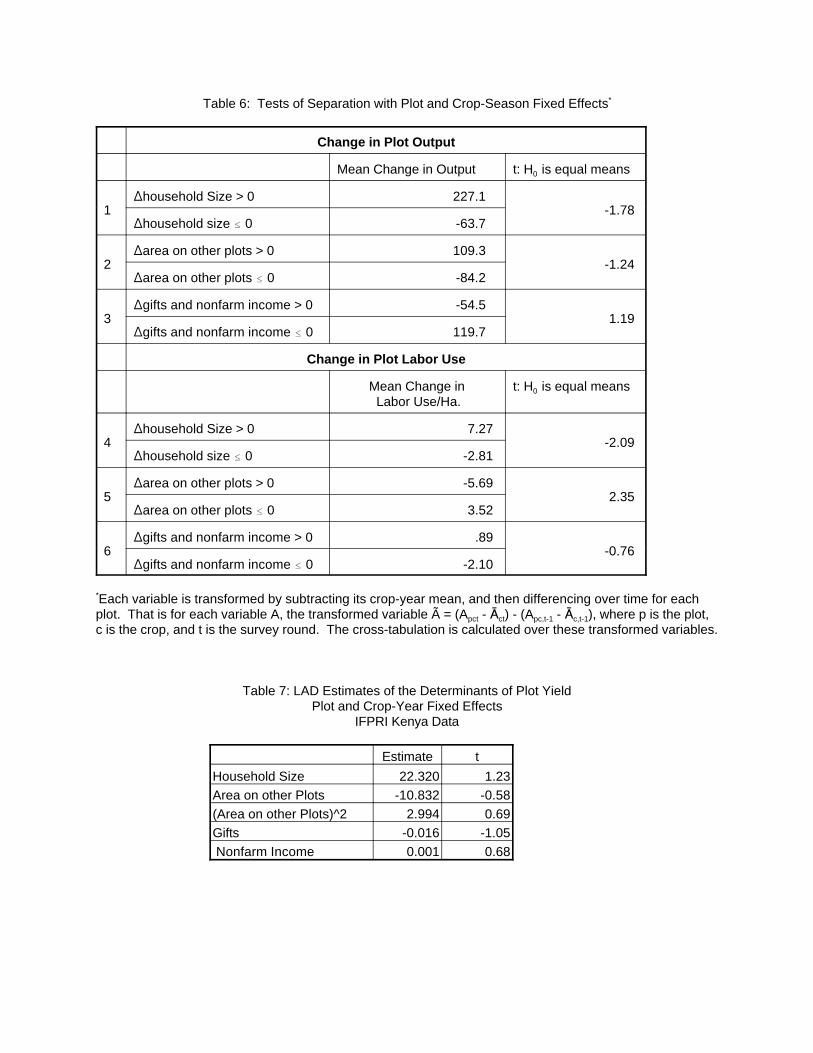
Table 6: Tests of Separation with Plot and Crop-Season Fixed Effects*

Change in Plot Output

Mean Change in Output t: H is equal means0

1 -1.78household Size > 0 227.1

household size 0 -63.7

2 -1.24area on other plots > 0 109.3

area on other plots 0 -84.2

3 1.19gifts and nonfarm income > 0 -54.5

gifts and nonfarm income 0 119.7

Change in Plot Labor Use

Mean Change in t: H is equal means Labor Use/Ha.

0

4 -2.09household Size > 0 7.27

household size 0 -2.81

5 2.35area on other plots > 0 -5.69

area on other plots 0 3.52

6 -0.76gifts and nonfarm income > 0 .89

gifts and nonfarm income 0 -2.10

Each variable is transformed by subtracting its crop-year mean, and then differencing over time for each*

plot. That is for each variable A, the transformed variable à = (A - ) - (A - ), where p is the plot,pct ct pc,t-1 c,t-1

c is the crop, and t is the survey round. The cross-tabulation is calculated over these transformed variables.

Table 7: LAD Estimates of the Determinants of Plot YieldPlot and Crop-Year Fixed Effects

IFPRI Kenya Data

Estimate tHousehold Size 22.320 1.23Area on other Plots -10.832 -0.58(Area on other Plots)^2 2.994 0.69Gifts -0.016 -1.05 Nonfarm Income 0.001 0.68