effects of weather on mosquito biology, behavior, and potential for ...
197
EFFECTS OF WEATHER ON MOSQUITO BIOLOGY, BEHAVIOR, AND POTENTIAL FOR WEST NILE VIRUS TRANSMISSION ON THE SOUTHERN HIGH PLAINS OF TEXAS by CARRIE MARIE BRADFORD, B.S., M.S. A DISSERTATION IN ENVIRONMENTAL TOXICOLOGY Submitted to the Graduate Faculty of Texas Tech University in Partial Fulfillment of the Requirements for the Degree of DOCTOR OF PHILOSOPHY Approved Steven Presley Chairperson of the Committee Todd Anderson Stephen Cox Nancy McIntyre Richard Nisbett Accepted John Borrelli Dean of the Graduate School AUGUST, 2005
Transcript of effects of weather on mosquito biology, behavior, and potential for ...

EFFECTS OF WEATHER ON MOSQUITO BIOLOGY, BEHAVIOR,
AND POTENTIAL FOR WEST NILE VIRUS TRANSMISSION
ON THE SOUTHERN HIGH PLAINS OF TEXAS
by
CARRIE MARIE BRADFORD, B.S., M.S.
A DISSERTATION
IN
ENVIRONMENTAL TOXICOLOGY
Submitted to the Graduate Faculty of Texas Tech University in
Partial Fulfillment of the Requirements for
the Degree of
DOCTOR OF PHILOSOPHY
Approved
Steven Presley Chairperson of the Committee
Todd Anderson
Stephen Cox
Nancy McIntyre
Richard Nisbett
Accepted
John Borrelli
Dean of the Graduate School
AUGUST, 2005

ACKNOWLEDGMENTS
First I would like to thank my major advisor, Dr. Steven Presley, for giving
me the opportunity to work on this project. He has taught me much over the
years, and I am grateful to him for introducing me to the field of vector-borne
disease epidemiology and ecology. I would also like to thank my committee
members, Drs. Stephen Cox, Todd Anderson, Nancy McIntyre, and Richard
Nisbett for their help and guidance throughout this study. I would also like to
thank The Institute of Environmental and Human Health at Texas Tech University
for financial support and the use of facilities and equipment.
I owe a great deal of gratitude to Drs. Stephen Cox and Clyde Martin for
their assistance in determining appropriate strategies for data analysis. I am also
thankful to Drs. James Surles and Ken Dixon for additional statistical help
provided. A special thank you also goes to Dr. Eric Marsland for taking the time
to train me in molecular procedures.
This project could not have been completed without the continued help
and support from the vector-borne zoonosis lab crew. A special thank you to the
members of our team, including Chris Pepper, Marc Nascarella, Drs. Eric
Marsland and Galen Austin, Robin Pollard, Teresa Burns, and John Montford.
All of these people were always available for help in mosquito collections,
mosquito identification, sample processing, and anything else that I needed help
with along the way.
I would also like to thank Wayne Gellido for providing data regarding
mosquito collections by the City of Lubbock, as well as Randy Apodaca, Adam
Finger, Les McDaniel, Toby McBride, Kevin Reynolds, Dub Parks Arena, Texas
Tech Equestrian Center, FOX 34 television, KRFE radio, Lubbock Christian
University, Meadowbrook Golf Course, Texas Tech Farm at New Deal, Reese
Redevelopment Commission, and The Windmill Museum for their aid in mosquito
collections or the use of their land for setting mosquito traps.
ii

I would also like to thank Dr. Todd Anderson, Jaclyn Canas, Aaron Scott,
and Nick Romero for technical assistance provided in the development of a
method for determining the effectiveness of mosquito control operations, and for
the use of laboratory equipment. In addition, Joe Vargas from the City of
Lubbock and Rick West at Texas Tech University provided information regarding
areas in which mosquito control operations would take place
I am especially thankful to Achievement Rewards for College Scientists
(ARCS) for providing me with a scholarship. In addition to the tremendous
financial support they provided, they also provided encouragement and renewed
my excitement about my project every time I talked with them. I would also like
to thank the Howard Hughes Medical Institute for providing financial support for
Robin Pollard to work during the summer. Additional financial support was
provided by Dr. Ron Warner at the Texas Tech Health Sciences Center and by
Dr. James Alexander at Region I, Texas Department of State Health Service.
Finally, I would like to thank my family and friends. I am especially
grateful to my husband, Brian Bradford, for his continued love, support, and
understanding over the last several years. I am also thankful for my parents,
Allan and Eunice Hendrickson, for their love and support throughout all of my
endeavors. I am also thankful to all of the faculty, staff, and students at The
Institute of Environmental and Human Health for everything they have done for
me on both the professional and personal level.
iii

TABLE OF CONTENTS
ACKNOWLEDGMENTS ii
ABSTRACT vii
LIST OF TABLES ix
LIST OF FIGURES xi
CHAPTER
I. INTRODUCTION AND RESEARCH GOALS 1
Emerging and Resurgent Vector-Borne Diseases 1
Global Climate Change and Vector-Borne Diseases 6
Research Goals and Hypotheses 12
II. ABIOTIC FACTORS AFFECTING WEST NILE
VIRUS MAINTENANCE AND TRANSMISSION:
CLIMATIC CHANGES OVER TIME 15
Introduction and Research Goals 15
Materials and Methods 17
Results and Discussion 18
Conclusions and Future Studies 21
III. BIOTIC FACTORS AFFECTING WEST NILE
VIRUS MAINTENANCE AND TRANSMISSION:
MOSQUITO COMMUNITY DYNAMICS IN
RESPONSE TO CLIMATIC CHANGE 23
Introduction and Research Goals 23
Mosquito Classification 23
iv

Mosquito Life Cycle and General Morphology 23
Mosquito Life History and Medical Importance 31
Mosquito Collection Methods 41
Research Goals and Hypotheses 46
Materials and Methods 47
Mosquito Collection and Identification 47
Weather Data 49
Analyses 50
Results and Discussion 50
Conclusions and Future Studies 85
IV. OVERALL INFLUENCES AND DRIVERS OF
WEST NILE VIRUS OCCURRENCE AND
TRANSMISSION 86
Introduction and Research Goals 86
Mosquitoes and Disease Transmission 86
West Nile Virus Classification and Structure 91
West Nile Virus History and Distribution 92
West Nile Virus in Mosquitoes 97
West Nile Virus Screening Methods 102
Research Goals and Hypotheses 106
Materials and Methods 106
Mosquito Collection and Identification 106
Weather Data 107
Screening for West Nile Virus 107
Analyses 112
Results and Discussion 113
Conclusions and Future Studies 134
v

V. PRELIMINARY STUDIES ON THE EFFECTS
OF PESTICIDES ON MOSQUITO COMMUNITIES
AND WEST NILE VIRUS MAINTENANCE
AND TRANSMISSION 135
Introduction and Research Goals 135
Materials and Methods 137
Results and Discussion 140
Conclusions and Future Studies 142
VI. CONCLUSIONS AND FUTURE RESEARCH 143
Study Summary and Conclusions 143
Future Studies to Address New Questions 145
REFERENCES 149
APPENDIX
A. CHARACTERIZATION OF MOSQUITO
TRAPPING SITES 162
B. EXPLANATION OF WEATHER LAGS USED IN
REGRESSION ANALYSIS 166
C. MANUFACTURER PROTOCOLS FOR WEST
NILE VIRUS SCREENING METHODS 170
vi

ABSTRACT
The threat of emerging and resurgent vector-borne diseases associated
with weather conditions, global climate change, and biologic attacks is of major
concern. West Nile virus (WNV) first appeared in the United States in the
summer of 1999. Since then it has spread rapidly across the nation and
continues to be a threat to humans, domestic animals (particularly horses), and
wildlife.
The goal of this project was to model the factors involved in the WNV
maintenance and transmission cycle. Mosquito surveillance to determine
mosquito community dynamics and WNV infection in mosquito populations has
been ongoing in Lubbock County, TX (33.65°N; 101.81°W; 975 m elevation),
since the summer of 2002. West Nile virus was first detected in Lubbock County
in late summer 2002 and has continued to appear each summer. The
occurrence of WNV in mosquitoes collected over a three-year period was
determined and related to very diverse annual weather conditions during those
years in order to determine trends in WNV occurrence.
Differences in weather conditions between study years was reflected in
differences in mosquito collections and WNV maintenance and transmission. In
the Lubbock area, 2003 was a drought year, and Culex tarsalis Coquillett
dominated mosquito collections due to an abundance of stagnant pools that
allowed for the proliferation of this species. Additionally, a large number of
mosquito pools tested positive for WNV. The following year, however, was a wet
year, and Aedes vexans Meigen, a floodwater species, dominated mosquito
collections. During 2004, the number of WNV-positive mosquito pools was
reduced by two-thirds, despite testing approximately the same number of pools.
Modeling mosquito populations and WNV occurrence in relation to weather
patterns revealed interesting trends. Both of these were predicted by weather
conditions, typically rainfall and temperature, in the weeks prior to collection of
vii
WNV infected mosquitoes. By understanding the factors that drive mosquito
populations and the occurrence of WNV, future patterns of disease occurrence
can be predicted and efficient mosquito control operations can be initiated prior
to a major disease outbreak.
Models which explain when and why disease transmission occurred are
important as related to effective surveillance and control activities as well as with
respect to climate change and the potential for biologic attacks. Climate change
is expected to increase the geographic distribution of many vector-borne
diseases, and especially mosquito-borne diseases. Malaria, among other
diseases, has already reappeared in regions in which it had previously been
eradicated. Global warming that is projected to occur with climate change will
allow for the geographic range of many mosquito species to be expanded, with
the potential for these species to carry new diseases into naïve areas.
Additionally, climate change is expected to increase the frequency of extreme
events such as floods and droughts, which have previously been shown to
facilitate the outbreak of various mosquito-borne diseases. Models of disease
transmission will help public health officials initiate effective surveillance and
proactive control strategies to prevent the further spread of disease. Acts of
terrorism involving biologics is also of major concern. Models of disease
transmission will aid in distinguishing between natural outbreaks of disease and a
biologic attack. Understanding how a disease outbreak was initiated is also
critical for effective surveillance and control operations, since biologic attacks
could involve genetically altered pathogens, thus potentially requiring a different
means of disease treatment or control.
viii
LIST OF TABLES
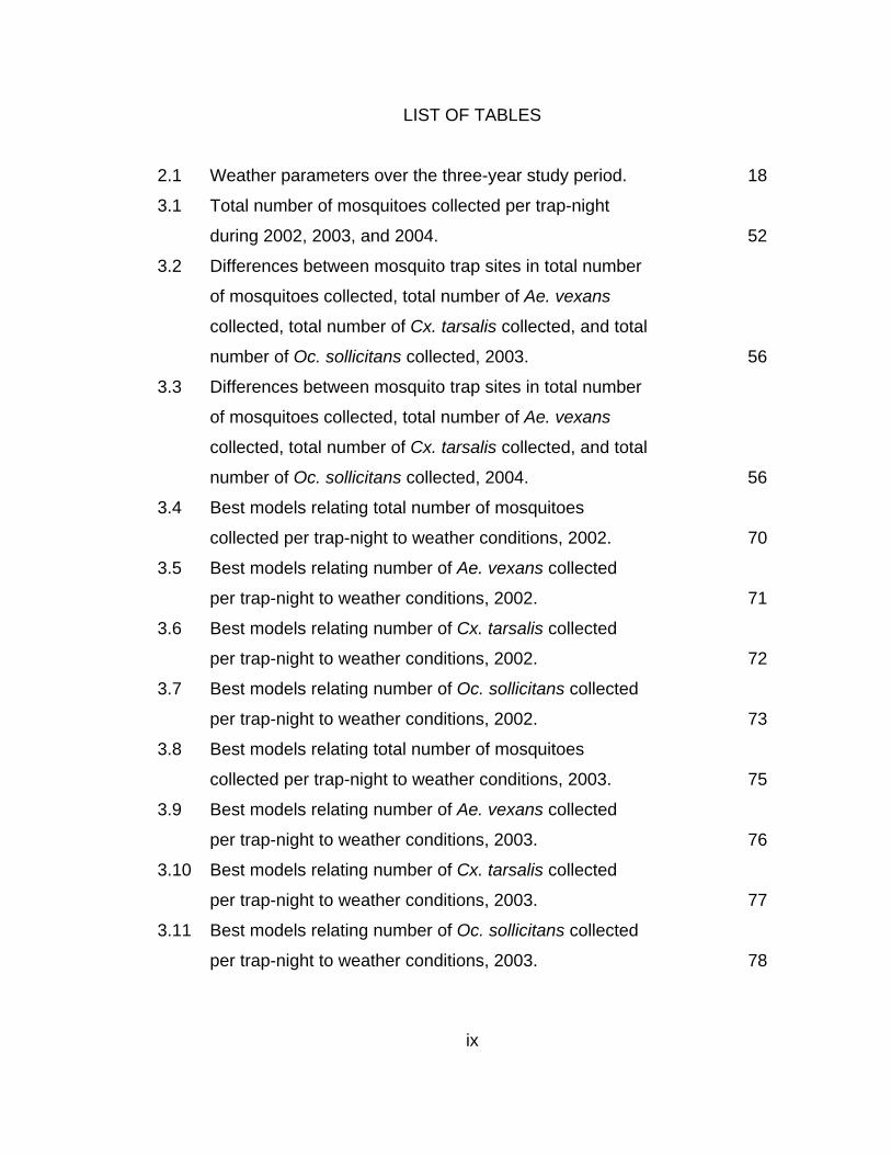
2.1 Weather parameters over the three-year study period. 18
3.1 Total number of mosquitoes collected per trap-night
during 2002, 2003, and 2004. 52
3.2 Differences between mosquito trap sites in total number
of mosquitoes collected, total number of Ae. vexans
collected, total number of Cx. tarsalis collected, and total
number of Oc. sollicitans collected, 2003. 56
3.3 Differences between mosquito trap sites in total number
of mosquitoes collected, total number of Ae. vexans
collected, total number of Cx. tarsalis collected, and total
number of Oc. sollicitans collected, 2004. 56
3.4 Best models relating total number of mosquitoes
collected per trap-night to weather conditions, 2002. 70
3.5 Best models relating number of Ae. vexans collected
per trap-night to weather conditions, 2002. 71
3.6 Best models relating number of Cx. tarsalis collected
per trap-night to weather conditions, 2002. 72
3.7 Best models relating number of Oc. sollicitans collected
per trap-night to weather conditions, 2002. 73
3.8 Best models relating total number of mosquitoes
collected per trap-night to weather conditions, 2003. 75
3.9 Best models relating number of Ae. vexans collected
per trap-night to weather conditions, 2003. 76
3.10 Best models relating number of Cx. tarsalis collected
per trap-night to weather conditions, 2003. 77
3.11 Best models relating number of Oc. sollicitans collected
per trap-night to weather conditions, 2003. 78
ix

3.12 Best models relating total number of mosquitoes
collected per trap-night to weather conditions, 2004. 80
3.13 Best models relating number of Ae. vexans collected
per trap-night to weather conditions, 2004. 81
3.14 Best models relating number of Cx. tarsalis collected
per trap-night to weather conditions, 2004. 82
3.15 Best models relating number of Oc. sollicitans collected
per trap-night to weather conditions, 2004. 83
4.1 Mosquito species that have tested positive for WNV
during 1999 through 2004 and those species that are
located in Lubbock County. 98
4.2 Total number of mosquitoes collected, total number of
mosquitoes screened, total number of WNV positive
results, and MIR, 2002. 113
4.3 Total number of mosquitoes collected, total number of
mosquitoes screened, total number of WNV positive
results, and MIR, 2003. 114
4.4 Total number of mosquitoes collected, total number of
mosquitoes screened, total number of WNV positive
results, and MIR, 2004. 115
4.5 Best models for MIR based upon weather conditions only, 2003. 126
4.6 Best models for MIR based upon weather conditions only, 2004. 127
4.7 Best models for MIR based upon weather conditions
and vector abundance, 2003. 129
4.8 Best models for MIR based upon weather conditions
and vector abundance, 2004. 130
A.1 Characterization of mosquito trapping sites. 163
B.1 Weather lags used in regression analysis. 167
x

LIST OF FIGURES
1.1 The relationship of emerging infectious diseases
among humans, wildlife, and domestic animals. 6
2.1 Smoothing spline transformation of average weekly
air temperature during 2002, 2003, and 2004. 19
2.2 Smoothing spline transformation of average weekly
relative humidity during 2002, 2003, and 2004. 19
2.3 Total weekly precipitation during 2002, 2003, and 2004. 20
2.4 Smoothing spline transformation of total weekly heat
units during 2002, 2003, and 2004. 20
2.5 Smoothing spline transformation of cumulative heat
units during 2002, 2003, and 2004. 21
3.1 The mosquito life cycle. 24
3.2 Mosquito egg raft. 25
3.3 Mosquito larvae. 26
3.4 Mosquito pupae. 27
3.5 Anatomy of the adult mosquito. 28
3.6 Mouthparts of the female adult mosquito. 29
3.7 Aedes vexans. 34
3.8 Culex tarsalis. 37
3.9 Ochlerotatus sollicitans. 39
3.10 Dry Ice® baited light trap set by Texas Tech University. 43
3.11 New Jersey light trap set by the City of Lubbock and
CDC ultraviolet light trap set by Texas Tech University. 44
3.12 Dipper for the collection of mosquito larvae. 46
3.13 Percentage generic composition of total number of
mosquitoes collected each year, 2002 through 2004. 53
xi
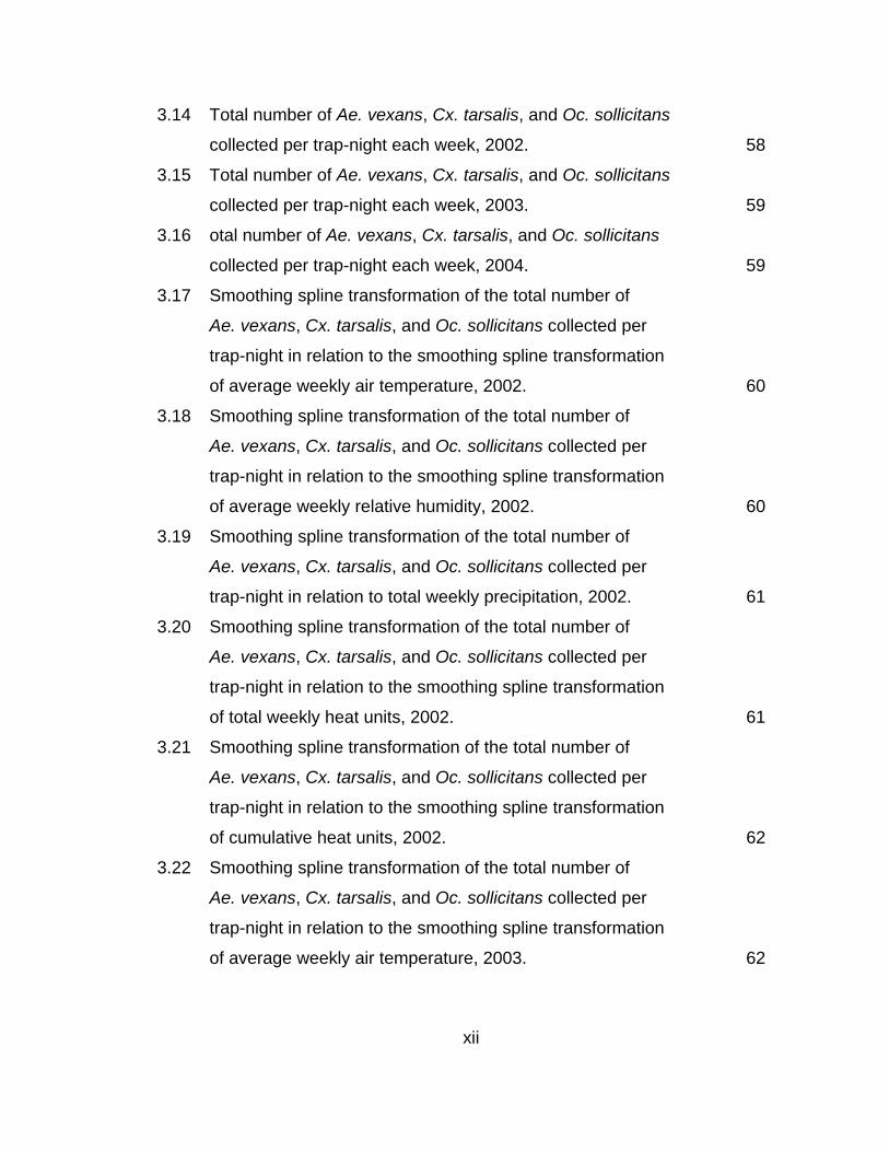
3.14 Total number of Ae. vexans, Cx. tarsalis, and Oc. sollicitans
collected per trap-night each week, 2002. 58
3.15 Total number of Ae. vexans, Cx. tarsalis, and Oc. sollicitans
collected per trap-night each week, 2003. 59
3.16 otal number of Ae. vexans, Cx. tarsalis, and Oc. sollicitans
collected per trap-night each week, 2004. 59
3.17 Smoothing spline transformation of the total number of
Ae. vexans, Cx. tarsalis, and Oc. sollicitans collected per
trap-night in relation to the smoothing spline transformation
of average weekly air temperature, 2002. 60
3.18 Smoothing spline transformation of the total number of
Ae. vexans, Cx. tarsalis, and Oc. sollicitans collected per
trap-night in relation to the smoothing spline transformation
of average weekly relative humidity, 2002. 60
3.19 Smoothing spline transformation of the total number of
Ae. vexans, Cx. tarsalis, and Oc. sollicitans collected per
trap-night in relation to total weekly precipitation, 2002. 61
3.20 Smoothing spline transformation of the total number of
Ae. vexans, Cx. tarsalis, and Oc. sollicitans collected per
trap-night in relation to the smoothing spline transformation
of total weekly heat units, 2002. 61
3.21 Smoothing spline transformation of the total number of
Ae. vexans, Cx. tarsalis, and Oc. sollicitans collected per
trap-night in relation to the smoothing spline transformation
of cumulative heat units, 2002. 62
3.22 Smoothing spline transformation of the total number of
Ae. vexans, Cx. tarsalis, and Oc. sollicitans collected per
trap-night in relation to the smoothing spline transformation
of average weekly air temperature, 2003. 62
xii
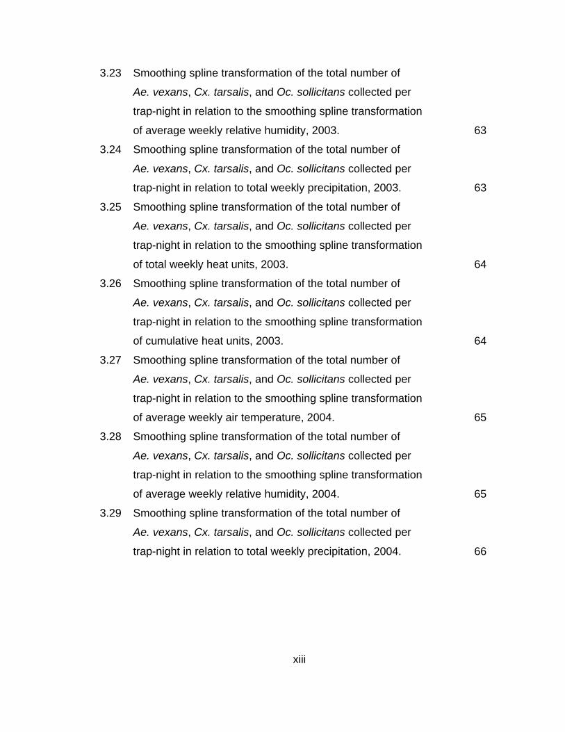
3.23 Smoothing spline transformation of the total number of
Ae. vexans, Cx. tarsalis, and Oc. sollicitans collected per
trap-night in relation to the smoothing spline transformation
of average weekly relative humidity, 2003. 63
3.24 Smoothing spline transformation of the total number of
Ae. vexans, Cx. tarsalis, and Oc. sollicitans collected per
trap-night in relation to total weekly precipitation, 2003. 63
3.25 Smoothing spline transformation of the total number of
Ae. vexans, Cx. tarsalis, and Oc. sollicitans collected per
trap-night in relation to the smoothing spline transformation
of total weekly heat units, 2003. 64
3.26 Smoothing spline transformation of the total number of
Ae. vexans, Cx. tarsalis, and Oc. sollicitans collected per
trap-night in relation to the smoothing spline transformation
of cumulative heat units, 2003. 64
3.27 Smoothing spline transformation of the total number of
Ae. vexans, Cx. tarsalis, and Oc. sollicitans collected per
trap-night in relation to the smoothing spline transformation
of average weekly air temperature, 2004. 65
3.28 Smoothing spline transformation of the total number of
Ae. vexans, Cx. tarsalis, and Oc. sollicitans collected per
trap-night in relation to the smoothing spline transformation
of average weekly relative humidity, 2004. 65
3.29 Smoothing spline transformation of the total number of
Ae. vexans, Cx. tarsalis, and Oc. sollicitans collected per
trap-night in relation to total weekly precipitation, 2004. 66
xiii

3.30 Smoothing spline transformation of the total number of
Ae. vexans, Cx. tarsalis, and Oc. sollicitans collected per
trap-night in relation to the smoothing spline transformation
of total weekly heat units, 2004. 66
3.31 Smoothing spline transformation of the total number of
Ae. vexans, Cx. tarsalis, and Oc. sollicitans collected per
trap-night in relation to the smoothing spline transformation
of cumulative heat units, 2004. 67
4.1 Estimate of world malaria burden, with intensity of blue
indicating increasing burden of malaria. 89
4.2 Life cycle of Plasmodium spp. in human and Anopheles hosts. 90
4.3 The approximate geographic range of WNV as of 2002. 93
4.4 The spread of WNV across the United States,
1999 through 2004. 95
4.5 Texas counties with WNV-positive bird, mosquito, horse,
other animal, or human cases, 2002 through 2004. 96
4.6 A representative 2% agarose gel displaying
WNV-positive results from RT-PCR. 111
4.7 A representative VecTest® assay indicating a
WNV-positive result. 112
4.8 Total number of WNV-positive mosquito pools by week,
2002 through 2004. 116
4.9 Weekly MIR in relation to the smoothing spline
transformation of average weekly air temperature, 2003. 117
4.10 Weekly MIR in relation to the smoothing spline
transformation of average weekly relative humidity, 2003. 118
4.11 Weekly MIR in relation to total weekly precipitation, 2003. 118
4.12 Weekly MIR in relation to the smoothing spline
transformation of total weekly heat units, 2003. 119
xiv

4.13 Weekly MIR in relation to the smoothing spline
transformation of cumulative heat units, 2003. 119
4.14 Weekly MIR in relation to the smoothing spline
transformation of total number of mosquitoes
collected per trap-night, 2003. 120
4.15 Weekly MIR in relation to the smoothing spline
transformation of total number of Cx. tarsalis
collected per trap-night, 2003. 120
4.16 Weekly MIR in relation to the smoothing spline
transformation of average weekly air temperature, 2004. 121
4.17 Weekly MIR in relation to the smoothing spline
transformation of average weekly relative humidity, 2004. 121
4.18 Weekly MIR in relation to total weekly precipitation, 2004. 122
4.19 Weekly MIR in relation to the smoothing spline
transformation of total weekly heat units, 2004. 122
4.20 Weekly MIR in relation to the smoothing spline
transformation of cumulative heat units, 2004. 123
4.21 Weekly MIR in relation to the smoothing spline
transformation of total number of mosquitoes
collected per trap-night, 2004. 123
4.22 Weekly MIR in relation to the smoothing spline
transformation of total number of Cx. tarsalis
collected per trap-night, 2004. 124
5.1 Stake and mosquito cage containing live mosquitoes
with sample papers attached to the top for collection
of residues from mosquito control pesticide applications. 138
5.2 Stability of permethrin and malathion under environmental
conditions from 0 to 12 hours. 140
xv
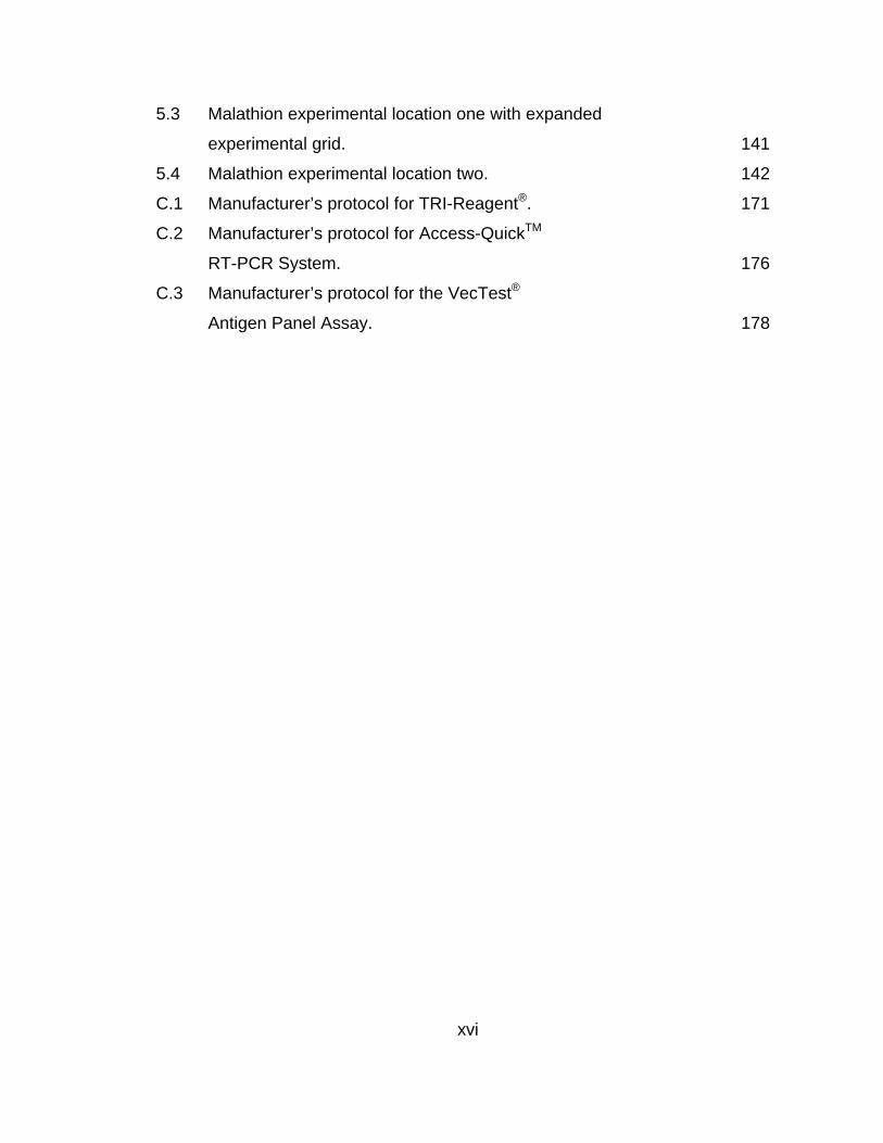
5.3 Malathion experimental location one with expanded
experimental grid. 141
5.4 Malathion experimental location two. 142
C.1 Manufacturer’s protocol for TRI-Reagent®. 171
C.2 Manufacturer’s protocol for Access-QuickTM
RT-PCR System. 176
C.3 Manufacturer’s protocol for the VecTest®
Antigen Panel Assay. 178
xvi

CHAPTER I
INTRODUCTION AND RESEARCH GOALS
Emerging and Resurgent Vector-Borne Diseases
During the 1970s, physicians and scientists began to believe that
infectious diseases were on the decline [1]. By 1975, smallpox had been virtually
eradicated, and tuberculosis and polio, along with most other infectious diseases
besides malaria, were on the decline due to improved hygiene and sanitation as
well as immunizations and antibiotics [1]. However, agents of these diseases
were beginning to show resistance to antibiotics, and some diseases of plants
and animals were beginning to appear in other plant and animal species (in
which previous infection had not been seen) with devastating effects [1].
One example of a vector-borne disease crossing over into a new species
is that of scrapie. Scrapie, typically a mild disease in sheep, was found infecting
cattle, resulting in cattle deaths [1]. Additionally, Lyme disease, Legionnaire’s
disease, toxic shock syndrome, and hantavirus among other diseases began to
appear in human populations in the 1970s and following decades. A new variant
of cholera emerged as a pandemic that began in Indonesia in 1961. In recent
years, malaria has reappeared in regions where it had previously been
eradicated, tuberculosis incidence is increasing in areas that had previously seen
a decline, and dengue and yellow fever are also increasing in their geographic
reach [1]. Reasons for this phenomenon could be linked to increased resistance
of the vector population to insecticides, increased resistance of the pathogen to
therapeutic treatment, or to a changing environment due to both natural variation
and anthropogenic impacts [1].
Today, the scientific community does not believe that all diseases can
eventually be eradicated, but rather that there will be a pattern of disease cycling
and that infectious diseases will always be a part of human life [1]. Instead of
focusing on how to fight diseases as they arise, scientists are now concentrating
1

their efforts by investigating factors that lead to the emergence and spread of
these diseases. Social, epidemiological, ecological, and evolutionary processes
are being integrated to form an understanding of how these factors influence
infectious diseases. The history and progression of existing diseases are
evaluated in an effort to predict when and where emergent or resurgent diseases
may appear [1].
Emerging and resurgent infectious diseases are a great threat to human
and animal health [2]. Emerging infectious diseases include those that have
previously gone undetected, diseases in which their geographic range has been
extended, or diseases whose incidence has increased over the last decade,
whereas resurgent infectious diseases refer to diseases that exhibit an
increasing incidence in an area that previously experienced a decline in
incidence [2]. In both emerging and resurgent infectious diseases, there is an
increased presence of disease agents. Examples of emerging and resurgent
infectious agents include filoviruses, hantaviruses, flaviviruses, and plague [2].
Modern transportation has facilitated the introduction and may have
contributed to the maintenance of many infectious agents [1]. One important
factor to consider is the relationship between the travel time to get to an area and
the incubation period for a specific pathogen. When international travel was
slower, the spread of diseases such as smallpox was hindered because most
infected people began to show symptoms of disease or may have even died
before reaching their destination. Today, travel to practically anywhere in the
world can be accomplished in a few days or less, allowing humans to be the
carriers of diseases into new areas without even knowing they are infected [1].
There are many factors that influence disease resurgence, some of which
include changes at the social, ecological, and global level [3]. Social changes
include the excessive use of antibiotics and pesticides, and economic disparities.
At the ecological level, there is habitat loss, and habitat integrity is essential for
diversity that allows for resilience to stress and resistance to pathogens.
2
Globally, there are changes in climate and stratospheric ozone [3]. The spread
of arthropod vectors of disease from tropical areas into temperate areas, which
may contribute to the emergence and resurgence of disease, has been facilitated
by increases in populations and urbanization, degradation of the natural
environment, and international trade and travel [4]. Together, all of these factors,
which are dependent on each other, have influenced the current status of vector-
borne diseases [5].
Increased human contact with disease vectors combined with global
climate change have attributed to the appearance of many new vector-borne
diseases, as well as an increased geographic range and incidence of endemic
diseases [6]. Emerging and resurgent vector-borne diseases present challenges
to public health officials in that they must identify these new pathogens and their
potential vectors, understand the dynamics of their maintenance and
transmission, and investigate the numerous factors that may be responsible for
the new outbreaks [6].
Some of the vector-borne diseases that have recently come into the
spotlight are arboviruses, which include flaviviruses. Of most recent particular
concern is West Nile virus (WNV), the most geographically widespread of the
flaviviruses [7]. In addition to being an emerging pathogen in the New World and
a resurgent pathogen throughout the world, there is also concern regarding
epidemiologic trends that have been realized since the mid-1990s [8].
Traditionally, WNV outbreaks throughout the world have infrequently occurred in
humans. Recently, however, in the United States and in other countries
throughout the world, there has been an increase in the frequency of disease
outbreaks in humans and horses, an increase in the severity of human disease,
and high avian death rates associated with the human outbreaks. These new
trends appear to be due to the evolution of a new WNV variant [8].
The evolution of pathogens, including adaptation of the pathogen for
growth within humans and the subsequent transmission of the pathogen between
3

humans, describes the increase in virulence of diseases caused by these
pathogens [9]. Typically for a disease to successfully emerge, the basic
reproductive number of the pathogen must exceed one in the new host, which
also means an epidemic may occur. If the basic reproductive rate remains less
than one, an epidemic will not occur because infections will die out [9].
Ecological changes of the pathogen that result in the slight increase of the basic
reproductive number, but not to a level that leads to an epidemic, increases the
amount of disease transmission and the ability of the disease to emerge as
pathogens are given the opportunity to adapt to human hosts. The probability of
pathogen evolution and the probability that evolved infections do not become
extinct determine whether the disease emergence results in an epidemic [9].
Recent studies demonstrate that the majority of pathogens causing human
disease are zoonotic, and zoonotic species are twice more likely than non-
zoonotic pathogens to be associated with emerging diseases [10]. Among these,
viruses and protozoa are most likely to emerge due to their biology, including
genetic diversity and generation time of these pathogens. This indicates
taxonomic and zoonotic status to be the driving factors for risk of disease
emergence, but does not consider the severity of these diseases [10].
Over 50 emergent pathogens have been reported by the Centers for
Disease Control and Prevention (CDC) and the World Health Organization
(WHO) in the last 30 years [2]. The list of these emerging pathogens becomes
longer when pathogens that could be used as biological weapons are included.
Among those that could be used as biological weapons are pathogens which
pose a high risk to an individual or a community, and many are zoonotic diseases
[2]. These potential biological agents have been classified based upon their
potential for use and effectiveness. Category A agents are pathogens that have
the greatest potential for adverse public health impacts and a moderate to high
potential for large-scale dissemination, including pathogens such as smallpox
(Variola major), anthrax (Bacillus anthracis), plague (Yersinia pestis), tularemia
4
(Francisella tularensis), and hemorrhagic fevers (filoviruses). Category B agents
have the same potential for large-scale dissemination as do Category A agents,
but have reduced morbidity and mortality, including pathogens such as Q fever
(Coxiella burnetii), brucellosis (Brucella spp.), glanders (Burkholderia mallei),
viral encephalitides, typhus fever (Rickettsia prowazekii), biological toxins (ricin),
and food and water safety threats (Escherichia coli, Salmonella spp., and Vibrio
cholerae). Category C agents are those that may emerge as future health
threats and include pathogens such as hantaviruses, tick-borne encephalitis
viruses, tick-borne hemorrhagic fever viruses, and yellow fever [2].
In addition to the threat to human health from both naturally occurring
emerging and resurgent vector-borne diseases, and from potential attacks with
biologics, these pathogens are also a threat to domestic animals and wildlife.
Figure 1.1 modified from Daszak and others [11] depicts the intimate relationship
between humans, domestic animals, and wildlife with emerging infectious
diseases. Emerging infectious diseases are particularly a threat to endangered
species because of the risk of extinction. Although the extinction of a species in
itself may be devastating to a particular region, the threat of reduced global
biodiversity is more worrisome [11]. Maintenance of biodiversity is important for
keeping food webs and chains intact, and, because the exact role of many
species in an ecosystem is unknown, loss of a single or several species may
cause the entire ecosystem to suffer [12]. Additionally, high biodiversity provides
a rather large pool of genetic and pharmaceutical materials or organisms that
could potentially be used for medication or pest control, an issue that is important
with increasing drug and pest resistance [12]. Human introductions of nonnative
flora and fauna have already been shown to lead to biogeographical
homogeneity. Similarly, the introduction of a pathogen into a naïve population
may also lead to a loss of biodiversity as well as habitat loss [11].
5

Figure 1.1. The relationship of emerging infectious diseases among humans,
wildlife, and domestic animals. Arrows indicate key factors that drive the
emergence or resurgence of disease. Modified from Daszak and others [11].
Global Climate Change and Vector-Borne Diseases
One factor that may be driving emerging and resurgent diseases is global
climate change. Climate change over time occurs in continuous cycles [13].
Analysis of how these cycles occur was conducted by using the Sargasso Sea
record of sea surface temperature. Temperatures affect the ratio of different
oxygen isotopes taken up by marine organisms. As these organisms die and
sink to the sea floor, an integrated historic record of daytime surface water
temperature remains [13]. Due to the rapid sedimentation of the Sargasso Sea,
historic temperatures for every 67 years over a 3100-year period (1125 BC to
1975 AD) could be determined. Time-series analysis was then used to model
the climatic cycles in temperatures as a function of time. The data on historical
temperatures accounted for the major warming and cooling events (Medieval
Warm Period – 800 to 1200 AD and Little Ice Age – 1500 to 1850 AD) that
occurred in Europe. Models indicated a 500-year cycle of temperatures and that
6
the 20th century warming trends currently being observed are a continuation of
past climate patterns [13].
Global climate change may be attributable to both natural and
anthropogenic causes. Models have indicated that climate change is a result of
both natural climatic variability as well as anthropogenic forces from increased
atmospheric greenhouse gases and sulfate aerosols [14]. These models also
indicate that global warming during the first half of the 20th century was likely due
to natural climate variability whereas change in the second half of the 20th
century was due to human influence. Anthropogenic forcings in the second half
of the 20th century led to temperature changes, including overall changes in
average temperature as well as changes in the temperature gradient between
the northern and southern regions, temperature contrasts between land and
ocean, and reduced ranges of daily temperatures [14]. However, other studies
indicate that it is not yet possible to distinguish between the anthropogenic and
natural causes of climate change and that both contribute to climate change [13,
15, 16].
Ecological processes are influenced by climate, and attention recently has
turned to large-scale impacts of climate change on these ecological processes
on interannual and longer time scales [17]. Climate variation has both direct and
indirect influences on ecological processes. Direct influences involve changes in
an organism’s physiology, including reproductive and metabolic processes
whereas indirect influences involve changes in the ecosystem and the
relationships among prey, predators, and competitors [17]. Delayed effects of
climate occur in both marine and terrestrial ecosystems, and effects are variable
depending on an organism’s sex and age-class. Additionally, climate change is
likely to increase the frequency of extreme events, which have more of an impact
on ecosystems than do fluctuations in climate [17].
Climate affects the distribution of vector-borne diseases whereas weather
affects the timing and intensity of outbreaks of these diseases. Climate limits the
7

distribution of vectors, such as mosquitoes, to areas where temperatures remain
in a certain range; thus, climate limits the range of diseases transmitted by these
vectors [18]. Weather, such as temperature and precipitation, affects the biology
of the vector [19]. Extreme weather events, such as hurricanes, not only inflict
damage and death upon the area but also contribute to the outbreak of many
diseases, especially mosquito-borne diseases. During the major El Niño event of
1997 and 1998, the Horn of Africa received up to 40 times the average
precipitation, resulting in major epidemics of malaria and Rift Valley fever [3].
Global climate change has the potential to cause profound effects on
infectious diseases. While the diseases most likely to be influenced by climatic
change include vector-borne diseases such as dengue and yellow fever, water-
borne diseases such as cholera will also be affected [20]. Vector-borne diseases
are of concern because the distribution of these diseases is ultimately limited by
temperature and precipitation, as the range of the vector and/or vertebrate host is
limited by temperature and precipitation. Although the precise effect of climate
change on infectious diseases depends on the extent of weather changes that
may occur, the epidemiology of diseases can be used to predict how these
changes will affect human health [20].
Climate, vector ecology, and human social economics vary worldwide and
thus vector-borne diseases display regional variation [21]. In the tropics and
subtropics, malaria and dengue are a few of the most common vector-borne
diseases. In Europe and the United States, Lyme disease as well as various
encephalitis viruses are a major concern. Regions in which temperatures are
already at the extreme for disease transmission are likely to show the greatest
effects due to climate change [21]. In fact, in some areas, transmission of vector-
borne diseases may actually be reduced when temperatures exceed the
maximum range for vectors. This has already been seen in Senegal, where
malaria prevalence has dropped more than 60% and the predominant vector has
virtually disappeared from the area over the last 30 years [21].
8

Examination of the histories of malaria, yellow fever, and dengue reveals
that previous epidemics of these diseases have rarely been caused by climate
but rather by human activities and their impacts on the local ecology [22]. For
example, in South America, the cessation of house spraying with insecticides
faciliated outbreaks of malaria. Outbreaks of yellow fever in the early 20th
century were associated with the rapid growth of townships, especially in West
Africa. Additionally, immunization programs in French territories led to a
dramatic reduction in the prevalence of human disease in the 1940s and 1950s;
however, despite their success, these programs were discontinued in the 1960s
and since then, the frequency of outbreaks has been increasing [22]. The risk of
dengue transmission has also increased due to failure of mosquito control
operations, rapid growth of urban populations, and international air travel. In the
future, regions in which people are highly mobile are likely to be at risk of the
introduction of new diseases through international travel, and areas of declining
economies and political instability are at risk because of inadequate public health
programs [22]. Additionally, the mass migration of humans from rural areas to
coastal urban settings is evident globally by the number of large cities located
near the coast.
Mosquito-borne diseases are among the diseases in which there is much
concern because mosquitoes are extremely sensitive to weather conditions.
Cold conditions limit the range of mosquitoes and disease transmission [23].
Alternatively, warmer conditions, such as those that could be produced by global
warming, cause the disease transmission cycle to occur more rapidly due to
increases in both the rate of larval development and the extrinsic incubation
period of diseases [20]. This, in turn, would increase the speed of epidemic
spread of disease (assuming adequate water exists for continued mosquito
breeding). The range of vectors is also likely to expand northward and
southward as temperatures increase [20]. In addition to increasing temperatures,
global warming could also lead to intensified floods and droughts, which create
9

breeding sites for mosquitoes. Receding water from floods leaves puddles, and
streams become stagnant pools during droughts. Additionally, people may set
out containers that collect water. All of these make suitable breeding and
development areas for mosquitoes [23].
Although global warming itself would undoubtedly have significant effects
on vector-borne diseases, the increased transmission of these diseases may be
influenced more by the increased climatic variability associated with the warming.
Vectors of disease, especially mosquito vectors, are very diverse in their biology,
with some species preferring extremely wet climates and others preferring
extremely dry climates. Increased climatic variability could potentially lead to
increased variability in mosquito communities and thus in diseases transmitted
by these different species.
Vector-borne diseases have already been shown to be affected by
atypical weather conditions [23, 24]. Mosquito-borne diseases such as St. Louis
encephalitis (SLE) thrive in conditions of warm winters followed by hot, dry
summers. These conditions have already been shown to facilitate the
emergence of new diseases in the United States when WNV first appeared in
New York in 1999 [23]. Similarly, hantavirus began to appear in humans in the
early 1990s due to long-lasting droughts interrupted by intense rains [23]. This
typically rodent-borne disease made the jump into the human population when a
drought in the southwestern United States reduced the population of rodent
predators. Heavy rainfalls increased vegetation and insect populations, which
led to an increase in the rodent populations and an increased likelihood of human
exposure to the rodent-borne virus. Drought conditions during the following
summer caused the rodents to seek food in human dwellings and disease was
introduced into the human population [23]. Another example is that of Lyme
disease. In the northeastern United States, early summer Lyme disease
incidence was positively correlated with the June moisture index in the previous
two years for the region. It is thought that this phenomenon occurs because
10

drought conditions affect nymph tick survival, which would result in a reduced
population of egg-laying adults and the next nymph generation [24].
One mosquito-borne disease of particular concern is malaria. The
geographic range of malaria is smaller than its potential range based on the
geographic distribution of vector populations, a phenomenon referred to as
“Anophelism without malaria” [25]. Models of malaria risk indicate that these
areas, in which the vector exist but malaria transmission is limited by
temperature, are areas in which increased malaria transmission may occur in the
future with increased temperatures due to climate change [25]. Models estimate
that by the end of the 21st century, the region of potential malaria transmission
will increase from 45% of the world’s population to about 60% due to climate
change [23]. Other studies have shown that these models are too simplistic and
may exaggerate the risk of malaria resurgence [26] or that even under the most
extreme scenarios, there will be few changes in malaria distribution [27].
Already, malaria has begun to reappear in areas to the north and south of the
tropics, and during the 1990s, when the United States was experiencing one of
the hottest decades on record, outbreaks of locally transmitted malaria occurred
in Texas, Florida, Georgia, Michigan, New Jersey, and New York [23]. As
temperate areas become warmer and more humid with climate change, the risk
of malaria will increase. The tropical highlands of Africa, typically a defense
against malaria because of the lower temperatures, are also at risk for the
introduction of malaria, even with only a minor temperature increase [28].
The range of dengue fever is also expanding [23]. Previously limited in its
range by the 10°C winter isotherm at an elevation of 1000 m, the disease has
now been detected at 1700 m in Mexico and the vector of the disease has been
found at 2200 m in Columbia [18]. Climate models with dengue have shown that
epidemic potential increased with a small increase in temperature, indicating that
dengue could be spread and maintained in a vulnerable population with fewer
mosquitoes [29]. Additionally, fringe zones (nonendemic regions bordering
11

endemic areas) consist of both susceptible human populations and the vector,
but transmission is limited because of temperature. Outbreak of dengue in these
areas may be more severe because the population lacks immunity from prior
exposure [29].
Nonetheless, major factors in the eradication of malaria, dengue, and
other mosquito-borne diseases are human changes in lifestyle and living
conditions [19]. Unless the standard of living severely declines, these factors will
remain dominant in controlling vector-borne diseases. Rising temperatures will
force many people to seek shelter indoors, decreasing the risk of transmission of
these diseases. However, diseases will continue to reappear in urban areas, and
international travel will aid in spreading these diseases to new areas. Because of
this, there is a continued need for research to understand the interactions among
the vectors and vertebrate hosts and the habitat in which these interactions
occur, as well as continued surveillance for vector-borne diseases [19].
Research Goals and Hypotheses
The threat of emerging and resurgent vector-borne diseases associated
with weather conditions, global climate change, and biologic attacks is of major
concern. West Nile virus first appeared in the United States in the summer of
1999. Since then it has spread rapidly across the nation and continues to be a
threat to humans, domestic animals, wildlife, and particularly horses.
The goal of this project was to determine and model the factors involved in
WNV transmission. By understanding the factors (including weather conditions,
landscape features, and vector populations) that drive mosquito abundance and
the occurrence of WNV, future patterns of disease maintenance and
transmission can be predicted and efficient mosquito control operations can be
initiated prior to a major disease outbreak. Additionally, understanding when and
why disease outbreaks occur could be useful in differentiating between a
naturally occurring outbreak of disease and a biologic attack. It is hypothesized
12

that weather conditions, especially rainfall, in the weeks prior to mosquito
collection will influence mosquito community dynamics, and that collections of
vector species will influence occurrence of WNV infections.
Mosquito surveillance to determine mosquito community dynamics and
WNV infection in mosquito populations has been ongoing in Lubbock County, TX
(33.65°N; 101.81°W; 975 m elevation), since the summer of 2002. West Nile
virus was first detected in Lubbock County in late summer 2002 and has
continued to appear each summer; therefore, the occurrence of WNV in
mosquitoes collected over a three-year period was determined and related to
very diverse annual weather conditions during those years in order to recognize
influencing factors and determine trends in WNV occurrence.
Lubbock, TX, is an excellent location for the study of vector-borne
diseases and especially mosquito-borne diseases such as WNV. In West Texas,
weather conditions are highly variable throughout the year with the potential for
warm days during the winter months and cool days during summer months. The
area is also known to have both torrential rainfall as well as severe drought. The
Southern High Plains of the United States, including most of West Texas, is
dotted with playa lakes, which are hollows in the ground that collect runoff from
irrigation and rainfall. Although playa lakes are considered to be temporary
bodies of water, many of them hold at least a small amount of water year-round.
With the combination of a large number of playa lakes and drainage basins
throughout the city and county, the area has standing water in both rural and
urban areas, allowing for the proliferation of mosquitoes year-round.
An additional study was conducted to gather preliminary data regarding
the environmental effects of mosquito control programs and agricultural pesticide
applications. The city of Lubbock is surrounded by an agricultural community
where pesticides are used regularly to control pests of crops. The goal of this
preliminary study was to develop methods for determining the effectiveness of
mosquito control operations and to apply those methods to agricultural
13

communities to determine the effects of agricultural pesticides on mosquito
communities and how that might possibly influence WNV transmission.
Insecticide residues were detected from samples collected from study sites
established at predetermined locations at or near the routes traveled during
mosquito control operations. The concentrations of these residues were related
to both the chemical applicator’s driving route and the wind direction during
spraying.
14

CHAPTER II
ABIOTIC FACTORS AFFECTING WEST NILE VIRUS MAINTENANCE AND
TRANSMISSION: CLIMATIC CHANGES OVER TIME
Introduction and Research Goals
Weather refers to the meteorological conditions at the present time and
place whereas climate refers to the typical regional conditions over an extended
period of time [30]. Weather is influenced by changes in wind patterns
throughout the world, and the many factors involved in weather, such as jet
stream, sea temperature, and barometric pressure systems, make weather
beyond the next few days difficult to predict. Climate, on the other hand, is
influenced by the intensity and patterns of solar energy, which are a function of
latitude, and climate for a given region for the next decade can be relatively
accurately predicted [30].
Although weather is highly variable, climate also changes over time [30].
On one time scale, glacial and interglacial oscillations change the climate of a
given region. Over the last four million years, scientists estimate that there have
been at least 22 ice ages (glacial periods) separated by relatively brief
interglacial periods [30]. During these glacial periods, air temperatures were
approximately 4 to 9°C cooler than present-day temperatures, which resulted in
ice sheets covering Canada and sea levels lowered by 125 m. On another time
scale, interannual climatic variability over the last several centuries has been
linked to oceanic conditions off the coast of Peru [30]. Typically, in December, a
warm ocean current from the Southern Oscillation appears near Peru. Although
the current usually fades early into the next year, the warm water may last until
July, an event that is called an El Niño event. The strongest El Niño event ever
recorded occurred in 1997/1998 [30]. El Niño typically brings torrential rainfall to
South America, but during this particular event, climate changes in North
America, Europe, and Asia were also observed. The El Niño Southern
15

Oscillation caused these widespread effects by displacing the polar jet stream,
which led to mild winters in North America. Following this major El Niño event,
waters in the Pacific Ocean were colder than usual, indicating a La Niña event,
and severe winters in the northern hemisphere were observed [30].
Climate changes over the last several decades have been observed.
Globally, 15 of the years between 1980 and 2000 were among the hottest on
record since 1881 when temperature observations were begun, and the hottest
years on record were 1997 and 1998 [31]. Despite the large amount of weather
data available through weather stations, ships’ logs, ocean buoys, and satellites,
collection of weather data was not standardized and accurate instrumentation
was not available until late in the 19th century. Still, patterns throughout the 20th
century indicate a cycling of warm and cool years. Models of future climate
change predict not only a general warming trend, but that climate will become
more erratic and that seasonality will become more pronounced [31].
Climate models for the 21st century predict both an increase in climate
variability as well as extreme events [32]. Warming is expected to occur
throughout North America, and most of the warming is predicted to occur during
the Arctic winter. Models predict a two- to ten-fold increase in warming during
the 21st century as compared to the 20th century, with temperatures increasing by
1.4 to 5.8°C, which would cause sea levels to rise 0.09 to 0.88 m by 2100 [32].
Additionally, precipitation is expected to increase in northern Canada and Alaska,
as well as a slight increase in winter precipitation in the eastern and western
United States. In Mexico, however, reduced precipitation is expected [32]. More
important for wildlife and ecosystems are the predicted changes in climatic
variability and extreme events. Models predict more hot extremes and fewer cold
extremes, as well as the increased intensity of extreme precipitation events and
more summer droughts [32].
The objective of this portion of the research project was to determine and
characterize the extent of interannual weather variation throughout a three-year
16

study period (2002, 2003, and 2004). Weather conditions for each year of this
study were analyzed and compared to the other study years and to 30-year
averages for the area. Understanding interannual variation of weather and its
effects upon mosquito community dynamics and West Nile virus (WNV)
maintenance and transmission is key to predicting future outbreaks of disease
and initiating mosquito control campaigns to prevent the further spread of
dissease.
Materials and Methods
Daily weather data from the Lubbock area (33.65°N; 101.81°W; 975 m
elevation) were obtained from the United States Department of Agriculture,
Agricultural Research Service, located in Lubbock, TX [33]. Weather parameters
included daily precipitation, average daily relative humidity, and average daily air
temperature (2 m above soil). Heat units were calculated as the average of daily
minimum and maximum temperatures minus the average mosquito
developmental threshold temperature of 15.56°C. The developmental threshold
temperature was based upon developmental rates of Culex pipiens Linnaeus and
Aedes vexans Meigen [34]. Heat units were calculated daily, and if the daily heat
unit was a negative number, the heat unit value for that day was changed to
zero. Heat units were summed to obtain the cumulative heat units for each year.
Thirty-year averages for climatic conditions in Lubbock were obtained from the
National Oceanic and Atmospheric Administration, National Climatic Data Center
[35]. These averages included air temperature, precipitation, freeze dates, and
heating and cooling degree days.
Smoothing spline transformations (smoothing parameter = 50) were
performed on weather data in order to remove “noise” in the data set and obtain
a curve of the general weather patterns. All analyses were conducted using SAS
version 9.1 (SAS Institute, Inc., Cary, NC) and graphical displays were produced
using SigmaPlot version 2000 (Systat Software Inc., Richmond, CA).
17

Results and Discussion
The goal of this portion of the research project was to determine
differences in weather patterns over the study period and to relate those
differences to 30-year averages for the Lubbock, TX, area. Weather data for the
study period are summarized in Table 2.1. Smoothing spline transformations
were used to obtain a view of differences in weather conditions between years
over weeks. Figures 2.1 through 2.5 illustrate the weekly differences in weather
conditions over the study years.
Table 2.1. Weather parameters over the three-year study period. Air
temperature and relative humidity are the averages ± standard deviation over
each year. Precipitation and heat units are cumulative for each year. Thirty-year
averages were obtained from the National Climatic Data Center [35]. 30-y Average 2002 2003 2004
Air Temperature (°C) 15.39 15.90 ± 9.23 16.70 ± 8.75 16.11 ± 8.39
Relative Humidity (%) NA 52.88 ± 17.75 48.52 ± 16.11 58.43 ± 17.14
Precipitation (mm) 474.73 476.60 209.60 681.00
Heat Units NA 1585.10 1605.39 1449.90
18

Figure 2.1. Smoothing spline transformation of average weekly air temperature
during 2002, 2003, and 2004.
Figure 2.2. Smoothing spline transformation of average weekly relative humidity
during 2002, 2003, and 2004.
19

Figure 2.3. Total weekly precipitation during 2002, 2003, and 2004.
Figure 2.4. Smoothing spline transformation of total weekly heat units during
2002, 2003, and 2004.
20

Figure 2.5. Smoothing spline transformation of cumulative heat units during
2002, 2003, and 2004.
Weather conditions over the three-year study period differed considerably
by year. Average weekly temperature deviated slightly between years and from
the 30-year average. Small differences in relative humidity and cumulative heat
units were apparent, likely due to the differences in rainfall between the years.
Based upon 30-year averages for precipitation in Lubbock, TX, 2002 was an
average year, 2003 was an extremely dry year, and 2004 was an extremely wet
year. Because of this, 2003 was more arid and had a higher number of
cumulative heat units. On the other hand, 2004 was more humid with a lower
number of cumulative heat units.
Conclusions and Future Studies
Understanding how seasonal fluctuations in weather conditions affect
mosquito community dynamics and disease transmission is vital for implementing
21
effective surveillance and control programs. This three-year study, particularly as
related to weather influences on mosquito biology and WNV occurrence, was
ideal in that an average year, a drought year, and an excessively wet year were
observed. As this study consisted of three years in which weather was
dramatically different, there was no replication in weather events to validate the
findings of this study. Thus continuing to monitor responses of mosquito
populations to weather conditions will allow for the validation of models of
mosquito communities (Chapter III) and WNV maintenance and transmission
(Chapter IV). Future studies will involve continuing to monitor weather conditions
over time as related to mosquito community dynamics and mosquito-borne
diseases in an effort to validate and/or improve models developed in the present
study (Chapter VI).
22

CHAPTER III
BIOTIC FACTORS AFFECTING WEST NILE VIRUS MAINTENANCE AND
TRANSMISSION: MOSQUITO COMMUNITY DYNAMICS IN RESPONSE
TO CLIMATIC CHANGE
Introduction and Research Goals
Mosquito Classification
Mosquitoes belong to the family Culicidae in the order Diptera, class
Insecta, Phylum Arthropoda [36]. Culicidae is divided into three subfamilies
Anophelinae, Culicinae, and Toxorhynchitinae. There are 38 genera of
mosquitoes, of which 34 are in the subfamily Culicinae. There are approximately
3200 recognized species in Culicidae, with the potential of many more to be
discovered in tropical rain forests [37]. Only 174 species in 14 genera occur in
North America, north of Mexico [36]. Recently, the subgenus Stegomyia was
elevated to generic status [38], then reduced and is again in the genus Aedes
[39]. The 14 genera that occur in North America include Anopheles, Aedes,
Ochlerotatus, Haemagogus, Psorophora, Culex, Deinocerites, Culiseta,
Coquillettidia, Mansonia, Orthopodomyia, Wyeomyia, Uranotaenia, and
Toxorhynchites [36].
Mosquito Life Cycle and General Morphology
The mosquito’s holometabolous life cycle (Figure 3.1) takes place in both
the aquatic environment and the terrestrial environment. Eggs are typically laid
on or near water and the resulting larvae and pupae live in the aquatic
environment. Adults then emerge from the aquatic environment and complete
their life cycle in the terrestrial environment [37].
23

Figure 3.1. The mosquito life cycle [40].
Eggs. Mosquito eggs (Figure 3.2) are laid in or on water surfaces or in
areas subject to flooding [37]. Some eggs, such as those laid by members of the
genera Aedes, Ochlerotatus, and Psorophora, are resistant to desiccation and
are typically laid in areas that flood. Other eggs, such as those laid by members
of the genera Anopheles, Culex, and Culiseta, must be laid on the water surface
to avoid desiccation. Eggs are initially white, but as the chorion tans, they darken
[37]. Embryogenesis begins immediately after the eggs are laid and, depending
on the temperature, may take a few days to a week or longer to complete [34].
Eggs of Culex spp. and Culiseta spp. are non-dormant and larvae can hatch
within a short time period (one day at 30°C and three days at 20°C), whereas the
eggs of Aedes spp. and Ochlerotatus spp. take a much longer time for embryonic
development to be completed. In these species, eggs are laid on dry land where
flooding is likely to occur. At 20°C, these eggs are ready to hatch after eight
days and are capable of going into a period of diapause if conditions are
unfavorable for hatching and development. Once immersed in floodwaters,
hatching in these species is influenced by dissolved oxygen and water
temperature [34].
24
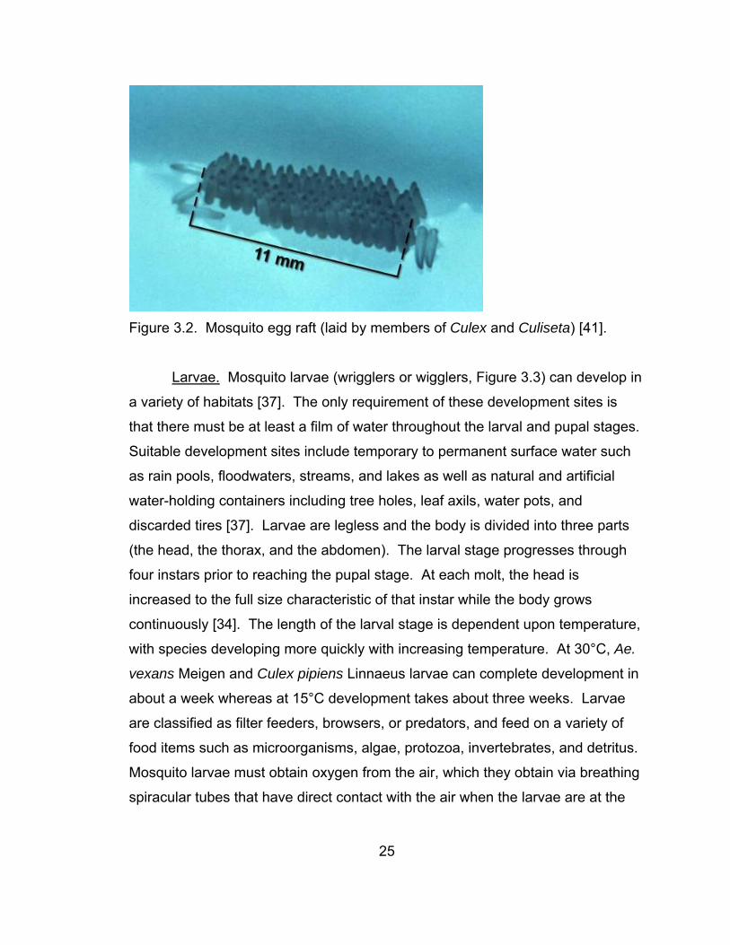
Figure 3.2. Mosquito egg raft (laid by members of Culex and Culiseta) [41].
Larvae. Mosquito larvae (wrigglers or wigglers, Figure 3.3) can develop in
a variety of habitats [37]. The only requirement of these development sites is
that there must be at least a film of water throughout the larval and pupal stages.
Suitable development sites include temporary to permanent surface water such
as rain pools, floodwaters, streams, and lakes as well as natural and artificial
water-holding containers including tree holes, leaf axils, water pots, and
discarded tires [37]. Larvae are legless and the body is divided into three parts
(the head, the thorax, and the abdomen). The larval stage progresses through
four instars prior to reaching the pupal stage. At each molt, the head is
increased to the full size characteristic of that instar while the body grows
continuously [34]. The length of the larval stage is dependent upon temperature,
with species developing more quickly with increasing temperature. At 30°C, Ae.
vexans Meigen and Culex pipiens Linnaeus larvae can complete development in
about a week whereas at 15°C development takes about three weeks. Larvae
are classified as filter feeders, browsers, or predators, and feed on a variety of
food items such as microorganisms, algae, protozoa, invertebrates, and detritus.
Mosquito larvae must obtain oxygen from the air, which they obtain via breathing
spiracular tubes that have direct contact with the air when the larvae are at the
25

water surface [34]. Because of this, larval control of mosquitoes is typically
accomplished using degradable oils that disrupt the surface tension of water and
penetrate the tracheal systems of larvae, resulting in suffocation [37].
Figure 3.3. Mosquito larvae [41].
Pupae. Mosquito pupae (tumblers, Figure 3.4) are comma-shaped [37].
The pupal stage is very short, lasting only about two days, during which
metamorphosis takes place and larval features are lost as the body of the adult
takes form [34]. The body of a pupa consists of a cephalothorax (fused head and
thorax) and the abdomen. The cephalothorax also has a pair of respiratory
trumpets that provide the developing adult with oxygen. Pupae are quite mobile
but they do not feed. Pupae are also resistant to desiccation, and adults can
emerge even if breeding sites have almost dried out [34].
26

Figure 3.4. Mosquito pupae [41].
Adults. Adult mosquitoes emerge from the pupal stage at the water
surface by increasing their hydrostatic pressure, causing the cuticle of the pupa
to split. The legs and wings are stretched as the mosquito increases the
hemolymph pressure, and the soft tissue becomes sclerotized within a few
minutes, allowing the mosquito to fly [34]. The adult body (Figure 3.5) consists of
a head, thorax, and abdomen. The body of the mosquito is typically covered with
patterns of scales, setae, and fine pile that are characteristics that aid in species
identification [37]. At emergence, male mosquitoes are not sexually mature; they
emerge a few days earlier than the females and thus reach sexual maturity at the
same time, which synchronizes mating compatibility [34].
27

Figure 3.5. Anatomy of the adult mosquito [41].
In mosquitoes, mating occurs when a female enters a lek (swarm of
males) [34]. In these swarms, males exhibit a flying behavior known as “dancing
flight” in which the males fly forward and backward and up and down over an
object (swarm marker) that contrasts with the surroundings. When the female
enters the swarm, she is seized by a male and they copulate face to face while
flying outside the swarm. The female only mates once and stores sperm to
fertilize future eggs whereas the male may mate with multiple females [34].
Although some mosquitoes are autogenous and eggs can develop without
a blood meal, most female mosquitoes are anautogenous and must take a blood
meal from a host animal to acquire adequate protein for the eggs to complete
oogenesis [37]. Female mosquitoes locate potential blood meal hosts through
sensory cues such as olfactory, visual, and thermal stimuli, with host odors
detected by antennal receptors [34]. Female mosquitoes are attracted to carbon
dioxide, lactic acid, octenol, acetone, butanone, and phenolic compounds. The
first phase of host location involves non-orientated flight in which the mosquito
flies upwind in a random motion in search of any of the above stimuli. When a
28

stimulus is detected, the flight behavior is changed and oriented towards the
host’s location. The mosquito flies upwind in a zig-zag pattern that holds the
mosquito in the stimulus plume and brings it closer to the source of the stimulus.
As the mosquito nears the host, it uses visual contact to locate the host and
compound eyes discriminate between form, movement, light contrast, and color
[34].
Once the female mosquito locates the host, the female probes the skin
several times with her proboscis, using temperature and thickness of the skin as
stimuli, in order to find a capillary [34]. The mosquito’s proboscis contains the
mouthparts, which include the labrum, paired mandibles, hypopharynx, paired
maxillae, and labium (Figure 3.6). All but the labium have evolved into hardened,
fine stylets that form a tightly fitting fascicle that penetrates the host’s skin, with
the labium serving as a sheath to enclose these mouthparts [37].
Figure 3.6. Mouthparts of the female adult mosquito. Modified from Service [42].
When feeding, the fascicle of stylets penetrates the skin as the labium is
bent backward at the skin surface [37]. The mandibles and maxillae move
29

alongside each other in a quick, stabbing motion that causes the tissue to be
gripped by the maxillary teeth, allowing the stylets to penetrate epidermal and
subepidermal tissue. The end of the fascicle is flexible and may bend at sharp
angles, to allow the mosquito to search in various directions throughout the
subepidermal tissue for small arterioles or venules. The hypopharynx releases
saliva that contains apyrase, an antihemostatic enzyme that inhibits platelet
aggregation and allows blood to flow freely from punctured vessels, and
anticoagulants, which prevent the blood from clotting. Together, these aid the
mosquito in finding a blood vessel, shortening the time required for feeding on a
host [37]. After finding a vessel, the fascicle is inserted into the lumen of the
vessel and blood is ingested up the food canal using the cibarium and
pharyngeal pumps, is transported through the esophagus, and accumulates in
the midgut. Stretch receptors in the abdomen signal the mosquito that there is
sufficient blood in the midgut, and she uses her forelegs to remove the fascicle
from the skin. When the female mosquito is fully engorged with blood, she is
unable to fly long distances and will seek a suitable resting site in which to digest
the blood meal and allow for egg development [37]. Oviposition occurs two to
four days (or longer depending upon the temperature) after ingestion of a blood
meal. Mosquitoes can lay between 50 to 500 eggs, and development of the eggs
continues as previously described [34].
Hibernation. In tropical areas, mosquitoes are active year-round because
suitable environmental conditions and habitats exist for larval development. In
temperate areas, however, winter conditions are much harsher and therefore
mosquitoes enter a period of dormancy [37]. Mosquitoes are capable of
hibernation at various stages of development, and the life stage that becomes
dormant is based upon the length and severity of the region’s dry season or
winter and also upon the mosquito species. Aedes spp., Psorophora spp., and
Ochlerotatus spp. all have quiescent eggs and hibernation occurs in the egg
stage [37]. In other species, hibernation occurs in the third or fourth larval instar
30
and these are capable of surviving in breeding sites that do not freeze or that
only have a frozen surface for a short time. Mosquitoes of Culex, Culiseta,
Uranotaenia, and Anopheles overwinter in the adult stage. These mosquitoes
enter a period of diapause and seek shelter in frost-free areas such as cellars
and burrows. Prior to hibernation, they feed intensively on plant juices in the
autumn and may also use the blood-fed body to synthesize lipid reserves during
diapause [34].
Mosquito Life History and Medical Importance
Of the 14 genera that are known to exist in North America north of Mexico
[36], at least seven (including 29 species) occur in the Lubbock, TX, area and
thus are the focus of this research.
Aedes. Eggs of Aedes spp. are always laid singly on damp areas just
above the waterline and are capable of withstanding desiccation [43]. After
flooding, some eggs hatch within a few minutes whereas others require
prolonged submersion or multiple soakings followed by short periods of
desiccation to induce development. Changes in day length, temperature, and
reduction in the oxygen content of the water are all environmental cues for the
development of eggs. Development of Aedes spp. can be rapid, occurring as
quickly as seven days, but typically takes 10 to 12 days to several weeks or
months. Generally, Aedes spp. feed during the day and early evening [43].
Members of this genus overwinter in the egg stage [44].
Aedes aegypti Linnaeus is commonly known as the yellow fever mosquito
because it is the major vector of the disease [45]. They typically occur in close
proximity to human dwellings and larvae are found in artificial containers such as
flower pots, water storage containers, broken bottles, and discarded tires,
typically within 500 m of the dwelling. Following heavy rainfall, larvae may also
be found in vegetation such as tree holes, leaf axils, and coconut shells. Larvae
are also known to be found in artificial and natural waters in harbors and on
31
ships. Eggs are laid close to the water line and are resistant to desiccation.
Optimal temperatures for development are 27 to 30°C and adults emerge within
10 days under these conditions. Aedes aegypti prefer to feed on human blood
(anthropophagous) and feeding occurs during the day in shady areas and
occasionally at night in lit rooms. They also rest indoors and do not migrate over
long distances [45]. In addition to yellow fever, Ae. aegypti also transmits
dengue [44].
Aedes albopictus Skuse, or the Asian tiger mosquito, is an exotic species
that has been introduced into many areas due to the worldwide trade in used
tires, including the introduction of the species into North America in Houston, TX,
in 1985 [37]. Larvae are found in small natural and artificial containers, and eggs
are resistant to desiccation. Females prefer to feed on humans but also may
feed on other mammals and some birds, and they tend to feed during dusk and
at night (readily entering houses to feed) but will also bite during the daytime [45].
Aedes albopictus is a vector of dengue, eastern equine encephalitis (EEE), and
dog heartworm [44].
Aedes cinereus Meigen eggs are laid in areas prone to flooding. Larvae
most often occur at the edges of semi-permanent, partly shaded pools of water
and at the edges of lakes with aquatic vegetation. Larvae begin to hatch at
temperatures of 12 to 13°C, and optimum conditions for development are 24 to
25°C in which larvae can develop in 8 to 10 days. Aedes cinereus are
crepuscular (feeding at dusk and dawn) and feed on mammals (zoophagous).
During the day, they rest in low vegetation out of sunlight [45]. The flight range of
Ae. cinereus appears to be limited in that they are only found in wooded areas
near larval habitats. Although they may be a pest species, they are not known to
transmit diseases [44].
Aedes vexans (inland floodwater mosquito, Figure 3.7) is a nuisance
mosquito because of the large numbers that hatch and emerge to seek blood
meals [45]. Aedes vexans is the most widespread of the Aedes spp. in the
32

United States and in many areas it is the most abundant and troublesome
mosquito [44]. They breed in floodplains of rivers or lakes with fluctuating water
levels and prefer sites with temporary bodies of fresh water. Aedes vexans
thrives in neutral to alkaline water occurring days to weeks following floods.
Larvae begin to eclose at temperatures of 9°C and hatching is adjusted to the
conditions of the temporary water. Aedes vexans undergo a process of “hatching
in installment” in which only a portion of the larvae undergo development [45]. If
those fail to complete development due to drying out, a second population can
begin development following a flood, without additional eggs being laid. Eggs
are also capable of surviving for at least five years if suitable hatching conditions
fail to exist. With high water temperatures, hatching rate is high and Ae. vexans
is often the dominant species during summer months with heavy rainfall.
Because of the high numbers of larvae that can occur in a single area, females
often migrate long distances (15 km) in search of a blood meal. Aedes vexans
prefer to feed on mammals, including humans. With optimum conditions, time
from hatching of one generation to hatching of the next generation is less than
three weeks [45]. Adults typically feed at dusk and after dark and rest during the
day in vegetation. Aedes vexans are vectors of St. Louis encephalitis (SLE),
EEE, western equine encephalitis (WEE), and LaCrosse encephalitis [44].
33
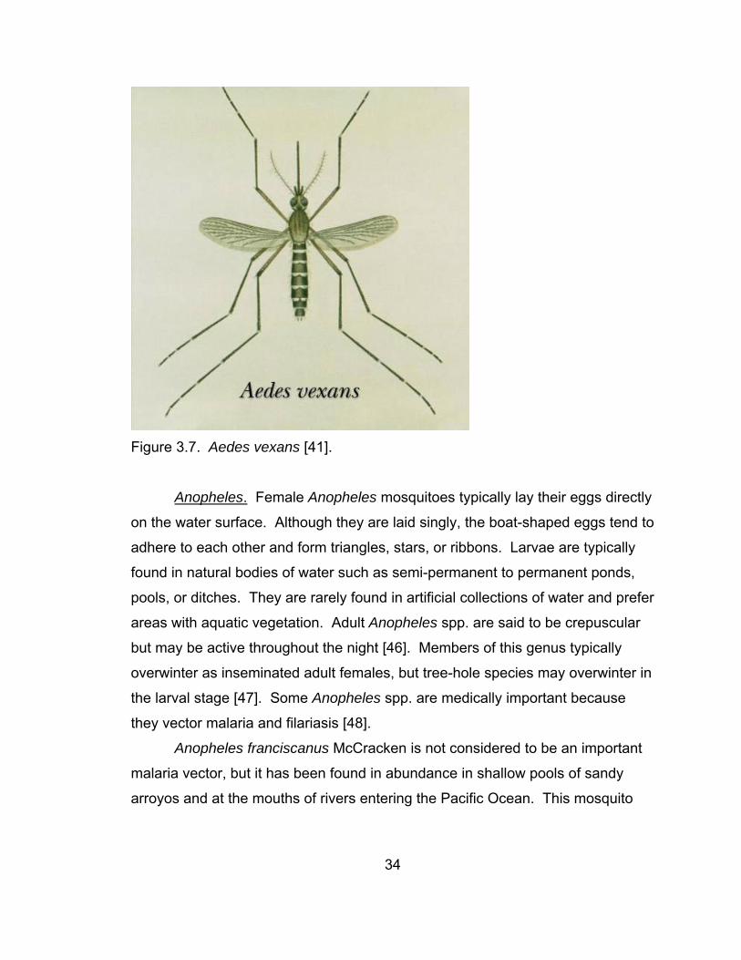
Figure 3.7. Aedes vexans [41].
Anopheles. Female Anopheles mosquitoes typically lay their eggs directly
on the water surface. Although they are laid singly, the boat-shaped eggs tend to
adhere to each other and form triangles, stars, or ribbons. Larvae are typically
found in natural bodies of water such as semi-permanent to permanent ponds,
pools, or ditches. They are rarely found in artificial collections of water and prefer
areas with aquatic vegetation. Adult Anopheles spp. are said to be crepuscular
but may be active throughout the night [46]. Members of this genus typically
overwinter as inseminated adult females, but tree-hole species may overwinter in
the larval stage [47]. Some Anopheles spp. are medically important because
they vector malaria and filariasis [48].
Anopheles franciscanus McCracken is not considered to be an important
malaria vector, but it has been found in abundance in shallow pools of sandy
arroyos and at the mouths of rivers entering the Pacific Ocean. This mosquito
34
has similar habits as An. pseudopunctipennis Theobald [44]. Anopheles
pseudopunctipennis prefers sunlit aquatic habitats with algae, such as at edges
of streams and seepage waters. They are indiscriminate feeders, feeding both
indoors and outdoors and on both humans and domestic animals [46]. In the
foothill regions of Mexico, An. pseudopunctipennis is an important vector of
malaria [44].
Anopheles punctipennis Say is the first of the Anopheles spp. to appear in
the spring and larvae are found in a variety of aquatic habitats. Larvae are found
in permanent pools, temporary water collections, and along margins of streams.
This species is not a natural vector of malaria [44].
Anopheles quadrimaculatus Say is known as the common malaria
mosquito and was the most important malaria vector in the United States, as it
was involved in almost all the human malaria cases that occurred east of the
Rocky Mountains [44]. Larvae are typically found in freshwater containing
vegetation or floating debris and are most abundant in shallow water. This
species has been found in both open, sunlit waters as well as densely shaded
swamps, although they show a preference for clear, quiet waters. Optimal
temperature for larval development is approximately 30°C, at which larvae
develop within two weeks. Adults feed at night and rest in cool, damp, dark
places during the daytime. Anopheles quadrimaculatus are zoophagous and
feed primarily on horses, cows, pigs, and chickens, but will also feed on human
hosts. Although production can continue throughout the year in warm areas, in
most of their range, fertilized adult females hibernate in protected areas such as
in caves or basements. In the spring, these females emerge, take a blood meal,
and then deposit their eggs. Each season, there may be nine or ten generations
produced, with populations peaking around July and August and declining in
September and October [44].
Culex. Culex spp. eggs are laid upright on the water surface and form an
egg raft of about 300 eggs. These eggs are oviposited in containers such as
35

cans and ground collections of water such as ditches and pools. Some species
also lay eggs in tree holes and leaf axils [43]. Culex spp. overwinter as
inseminated diapausing females. They are vectors of a number of arboviruses
and avian malaria. They generally feed on birds but may take a blood meal from
other animals as well [47].
Culex quinquefasciatus Say, or the southern house mosquito, is one of the
most important species in medical entomology [43]. It develops in stagnant pools
of water polluted with organic debris (rotting vegetation, household waste, or
excreta) such as in partially blocked drainage ditches and septic tanks. The
mosquito thrives in urban areas with poor drainage and sanitation, where its
populations may increase rapidly. Culex quinquefasciatus typically feeds at night
and rest indoors before and after feeding [43]. Culex quinquefasicatus is an
important vector in urban SLE epidemics, avian malaria, human filarial worm, dog
heartworm, and WEE [47].
Culex restuans Theobald larvae develop in pools of polluted water
containing decaying grass and leaves. Culex salinarius Coquillett larvae are
typically found in grassy pools of fresh and brackish waters. They commonly
appear at margins of lakes and cattail bogs [44]. Culex erthrothorax Dyar is
another member of this genus found in the Lubbock area.
Culex tarsalis Coquillett (Figure 3.8) thrive in sunny collections of
terrestrial water such as in ditches and in corrals [47]. In arid to semi-arid
regions, larvae are commonly found in temporary to semi-permanent bodies of
water associated with irrigation, including ditches and hoof prints, as well as in
artificial containers. Adults are crepuscular and rest in sheltered areas during the
day such as in vegetation, animal burrows, and on shaded sides of buildings.
Culex tarsalis have a feeding preference for birds (ornithophagous) but also feed
on cows, horses, and humans. They are the most important vectors of
encephalitis to man and horses in the western states and have been found to
vector both SLE and WEE [44].
36

Figure 3.8. Culex tarsalis [41].
Culiseta. Female Culiseta spp. lay egg rafts similar to those of Culex spp.
[47] and have similar habits as Culex spp. Culiseta mosquitoes are generally
unimportant as pest species [44]. In some areas, they overwinter as larvae [47],
but in warmer environments they are active throughout the winter [44].
Culiseta inornata Williston breed throughout the spring and summer in
northern and western states, but in the southern states they breed during the
winter as well. Larvae are typically found in cold water. They typically feed on
domestic animals and rarely bite humans. Culiseta inornata has been found to
be infected with Jamestown Canyon virus [44] and is involved in the transmission
of WEE and EEE [47].
Ochlerotatus. Once a subgenus of Aedes, Ochlerotatus was promoted to
genus rank in 2000 [49]. Recently there has been considerable discussion
concerning the validity of this generic status, with taxonomists arguing that
37
Ochlerotatus should be returned to the subgeneric level in Aedes [39]. However,
during the course of this research, Ochlerotatus was the accepted genus name
and thus species in this group are referred to as members of Ochlerotatus.
Ochlerotatus spp. habits and life histories resemble those of Aedes spp. [34].
Ochlerotatus atlanticus Dyar and Knab larvae are typically found in
flooded woodland bottoms or temporary pools in or near woods. Ochlerotatus
stimulans Walker is one of the most annoying and abundant woodland
mosquitoes and readily attacks during the daytime [44]. Ochlerotatus thelcter
Dyar and Oc. zoosophus Dyar and Knab are other members of this genus found
in the Lubbock area.
Ochlerotatus dorsalis Meigen readily feed on humans and inflict painful
bites. Larvae are found in small, open bodies of water and swamps and in
temporary to permanent waters formed by rainfall or melted snow, such as inland
pastures and drainage ditches. Females primarily feed in the late afternoon and
early evening hours, but feeding may continue throughout the night and during
the day in open areas [45]. Ochlerotatus dorsalis is a major pest species to both
humans and livestock in arid and semi-arid regions. This species is also known
to vector WEE [44].
Ochlerotatus nigromaculis Ludlow is associated with irrigated pastures,
especially in California. Their development is very rapid, with adults emerging as
quickly as four days from time of oviposition, and swarms have been known to
affect the behavior of livestock [47]. Ochlerotatus nigromaculis is known to
transmit WEE, California encephalitis, and SLE [44].
Ochlerotatus punctor Kirby larvae hatch during snow-melt and prefer
swampy forests with boggy water. The optimal temperature for development is
25°C, at which adults emerge at 10 to 17 days; however, the lowest mortality
rates are found at 15°C. Mortality of larvae occurs at temperatures at or above
30°C. Although they primarily feed at dusk, they may also feed during the day in
shaded areas [45].
38
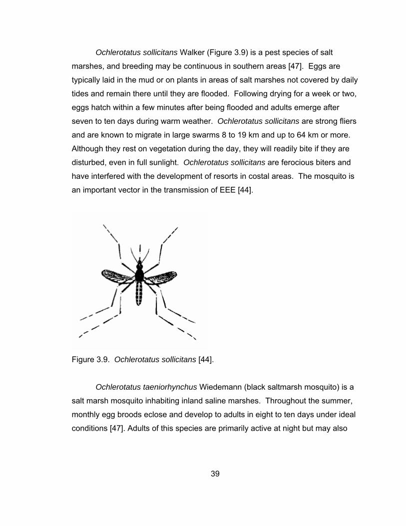
Ochlerotatus sollicitans Walker (Figure 3.9) is a pest species of salt
marshes, and breeding may be continuous in southern areas [47]. Eggs are
typically laid in the mud or on plants in areas of salt marshes not covered by daily
tides and remain there until they are flooded. Following drying for a week or two,
eggs hatch within a few minutes after being flooded and adults emerge after
seven to ten days during warm weather. Ochlerotatus sollicitans are strong fliers
and are known to migrate in large swarms 8 to 19 km and up to 64 km or more.
Although they rest on vegetation during the day, they will readily bite if they are
disturbed, even in full sunlight. Ochlerotatus sollicitans are ferocious biters and
have interfered with the development of resorts in costal areas. The mosquito is
an important vector in the transmission of EEE [44].
Figure 3.9. Ochlerotatus sollicitans [44].
Ochlerotatus taeniorhynchus Wiedemann (black saltmarsh mosquito) is a
salt marsh mosquito inhabiting inland saline marshes. Throughout the summer,
monthly egg broods eclose and develop to adults in eight to ten days under ideal
conditions [47]. Adults of this species are primarily active at night but may also
39

attack during the day in shady areas. Ochlerotatus taeniorhynchus is a vector of
dog heartworm [44].
Ochlerotatus triseriatus Say, or the Eastern treehole mosquito, larvae
develop in tree holes and artificial containers such as tires, cans, and barrels.
Larval development is slow, taking up to a month to complete. Adults feed during
the day in wooded areas and around tree holes where larvae develop.
Ochlerotatus triseriatus is a vector of LaCrosse encephalitis and dog heartworm
[44].
Psorophora. Although Psorophora spp. are typically not medically
important, they are vicious biters and adults can be very large. They are similar
to Aedes spp. in that their eggs can withstand desiccation and breeding areas
often consist of flooded pastures. They are only found in the Americas from
Canada to South America [43]. Psorophora spp. habits and life histories
resemble that of Aedes spp. [47].
Psorophora ciliata Fabricius is a large mosquito that is commonly known
as the gallinipper [44]. These mosquitoes feed during the day and night.
Psorophora ciliata larvae are predatory and one of the few species that feeds on
other aquatic insects, including other mosquito larvae. These larvae are often
found in temporary pools, sometimes in association with Ae. vexans, on which
they feed [44].
Psorophora columbiae Dyar and Knab is a fierce biter and commonly
breeds in rice fields. These mosquitoes were responsible for a reduction in the
milk supply during a four-day infestation in 1932 in the Everglades region of
Florida as well as great loss of livestock [47]. This species was also partially
responsible for the outbreak of Venezuelan equine encephalitis (VEE) in Texas in
1971. Psorophora columbiae feed anytime during the day or night, and large
populations of these make it unbearable for humans to remain outdoors, as well
as cause occasional livestock deaths. Eggs are laid on the soil in areas subject
to flooding, and larvae develop in temporary rain pools and irrigation waters.
40

These mosquitoes have been known to transmit WEE and California encephalitis
[44].
Psorophora cyanescens Coquillett was a bothersome pest following the
floods in 1967 in the Rio Grande Valley of Texas [44]. Psorophora cyanescens
are similar to Ps. columbiae in that they breed in temporary pools and are vicious
biters that feed during the day and night. This species can also become quite
abundant following rains in July and August [44].
Psorophora signipennis Coquillett larvae can develop and adults can
emerge in five days under favorable conditions. Larvae are typically found in
temporary ground pools. LaCrosse encephalitis and WEE have both been
isolated from Ps. signipennis [44].
Uranotaenia. Larvae of these mosquitoes are typically found in grassy
margins of lakes and ground collections of water. They have also been found in
tree holes and pot holes [44]. Uranotaenia spp. generally overwinter as adults
[34]. The only member of this genus collected in the Lubbock area is
Uranotaenia sapphirina Osten Sacken.
Mosquito Collection Methods
Many different mosquito collection methods have been developed over
time to estimate the number and relative abundance of species occurring in a
given area. Because only female mosquitoes blood feed, they are of most
concern in vector-borne disease surveillance. Trapping methods have been
developed based upon the stimuli female mosquitoes use for locating a host for
blood feeding. Some of these trapping methods are briefly discussed here. For
a more in-depth discussion of these trapping methods, refer to Mosquito Ecology:
Field Sampling Methods by M.W. Service [50].
Carbon Dioxide Traps. It has long been known that mosquitoes are
attracted to carbon dioxide and that carbon dioxide produced by breathing is one
of the key stimuli in attracting mosquitoes to a host [51]. The use of carbon
41
dioxide traps can be as simple as baiting a bed net then tucking up one or more
sides. Carbon dioxide used with light traps has been shown to increase the
number of mosquitoes collected as well as altering the species composition of
the collection [51]. Since the 1970s, the use of carbon dioxide in conjunction with
light traps has increased. The light source has also been removed in these traps
so that carbon dioxide is the only stimulus because studies have shown an
increase in mosquito catches without the light source for some species. This
increased effectiveness could be due to a more efficient fan because of the
decreased drain on the battery that typically operates both the light source and
the fan, but this has not yet been proven [51]. For mosquito collection, carbon
dioxide in the form of gas or Dry Ice® may be used. Although carbon dioxide gas
allows for greater control of the rate of carbon dioxide discharge, Dry Ice® is
usually less costly and more convenient but may have the adverse effects of
lowering the temperature in the area of the trap or greatly increasing the level of
carbon dioxide and actually deterring mosquitoes from the trap. Examples of
carbon dioxide traps include human-bait catches, malaise traps, and light traps
baited with carbon dioxide (Figure 3.10) [51].
42

Figure 3.10. Dry Ice® baited light trap set by Texas Tech University.
Light Traps. Insects have long been collected using light traps, the
earliest of which used paraffin or acetylene lamps as a light source [51]. Many
insects are strongly attracted to light sources whereas others seem to be
disoriented by light. These insects, including mosquitoes, may display positive
phototaxis and then negative phototaxis at varying intensities of light.
Mosquitoes are repelled by bright lights, so a fan is used in the trap to draw down
the mosquitoes that typically would fly around the light source but not enter the
trap. In addition, not all species of mosquitoes are attracted to light traps, and
collections from light traps may be disproportionate to the actual size of the
population and community composition. Light traps are also ineffective in
collecting day-flying mosquitoes [51].
Light traps have been typically used to determine changes in abundance
before and after mosquito control campaigns, annual and seasonal fluctuations in
community numbers, and in mosquito population and dispersion studies [51].
Examples of light traps include the Standard New Jersey light trap and the
43

Centers for Disease Control and Prevention (CDC) ultraviolet light trap (Figure
3.11), as well as the encephalitis virus surveillance (EVS) light trap (Figure 3.10
above), which is typically baited with Dry Ice® in addition to the light stimulus [51].
Figure 3.11. New Jersey light trap (left) set by the City of Lubbock and CDC
ultraviolet light trap (right) set by Texas Tech University.
Visual Attraction Traps. In these traps it has been found that the
percentage of luminous reflectance of light was inversely proportional to the
numbers of mosquitoes collected [51]. These traps are not widely used in
mosquito collections but have been used when baited with Dry Ice®. Primarily,
these traps have been used as a control method for tsetse flies because they are
so effective in collecting this fly. Examples of visual attraction traps include the
Haufe and Burgess trap, the Fay-Prince trap, the Wilton and Kloter cylinder trap,
and the duplex cone trap [51].
Sound Traps. Male mosquitoes have been shown to be attracted to a
recording of the sound of the female wingbeat as well as to the sound of a tuning
44

fork [51]. Other studies have shown that mosquitoes that feed on frogs are
attracted to frog noises emitted from a cassette player. Since these traps only
attract males within a short distance, they are often used in conjunction with a
swarm marker to bring males into the effective distance of a sound trap.
Examples of these traps include Ikeshoji cylinder sound traps, Ikeshoji and
Ogawa cup traps, and Kanda et al. cylinder and lantern traps [51].
Egg and Larval Mosquito Collections. Mosquito community abundance
can also be determined based upon egg and larval surveillance [52]. The
collection of mosquito eggs is useful in determining the density of eggs in natural
habitats and in further understanding oviposition sites of various mosquito
species. Additionally, egg collections can be used as a basis for predicting future
larval populations and where mosquito control should be focused. Larval
collections are useful in assessing the aquatic stages of mosquitoes and in
determining mosquito community dynamics. They can also be used to estimate
population densities before and after larvicide application. Larvae are typically
collected using a dipper (Figure 3.12). Eggs of Anopheles, Culex, Uranotaenia,
Coquillettidia, and Culiseta can be collected using a modified dipper with the
bottom removed and replaced with fine wire mesh or by using pipets or small
nets. Soil samples must be taken for collection of Aedes and Ochlerotatus eggs
[52].
45

Figure 3.12. Dipper for the collection of mosquito larvae [41].
Research Goals and Hypotheses
The objective of this portion of the research project was to evaluate
environmental influences on mosquito community dynamics and to determine
seasonally-influenced changes in mosquito communities. The presence of
mosquito species and their abundances over time was correlated to weather
variables, including precipitation, relative humidity, air temperature, weekly heat
units, and cumulative heat units. Differences in mosquito communities between
collection locations were also determined based upon the characteristics of the
mosquito collection sites. Characterization of trapping sites included land use
and determination of vegetation density and potential resting areas, and
identification of external light sources, potential hosts, and potential breeding
areas. Determining the effect of environmental influences (including both
weather and trapping site profiles) in shaping mosquito community dynamics will
aid in developing a model for determining when and where mosquito control
operations should be undertaken. It is hypothesized that weather conditions,
especially rainfall, in the weeks prior to mosquito collection will have an influence
upon both the total number of mosquitoes collected as well as the community
structure of mosquito collections.
46

Materials and Methods
Mosquito Collection and Identification
Mosquitoes were collected throughout Lubbock County, TX (33.65°N;
101.81°W; 975 m elevation) from 2002 through 2004. Mosquitoes were collected
using multiple trapping locations and several different trap types to ensure
collection of a representative sample of the mosquito community occurring in the
area. Collected mosquitoes were returned to the lab and euthanized by placing
in a freezer (-20°C or -80°C) for at least 20 minutes. Mosquitoes were stored in
the freezer until processed. Mosquitoes were identified to species according to
Darsie and Ward [53] and the number of each species was counted and
recorded. Female mosquitoes were pooled into groups of no more than 50 per
species per site per week and stored in a -80°C freezer pending West Nile virus
(WNV) screening (Chapter IV). Turell and others [54] found that holding
temperature did not adversely affect the ability to detect WNV RNA (ribonucleic
acid); therefore, mosquito pools were held at -80°C until analysis.
Mosquito Collection Sites. Mosquito trapping sites were evaluated and
selected based upon observed or potential mosquito activity, access to the
potential trapping site (typically private property), and risk of trap vandalism or
theft. All trapping sites were characterized based upon their geographic location
and by their physical location and land use. Precise, geographically-referenced
locations for trapping sites were determined using Global Positioning System
(GPS) technologies from a Trimble GeoExplorer IITM (Trimble Navigation, Ltd.,
Sunnyvale, CA). The GPS locations were displayed on a digital orthographic
quadrangle map using MapInfo Professional® (MapInfo Corp., Troy, NY)
Geographic Information Systems software was used for graphical representation
of the trapping locations. Characteristics of each site deemed to be important in
their influence on mosquito collections included density of vegetation, proximity
to potential breeding sites, external light sources, and potential hosts, and these
47

features were determined qualitatively at each trapping location. Traps were set
consistently at trapping sites described in Appendix A for mosquito collection
during the study.
Mosquito Control Operations. Mosquito control operations by the City of
Lubbock were ongoing throughout this study. These typically involved the use of
ultra-low volume application of permethrin in the form of Permanone® (Bayer,
Montvale, NJ), but a variety of larvicides such as Altosid® (Wellmark
International, Bensenville, IL), VectoBac® (Valent BioSciences Corporation,
Libertyville, IL), and Golden Bear® (Clarke Mosquito Control, Roselle, IL) were
also used. Based upon spraying records obtained from the City of Lubbock, it
was difficult to determine whether these efforts may have affected mosquito
populations at trapping locations used throughout this study, because data
recording was not consistent over time nor among mosquito control operators.
However, since most of the mosquito collection sites were located within the city
limits and the City of Lubbock typically sprayed the entire city over a time period
of several weeks (personal communication, Joe Vargas, City of Lubbock), effects
of mosquito control at individual collection locations were assumed to be
negligible.
Encephalitis Virus Surveillance Light Traps and Centers for Disease
Control and Prevention Ultraviolet Light Traps. Mosquito surveillance operations
using EVS light traps (BioQuip Products, Rancho Dominguez, CA) baited with
Dry Ice® (Ace Dry Ice®, Lubbock, TX) were initiated in July 2002. Surveillance
efforts were intensified in 2003, with trapping operations conducted at least once
per week from April through early December, typically with two nights of trapping
conducted each week during the summer months. In 2003 there were seven
fixed trap sites with additional trap sites added as deemed necessary based
upon weather conditions, increased mosquito activity, and the presence of dead
birds. Surveillance was continued in 2004 with traps set at seven fixed locations
(some of which were not previous trapping locations) from February through mid-
48
November. Traps were set at least once each week and typically twice per week
during the summer months. Again, additional trap sites were added as deemed
necessary. Mosquitoes were collected using CDC light traps (BioQuip Products,
Rancho Dominguez, CA) equipped with an ultraviolet light only during 2004 at
four of the fixed EVS light trap sites. These traps were set at the same time as
the EVS traps but were separated from each other by at least 15 m to avoid
interference between the two types of stimuli.
New Jersey Light Traps. Mosquitoes collected using New Jersey light
traps (BioQuip Products, Rancho Dominguez, CA) were obtained from the City of
Lubbock during 2002, 2003, and 2004. The City of Lubbock utilized 25 fixed
sites at which New Jersey light traps were set and operated continuously for
seven days, with mosquitoes collected once per week from March through
November. During the winter months, traps were set at six fixed sites and
mosquito specimens were recovered each week. Mosquitoes were identified to
species by the city entomologist, and data sheets reflecting the collections for
each week and a sample of the collected mosquitoes were obtained from the City
of Lubbock. In order to compare mosquito collections using New Jersey light
traps, in which mosquitoes were collected over a seven-day period (seven trap-
nights per trap site), with data collected using ultraviolet and EVS light traps, in
which mosquitoes were collected during a one night period (one trap-night per
trap site), data regarding collections from New Jersey light traps were
standardized by determining the number of mosquitoes collected per trap-night.
In this standardization, the total number of mosquitoes collected in each trap was
divided by the number of nights the trap was operated.
Weather Data
Data collected for weather conditions were recorded as described in
Chapter II. Daily weather conditions were obtained from the United States
Department of Agriculture, Agricultural Research Service. Weekly averages for
49
air temperature and relative humidity and weekly totals for precipitation and heat
units were used to create a series of weather lags to determine the effects of the
previous week(s)’ weather on mosquito populations. See Appendix B for an
explanation of the weather lags evaluated.
Analyses
Smoothing spline transformations (smoothing parameter = 50) were
performed on mosquito collection data in order to remove “noise” in the data set
and obtain a curve of the general mosquito collection patterns. In addition,
smoothing spline transformations for weather data from Chapter II, as well as
weekly weather summaries and weather lags, were used to determine the effect
of weather conditions on mosquito communities. Regression was used to model
changes in weather over time and to evaluate any influences these changes had
upon mosquito communities. Differences in mosquito populations between
collection locations were determined using analysis of variance and Tukey’s
multiple comparison test. For these analyses, the total number of mosquitoes
collected per trap-night (y) using carbon dioxide baited light traps at the fixed
trapping locations was transformed by taking the natural logarithm of y+1 [ln
(y+1)]. All analyses were conducted using SAS version 9.1 (SAS Institute, Inc.,
Cary, NC) and graphical displays were produced using SigmaPlot version 2000
(Systat Software Inc., Richmond, CA).
Results and Discussion
The goal of this portion of the research project was to determine
seasonally-influenced trends in mosquito populations and to correlate those
trends with weather patterns proceeding mosquito collection as well as profiles of
mosquito collection locations. Understanding aspects of mosquito vectors,
including their biology, ecology, and behavior, is vital for predicting, identifying,
and managing outbreaks of mosquito-borne diseases [55]. The development of
50

models to understand why mosquito population explosions occur is critical for
effective mosquito surveillance and control operations. Table 3.1 displays the
total number of mosquitoes collected per trap-night throughout the study period,
with a breakdown of the total number of mosquitoes that were collected using
New Jersey light traps and by using EVS and ultraviolet light traps. Figure 3.13
displays the percentage generic composition for the total number of mosquitoes
collected.
51
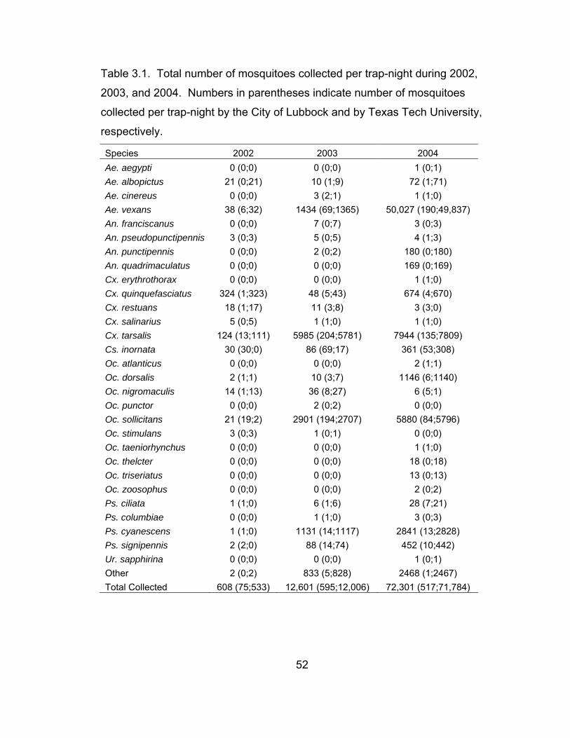
Table 3.1. Total number of mosquitoes collected per trap-night during 2002,
2003, and 2004. Numbers in parentheses indicate number of mosquitoes
collected per trap-night by the City of Lubbock and by Texas Tech University,
respectively.
Species 2002 2003 2004 Ae. aegypti 0 (0;0) 0 (0;0) 1 (0;1) Ae. albopictus 21 (0;21) 10 (1;9) 72 (1;71) Ae. cinereus 0 (0;0) 3 (2;1) 1 (1;0) Ae. vexans 38 (6;32) 1434 (69;1365) 50,027 (190;49,837) An. franciscanus 0 (0;0) 7 (0;7) 3 (0;3) An. pseudopunctipennis 3 (0;3) 5 (0;5) 4 (1;3) An. punctipennis 0 (0;0) 2 (0;2) 180 (0;180) An. quadrimaculatus 0 (0;0) 0 (0;0) 169 (0;169) Cx. erythrothorax 0 (0;0) 0 (0;0) 1 (1;0) Cx. quinquefasciatus 324 (1;323) 48 (5;43) 674 (4;670) Cx. restuans 18 (1;17) 11 (3;8) 3 (3;0) Cx. salinarius 5 (0;5) 1 (1;0) 1 (1;0) Cx. tarsalis 124 (13;111) 5985 (204;5781) 7944 (135;7809) Cs. inornata 30 (30;0) 86 (69;17) 361 (53;308) Oc. atlanticus 0 (0;0) 0 (0;0) 2 (1;1) Oc. dorsalis 2 (1;1) 10 (3;7) 1146 (6;1140) Oc. nigromaculis 14 (1;13) 36 (8;27) 6 (5;1) Oc. punctor 0 (0;0) 2 (0;2) 0 (0;0) Oc. sollicitans 21 (19;2) 2901 (194;2707) 5880 (84;5796) Oc. stimulans 3 (0;3) 1 (0;1) 0 (0;0) Oc. taeniorhynchus 0 (0;0) 0 (0;0) 1 (1;0) Oc. thelcter 0 (0;0) 0 (0;0) 18 (0;18) Oc. triseriatus 0 (0;0) 0 (0;0) 13 (0;13) Oc. zoosophus 0 (0;0) 0 (0;0) 2 (0;2) Ps. ciliata 1 (1;0) 6 (1;6) 28 (7;21) Ps. columbiae 0 (0;0) 1 (1;0) 3 (0;3) Ps. cyanescens 1 (1;0) 1131 (14;1117) 2841 (13;2828) Ps. signipennis 2 (2;0) 88 (14;74) 452 (10;442) Ur. sapphirina 0 (0;0) 0 (0;0) 1 (0;1) Other 2 (0;2) 833 (5;828) 2468 (1;2467) Total Collected 608 (75;533) 12,601 (595;12,006) 72,301 (517;71,784)
52

N=9816 N=40,608 N=92,923
12%
31%
14%
36%
7%
12%
40%
4%
34%
7%
62%
15%
2%12%
5%P
erce
ntag
e G
ener
ic C
ompo
sitio
n
N=9816 N=40,608 N=92,923
12%
31%
14%
36%
7%
12%
40%
4%
34%
7%
62%
15%
2%12%
5%
N=9816 N=40,608 N=92,923
12%
31%
14%
36%
7%
12%
40%
4%
34%
7%
62%
15%
2%12%
5%
N=9816 N=40,608 N=92,923
12%
31%
14%
36%
7%
12%
40%
4%
34%
7%
62%
15%
2%12%
5%P
erce
ntag
e G
ener
ic C
ompo
sitio
n
Figure 3.13. Percentage generic composition of total number of mosquitoes
collected each year, 2002 through 2004.
Historical records of mosquito collections throughout Texas indicate that of
the species known to occur in North America north of Mexico, over half of these
species have been collected in Texas [56]. Recent reports have indicated that
there are at least 86 species of mosquitoes that occur throughout Texas [57].
The reason for such diversity in mosquito populations is likely due to variation in
climate and geography in Texas. Climate in Texas ranges from humid to arid,
and the geography consists of beaches, wetlands, forests, deserts, grasslands,
and mountains. All of these factors allow for a large number of habitats in which
different species of mosquito may find their niche, based upon their life-history
requirements.
Records of the community structure of mosquitoes in the Lubbock, TX,
area have not been published since the 1970s [58]. Thus, an important aspect in
determining mosquito community dynamics in the area was to develop an
updated species checklist of mosquitoes of Lubbock, Texas. Historical
53

community structure in Lubbock, TX, consisted of Ae. vexans, Oc. nigromaculis,
Oc. dorsalis, Cx. tarsalis, Cx. erraticus Dyar and Knab, Cx. quinquefasciatus, Cx.
restuans, Cx. salinarius, Ps. ciliata, Ps. confinnis Lynch-Arribalzaga, Ps.
cyanescens, Ps. discolor Coquillett, Cs. incidens Thomson, Cs. inornata, An
pseudopunctipennis, An. punctipennis, and Ur. syntheta Dyar and Shannon [59].
Although some of these were not detected in a survey conducted in 1970,
additional species were found in the Lubbock area including Cx. erythrothorax,
Cx. peus Speiser, Ps. signipennis, and An. franciscanus [58]. Of these, Cx.
erraticus, Ps. confinnis, Ps. discolor, Cs. incidens, Ur. syntheta, and Cx. peus
were the only species that were not collected in this study; however, they may
still be present in the Lubbock area. In addition to these historical species, many
other species were collected in the Lubbock area. Distribution maps in Darsie
and Ward [53, 60] include many species of mosquitoes known to occur in this
region but not collected during the study period and exclude some that were
collected.
Also of interest is a comparison of the number of mosquitoes collected per
trap-night using New Jersey light traps compared to EVS and ultraviolet light
traps. Although direct comparisons are difficult as trapping procedure differed
between the City of Lubbock and Texas Tech University, obvious differences in
the number of mosquitoes collected per trap-night exist. The majority of the
mosquitoes collected by Texas Tech University were collected using EVS light
traps baited with Dry Ice®. As carbon dioxide is one of the chief stimuli
mosquitoes use in host-seeking, the increased number of mosquitoes collected
using carbon dioxide in addition to a light source compared to light alone is not a
surprise. Other studies have also shown an increase in mosquito collections
when light traps are baited with carbon dioxide [51].
As seen in Figure 3.13 above, the majority of the mosquitoes collected
were Aedes spp. (consisting primarily of Ae. vexans), Culex spp. (consisting
primarily of Cx. tarsalis), and Ochletotatus spp. (consisting primarily of Oc.
54

sollicitans). Because of this phenomenon, the remainder of the analyses on
mosquito collections were based upon these three species as well as the total
number of mosquitoes collected.
Differences in mosquito collections were apparent at the various trapping
locations. Mosquito collections using carbon dioxide baited light traps set at the
chicken coop (CC), Dub Parks Arena (DP), FOX television station (FOX),
Lubbock Christian University (LCU), Texas Tech Farm (ND), Reese Golf Course
(RSG), and Reese playground (RSP) were used for comparison of trapping
locations during the 2003 season whereas collections at DP, Texas Tech
Equestrian Center (EQ), FOX, KRFE radio station (KRFE), Meadowbrook Golf
Course (MBGC), RSP, and the Windmill Museum (WMM) were used during the
2004 season (Appendix A). During 2003, there was a significant difference in
mosquito collections between trapping sites in the total number of mosquitoes
collected (p<0.0001), the number of Ae. vexans collected (p=0.0307), the
number of Cx. tarsalis collected (p<0.0001), and the number of Oc. sollicitans
collected (p<0.0001) (Table 3.2). Analysis of variance indicated there was a
difference between trap sites in the number of Ae. vexans collected; however,
Tukey’s multiple comparison test did not detect these differences. In 2004, there
was a significant difference in mosquito collections between trapping sites in the
total number of mosquitoes collected, the number of Ae. vexans collected, the
number of Cx. tarsalis collected, and the number of Oc. sollicitans collected
(p<0.0001 for all) (Table 3.3).
55

Table 3.2. Differences between mosquito trap sites in total number of
mosquitoes collected, total number of Ae. vexans collected, total number of Cx.
tarsalis collected, and total number of Oc. sollicitans collected, 2003. Trapping
locations listed under each heading are significantly different, and locations
omitted or blank spaces indicate no significant difference (α=0.05).
Sites Total Ae. vexans Cx. tarsalis Oc. sollicitans
CC RSP, LCU, ND, DP RSP, DP, LCU RSP, DP, ND, LCU
DP CC, FOX, RSG CC, FOX CC
FOX DP DP, LCU
LCU CC CC, FOX CC, RSG
ND CC CC
RSG DP LCU
RSP CC CC CC
Table 3.3. Differences between mosquito trap sites in total number of
mosquitoes collected, total number of Ae. vexans collected, total number of Cx.
tarsalis collected, and total number of Oc. sollicitans collected, 2004. Trapping
locations listed under each heading are significantly different, and locations
omitted or blank spaces indicate no significant difference (α=0.05).
Sites Total Ae. vexans Cx. tarsalis Oc. sollicitans
DP KRFE, MBGC KRFE, MBGC KRFE, MBGC, FOX MBGC
EQ KRFE KRFE, MBGC KRFE, MBGC, FOX FOX, WMM, MBGC
FOX KRFE, MBGC RSP, EQ, DP EQ, MBGC
KRFE RSP, EQ, WMM, DP WMM, RSP, EQ,
FOX, DP
WMM, RSP, EQ, DP MBGC
MBGC WMM, DP WMM, RSP, EQ,
FOX, DP
WMM, RSP, EQ, DP EQ, RSP, DP,
KRFE, FOX
RSP KRFE KRFE, MBGC KRFE, MBGC, FOX MBGC
WMM KRFE, MBGC KRFE, MBGC KRFE, MBGC EQ
56

Because characteristics of trapping sites were not quantified and because
profiles of trapping sites change over time throughout the spring, summer, and
fall (in terms of water levels of playa lakes and standing water, density of
vegetation, likelihood of outdoor activity of potential hosts), explanation of the
differences in mosquito collections between trapping sites are difficult, but broad
conclusions can be drawn based upon subjective evaluation of the trapping sites.
Methods exist to analyze trapping sites based upon qualitative observations,
however, as the focus of this study was to determine influences of weather of
mosquito communities, these methods were not employed. In 2003, the majority
of the differences in trapping sites occurred between CC and the other trapping
locations. Differences between this site and DP and ND are likely due to
variations in the amount of vegetation present at CC and that the trap set at CC
was more protected from the wind. Subjective evaluation of vegetative biomass
at RSP and LCU was similar to CC, but large fields that collected runoff probably
allowed for more potential breeding sites at CC compared to RSP and LCU.
There were also more sources of external light at LCU than at CC. In 2004, most
of differences in mosquito collections occurred between KRFE and other
collection sites, and MBGC and other collection sites. Profiles of KRFE and
MBGC were very similar (based upon subjective evaluation of the trapping sites)
in that both had a high amount of organic debris as well as a high density of
vegetation. Differences in these trapping sites and other sites sampled were
likely due to the vegetation and organic debris as well as the availability of
potential breeding sites from standing water.
Other studies have shown that landscape characteristics influence
mosquito populations. In Buenos Aires, Argentina, vegetation cover (estimated
from digitized aerial photographs) was correlated to infestation of Ae. aegypti
larvae in water-filled containers in cemeteries [61]. Amount of vegetation and
habitat type were also critical factors in the collection of Cx. tarsalis in the
Coachella Valley of California. Mosquito abundance was much higher in areas
57
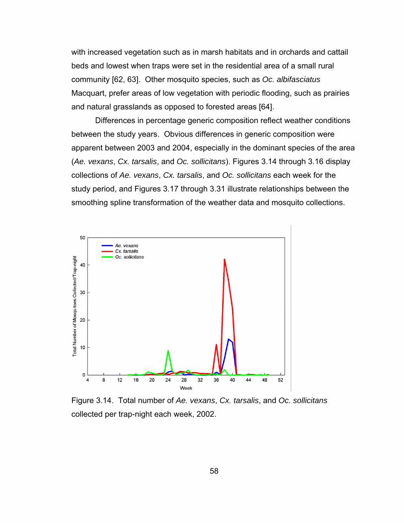
with increased vegetation such as in marsh habitats and in orchards and cattail
beds and lowest when traps were set in the residential area of a small rural
community [62, 63]. Other mosquito species, such as Oc. albifasciatus
Macquart, prefer areas of low vegetation with periodic flooding, such as prairies
and natural grasslands as opposed to forested areas [64].
Differences in percentage generic composition reflect weather conditions
between the study years. Obvious differences in generic composition were
apparent between 2003 and 2004, especially in the dominant species of the area
(Ae. vexans, Cx. tarsalis, and Oc. sollicitans). Figures 3.14 through 3.16 display
collections of Ae. vexans, Cx. tarsalis, and Oc. sollicitans each week for the
study period, and Figures 3.17 through 3.31 illustrate relationships between the
smoothing spline transformation of the weather data and mosquito collections.
Figure 3.14. Total number of Ae. vexans, Cx. tarsalis, and Oc. sollicitans
collected per trap-night each week, 2002.
58
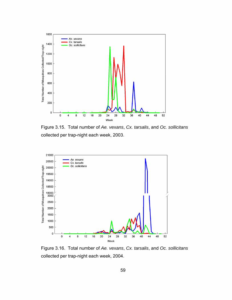
Figure 3.15. Total number of Ae. vexans, Cx. tarsalis, and Oc. sollicitans
collected per trap-night each week, 2003.
Figure 3.16. Total number of Ae. vexans, Cx. tarsalis, and Oc. sollicitans
collected per trap-night each week, 2004.
59
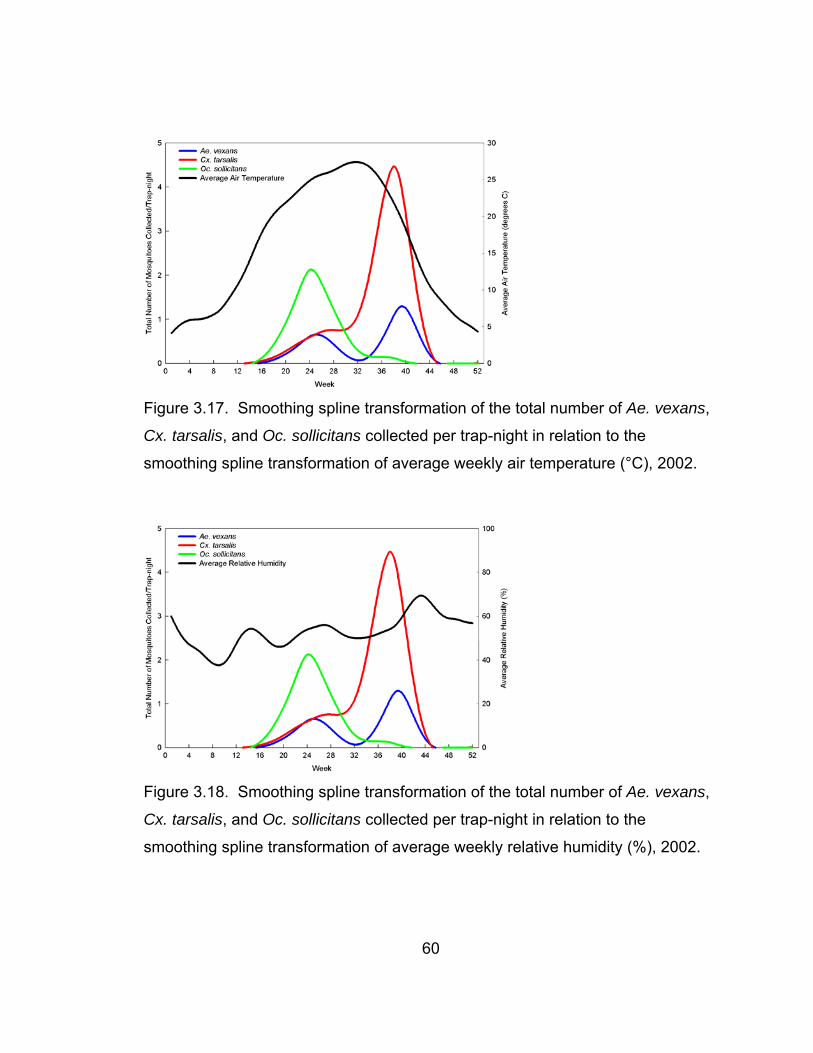
Figure 3.17. Smoothing spline transformation of the total number of Ae. vexans,
Cx. tarsalis, and Oc. sollicitans collected per trap-night in relation to the
smoothing spline transformation of average weekly air temperature (°C), 2002.
Figure 3.18. Smoothing spline transformation of the total number of Ae. vexans,
Cx. tarsalis, and Oc. sollicitans collected per trap-night in relation to the
smoothing spline transformation of average weekly relative humidity (%), 2002.
60

Figure 3.19. Smoothing spline transformation of the total number of Ae. vexans,
Cx. tarsalis, and Oc. sollicitans collected per trap-night in relation to total weekly
precipitation (mm), 2002.
Figure 3.20. Smoothing spline transformation of the total number of Ae. vexans,
Cx. tarsalis, and Oc. sollicitans collected per trap-night in relation to the
smoothing spline transformation of total weekly heat units, 2002.
61

Figure 3.21. Smoothing spline transformation of the total number of Ae. vexans,
Cx. tarsalis, and Oc. sollicitans collected per trap-night in relation to the
smoothing spline transformation of cumulative heat units, 2002.
Figure 3.22. Smoothing spline transformation of the total number of Ae. vexans,
Cx. tarsalis, and Oc. sollicitans collected per trap-night in relation to the
smoothing spline transformation of average weekly air temperature (°C), 2003.
62

Figure 3.23. Smoothing spline transformation of the total number of Ae. vexans,
Cx. tarsalis, and Oc. sollicitans collected per trap-night in relation to the
smoothing spline transformation of average weekly relative humidity (%), 2003.
Figure 3.24. Smoothing spline transformation of the total number of Ae. vexans,
Cx. tarsalis, and Oc. sollicitans collected per trap-night in relation to total weekly
precipitation (mm), 2003.
63

Figure 3.25. Smoothing spline transformation of the total number of Ae. vexans,
Cx. tarsalis, and Oc. sollicitans collected per trap-night in relation to the
smoothing spline transformation of total weekly heat units, 2003.
Figure 3.26. Smoothing spline transformation of the total number of Ae. vexans,
Cx. tarsalis, and Oc. sollicitans collected per trap-night in relation to the
smoothing spline transformation of cumulative heat units, 2003.
64

Figure 3.27. Smoothing spline transformation of the total number of Ae. vexans,
Cx. tarsalis, and Oc. sollicitans collected per trap-night in relation to the
smoothing spline transformation of average weekly air temperature (°C), 2004.
Figure 3.28. Smoothing spline transformation of the total number of Ae. vexans,
Cx. tarsalis, and Oc. sollicitans collected per trap-night in relation to the
smoothing spline transformation of average weekly relative humidity (%), 2004.
65
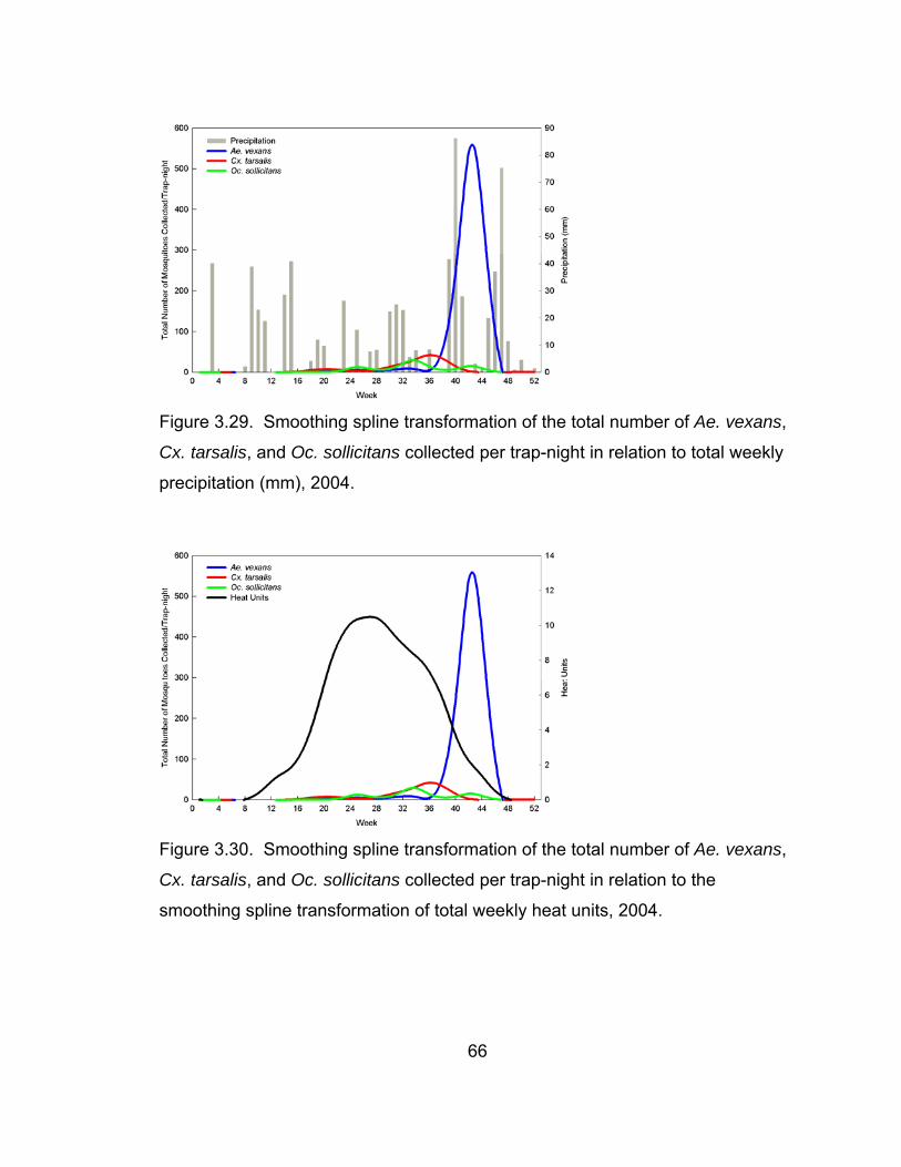
Figure 3.29. Smoothing spline transformation of the total number of Ae. vexans,
Cx. tarsalis, and Oc. sollicitans collected per trap-night in relation to total weekly
precipitation (mm), 2004.
Figure 3.30. Smoothing spline transformation of the total number of Ae. vexans,
Cx. tarsalis, and Oc. sollicitans collected per trap-night in relation to the
smoothing spline transformation of total weekly heat units, 2004.
66

Figure 3.31. Smoothing spline transformation of the total number of Ae. vexans,
Cx. tarsalis, and Oc. sollicitans collected per trap-night in relation to the
smoothing spline transformation of cumulative heat units, 2004.
High rains in a short time period during the spring of 2003 led to flooding
and the emergence of a large number of Oc. sollicitans (Figure 3.24). During
that summer, drought conditions persisted and Cx. tarsalis thrived in stagnant
pools, and rains in the fall led to an emergence of Ae. vexans. In 2004, however,
heavy rainfalls persisted throughout the spring, summer, and fall months,
resulting in a population explosion of Ae. vexans during the early fall months
(Figure 3.29). Peaks of Oc. sollicitans and Cx. tarsalis occurred during the
summer of 2004, and although there were increases in the numbers of these
mosquitoes collected compared to the previous year, the tremendous numbers of
Ae. vexans that fall dominated collections. Interesting to note also is that in all
three study years, Oc. sollicitans populations peaked around June and July, and
Ae. vexans populations peaked around October and November. Although the
Cx. tarsalis population peak was more variable, it always occurred between the
peaks of Oc. sollicitans and Ae. vexans.
67

Responses of these species to weather conditions are consistent with
their life histories. Culex tarsalis thrives in stagnant water bodies. The drought
conditions during the summer of 2003 provided ample habitats for the
proliferation of Cx. tarsalis and explained the dominance of that species that
year. In 2004, however, continuous rainfall likely flushed out suitable
development pools for Cx. tarsalis. On the other hand, Ae. vexans and Oc.
sollicitans are both floodwater mosquitoes and populations thrive in bodies of
fresh water, including those that occur a few days to weeks following rainfall. At
appropriate temperatures, populations of these species peak two to four weeks
following rainfall. This explains the peak of Oc. sollicitans seen several weeks
following rainfall during the spring of 2003. The high amount of rainfall
throughout 2004 explains the huge population of Ae. vexans in early fall, as eggs
were constantly flooded and carried to bodies of fresh water. Average weekly air
temperature, average weekly relative humidity, total weekly heat units, and yearly
cumulative heat units were roughly consistent over the three years, and
differences in mosquito collections based upon these weather parameters were
not apparent in graphical displays. Statistical analyses were able to detect more
latent patterns in these variables.
Regression analysis to produce models of mosquito occurrence in
response to weather conditions demonstrated that the total number of
mosquitoes collected per trap-night as well as the number of Ae. vexans, Cx.
tarsalis, and Oc. sollicitans collected per trap-night were highly dependent upon
weather conditions. Although the variables that explained mosquito occurrence
varied between years and among species, the best models usually consisted of a
lag term in the weather variable, indicating the weather conditions in the weeks
prior to collection influenced mosquito occurrence more than current weather
conditions. For this study, best models for mosquito community dynamics were
chosen by the maximum r2 improvement technique. This technique was chosen
because it does not settle on a single model, rather, it finds the best one-variable
68

model, the best two-variable model, and so on by adding or removing variables
which results in the largest increase in r2 for the model. Because a higher r2
value indicates a better fit of the model with the data, models with a higher r2
value were the best models for explaining the data obtained in this study.
As stated in Chapter II, 2002 was an average year for the Lubbock area
whereas 2003 was a drought year and 2004 was a wet year. The best one-
variable model of mosquito occurrence in 2002 was the total weekly heat units
four to eight weeks prior to collection (r2=0.5594, 0.4893, and 0.6707 for total
number of mosquitoes collected per trap-night, total number of Ae. vexans
collected per trap-night, and total number of Cx. tarsalis collected per trap-night,
respectively). The best two-variable models included the total amount of rainfall
three to eight weeks prior to collection, as well as the total heat units four to eight
weeks before collection (r2=0.6790, 0.5819, and 0.7401 for total number of
mosquitoes collected per trap-night, total number of Ae. vexans collected per
trap-night, and total number of Cx. tarsalis collected per trap-night, respectively).
See Tables 3.4 through 3.7 for complete model parameter estimates for the best
models containing one to five parameters for 2002.
69

Table 3.4. Best models relating total number of mosquitoes collected per trap-
night to weather conditions, 2002. All models were highly significant (p<0.0001). Model
r2
Variable Coefficient Standard
Error
p-value
0.5594 Intercept -0.96340 0.93703 0.3099
Total heat units, 4 to 8 wk prior to collection 0.02818 0.00391 < 0.0001
0.6790 Intercept 2.13047 1.13936 0.0688
Total heat units, 4 to 8 wk prior to collection 0.02644 0.00341 < 0.0001
Total rainfall, 4 to 8 wk prior to collection -0.05592 0.01449 0.0004
0.8613 Intercept -7.19380 1.72657 0.0002
Total heat units, 1 to 5 wk prior to collection 0.06708 0.00497 < 0.0001
Smoothing spline parameter, average air
temperature, week of collection
0.93411 0.17953 <0.0001
Smoothing spline parameter, heat units, week of
collection
-3.36250 0.32626 < 0.0001
0.8731 Intercept -6.74221 1.69014 0.0003
Total heat units, 1 to 5 wk prior to collection 0.09734 0.01680 < 0.0001
Total heat units, 4 to 8 wk prior to collection -0.01815 0.00965 0.0677
Smoothing spline parameter, average air
temperature, week of collection
0.95707 0.17439 < 0.0001
Smoothing spline parameter, heat units, week of
collection
-3.95068 0.44467 < 0.0001
0.8897 Intercept -6.75905 1.59691 0.0001
Total heat units, week of collection 0.11424 0.04842 0.0237
Total heat units, 1 to 5 wk prior to collection 0.10882 0.01660 < 0.0001
Total heat units, 4 to 8 wk prior to collection -0.02422 0.00947 0.0148
Smoothing spline parameter, average air
temperature, week of collection
0.98583 0.16522 < 0.0001
Smoothing spline parameter, heat units, week of
collection
-5.03391 0.62232 < 0.0001
70

Table 3.5. Best models relating number of Ae. vexans collected per trap-night to
weather conditions, 2002. All models were highly significant (p<0.0001). Model
r2
Variable Coefficient Standard
Error
p-value
0.4893 Intercept -0.00182 0.06355 0.9772
Total heat units, 4 to 7 wk prior to collection 0.00207 0.00033 < 0.0001
0.5819 Intercept 0.17727 0.08027 0.0330
Total heat units, 4 to 6 wk prior to collection 0.00259 0.00040 < 0.0001
Total rainfall, 4 to 8 wk prior to collection -0.00325 0.00104 0.0034
0.6241 Intercept -0.02424 0.12328 0.8452
Total heat units, 4 to 6 wk prior to collection 0.00280 0.00040 < 0.0001
Total rainfall, 4 to 8 wk prior to collection -0.00246 0.00107 0.0270
Smoothing spline parameter, rainfall, week of
collection
0.09566 0.04568 0.0428
0.7364 Intercept -0.51064 0.12938 0.0003
Average air temperature week of collection 0.04046 0.01180 0.0015
Total heat units, 1 to 4 wk prior to collection 0.00535 0.00064 < 0.0001
Smoothing spline parameter, heat units, week of
collection
-0.17257 0.02607 < 0.0001
Smoothing spline parameter, rainfall, week of
collection
0.13980 0.03724 0.0006
0.7711 Intercept -0.50026 0.12200 0.0002
Average air temperature, week of collection 0.04190 0.01126 0.0007
Total heat units, 1 to 5 wk prior to collection 0.00743 0.00157 < 0.0001
Total heat units, 4 to 8 wk prior to collection -0.00220 0.00089 0.0185
Smoothing spline parameter, heat units, week of
collection
-0.21878 0.03763 < 0.0001
Smoothing spline parameter, rainfall, week of
collection
0.16173 0.03717 0.0001
71

Table 3.6. Best models relating number of Cx. tarsalis collected per trap-night to
weather conditions, 2002. All models were highly significant (p<0.0001). Model
r2
Variable Coefficient Standard
Error
p-value
0.6707 Intercept -0.32192 0.17923 0.0798
Total heat units, 4 to 7 wk prior to collection 0.00849 0.00093 < 0.0001
0.7401 Intercept 0.22029 0.23133 0.3467
Total heat units, 4 to 7 wk prior to collection 0.00805 0.00085 < 0.0001
Total rainfall, 3 to 7 wk prior to collection -0.00954 0.00292 0.0022
0.8167 Intercept 1.14741 0.30346 0.0005
Total heat units, 4 to 7 wk prior to collection 0.00747 0.00074 < 0.0001
Total rainfall, 4 to 8 wk prior to collection -0.01317 0.00263 < 0.0001
Smoothing spline parameter, rainfall, week of
collection
-0.45555 0.11168 0.0002
0.8915 Intercept 1.07086 0.23806 < 0.0001
Total heat units, 1 to 5 wk prior to collection 0.01310 0.00106 < 0.0001
Total rainfall, 4 to 8 wk prior to collection -0.00985 0.00217 < 0.0001
Smoothing spline parameter, heat units, week of
collection
-0.29759 0.03636 < 0.0001
Smoothing spline parameter, rainfall, week of
collection
-0.34076 0.08898 0.0005
0.9095 Intercept -0.04143 0.46551 0.9296
Total heat units, 1 to 5 wk prior to collection 0.01315 0.00098 < 0.0001
Total rainfall, 4 to 8 wk prior to collection -0.00654 0.00235 0.0085
Smoothing spline parameter, average air
temperature, week of collection
0.11052 0.04074 0.0101
Smoothing spline parameter, heat units, week of
collection
-0.48827 0.07794 < 0.0001
Smoothing spline parameter, rainfall, week of
collection
-0.36942 0.08303 < 0.0001
72

Table 3.7. Best models relating number of Oc. sollicitans collected per trap-night
to weather conditions, 2002. All models were highly significant (p<0.0001). Model
r2
Variable Coefficient Standard
Error
p-value
0.3890 Intercept -0.04283 0.12406 0.7317
Smoothing spline parameter, heat units, week of
collection
0.09192 0.01799 < 0.0001
0.7460 Intercept -0.82925 0.13250 < 0.0001
Smoothing spline parameter, heat units, week of
collection
0.11191 0.01204 < 0.0001
Smoothing spline parameter, rainfall, week of
collection
0.46653 0.06222 < 0.0001
0.8775 Intercept -0.64030 0.09556 < 0.0001
Total heat units, 1 to 5 wk prior to collection 0.00773 0.00054 < 0.0001
Total heat units, 4 to 8 wk prior to collection -0.00600 0.00052 < 0.0001
Smoothing spline parameter, rainfall, week of
collection
0.52215 0.04471 < 0.0001
0.9007 Intercept -1.23360 0.21753 < 0.0001
Average relative humidity, 2 to 4 wk prior to collection 0.01080 0.00363 0.0050
Total heat units, 1 to 5 wk prior to collection 0.00829 0.00052 < 0.0001
Total heat units, 4 to 8 wk prior to collection -0.00655 0.00051 < 0.0001
Smoothing spline parameter, rainfall, week of
collection
0.53605 0.04105 < 0.0001
0.9138 Intercept -1.43342 0.23337 < 0.0001
Average relative humidity, 2 to 5 wk prior to collection 0.01468 0.00396 0.0007
Total heat units, 4 to 7 wk prior to collection 0.01034 0.00423 0.0195
Total heat units, 1 to 5 wk prior to collection 0.00710 0.00069 < 0.0001
Total heat units, 4 to 8 wk prior to collection -0.01380 0.00302 < 0.0001
Smoothing spline parameter, rainfall, week of
collection
0.55326 0.03931 < 0.0001
73

During the drought year (2003), mosquito collections were strongly
influenced by precipitation, relative humidity, and heat units in the weeks prior to
collection, but models varied between species. The best one-variable model for
total number of mosquitoes collected per trap-night included the amount of
rainfall two to six weeks prior to collection (r2=0.7760). The total number of Cx.
tarsalis collected per trap-night was dependent on the amount of rainfall four to
eight weeks prior to collection (r2=0.8870). A similar model was observed for the
collection of Oc. sollicitans, except the lag time was shorter in that the number of
mosquitoes collected per trap-night was dependent on rainfall in the four weeks
prior to collection (r2=0.8530). Collection of Ae. vexans was based upon the total
number of heat units four to eight weeks prior to collection, as was seen in 2002
(r2=0.6119). Two-variable models included combinations of lags in total heat
units, average relative humidity, and total rainfall. The best two-variable model
for the total number of mosquitoes collected per trap-night included the total
number of heat units four to five weeks prior to collection and total rainfall two to
six weeks prior to collection (r2=0.9010). Aedes vexans collections were
dependent upon average relative humidity and total heat units four to eight
weeks prior to collection (r2=0.7052) whereas Cx. tarsalis collections were based
upon average relative humidity and total rainfall four to eight weeks prior to
collection (r2=0.8987). Collections of Oc. sollicitans were also dependent on
average relative humidity and total rainfall, but lag times were different in that
collections were dependent upon average relative humidity three to six weeks
prior to collection and rainfall in the previous four weeks (r2=0.8895). See Tables
3.8 through 3.11 for complete model parameter estimates for the best models
containing one to five parameters for 2003.
74

Table 3.8. Best models relating total number of mosquitoes collected per trap-
night to weather conditions, 2003. All models were highly significant (p<0.0001). Model
r2
Variable Coefficient Standard
Error
p-value
0.7760 Intercept -0.86041 2.58244 0.7407
Total rainfall, 2 to 6 wk prior to collection 0.84701 0.07022 < 0.0001
0.9010 Intercept -10.46478 2.19090 < 0.0001
Total heat units, 4 to 5 wk prior to collection 0.16870 0.02344 < 0.0001
Total rainfall, 2 to 6 wk prior to collection 0.73334 0.04981 < 0.0001
0.9580 Intercept 24.95825 4.95988 < 0.0001
Average air temperature, 3 to 5 wk prior to collection -3.42450 0.46086 < 0.0001
Total heat units, 3 to 5 wk prior to collection 0.36098 0.03479 < 0.0001
Total rainfall, 2 to 6 wk prior to collection 0.78339 0.03456 < 0.0001
0.9647 Intercept 4.06435 8.94970 0.6523
Average air temperature, 3 to 5 wk prior to collection -3.10109 0.44402 < 0.0001
Average relative humidity, 3 to 7 wk prior to collection 0.34730 0.12756 0.0096
Total heat units, 3 to 5 wk prior to collection 0.34514 0.03282 < 0.0001
Total rainfall, 2 to 6 wk prior to collection 0.76491 0.03279 < 0.0001
0.9799 Intercept -12.58114 7.48505 0.1010
Average air temperature, 3 to 5 wk prior to collection -3.21742 0.33723 < 0.0001
Average relative humidity, 4 to 8 wk prior to collection 0.66687 0.11400 < 0.0001
Total heat units, 3 to 5 wk prior to collection 0.36493 0.02522 < 0.0001
Total rainfall, 1 to 5 wk prior to collection 0.37984 0.07075 < 0.0001
Total rainfall, 2 to 6 wk prior to collection 0.42437 0.07057 < 0.0001
75

Table 3.9. Best models relating number of Ae. vexans collected per trap-night to
weather conditions, 2003. All models were highly significant (p<0.0001). Model
r2
Variable Coefficient Standard
Error
p-value
0.6119 Intercept -0.93686 0.52686 0.0826
Total heat units, 4 to 8 wk prior to collection 0.01842 0.00226 < 0.0001
0.7052 Intercept 6.89441 2.22297 0.0035
Average relative humidity, 4 to 8 wk prior to collection -0.15478 0.04296 0.0008
Total heat units, 4 to 8 wk prior to collection 0.01716 0.00203 < 0.0001
0.7852 Intercept 3.51716 2.11136 0.1036
Average relative humidity, 1 to 5 wk prior to collection 0.16412 0.04254 0.0004
Average relative humidity, 4 to 8 wk prior to collection -0.24076 0.04331 < 0.0001
Total heat units, 4 to 8 wk prior to collection 0.01514 0.00183 < 0.0001
0.8665 Intercept 14.95703 2.21430 < 0.0001
Average air temperature, 4 to 6 wk prior to collection -0.62470 0.10093 < 0.0001
Average relative humidity, 4 to 8 wk prior to collection -0.19818 0.03218 < 0.0001
Total heat units, 4 to 8 wk prior to collection 0.04377 0.00461 < 0.0001
Total rainfall, 2 to 4 wk prior to collection 0.05810 0.01164 < 0.0001
0.9232 Intercept 17.24024 1.66464 < 0.0001
Average air temperature, 4 to 8 wk prior to collection -0.63102 0.08312 < 0.0001
Average relative humidity, 4 to 8 wk prior to collection -0.23629 0.02431 < 0.0001
Total heat units, week of collection -0.07545 0.00946 < 0.0001
Total heat units, 4 to 8 wk prior to collection 0.05136 0.00408 < 0.0001
Total rainfall, 2 to 6 wk prior to collection 0.07655 0.00885 < 0.0001
76

Table 3.10. Best models relating number of Cx. tarsalis collected per trap-night
to weather conditions, 2003. All models were highly significant (p<0.0001). Model
r2
Variable Coefficient Standard
Error
p-value
0.8870 Intercept -4.45777 1.12630 0.0003
Total rainfall, 4 to 8 wk prior to collection 0.55630 0.03064 < 0.0001
0.8987 Intercept -17.32553 5.99354 0.0061
Average relative humidity, 4 to 8 wk prior to collection 0.26606 0.12190 0.0348
Total rainfall, 4 to 8 wk prior to collection 0.54780 0.02961 < 0.0001
0.9496 Intercept -51.42214 5.60938 < 0.0001
Average air temperature, 1 to 3 wk prior to collection -1.71704 0.21919 < 0.0001
Average relative humidity, 4 to 8 wk prior to collection 1.20249 0.09144 < 0.0001
Smoothing spline parameter, heat units, week of
collection
6.33088 0.35671 < 0.0001
0.9731 Intercept -40.69714 4.53438 < 0.0001
Average air temperature, 1 to 3 wk prior to collection -1.30529 0.17668 < 0.0001
Average relative humidity, 4 to 8 wk prior to collection 0.92514 0.08258 < 0.0001
Total rainfall, 4 to 7 wk prior to collection 0.22073 0.03775 < 0.0001
Smoothing spline parameter, heat units, week of
collection
4.61195 0.39492 < 0.0001
0.9832 Intercept -33.88962 4.13728 < 0.0001
Average air temperature, 1 to 3 wk prior to collection -0.81666 0.16869 < 0.0001
Average relative humidity, 4 to 8 wk prior to collection 0.92590 0.06300 < 0.0001
Total rainfall, 3 to 7 wk prior to collection 0.17847 0.02533 < 0.0001
Smoothing spline parameter, average air
temperature, week of collection
-1.17579 0.23814 < 0.0001
Smoothing spline parameter, heat units, week of
collection
5.74738 0.40789 < 0.0001
77
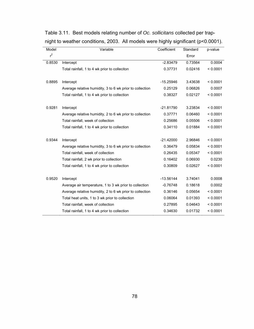
Table 3.11. Best models relating number of Oc. sollicitans collected per trap-
night to weather conditions, 2003. All models were highly significant (p<0.0001). Model
r2
Variable Coefficient Standard
Error
p-value
0.8530 Intercept -2.83479 0.73564 0.0004
Total rainfall, 1 to 4 wk prior to colleciton 0.37731 0.02416 < 0.0001
0.8895 Intercept -15.25946 3.43638 < 0.0001
Average relative humidity, 3 to 6 wk prior to collection 0.25129 0.06826 0.0007
Total rainfall, 1 to 4 wk prior to collection 0.38327 0.02127 < 0.0001
0.9281 Intercept -21.81790 3.23834 < 0.0001
Average relative humidity, 2 to 6 wk prior to collection 0.37771 0.06460 < 0.0001
Total rainfall, week of collection 0.25686 0.05506 < 0.0001
Total rainfall, 1 to 4 wk prior to collection 0.34110 0.01884 < 0.0001
0.9344 Intercept -21.42000 2.96846 < 0.0001
Average relative humidity, 3 to 6 wk prior to collection 0.36479 0.05834 < 0.0001
Total rainfall, week of collection 0.26435 0.05347 < 0.0001
Total rainfall, 2 wk prior to collection 0.16402 0.06930 0.0230
Total rainfall, 1 to 4 wk prior to collection 0.30809 0.02627 < 0.0001
0.9520 Intercept -13.56144 3.74041 0.0008
Average air temperature, 1 to 3 wk prior to collection -0.76748 0.18618 0.0002
Average relative humidity, 2 to 6 wk prior to collection 0.36146 0.05654 < 0.0001
Total heat units, 1 to 3 wk prior to collection 0.06064 0.01393 < 0.0001
Total rainfall, week of collection 0.27895 0.04643 < 0.0001
Total rainfall, 1 to 4 wk prior to collection 0.34630 0.01732 < 0.0001
78

In 2004, the smoothed data for rainfall in the current week explained both
the total number of mosquitoes collected per trap-night as well as the number of
Ae. vexans collected per trap-night (r2=0.3549 and 0.3564, respectively),
whereas numbers of Cx. tarsalis and Oc. sollicitans were dependent on the total
number of heat units four to eight weeks prior to collection (r2=0.8870 and
0.8530, respectively). Two-variable models for Ae. vexans and the total number
of mosquitoes collected included both the smoothing spline transformation for
rainfall in the current week as well as rainfall two to five weeks prior to collection
(r2=0.4886 and 0.4613, respectively). The best two-variable model for Cx.
tarsalis included total heat units four to eight weeks prior to collection and total
rainfall in the four weeks prior to collection (r2=0.5512), and for Oc. sollicitans the
model included total heat units three to five weeks prior to collection and rainfall
two to six weeks prior to collection (r2=0.7085). See Tables 3.12 through 3.15 for
complete model parameter estimates for the best models containing one to five
parameters for 2004.
79

Table 3.12. Best models relating total number of mosquitoes collected per trap-
night to weather conditions, 2004. All models were highly significant (p<0.0001). Model
r2
Variable Coefficient Standard
Error
p-value
0.3549 Intercept -88.15647 43.81136 0.0511
Smoothing spline parameter, rainfall, week of
collection
92.09318 19.88081 < 0.0001
0.4613 Intercept -162.01159 48.69764 0.0020
Total rainfall, 2 to 5 wk prior to collection 1.33914 0.48873 0.0093
Smoothing spline parameter, rainfall, week of
collection
89.04578 18.43804 < 0.0001
0.6067 Intercept -542.32777 103.26965 < 0.0001
Average air temperature, week of collection 12.94136 3.23546 0.0003
Total rainfall, 2 to 6 wk prior to collection 2.66498 0.56411 < 0.0001
Smoothing spline parameter, rainfall, week of
collection
102.24710 16.17090 < 0.0001
0.6532 Intercept -109.90798 219.82548 0.6201
Average air temperature, week of collection 11.60856 3.13879 0.0007
Average relative humidity, 2 to 5 wk prior to collection -8.74514 3.97645 0.0344
Total rainfall, 2 to 6 wk prior to collection 3.86175 0.76450 < 0.0001
Smoothing spline parameter, rainfall, week of
collection
111.32455 15.93633 < 0.0001
0.6953 Intercept -39.06484 211.44590 0.8545
Average air temperature, week of collection 12.43668 3.00756 0.0002
Average relative humidity, 2 to 5 wk prior to collection -11.09873 3.92883 0.0078
Total rainfall, 2 to 6 wk prior to collection 3.91623 0.72719 < 0.0001
Smoothing spline parameter, cumulative heat units
up to week of collection
0.08070 0.03670 0.0346
Smoothing spline parameter, rainfall, week of
collection
99.27709 16.11020 < 0.0001
80

Table 3.13. Best models relating number of Ae. vexans collected per trap-night
to weather conditions, 2004. All models were highly significant (p<0.0001). Model
r2
Variable Coefficient Standard
Error
p-value
0.3564 Intercept -96.62526 39.19890 0.0182
Smoothing spline parameter, rainfall, week of
collection
82.66306 17.78776 < 0.0001
0.4886 Intercept -170.35570 42.50328 0.0003
Total rainfall, 2 to 5 wk prior to collection 1.33688 0.42656 0.0033
Smoothing spline parameter, rainfall, week of
collection
79.62080 16.09271 < 0.0001
0.6016 Intercept 322.80629 156.90281 0.0468
Average relative humidity, 2 to 4 wk prior to collection -10.75871 3.32096 0.0025
Total rainfall, 2 to 5 wk prior to collection 3.24875 0.70275 < 0.0001
Smoothing spline parameter, rainfall, week of
collection
93.19741 14.99211 < 0.0001
0.6498 Intercept 224.70550 155.52362 0.1572
Average air temperature, 5 wk prior to collection 5.62957 2.53019 0.0324
Average relative humidity, 2 to 4 wk prior to collection -10.82734 3.15686 0.0015
Total rainfall, 2 to 5 wk prior to collection 3.47503 0.67569 < 0.0001
Smoothing spline parameter, rainfall, week of
collection
84.29403 14.80180 < 0.0001
0.8515 Intercept 682.91881 205.92069 0.0021
Average relative humidity, 1 to 5 wk prior to collection -25.09962 3.73160 < 0.0001
Total rainfall, 2 to 5 wk prior to collection 2.89818 0.38590 < 0.0001
Smoothing spline parameter, average air
temperature, week of collection
52.94027 4.82876 < 0.0001
Smoothing spline parameter, heat units, week of
collection
-102.28956 9.22328 < 0.0001
Smoothing spline parameter, cumulative heat units
up to week of collection
0.26097 0.02686 < 0.0001
81

Table 3.14. Best models relating number of Cx. tarsalis collected per trap-night
to weather conditions, 2004. All models were highly significant (p<0.0001). Model
r2
Variable Coefficient Standard
Error
p-value
0.4994 Intercept -2.35544 2.35667 0.3237
Total heat units, 4 to 8 wk prior to collection 0.06674 0.01070 < 0.0001
0.5512 Intercept 1.78237 3.00251 0.5563
Total heat units, 4 to 8 wk prior to collection 0.06551 0.01028 < 0.0001
Total rainfall, 1 to 4 wk prior to collection -0.06799 0.03247 0.0430
0.6397 Intercept -28.26596 10.33489 0.0095
Average relative humidity, 2 to 3 wk prior to collection 0.64486 0.21394 0.0046
Total heat units, 4 to 8 wk prior to collection 0.06297 0.00937 < 0.0001
Total rainfall, 1 to 4 wk prior to collection -0.19393 0.05114 0.0005
0.7605 Intercept -133.81884 16.86101 < 0.0001
Average air temperature, 1 to 5 wk prior to collection 1.92841 0.23906 < 0.0001
Average relative humidity, 2 to 6 wk prior to collection 2.17586 0.28978 < 0.0001
Total rainfall, 1 to 5 wk prior to collection -0.15149 0.03123 < 0.0001
Total rainfall, 3 to 7 wk prior to collection -0.13073 0.04090 0.0029
0.8606 Intercept -166.82932 14.43178 < 0.0001
Average air temperature, 1 to 5 wk prior to collection 3.45782 0.44949 < 0.0001
Average relative humidity, 2 to 6 wk prior to collection 2.60651 0.23539 < 0.0001
Total heat units, 1 to 2 wk prior to collection -0.13043 0.04993 0.0132
Total rainfall, 2 to 6 wk prior to collection -0.26819 0.03615 < 0.0001
Smoothing spline parameter, rainfall, week of
collection
-6.41886 1.09282 < 0.0001
82

Table 3.15. Best models relating number of Oc. sollicitans collected per trap-
night to weather conditions, 2004. All models were highly significant (p<0.0001). Model
r2
Variable Coefficient Standard
Error
p-value
0.6597 Intercept -1.75923 1.23249 0.1614
Total heat units, 4 to 7 wk prior to collection 0.06051 0.00696 < 0.0001
0.7085 Intercept -9.07197 2.42060 0.0006
Total heat units, 3 to 5 wk prior to collection 0.09722 0.01032 < 0.0001
Total rainfall, 2 to 6 wk prior to collection 0.07440 0.02042 0.0008
0.7182 Intercept -9.23812 2.41624 0.0005
Total heat units, 3 to 5 wk prior to collection 0.09580 0.01036 < 0.0001
Total rainfall, 1 to 5 wk prior to collection 0.02927 0.02588 0.2654
Total rainfall, 2 to 6 wk prior to collection 0.05000 0.02966 0.1002
0.7529 Intercept -28.63436 8.02246 0.0010
Average air temperature, week of collection 0.47088 0.20768 0.0295
Average relative humidity, week of collection 0.19007 0.07910 0.0216
Total heat units, 3 to 5 wk prior to collection 0.07423 0.01400 < 0.0001
Total rainfall, 2 to 6 wk prior to collection 0.10482 0.02348 < 0.0001
0.7949 Intercept -46.73821 8.11453 < 0.0001
Average air temperature, 2 to 5 wk prior to collection 1.41752 0.12286 < 0.0001
Average relative humidity, week of collection 0.25230 0.06737 0.0006
Average relative humidity, 1 to 4 wk prior to collection 0.24835 0.13467 0.0736
Total rainfall, 2 to 5 wk prior to collection 0.06665 0.02442 0.0099
Smoothing spline parameter, rainfall, week of
collection
-3.27970 0.78296 0.0002
83

Regression analysis indicated mosquito abundance was dependent upon
multiple weather variables in the weeks prior to mosquito collection. Most of the
best models containing one or two variables consisted of terms for rainfall and
heat units, and a few were also dependent upon relative humidity. Many of the
best models were based upon the weather conditions four to eight weeks prior to
collection. The dependence of mosquito abundance on weather conditions and
the lag in the response to weather conditions is not surprising when considering
the biology of the mosquito. Mosquito development from egg to adult typically
takes several days to a few weeks for completion. Therefore, rainfall and heat
several weeks prior to collection may produce suitable habitats for oviposition of
new eggs or hatching of quiescent eggs and time for them to complete
development.
Other studies have demonstrated similar relationships between weather
conditions and mosquito abundance. In Australia, unusually high rainfall led to a
population explosion of Oc. vigilax Skuse [65], similar to the population explosion
of Ae. vexans experienced in Lubbock during 2004. In San Antonio, TX,
oviposition in Cx. quinquesfasciatus was not dependent on rainfall but rather on
daily temperature, and oviposition was highest when maximum daily
temperatures exceeded 27°C and minimum daily temperature ranged from 18°C
to 24°C [66].
Associations between daily temperature and rainfall were also apparent
during a study conducted in southern California [67]. Flooding caused by
dredging the Colorado River and agricultural irrigation led to increases in Ae.
vexans populations. Irrigation of crops led to patchy abundance of Ps.
columbiae, and irrigation of windbreaks using sewer water increased populations
of Cx. quinquefasciatus. Additionally, hot summer and cool winter temperatures
decreased populations of Cx. tarsalis [67]. Populations of Cx. nigripalpus
Theobald were correlated with rainfall, and above-normal rainfall and
temperatures during 1991 in northeast Florida induced early-season populations
84

of Cx. nigripalpus [55]. Frequency of rainfall rather than total amount of rainfall
was useful in predicting populations of Ae. vexans, Ps. columbiae, and Ps.
howardii Coquillett in citrus-groves in Florida. The frequency of rainfall less than
12.7 mm determined populations of these species, with the critical value being
four consecutive weeks [68]. Larval populations of Ae. aegypti were predicted
based upon amount of rain and number of rainy days seven to eleven days prior
to collection [69].
Conclusions and Future Studies
An updated species distribution list for the mosquitoes of Lubbock, TX,
has been derived from the data collected over this three-year study period. In
2003, during a drought year, the dominant mosquito species collected was Cx.
tarsalis. The following year was extremely wet and the dominant species
collected during 2004 was Ae. vexans. Relationships between mosquito
collections and weather patterns were apparent in both the graphical displays of
the data as well as in the regression analysis. Weather conditions, specifically
rainfall and heat units in the four to eight weeks prior to mosquito collection, were
the best models included variables for the total number of mosquitoes collected
as well as the number of mosquitoes of dominant species collected. Landscape
features of mosquito trapping locations, such as vegetation and potential
breeding sites, also influenced mosquito communities. Future studies on
mosquito community dynamics will involve the enhancement of models for
predicting mosquito abundance as related to weather conditions and trapping site
characterization, as well as continued surveillance of mosquito communities for
the appearance of new species or the disappearance of current species of the
Lubbock area (Chapter VI).
85

CHAPTER IV
OVERALL INFLUENCES AND DRIVERS OF WEST NILE VIRUS
OCCURRENCE AND TRANSMISSION
Introduction and Research Goals
Mosquitoes and Disease Transmission
Although mosquitoes are known to most people as pests, they are also of
very significant public health and veterinary importance because they feed on
human and animal blood and may thereby transmit diseases [37]. The blood-
feeding process (as discussed in Chapter III) introduces mosquito saliva
containing foreign proteins into the host’s bloodstream, resulting in a histamine
reaction that may be antigenic and lead to hypersensitivity. Blood feeding also
creates a wound at the bite site that may allow for secondary infection by
bacteria or other microorganisms [37]. In addition, microorganisms that cause
disease may be directly introduced or transmitted during blood feeding.
Diseases transmitted by mosquitoes typically fall into three categories: viruses,
malaria protozoans, and filarial nematodes [37]. Additionally, Francisella
tularensis (causative agent of tularemia) is transmitted by Aedes cinereus
Meigen in Sweden [70]. Mechanical transmission of F. tularensis and Bacillus
anthracis (causative agent of anthrax) is also known to occur [37].
Viruses. Of the over 520 viruses transmitted by arthropods (arboviruses),
approximately half of these are transmitted by mosquitoes [37]. About 100 of
these are zoonoses and infect humans as well as animals, with the most
significant of these viruses belonging to four genera in three families [37]. The
family Togaviridae, genus Alphavirus, includes eastern equine encephalitis
(EEE), western equine encephalitis (WEE), Venezuelan equine encephalitis
(VEE), and Ross River virus among others. The family Flaviviridae, genus
Flavivirus, includes dengue, yellow fever, Japanese encephalitis, and St. Louis
encephalitis (SLE) among others. The family Bunyaviridae, genus Bunyavirus,
86

includes California encephalitis, Jamestown Canyon virus, and La Crosse
encephalitis among others. Also included in the family Bunyaviridae is the genus
Phlebovirus, which includes Rift Valley Fever. These viruses may be transmitted
by a wide range of mosquito vector species, including those belonging to the
genera Aedes, Culex, Culiseta, Ochlerotatus, Psorophora, and others [37].
Most mosquito-borne viruses are similar in the disease symptoms they
cause, generally flu-like symptoms, including fever as well as joint and muscle
pain [37]. Hemorrhagic fever and encephalomyelitis may also occur. Although
morbidity may be high for cases involving fever, the case mortality rate is
generally low. Morbidity and mortality for encephalitis and hemorrhagic fevers
range from low to high depending upon the virus as well as other factors
including the victim’s age. Although chronic illness does not often occur in
humans with these mosquito-borne viruses, the consequences of these
infections may be long-lasting. Additionally, since these viruses have RNA
(ribonucleic acid) genomes and are capable of multiplying in both vertebrate and
invertebrate cells, they have the capacity to rapidly evolve into antigenically
variable strains with widespread virulence, which may result in the emergence of
highly virulent, epidemic strains [37].
The mechanisms of transmission of mosquito-borne viruses are fairly well
known. Arboviruses cause cytopathic effects and cell destruction in vertebrate
cells; however, chronic cellular infection without cytopathology occurs in
invertebrate cells [37]. If a vertebrate host has a sufficient amount of circulating
virus in its blood to provide an infectious dose to the mosquito, the mosquito
becomes infected during blood feeding. The blood enters the midgut of the
mosquito and virions bind to and pass through the microvilliar membrane and
into midgut epithelial cells. The viruses then replicate and virions bud off from
the cells. Virions pass through the basal lamina, enter the hemolymph, and are
then disseminated throughout the body of the mosquito to infect and replicate in
the mosquito’s tissues, including salivary glands, fat bodies, ovaries, and nerves.
87

Transmission of infectious virions to another host occurs when a mosquito (with a
salivary gland infection) salivates as it probes the tissue of a host [37].
Transovarial transmission, in which the female mosquito infects her progeny,
allows females of the next generation to transmit the virus during their first blood
meal. Venereal transmission from male to female mosquitoes has also been
documented for some species of mosquitoes and some viruses [37].
Malaria Protozoans. Malaria is transmitted by Anopheline mosquitoes and
although indigenous malaria has been eradicated from the United States, it is
one of the most widespread (Figure 4.1) and prevalent infectious human
diseases [37]. Travelers to endemic areas may become infected during their
travels. Approximately 1.6 billion people are at direct risk of acquiring malaria
from a mosquito bite. There are an estimated 300 to 500 million world-wide
cases reported yearly, with the most devastating effects occurring in sub-
Saharan Africa where 100 million cases and more than one million deaths occur
each year due to the disease [37]. The disease is caused by sporozoan protists
in the family Plasmodiidae, genus Plasmodium (order Haemosporidida, class
Haemosporidea, phylum Sporozoa). Four species are known to cause malaria in
humans including Plasmodium falciparum, P. vivax, P. malariae, and P. ovale.
There are many additional species that infect reptiles, birds, rodents, and
nonhuman primates as well. [37].
88

Figure 4.1. Estimate of world malaria burden, with intensity of blue indicating
increasing burden of malaria [71].
Plasmodium species are obligate intracellular parasites and their complex
life cycle involves both sexual and asexual reproduction [37]. The sexual phase
or gametogony begins in the blood of the human host and ends in the lumen of
the midgut of the mosquito. The first phase of asexual reproduction (sporogony)
occurs on the outer wall of the midgut and is referred to as the exogenous phase
of malaria parasite development. The second phase of asexual reproduction
(merogony or schizogony) occurs in the liver and blood of the human host and is
therefore referred to as the endogenous phase of malaria parasite development.
The complete life cycle is depicted in Figure 4.2 [37].
89

Figure 4.2. Life cycle of Plasmodium spp. in human and Anopheles hosts [41].
Filarial Nematodes. Filariasis is the disease characterized by the infection
of vertebrate tissue by nematodes or roundworms (phylum Nematoda, order
Spirurida, superfamily Filarioidea, family Onchocercidae). Wuchereria bancrofti,
Brugia malayi, and B. timori are the three causative agents of lymphatic filariasis
and are associated with acute and chronic disease in humans [37]. Disease
occurrence is not as extreme as that of malaria, but approximately 900 million
people are at risk of contracting the disease worldwide, with 43 million having
chronic infections. Mosquitoes in the genera Culex, Mansonia, Aedes,
Ochlerotatus, and Anopheles are important in the transmission of filariasis [37].
The transmission mechanism of filariasis is called contaminative rather
than inoculative as in other transmission cycles [37]. Rather than having
microorganisms injected into the host’s system during blood feeding, third-stage
infective larvae exit the labium of the proboscis, crawl onto the skin surface, and
90

enter the host’s system through the wound at the site of the mosquito bite. The
nematodes then molt twice, travel to the lymphatic vessels and lymph nodes, and
complete development to the adult stage. There, female worms release active,
immature worms into the peripheral circulatory system. These can then be
ingested by mosquitoes during blood feeding, with immature worms completing
their development in the mosquito to become infective, third-stage larvae.
Human disease rarely occurs with the bite of a single, infective mosquito.
Typically, repeated (hundreds to thousands) of such bites under conditions
favorable to parasite maturation and mating are required [37].
Although human lymphatic filariasis is typically not a problem in the United
States, dog heartworm caused by the mosquito-borne filarial nematode Dirofilaria
immitis (family Onchocercidae) does occur throughout the country, with at least
20 species of mosquitoes found to be infected [37]. Adult nematodes (12 to 31
cm long) form aggregations of up to 50 or more individuals in the right ventricle of
the canine heart and pulmonary arteries. These aggregations cause changes in
the endothelium and integrity of the walls of the pulmonary arteries. Decreased
cardiac output to the lungs, weakness, lethargy, and congestive heart failure
result from pulmonary hypertension and right ventricular hypertrophy [37].
West Nile Virus Classification and Structure
West Nile virus (WNV) belongs to the genus Flavivirus in the family
Flaviviridae and is a member of the Japanese Encephalitis Antigenic Complex
[72]. Additional viruses in this complex include Kunjin virus, Murray Valley
encephalitis, and SLE. As with other Flaviviruses, WNV is a positive-sense,
single-stranded RNA virus [72]. The virus is approximately 500 Å in diameter
and has icosahedral symmetry with no surface projections or spikes [73]. The
virus consists of multiple layers with the outermost layer containing
transmembrane proteins E and M. The next layer is a 35 to 40-Å thick lipid
bilayer which surrounds the nucleocapsid core containing the RNA genome.
91
Protein E is the major surface protein and is responsible for receptor binding,
host membrane fusion, and is also capable of eliciting a neutralizing antibody
response [73].
West Nile Virus History and Distribution
International. West Nile virus was first isolated in 1937 in the West Nile
District of Uganda from a febrile adult woman [74]. Its ecology was later
characterized in the 1950s in Egypt. In 1957, the virus was found to be
responsible for an outbreak of severe human meningitis in elderly patients in
Israel, followed by its first appearance as an equine disease in the early 1960s in
Egypt and France [74]. Since then, WNV has been reported in Africa, Europe,
the Middle East, west and central Asia, Oceania, and North America [74].
Recent outbreaks of WNV in humans have occurred in Algeria (1994),
Romania (1996 and 1997), Czech Republic (1997), the Democratic Republic of
Congo (1998), Russia (1999), the United States (1999 through 2004), and Israel
(2000). Recent outbreaks have also occurred in horses in Morocco (1996), Italy
(1998), the United States (1999 through 2001), and France (2000), with
additional outbreaks of disease in birds in Israel (1997 through 2001) and the
United States (1999 through 2002) [74]. Figure 4.3 displays the approximate
geographic range of WNV as of 2002.
92

Figure 4.3. The approximate geographic range of WNV (yellow) as of 2002.
Modified from Campbell and others [75]. The worldwide distribution of WNV by
the end of 2004 extended throughout the entire continental United States.
United States. When WNV first appeared in the United States in late
August 1999, it was originally thought to be an act of bioterrorism. The Central
Intelligence Agency soon investigated and determined that the outbreak of WNV
was highly unlikely to be caused by terrorist [76]. Regardless, the identification
of a cluster of four cases of unusual encephalitis associated with muscle
paralysis in the New York City area, an area that typically has only nine,
dispersed cases of encephalitis per year, prompted the New York City
Department of Health to initiate an outbreak investigation [77]. The identification
of this cluster in a small area of the city was largely due to recent actions by the
Health Department promoting the importance of physicians reporting unusual
disease clusters or manifestations. Although routine surveillance for viral
meningitis or encephalitis did not indicate a departure from historical trends in the
area, a physician reported an unusual disease manifestation, which resulted in
the initial recognition of the human outbreak of WNV [77].
93

Within two days of the launch of the outbreak investigation, eight suspect
cases were identified in nearby hospitals, all of which presented nearly identical
symptoms including febrile illness with mild gastrointestinal symptoms, followed
by the onset of altered mental status [77]. Most of these patients also had
severe, diffuse muscle weakness with half developing paralysis requiring
ventilatory support. Additionally, all of these patients were from a 40 km2 area of
northern Queens and the patients did not know each other or have any common
exposures due to travel, social events, restaurants, or commercial food items.
However, all of these patients reported spending time outdoors, especially in the
evening hours. Through environmental investigations, Culex spp. breeding sites
and larvae were found in most of the patients’ yards or neighborhoods [77].
As the investigation was extended to include all of New York City, 30
suspect cases throughout the city were identified by the beginning of September
1999 [77]. Initial laboratory testing incriminated SLE virus as being responsible
for the disease outbreak. It was not until three weeks after the initial outbreak of
human disease that WNV was determined to be responsible for the outbreak.
Until WNV was determined to be the causative agent, substantial bird die-offs,
concurrent with the human disease outbreak, were thought to be coincidental
since SLE typically does not cause avian mortality [77]. Observations of
encephalitis and viral inflammation of other organs in birds prompted further
investigation by veterinarians and wildlife specialists. West Nile virus was
identified in avian tissue specimens and also found to be the etiologic agent
responsible for the outbreak in birds, horses, and humans. The virus was also
isolated from Culex pipiens Linnaeus mosquitoes collected from the area where
the epidemic occurred [77].
In 1999, only New York, Connecticut, New Jersey, and Maryland were
affected by the outbreak of WNV. In 2000, WNV spread to nearby states
including Vermont, New Hampshire, Massachusetts, Rhode Island,
Pennsylvania, Delaware, Vermont, and North Carolina, as well as the District of
94

Columbia. By 2001, the outbreak had spread to most states east of the
Mississippi River. In 2002, the virus spread across the United States, and by the
end of 2003, Oregon, Alaska, and Hawaii were the only states that had not seen
their first case of WNV. Oregon saw its first WNV cases in 2004, but Alaska and
Hawaii still have not observed WNV. See Figure 4.4 [78-81].
Figure 4.4. The spread of WNV across the United States, 1999 through 2004.
Modified from the Centers for Disease Control and Prevention (CDC) maps and
figures [78-81].
Texas. Texas saw its first cases of WNV in 2002. That year there were
approximately 200 human cases in 37 counties and about 1700 horse cases in
204 counties, in addition to many positive results from bird and mosquito
specimens. West Nile virus continued to appear in Texas in 2003 and 2004 [82].
Throughout 2002 to 2004, WNV was detected in nearly every county in Texas
(Figure 4.5) in birds, humans, mosquitoes, horses, other animals, or in
combinations of these [83-85].
95

Figure 4.5. Texas counties with WNV-positive (blue) bird, mosquito, horse, other
animal, or human cases, 2002 through 2004. Modified from the Texas
Department of State Health Services Statistics [83-85].
Of the 22 counties with no reported WNV, four of these have a population
of less than 25,000 people, three of them have a population less than 10,000
people, 10 have a population less than 5000 people, and five of them have a
population of less than 1000 people. Population density in these counties ranged
from 23 to 0.1 people per 1.6 km2 [86]. Lack of WNV in a county could be
misleading depending on if this is due to restrictions on resources that prevent
WNV surveillance operations or if screening for WNV has been ongoing and
there truly is no WNV in the area. Additionally, many counties with populations
less than 20,000 people that reported cases in 2002 had no WNV cases reported
during 2003 and 2004, which could also be an artifact of limited surveillance
operations [83-85].
96

In 2002, half the human cases reported in Texas were from Harris County.
Although there were 105 human cases in the Houston area that year, comparing
this number to the population of Harris County revealed that there were only
three human cases per 100,000 people. In 2003, Texas had 439 human cases
of WNV. That year, Harris County only reported 43 human cases, whereas
Lubbock County and Randall County had 26 and 20 human cases, respectively.
When comparing these numbers to population size, Lubbock County had
approximately 11 cases per 100,000 people and Randall County had almost 20
cases per 100,000 people whereas Harris County only had about one case per
100,000 people. The number of human cases in 2004 was much lower with only
118 cases reported [83-86].
Lubbock, Texas. West Nile virus was first detected in Lubbock, TX
(33.65°N, 101.81°W, 975 m elevation), as a result of this research project. The
first WNV-positive mosquitoes were collected in late summer 2002 [87].
Although there were no human cases of WNV in 2002, they began to appear in
2003 with a total of 26 human cases in Lubbock County that year [88].
West Nile Virus in Mosquitoes
As stated previously, WNV is transmitted to humans and other animals by
blood-feeding mosquitoes, primarily those belonging to the genus Culex [89].
During 1999, only four species of mosquitoes were found to be infected with
WNV. As the virus became more established and moved across the United
States, however, additional species of mosquitoes were found to be infected [90].
Table 4.1 lists all field-collected species of mosquitoes that have tested positive
for WNV from 1999 through 2004 and those species that are located in the
Lubbock area.
97
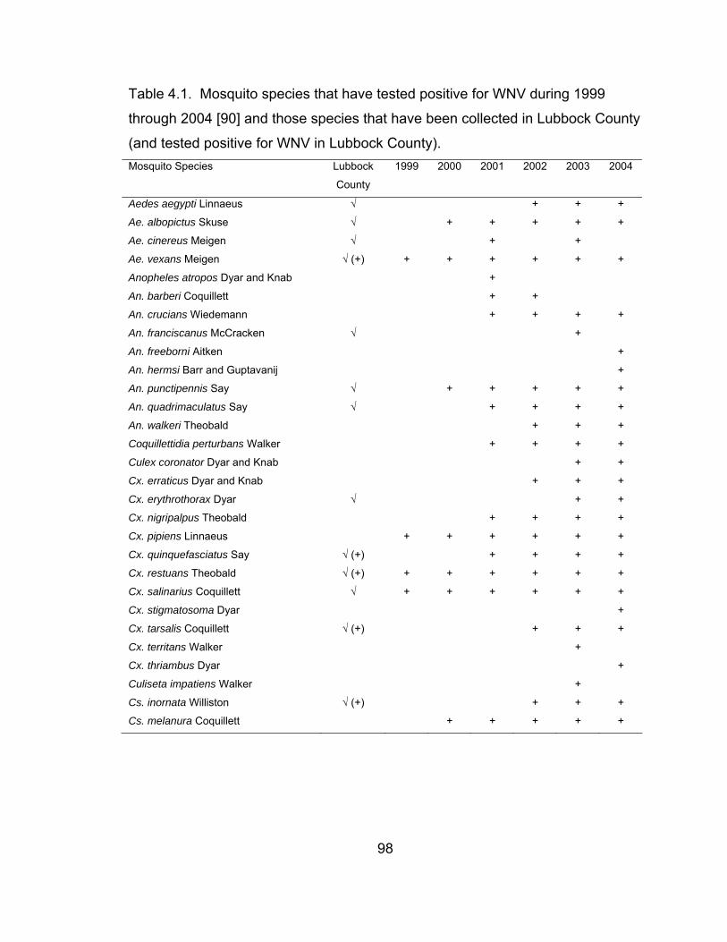
Table 4.1. Mosquito species that have tested positive for WNV during 1999
through 2004 [90] and those species that have been collected in Lubbock County
(and tested positive for WNV in Lubbock County). Mosquito Species Lubbock
County
1999 2000 2001 2002 2003 2004
Aedes aegypti Linnaeus √ + + +
Ae. albopictus Skuse √ + + + + +
Ae. cinereus Meigen √ + +
Ae. vexans Meigen √ (+) + + + + + +
Anopheles atropos Dyar and Knab +
An. barberi Coquillett + +
An. crucians Wiedemann + + + +
An. franciscanus McCracken √ +
An. freeborni Aitken +
An. hermsi Barr and Guptavanij +
An. punctipennis Say √ + + + + +
An. quadrimaculatus Say √ + + + +
An. walkeri Theobald + + +
Coquillettidia perturbans Walker + + + +
Culex coronator Dyar and Knab + +
Cx. erraticus Dyar and Knab + + +
Cx. erythrothorax Dyar √ + +
Cx. nigripalpus Theobald + + + +
Cx. pipiens Linnaeus + + + + + +
Cx. quinquefasciatus Say √ (+) + + + +
Cx. restuans Theobald √ (+) + + + + + +
Cx. salinarius Coquillett √ + + + + + +
Cx. stigmatosoma Dyar +
Cx. tarsalis Coquillett √ (+) + + +
Cx. territans Walker +
Cx. thriambus Dyar +
Culiseta impatiens Walker +
Cs. inornata Williston √ (+) + + +
Cs. melanura Coquillett + + + + +
98

Table 4.1. Continued. Mosquito Species Lubbock
County
1999 2000 2001 2002 2003 2004
Cs. morsitans Theobald + +
Deinocerites cancer Theobald +
Mansonia tittilans Walker +
Ochlerotatus atlanticus/tormentor Dyar
and Knab/Dyar and Knab
√ + +
Oc. atropalpus Coquillett +
Oc. canadensis Theobald + + + + +
Oc. cantator Coquillett + + +
Oc. condolescens Dyar and Knab +
Oc. dorsalis Miegen √ +
Oc. dupreei Coquillett +
Oc. fitchii Felt and Young +
Oc. fulvus-pallens Wiedemann +
Oc. grossbecki Dyar and Knab +
Oc. infirmatus Dyar and Knab +
Oc. japonicus Theobald + + + + +
Oc. melanimon Dyar +
Oc. nigromaculis Ludlow √ + +
Oc. provocans Walker +
Oc. sollicitans Walker √ (+) + + +
Oc. squamiger Coquillett +
Oc. sticticus Meigen + +
Oc. stimulans Walker √ +
Oc. taeniorhynchus Wiedemann √ + + +
Oc. triseriatus Say √ + + + + +
Oc. trivittatus Coquillett + + + + +
Orthopodomyia signifera Coquillett + +
Psorophora ciliata Fabricius √ (+) +
Ps. columbiae Dyar and Knab √ + + + +
Ps. ferox Humboldt + + +
Ps. howardii Coquillett + +
Uranotaenia sapphirina Osten Sacken √ + + + +
99

It should be cautioned that despite the sizable list in Table 4.1, the
detection of WNV in a given mosquito species does not mean that the species is
a vector of WNV. Vector competency tests have been conducted on various
species of mosquitoes in order to determine the ability of a given mosquito
species to transmit WNV [91]. Adequate control programs are based upon the
vector status of potential vectors. In order to incriminate a mosquito species as a
vector, it must be shown to transmit WNV through a bite. Its importance as a
vector is then determined based upon population density, host preference,
feeding behavior, longevity, and seasonal activity [91]. Repeated detection of
virus from field-collected individuals is not enough to implicate a species as a
confirmed vector because those individuals may not be capable of transmitting
the virus by blood feeding. The ability of the species to become infected and
transmit the virus in the laboratory and an association in nature between the
species and a vertebrate hosts are additional criteria that must be met to deem a
specific species a vector of WNV [92].
Feeding behavior is an important aspect to consider when determining the
efficiency of a mosquito vector for transmission of WNV [92]. For example, some
mosquitoes feed preferentially on birds and thus might be important in amplifying
and maintaining WNV, but they would be relatively unimportant in transmitting
the virus to humans or horses. Some mosquitoes are also known to change their
feeding preference based upon season or host availability. These species may
play an important role in amplifying and maintaining the virus early in the season,
but as bird communities change (by migration, for example) and mammals
become more prevalent later in the season, their importance as a vector may
shift to becoming a serious risk to humans and horses. Other mosquitoes are
opportunistic feeders and may be important bridge vectors in that they may feed
on a viremic bird and later pass the virus on to a susceptible mammalian host
[92].
100

A recent study by Terell and others compiled data on studies that were
conducted to determine the vector competence of North American mosquitoes as
well as several other species in which WNV had been isolated in nature but for
which no data existed on their ability to transmit the virus [92]. For nearly all the
mosquito species they studied, although the susceptibility to WNV varied among
species, if the mosquito developed a disseminated infection (virus recovered
from both leg and body suspensions), it was able to transmit the virus by bite.
From their study, Culex spp., especially Cx. pipiens, Cx. restuans, Cx. salinarius,
and Cx. tarsalis, were important vectors because laboratory studies showed
them to be extremely efficient vectors, there have been many field isolations of
WNV from these species, and they have a high potential to serve either as an
enzootic (maintenance) vector or epizootic (bridge) vector or both [92]. Other
species, such as Aedes spp., Culiseta spp., and Ochlerotatus spp., may be
efficient vectors in the lab, but there have been few field isolations of WNV in
these species and they have a lower potential to serve as enzootic or epizootic
vectors [92].
The risk of a mosquito species transmitting WNV to humans can also be
calculated. Risk, in this sense, is based upon the abundance of that species,
fraction of blood meals taken from mammals, WNV infection prevalence, and
vector competence [93]. Using this calculation, control efforts can be focused on
one or a few specific species, thereby reducing detrimental effects on non-target
species and improving the effectiveness of control measures. By actively
targeting species with the highest risk of transmitting WNV to humans, the
number of human WNV cases should decrease; this would potentially reduce
transmission of WNV in birds and decrease the severity of WNV epidemics in
birds and, consequently, in mammalian communities [93]. However, the risk
calculation is sensitive to spatial and geographic context and must be calculated
based upon potential vectors in a given area at a given time. Competent vectors
with a high risk of transmission to humans in one region may be different than
101
those in another region. Mosquito species with the highest risk of transmission of
disease to humans may also change throughout the transmission season
depending upon host switching and host and mosquito relative abundances
throughout the season. The risk calculation may also be used to predict the
number of human cases in a transmission season based upon the sum of risk
over all mosquito species and the human population density in a given area, but
this has not yet been validated [93].
West Nile Virus Screening Methods
Although several methods have been developed for screening mosquitoes
and animal tissues for WNV, reverse-transcriptase polymerase chain reaction
(RT-PCR) and the VecTest® Antigen Assay (Medical Analysis Systems, Inc,
Camarillo, CA) are the two methods that are used most often and were the
methods utilized in this study, therefore only these methods are discussed.
Reverse-Transcription Polymerase Chain Reaction. Although the PCR
(polymerase chain reaction) procedure is used for amplification of segments of
DNA (deoxyribonucleic acid), in RT-PCR, reverse transcriptase is used to
synthesize cDNA from the RNA template. Enzymatic amplifications of the cDNA
are then performed using PCR. Prior to the introduction of the use of RT-PCR,
WNV detection and identification was conducted by mouse and cell culture
inoculation with serologic identification of isolates, a laborious process that took
days to weeks to complete [94]. A more rapid procedure was needed, so Porter
and others evaluated PCR for its sensitivity and specificity to identify WNV [94].
Polymerase chain reaction was shown to be effective, and no cross-reactivity
occurred between WNV primers and Japanese encephalitis, SLE, or yellow fever
viruses. Cross-reactivity did occur between WNV and Kunjin virus, but this was
expected due to their homology in nucleotide and amino acid sequences.
Despite this, the RT-PCR assay was deemed useful in epidemiological
investigations of WNV infections [94].
102
Although the method developed by Porter and others [94] was highly
sensitive and specific, primers were designed using the published sequence for
the Uganda 1939 WNV strain. Identification of the viral strain responsible for the
1999 outbreak of WNV resulted in the identification of a new WNV isolate, NY99,
that demonstrated only 79% homology with the Uganda 1939 strain [95]. Thus
Lanciotti and others [95] evaluated the TaqMan exonuclease assay for use in
detecting WNV in human clinical specimens, field-collected mosquitoes, and
avian samples using RT-PCR. The TaqMan assay displayed increased
sensitivity compared to traditional RT-PCR assays. Reverse-transcriptase
polymerase chain reaction assays may be subject to inhibition due to the large
quantity of proteins and lipids present in mosquito pools which may inhibit either
the RT or the Taq polymerase enzyme. The TaqMan assay may also be more
sensitive because it amplifies smaller DNA fragments and does not require the
synthesis of full-length DNA products. The TaqMan assay was also highly
specific in that no false-positive results were observed [95].
Reverse-transcriptase polymerase chain reaction has been optimized for
use in detecting WNV in avian tissues as well. Although brain tissue is the most
sensitive target organ and generally used for screening birds, the use of heart,
lung, liver, kidney, and spleen tissues are also acceptable [96]. Oral and cloacal
swab samples have also shown to be accurate and cost-effective for screening
dead birds for WNV [97]. Additionally, feather pulp was also found to be a good
source of WNV as well as being a non-lethal technique for screening live birds
[98].
VecTest® Antigen Assay. The outbreak and rapid spread of WNV in North
America demonstrated the need for a rapid method to screen field-collected
mosquitoes for arboviral antigens [99]. The VecTest® Antigen Assay was
developed to meet this need. The VecTest® is a lateral flow wicking assay that
utilizes immunochromatographic technology to screen for type-specific
monoclonal antibodies against WNV and SLE antigens. This wicking assay is
103

available as a kit and is a simple and rapid test in that results are available in less
than 20 minutes. In addition, no specialized equipment or highly trained
personnel are required. The test is available as antigen assays for detecting
WNV or SLE or as an antigen panel assay for detecting both arboviruses in
combination [99].
With this test, monoclonal antibodies were selected and either immobilized
as capture antibodies in the test zone of the dipstick or conjugated with colloidal
gold in the reagent zone of the dipstick [99]. When the dipstick is inserted into
the mosquito homogenate, antigen present in the tissue binds to the specific
antibody-gold conjugate in the reagent zone. This antigen-antibody-gold
complex then migrates through the test zone of the dipstick, binds to the
immobilized antibody, and produces a reddish-purple line in the corresponding
area of the dipstick when WNV or SLE antigen is present. Unbound complexes
migrate out of the test zone and are captured in the control zone. This control
zone serves as an internal check that the test has been performed correctly and
that the homogenate suspension successfully migrated through the test zone of
the dipstick [99].
The VecTest® Assays have previously been evaluated for their specificity
and sensitivity [99]. For the antigen assays, there was no cross-reactivity with
the two viruses in that SLE antigen was not detected with the WNV Antigen
Assay and WNV antigen was not detected with the SLE Antigen Assay [99].
Each assay also produced a clear positive result for corresponding antigens with
WNV antigen diluted up to 1/1000 and SLE antigen diluted up to 1/10,000. The
panel assay displayed similar results in that WNV antigen diluted 1/1000 and
SLE antigen diluted 1/10,000 were both detected both separately and when
combined [99]. In evaluations of laboratory-infected mosquitoes, the tests were
able to detect a single virus-positive mosquito in a pool of 50 mosquitoes and
accurately identify the virus antigen in that pool. These evaluations also indicted
that there was no cross-reactivity. In addition, none of the virus-negative
104
mosquito pools gave a false positive result. Only a small number of field-
collected mosquitoes was analyzed, but similar results were obtained as in
laboratory-infected mosquitoes [99].
Although these evaluations showed the VecTest® was both sensitive and
specific with results comparable to that of antigen capture enzyme-linked
immunosorbent assay but less than that of Vero cell plaque assays or RT-PCR,
the test is still considered experimental, and results from field-collected
mosquitoes should be validated using another test [99]. Assays that detect
specific RNA sequences (such as RT-PCR) are used to validate VecTest®
results. The grinding medium used in the VecTest® reduces virus viability and so
cell culture assays should not be used. Field-collected mosquitoes that test
negative for viral antigen using the VecTest® should also be verified using RT-
PCR to determine the proportion of false-negatives [99].
The VecTest® Antigen Assay has also been used to screen birds for WNV
[100-104]. Previously, it was determined that cloacal and oral swabs could
replace brain tissue for screening birds for WNV [97]. With this and the need to
make dead-bird surveillance more cost-effective, the VecTest® was analyzed for
its ability to detect antigens in fecal, saliva, and tissue samples. Yaremych and
others [100] found the VecTest® produced three false-positives in comparison
with RT-PCR, but stated that the VecTest® may be a cost-effective and rapid field
technique for detection of WNV in dead birds. However, the use of the VecTest®
in dead birds is experimental and results need to be validated in the laboratory
using other testing methods [100]. Lindsay and others [102] made similar
conclusions after evaluating the VecTest® sensitivity and specificity for detecting
WNV in oropharyngeal and cloacal swabs from corvids in Canada, and Henson
and Hicock found 100% accuracy in testing cloacal swabs from corvids in
Mississippi [101]. A larger-scale study [103] conducted on many different bird
species in New York State found results comparable with Yaremych and Lindsay.
In addition, House Sparrows, House Finches, and Northern Cardinals could also
105
be used for surveillance of WNV in urban or suburban areas where corvid
populations have been diminished. In the Stone and others study [103], feather
pulp was also found to be a reliable antigen source, especially for testing live
birds. The majority of false-positive results identified in this study involved the
occurrence of narrow, faint lines that developed at the lower border of the test
region and intensified after 15 minutes had elapsed and true-positive tests had
developed to their full extent. The cause of these potentially misleading lines
was not determined, but in most cases they could be distinguished from true-
positive readings [103]. In using the VecTest® to test owls and diurnal raptors for
WNV, the assay was highly sensitive for detecting antigen in northern owl
species, but low sensitivity was observed in southern owl species and diurnal
raptors [104].
Research Goals and Hypotheses
The objective of this portion of the project was to model factors involved in
WNV maintenance and transmission. Appearance of WNV-positive mosquito
pools was related to weather conditions, including air temperature, precipitation,
relative humidity, weekly heat units, and cumulative heat units. Additionally,
relationships between mosquito collections and WNV occurrence were also
determined. Understanding environmental triggers of WNV emergence will aid in
developing and instituting focused surveillance and control operations. It is
hypothesized that WNV transmission in mosquitoes will be influenced by vector
populations and ultimately by weather conditions in the weeks prior to collection
of WNV-positive mosquitoes.
Materials and Methods
Mosquito Collection and Identification
Mosquito collection was conducted as previously described in Chapter III.
Encephalitis virus surveillance (EVS) light traps, CDC ultraviolet light traps, and
106
New Jersey light traps were used to collect mosquitoes throughout Lubbock
County throughout 2002 through 2004. Mosquitoes were identified to species,
pooled into groups of 50 mosquitoes or less, and stored at -80°C until
processing.
Weather Data
Data regarding weather conditions were collected as described in Chapter
II. Daily weather conditions were obtained from the United States Department of
Agriculture, Agricultural Research Service. The study years were then compared
to 30-year averages obtained from the National Oceanic and Atmospheric
Administration, National Climatic Data Center.
Screening for West Nile Virus
Since male mosquitoes do not take a blood meal and therefore are not
able to transmit disease, only female mosquitoes were screened for WNV. In
2002, all female mosquitoes collected using EVS light traps were screened for
WNV antigens using the VecTest® Antigen Assay, but samples were
inadvertently discarded and, therefore, results of the VecTest® were not validated
using RT-PCR. In 2003 all female mosquitoes collected were screened using the
VecTest® until WNV-positive mosquitoes began to appear throughout Lubbock
County. VecTest® screening was then reduced to one pool per species per site
per week. For sites where less than 50 mosquitoes of a species were collected
in a week, sites within that quadrant of the city were pooled. Also, since most
Cx. tarsalis mosquitoes were WNV-positive, this species was no longer tested
during 2003. VecTest® results were confirmed using RT-PCR, as well as
screening the remaining pools of female mosquitoes. For 2004, one pool per site
per week of Cx. tarsalis was tested using the VecTest® and these results were
verified with RT-PCR. All remaining Culex pools and all pools of mosquitoes not
previously tested in Lubbock County (Oc. zoosophus Dyar and Knab, Oc.
107

triseriatus, and Oc. thelcter Dyar) as well as two pools per week from two
randomly selected locations of Ae. vexans, Cs. inornata, Oc. dorsalis, and Oc.
sollicitans were also tested using RT-PCR.
Results of WNV were standardized by calculating the weekly minimum
infection rate (MIR) [93]. The number of WNV-positive pools was divided by the
total number of mosquitoes tested. This number was then multiplied by 1000 to
obtain the MIR.
Reverse-Transcription Polymerase Chain Reaction. Mosquitoes for RT-
PCR analysis were pooled by species, week, and trapping location into groups of
40 mosquitoes or less. TRI-Reagent® (Sigma-Aldrich, St. Louis, MO) was used
to extract RNA from the mosquitoes according to the manufacturer’s protocol
included in Appendix C and described here. TRI-Reagent® is a mono-phase
solution that combines phenol and guanidine thiocyanate to facilitate immediate
and effective inhibition of RNase activity. Mosquitoes were homogenized in STE
[10 mM NaCl (Sigma-Aldrich), 10 mM Tris HCl (Fisher Scientific, Houston, TX),
and 1 mM EDTA (Fisher Scientific)] containing 0.4 mg/ml Proteinase-K (Pierce,
Milwaukee, WI) and immediately placed on ice before proceeding with the
extraction. For samples containing 20 mosquitoes or less, 250 µL of STE and
500 µL of TRI-Reagent® was added to each sample, samples were ground, and
another 500 µL of TRI-Reagent® was added to each sample. For samples
containing more than 20 mosquitoes, 500 µL of STE was added to each sample,
samples were homogenized, and 100 µL of the homogenate was removed to a
new tube containing 1 mL of TRI-Reagent®. For confirmation of VecTest®
results, 100 µL of the VecTest® slurry was removed to a new tube containing 1
mL of TRI-Reagent®. Chloroform (200 µL, Sigma-Aldrich) was then added to
each homogenate and samples were incubated at room temperature for 15
minutes, followed by centrifugation in a microcentrifuge at 4°C at 12,000 xg for
15 minutes to allow for phase separation of RNA into the aqueous phase and
DNA into the interphase while proteins remained in the organic phase. Samples
108

were removed from the microcentrifuge to a sterile, laminar flow hood (The Baker
Company, Sanford, ME). The RNA fraction (350 µL) was then removed to a new
microcentrifuge tube and RNA was precipitated from the samples with 650 µL of
isopropanol (Sigma-Aldrich). Samples were allowed to precipitate in a -20°C
freezer for at least 10 minutes before continuation with another centrifugation at
4°C at 12,000 xg for eight minutes. The aqueous layer was removed from the
tube and RNA pellets were washed using 1 mL of 75% ethanol (Texas Tech
University Department of Chemistry and Biochemistry, Lubbock, TX). Samples
were again centrifuged for two minutes and the aqueous layer was removed.
Dried RNA samples were resuspended in 100 µL of RNAse-free water (Fisher
Scientific) and stored at -20°C.
Samples were analyzed for the presence of WNV using the Access
Quick™ RT-PCR protocol (Promega, Madison, WI), which is included in
Appendix C and described here. From the samples, RNA (5 µL) was added to
45 µL of the RT-PCR reaction mix for a total volume of 50 µL. The RT-PCR
reaction mix contained 1 µL of AMV (Avian Myeloblastosis virus) reverse
transcriptase for first strand DNA synthesis, 5 µL of the forward primer, 5 µL of
the reverse primer, 9 µL of nuclease-free water, and 25 µL of Access Quick
Master Mix Buffer. The Master Mix Buffer combines thermostable Tfl DNA
polymerase from Thermus flavus for second strand cDNA synthesis and DNA
amplification, dNTPs (deoxynucleotide triphosphates), magnesium chloride, and
reaction buffer in a single tube to increase the convenience of performing RT-
PCR. Initial screening was conducted according to Lanciotti and others [95]
using the FP3/RP4 primer set (FP3, 5’-TTG TGT TGG CTC TCT TGG CGT TCT
T-3’; RP4, 5’-CAG CCG ACA GCA CTG GAC ATT CAT A-5’, Texas Tech
University Center for Biotechnology and Genomics, Lubbock, TX), which
amplifies a 422 bp region of the WNV genome. Amplifications were carried out in
a BioMetra T-Gradient thermocycler (Goettingen, Germany) outfitted with a
heated lid. The RT-PCR thermal profile consisted of an RT step at 47°C for 45
109

minutes followed by a two- minute denaturation step at 95°C. The PCR
amplification was initiated with a 30- second denaturation at 95°C, followed by a
50°C annealing step for 30 seconds, and ended with extension at 72°C for 45
seconds. This cycle was carried out 35 times. Amplification products were then
analyzed using 2% agarose (Sigma-Aldrich) gel electrophresis employing 1X
TBE buffer [0.089 M Tris-borate (Fisher Scientific), 0.089 M Boric acid (Fisher
Scientific), and 0.002 M EDTA (Fisher Scientific)]. Samples were referenced
against a 100 bp ladder (Fisher Scientific). Gels were stained with ethidium
bromide (Fisher Scientific) and visualized under an ultraviolet light. Band sizes of
422 bp produced with FP3/RP4 were considered positive for WNV (Figure 4.7).
Confirmation of these positive samples was conducted according to Platonov and
others [105] using a second, independent primer set (WN1, 5’-AGG GGC CAC
CCA GGC TGG AAG ATT CA-3’; WN2, 5’-CAC GTG GTG CTT CCA GCA CTG
CTC CA-3’, Texas Tech University Center for Biotechnology and Genomics,
Lubbock, TX), which amplifies a 222 bp fragment of the WNV genome. Band
sizes of 222 bp produced with WN1/WN2 were considered positive for WNV
(Figure 4.6).
110

Figure 4.6. A representative 2% agarose gel displaying WNV-positive results
from RT-PCR. Lane A is a 100 bp ladder. Expected product sizes are 422 bp
(FP3/RP4 in lane B) and 222 bp (WN1/WN2 in lane C).
VecTest® Antigen Assay. Mosquitoes tested for WNV using the VecTest®
Antigen Assay were pooled into groups of 50 or less by species, week, and
trapping location. Testing was conducted according to manufacturer
specifications included in Appendix C and briefly described here. Mosquitoes
were homogenized in 2.5 mL of grinding solution provided in the VecTest® kit.
From this, 250 µL of homogenate was removed and transferred to a new tube for
analysis. An additional 200 µL of homogenate was removed and transferred to a
separate tube for RT-PCR confirmation as described above. A test strip
(provided in kit) was inserted into each sample and results were determined after
15 minutes (Figure 4.7). A positive result was indicated by a stripe and a
negative result was indicated by lack of a stripe.
111

Figure 4.7. A representative VecTest® assay indicating a WNV-positive result.
Analyses
Smoothing spline transformations (smoothing parameter = 50) were
performed on mosquito screening data in order to remove “noise” in the data set
and obtain a curve of the general WNV occurrence patterns. In addition,
smoothing spline transformations for mosquito collections from Chapter III and
weather data from Chapter II as well as weekly weather summaries and weather
lags were used to determine the effect of weather conditions on WNV
occurrence. Regression was used to model changes in weather over time and to
evaluate any influences these changes had upon WNV transmission. All
analyses were conducted using SAS version 9.1 (SAS Institute, Inc., Cary, NC)
and graphical displays were produced using SigmaPlot version 2000 (Systat
Software Inc., Richmond, CA).
112

Results and Discussion
The goal of this portion of the research project was to determine the
influence of weather conditions and mosquito abundance on WNV maintenance
and transmission. Understanding the elements involved in the occurrence of
WNV, including the biology and behavior of mosquito populations as described in
Chapter III and the influences of weather on WNV occurrence as will be
discussed here, aids in predicting future outbreaks of disease and applying
appropriate mosquito control techniques. Tables 4.2 through 4.4 and Figure 4.8
display the results of mosquito screening for WNV using the VecTest® Antigen
Assay and RT-PCR throughout the study period. All RT-PCR positive results
were confirmed with a second primer set. All VecTest® positive results from
2003 and 2004 were confirmed using two primer sets in RT-PCR.
Table 4.2. Total number of mosquitoes collected, total number of mosquitoes
screened (total number of pools screened), total number of WNV-positive results,
and MIR, 2002.
Species
Number of Mosquitoes Collected
Number of Mosquitoes
(Pools) Screened
Number of WNV-Positive
Results MIR Ae. albopictus 89 41 (4) 0 0 Ae. vexans 1040 79 (8) 1 12.66 An. pseudopunctipennis
Theobald 13
17 (4) 0 0 Cx. quinquefasciatus 527 317 (12) 0 0 Cx. restuans 138 9 (2) 0 0 Cx. salinarius 49 12 (2) 0 0 Cx. tarsalis 2276 386 (13) 2 5.18 Cs. inornata 1403 757 (19) 0 0 Oc. nigromaculis 144 4 (2) 0 0 Oc. sollicitans 3293 137 (5) 0 0 Oc. stimulans 3 1 (1) 0 0 Ps. cyanescens Coquillett 105 12 (1) 0 0 Ps. signipennis Coquillett 327 6 (2) 0 0 Total 9816 1778 (75) 3 1.69
113
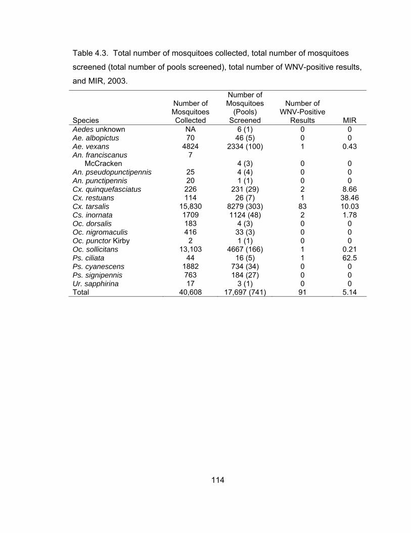
Table 4.3. Total number of mosquitoes collected, total number of mosquitoes
screened (total number of pools screened), total number of WNV-positive results,
and MIR, 2003.
Species
Number of Mosquitoes Collected
Number of Mosquitoes
(Pools) Screened
Number of WNV-Positive
Results MIR Aedes unknown NA 6 (1) 0 0 Ae. albopictus 70 46 (5) 0 0 Ae. vexans 4824 2334 (100) 1 0.43 An. franciscanus
McCracken 7
4 (3) 0 0 An. pseudopunctipennis 25 4 (4) 0 0 An. punctipennis 20 1 (1) 0 0 Cx. quinquefasciatus 226 231 (29) 2 8.66 Cx. restuans 114 26 (7) 1 38.46 Cx. tarsalis 15,830 8279 (303) 83 10.03 Cs. inornata 1709 1124 (48) 2 1.78 Oc. dorsalis 183 4 (3) 0 0 Oc. nigromaculis 416 33 (3) 0 0 Oc. punctor Kirby 2 1 (1) 0 0 Oc. sollicitans 13,103 4667 (166) 1 0.21 Ps. ciliata 44 16 (5) 1 62.5 Ps. cyanescens 1882 734 (34) 0 0 Ps. signipennis 763 184 (27) 0 0 Ur. sapphirina 17 3 (1) 0 0 Total 40,608 17,697 (741) 91 5.14
114
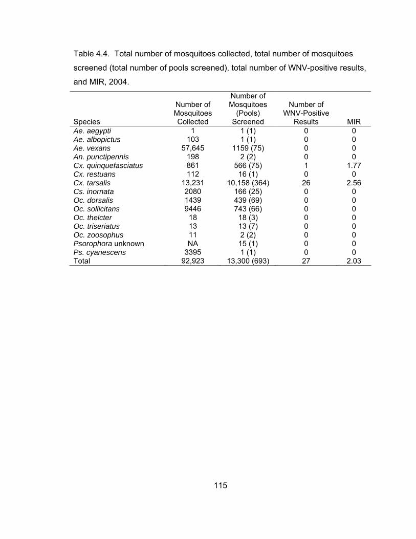
Table 4.4. Total number of mosquitoes collected, total number of mosquitoes
screened (total number of pools screened), total number of WNV-positive results,
and MIR, 2004.
Species
Number of Mosquitoes Collected
Number of Mosquitoes
(Pools) Screened
Number of WNV-Positive
Results MIR Ae. aegypti 1 1 (1) 0 0 Ae. albopictus 103 1 (1) 0 0 Ae. vexans 57,645 1159 (75) 0 0 An. punctipennis 198 2 (2) 0 0 Cx. quinquefasciatus 861 566 (75) 1 1.77 Cx. restuans 112 16 (1) 0 0 Cx. tarsalis 13,231 10,158 (364) 26 2.56 Cs. inornata 2080 166 (25) 0 0 Oc. dorsalis 1439 439 (69) 0 0 Oc. sollicitans 9446 743 (66) 0 0 Oc. thelcter 18 18 (3) 0 0 Oc. triseriatus 13 13 (7) 0 0 Oc. zoosophus 11 2 (2) 0 0 Psorophora unknown NA 15 (1) 0 0 Ps. cyanescens 3395 1 (1) 0 0 Total 92,923 13,300 (693) 27 2.03
115

Figure 4.8. Total number of WNV-positive mosquito pools by week, 2002
through 2004.
Over the course of this study, almost 33,000 mosquitoes (1509 pools)
were screened for WNV, and 121 pools of mosquitoes tested positive for the
disease. Of these 121 positive tests, all but 10 were pools of Cx. tarsalis, and
four of these 10 were other Culex species. The remaining six positive pools were
Ae. vexans (2), Cs. inornata (2), Oc. sollicitans (1), and Ps. ciliata (1). Although
screening was sporadic in 2002 when surveillance operations were initiated, the
first WNV-positive pools were detected late that summer and early fall [87]. The
year in which Lubbock County had the highest number of WNV-positive
mosquitoes was 2003, in which 91 pools of mosquitoes tested positive. Most of
these positive pools were collected during July, August, and September, with a
few positive pools appearing later in the fall. The following year, the number of
WNV-positive mosquito pools was greatly reduced, despite approximately the
116

same number of pools being tested. The 27 positive pools occurred slightly later
than in 2003.
As the majority of the WNV-positive pools consisted of Cx. tarsalis,
analyses of WNV maintenance and transmission were conducted using the
number of Cx. tarsalis collected per trap-night in addition to the total number of
mosquitoes collected per trap-night. Also, since mosquito screening for WNV
was sporadic in 2002, only data from 2003 and 2004 are analyzed. Smoothing
spline transformations were used to obtain a view of relationships among
weather conditions, mosquito collections, and WNV occurrence. Figures 4.9
through 4.22 illustrate these relationships.
Figure 4.9. Weekly MIR in relation to the smoothing spline transformation of
average weekly air temperature (°C), 2003.
117

Figure 4.10. Weekly MIR in relation to the smoothing spline transformation of
average weekly relative humidity (%), 2003.
Figure 4.11. Weekly MIR in relation to total weekly precipitation (mm), 2003.
118

Figure 4.12. Weekly MIR in relation to the smoothing spline transformation of
total weekly heat units, 2003.
Figure 4.13. Weekly MIR in relation to the smoothing spline transformation of
cumulative heat units, 2003.
119

Figure 4.14. Weekly MIR in relation to the smoothing spline transformation of
total number of mosquitoes collected per trap-night, 2003.
Figure 4.15. Weekly MIR in relation to the smoothing spline transformation of
total number of Cx. tarsalis collected per trap-night, 2003.
120
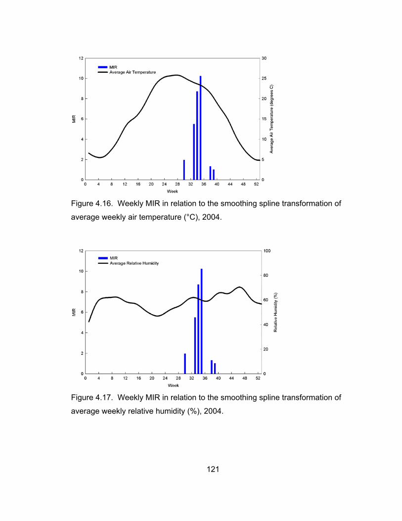
Figure 4.16. Weekly MIR in relation to the smoothing spline transformation of
average weekly air temperature (°C), 2004.
Figure 4.17. Weekly MIR in relation to the smoothing spline transformation of
average weekly relative humidity (%), 2004.
121

Figure 4.18. Weekly MIR in relation to total weekly precipitation (mm), 2004.
Figure 4.19. Weekly MIR in relation to the smoothing spline transformation of
total weekly heat units, 2004.
122

Figure 4.20. Weekly MIR in relation to the smoothing spline transformation of
cumulative heat units, 2004.
Figure 4.21. Weekly MIR in relation to the smoothing spline transformation of
total number of mosquitoes collected per trap-night, 2004.
123
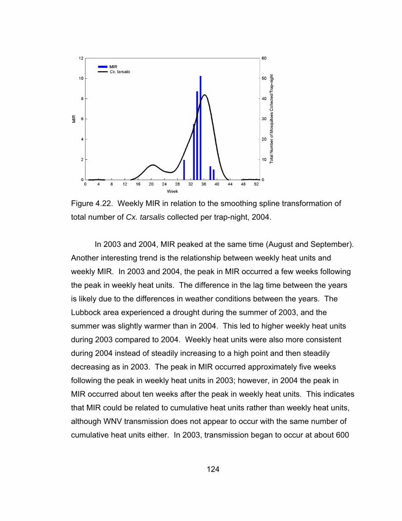
Figure 4.22. Weekly MIR in relation to the smoothing spline transformation of
total number of Cx. tarsalis collected per trap-night, 2004.
In 2003 and 2004, MIR peaked at the same time (August and September).
Another interesting trend is the relationship between weekly heat units and
weekly MIR. In 2003 and 2004, the peak in MIR occurred a few weeks following
the peak in weekly heat units. The difference in the lag time between the years
is likely due to the differences in weather conditions between the years. The
Lubbock area experienced a drought during the summer of 2003, and the
summer was slightly warmer than in 2004. This led to higher weekly heat units
during 2003 compared to 2004. Weekly heat units were also more consistent
during 2004 instead of steadily increasing to a high point and then steadily
decreasing as in 2003. The peak in MIR occurred approximately five weeks
following the peak in weekly heat units in 2003; however, in 2004 the peak in
MIR occurred about ten weeks after the peak in weekly heat units. This indicates
that MIR could be related to cumulative heat units rather than weekly heat units,
although WNV transmission does not appear to occur with the same number of
cumulative heat units either. In 2003, transmission began to occur at about 600
124

cumulative heat units, whereas in 2004 transmission began to occur at about 800
cumulative heat units. In both years, MIR peaked at around 1200 cumulative
heat units for the year. Transmission of WNV in response to rainfall also varied
between the years, with transmission peaking about eight weeks following heavy
rainfall in 2003 but about five weeks before heavy rainfall in 2004.
Trends in MIR in relation to number of Cx. tarsalis collected per trap-night
and total number of mosquitoes collected per trap-night were also variable.
During 2003, when half of the mosquitoes collected per trap-night were Cx.
tarsalis, the peak in MIR occurred about four weeks after the peak in Cx. tarsalis
populations and six weeks after the peak in total number of mosquitoes collected
per trap-night. Conversely, in 2004, when most of the mosquitoes collected were
Ae. vexans, the MIR peak occurred about two weeks prior to the peak in Cx.
tarsalis populations and eight weeks prior to the peak in total number of
mosquitoes collected. The lack of relationship between total number of
mosquitoes collected per trap-night and MIR in 2004 is not surprising since only
two pools of Ae. vexans tested positive for WNV throughout the study. The
relationship between Cx. tarsalis populations and MIR during 2004 is interesting
in that the Cx. tarsalis smoothing spline appears to directly shadow the MIR
smoothing spline.
When only weather conditions were used to model MIR, the best one-
variable regression model (using the maximum r2 improvement technique)
included a lag in the total number of weekly heat units. For 2003, this term
included the total number of heat units two to five weeks prior to collection
whereas in 2004 it was four to eight weeks prior to collection (r2=0.7841 and
0.4893, respectively), which follows the trends seen in the figures above. The
best two-variable model for MIR in 2003 included the average relative humidity
four to eight weeks prior to collection in addition to the lag in total heat units
(r2=0.9221). In 2004, the average air temperature and total heat units four to
eight weeks prior to collection were the best indicators of MIR (r2=0.5916). See
125

Tables 4.5 and 4.6 for complete model parameter estimates for the best models
containing one to five parameters.
Table 4.5. Best models for MIR based upon weather conditions only, 2003. All
models were highly significant (p<0.0001). Model
r2
Variable Coefficient Standard
Error
p-value
0.7841 Intercept -3.35612 0.90391 0.0009
Total heat units, 2 to 5 wk prior to collection 0.04051 0.00402 < 0.0001
0.9221 Intercept -15.65868 1.84289 < 0.0001
Average relative humidity, 4 to 8 wk prior to collection 0.23791 0.03381 < 0.0001
Total heat units, 3 to 4 wk prior to collection 0.08779 0.00499 < 0.0001
0.9621 Intercept -8.43330 1.70454 < 0.0001
Average relative humidity, 1 to 5 wk prior to collection -0.18838 0.03069 < 0.0001
Average relative humidity, 4 to 8 wk prior to collection 0.28678 0.02607 < 0.0001
Total heat units, 2 to 6 wk prior to collection 0.03440 0.00150 < 0.0001
0.9654 Intercept -3.59788 3.56928 0.3231
Average air temperature, 2 to 6 wk prior to collection -0.38280 0.25006 0.1384
Average relative humidity, 1 to 5 wk prior to collection -0.17300 0.03157 < 0.0001
Average relative humidity, 4 to 8 wk prior to collection 0.27565 0.02644 < 0.0001
Total heat units, 2 to 6 wk prior to collection 0.04806 0.00904 < 0.0001
0.9667 Intercept -3.71896 3.57556 0.3087
Average air temperature, 2 to 6 wk prior to collection -0.47219 0.26674 0.0894
Average relative humidity, 1 to 5 wk prior to collection -0.17017 0.03174 < 0.0001
Average relative humidity, 4 to 8 wk prior to collection 0.29439 0.03276 < 0.0001
Total heat units, 2 to 6 wk prior to collection 0.05168 0.00979 < 0.0001
Total rainfall, week of collection 0.02425 0.02498 0.3413
126
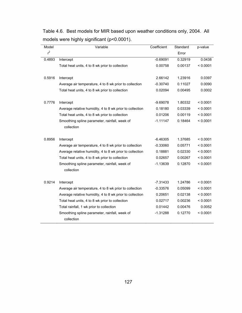
Table 4.6. Best models for MIR based upon weather conditions only, 2004. All
models were highly significant (p<0.0001). Model
r2
Variable Coefficient Standard
Error
p-value
0.4893 Intercept -0.69091 0.32919 0.0438
Total heat units, 4 to 8 wk prior to collection 0.00758 0.00137 < 0.0001
0.5916 Intercept 2.66142 1.23916 0.0397
Average air temperature, 4 to 8 wk prior to collection -0.30740 0.11027 0.0090
Total heat units, 4 to 8 wk prior to collection 0.02094 0.00495 0.0002
0.7776 Intercept -9.69078 1.80332 < 0.0001
Average relative humidity, 4 to 8 wk prior to collection 0.18180 0.03339 < 0.0001
Total heat units, 4 to 8 wk prior to collection 0.01206 0.00119 < 0.0001
Smoothing spline parameter, rainfall, week of
collection
-1.11147 0.18464 < 0.0001
0.8956 Intercept -6.46305 1.37685 < 0.0001
Average air temperature, 4 to 8 wk prior to collection -0.33060 0.05771 < 0.0001
Average relative humidity, 4 to 8 wk prior to collection 0.18881 0.02330 < 0.0001
Total heat units, 4 to 8 wk prior to collection 0.02657 0.00267 < 0.0001
Smoothing spline parameter, rainfall, week of
collection
-1.13639 0.12870 < 0.0001
0.9214 Intercept -7.31433 1.24786 < 0.0001
Average air temperature, 4 to 8 wk prior to collection -0.33576 0.05099 < 0.0001
Average relative humidity, 4 to 8 wk prior to collection 0.20651 0.02138 < 0.0001
Total heat units, 4 to 8 wk prior to collection 0.02717 0.00236 < 0.0001
Total rainfall, 1 wk prior to collection 0.01442 0.00476 0.0052
Smoothing spline parameter, rainfall, week of
collection
-1.31288 0.12770 < 0.0001
127

With the addition of variables for number of Cx. tarsalis collected per trap-
night and total number of mosquitoes collected per trap-night, the best models
including one to five variables for 2003 did not change, and the parameter for Cx.
tarsalis populations was not entered into the model until a 27-variable model was
used to explain MIR. Additionally, the total number of mosquitoes collected per
trap-night was never entered into the model, indicating that these terms were not
important in explaining WNV that year. In 2004, however, when these terms
were added to the analysis, the best one-variable model for MIR was the total
number of Cx. tarsalis collected per trap-night in the current week (r2=0.8027).
The best two-variable model included the average relative humidity in the two
weeks prior to collection in addition to the total number of Cx. tarsalis collected
per trap-night in the current week (r2=0.8241). See Tables 4.7 and 4.8 for
complete model parameter estimates for the best models containing one to five
parameters.
128

Table 4.7. Best models for MIR based upon weather conditions and vector
abundance, 2003. Collection refers to the collection of WNV-positive
mosquitoes. All models were highly significant (p<0.0001). Model
r2
Variable Coefficient Standard
Error
p-value
0.7841 Intercept -3.35612 0.90391 0.0009
Total heat units, 2 to 5 weeks prior to collection 0.04051 0.00402 < 0.0001
0.9221 Intercept -15.65868 1.84289 < 0.0001
Average relative humidity, 4 to 8 wk prior to collection 0.23791 0.03381 < 0.0001
Total heat units, 3 to 4 wk prior to collection 0.08779 0.00499 < 0.0001
0.9621 Intercept -8.43330 1.70454 < 0.0001
Average relative humidity, 1 to 5 wk prior to collection -0.18838 0.03069 < 0.0001
Average relative humidity, 4 to 8 wk prior to collection 0.28678 0.02607 < 0.0001
Total heat units, 2 to 6 wk prior to collection 0.03440 0.00150 < 0.0001
0.9654 Intercept -3.59788 3.56928 0.3231
Average air temperature, 2 to 6 wk prior to collection -0.38280 0.25006 0.1384
Average relative humidity, 1 to 5 wk prior to collection -0.17300 0.03157 < 0.0001
Average relative humidity, 4 to 8 wk prior to collection 0.27565 0.02644 < 0.0001
Total heat units, 2 to 6 wk prior to collection 0.04806 0.00904 < 0.0001
0.9667 Intercept -3.71896 3.57556 0.3087
Average air temperature, 2 to 6 wk prior to collection -0.47219 0.26674 0.0894
Average relative humidity, 1 to 5 wk prior to collection -0.17017 0.03174 < 0.0001
Average relative humidity, 4 to 8 wk prior to collection 0.29439 0.03276 < 0.0001
Total heat units, 2 to 6 wk prior to collection 0.05168 0.00979 < 0.0001
Total rainfall, week of collection 0.02425 0.02498 0.3413
129

Table 4.8. Best models for MIR based upon weather conditions and vector
abundance, 2004. Collection refers to the collection of WNV-positive
mosquitoes. Number of Cx. tarsalis collected refers to the number of Cx. tarsalis
collected per trap-night. All models were highly significant (p<0.0001). Model
r2
Variable Coefficient Standard
Error
p-value
0.8027 Intercept -0.26549 0.14684 0.0800
Number of Cx. tarsalis collected, week of collection 0.09785 0.00858 < 0.001
0.8241 Intercept -1.60350 0.70233 0.0294
Average relative humidity, 1 to 2 wk prior to collection 0.02405 0.01237 0.0609
Number of Cx. tarsalis collected, week of collection 0.09541 0.00832 < 0.0001
0.8591 Intercept 8.79496 2.69791 0.0028
Average relative humidity, 4 to 8 wk prior to collection -0.11712 0.03390 0.0017
Number of Cx. tarsalis collected, week of collection 0.11758 0.01018 < 0.0001
Smoothing spline parameter, average air
temperature, week of collection
-0.12813 0.04537 0.0083
0.8776 Intercept 3.60434 1.49869 0.0228
Total rainfall, 1 to 4 wk prior to collection 0.01049 0.00293 0.0012
Number of Cx. tarsalis collected, week of collection 0.11104 0.00869 < 0.0001
Smoothing spline parameter, average air
temperature, week of collection
-0.38549 0.12282 0.0039
Smoothing spline parameter, heat units, week of
collection
0.55850 0.16282 0.0018
0.9700 Intercept -9.57297 0.79640 < 0.0001
Total heat units, 3 to 4 wk prior to collection -0.00579 0.00167 0.0017
Total rainfall, 3 to 7 wk prior to collection -0.01375 0.00234 < 0.0001
Number of Cx. tarsalis collected, week of collection 0.07684 0.00448 < 0.0001
Smoothing spline parameter, average relative
humidity, week of collection
0.23696 0.02058 < 0.0001
Smoothing spline parameter, rainfall, week of
collection
-1.38502 0.11898 < 0.0001
130

Many mosquito-borne diseases are endemic throughout areas of the
United States, and surveillance for these diseases typically involves the
collection and screening of mosquitoes for various arboviruses, followed by
retrospective attempts to understand why and how transmission occurred in
certain patterns. Only by understanding the dynamics of disease transmission
can effective and proactive vector control strategies by undertaken. Many
studies have shown that weather, and especially anomalous weather, is a major
contributor to the occurrence and persistence of mosquito-borne diseases.
Prior to the outbreak of WNV, arboviruses of concern in California
included WEE and SLE [67]. State-wide surveillance for these diseases had
indicated a general decline in the incidence of these diseases since 1970 in the
Central Valley, while viral activity had been consistent in Coachella and Imperial
Valleys since 1967. Whereas mosquito abundance peaked at approximately
25°C, viral activity tended to occur when temperatures exceeded 29°C. Culex
tarsalis populations peaked twice in a given year, once in the spring and once in
the fall. In these populations, WEE was detected just after the spring peak and
SLE was detected just before the fall peak of Cx. tarsalis [67]. Continued
surveillance for WEE and SLE in California has shown that viral transmission
was directly related to Cx. tarsalis populations, which were related to the
availability of larval habitats during spring and late summer [63, 106].
Although this describes the behavior of two different arboviruses, a similar
pattern was observed in the relationship of WNV and Cx. tarsalis populations in
Lubbock. In 2003, WNV was detected in Cx. tarsalis populations just after the
spring peak in abundance, as seen in WEE in California. The next year,
however, heavy rainfall throughout the spring and summer eliminated suitable
habitats for Cx. tarsalis development and the spring peak in abundance was
shifted to a fall peak in abundance. Mosquitoes testing positive for WNV then
appeared just before the fall peak in Cx. tarsalis abundance, as seen for SLE in
California.
131

Andreadis and others [107] found that hot, dry summers provided suitable
habitats for the proliferation of Cx. pipiens, one of the major vectors of WNV in
Connecticut. Increased populations of this vector species led to highly
concentrated foci of viral activity in urban areas. Based upon this, it was
predicted that wet summers would increase the abundance of other potential
vector species and more widespread viral activity [107]. In Rhode Island, above-
average rainfall during 1996 and 1998 led to increased arboviral activity (EEE
and Highlands J virus). Although more mosquitoes were collected during 1997,
mosquito abundance during these two years were also increased. However, the
Takeda and others study does not describe the species of mosquitoes that were
collected, except to mention that Coquillettidia perturbans was the most
abundant (21%) species collected throughout the study [108].
A similar phenomenon was observed in Australia when above-average
rainfall led to a population explosion of Oc. vigilax Skuse, followed by the largest
recorded outbreak of human disease involving Burmah Forest virus eight weeks
later [65]. Historically, Rift Valley fever virus outbreaks in Kenya occur when
periods of heavy rainfall flood breeding areas of Aedes spp. [109]. Ross River
virus epidemics in Australia are also predicted based upon timing, duration, and
extent of rainfall, with heavy rainfall producing Culex mosquitoes [110].
As rainfall influences transmission of mosquito-borne diseases, drought is
also known to influence transmission and distribution of SLE [111, 112]. Florida
is prone to outbreaks of SLE, and variations in water table depth can be used to
predict abundance of Cx. nigripalpus (major vector of SLE) as well as SLE
transmission. Dynamic hydrology models have shown that droughts during the
spring restrict the distribution of Cx. nigripalpus to forested areas above marshes,
which are also areas occupied by wild birds (nestling, juvenile, and adult), a
situation that creates the perfect setting for rapid amplification of SLE. As the
droughts end, dispersal of infected mosquitoes and birds from these hammocks
into new aquatic habitats facilitates the transmission of SLE [111, 112].
132

Throughout the United States, 10 of the 12 urban outbreaks of SLE during 1933
through 1974 were associated with at least two prior months of consecutive
drought [113].
Similarly, drought conditions may be useful in predicting WNV
transmission. Worldwide, major outbreaks of WNV have followed prolonged
drought in Israel (1951), Romania (1996), and Russia (1999) [113]. The first
appearance of WNV in the United States in New York City also coincided with a
severe drought during spring and summer months in that year [113]. Studies of
WNV in Florida produced similar results as those of SLE in Florida, in that
periods of spring drought brought vector and host populations into close contact,
allowing for WNV amplification, and rainfall during the summer and fall allowed
for the migration of these vector and host populations to new habitats and
facilitated transmission of WNV to naïve vectors and hosts. Interesting to note is
that Florida has not had a significant drought since WNV was introduced into that
state in 2001. The state also has not experienced a major WNV epidemic [114].
Although the Shaman and others study related lack of a significant drought in
Florida with lack of a major WNV epidemic, evaluations of mosquito control
programs throughout the state were not included, so this conclusion is somewhat
suspect.
Drought-induced amplification may also be used to describe WNV activity
in the Lubbock area during 2003. Drought conditions during the late winter
through spring of 2003 reduced the availability of aquatic habitats for mosquitoes
and birds; thus the few remaining bodies of water were likely occupied by large
numbers of vector and host populations. Late spring rains refreshed playas and
drainage basins throughout the county, and populations dispersed. Further
drought conditions during the summer allowed for the proliferation of Cx. tarsalis
as well as maintenance and transmission of WNV. Late fall rains were also
followed by a small peak in WNV occurrence.
133

Mosquito-borne diseases are not the only zoonoses that are affected by
weather conditions, and of the many examples that are available, only a few are
mentioned here for comparison. Lyme disease risk is indirectly associated with
weather conditions in that weather changes the ecology of the mammalian host
communities [115]. Frequency of human plague cases has been modeled using
maximum daily summer temperatures and time-lagged amounts of late winter
precipitation, with close agreement between predicted and observed number of
cases [116]. During 1998 and 1999, increased incidence of Q fever, a zoonosis
that is transmitted by the inhalation of infected aerosols from mammals, was
linked to increased winds following the lambing season [117].
Conclusions and Future Studies
West Nile virus first emerged in Lubbock, TX, in the summer of 2002, and
epidemics have occurred each summer since then. The dominant vector of WNV
in the Lubbock area was Cx. tarsalis, with 111 of the 121 WNV-positive pools
being of this species. The summer and early fall of 2003 had the highest number
of WNV-positive pools, likely due to an increase in the vector population due to
drought conditions. Relationships among the weekly infection rate of WNV and
weather as well as collections of Cx. tarsalis were apparent in both graphical
displays as well as regression analyses. During the drought year of 2003, MIR
was explained by relative humidity and heat units during the two months prior to
the collection of WNV-positive mosquitoes. Models of MIR did not change with
the addition of variables for mosquito collections. During 2004, when weather
alone was used to explain MIR, variables included a combination of all the
weather variables; however, when a variables for collections of Cx. tarsalis was
added to the model, it was a strong indicator of weekly MIR. Future studies will
involve the continued surveillance for WNV in Lubbock and the surrounding
areas in an effort to improve and standardize models for predicting WNV
occurrence (Chapter VI).
134

CHAPTER V
PRELIMINARY STUDIES ON THE EFFECTS OF PESTICIDES ON MOSQUITO
COMMUNITIES AND WEST NILE VIRUS MAINTENANCE AND
TRANSMISSION
Introduction and Research Goals
Traditional mosquito control strategies rely on larvicides to prevent the
emergence of adult mosquitoes, adulticides to control mature mosquitoes,
physical prevention mechanisms such as breeding site reduction, window
screens, and individual personal protection against mosquito feeding, or any
combination of these [118]. Larvicides are more effective than adulticides but
require accurate application to minimize non-target effects on other organisms as
well as continued surveillance to determine efficacy of treatment. Larvicides
include organophosphate pesticides such as temephos (Abate®), biological
larvicides such as Bacillus thuringiensis israelensis (Bti), insect growth regulators
such as methoprene (Altosid®), and a variety of oils and surface films that disrupt
water surface tension and drown larvae and pupae [119]. Biological control
through the use of predaceous fish such as Gambusia provides some degree of
larvae control in semipermanent to permanent water bodies. Adulticides are
typically used to quickly reduce mosquito abundance, especially when there is a
risk of disease transmission. Although they typically do not pose health risks to
humans and wildlife if used correctly, their effectiveness requires direct
application throughout areas where adult mosquitoes are flying [119].
Insecticides labeled for use as adulticides include organophosphates such as
malathion (Fyfanon®) and synthetic pyrethroids such as permethrin
(Permanone®). Although these methods are effective, source reduction by
limiting or altering mosquito breeding sites is the most effective and economical
means for long-term control of mosquitoes [119].
135

Application of insecticides for control of adult mosquitoes is typically
conducted using ultra-low volume (ULV) application with ground equipment. This
type of pesticide application disperses less than 2 L of pesticide per acre, using
droplet sizes of 5 to 27 µm [44]. Thermal fogging, an older method of adult
mosquito control, requires the addition of a fuel oil carrier and a high temperature
system to produce fog droplets. Thermal fogging and ULV applications are
similar in their effectiveness [44]. Adult mosquito control is considered a
temporary means of mosquito control, as mosquitoes from areas that are not
sprayed can quickly move into areas that have previously been sprayed.
Additionally, application of insecticides for adult control are not effective against
immature stages [44].
With the growing number of emerging and resurgent arthropod-transmitted
diseases as discussed in Chapter I, the importance of vector control is increasing
in importance and focus. Typically, mosquito control operations take place in
urban and suburban areas, whereas agricultural pest control operations take
place on croplands in rural areas. However, in many areas, neighborhoods are
encroaching into these croplands resulting in an overlap between residential and
agricultural areas. It is important to look at these semi-rural and suburban areas
that occur at the urban-rural interface to determine whether agricultural pest
control efforts have any effects upon biota that exist at this interface and
especially upon mosquito community dynamics. Therefore, the objective of this
portion of the research project was to evaluate and determine appropriate
strategies for determining the indirect effects of agricultural crop spraying with
insecticides on mosquito abundance and ultimately on WNV occurrence. This
was accomplished using local mosquito control adulticide applications as a
model to develop methods for measuring efficacy and drift of applied agricultural
crop pesticides.
136

Materials and Methods
The City of Lubbock and Texas Tech University were contacted to
determine what insecticide(s) were being used for mosquito control in the
Lubbock area. Local commercial aerial agricultural crop applicators were also
contacted to determine which insecticides were used on crops such as cotton for
insect control. Pesticide applicators agreed to provide advanced notice as to
when spraying would be conducted. Due to weather restraints that prevented
aerial applications of pesticides on agricultural crops, this portion of the study
was not completed.
Texas Tech University used Fyfanon® (malathion) in thermal foggers for
mosquito control on the Texas Tech University campus, so malathion (in the form
of Fyfanon®) was purchased from Cheminova, Inc. (Wayne, NJ) for use as a
standard and consisted of 96 to 97% malathion. The City of Lubbock used
Permanone® (permethrin, Bayer Environmental Science, Montvale, NJ) in ULV
sprayers for mosquito control throughout Lubbock County (33.65°N; 101.81°W;
975 m elevation). A permethrin standard was purchased from ChemService, Inc.
(West Chester, PA) at a concentration of 100 µg/ml.
The method developed and tested involved using an experimental grid,
with a cage containing approximately 50 live adult mosquitoes placed in the
center of the grid and then placing stakes 30.48 m north, south, east, and west of
this cage. On top of each stake and on each cage filter papers were placed to
collect droplets from the pesticide application (Figure 5.1). In addition, mosquito
light traps were operated and mosquitoes collected at the experimental location
on the night prior to and the night after insecticide application to determine if
there were differences in the number of mosquitoes collected and in the species
composition.
137

Figure 5.1. Stake (left) and mosquito cage containing live mosquitoes (right) with
sample papers attached to the top for collection of residues from mosquito
control pesticide applications.
Within six hours following pesticide application, the filter papers were
collected and analyzed according to the methods described below. The number
of surviving caged mosquitoes was also determined. For the second set of
experimental locations described below, the grid was expanded by adding stakes
60.96 m north, south, east, and west of the cage as well as 30.48 m northeast,
northwest, southeast, and southwest from the cage to obtain more data
regarding insecticide drift.
For this study, several experimental locations were set up to evaluate the
experimental design. Three sites in addition to a control site were set up during
one night of permethrin spraying by the City of Lubbock. Due to lack of
advanced notice, mosquito trapping was not conducted on the night prior to and
post spraying. All three experimental grids were on the property where mosquito
spraying was to be conducted, but ranged in distance from where the plume
138

would originate (near, mid-distance, and far). The control site was set up in an
area where spraying was not to be conducted that night. On another occasion,
two experimental sites and a control were set up for a night of malathion spraying
by Texas Tech University. Mosquitoes were trapped at the two experimental
locations on the night before spraying, but due to low collection numbers, were
not trapped on the night after spraying. Again, the control site was set up in an
area where no spraying was to be conducted.
Insecticidal residues on sample papers were extracted by mechanical
agitation using 15 ml of hexane on a shaker (120 rpm) for 20 minutes. This
procedure was repeated and the extracts were pooled. Since there was no
evidence of interference from other substances, there was no clean-up
procedure prior to analysis. Extracts were analyzed using a Hewlett-Packard
6890 Gas Chromatograph (Hewlett-Packard Company, Wilmington, DE).
Samples containing permethrin were analyzed using an electron capture
detector, and samples containing malathion were analyzed using a flame
photometric detector in the phosphorous mode.
In addition, a separate set of sample papers were spiked with either 0.5
mg/L of malathion or permethrin and were set outside for up to 12 hours to
determine chemical stability under environmental conditions. Permethrin was
stable under environmental conditions for up to 12 hours and malathion was
stable under environmental conditions for up to eight hours, followed by a rapid
drop in concentration (Figure 5.2).
139

Figure 5.2. Stability of permethrin and malathion under environmental conditions
from 0 to 12 hours (one sample per time period analyzed). Sample papers were
spiked with 0.5 mg/L of malathion or permethrin.
Results and Discussion
No permethrin was detected in samples from two of the three test
locations or at the control location following pesticide application by the City of
Lubbock, but there was a higher percentage of caged mosquito mortality at these
locations compared to only about 50% mortality at the control location. Small
permethrin peaks were detected in three samples at the experimental location
that was set up near the origin of spaying, but these could not be quantified.
Also at this location, there was 100% mortality of caged mosquitoes.
Malathion was detected in samples from both test locations during
pesticide application by Texas Tech University but not at the control location. At
experimental location one, malathion was detected in only two samples, with a
higher concentration of pesticide in the sample paper located 30.48 m north of
the cage. At experimental location two, malathion was detected in all samples,
140

but the highest concentrations were found in the two samples closest to the
spraying route. This insecticide drift also corresponded to the wind direction and
speed (7 m/s northeast) during the malathion application. See Figures 5.3 and
5.4 for more detail.
Figure 5.3. Malathion experimental location one with expanded experimental
grid. Malathion was detected in the two samples indicated (circled). The sample
indicated in green had a concentration of ~0.108 µg/paper and the sample
indicated in pink had a concentration of ~0.0066 µg/paper. The spraying route is
indicated by the red line and wind speed and direction by the blue arrow.
141

7 m/s7 m/s7 m/s
Figure 5.4. Malathion experimental location two. Malathion was detected in all
samples from this area, and there was a higher percentage of mortality (~75%) of
caged mosquitoes than at location one or the control (~50%). The sample
indicated in green had a concentration of ~0.031 µg/paper and the sample
indicated in pink had a concentration of ~0.022 µg/paper. The spraying route is
indicated by the red line and wind by the blue arrow.
Conclusions and Future Studies
Although wind speed at the time of pesticide application was just above
that of the recommended range, pesticide residues were detected in sample
papers, indicating that the experimental grid design proposed in this study is a
useful method for monitoring drift from mosquito control applications and
evaluating the efficacy of pesticide delivery by ULV and thermal fogging. Future
studies will involve improving this method and applying the experimental grid
design during agricultural crop spraying and to determine the effects of
agricultural crop spraying on mosquito communities (Chapter VI).
142

CHAPTER VI
CONCLUSIONS AND FUTURE RESEARCH
Study Summary and Conclusions
Emerging and resurgent vector-borne diseases have recently come into
the spotlight, especially with the concerns of potential global climate change and
biologic attacks. One of these emerging vector-borne diseases is West Nile virus
(WNV), which first appeared in the United States in the summer of 1999 and
quickly spread across the entire continental United States. Despite increased
surveillance and control operations, WNV continues to be a threat to humans,
domestic animals, wildlife, and particularly horses.
The goal of this project was to determine the factors involved in the
emergence of WNV in an area, in an attempt to model how these factors
influence WNV maintenance and transmission. Understanding how weather
conditions and landscape features influence mosquito community dynamics and
ultimately WNV transmission is critical for effective surveillance and control
programs. Additionally, models of disease transmission can be used to predict
future outbreaks of disease, and appropriate control strategies can be initiated to
try to prevent devastating epidemics. Models of disease transmission are also
useful for differentiating between a naturally occurring outbreak of disease and
an act of terrorism using biological weapons. It was hypothesized that weather
conditions, especially rainfall, in the weeks prior to mosquito collection would
influence mosquito community dynamics, and that collections of vector species
would influence occurrence of WNV.
Mosquito surveillance was initiated in Lubbock County, TX, during the
summer of 2002. Surveillance operations included collecting mosquitoes using a
variety of trap types and screening them for WNV using reverse-transcriptase
polymerase chain reaction and the VecTest® Antigen Assay. West Nile virus was
first detected in Lubbock, TX, during 2002, and viral occurrence has been
143

documented every summer since then. Mosquito collections from 2002 through
2004 were related to weather conditions and trapping site profiles in order to
determine how these influence mosquito community dynamics. Additionally,
WNV occurrence in mosquitoes was modeled using weather conditions and
mosquito abundance.
The three-year study period was ideal in that observations of mosquito
communities and WNV transmission were made over an average year (2002), an
extremely dry year (2003), and an extremely wet year (2004). During 2003, the
dominant mosquito species collected in Lubbock, TX, was Culex tarsalis
Coquillett, whereas in 2004 the dominant species was Aedes vexans Meigen.
Mosquito collections were dependent both upon mosquito trapping site profiles
and weather conditions in the weeks prior to collection. Based upon subjective
evaluation of mosquito trapping locations, landscape features that influenced
mosquito abundance included vegetation and potential breeding sites. Weather
conditions influencing mosquito communities included rainfall and heat units in
the four to eight weeks prior to mosquito collection. Culex tarsalis was the main
vector of WNV in the Lubbock area, with 111 of the 121 WNV-positive pools
being of this species. During 2003, the number of WNV-positive mosquito pools
was much higher, despite approximately the same number of pools being
screened during 2004. This phenomenon was likely due to drought conditions
during 2003 that encouraged the proliferation of Cx. tarsalis. The weekly
infection rate of WNV was explained based upon weather conditions and vector
abundance; however, models of infection rate were significantly different
between 2003 and 2004, likely due to diverse weather conditions.
There were interactions seen between rare events (flood and drought) and
mosquito community dynamics as well as WNV maintenance and transmission.
The population explosion of Ae. vexans was only seen during a flood year.
Additionally, Cx. tarsalis dominance and high WNV maintenance and
transmission were limited to a drought year. This indicates that rare events may
144

have a significant impact on models of disease transmission. However, since
there was only one year of average weather and two years of rare weather on
opposite ends of the precipitation scale (dry and wet), continued disease
surveillance will allow for the validation and improvement of disease models
designed in the present study.
In addition to modeling factors involved in mosquito abundance and WNV
occurrence, an additional study was conducted to develop a procedure for
determining the influence of agricultural pesticides on mosquito abundance and
ultimately upon WNV occurrence. The City of Lubbock is an agricultural
community, with residential areas encroaching into agricultural areas. Insecticide
application for mosquito control was used as a model for method development,
and insecticide residues were detected from samples collected at or near the
route traveled during mosquito control operations. The concentrations of these
residues were related to both the chemical applicator’s driving route and the wind
direction during spraying. Results of this study indicated the use of an
experimental grid was effective in determining the drift from pesticide application,
as well as for evaluating the efficacy of mosquito control operations.
Future Studies to Address New Questions
The results of this project indicate that there are many avenues that may
be pursued for future research. Although good models for mosquito community
dynamics and WNV occurrence were produced, continued surveillance over a
longer time period will allow for the improvement of these models as well as
potentially create acceptable models despite variable weather. Differences in
models were apparent between a wet year and a dry year, and so data collected
over a longer time period may help average some of these differences.
Surveillance of mosquito communities is necessary to monitor how
species composition changes over time, with the introduction of new mosquito
species and the loss of historic species, as potential climate change may result in
145

changes in the distribution of various mosquito species. Additionally, there are a
number of studies that may be conducted to evaluate other factors that might be
involved in mosquito community dynamics. In this study, mosquito communities
were related to weather conditions at a central location in the Lubbock area.
However, weather conditions across the South Plains are highly variable, and
weather conditions at different trapping sites may be variable. Thus, evaluating
the microclimate using individual weather data recorders at each trapping site
may aid in determining how weather influences mosquito populations on a more
localized scale. Additionally in this study, landscape features at each trapping
site were not quantified; rather, general characterizations were used. Future
studies should involve quantifying landscape features at each site to better
understand how these features affect mosquito populations. Trapping sites may
be evaluated by assigning them to different categories (such as open field,
residential area, playa) and then using canonical correspondence analysis to
determine the extent of variation in mosquito that may be explained by these
variables [120, 121]. Additionally, remote sensing and geographic information
systems technologies may be applied to map trapping sites, and regression
analysis (similar to that which was done for the weather data in this study) can be
used to determine how vegetation and other features influence mosquito
populations [122].
Other studies may be conducted to evaluate differences in mosquito
collections based upon mosquito trap site locations. Although a variety of trap
types were used in this study, methods of trapping and trapping locations varied,
so direct comparisons of trap type were not possible. Nonetheless, differences in
mosquito collections between trap types were apparent. Future studies would
involve setting various trap types at the same or ecologically similar location for
the same time period and then evaluating differences in the total number of
mosquitoes collected, as well as the species composition of mosquitoes
collected.
146

Combinations of these studies (microclimate at trapping site, quantitated
site characterization, and various trap types) could also be useful. Evaluating the
combination of all factors that may influence mosquito populations will aid in
strengthening models of mosquito community dynamics as well as in determining
the most effective time, place, and trap type for surveillance operations.
With the potential for outbreaks of WNV to continue to occur each
summer, surveillance of mosquito populations should be continued to provide for
early detection of WNV outbreaks. Future studies related to WNV surveillance
will aid in improving models developed in this study. As in mosquito collections
above, modeling factors involved in WNV occurrence (landscape features,
microclimate, and vector populations) at the level of the trapping site may provide
valuable information for modeling WNV maintenance and transmission.
Additionally, screening potential hosts (birds and/or mammals) collected at or
near trapping locations may also provide information for accurate models.
Together, this data may be used to determine the best predictor for WNV
transmission [115].
Future studies may also include continued analysis of existing data from
this study. In the present study, models were constructed based upon the total
number of mosquitoes collected and the number of dominant species collected.
Analyses conducted in this study could be repeated using data from rare (but
possibly important) species collected during this study. Analysis of weather data
could also be extended to include longer weather lags or additional weather
variables such as the frequency of rainfall, the number of rainy days, or the
number of dry days. Models for WNV transmission may also be extended by
adding additional lag terms for mosquito collections.
Lastly, a study could be conducted using the experimental grid method
developed in Chapter V. The method developed could be applied at areas in
which insecticide application for mosquito control is to be conducted, as well as
at agricultural areas during aerial pesticide application. For these applications,
147

the experimental grid would be expanded in order to obtain a better view of
pesticide drift, and additional cages of mosquitoes would be used to determine
effective concentrations. Additionally, the stability of pesticides under evaluation
would need to be determined using replicate samples over long time periods.
148

REFERENCES
1. Levins R, Awerbuch T, Brinkmann U, Eckardt I, Epstein P, Makhoul N, Albuquerque de Possas C, Puccia C, Spielman A, Wilson ME. 1994. The emergence of new disease. Am Sci 82:52-60.
2. Feldmann H, Czub M, Jones S, Dick D, Garbutt M, Grolla A, Artsob H. 2002. Emerging and re-emerging infectious diseases. Med Microbiol Immun 191:63-74.
3. Epstein PR. 1999. Climate and health. Science 285:347-8.
4. Rogers DJ, Packer MJ. 1993. Vector-borne diseases, models, and global change. Lancet 342:1282-4.
5. Zell R. 2004. Global climate change and the emergence/re-emergence of infectious diseases. Int J Med Microbiol 293 Suppl 37:16-26.
6. Winch P. 1998. Social and cultural responses to emerging vector-borne diseases. J Vector Ecol 23:47-53.
7. Hubalek Z, Halouzka J. 1999. West Nile fever--a reemerging mosquito-borne viral disease in Europe. Emerg Infect Dis 5:643-50.
8. Petersen LR, Roehrig JT. 2001. West Nile virus: a reemerging global pathogen. Emerg Infect Dis 7:611-4.
9. Antia R, Regoes RR, Koella JC, Bergstrom CT. 2003. The role of evolution in the emergence of infectious diseases. Nature 426:658-61.
10. Taylor LH, Latham SM, Woolhouse ME. 2001. Risk factors for human disease emergence. Phil Trans R Soc Lond B 356:983-9.
11. Daszak P, Cunningham AA, Hyatt AD. 2000. Emerging infectious diseases of wildlife--threats to biodiversity and human health. Science 287:443-9.
149

12. Bush M. 2003. The Great Wealth of Life : Biodiversity, Ecology of a Changing Planet, 3rd ed. Prentice Hall, Upper Saddle River, NJ, pp 31-49.
13. Loehle C. 2004. Climate change: detection and attribution of trends from long-term geologic data. Ecol Model 171:433-50.
14. Karoly DJ, Braganza K, Stott PA, Arblaster JM, Meehl GA, Broccoli AJ, Dixon KW. 2003. Detection of a human influence on North American climate. Science 302:1200-3.
15. Barnett TP, Hasselmann K, Chelliah M, Delworth T, Hegerl G, Jones P, Rasmusson E, Roeckner E, Ropelewski C, Santer B, Tett S. 1999. Detection and attribution of recent climate change: a status report. B Am Meteorol Soc 80:2631-59.
16. Tett SFB, Jones GS, Stott PA, Hill DC, Mitchell JFB, Allen MR, Ingram WJ, Johns TC, Johnson CE, Jones A, Roberts DL, Sexton DMH, Woodage MJ. 2002. Estimation of natural and anthropogenic contributions to twentieth century temperature change. J Geophys Res 107 (D16).
17. Stenseth NC, Mysterud A, Ottersen G, Hurrell JW, Chan KS, Lima M. 2002. Ecological effects of climate fluctuations. Science 297:1292-6.
18. Epstein PR, Diaz HF, Elias S, Grabherr G, Graham NE, Martens WJM, Mosley-Thompson E, Susskind J. 1998. Biological and physical signs of climate change: focus on mosquito-borne diseases. B Am Meteorol Soc 79:409-17.
19. Gubler DJ, Reiter P, Ebi KL, Yap W, Nasci R, Patz JA. 2001. Climate variability and change in the United States: potential impacts on vector- and rodent-borne diseases. Environ Health Persp 109 Suppl 2:223-33.
20. Shope R. 1991. Global climate change and infectious diseases. Environ Health Persp 96:171-4.
21. Githeko AK, Lindsay SW, Confalonieri UE, Patz JA. 2000. Climate change and vector-borne diseases: a regional analysis. B World Health Organ 78:1136-47.
150

22. Reiter P. 2001. Climate change and mosquito-borne disease. Environ Health Persp 109 Suppl 1:141-61.
23. Epstein PR. 2000. Is global warming harmful to health? Sci Am 283:50-7.
24. Subak S. 2003. Effects of climate on variability in Lyme disease incidence in the northeastern United States. Am J Epidemiol 157:531-8.
25. Jetten TH, Martens WJM, Takken W. 1996. Model simulations to estimate malaria risk under climate change. J Med Entomol 33:361-71.
26. Hay SI, Cox J, Rogers DJ, Randolph SE, Stern DI, Shanks GD, Myers MF, Snow RW. 2002. Climate change and the resurgence of malaria in the East African highlands. Nature 415:905-9.
27. Rogers DJ, Randolph SE. 2000. The global spread of malaria in a future, warmer world. Science 289:1763-6.
28. Martens P. 1999. How will climate change affect human health? Am Sci 87:534-41.
29. Patz JA, Martens WJM, Focks DA, Jetten TH. 1998. Dengue fever epidemic potential as projected by general circulation models of global climate change. Environ Health Persp 106:147-53.
30. Bush M. 2003. Climate, Ecology of a Changing Planet, 3rd ed. Prentice Hall, Upper Saddle River, NJ, pp 50-63.
31. Bush M. 2003. Climate Change and Global Warming, Ecology of a Changing Planet, 3rd ed. Prentice Hall, Upper Saddle River, NJ, pp 278-97.
32. Inkley DB, Anderson MG, Blaustein AR, Burkett VR, Felzer B, Griffith B, Price J, Root TL. 2004. Global climate change and wildlife in North America. Wildlife Society Technical Review 04-2. The Wildlife Society, Bethesda.
151

33. 2005. USDA-ARS Lubbock Weather Data, http://www.lbk.ars.usda.gov/wewc/weather.htm. USDA-ARS.
34. Becker N, Petric D, Boase C, Lane J, Zgomba M, Dahl C, Kaiser A. 2003. Biology of Mosquitoes. In Becker N, ed, Mosquitoes and Their Control. Kluwer Academic/Plenum Publishers, New York, pp 9-27.
35. 2004. Climatography Lubbock, 1971-2000, http://www5.ncdc.noaa.gov/climatenormals/clim20/tx/415411.pdf. National Climatic Data Center.
36. Darsie R, Ward R. 2005. Systematics. In Darsie R, Ward R, eds, Identification and Geographical Distribution of the Mosquitoes of North America, north of Mexico, 2nd ed. University Press of Florida, Gainesville, pp 1-6.
37. Foster WA, Walker ED. 2002. Mosquitoes (Culicidae). In Mullen G, Durden L, eds, Medical and Veterinary Entomology. Academic Press, San Deigo.
38. Reinert JF, Harbach RE, Kitching IJ. 2004. Phylogeny and classification of Aedini (Diptera: Culicidae), based on morphological characters of all life stages. Zool J Linn Soc-Lond 142:289-368.
39. Service MW. 2005. Aedes aegypti and other mosquitoes: Name changes, www.promedmail.org. ProMED.
40. Floore T. 2004. Mosquito Information, http://www.mosquito.org/info.php. AMCA.
41. 2005. Public Health Image Library (PHIL). CDC, http://phil.cdc.gov/phil/home.asp.
42. Service MW. 2000. Introduction to Mosquitoes (Culicidae). In Service MW, ed, Medical Entomology for Students, 2nd ed. University Press, Cambridge, pp 1-32.
152

43. Service MW. 2000. Culicine Mosquitoes (Culicinae). In Service MW, ed, Medical Entomology for Students, 2nd ed. University Press, Cambridge, pp 52-78.
44. Pratt HD, Moore CG. 1993. Mosquitoes of public health importance and their control, Self-Study Course 3013-G. US Department of Health & Human Services, Atlanta, GA.
45. Becker N, Petric D, Boase C, Lane J, Zgomba M, Dahl C, Kaiser A. 2003. Subfamily Culicinae. In Becker N, ed, Mosquitoes and Their Control. Kluwer Academic/Plenum Publishers, New York, pp 193-341.
46. Becker N, Petric D, Boase C, Lane J, Zgomba M, Dahl C, Kaiser A. 2003. Subfamily Anophelinae. In Becker N, ed, Mosquitoes and Their Control. Kluwer Academic/Plenum Publishers, New York, pp 163-191.
47. Harwood RF, James MT. 1979. Mosquitoes. In Harwood RF, James MT, eds, Entomology in Human and Animal Health, 7th ed. Macmillan Publishing Co., Inc., New York, pp 169-233.
48. Service MW. 2000. Anopheline Mosquitoes (Anophelinae). In Service MW, ed, Medical Entomology for Students, 2nd ed. University Press, Cambridge, pp 33-51.
49. Reinert JF. 2000. New classification for the composite genus Aedes (Diptera : Culicidae : Aedini), elevation of subgenus Ochlerotatus to generic rank, reclassification of the other subgenera, and notes on certain subgenera and species. J Am Mosquito Contr 16:175-88.
50. Service MW. 1993. Mosquito Ecology: Field Sampling Methods. Elsevier Science Publishers, LTD, Essex, UK.
51. Service MW. 1993. Sampling adults with carbon dioxide traps, light-traps, visual attraction traps, and sound traps. In Service MW, ed, Mosquito Ecology: Field Sampling Methods, 2nd ed. Elsevier Science Publishers, LTD, Essex, UK, pp 499-610.
153

52. Becker N, Petric D, Boase C, Lane J, Zgomba M, Dahl C, Kaiser A. 2003. Mosquito Research. In Becker N, ed, Mosquitoes and Their Control. Kluwer Academic/Plenum Publishers, New York, pp 41-56.
53. Darsie R, Ward R. 1981. Identification and Geographical Distribution of the Mosquitoes of North America, north of Mexico. Mosq Syst Suppl 1:1-313.
54. Turell MJ, Spring AR, Miller MK, Cannon CE. 2002. Effect of holding conditions on the detection of West Nile viral RNA by reverse transcriptase-polymerase chain reaction from mosquito (Diptera: Culicidae) pools. J Med Entomol 39:1-3.
55. Zyzak M, Loyless T, Cope S, Wooster M, Day JF. 2002. Seasonal abundance of Culex nigripalpus Theobald and Culex salinarius Coquillett in north Florida, USA. J Vector Ecol 27:155-62.
56. Wiseman JS. 1965. A list of mosquito species reported from Texas. Mosq News 25:58-9.
57. TDH. 2001. Mosquitoes found in the State of Texas, http://www.texasmosquito.org/checklist.html. Texas Mosquito Control Association.
58. Sublette MS, Sublette JE. 1970. Distributional records of mosquitoes on the Southern High Plains with a checklist of species from New Mexico and Texas. Mosq News 30:533-8.
59. Hill S, Smittle B, Philips F. 1958. Distribution of mosquitoes in the 4th US Army area, 4th US Army Medical Laboratory, Fort Sam Houston, TX.
60. Darsie R, Ward R. 2005. Identification and Geographical Distribution of the Mosquitoes of North America, north of Mexico. University Press of Florida, Gainesville.
61. Vezzani D, Velazquez SM, Soto S, Schweigmann NJ. 2001. Environmental characteristics of the cemeteries of Buenos Aires City (Argentina)
154

and infestation levels of Aedes aegypti (Diptera: Culicidae). Mem I Oswaldo Cruz 96:467-71.
62. Lothrop HD, Reisen WK. 2001. Landscape affects the host-seeking patterns of Culex tarsalis (Diptera: Culicidae) in the Coachella Valley of California. J Med Entomol 38:325-32.
63. Reisen WK, Lothrop HD, Presser SB, Milby MM, Hardy JL, Wargo MJ, Emmons RW. 1995. Landscape ecology of arboviruses in southern California: temporal and spatial patterns of vector and virus activity in Coachella Valley, 1990-1992. J Med Entomol 32:255-66.
64. Gleiser RM, Schelotto G, Gorla DE. 2002. Spatial pattern of abundance of the mosquito, Ochlerotatus albifasciatus, in relation to habitat characteristics. Med Vet Entomol 16:364-71.
65. Doggett SL, Russell RC, Clancy J, Haniotis J, Cloonan MJ. 1999. Barmah Forest virus epidemic on the south coast of New South Wales, Australia, 1994-1995: viruses, vectors, human cases, and environmental factors. J Med Entomol 36:861-8.
66. Strickman D. 1983. Preliminary report of seasonal oviposition by Culex quinquefasciatus in San Antonio, Texas. Mosq News 43:226-30.
67. Reisen WK, Hardy JL, Presser SB, Milby MM, Meyer RP, Durso SL, Wargo MJ, Gordon E. 1992. Mosquito and arbovirus ecology in southeastern California, 1986-1990. J Med Entomol 29:512-24.
68. Curtis G. 1985. Environmentally induced periodicities in citrus-grove mosquitoes. Proceedings, Ecology of Mosquitoes, Welaka, FL.
69. Moore CG. 1985. Predicting Aedes aegypti abundance from climatologic data. Proceedings, Ecology of Mosquitoes, Welaka, FL.
70. 2003. Tularemia, http://chppm-www.apgea.army.mil/ento/FACTS/Tularemia.pdf. US Army Center for Health Promotion and Preventive Medicine.
155

71. 2005. Economic cost of malaria. World Health Organization, http://www.rbm.who.int/cmc_upload/0/000/015/363/RBMInfosheet_10.htm.
72. 2003. West Nile virus - virology: classification of West Nile virus. Centers for Disease Control and Prevention, http://www.cdc.gov/ncidod/dvbid/westnile/virus.htm.
73. Mukhopadhyay S, Kim BS, Chipman PR, Rossmann MG, Kuhn RJ. 2003. Structure of West Nile virus. Science 302:248.
74. 2004. West Nile virus - background: virus history and distribution. Centers for Disease Control and Prevention, http://www.cdc.gov/ncidod/dvbid/westnile/background.htm.
75. Campbell GL, Marfin AA, Lanciotti RS, Gubler DJ. 2002. West Nile virus. Lancet Infect Dis 2:519-29.
76. Mitchell A. 1999. Threat of biological terrorism in the US on the rise, NBC Nightly News.
77. Nash D, Cohen N, Layton M. 2001. West Nile virus infection in New York City: the public health perspective. In Scheld W, Craig W, Hughes J, eds, Emerging Infections 5. ASM Press, Washington, DC, pp 11-28.
78. 2005. West Nile virus, statistics, surveillance, and control 2004. Centers for Disease Control and Prevention, http://www.cdc.gov/ncidod/dvbid/westnile/surv&control04Maps.htm.
79. 2004. West Nile virus, statistics, surveillance, and control 2003. Centers for Disease Control and Prevention, http://www.cdc.gov/ncidod/dvbid/westnile/surv&control03Maps.htm.
80. 2003. West Nile virus, statistics, surveillance, and control 2002. Centers for Disease Control and Prevention, http://www.cdc.gov/ncidod/dvbid/westnile/surv&control03Maps02.htm.
156

81. 2003. West Nile virus, statistics, surveillance, and control 1999-2002. Centers for Disease Control and Prevention, http://www.cdc.gov/ncidod/dvbid/westnile/surv&control03Maps99_02.htm.
82. 2004. West Nile virus in Texas, statistics and maps, annual summaries. Texas Department of Health, http://www.tdh.state.tx.us/zoonosis/diseases/Arboviral/westNile/statistics/.
83. 2005. West Nile virus in Texas 2002. Texas Department of Health, http://www.tdh.state.tx.us/zoonosis/diseases/Arboviral/westNile/statistics/stats.asp?year=2002.
84. 2005. West Nile virus in Texas 2003. Texas Department of Health, http://www.tdh.state.tx.us/zoonosis/diseases/Arboviral/westNile/statistics/stats.asp?year=2003.
85. 2005. West Nile virus in Texas 2004. Texas Department of Health, http://www.tdh.state.tx.us/zoonosis/diseases/Arboviral/westNile/statistics/stats.asp?year=2004.
86. 2003. US Census 2000 Summary File 4. United States Census Bureau, http://www.census.gov/Press-Release/www/2003/SF4.html.
87. Bradford CM, Nascarella MA, Burns TH, Montford JR, Marsland EJ, Pepper CB, Presley SM. 2005. First report of West Nile virus in mosquitoes from Lubbock County, Texas. J Am Mosquito Contr 21:102-5.
88. 2005. West Nile Virus in Texas, Statistics and Maps, Vol 2005. Texas Department of Health, http://www.tdh.state.tx.us/zoonosis/diseases/Arboviral/westNile/statistics/.
89. 2004. West Nile virus - entomology. Centers for Disease Control and Prevention, http://www.cdc.gov/ncidod/dvbid/westnile/insects.htm.
90. 2005. West Nile virus - mosquito species producing WNV positives. Centers for Disease Control and Prevention, http://www.cdc.gov/ncidod/dvbid/westnile/mosquitoSpecies.htm.
157

91. Sardelis MR, Turell MJ, Dohm DJ, O'Guinn ML. 2001. Vector competence of selected North American Culex and Coquillettidia mosquitoes for West Nile virus. Emerg Infect Dis 7:1018-22.
92. Turell MJ, Dohm DJ, Sardelis MR, O'Guinn ML, Andreadis TG, Blow JA. 2005. An update on the potential of North American mosquitoes (Diptera: Culicidae) to transmit West Nile virus. J Med Entomol 42:57-62.
93. Kilpatrick AM, Kramer LD, Campbell SR, Alleyne EO, Dobson AP, Daszak P. 2005. West Nile virus risk assessment and the bridge vector paradigm. Emerg Infect Dis 11:425-9.
94. Porter KR, Summers PL, Dubois D, Puri B, Nelson W, Henchal E, Oprandy JJ, Hayes CG. 1993. Detection of West Nile virus by the polymerase chain reaction and analysis of nucleotide sequence variation. Am J Trop Med Hyg 48:440-6.
95. Lanciotti RS, Kerst AJ, Nasci RS, Godsey MS, Mitchell CJ, Savage HM, Komar N, Panella NA, Allen BC, Volpe KE, Davis BS, Roehrig JT. 2000. Rapid detection of West Nile virus from human clinical specimens, field-collected mosquitoes, and avian samples by a TaqMan reverse transcriptase-PCR assay. J Clin Microbiol 38:4066-71.
96. Panella NA, Kerst AJ, Lanciotti RS, Bryant P, Wolf B, Komar N. 2001. Comparative West Nile virus detection in organs of naturally infected American Crows (Corvus brachyrhynchos). Emerg Infect Dis 7:754-5.
97. Komar N, Lanciotti R, Bowen R, Langevin S, Bunning M. 2002. Detection of West Nile virus in oral and cloacal swabs collected from bird carcasses. Emerg Infect Dis 8:741-2.
98. Docherty DE, Long RR, Griffin KM, Saito EK. 2004. Corvidae feather pulp and West Nile virus detection. Emerg Infect Dis 10:907-9.
99. Ryan J, Dave K, Emmerich E, Fernandez B, Turell M, Johnson J, Gottfried K, Burkhalter K, Kerst A, Hunt A, Wirtz R, Nasci R. 2003. Wicking assays for the rapid detection of West Nile and St. Louis encephalitis viral antigens in mosquitoes (Diptera: Culicidae). J Med Entomol 40:95-9.
158

100. Yaremych SA, Warner RE, Van de Wyngaerde MT, Ringia AM, Lampman R, Novak RJ. 2003. West Nile virus detection in American crows. Emerg Infect Dis 9:1319-21.
101. Henson G, Hicock P. 2004. Rapid detection of West Nile virus in birds using the VecTest WNV Antigen Assay. Clin Lab Sci 17:218-20.
102. Lindsay R, Barker I, Nayar G, Drebot M, Calvin S, Scammell C, Sachvie C, Fleur TS, Dibernardo A, Andonova M, Artsob H. 2003. Rapid antigen-capture assay to detect West Nile virus in dead corvids. Emerg Infect Dis 9:1406-10.
103. Stone WB, Okoniewski JC, Therrien JE, Kramer LD, Kauffman EB, Eidson M. 2004. VecTest as diagnostic and surveillance tool for West Nile virus in dead birds. Emerg Infect Dis 10:2175-81.
104. Gancz AY, Campbell DG, Barker IK, Lindsay R, Hunter B. 2004. Detecting West Nile virus in owls and raptors by an antigen-capture assay. Emerg Infect Dis 10:2204-6.
105. Platonov AE, Shipulin GA, Shipulina OY, Tyutyunnik EN, Frolochkina TI, Lanciotti RS, Yazyshina S, Platonova OV, Obukhov IL, Zhukov AN, Vengerov YY, Pokrovskii VI. 2001. Outbreak of West Nile virus infection, Volgograd Region, Russia, 1999. Emerg Infect Dis 7:128-32.
106. Reisen WK, Lothrop HD, Presser SB, Hardy JL, Gordon EW. 1997. Landscape ecology of arboviruses in southeastern California: temporal and spatial patterns of enzootic activity in Imperial Valley, 1991-1994. J Med Entomol 34:179-88.
107. Andreadis TG, Anderson JF, Vossbrinck CR, Main AJ. 2004. Epidemiology of West Nile virus in Connecticut: a five-year analysis of mosquito data 1999-2003. Vector-Borne Zoonot 4:360-78.
108. Takeda T, Whitehouse CA, Brewer M, Gettman AD, Mather TN. 2003. Arbovirus surveillance in Rhode Island: assessing potential ecologic and climatic correlates. J Am Mosquito Contr 19:179-89.
159

109. Linthicum KJ, Anyamba A, Tucker CJ, Kelley PW, Myers MF, Peters CJ. 1999. Climate and satellite indicators to forecast Rift Valley fever epidemics in Kenya. Science 285:397-400.
110. Woodruff RE, Guest CS, Garner MG, Becker N, Lindesay J, Carvan T, Ebi K. 2002. Predicting Ross River virus epidemics from regional weather data. Epidemiology 13:384-93.
111. Shaman J, Day JF, Stieglitz M. 2002. Drought-induced amplification of Saint Louis encephalitis virus, Florida. Emerg Infect Dis 8:575-80.
112. Shaman J, Day JF, Stieglitz M, Zebiak S, Cane M. 2004. Seasonal forecast of St. Louis encephalitis virus transmission, Florida. Emerg Infect Dis 10:802-9.
113. Epstein PR, Defilippo C. 2001. West Nile virus and drought. Global Change & Human Health 2:2-4.
114. Shaman J, Day JF, Stieglitz M. 2005. Drought-induced amplification and epidemic transmission of West Nile virus in southern Florida. J Med Entomol 42:134-41.
115. Schauber EM, Ostfeld RS, Evans AS. 2005. What is the best predictor of annual Lyme disease incidence: weather, mice, or acorns? Ecol Appl 15:575-86.
116. Enscore RE, Biggerstaff BJ, Brown TL, Fulgham RF, Reynolds PJ, Engelthaler DM, Levy CE, Parmenter RR, Montenieri JA, Cheek JE, Grinnell RK, Ettestad PJ, Gage KL. 2002. Modeling relationships between climate and the frequency of human plague cases in the southwestern United States, 1960-1997. Am J Trop Med Hyg 66:186-96.
117. Tissot-Dupont H, Amadei MA, Nezri M, Raoult D. 2004. Wind in November, Q fever in December. Emerg Infect Dis 10:1264-9.
118. 2004. Public health confronts the mosquito: developing sustainable state and local mosquito control programs. National Mosquito Control Collaborative, Association of State and Territorial Health Officials, Washington, DC.
160

119. 2003. Epidemic/epizootic West Nile virus in the United States: guidelines for surveillance, prevention, and control. US Department of Health and Human Services, Public Health Service, Centers for Disease Control and Prevention, and National Center for Infectious Diseases, Fort Collins, CO.
120. Alfonzo D, Grillet ME, Liria J, Navarro JC, Weaver SC, Barrera R. 2005. Ecological characterization of the aquatic habitats of mosquitoes (Diptera : Culicidae) in enzootic foci of Venezuelan equine encephalitis virus in western Venezuela. J Med Entomol 42:278-84.
121. Terbraak CJF. 1986. Canonical correspondence analysis: a new eigenvector technique for multivariate direct gradient analysis. Ecology 67:1167-79.
122. Brownstein JS, Rosen H, Purdy D, Miller JR, Merlino M, Mostashari F, Fish D. 2002. Spatial analysis of West Nile virus: rapid risk assessment of an introduced vector-borne zoonosis. Vector-Borne Zoonot 2:157-64.
161

APPENDIX A
CHARACTERIZATION OF MOSQUITO
TRAPPING SITES
162

Table A.1. Characterization of mosquito trapping sites.
163
Site Code
Physical Location
Geographical Location
Year Trapped
Number of Times Trapped
Land Use
Proximity to Residence
or Business
External Light
Sources
Vegetation PotentialBreeding
Sites
Potential Hosts
Other
CC Chicken Coop at
Residence,
Lubbock, TX
NA 2003 28 residential
semi-rural
90 m none tree,
overgrown
grass
(moderate)
playa nearby,
large field
collected
runoff nightly
from
construction
horses,
humans,
dogs,
birds
rundown
chicken coop
right next to
trap site
(moderately
protected)
DP Dub Parks
Arena, Lubbock,
TX
33° 35.584’ N
101° 54.353’ W
2003
2004
98 agricultural
semi-rural
800 m streetlights trees,
overgrown
grass
(moderate)
water
troughs,
standing
water in
corrals at
times
horses,
humans,
birds, cats
heavy
vegetation
with shallow
pools nearby,
horse corrals,
hay feeders
(moderately
protected)
EQ Equestrian
Center,
Wolfforth, TX
33° 32.854’ N
101° 59.014’ W
2004 77 agricultural
rural
30 m streetlight,
barn lights
some small
trees,
bushes,
overgrown
grass, open
fields
(moderate)
water
troughs,
playa,
standing
water in
corrals at
times
horses,
humans,
birds
horse corrals,
large indoor
arena, hay
feeders
(unprotected)
FOX FOX 34 Playa
Lake, Lubbock,
TX
33° 30.161’ N
101° 52.398’ W
2003
2004
105 commercial
rural
1 km streetlight overgrown
weeds, trees
(moderate)
playa birds (moderately
protected)

164
Table A.1. Continued.
Site Code
Physical Location
Geographical Location
Year Trapped
Number of Times Trapped
Land Use
Proximity to Residence
or Business
External Light
Sources
Vegetation PotentialBreeding
Sites
Potential Hosts
Other
KRFE KRFE Radio
Playa, Lubbock,
TX
33° 32.033’ N
101° 49.262’ W
2003 (1)
2004
80 commercial
rural
600 m none overgrown
weeds, trees,
organic
debris
(heavy)
“Lake Fred”
drainage lake
stays full for a
few weeks
following
rainfall,
drainage lake
across street
stays full
birds trash, old
mattresses,
tires,
furniture,
lumber
(protected)
LCU Lubbock
Christian
University Playa
Area, Lubbock,
TX
NA 2003
2004
43 agricultural
urban
20 m streetlights,
stadium lights
overgrown
grass, trees,
organic
debris
(heavy)
drainage
ditch for area,
playa
horses,
birds,
humans
broken
concrete
drainage
system,
trash,
baseball
fields
MBGC Meadowbrook
Golf Course,
Lubbock, TX
33° 36.314’ N
101° 49.905’ W
2004 55 recreational
semi-rural
20 m streetlight manicured
grass, trees,
organic
debris
(heavy)
stream
through golf
course and
park, irrigated
grass,
dripping
water facet
humans,
birds, cats
shed for lawn
equipment,
golf course
(moderately
protected)
ND Texas Tech
Farm, New
Deal, TX
NA 2003 16 agricultural
rural
20 m streetlight,
barn lights
manicured
grass, few
small trees
(low)
water
troughs,
standing
water in
corrals at
times
horses,
many
other
animals
horse corrals,
hay feeders,
large indoor
horse stables
(unprotected)

165
Table A.1. Continued.
Site Code
Physical Location
Geographical Location
Year Trapped
Number of Times Trapped
Land Use
Proximity to Residence
or Business
External Light
Sources
Vegetation PotentialBreeding
Sites
Potential Hosts
Other
RSG Reese Golf
Course,
Lubbock, TX
33° 35.2670’ N
102° 01.7310’ W
2003 22 recreational
rural
100 m streetlight manicured
grass, trees
(moderate)
pond,
irrigated
grass
humans,
birds,
small
mammals
(unprotected)
RSP Reese
Playground,
Lubbock, TX
33° 35.335’ N
102° 01.628’ W
2003
2004
162 unoccupied
rural
200 m none moderately
manicured
grass, large
trees (heavy)
pond,
standing
water in park
following
heavy rainfall
remains for
several
weeks
birds,
skunks
trash
containers,
BBQ pits,
enclosed but
open picnic
areas,
playground
equipment
(some
constructed
using tires)
(unprotected)
WMM Windmill
Museum,
Lubbock, TX
33° 34.770’ N
101° 49.475 W
2004 53 recreational
semi-rural
150 m streetlights moderately
manicured
grasses,
some small
trees (low)
recirulated
water
birds,
humans
windmills,
some
attached to
recirculated
pools of
water, stream
lined with
trees and
cattails
nearby
(unprotected)

APPENDIX B
EXPLANATION OF WEATHER LAGS
USED IN REGRESSION ANALYSES
166

Table B.1. Weather lags used in regression analysis. For each week, data from
the week(s) listed under each lag were used for analysis. For example, in lag11,
effects in week 7 were related to average air temperature, average relative
humidity, total rainfall, and total heat units during weeks 3, 4, and 5 combined.
The pattern is continued for weeks 11 through 52. 1 wk lags
wk lag1 lag2 lag3 lag4 lag5
1 NA NA NA NA NA
2 1 NA NA NA NA
3 2 1 NA NA NA
4 3 2 1 NA NA
5 4 3 2 1 NA
6 5 4 3 2 1
7 6 5 4 3 2
8 7 6 5 4 3
9 8 7 6 5 4
10 9 8 7 6 5
2 wk lags
wk lag6 lag7 lag8 lag9
1 NA NA NA NA
2 NA NA NA NA
3 1,2 NA NA NA
4 2,3 1,2 NA NA
5 3,4 2,3 1,2 NA
6 4,5 3,4 2,3 1,2
7 5,6 4,5 3,4 2,3
8 6,7 5,6 4,5 3,4
9 7,8 6,7 5,6 4,5
10 8,9 7,8 6,7 5,6
167

Table B.1. Continued. 3 wk lags
wk lag10 lag11 lag12 lag13
1 NA NA NA NA
2 NA NA NA NA
3 NA NA NA NA
4 1,2,3 NA NA NA
5 2,3,4 1,2,3 NA NA
6 3,4,5 2,3,4 1,2,3 NA
7 4,5,6 3,4,5 2,3,4 1,2,3
8 5,6,7 4,5,6 3,4,5 2,3,4
9 6,7,8 5,6,7 4,5,6 3,4,5
10 7,8,9 6,7,8 5,6,7 4,5,6
4 wk lags
wk lag14 lag15 lag16 lag17
1 NA NA NA NA
2 NA NA NA NA
3 NA NA NA NA
4 NA NA NA NA
5 1,2,3,4 NA NA NA
6 2,3,4,5 1,2,3,4 NA NA
7 3,4,5,6 2,3,4,5 1,2,3,4 NA
8 4,5,6,7 3,4,5,6 2,3,4,5 1,2,3,4
9 5,6,7,8 4,5,6,7 3,4,5,6 2,3,4,5
10 6,7,8,9 5,6,7,8 4,5,6,7 3,4,5,6
168
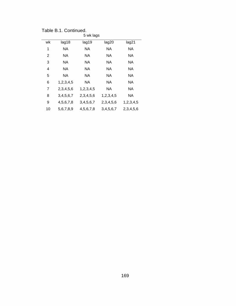
Table B.1. Continued. 5 wk lags
wk lag18 lag19 lag20 lag21
1 NA NA NA NA
2 NA NA NA NA
3 NA NA NA NA
4 NA NA NA NA
5 NA NA NA NA
6 1,2,3,4,5 NA NA NA
7 2,3,4,5,6 1,2,3,4,5 NA NA
8 3,4,5,6,7 2,3,4,5,6 1,2,3,4,5 NA
9 4,5,6,7,8 3,4,5,6,7 2,3,4,5,6 1,2,3,4,5
10 5,6,7,8,9 4,5,6,7,8 3,4,5,6,7 2,3,4,5,6
169

APPENDIX C
MANUFACTURER PROTOCOLS FOR
WEST NILE VIRUS SCREENING METHODS
170

Figure C.1. Manufacturer’s protocol for TRI-reagent®.
171
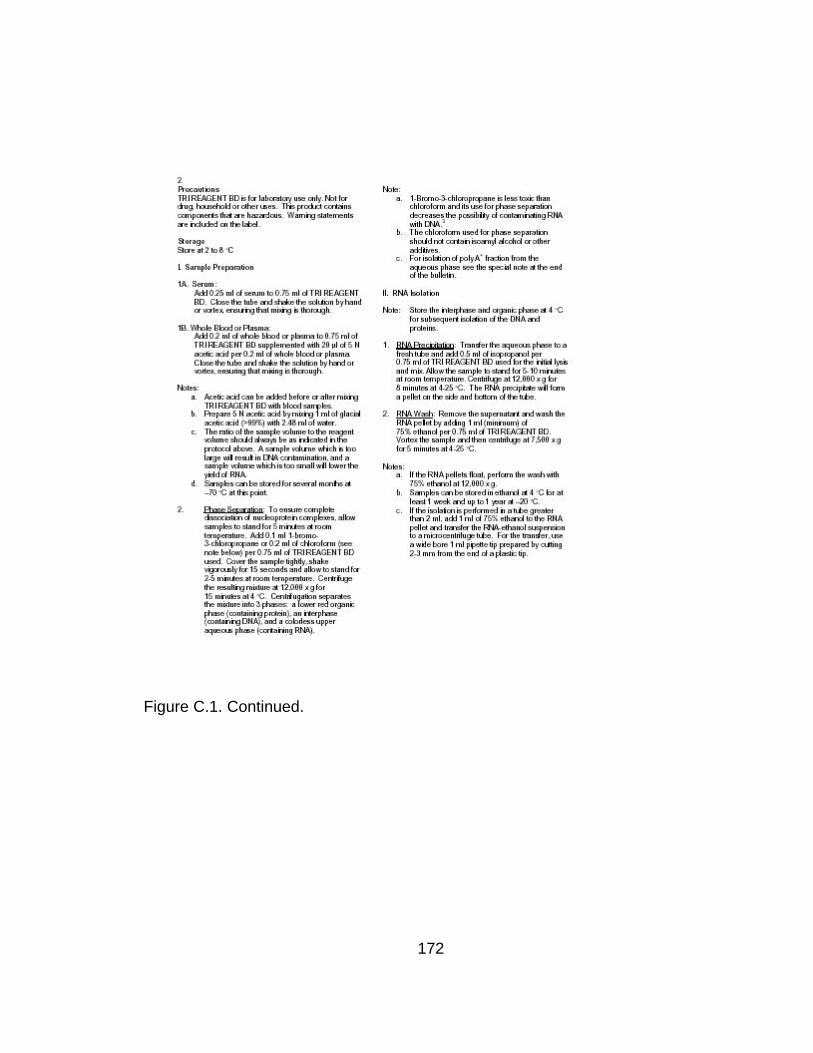
Figure C.1. Continued.
172

Figure C.1. Continued.
173

Figure C.1. Continued.
174

Figure C.1. Continued
175

Figure C.2. Manufacturer’s protocol for Access QuickTM RT-PCR System.
176
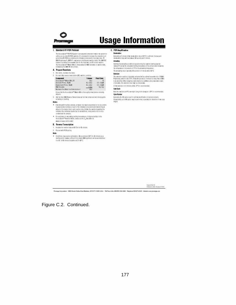
Figure C.2. Continued.
177

Figure C.3. Manufacturer’s protocol for the VecTest® Antigen Panel Assay.
178

Figure C.3. Continued.
179

Figure C.3. Continued.
180
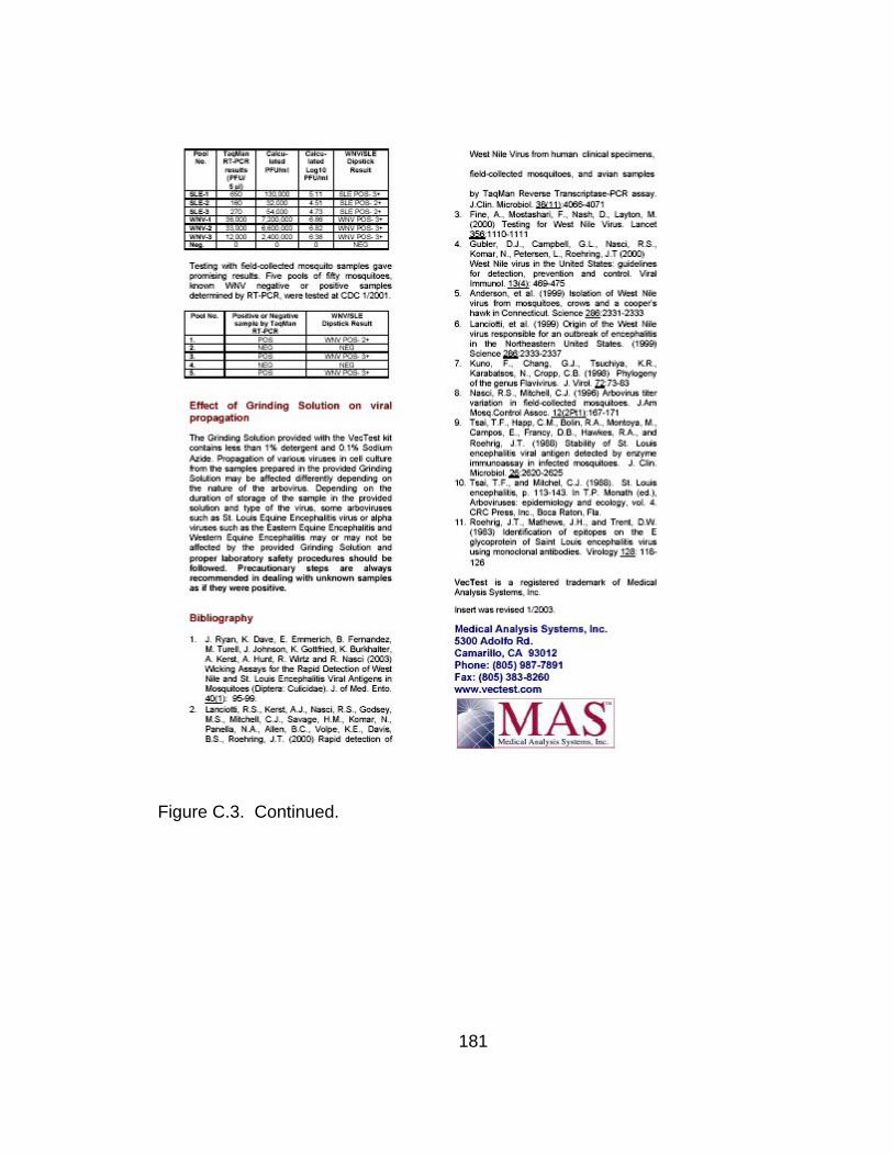
Figure C.3. Continued.
181