1

Effects of TV Contracts on NBA Salaries

Troy Kelly

Economics Honors

Spring 2017

Abstract:

This paper constructs a panel of player-season observations of performance statistics and salaries

for every player that has been in the National Basketball Association from 2002 to the start of the

2016-2017 season, with the exclusion of players that are on their rookie contract. I use player

and season fixed effects to help determine the overall effect of TV contracts and CBA deals on

players’ salaries in the NBA. This paper then utilizes a difference-in-difference-in-difference

model to draw out the distributional effects of these deals. The results of this paper suggests that

the new 2016 TV contract is the first time we see a positive impact on players’ salary in the

NBA, specifically players who are above the median salary in a given year, after 15 years of TV

deals and new league policies brought on by the CBA. However, this paper also concludes that

over the course of these 15 seasons, the wage inequality gap has been rising in the NBA between

low caliber “nonunionized” players and the high caliber “unionized” stars.

Keywords: Salaries, television contracts, NBA, union, star-power

JEL Codes: Z22,J31

Acknowledgements:

I would like to especially thank Professor Benjamin Anderson of the Colgate University

Economics Department for his help and advice throughout this research process. I would also

like to extend thanks to Professor Carolina Castilla of the Colgate University Economics

Department for her help and guidance during this process.

2

Introduction:

In labor economics, the idea of distribution of income, or wages, among unionized and

nonunionized workers is a topic that has been looked at for many years with differing results.

Freeman (1980) split the impact of unions on the distribution of wages into two effects. The

“within-sector” effect was the idea of wage inequality within the union itself, while the

“between-sector” effect was the idea of wage inequality between union and nonunion workers.

Freeman (1980) concluded that unions actually reduce wage inequality among men because the

“between-sector” effect was smaller than the “within-sector” effect. This means that the wage

inequality was decreasing within the union, but the inequality was increasing between the union

and nonunion workers. Card et al. (2004) took this study a step further and looked at 30 years of

data across the United States, United Kingdom, and Canada, and found the same results that

unions reduce the variance of wages. One difficult problem with studying labor economics is

how to correctly measure for productivity of the workers. My study will contribute to the

existing literature on unions and wage disparity by including accurate measures of productivity

through the on-court performance statistics of the players in the National Basketball Association.

The idea of unions in the National Basketball Association can be thought of in two ways.

The first way is that the only nonunionized players are the rookies and players on their rookie

contract since they see different rules and limits, and all of the rest of the players in the NBA are

in a union that is governed by the rules of the Collective Bargaining Agreement and the National

Basketball Players Association. The second way is that the star players are in a union since they

have higher bargaining power, while the rest of the league is considered to be nonunionized. I

will contribute to the preexisting literature by accurately measuring the effects and changes of

unionized and nonunionized workers with regards to wage disparity through controlling for the

3

TV contracts that increase the amount of revenue available to be bargained for and the CBA

deals that affect the distribution of revenue.

This paper will build upon previous studies that have looked at pay and performance in

the NBA.1 Since no previous study has looked at the effects of television contracts on salaries in

the NBA, MLB, NHL, and NFL, my contribution will be to build a model that includes TV

contracts and CBA deals to determine these effects on salaries. There has been uncertainty on

whether over time the increases in basketball related income is passed through to players in new

salaries by the amount it should. For instance, a new TV contract should impact the basketball

related income, but not the player benefits or shared percentage of revenue that goes to the

players. As such, the change in player salaries should be close to the change in salary cap

brought on by this increase in basketball related income.

This paper will then seek to answer the question of how the changes in revenue brought

on by the new television deals and collective bargaining agreements are distributed throughout

the league. The question is that do we see the majority of the money going to the superstars or is

the revenue used to build around the superstars and thus spread more to the role players. This

will allow me to incorporate the ideas of salary inequality between within and between unionized

and nonunionized players. I will do this by analyzing the change in salaries for players above

and below the median salary, and the 20th

and 80th

percentiles in the league and compare these

changes over the course of the CBA and TV deals.

1 For a review of the previous literature exploring the relationship between on-court productivity and salary, please

refer to Berri and Simmons (2011), Bodvarrson and Barstow (1998), Yang and Lin. (2012), and Lee et al. (2009).

Additionally, the literature has considered the effect of race (Dey, 1997; Gius and Johnson, 1998), “star-power”

(Dey, 1997; Hausman and Leonard, 1997; Berri and Schmidt, 2006), and nationality (Yang and Lin, 2012; Eschker

et al., 2004) upon salary. I draw upon the previous literature to determine the relevant on-court productivity

measures to include in this analysis and incorporate player fixed effects to control for unobservable, time invariant

player characteristics that might affect salary.

4

The literature review is broken down into two parts. The first part will discuss the history

and background of the NBA TV contracts and the collective bargaining agreements. Then the

second part will analyze studies done on the effects of on court performance and other factors

that determine a player’s salary. I will then discuss my data and the possible issues and

restrictions with this data. Afterwards, I will discuss the methodology and the first three models

of the study. Then I will present the results and draw out these results through a difference in

difference in difference model. Finally, I will discuss these results and run robustness checks to

clarify issues and conclude my paper.

Background:

Every few years, professional sports leagues choose to sign new lucrative television

contracts. In 2015, Americans spent 31 billion hours watching sports on their television, which

is a 40% upgrade from 2005 (James, 2017). Even though basic cable channels, including ESPN

and TNT, have lost more than 8 million subscribers since 2010 through the phenomenon known

as cord-cutting, sports programming as a whole generates $30 billion a year in revenue for

television companies (James, 2017). According to the audience measurement firm Nielsen, since

2005, broadcast and cable TV executives have increased their hours of sports programming by

160% (James, 2017).

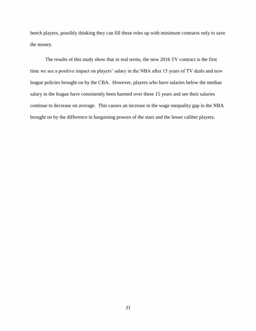
Since 2002, the National Basketball Association (NBA) has signed three separate

television contracts. After the most recent 2015-2016 NBA season, the newest NBA television

contract came into effect with TNT, ESPN, and ABC. This new television contract is worth $24

billion, compared to the previous television contract, which was implemented after the 2007-

2008 NBA season, and was worth $7.4 billion, or $8.6 billion in 2016 dollars.

5

The NBA has also signed four separate collective bargaining agreements since 1999. The

collective bargaining agreement, or CBA, is a “legal contract between the league and the players

association that sets up the rules by which the league operates” (Coon, 2016). The CBA

ultimately defines the salary cap and how it is set, the minimum and maximum salaries for

players, procedures for the NBA draft, and many more rules and topics that allow the NBA to

function as a whole and maintain its competitive balance (Coon, 2016). The signing of the most

recent television contract led to an increase in league revenue. This increase in revenue was then

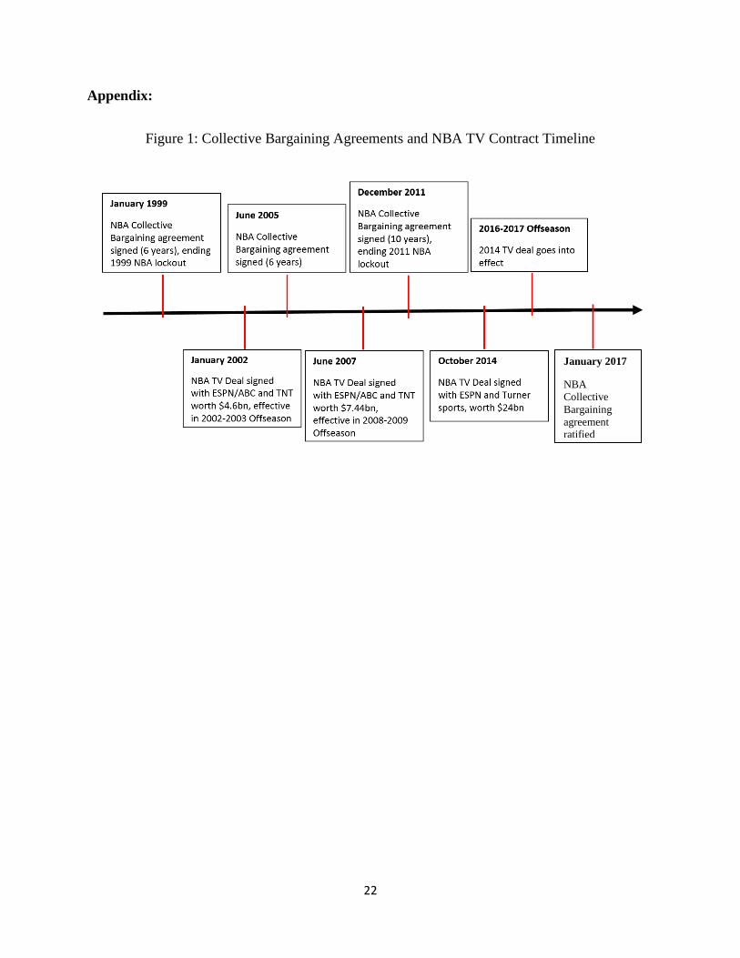
distributed equally throughout the league and thus, as shown in Graph 1, pushed the 2016-2017

team salary cap to $94,143,000, up from $70,000,000 and $63,065,000 in the 2015-2016 and

2014-2015 seasons respectively (Sports Reference, 2016).

As shown by Figure 1, the most recent collective bargaining agreements were signed in

1999, 2005, 2011, and January of 2017. The collective bargaining agreement, or CBA, is an

agreement between the National Basketball Association and the National Basketball Players’

Association (NBPA). This agreement includes legal and financial documents that controls

employment terms and conditions of NBA players and also includes all parts of NBA business

(Wong et al., 2010). The CBA is largely emplaced to maintain a competitive balance amongst

the league. Competitive balance in sports is the idea that no one team has an unfair advantage in

the league over another team. One of the most important ways the collective bargaining

agreement tries to maintain league wide competitive balance is through the issuance of a salary

cap. The NBA was the first professional sports league to issue a salary cap, which was

established in the 1984-1985 season at $3.6 million per team (Wong et al., 2016). Today, the

salary cap is at $94,143,000 per team, which is an increase of roughly 2500% since the original

6

salary cap in 1985. Currently, the NBA salary cap is determined by the following equation

(Wong et al., 2016):

(49 − 51%) 𝑃𝑟𝑜𝑗𝑒𝑐𝑡𝑒𝑑 𝐵𝑅𝐼 − 𝑃𝑟𝑜𝑗𝑒𝑐𝑡𝑒𝑑 𝐵𝑒𝑛𝑒𝑓𝑖𝑡𝑠 𝑓𝑜𝑟 𝑃𝑙𝑎𝑦𝑒𝑟𝑠

30 𝑇𝑒𝑎𝑚𝑠

The projected BRI is defined as “Basketball Related Income” which accounts for all revenues

received by the teams, the league and their related entities in predetermined percentages, which

include ticket sales, broadcasting fees, naming rights, interest income, in-stadium revenues,

luxury box sales, etc. (NBPA, 2011). The projected player benefits include medical treatment,

401K plans, and others. As shown through the above formula, the players receive 49-51% of the

projected BRI less projected benefits for players. According to the 2005 CBA deal, the NBA

players were guaranteed 57% of BRI (Wyman, 2011). This decrease in compensation to the

players came as a result from the turmoil throughout the league before the signing of the 2011

CBA. After the 2008 financial crisis, NBA teams and owners had aggregate losses totaling in

the hundreds of millions of dollars over the last few seasons leading up to the 2011 CBA deal

(Wyman, 2011). The owners demanded that they received an increased portion of BRI to

compensate for these losses, and as a result, the National Basketball Players’ Association and the

NBA could not compromise and sign a new CBA deal in time for the 2011 season, resulting in a

lockout for the season. This lockout lasted until December of 2011 when the new CBA deal was

ratified and resulted in the NBA season being shortened from 82 games to 66 games. The

owners saw a big win from these negotiations due to their increase in BRI distribution while the

players took a heavy loss. This change from 57% to 49-51% constituted a loss of $270 million

to the players, or $610,000 per player (Wyman, 2011).

7

The 2011 CBA deal also brought about other changes with regards to the teams’ salary

cap. Teams now had to spend a minimum of 85% of the salary cap in the first two years after the

2011 CBA deal and then 90% of the salary cap there on out, while the 2005 CBA deal stated that

the teams had to spend only a minimum of 75% of the salary cap (Wyman, 2011). This increase

in the salary cap floor would possibly result in an increase in salaries offered to players so that

their respective teams could hit the minimum that they were required to spend. With regards to

the salary cap ceiling, the NBA has a “soft salary cap.” A soft salary cap means that teams are

allowed to go over the cap for certain reasons. These reasons are mainly for teams to retain its

own players and make trades that may exceed the cap under certain conditions (Coon, 2016).

However, there is a punishment for teams that go over the cap in the form of a luxury tax. This

luxury tax is an incremental tax that increases with every $5 million above the salary cap ($1.50,

1.75, 2.50, 3.25, etc.), and then this tax paid is split evenly between the rest of the teams in the

league who are not currently paying a luxury tax. There is also now a harsher $1 additional

penalty ($2.50, 2.75, 3.50, 4.25, etc.) repeat offenders, or teams that have paid a luxury tax in

four of the last five seasons (Wyman, 2011). This luxury tax is largely in effect to maintain a

competitive balance in the league so that one team cannot pay all of their players’ maximum

contracts and thus have all of the best players. It allows smaller market teams to be able to

compete and offer contracts that large market teams do not have room for in their salary cap.

Data:

I construct a panel of player-season observations of performance statistics and salaries for

every player that has been in the National Basketball Association from 2002 to the start of the

2016-2017 season, with the exclusion of players that are on their rookie contract. The majority

of the salary data is retrieved from ESPN, while the remaining salaries are retrieved from

8

Basketball-Reference. The performance statistics and other player information used in the

models are also retrieved from Basketball-Reference. The dependent variable will be the log of

salaries measured at the individual level and the salaries will also be normalized to real 2016

U.S. dollars.

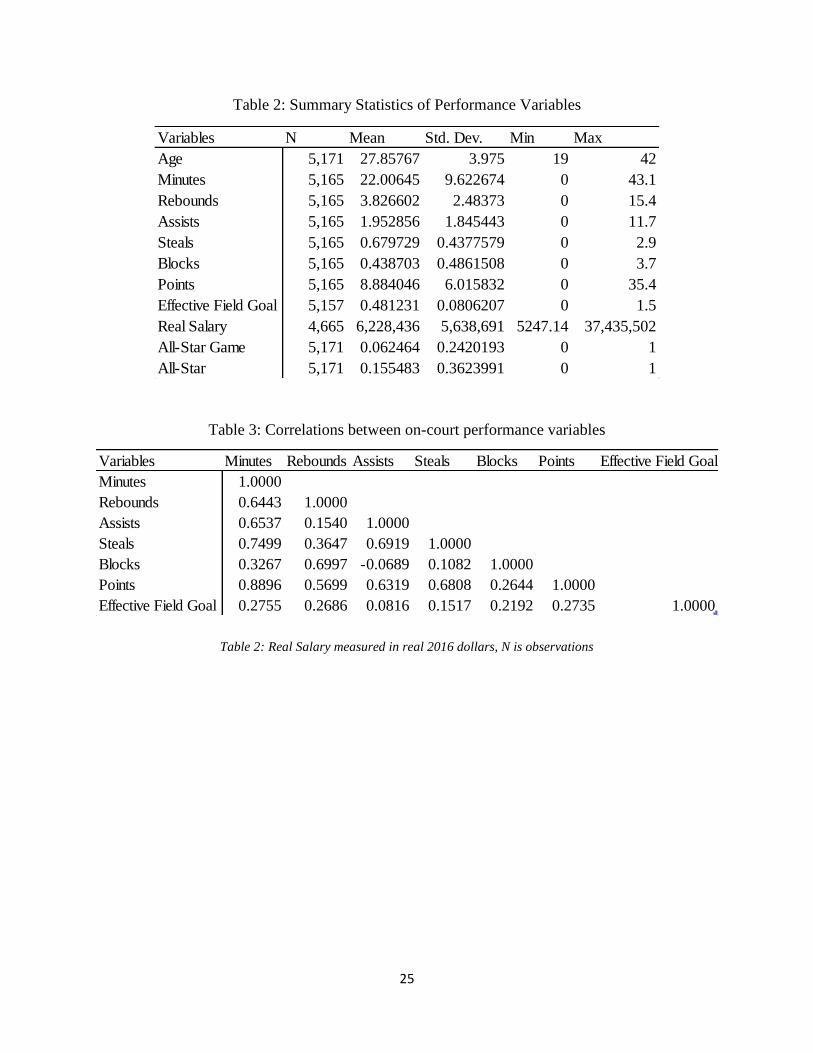
The performance variables, summarized in Table 2, are the most common measures of

on-court productivity that were used in previous studies by Berri and Simmons (2011),

Bodvarrson and Barstow (1998) and Yang and Lin (2012). These variables include: points

(PTS), assists (AST), total rebounds (TRB), steals (STL), blocks (BLK), and minutes (MPG). I

also included effective field goal percentage (eFG) as an advanced statistic of the overall

effectiveness of a player. Effective field goal percentage is measured as (Field Goals made + 0.5

x Three Point field goals made)/Field Goals attempted. These variables will all be measured at a

per game basis to control for any anomalies that may affect the results. If a player gets injured

and has to miss a large part of the season, their per game statistics would not be affected, but

their total statistics for that season would be skewed down. Also, total season statistics would be

skewed down league wide during the shortened 2011-2012 NBA season due to the NBA lockout,

but per game statistics would not be affected. Minutes per game was chosen rather than games

played or games started to control for injuries and players like Manu Ginobili, who plays the

majority of a game, but never starts.

One possible issue with using the on-court productivity values as independent variables is

that they are highly correlated with each other. As shown in Table 3, points per game and steals

per game have a correlation coefficient of 0.89 and 0.75 with minutes per game, respectively.

Other variables also have around a 0.70 correlation coefficient with each other which is

concerning. Lee, Leonard, and Jeon (2009) noted that one problem that may arise from this

9

multicollinearity is that the p-values of the individual regressors may be estimated too high or

even change the sign of the estimated coefficient. They then mention that one way to mitigate

this problem is to increase the number of observations. Since the study conducted by Lee,

Leonard, and Jeon (2009) had 2,262 salary observations while this study has 4,665 observations,

I believe multicollinearity concerns are decreased.

The All-Star Game appearance (ASG) variable will be a dummy variable that will be

equal to one if the player was elected to the All-Star Game for that particular season and zero if

otherwise. The other All-Star dummy variable (AG) is set to be equal to one once a player has

been named to the All-Star team once and equal to one for all future seasons, and zero for all

seasons prior to that year, or if the player has never been elected to the all-star game. With

regards to the age variable, both age and age squared will be included due to NBA players’ age

not having a linear relationship with their salaries since there is typically a diminishing marginal

return with a player’s age and productivity in professional sports.

The six models being analyzed will be run using player and year fixed effects. Player

fixed effects is utilized to control for time invariant factors that may affect a player’s salary, like

draft position and position. It will also control for the unobserved skills players have that would

typically not change over time, or are hard to measure, like athleticism, potential, basketball IQ,

and heart. Dey (1997) determined there was a significant effect of a player’s position on their

salary; however a player’s position typically does not change over the course of their career, so it

would be dropped from the player fixed effects model due to being time invariant. There has

also been speculation on whether discrimination based on race and nationality is apparent in the

NBA. Dey (1997) and Gius and Johnson (1998) both determined that race was no longer an

issue, while Eschker, Perez, and Siegler (2006) concluded that there is no longer a premium paid

10

to international players. These speculative variables will not be included in this model due

running player fixed effects and these variables being time invariant. Using year fixed effects,

along with player fixed effects, will help deal with unobservable variations that would affect all

of the players in the league. One main example would be the financial crisis.

This study will exclude any rookies until they sign their next contract after their rookie

contract has completed, which is typically after two years. Some players, however, remain on

their rookie contract for up to four years due to their respective team exercising a team option. A

team option is an option that allows the team to extend the player’s contract through one

additional season, and can be exercised two times for rookie contracts, making the player be on

their rookie contract for up to four years. I chose to not include players on their rookie contract

because this contract they sign upon being drafted is largely dependent on their draft position,

collegiate statistics, and unobservable skills, like athleticism and potential, and these measured

would be controlled for by using player fixed effects.

Graph 2 shows the summary statistics of the average NBA player’s salary in real 2016

dollars for each season analyzed in this study. The two seasons to highlight are the 2008-2009

season and the 2016-2017 season. These seasons are both immediately after a new TV contract

is implemented. As shown in Graph 2, the average salary in the 2008-2009 season is

$6,500,603, which is higher than any of the surrounding seasons. This increase in salary,

although small, may be correlated to the higher league revenues, and thus team salary caps,

brought on by the new TV contract. The average NBA salary in the 2016-2017 season is

$7,798,035, which is an increase of over $1,600,000 from the previous season. This larger

increase, compared to the smaller increase in the average salaries in the 2008-2009 season, could

11

be due to the fact that the newest TV contract was about three times as large as the previous TV

contract.

Methodology:

The first model analyzed will be used to determine the average effects of the TV

contracts on NBA salaries, controlling for performance variables, but without taking into account

the CBA deals.

lnSalaryit = β0 + β1Xit + 𝛿1TV2t + 𝛿2TV3t + αi + uit (1)

The Xit in this model includes all of the performance variables (PTSit + ASTit + TRBit + STLit +

BLKit + MPGit + Ageit + Age2it + eFGit + ASGit + AllStarit). The i refers to player i, while t is

season t. All of the performance variables, excluding age, age2, and All-Star, will be lagged by

one year. The reason for lagging the other on-court productivity variables is because typically a

player’s new contract is signed and negotiated based off of the player’s previous season

statistics. Also, many contracts are signed in the off-season, before the player has any statistics

for the current season.

The TV2 variable is a dummy variable that will equal one if the current contract year is

between 2008 and 2015 and zero if otherwise. The TV3 variable is a dummy variable that will

equal one if the current contract year observed is the 2016 season. The baseline for these dummy

variables is the first TV contract, from years 2002-2007 in this study. The coefficient on the

TV2 dummy will show the effect of the 2008 TV contract on the average NBA salary,

controlling for on-court productivity variables. The coefficient on the TV3 dummy will show

the effect of the 2016 TV on the average NBA salary, controlling for on-court productivity

12

variables. I expect to see both coefficients to be positive and significant, with a larger coefficient

for TV3 due to the larger revenue based contract.

The second model will be used to determine the average effects of the CBA deals on

NBA salaries, without taking into account the TV deals, and controlling for the performance

variables.

lnSalaryit = β0 + β1Xit + 𝛿3CBA2t + 𝛿4CBA3t + αi + uit (2)

The Xit in this model is the performance variables as mentioned from model (2). The CBA2

variable is a dummy variable that is equal to one if the current contract observed is in 2005

through the 2010 season and equal to zero if otherwise. The CBA3 variable is a dummy variable

that is equal to one if the current contract observed is from the 2011 season and later and equal to

zero if otherwise. The baseline for these dummy variables is the first CBA contract, or from the

years 2002-2005 of this study. Similar to Model (1), the coefficients on the respective CBA

dummy variables will show the effect of the corresponding CBA deal on the average NBA

salary. I expect to see the CBA2 variable to have either a very small significance, or no

significance due to there not being any prominent changes in this CBA deal with regards the

previous CBA. I expect the CBA3 variable to have a negative and significant coefficient due to

the previously mentioned change in the CBA that forced players to now receive 49-51% of the

league BRI rather than 57% in the previous CBA.

The third model that is analyzed will be used to determine the actual effect of the

individual CBA deals and TV contracts on players’ salaries. Since the CBA deals and TV

contracts change during each other, this model should control for these changes and the

coefficients should accurately represent the impact of the individual deals

13

lnSalaryit = β0 + β1Xit + 𝛿1TV2t + 𝛿2TV3t + 𝛿3CBA2t + 𝛿4CBA3t + 𝛿5Treatment1it +

𝛿6Treatment2it + 𝛿7Treatment3it + 𝛿8Treatment4it + 𝛿9- 𝛿23Seasont + αi + uit (3)

The Treatment1 variable is a dummy variable that is created to measure the actual impact

of the 2008 TV contract on a player’s salary. If a player in the NBA signed a contract extension

between the 2006 and 2015 seasons, this variable is equal to one. A contract extension means

the player signed a new contract before their current contract expires. This means that new

contract does not go into effect, or count towards the respective team’s salary cap, until the

following year. This variable is also equal to one if a player signed a new contract, besides a

contract extension, between the 2007 and 2016 seasons. If Treatment1 is equal to one, that

means that the player signed a contract or extension during the years of the study that were

affected by the 2008 TV contract and not the 2016 TV contract or the 2002 TV Contract. The

Treatment2 variable is a dummy variable that is created to measure the actual impact of the 2016

TV contract on a player’s salary. This variable is equal to one if a player in the NBA signed a

contract extension in the 2015 season, or if a player signed a new contract, not including contract

extension, in the 2016 season. These variables will compare the players who signed a new

contract under the specific TV contract with the players who did not.

The Treatment3 and Treatment4 variables are very similar to the previously mentioned

Treatment1 variable. For Treatment3, this variable is equal to one if a player signed a contract

extension between the 2003 and 2010 seasons. It is also equal to one if a player signed a new

contract, which was not an extension, between the 2004 and 2011 seasons. This variable is

created to measure the impact of the 2005 CBA deal on the new salary contracts that were signed

during the deal’s oversight. The Treatment4 variable is equal to one if a player signed a contract

extension in the 2010 season or after, or if a player signed a new contract that is not an extension

14

at any point after the 2010 season. These variables will compare the players who signed a new

contract under the corresponding CBA with the players who did not sign a new contract.

Results:

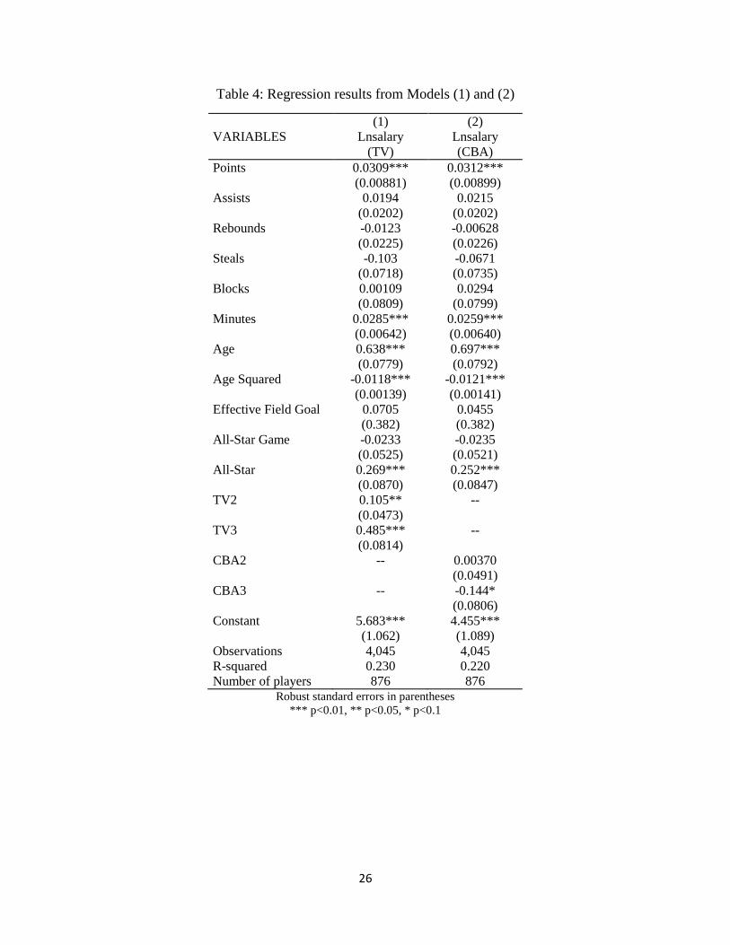
The results from models (1) and (2) are shown in Table 4. These models show the

average effect of the TV contracts and CBA deals separate from each other. The 2008 TV

contract increased the average NBA salary by 10.5%, while the 2016 TV contract increased the

average NBA salary by 48.5%. These two variables are significant at the 5% and 10%

respectively. This is consistent with my expectation because with the increase in league revenue

and thus team salary caps, teams would then have more money to spend and thus increase the

average salary paid to the players. The TV3 coefficient was also expected to be larger than the

TV2 coefficient due to the sheer magnitude of the increase in salary caps for the corresponding

years after each TV contract. With regards to the CBAs, the 2005 CBA had no effect on the

average NBA salary, which was expected. The 2011 CBA led to a decrease of 14.4% in average

NBA salaries, and is significant at the 10%. This is consistent with expectations since the

players were only guaranteed 49-51% of BRI, rather than the 57%.

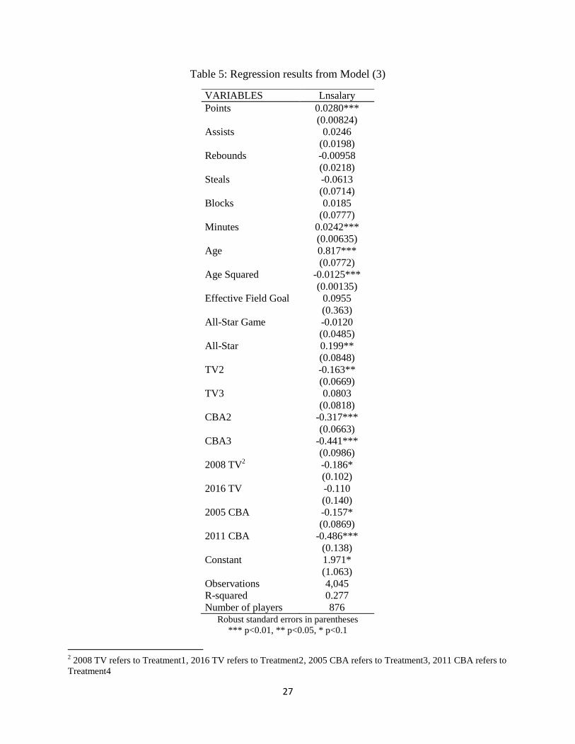
Table 5 shows the results from Model (3). Model (3) shows the effect of the TV

contracts combined with the CBA deals on NBA players’ average salaries. Relative to the

average NBA salary of players who did not sign a new contract, players who signed a new

contract while the 2005 CBA was in order saw their salaries decrease by 15.7%, significant at the

10% level, while players who signed a new contract while the 2011 CBA was in rule saw their

salaries decrease by an average of 48.6%, significant at the 1% level. Players who signed a new

contract under the 2008 TV contract had their salaries decrease by an average of 18.6%,

significant at the 10% level, while the effect of the 2016 TV contract on players signing a new

15

contract was insignificant. This model shows puzzling results with regards to the TV contracts

and players signing new contracts compared to players who do not sign a new contract. One

possible explanation for the results is distributional consequences. It is possible that the average

salaries of select groups of players are increasing, while other groups are decreasing, thus leading

to unexpected results when looking at the league as a whole.

To look at this possible distributional consequence in more depth, I had to run a

difference-in-difference-in-difference model. To do this, I will run model (3) three separate

times while including the new interactions to compare specific distributional groups within the

NBA.

lnSalaryit = β0 + β1Xit + 𝛿1TV2t + 𝛿2TV3t + 𝛿3CBA2t + 𝛿4CBA3t + 𝛿5Treatment1it +

𝛿6Treatment2it + 𝛿7Treatment3it + 𝛿8Treatment4it + 𝛿9TV2t*percentileit + 𝛿10TV3t*percentileit

+ 𝛿11CBA2t*percentileit + 𝛿12CBA3t*percentileit + 𝛿13Treatment1it*percentileit +

𝛿14Treatment2it*percentileit + 𝛿15Treatment3it*percentileit + 𝛿16Treatment4it*percentileit +

𝛿17percentileit + 𝛿18- 𝛿32Seasont + αi + uit (4) (5) (6)

In Models (4), (5), and (6), the variable labeled “percentile” will be replaced with the

corresponding salary boundary dummy variable of focus. The three salary boundaries of focus

in this study are the median, 20th

percentile, and 80th

percentile. The median dummy variable

will be equal to one if the player’s salary for the current year is above the median salary for the

NBA, and zero if it is below the median. The 20th

percentile dummy variable will be equal to

one if the player’s current salary is below the 20th

percentile salary for the NBA, and zero it is

above the 20th

percentile. The 80th

percentile dummy variable will be equal to one if the player’s

current salary is above the 80th

percentile salary for the NBA, and zero if it is below the 80th

percentile.

16

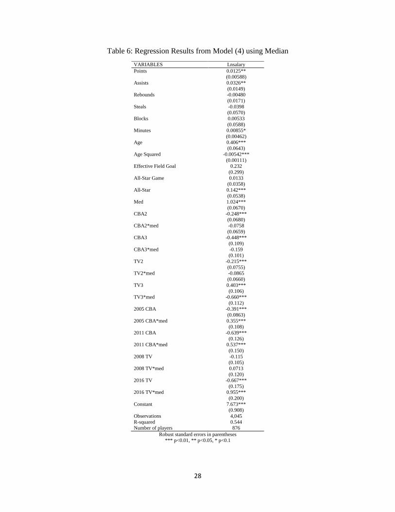
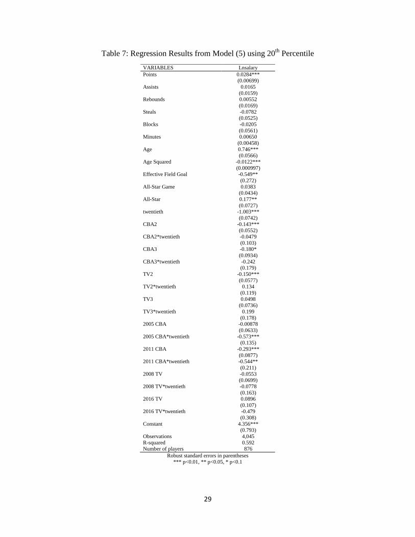
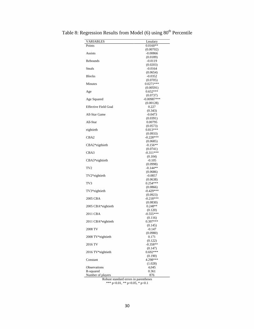
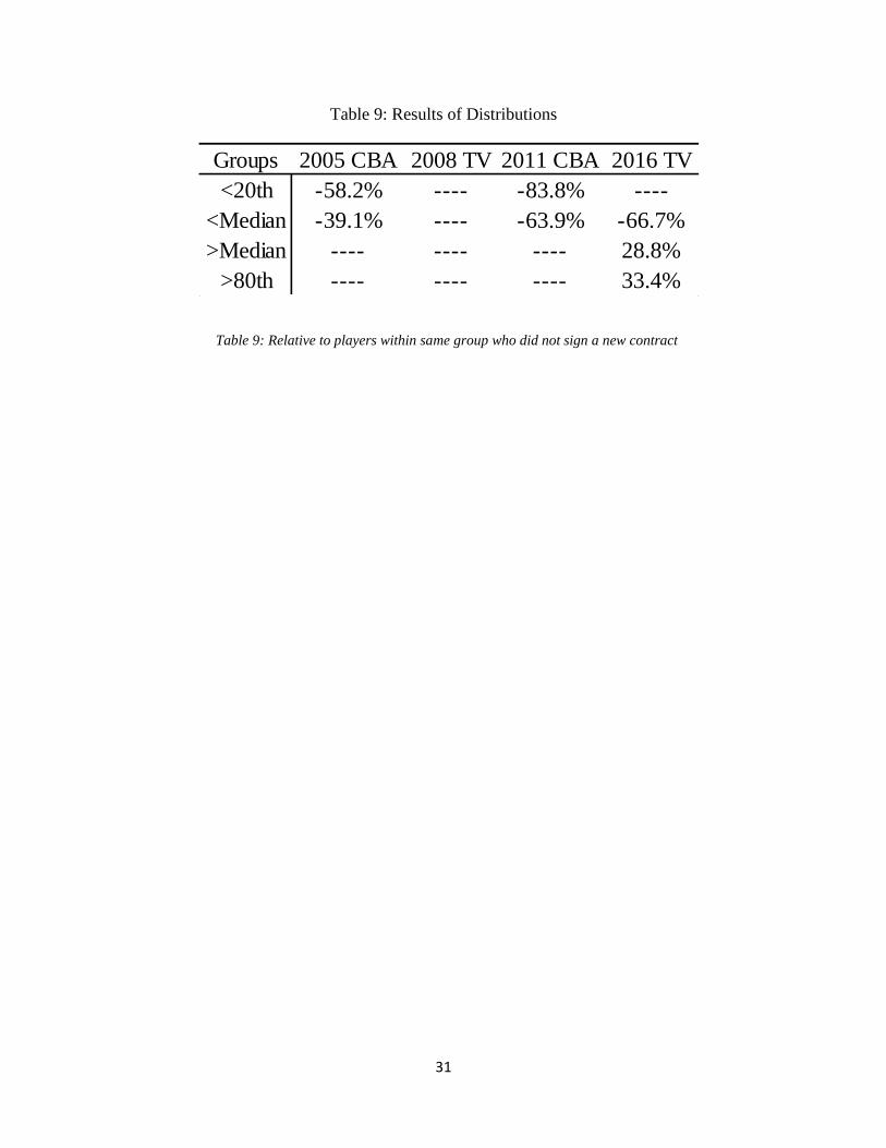
The results of Models (4), (5), and (6) are shown in Tables 6, 7, and 8 respectively.

Relative to the average salary of the players in the NBA below the median salary who did not

sign a new contract, players who did sign a new contract that was below the median during the

2005 CBA, after the 2011 CBA, or after the 2016 TV contract all saw a decrease in their salary

by 39.1%, 63.9%, and 66.7% respectively, while players who signed a new contract that was

below the median during the 2008 TV contract saw no change in their salaries. However,

relative to the average salary of players who were above the median that did not sign a new

contract, players who signed a new contract above the median during the 2005 CBA, 2008 TV

contract, or after the 2011 CBA saw no change in their salary, while players who signed a new

contract above the median after the 2016 TV contract saw an increase in their salary by 28.8%.

Looking at the combination of CBA deals and TV contracts in model (5), relative to the

average salary of players who were below the 20th

percentile who did not sign a new contract,

players who signed a new contract that was below the 20th

percentile salary during the 2005

CBA or after the 2011 CBA, saw their salaries decrease by 58.2% and 83.8% respectively, while

players who signed a new contract that was below the 20th

percentile salary during the 2008 TV

contract or after the 2016 TV contract saw no change in their salary.

Relative to the average salary of players who were above the 80th

percentile salary who

did not sign a new contract, players who signed a new contract that was above the 80th

percentile

salary in the NBA during the 2005 CBA, 2008 TV contract, or after the 2011 CBA contract, saw

no change in their salary. However, players who signed a new contract above the 80th

percentile

salary in the NBA after the 2016 TV contract saw an increase in their salary of 33.4%. All of

these results are summarized in Table 9.

17

These results help explain the puzzling results of Model (3). The 2016 TV contract was

insignificant with regards to players signing a contract compared to players who did not. This is

because the players who were above the median who signed a contract saw their salaries increase

relative to the players who did not sign a contract, while the players below the median who

signed a new contract saw their salaries decrease relative to the players who did not sign a

contract. These groups seem to cancel out the effects of each other, resulting in the 2016 TV

contract being insignificant to players signing a new contract.

With regards to the 2005 CBA and 2011 CBA in Model (3), players who signed a new

contract saw their salaries decrease relative to the average salaries of players who did not sign a

contract. This is consistent with the results from Models (4), (5), and (6) because for both deals,

the players below the median for who signed a new contract saw their salaries decrease relative

to the players below the median who did not sign a contract. Players above the median saw no

effect, so the decrease in salaries for players below the median dragged down the effect of the

deals as a whole. The larger negative impact of the 2011 CBA on all players who signed a

contract in Model (3) is also consistent with the results from Models (4), (5), and (6), with the

2011 CBA having a larger negative impact than the 2005 CBA.

Discussion:

With regards to labor economics and the idea of unionized and nonunionized players in

the NBA, wage inequality has been increasing over the past 15 years. If we consider all players

in the NBA, besides rookies, to be in a union, then the “within-sector” effect has been increasing.

We see players above the median salary who sign a new contract to either have no effect, or a

positive increase in their salaries after the 2016 TV contract. However, the players below the

median who sign a new contract are consistently harmed and see decreases in their salary. This

18

widens the wage inequality within the union. If we consider only the star players to be in a union

in the NBA due to their increased bargaining power, while the non-stars or role players to be

nonunionized, then the “between-sector” effect has been increasing. This is mainly due to the

bargaining power of the stars. When players of high caliber in the NBA are signing for large

contracts, the other similar high caliber players bargain to get similar deals, or else they will go

to another team, and since there is a limited supply of these high caliber players, teams are

willing to spend the maximum amount of money allowed. However, since there is a large supply

of low caliber players in the NBA, these players do not have the same bargaining power and are

typically looking to sign the minimum contracts so they can have a wage.

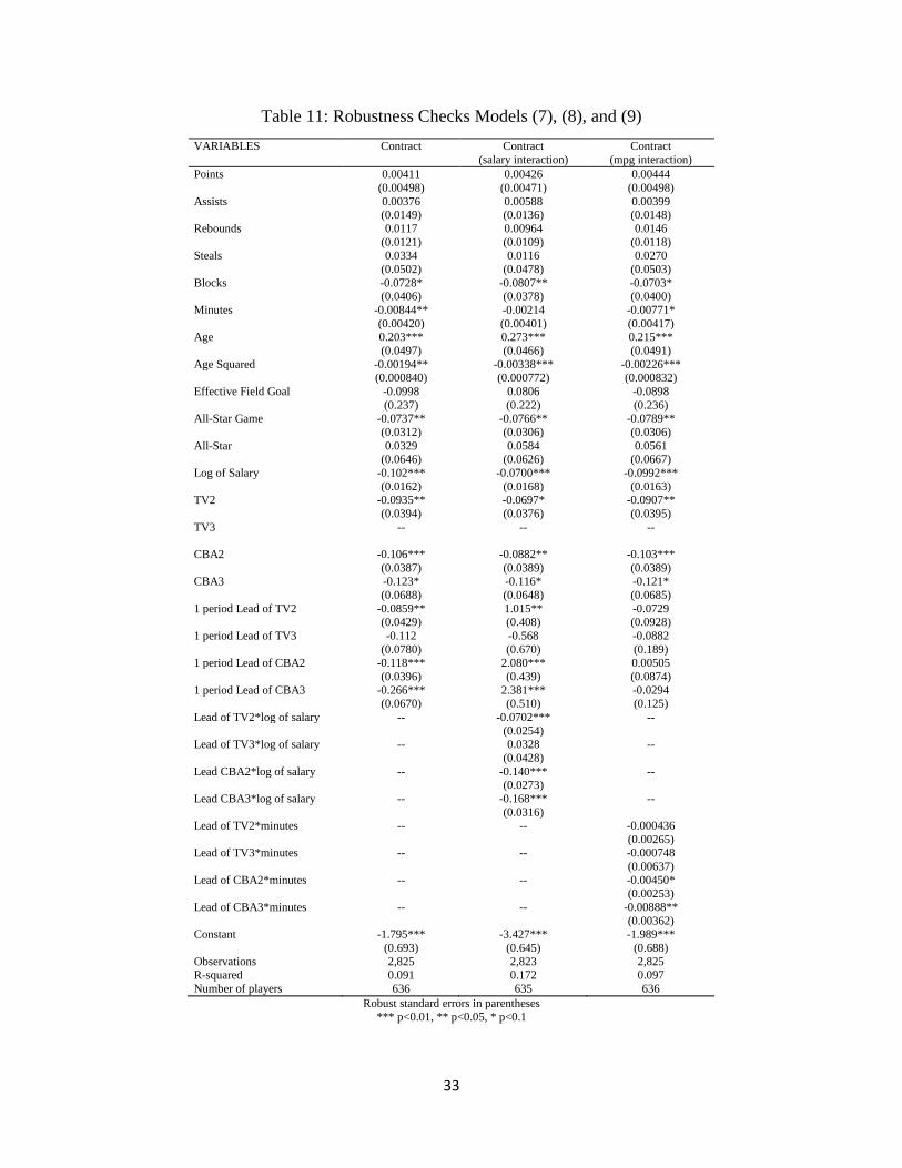
Robustness Checks:

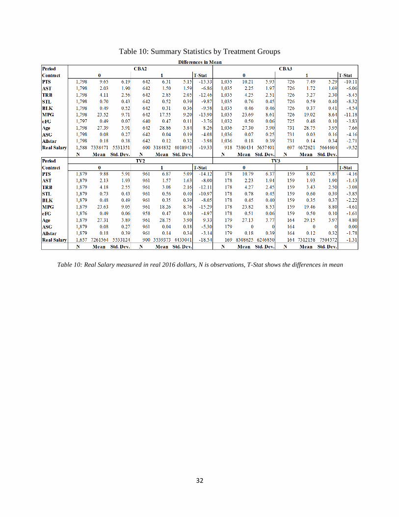
One possible concern with the results gathered from this study is the idea that players

may be strategically signing contracts to take advantage of these TV contracts and CBA deals.

The players that would be signing strategically to take advantage of these deals would be the

players with bargaining power, due to them theoretically being able to decide how long they sign

a contract for. However, upon further speculation, Table 10 shows that there are indeed

differences in the players that are signing contracts during these periods, but the majority of

players that sign contracts during these deals are the players of lesser caliber, rather than the high

caliber players. That is because the lesser caliber players are signing very frequently, sometimes

once or up to three times a year, while the high caliber players sign multi-year deals, typically

ranging from 2-4 years.

My next thought was that the high caliber players may be opting out of their contracts

and signing a new one just before the implementation of a new TV contract or CBA deal so they

can then sign again towards the beginning of the deal. I then ran a few robustness check models

19

and determined from the results in Table 11 that the players signing new contracts just before the

implementation of new deals have lower salaries and lower minutes per game. This suggests that

the lesser caliber players are still the ones signing the majority of the contracts just before a new

deal begins.

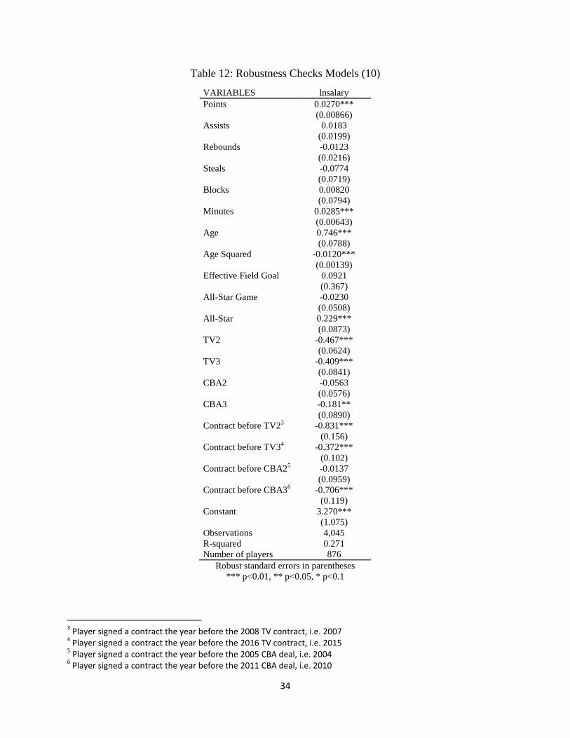
Finally, I ran another robustness check to see if the players signing just before the new

deals are taking advantage of these deals. The results in Table 12 show that the players who

signed a new contract just before the new TV contracts and CBA deals were not taking

advantage of these deals and signed for less. This suggests that they do not have the bargaining

power to sign for high contracts for one year in order to strategically sign again once the new

deal is implemented, and thus suggests again that the players signing before the new deals are

still the low caliber players.

These results make logical sense because in the NBA and other professional sports,

players have a larger uncertainty about their future than other areas of employment. For

example, these players may become injured, or not have the same statistics as they do currently.

Due to these reasons, most players will sign contracts for the largest amount of money and

longest periods of time as they can when they are able to and offered, rather than strategically

signing contracts to take advantage of changes in NBA policies or revenues.

Conclusions:

After the 2016 TV contract, there is a positive impact on players’ salaries that are above

the median salary in the league. The reasoning behind this could be due to the large increase in

league revenue, and thus team salary cap, all of the managers and coaches decide to put a stress

on signing superstars to form the idea of “superteams”. If the team cannot sign a superstar they

20

result in acquiring the next best talent, or starters or role players, to build around their current

stars. We see these two groups of players’ salaries increase in this period due to the rise in

competition between teams to sign these groups. One other thing to note is that the results of the

2016 TV contract only have one year of data, which could lead to altering results from the rest of

the periods due to having less observations.

Another thing to note is the results 2008 TV contract. This shows that there was no

impact on NBA player salaries from this TV contract. These results are interesting to note due to

the period in which this TV contract was enacted. While the 2008 TV contract was under the

rule of the 2005 CBA, and before the 2011 CBA contract, the financial crisis was a major part in

financial decision both in the finance world and professional sports. Owners across the league

may not have been willing to invest more money in their teams, or pay the necessary luxury tax

to sign certain players they needed. The year fixed effects may not have fully controlled for

these matters and that is why we see an opposing effect from the 2016 TV contract. The other

reason for a possible opposing effect is when the financial crisis was finally over, the 2011 CBA

began, which lowered the BRI that was guaranteed to all of the players, from 57% to 49-51%.

So this means the only observations we have for the 2008 TV contract are during the financial

crisis and the decrease in team salary cap.

One final interesting result to note is the results from the 2011 CBA itself. When the

owners voted to decrease the BRI that was guaranteed to players, the managers and coaches

decided where to take this money from. The results show that the players above the median

salary had saw no effect from this change in ruling, while the players below the median salary,

especially the players below the 20th

percentile salary, suffered. The managers and coaches

decided to keep the stars and starters happy by keeping their salaries the same, and harm the

21

bench players, possibly thinking they can fill these roles up with minimum contracts only to save

the money.

The results of this study show that in real terms, the new 2016 TV contract is the first

time we see a positive impact on players’ salary in the NBA after 15 years of TV deals and new

league policies brought on by the CBA. However, players who have salaries below the median

salary in the league have consistently been harmed over these 15 years and see their salaries

continue to decrease on average. This causes an increase in the wage inequality gap in the NBA

brought on by the difference in bargaining powers of the stars and the lesser caliber players.

22

Appendix:

Figure 1: Collective Bargaining Agreements and NBA TV Contract Timeline

January 2017

NBA

Collective

Bargaining

agreement ratified

23

Graph 1: Measured in real 2016 U.S. dollars, bars highlighted red are implementations of a TV contract of CBA

deal

$0.00

$10,000,000.00

$20,000,000.00

$30,000,000.00

$40,000,000.00

$50,000,000.00

$60,000,000.00

$70,000,000.00

$80,000,000.00

$90,000,000.00

$100,000,000.00

History of the Salary Cap (2016 Dollars)

Graph 1: History of the NBA Salary Cap

24

$-

$1,000,000

$2,000,000

$3,000,000

$4,000,000

$5,000,000

$6,000,000

$7,000,000

$8,000,000

$9,000,000

Mean of player salaries by year

Graph 2: Mean of Player Salaries by season

Graph 2: In real 2016 dollars, bars highlighted red are implementations of a TV contract of CBA deal

25

Table 2: Summary Statistics of Performance Variables

Table 3: Correlations between on-court performance variables

Variables N Mean Std. Dev. Min Max

Age 5,171 27.85767 3.975 19 42

Minutes 5,165 22.00645 9.622674 0 43.1

Rebounds 5,165 3.826602 2.48373 0 15.4

Assists 5,165 1.952856 1.845443 0 11.7

Steals 5,165 0.679729 0.4377579 0 2.9

Blocks 5,165 0.438703 0.4861508 0 3.7

Points 5,165 8.884046 6.015832 0 35.4

Effective Field Goal 5,157 0.481231 0.0806207 0 1.5

Real Salary 4,665 6,228,436 5,638,691 5247.14 37,435,502

All-Star Game 5,171 0.062464 0.2420193 0 1

All-Star 5,171 0.155483 0.3623991 0 1

Variables Minutes Rebounds Assists Steals Blocks Points Effective Field Goal

Minutes 1.0000

Rebounds 0.6443 1.0000

Assists 0.6537 0.1540 1.0000

Steals 0.7499 0.3647 0.6919 1.0000

Blocks 0.3267 0.6997 -0.0689 0.1082 1.0000

Points 0.8896 0.5699 0.6319 0.6808 0.2644 1.0000

Effective Field Goal 0.2755 0.2686 0.0816 0.1517 0.2192 0.2735 1.0000

Table 2: Real Salary measured in real 2016 dollars, N is observations

26

Table 4: Regression results from Models (1) and (2)

(1) (2)

VARIABLES Lnsalary

(TV)

Lnsalary

(CBA)

Points 0.0309*** 0.0312***

(0.00881) (0.00899)

Assists 0.0194 0.0215

(0.0202) (0.0202)

Rebounds -0.0123 -0.00628

(0.0225) (0.0226)

Steals -0.103 -0.0671

(0.0718) (0.0735)

Blocks 0.00109 0.0294

(0.0809) (0.0799)

Minutes 0.0285*** 0.0259***

(0.00642) (0.00640)

Age 0.638*** 0.697***

(0.0779) (0.0792)

Age Squared -0.0118*** -0.0121***

(0.00139) (0.00141)

Effective Field Goal 0.0705 0.0455

(0.382) (0.382)

All-Star Game -0.0233 -0.0235

(0.0525) (0.0521)

All-Star 0.269*** 0.252***

(0.0870) (0.0847)

TV2 0.105** --

(0.0473)

TV3 0.485*** --

(0.0814)

CBA2 -- 0.00370

(0.0491)

CBA3 -- -0.144*

(0.0806)

Constant 5.683*** 4.455***

(1.062) (1.089)

Observations 4,045 4,045

R-squared 0.230 0.220

Number of players 876 876 Robust standard errors in parentheses

*** p<0.01, ** p<0.05, * p<0.1

27

Table 5: Regression results from Model (3)

VARIABLES Lnsalary

Points 0.0280***

(0.00824)

Assists 0.0246

(0.0198)

Rebounds -0.00958

(0.0218)

Steals -0.0613

(0.0714)

Blocks 0.0185

(0.0777)

Minutes 0.0242***

(0.00635)

Age 0.817***

(0.0772)

Age Squared -0.0125***

(0.00135)

Effective Field Goal 0.0955

(0.363)

All-Star Game -0.0120

(0.0485)

All-Star 0.199**

(0.0848)

TV2 -0.163**

(0.0669)

TV3 0.0803

(0.0818)

CBA2 -0.317***

(0.0663)

CBA3 -0.441***

(0.0986)

2008 TV2 -0.186*

(0.102)

2016 TV -0.110

(0.140)

2005 CBA -0.157*

(0.0869)

2011 CBA -0.486***

(0.138)

Constant 1.971*

(1.063)

Observations 4,045

R-squared 0.277

Number of players 876 Robust standard errors in parentheses

*** p<0.01, ** p<0.05, * p<0.1

2 2008 TV refers to Treatment1, 2016 TV refers to Treatment2, 2005 CBA refers to Treatment3, 2011 CBA refers to

Treatment4

28

Table 6: Regression Results from Model (4) using Median

VARIABLES Lnsalary

Points 0.0125** (0.00588)

Assists 0.0326**

(0.0149) Rebounds -0.00480

(0.0171)

Steals -0.0398 (0.0570)

Blocks 0.00533

(0.0588) Minutes 0.00855*

(0.00462)

Age 0.406*** (0.0643)

Age Squared -0.00542***

(0.00111)

Effective Field Goal 0.232

(0.299)

All-Star Game 0.0133 (0.0358)

All-Star 0.142***

(0.0538) Med 1.024***

(0.0670)

CBA2 -0.248*** (0.0680)

CBA2*med -0.0758

(0.0659) CBA3 -0.448***

(0.109)

CBA3*med -0.159 (0.101)

TV2 -0.215***

(0.0755) TV2*med -0.0865

(0.0660)

TV3 0.403*** (0.106)

TV3*med -0.660***

(0.112) 2005 CBA -0.391***

(0.0863)

2005 CBA*med 0.355*** (0.108)

2011 CBA -0.639***

(0.126) 2011 CBA*med 0.537***

(0.150)

2008 TV -0.115 (0.105)

2008 TV*med 0.0713

(0.120) 2016 TV -0.667***

(0.175)

2016 TV*med 0.955***

(0.200)

Constant 7.673*** (0.908)

Observations 4,045

R-squared 0.544 Number of players 876

Robust standard errors in parentheses

*** p<0.01, ** p<0.05, * p<0.1

29

Table 7: Regression Results from Model (5) using 20th

Percentile

VARIABLES Lnsalary

Points 0.0284*** (0.00699)

Assists 0.0165

(0.0159) Rebounds 0.00552

(0.0169)

Steals -0.0782 (0.0525)

Blocks -0.0205

(0.0561) Minutes 0.00650

(0.00458)

Age 0.746*** (0.0566)

Age Squared -0.0122***

(0.000997)

Effective Field Goal -0.549**

(0.272)

All-Star Game 0.0383 (0.0434)

All-Star 0.177**

(0.0727) twentieth -1.003***

(0.0742)

CBA2 -0.143*** (0.0552)

CBA2*twentieth -0.0479

(0.103) CBA3 -0.180*

(0.0934)

CBA3*twentieth -0.242 (0.179)

TV2 -0.150***

(0.0577) TV2*twentieth 0.134

(0.119)

TV3 0.0498 (0.0736)

TV3*twentieth 0.199

(0.178) 2005 CBA -0.00878

(0.0633)

2005 CBA*twentieth -0.573*** (0.135)

2011 CBA -0.293***

(0.0877) 2011 CBA*twentieth -0.544**

(0.211)

2008 TV -0.0553 (0.0699)

2008 TV*twentieth -0.0778

(0.163) 2016 TV 0.0896

(0.107)

2016 TV*twentieth -0.479

(0.308)

Constant 4.356*** (0.793)

Observations 4,045

R-squared 0.592 Number of players 876

Robust standard errors in parentheses

*** p<0.01, ** p<0.05, * p<0.1

30

Table 8: Regression Results from Model (6) using 80th

Percentile

VARIABLES Lnsalary

Points 0.0160** (0.00702)

Assists -0.00866

(0.0189) Rebounds -0.0119

(0.0203)

Steals -0.0164 (0.0654)

Blocks -0.0352

(0.0705) Minutes 0.0271***

(0.00591)

Age 0.652*** (0.0737)

Age Squared -0.00987***

(0.00128)

Effective Field Goal 0.227

(0.343)

All-Star Game -0.0473 (0.0391)

All-Star 0.00795

(0.0573) eightieth 0.813***

(0.0933)

CBA2 -0.228*** (0.0685)

CBA2*eigthieth -0.156**

(0.0741) CBA3 -0.311***

(0.104)

CBA3*eightieth -0.105 (0.0998)

TV2 -0.144**

(0.0686) TV2*eightieth -0.0857

(0.0638)

TV3 0.254*** (0.0866)

TV3*eightieth -0.429***

(0.0923) 2005 CBA -0.218***

(0.0830)

2005 CBA*eightieth 0.248** (0.120)

2011 CBA -0.555***

(0.116) 2011 CBA*eightieth 0.397***

(0.145)

2008 TV -0.147 (0.0980)

2008 TV*eightieth 0.171

(0.122) 2016 TV -0.358**

(0.147)

2016 TV*eightieth 0.692***

(0.190)

Constant 4.298*** (1.028)

Observations 4,045

R-squared 0.361 Number of players 876

Robust standard errors in parentheses

*** p<0.01, ** p<0.05, * p<0.1

31

Groups 2005 CBA 2008 TV 2011 CBA 2016 TV

<20th -58.2% ---- -83.8% ----

<Median -39.1% ---- -63.9% -66.7%

>Median ---- ---- ---- 28.8%

>80th ---- ---- ---- 33.4%

Table 9: Results of Distributions

Table 9: Relative to players within same group who did not sign a new contract

32

Table 10: Summary Statistics by Treatment Groups

Table 10: Real Salary measured in real 2016 dollars, N is observations, T-Stat shows the differences in mean

33

Table 11: Robustness Checks Models (7), (8), and (9)

VARIABLES Contract Contract Contract

(salary interaction) (mpg interaction)

Points 0.00411 0.00426 0.00444

(0.00498) (0.00471) (0.00498)

Assists 0.00376 0.00588 0.00399 (0.0149) (0.0136) (0.0148)

Rebounds 0.0117 0.00964 0.0146

(0.0121) (0.0109) (0.0118) Steals 0.0334 0.0116 0.0270

(0.0502) (0.0478) (0.0503)

Blocks -0.0728* -0.0807** -0.0703* (0.0406) (0.0378) (0.0400)

Minutes -0.00844** -0.00214 -0.00771*

(0.00420) (0.00401) (0.00417) Age 0.203*** 0.273*** 0.215***

(0.0497) (0.0466) (0.0491)

Age Squared -0.00194** -0.00338*** -0.00226*** (0.000840) (0.000772) (0.000832)

Effective Field Goal -0.0998 0.0806 -0.0898

(0.237) (0.222) (0.236) All-Star Game -0.0737** -0.0766** -0.0789**

(0.0312) (0.0306) (0.0306)

All-Star 0.0329 0.0584 0.0561 (0.0646) (0.0626) (0.0667)

Log of Salary -0.102*** -0.0700*** -0.0992***

(0.0162) (0.0168) (0.0163) TV2 -0.0935** -0.0697* -0.0907**

(0.0394) (0.0376) (0.0395)

TV3 -- -- --

CBA2 -0.106*** -0.0882** -0.103***

(0.0387) (0.0389) (0.0389) CBA3 -0.123* -0.116* -0.121*

(0.0688) (0.0648) (0.0685)

1 period Lead of TV2 -0.0859** 1.015** -0.0729 (0.0429) (0.408) (0.0928)

1 period Lead of TV3 -0.112 -0.568 -0.0882

(0.0780) (0.670) (0.189) 1 period Lead of CBA2 -0.118*** 2.080*** 0.00505

(0.0396) (0.439) (0.0874)

1 period Lead of CBA3 -0.266*** 2.381*** -0.0294 (0.0670) (0.510) (0.125)

Lead of TV2*log of salary -- -0.0702*** --

(0.0254) Lead of TV3*log of salary -- 0.0328 --

(0.0428)

Lead CBA2*log of salary -- -0.140*** -- (0.0273)

Lead CBA3*log of salary -- -0.168*** --

(0.0316) Lead of TV2*minutes -- -- -0.000436

(0.00265) Lead of TV3*minutes -- -- -0.000748

(0.00637)

Lead of CBA2*minutes -- -- -0.00450*

(0.00253)

Lead of CBA3*minutes -- -- -0.00888**

(0.00362) Constant -1.795*** -3.427*** -1.989***

(0.693) (0.645) (0.688)

Observations 2,825 2,823 2,825 R-squared 0.091 0.172 0.097

Number of players 636 635 636

Robust standard errors in parentheses

*** p<0.01, ** p<0.05, * p<0.1

34

Table 12: Robustness Checks Models (10)

VARIABLES lnsalary

Points 0.0270***

(0.00866)

Assists 0.0183

(0.0199)

Rebounds -0.0123

(0.0216)

Steals -0.0774

(0.0719)

Blocks 0.00820

(0.0794)

Minutes 0.0285***

(0.00643)

Age 0.746***

(0.0788)

Age Squared -0.0120***

(0.00139)

Effective Field Goal 0.0921

(0.367)

All-Star Game -0.0230

(0.0508)

All-Star 0.229***

(0.0873)

TV2 -0.467***

(0.0624)

TV3 -0.409***

(0.0841)

CBA2 -0.0563

(0.0576)

CBA3 -0.181**

(0.0890)

Contract before TV23 -0.831***

(0.156)

Contract before TV34 -0.372***

(0.102)

Contract before CBA25 -0.0137

(0.0959)

Contract before CBA36 -0.706***

(0.119)

Constant 3.270***

(1.075)

Observations 4,045

R-squared 0.271

Number of players 876

Robust standard errors in parentheses

*** p<0.01, ** p<0.05, * p<0.1

3 Player signed a contract the year before the 2008 TV contract, i.e. 2007

4 Player signed a contract the year before the 2016 TV contract, i.e. 2015

5 Player signed a contract the year before the 2005 CBA deal, i.e. 2004

6 Player signed a contract the year before the 2011 CBA deal, i.e. 2010

35

References:

Adams, Luke. “2013 NBA Rookie Scale Extensions.” HoopsRumor. (11/2013). Web. 4 May

2017.

Berri, David J., and Martin B. Schmidt. "On the Road With the National Basketball Association's

Superstar Externality." Journal of Sports Economics 7.4 (2006): 347-58. Web. 3

Dec. 2016.

Bodvarrson, Orn B., and Raymond T. Brastow. “Do employers pay for consistent performance?:

Evidence from the NBA.” Economic Inquiry 36.1 (1998): 145-60. 4 May 2017.

Card, David, Thomas Lemieux, and W. C. Riddell. “Unions and Wage Inequality.” Journal of

Labor Research 25.4 (2004): 519-59. ProQuest. Web. 4 May 2017.

Coon, Larry. “Larry Coon’s NBA Salary Cap FAQ.” (7/2016). Web. 28 Nov. 2016.

Dey, Matthew S. "Racial Differences in National Basketball Association Players' Salaries: A

New Look." The American Economist 41.2 (1997): 84-90. JSTOR. Web. 13 Oct. 2016.

Eschker, Erick, Stephen J. Perez, and Mark V. Siegler. "The NBA and the influx of international

basketball players." Applied Economics 36.10 (2004): 1009-20. Taylor Francis Online.

Web. 13 Oct. 2016.

Freeman, Richard B. “Unionism and the Dispersion of Wages.” Industrial and Labor Relations

Review 34 (10/1980): 3-23. Web. 4 May 2017.

36

Gius, Mark, and Donn Johnson. "An Empirical Investigation of Wage Discrimination in

Professional Basketball." Applied Economics Letters 5.11 (1998): 703-05. Taylor Francis

Online. Web. 13 Oct. 2016.

Hausman, Jerry A., and Gregory K. Leonard. "Superstars in the National Basketball Association:

Economic value and policy." Journal of Labor Economics 15.4 (1997): 586-624.

Web. 3 Dec. 2016.

James, Meg. “The rise of sports TV costs and why your cable bill keeps going up.” Los Angeles

Times. Accessed March 05, 2017.

Lee, Sang H., et al. “Sports market capacity, frequency of movements, and age in the NBA

players salary determination.” Indian Journal of Economics and Business 8.1,

(2009): 127+. Academic OneFile. 9 April 2017.

NBPA Collective Bargaining Agreement. “Basketball Related Income, Salary Cap, Minimum

Team Salary, and Escrow Arrangement.” Article VII. (2011). Page 86-204. Web. 3 Dec.

2016.

Scully, Gerald W. “Pay and Performance in Major League Baseball.” The American Economic

Review 64.6 (1974): 915–30. JSTOR. 9 April 2017.

Simmons, Rob, and David J. Berri. “Mixing the princes and the paupers: Pay and performance in

the National Basketball Association.” Labour Economics 18.3 (2011): 381-88. 4 May

37

2017.

Sports Reference LLC “NBA Salary Cap History.” Basketball-Reference.com – Basketball

Statistics and History. Web. 28 Nov. 2016. http://www.basketball-reference.com/.

Stanek, Tyler, "Player Performance and Team Revenues: NBA Player Salary Analysis.” (2016).

CMC Senior Theses. Paper 1257. Web. 15 Nov. 2016.

“Transactions.” NBA.com. (7/2010). Web. 4 May 2017.

Wyman, Alexander C.K., “Collective Bargaining and the Best Interests of Basketball.” (2012).

12 Va. Sports & Ent. L.J. 171 (2012). Web. 15 Nov. 2016.

Wong, Glenn M., and Chris Deubert. “National Basketball Association General Managers: An

Analysis of the Responsibilities, Qualifications and Characteristics” (December 4, 2010).

Villanova Sports and Entertainment Law Journal, Vol. 18, 2011. Web. 15 Nov. 2016.

Yang, Chih-Hai, and Hsuan-Yu Lin. “Is There Salary Discrimination by Nationality in the

NBA?: Foreign Talent or Foreign Market” Journal of Sports Economics 13.1 (2012): 53-

75. 4 May 2017.