EFFECTS OF STRAIN RATE VARIATION ON THE SHEAR …
100
The Pennsylvania State University The Graduate School Department of Aerospace Engineering EFFECTS OF STRAIN RATE VARIATION ON THE SHEAR ADHESION STRENGTH OF IMPACT ICE A Thesis in Aerospace Engineering by Rebekah Douglass © 2019 Rebekah Douglass Submitted in Partial Fulfillment of the Requirements for the Degree of Master of Science May 2019
Transcript of EFFECTS OF STRAIN RATE VARIATION ON THE SHEAR …

The Pennsylvania State University
The Graduate School
Department of Aerospace Engineering
EFFECTS OF STRAIN RATE VARIATION ON
THE SHEAR ADHESION STRENGTH OF IMPACT ICE
A Thesis in
Aerospace Engineering
by
Rebekah Douglass
© 2019 Rebekah Douglass
Submitted in Partial Fulfillment
of the Requirements
for the Degree of
Master of Science
May 2019

ii
The thesis of Rebekah Douglass was reviewed and approved* by the following:
Jose Palacios
Assistant Professor of Aerospace Engineering
Thesis Advisor
Namiko Yamamoto
Assistant Professor of Aerospace Engineering
Amy Pritchett
Department Head of Aerospace Engineering
*Signatures are on file in the Graduate School

iii
ABSTRACT
In-flight ice accretion on fixed-wing aircraft and rotorcraft can be catastrophic if not
mitigated. Most modern ice protection systems are active systems, which require electrical or
mechanical power to remove accreted ice. Despite their proven capability to protect aircraft from
ice accretion, these methods can reduce the aerodynamic efficiency of the vehicle and increase its
weight, cost, and complexity. Scientists and engineers now seek passive, erosion-resistant materials
and coatings with low ice adhesion strength. Ideally, such materials, when applied to vulnerable
components of an aircraft, would cause any ice to shed off the surface under normal aerodynamic
loading.
To aid in the development of low-ice-adhesion-strength materials, the growth and
structural behavior of impact ice in a wide range of atmospheric conditions must be characterized.
Facilities such as the NASA Icing Research Tunnel (IRT), the Anti-Icing Materials International
Laboratory (AMIL), and the Penn State Adverse Environment Research Testing Systems (AERTS)
laboratory, to name a few, have spent decades investigating the relationship between ice adhesion
strength, temperature, surface roughness, airspeed, and other parameters. The structural behavior
of ice has been examined under pure shear, tension, and compression, and mixed-mode loading.
However, one important loading consideration that has not been widely investigated on
atmospheric ice is strain rate.
Very few published ice adhesion studies report the strain rate applied to the ice samples.
Several previous studies of laboratory-prepared ice in compression revealed that ice undergoes a
ductile-to-brittle transition under high strain rate conditions, and that the adhesion strength is a
power function of the strain rate. Other studies, in which lab-prepared ice was loaded in pure shear,
reported similar trends. It is unclear whether the same behavior can be expected of dynamically-
accreted atmospheric impact ice.

iv
Knowledge of the relationship between impact ice adhesion strength and strain rate is
important because it can be used to design future ice protection systems, and it may dictate the
appropriate course of action for a pilot flying through icing conditions—for instance, whether a
helicopter pilot should increase the rotor speed rapidly or slowly to induce shedding of the ice.
NASA Glenn Research Center funded the design and construction of a new centrifuge-
style ice adhesion test rig (“AJ2”) by the Penn State AERTS lab. The ice is accreted dynamically
by spinning flat metal test coupons at high speed inside a simulated icing cloud environment, so
the water droplet sizes and impact speed are representative of in-flight icing, without the need for
a wind tunnel. The rig motor allows for user-defined acceleration rates, so the strain rate on the ice
can be controlled. The adhesion strength of the ice is calculated from the voltage output of strain
gauges mounted on the cantilever beams holding the test coupons. Unlike other small-scale
adhesion test methods, AJ2 allows researchers to collect real-time adhesion data and control the
testing environment without any direct interaction with the ice, thus preserving the fidelity of the
data. As per NASA requirements, ballistic and structural analysis was performed on the rig to verify
its safety. The design and analysis of the AJ2 rig is described in detail in this paper.
Many experiments were performed at Penn State to investigate how the adhesion strength
of impact ice related to the strain rate applied to it. Stainless steel test coupons of known surface
roughness were tested in a range of environmental temperatures. The strain rates applied to the ice
ranged between 5x10⁻⁷ and 5x10⁻⁵ s-1. It was discovered that a similar power function exists between
strain rate and adhesion strength as found in the freezer-ice studies described in the literature.
Despite scatter in the data, regression analysis determined the trends to be statistically significant.
The data suggests that strain rate has a stronger effect on adhesion strength for smoother surfaces
as opposed to rougher surfaces. The power “1/n” for a coupon roughness of 64 nm (Sa) was double
that of the 80-nm coupon; this was the case for both tested temperatures. Similarly, lower

v
temperatures caused a higher power “1/n” and coefficient “c” in the power function. The variation
of the coefficient with temperature is consistent with Glen’s power law for the creep of glacier ice
in compression. However, Glen did not observe a variation of the power with temperature. The
value of “n” in the current study ranged from 2.5 for the smoothest sample at the coldest
temperature, to 9.7 for the roughest sample at the warmest temperature. In most cases, “n” was
within the range of previously-reported values in literature (1.5 to 6).
These findings suggest that the creep behavior of atmospheric impact ice in shear is
similar—but not identical—to “freezer ice” in compression. The proven strain rate testing
capabilities of the AJ2 rig will aid icing research efforts by yielding baseline prediction data for
future design of ice-resistant materials.

vi
TABLE OF CONTENTS
List of Figures .......................................................................................................................... viii
List of Tables ........................................................................................................................... xi
List of Symbols ........................................................................................................................ xii
Acknowledgements .................................................................................................................. xiv
Chapter 1: Introduction ............................................................................................................ 1
1.1 The Dangers of Aircraft Icing .................................................................................... 1
1.2 Ice Protection Technology ......................................................................................... 2 1.3 Current Research Focus ............................................................................................. 3 1.4 Strain Rate Testing of Ice ........................................................................................... 4 1.4.1 Compression ...................................................................................................... 5 1.4.2 Shear .................................................................................................................. 6 1.5 Ice Shear Adhesion Testing Methods ........................................................................ 8
1.5.1 Direct Mechanical Tests .................................................................................... 8 1.5.2 Centrifuge Adhesion Tests (“Indirect Mechanical Tests”) ................................ 9 1.5.2.1 Standard CAT ............................................................................................... 9 1.5.2.2 Instrumented CAT ........................................................................................ 13 1.6 Objectives................................................................................................................... 14
1.7 Thesis Overview ........................................................................................................ 15
Chapter 2: AERTS Jr. II Test Rig Design ................................................................................ 16
2.1 Overview .................................................................................................................... 16
2.2 Test Coupon Selection ............................................................................................... 17
2.3 Rotor Design .............................................................................................................. 21 2.3.1 Passive Balancing .............................................................................................. 22 2.3.2 Rotor Design Improvements .............................................................................. 24 2.3.2.1 Angled Rotor Beams .................................................................................... 25 2.3.2.2 Shield Plates ................................................................................................. 27 2.4 DAQ ........................................................................................................................... 28 2.4.1 On-Rotor Measurements .................................................................................... 29 2.4.2 Static Measurements .......................................................................................... 31 2.4.3 User Interface ..................................................................................................... 32 2.5 Cloud Spray System ................................................................................................... 34 2.5.1 Plumbing ............................................................................................................ 34 2.5.2 Nozzle Assembly ............................................................................................... 36 2.6 Chassis Design ........................................................................................................... 38 2.6.1 Motor Selection .................................................................................................. 39 2.6.2 Fairing ................................................................................................................ 40 2.7 NASA Safety Analysis ............................................................................................... 41 2.7.1 Beam Yielding ................................................................................................... 42
vii
2.7.2 Ballistic Wall Calculations ................................................................................ 44 2.7.3 IRT Configuration .............................................................................................. 47
Chapter 3: Strain Rate Modeling on AJ2 ................................................................................. 52
Chapter 4: Experimental Results of LWC and Fixed-Speed Adhesion Tests .......................... 61
4.1 Overview .................................................................................................................... 61
4.2 Liquid Water Content (LWC) Characterization ......................................................... 61 4.2.1 Description ......................................................................................................... 61 4.2.2 Calculations ....................................................................................................... 63 4.2.3 Results ................................................................................................................ 64
4.3 Fixed-Speed Adhesion Testing .................................................................................. 66 4.3.1 Procedure ........................................................................................................... 66 4.3.2 Calculations ....................................................................................................... 67 4.3.3 Results ................................................................................................................ 68 4.3.3.1 Sample Photos .............................................................................................. 68 4.3.3.2 Adhesion Data .............................................................................................. 69
Chapter 5: Experimental Results of Strain Rate Adhesion Tests ............................................. 74
Chapter 6: Conclusions and Recommendations for Future Work ........................................... 80
6.1 Conclusions ................................................................................................................ 80
6.2 Future Work ............................................................................................................... 81
References ................................................................................................................................ 83

viii
LIST OF FIGURES
Figure 1.1: Strain Rate vs. Applied Stress Plot taken from Glen [14]. The x-axis shows
the applied stress in bars, and the y-axis shows the strain rate in inverse years. ............. 5
Figure 1.2: Failure Shear Stress vs. Strain Rate on Bare Aluminum and Silicone-Coated
Aluminum, taken from Susoff et al. [20] ......................................................................... 7
Figure 1.3: (a) AJ1 Rig; (b) Iced “Dummy Blade” After AJ1 Test ........................................ 10
Figure 1.4: AMIL CAT and CAT-NG Rigs, respectively, taken from [23] ........................... 11
Figure 1.5: AMIL CAT Test Beams, taken from [23] ............................................................ 12
Figure 1.6: Ice Failure Stress vs. Strain Rate in AMIL CAT Tests, taken from [23] ............. 12
Figure 1.7: (a) Large AERTS ICAT Stand; (b) Rime Ice Feathers on AERTS Blade,
taken from Soltis et al. [12]. ............................................................................................. 13
Figure 1.8: Schematic of Blade and Bending Beam. A full Wheatstone bridge of strain
gauges, insulated with epoxy, are outlined in red. Taken from Soltis et al. [12]. ............ 13
Figure 2.1: AJ2 in the Walk-In Freezer Configuration ........................................................... 17
Figure 2.2: Rear and Front Views of 1”-Diameter, 320-Grit Test Coupon ............................ 18
Figure 2.3: Area Tracing on Deiced Airfoils (taken from Soltis et al. [12]) ........................... 19
Figure 2.4: Examples of High Collection Efficiency at Coupon Edges (Rime ice on left,
Glaze on right) ................................................................................................................. 20
Figure 2.5: Rotor Head with Beams and Passive Balancer..................................................... 21
Figure 2.6: Top View of Passive Balancer. ............................................................................ 22
Figure 2.7: Sample Test Results of Rotor Vibration With (upper) and Without (lower)
Passive Balancing, reproduced with permission from Haidar et al. [28] ......................... 23
Figure 2.8: Initial (left) and Final (right) Design Iterations of Beam Assembly .................... 24
Figure 2.9: Photos of the Right-Angle and Inward-Facing Beams ......................................... 25
Figure 2.10: Rime Ice Bridging from the Beam to the Coupon on a Right-Angle Beam ....... 26
Figure 2.11: Diagram of Centrifugal Force Vector Correction .............................................. 27
Figure 2.12: Glaze Ice Bridging from the Corner of the Original Shield Plate to the
Coupon ............................................................................................................................. 28
ix
Figure 2.13: Shaft Assembly. ................................................................................................. 29
Figure 2.14: Instrumented Rotor Arm .................................................................................... 30
Figure 2.15: Diagrams of the Wheatstone Bridge Circuit (left) and the Placement on the
Beam (right) ..................................................................................................................... 30
Figure 2.16: Diagram of On-Rotor Measurements ................................................................. 31
Figure 2.17: Underside of the Rotor ....................................................................................... 32
Figure 2.18: LabVIEW Front Panel ........................................................................................ 33
Figure 2.19: AJ2 Plumbing Panel and Electrical Box Containing the DAQ System ............. 35
Figure 2.20: Icing Cloud Nozzle Assembly ............................................................................ 36
Figure 2.21: Close-up of AJ2 Icing Nozzle ............................................................................ 37
Figure 2.22: Diagram of the Test Stand and Frame ................................................................ 39
Figure 2.23: Base Frame of the AJ2 ...................................................................................... 39
Figure 2.24: CAD Model of the Fairing Ribs ......................................................................... 41
Figure 2.25: Failure of Marine Epoxy .................................................................................... 42
Figure 2.26: Contour Plot of von Mises Stress in Rotor Assembly at 5000 rpm .................... 43
Figure 2.27: Graph of Required Mild Steel Shield Thickness vs. Projectile Energy [33] ...... 45
Figure 2.28: CAD Model of AJ2 rig with Elliptical Ballistic Wall ........................................ 46
Figure 2.29: Isometric View of the Rig in the IRT Test Section, with Spacers in Red .......... 47
Figure 2.30: Top-Down View of the AJ2 Mounting Location with Respect to the IRT
Test Section ...................................................................................................................... 48
Figure 2.31: Dimensioned View of Streamlined Circular Fairing Shell ................................. 49
Figure 2.32: Free-Body Diagram of Simplified Statics Analysis on Rig Frame .................... 50
Figure 3.1: Sample Graph of Strain Gauge Output Voltage Throughout Strain Rate
Adhesion Test .................................................................................................................. 52
Figure 3.2: Close-Up Photo of AJ2 Rotor Head with Bending Arms (left), and Cantilever
Beam Free-Body Diagram (right) .................................................................................... 53
Figure 3.3: Radius Label Convention ..................................................................................... 54

x
Figure 3.4: Shear and Moment Diagrams for the Bending Beam ........................................... 55
Figure 3.5: Sample Graph of Strain Gauge Output Voltage Throughout Strain Rate
Adhesion Test .................................................................................................................. 56
Figure 3.6: Plot of SG Voltage vs. Time during a Strain Rate Test. Notice the voltage
fluctuations during the accretion phase, especially on blue blade. .................................. 60
Figure 4.1: Bare Rod Mounted on the Rotor Beam (left), and the Rod After 45 Seconds
of Ice Accretion (middle and right) .................................................................................. 62
Figure 4.2: Average LWC Values Obtained for Each Configuration ..................................... 64
Figure 4.3: Approximate Region of FAR Appendix C Icing Conditions [40] Simulated
by AJ2 Configurations in the Small Freezer and Large Freezer ...................................... 65
Figure 4.4: Sample Graph of Strain Gauge Output Voltage over Fixed-Speed Adhesion
Test ................................................................................................................................... 67
Figure 4.5: Glaze Ice Accreted at -8˚C on a Laser-Ablated Coupon ...................................... 68
Figure 4.6: Mixed/Rime Ice Accreted at -12˚C on 320-Grit Sample ...................................... 68
Figure 4.7: Characteristics of Glaze and Rime Icing Regimes ............................................... 69
Figure 4.8: AJ2 Adhesion Data for Seven Coupons at Two Temperatures ............................ 70
Figure 4.9: -8°C Adhesion Strength Results for Large AERTS and AJ2 Rigs ....................... 71
Figure 4.10: -12°C Adhesion Strength Results for Large AERTS and AJ2 Rigs ................... 72
Figure 5.1: Strain Rate vs. Shear Adhesion Strength Data from AJ2 Tests. For reference,
the top left graph is (A), top right (B), bottom left (C), bottom right (D). ....................... 76
Figure 5.2: Accretion Strain Rate Range Superimposed on Acceleration Strain Rate
Graph ................................................................................................................................ 78

xi
LIST OF TABLES
Table 2.1: Capabilities Comparison of Existing Centrifuge Rigs ........................................... 16
Table 2.2: Coefficients and Powers for MVD Equations [31] ................................................ 38
Table 2.3: Mass Values for Possible Projectiles ..................................................................... 44
Table 2.4: Kinetic Energy Associated with Levels of Rotor Failure ...................................... 45
Table 4.1: LWC Test Parameters for All Three LWC Configurations ................................... 64
Table 4.2: Roughness Results from Optical Profilometry for all Tested Coupons ................. 70
Table 5.1: Surface Roughness Values of Strain-Rate-Tested Coupons .................................. 74
Table 5.2: Results of Regression Analysis .............................................................................. 77

xii
LIST OF SYMBOLS
AERTS…………………………………………………….Adverse Environment Rotor Test Stand
AJ2…………………………………………………………………………………….AERTS Jr. II
AMIL……………………………………………….Anti-Icing Materials International Laboratory
DAQ………………………………………………………………………………...data acquisition
(I)CAT……..………………………………………………(instrumented) centrifuge adhesion test
IRT……..……………………………………………………………………Icing Research Tunnel
NASA…………………………………………….National Aeronautics and Space Administration
RIMELab…………………………………...Revolutionary Icing Materials Evaluation Laboratory
A…………………………………………………………………………………………...area [m2]
ACP…………………………………………………………………….accumulation parameter [-]
b………………………………………………………………………………...beam thickness [m]
CD ……………………………………………………………………………….drag coefficient [-]
CF……………………………………………………………………….centrifugal force [N or lbf]
D……………………………………………………………………………………….diameter [m]
E…………………………………………………………………...elastic modulus of Al 6061 [Pa]
G……………………………………………………………………shear modulus of Al 6061 [Pa]
h………………………………………………………………………beam width (y-direction) [m]
Ibeam………………………………………..area moment of inertia of beam about neutral axis [m4]
Irotor ………………………………..mass moment of inertia of rotor about axis of rotation [kg-m2]
L…………………………………………………….beam length from root to tip (x-direction) [m]
LWC…………………………………………………………………….liquid water content [g/m3]
M…………………………………………………………………………………….moment [N-m]
m…………………………………………………………………………………………..mass [kg]

xiii
MVD…………………………………………………………….median volumetric diameter [μm]
n…………………………………………………………………………power from Glen’s law [-]
Pair ……………………………………………………………………….air pressure in nozzle [psi]
ΔP……………………………………..pressure differential between air and water in nozzle [psid]
r…………………………………………………………………………………………...radius [m]
Re……………………………………………………………………………...Reynolds number [-]
Δs………………………………………………………………ice thickness at stagnation point [m]
T………………………………………………………………………..static temperature [˚C or K]
t……………………………………………………………………………………………...time [s]
Δtaccretion………………………………………………………………………………..icing time [s]
U……………………………………………………………………………………...airspeed [m/s]
V………………………………………………………………………………………...voltage [V]
x……………………………………………………………………...lengthwise beam location [m]
y……………………………………………………………………..width-wise beam location [m]
α...……………………………………………………………….…….angular acceleration [rad/s2]
β0……………………………………………………………………………collection efficiency [-]
ε…………………………………………………………………………………………….strain [-]
ηe………………………………………………………………………………..freezing fraction [-]
κ……………………………………………………………………Timshenko shear coefficient [-]
μ………………………………………………………………………...dynamic viscosity [N-s/m2]
ρ……………………………………………………………………………………..density [kg/m3]
σ……………………………………………………………………………compressive stress [psi]
τad……………………………………………………………………...shear adhesion strength [psi]
ω………………………………………………………………………………angular speed [rad/s]
∎̇……………………………………………………derivative of variable with respect to time [∎
𝑠]

xiv
ACKNOWLEDGEMENTS
I would first like to thank my parents, Rob and Chris Douglass, as well as my siblings,
Andrew and Julie, for being my support system throughout graduate school. They always
encouraged me to follow my dream of becoming an engineer and have made many sacrifices to
propel me to where I am today. I thank my wonderful boyfriend, Ameya Landge, for making me
laugh and bringing me hot chocolate on difficult days. Similarly, I wish to thank the family I’ve
found in University Mennonite Church, Dillsburg Brethren in Christ Church, and Penn State
Christian Grads, for the love, prayer, and support they have poured out for me.
I also owe many thanks to my advisor, Dr. Jose Palacios, for inviting me to join the AERTS
Lab as a research assistant, and for the guidance he has provided over the past two years. The test
rig described in this paper would not exist without the expertise and hard work of Ellis
Dunklebarger and the shop staff at Penn State Engineering Services. I am grateful for several of
my colleagues—Ahmad Haidar, Sihong Yan, Dave Getz, Grant Schneeberger, and Ryan
Blessington—who have aided in the construction and/or troubleshooting of the AJ2 test rig in
various ways.
A special thank-you to Pat Clements for designing the AJ2 fairing and the angled rotor
beams. Thanks also to all the undergraduate assistants who braved the cold to help me run
experiments: Shannon Reese, Ani Achariya, and Mariam Semaan.
This material is based upon work supported by NASA under Award No. 80NSSC17P1049.
Any opinions, findings, and conclusions or recommendations expressed in this publication are
those of the author and do not necessarily reflect the views of NASA.
1
Chapter 1
Introduction
1.1. The Dangers of Aircraft Icing
In-flight ice accretion on aircraft is a dangerous—and sometimes deadly—threat to flight
safety. The presence of ice on airframe surfaces can dramatically reduce lift and increase drag on
vehicles. Iced-up instruments and sensors give pilots incorrect readings and confuse autonomous
flight control systems. Ice buildup inside engines has been known to cause flow reversal
(“rollback”), flameout, and ultimately loss of thrust. On rotary-wing vehicles, ice can build up on
the blades and shed unevenly. This causes imbalanced torsional loading on the transmission,
introduces severe vibrations, and eliminates the possibility for performing emergency landing
maneuvers like autorotation. Similar problems occur on wind turbines, and the shedding of large
pieces of ice pose an additional hazard to people and property on the ground. The effect of icing on
small unmanned aerial vehicles is typically catastrophic.
The adverse effects of in-flight icing were first encountered in the mid-1920s by pilots in
the U.S. Air Mail Service. One pilot reported in 1926 that after flying through clouds, the aircraft
stopped responding to his input, and several of his indicators malfunctioned. He jumped out of the
aircraft with a parachute before the plane crashed. The following year, in a similar incident, a
second pilot died [1]. The 1920s thus marked the beginning of dedicated efforts by a U.S.
Government entity (NACA) to combat in-flight icing.
Although aerospace technology has evolved rapidly over the past century, the icing issue
has not been completely eliminated. In 1994, American Eagle Flight 4184 crashed nose-down into
a field in Roselawn, Indiana, after ridges of ice accreted near the trailing edge of the wings, beyond

2
the reach of the de-icing boots. This caused an aileron hinge moment reversal, and the plane rolled
uncontrollably [2]. Within the last decade, Colgan Air Flight 3407 crashed into a house while
attempting to land at Buffalo-Niagara International Airport in New York [3]. The cockpit voice
recorder revealed that the aircraft had encountered icing conditions during the flight, thereby
increasing the stall speed. The pilots had not been properly trained on how to respond, and when
the plane began to stall during a landing maneuver, the captain pulled the plane’s nose up and
further reduced the speed, sending the aircraft into a deeper stall. All 45 passengers, 4 crew
members, and the owner of the house were killed. The Roselawn incident and Colgan Air Flight
3407 are two of the most infamous icing accidents because of the high death toll, but many other
icing-related crashes have occurred in recent history. According to the European Aviation Safety
Agency, encounters with in-flight icing conditions caused 8 percent of “serious incidents” and 20
percent of accidents in Europe between 2009 and 2014 [4]. Similarly, between 2010 and 2014, the
National Transportation Safety Board (NTSB) reported 52 accidents and 78 fatalities in the United
States caused by airframe icing [5]. Ice accretion affects private, commercial, and military aircraft
alike, and both fixed-wing and rotary-wing vehicles. The constant introduction of increasingly-
sophisticated flight technology necessitates the development of equally-sophisticated ice protective
systems to provide all-weather flight capabilities.
1.2. Ice Protection Technology
Over the decades of icing research, a wide variety of innovative techniques have been
created to combat airframe and engine icing. As aircraft have evolved, so ice protection systems
developed to meet new needs and challenges. Most modern ice protection systems require the use
of electrical or mechanical energy, and thus would be classified as “active” systems. These include
pneumatic boots, resistive heating, bleed air, electrothermal heaters, and the TKS chemical de-icing
system, among others [6-10]. While active systems have proven useful and effective, all of them

3
require the aircraft to be outfitted with additional hardware and/or power sources, introducing
complexity. In the unending quest to reduce weight and complexity and increase efficiency, the
future of anti-icing and de-icing technology lies in hybrid systems including passive materials with
extremely low ice adhesion strength.
A passive ice protection system for aircraft has not been implemented to date. Many
companies strive to develop so-called “ice-phobic” coatings (usually polymers) that could be
applied to aircraft components and turbine blades so that any accreted ice would easily shed off
under shear loading. The shear forces acting on the ice typically come either from centrifugal force
(in the case of helicopter blades, engine rotors, and wind turbines) or from aerodynamic loading on
fixed structures. The effort to develop passive, erosion-resistant, ice-protective coatings is crippled
by a fundamental lack of understanding of how impact ice interacts with substrates under different
environmental and loading conditions. Ice accretion is an extremely complex transient engineering
problem that requires multiscale physics modeling. Current multiscale adhesion models are still in
their infancy and lack validation data [11].
1.3. Current Research Focus
Before ice-protective materials/coatings can be optimized and applied to air vehicles on a
grand scale, researchers must be able to reliably quantify and predict impact ice adhesion strength
in a wide range of environmental and loading conditions. Previous studies have established the
effects of temperature and surface roughness on the shear adhesion strength of impact ice [12].
However, research into strain rate effects on ice adhesion has been severely lacking, especially
concerning atmospheric impact ice [13].
The meaning of the term “strain rate” depends on the context. Geological studies of glacier
ice typically define “strain rate” (or “creep rate”) as the rate of displacement of a given point in the
ice as the glacier ice experiences compressive stress. For impact ice adhesion purposes, “strain rate”
is the time rate of change of strain experienced at the interface between the ice and the substrate,

4
which occurs as a result of transient loading on the ice. Atmospheric ice on fixed wings and airframe
surfaces is unlikely to experience high strain rate conditions in steady flight because the loading on
the ice is relatively constant. However, on rotating frames such as helicopter blades, engine fans,
and wind turbines, any change in angular speed causes a significant change in the centrifugal force
acting on the ice, thereby changing the strain experienced at the interface. Additionally, the process
of ice accretion on a rotating body in and of itself increases the centrifugal force that strains the
interface.
The nature of the relationship between impact ice adhesion strength and strain rate is
important because it may dictate the appropriate course of action for a pilot flying through icing
conditions—for instance, whether the engine fan speed should be increased slowly or rapidly to
induce shedding of accreted ice. This information would also be useful to implement into wind
turbine control programs as part of a safe de-icing procedure. Knowing how strain rate affects
adhesion strength would be a powerful tool for constructing and validating comprehensive adhesion
prediction models, as well as developing future anti-icing and de-icing strategies. To this end, the
current study seeks new data relating the adhesion strength of impact ice on a surface to the applied
strain rate, as well as a new test apparatus to collect this data in a manner that closely represents
actual in-flight icing.
1.4. Strain Rate Testing of Ice
A literature review was performed to find strain rate trends that had been previously
reported by ice researchers. Although most previous strain rate studies were performed in
compression and/or used lab-grown “freezer ice” instead of dynamically-accreted impact ice, the
trends may provide a baseline understanding of the creep behavior of ice under loading.
Additionally, the literature provides insight into the benefits and drawbacks of different
experimental setups. The following sections describe past efforts to examine the relationship
between stress and strain rate of ice.

5
1.4.1. Compression
For the purposes of adhesion modeling and development of ice-protective coatings, data
pertaining to ice loaded in shear is preferred. However, since it is difficult to uniformly load ice in
shear, many of the studies in literature concerning strain rate and adhesion strength of ice have been
performed in compression. The key findings include:
• The creep rate (or strain rate) of ice is related to the compressive stress by a power
function, for which the coefficient depends on the environmental temperature (Glen
[14], Goldsby [15]). The results of Glen’s glacier ice experiments are shown in Figure
1.1.
Figure 1.1: Strain Rate vs. Applied Stress Plot taken from Glen [14]. The x-axis
shows the applied stress in bars, and the y-axis shows the strain rate in inverse
years.
The relation in Equation (1.1), where k decreases with decreasing temperature, came
to be known as “Glen’s law.”

6
𝜀̇ = 𝑘𝜎𝑛 (1.1)
According to Goldsby [15], numerous later authors obtained a similar trend as Glen,
with power “n” ranging between 1.5 and 6.
• For strain rates above a certain threshold, the ice undergoes a ductile-to-brittle
transition, and the stress becomes independent of strain rate (Gold [16], Cole [17]).
Both Cole and Gold observed a region where the logarithmic slope between stress and
strain rate flattened out. Each study found a different value for the transition strain rate,
likely because Cole used “granular” ice with randomly-oriented grains and Gold used
“columnar” ice. It is worth noting that, to date, the orientation and sizes of grains inside
impact ice is unknown. If these parameters affect the strain rate-adhesion strength
relationship, it is imperative that impact ice is used for adhesion modeling.
• The creep behavior of the ice is influenced by the ice grain size and orientation (Cole
[17], Hewitt [18]). Cole found that for ice loaded with a given strain rate, the peak
stress (or strength) of the ice decreased with increasing grain size. Hewitt theorized
that macroscopic creep rate of ice in compression is dictated by the “rate-limiting
process,” which depends on grain size, grain orientation relative to the loading
direction, and temperature.
While these findings cannot be directly applied to shear adhesion modeling of atmospheric
ice without further validation, it is possible that the trends may apply to our desired case.
1.4.2. Shear
The numerous studies of ice creep under compressive loads provide a starting point for
understanding how ice deforms and how such processes are impacted by temperature, crystal
structure, and other parameters. It is unclear whether these principles are directly applicable to a

7
pure-shear loading condition. Relatively few published studies concerning ice adhesion vs. strain
rate have been performed in shear, compared with the number performed in compression. Two of
the most notable shear experiments are from Parameswaran [19] and Susoff et al. [20]. It should be
noted that these studies were performed on ice grown in molds, not atmospheric ice. The key
findings for lab-grown ice in shear are as follows:
• Parameswaran [19] used a tensile tester to pull steel beams out of ice blocks at specified
strain rates. He found a power function similar to Glen’s law, with n=5.77. This suggests
that Glen’s law may be applicable to shear de-icing research.
• In a similar test on coated aluminum piles frozen in ice, Susoff [20] found that for high
strain rates (2.8x10⁻³ to 5.6x10⁻¹ s-1) the adhesion strength of ice on bare aluminum is
independent of the applied strain rate. However, silicone rubber-coated aluminum
exhibited the normal power function behavior, as shown in Figure 1.2.
Figure 1.2: Failure Shear Stress vs. Strain Rate on Bare Aluminum and Silicone-Coated
Aluminum, taken from Susoff et al. [20]

8
The strain rate independence region for bare aluminum is reminiscent of Cole and Gold’s
findings in compression. This also suggests that the (visco-)elasticity of ice-protective
materials and coatings plays a significant role in the strain rate-adhesion strength
relationship at the interface. Therefore, when optimizing ice-protective coating
chemistries, special attention should be paid to the visco-elastic properties of the material.
1.5. Ice Shear Adhesion Testing Methods
1.5.1. Direct Mechanical Tests
The aforementioned experimental studies from the literature have two things in common:
they all used freezer ice, and they all involved direct mechanical testing, meaning that the ice was
loaded via direct contact with a moving object, often in a tension/compression testing machine. For
the sake of applying data directly to atmospheric icing, it was decided that the experiments in the
current study should be performed using dynamically-accreted impact ice. This could be
accomplished by spraying an artificial icing cloud onto samples, like NASA Glenn researchers do
in the Icing Research Tunnel. Additionally, an improved testing method would eliminate direct
contact with the ice (besides the candidate material). In the RIMELab at NASA Glenn, ice is
accreted on substrates in the IRT and manually placed in a tensile tester [21]. The problem with
this method is that the process of moving the ice and securing it in the Instron adds mechanical
shocks and heat transfer to the ice before the test, which compromises the fidelity of the data. In
that case, it is unclear how much the grain structure and properties of the ice have been altered from
its original accreted state.
The only means of organically accreting ice and applying a shear force to it without directly
contacting the sample is by using a centrifuge adhesion test stand, or CAT. Moreover, since
variable-strain loading is most commonly applied to ice on rotary components like wind turbine
and helicopter blades, it seems appropriate that materials testing for those components should occur

9
under centrifugal loading. It was therefore decided that a CAT rig with controllable acceleration
rate would be used for the current study. The following sections describe currently-existing CAT
rigs and their capabilities.
1.5.2. Centrifuge Adhesion Tests (“Indirect Mechanical Tests”)
Centrifuge-style tests require the ice to undergo rotational motion, so that centrifugal force
pulls the ice off the surface. Unfortunately, centrifuge adhesion tests destroy the ice sample, so it
cannot be examined later. However, a major benefit of centrifuge adhesion tests (CATs) is that ice
can be accreted and shed without direct interaction with the sample, so the original ice structure is
not compromised by heat or mechanical shocks.
Baseline CAT rigs are usually outfitted with a speed sensor for rpm measurement and an
accelerometer to detect an ice shed event. These rigs include AERTS Jr. I (“AJ1”) at NASA
Langley, and the CAT and CAT-NG rigs at the Anti-Icing Materials International Laboratory
(AMIL) in Canada.
CAT rigs that actively sense the force exerted on the ice as the rotor spins are designated
as “ICAT” or instrumented CAT rigs. The Adverse Environment Rotor Test Stand (AERTS) at
Penn State falls into this category. ICAT rigs possess the same sensing capabilities as the standard
CATs, with the added ability to sense temperature and strain on the iced coupons.
1.5.2.1. Standard CAT
AJ1 is a miniature version of Penn State’s AERTS facility constructed for NASA Langley
[22]. It consists of a modified industrial centrifuge with a freezer unit mounted above it. An icing
cloud is sprayed into the centrifuge chamber by releasing pressure-controlled air and water through
a standard NASA icing nozzle. The centrifuge spins two airfoil-shaped test blades, which accrete
ice over the course of the test. The ice eventually sheds off the “live” blade due to centrifugal forces,
while the “dummy” blade retains its ice, as shown in Figure 1.3(b).

10
Figure 1.3: (a) AJ1 Rig; (b) Iced “Dummy Blade” After AJ1 Test
After a shed event is detected by an accelerometer, the airfoil samples are removed, the de-
iced surface area is traced on paper by hand, and the blades are weighed to determine the mass of
the shed ice. The centrifugal force required to shed the ice can be calculated using the measured ice
mass, the rotor speed, and known rotor radius. The centrifugal force can then be divided by the
shed area to yield the shear adhesion strength of the ice.
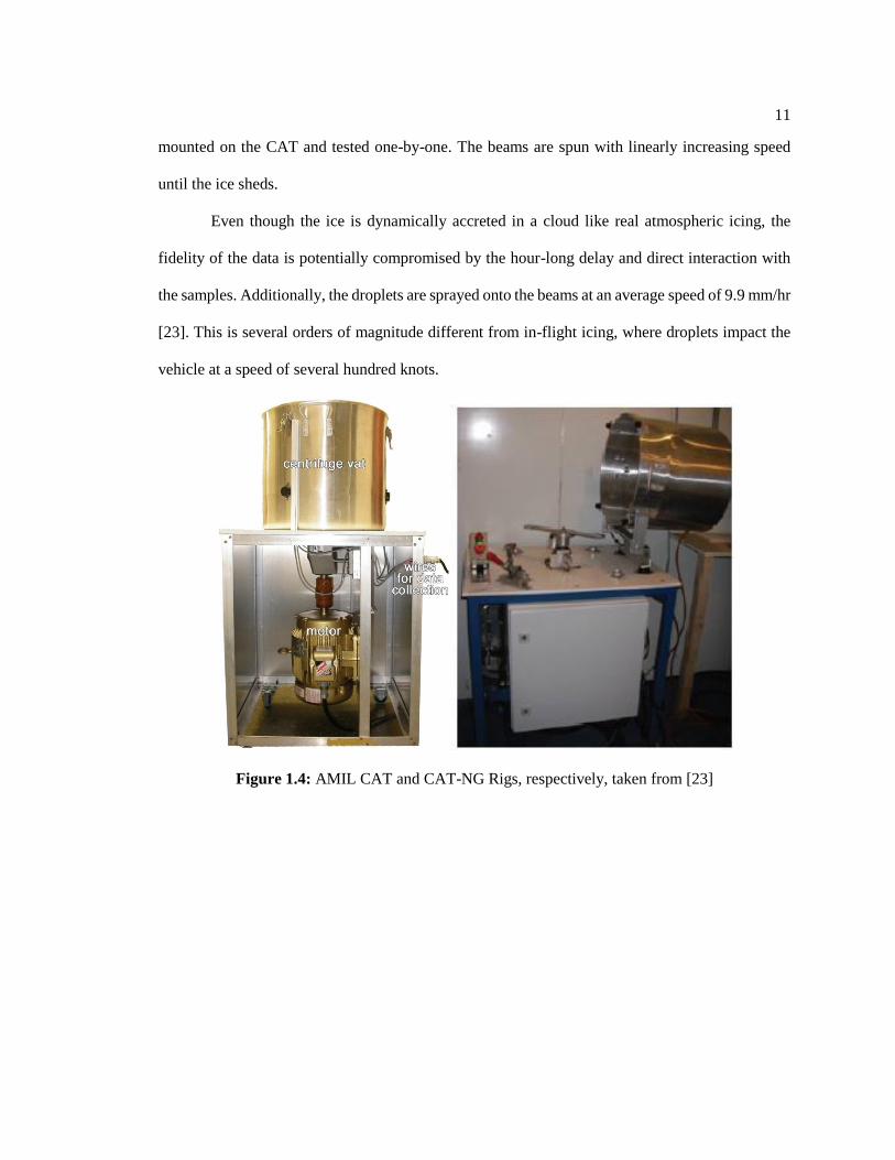
The other notable standard CAT rigs at the AMIL facility are shown in Figure 1.4. Both
consist of a motor that spins aluminum beams inside a vat. Several aluminum beams, which may
be coated with candidate ice-resistant coatings, are simultaneously sprayed with ice inside a
climatic chamber. Then the iced beams are left to chill for an hour before they are manually
11
mounted on the CAT and tested one-by-one. The beams are spun with linearly increasing speed
until the ice sheds.
Even though the ice is dynamically accreted in a cloud like real atmospheric icing, the
fidelity of the data is potentially compromised by the hour-long delay and direct interaction with
the samples. Additionally, the droplets are sprayed onto the beams at an average speed of 9.9 mm/hr
[23]. This is several orders of magnitude different from in-flight icing, where droplets impact the
vehicle at a speed of several hundred knots.
Figure 1.4: AMIL CAT and CAT-NG Rigs, respectively, taken from [23]

12
Figure 1.5: AMIL CAT Test Beams, taken from [23]
In a CAT test, the strain rate is proportional to both the angular speed and the angular
acceleration. (This relation will be derived in Chapter 3.) Fortin and Perron [23] found in their
study that the shear stress decreases with increasing strain rate, as shown in Figure 1.6.
Figure 1.6: Ice Failure Stress vs. Strain Rate in AMIL CAT Tests, taken from [23]
These findings are very interesting since the trend is the opposite of previously published strain
rate-adhesion strength studies.

13
1.5.2.2. Instrumented CAT
A prime example of an ICAT rig is the AERTS facility at Penn State. This rig tests full-
scale rotor blades inside an industrial freezer. The ceiling of the freezer contains an array of NASA
icing nozzles that spray a cloud as the rotor spins, just like AJ1. Photos are shown in Figure 1.7.
Figure 1.7: (a) Large AERTS ICAT Stand; (b) Rime Ice Feathers on AERTS Blade, taken from
Soltis et al. [12].
Centrifugal bending beams outfitted with strain gauges are mounted at the tip of the blades, as
shown in Figure 1.8. This configuration was first suggested by Stallabrass and Price in 1962 [24].
Figure 1.8: Schematic of Blade and Bending Beam. A full Wheatstone bridge of strain gauges,
insulated with epoxy, are outlined in red. Taken from Soltis et al. [12].

14
A sudden increase in voltage output from the strain gauge circuit indicates the ice has shed. The
voltage jump can be compared to the voltage drop when the bare rotor was initially brought up to
400 rpm from rest. This voltage ratio yields the centrifugal force required to shed the ice, and by
extension, the mass of ice that shed off [12]. Since the AERTS rig dynamically accretes impact ice
until it sheds off the surface, direct interaction with the ice is not necessary to obtain data.
1.6. Objectives
While most of the strain rate studies appear to agree, only the AMIL and AERTS centrifuge
tests use dynamically-accreted impact ice. Given that the correlation between strain rate and
adhesion strength is affected by the size and orientation of the ice grains, and that the ice crystal
structure is dictated by the freezing mechanism, it follows that strain rate studies for aircraft de-
icing purposes should be performed using impact ice. Additionally, if ice is to be removed passively
(via aerodynamic loading on fixed-wing vehicles or via centrifugal force on rotorcraft and wind
turbines), the ice must be tested in shear. This study aims to investigate whether the power
relationship between strain rate and adhesion strength of impact ice follows a similar trend as for
lab-grown ice. Additionally, temperature and surface roughness are varied to examine how strongly
they affect the trend. To these ends, the objectives of the present work include:
• Design and fabricate a small-scale ICAT rig (AJ2) for installation in a walk-in
freezer at NASA Glenn Research Center. Make the system hands-free to eliminate
direct interaction with the ice sample.
• Verify the ability of the system to perform standard liquid water content (LWC)
characterization and fixed-speed adhesion tests.
• Derive equations for finding ice adhesion strength and applied strain rate using
known variables from the strain rate tests.

15
• Perform experiments that vary the strain rate on the ice by applying different
acceleration rates. Compare the relationship between strain rate and shear adhesion
strength to previous studies.
1.7. Thesis Overview
The remainder of this paper is organized into the following chapters:
• Chapter 2: AERTS Jr. II Test Rig Design
The design specifications and safety analysis of the AJ2 rig are described.
• Chapter 3: Strain Rate Modeling on AJ2
Derivations are outlined for calculating strain rate and adhesion strength using Euler-
Bernoulli beam theory and strain gauge voltage readings.
• Chapter 4: Experimental Results of LWC and Fixed-Speed Adhesion Tests
Procedures and results for LWC characterization and fixed-speed adhesion tests are
presented.
• Chapter 5: Experimental Results of Strain Rate Adhesion Tests
Results for strain rate adhesion tests are presented and compared to results from
literature.
• Chapter 6: Conclusions and Recommendations for Future Work
Conclusions are drawn from the findings of the strain rate adhesion tests, and
suggestions for future studies are made.
16
Chapter 2
AERTS Jr. II Test Rig Design
2.1. Overview
“AERTS Jr. II,” henceforth referred to as “AJ2,” is an ICAT-type test rig designed and
constructed at Penn State University for the NASA Glenn Research Center. It consists of a
centrifuge rig, a control station, and a cloud spray system. Much like the full-scale AERTS facility
at Penn State, AJ2 uses on-rotor sensing and data acquisition to track the centrifugal force on impact
ice as it accretes, and the rig has the advantage of being portable like its predecessor, AJ1. AJ2 is
compact enough to fit inside any walk-in freezer, and its self-contained spray system allows for
icing tests to be performed outside of the AERTS chamber or the NASA IRT. Additionally, the
AJ2 motor driver allows the user to specify an acceleration rate when linearly ramping up to the
speed set-point. By varying the acceleration, the strain rate on the ice can be altered. This capability
also exists on the CAT rigs at the AMIL facility in Quebec; however, at AMIL the ice specimen is
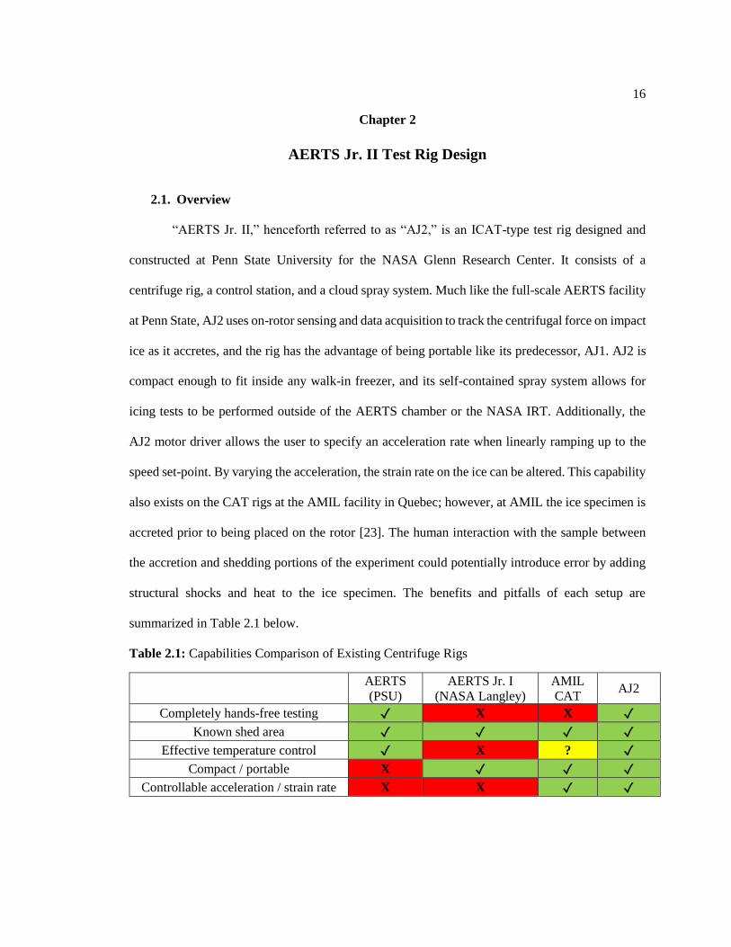
accreted prior to being placed on the rotor [23]. The human interaction with the sample between
the accretion and shedding portions of the experiment could potentially introduce error by adding
structural shocks and heat to the ice specimen. The benefits and pitfalls of each setup are
summarized in Table 2.1 below.
Table 2.1: Capabilities Comparison of Existing Centrifuge Rigs
AERTS
(PSU)
AERTS Jr. I
(NASA Langley)
AMIL
CAT AJ2
Completely hands-free testing ✓ X X ✓
Known shed area ✓ ✓ ✓ ✓
Effective temperature control ✓ X ? ✓
Compact / portable X ✓ ✓ ✓
Controllable acceleration / strain rate X X ✓ ✓

17
As can be seen in Table 2.1, AJ2 incorporates the best qualities of currently-existing CAT
rigs. It should be noted, however, that the temperature controllability in an AJ2 test depends entirely
on the quality of temperature control of the environment it is placed in, as AJ2 is only capable of
controlling the temperature of its own slip ring and spray nozzle.
This chapter will discuss the design and assembly of the AJ2 system. A simple schematic
is shown in Figure 2.1.
Figure 2.1: AJ2 in the Walk-In Freezer Configuration
In Figure 2.1, the control module is shown on the left, the cloud spray system is in the
center, and the rig inside the freezer is on the right. The motor driver regulates the electric current
to the rig motor inside the freezer. Signals from sensors on the rig and on the nozzle are relayed to
LabVIEW through a DAQ module. The LabVIEW program also regulates the pressure in the water
tank and in the nozzle air line. The following sections describe each of these AJ2 subsystems in
further detail.
2.2. Test Coupon Selection
The standard test coupons used on AJ2 were adopted from the Penn State AERTS facility,
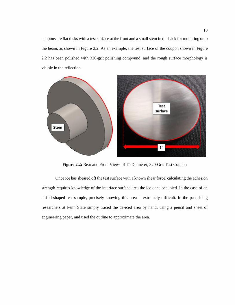
and the AJ2 rotor beams were designed with this predetermined coupon geometry in mind. The test
18
coupons are flat disks with a test surface at the front and a small stem in the back for mounting onto
the beam, as shown in Figure 2.2. As an example, the test surface of the coupon shown in Figure
2.2 has been polished with 320-grit polishing compound, and the rough surface morphology is
visible in the reflection.
Figure 2.2: Rear and Front Views of 1”-Diameter, 320-Grit Test Coupon
Once ice has sheared off the test surface with a known shear force, calculating the adhesion
strength requires knowledge of the interface surface area the ice once occupied. In the case of an
airfoil-shaped test sample, precisely knowing this area is extremely difficult. In the past, icing
researchers at Penn State simply traced the de-iced area by hand, using a pencil and sheet of
engineering paper, and used the outline to approximate the area.

19
Figure 2.3: Area Tracing on Deiced Airfoils (taken from Soltis et al. [12])
This method was difficult and imprecise. The new AERTS coupons are flat, allowing for exact
knowledge of the de-iced area without any human interaction.
The flatness of the coupon surface also serves another important purpose: it is conducive
to sanding, polishing, and application of so-called “ice-phobic” coatings for testing. Achieving a
uniform surface finish or coating application on airfoil-shaped geometry is significantly harder than
for flat plates.
Flat coupon geometry also increases the relevancy of test results to many different cases
and decreases collection efficiency variation across the surface. With a flat plate geometry, baseline
test results can be globally applied to materials, and the ice behavior is not unique to one specific
airfoil. The droplet collection efficiency of an object traveling through an icing cloud is heavily

20
geometry dependent. In general, the collection efficiency of wings and other airfoil-shaped objects
is dictated largely by the leading-edge radius of curvature [27]; the smaller the radius, the higher
the collection efficiency.
In theory, an infinitely large flat plate in icing conditions could be modeled as having a
radius of curvature of infinity and thus a collection efficiency of zero. However, the AJ2 coupons
are not infinitely large; they have an edge that permits airflow around the coupon. It is interesting
to note that the edges of the coupon have a higher collection efficiency than the center. This is
evidenced by the fact that some of the ice samples accreted on AJ2 appeared to be slightly “donut-
shaped,” as shown in Figure 2.4.
Figure 2.4: Examples of High Collection Efficiency at Coupon Edges (Rime ice on left, Glaze on
right)
Having established that the ideal test coupons for baseline adhesion testing on surfaces and
coatings should be flat, it is also crucial that the coupons be round on the edges. The test surfaces
on the AMIL facility are rectangular flats. If the iced area has corners, the corners have a different
collection efficiency than the coupon center or flat edges. On AERTS coupons, all locations around
the edge theoretically have the same collection efficiency. Additionally, as the ice undergoes kinetic
heating, convective cooling, and droplet impact, the ice shape is liable to undergo at least a small

21
amount of thermal expansion or contraction. This presents a problem for rectangular coupons, since
corners act as stress concentration points in the ice, and will likely weaken the ice as it slightly
expands and contracts. It is for these reasons that round, flat test coupons were selected for AJ2
tests.
2.3. Rotor Design
The rotor head was designed with modular “arms” or “beams” for holding the test coupons,
as shown in Figure 2.5 below. The arms are removable and inexpensive to manufacture, so other
geometries could also be tested if desired. The center of the flat test coupon is located at a radius
of 7.04 inches from the axis of rotation. At a maximum recommended motor speed of 5000 rpm,
the impact velocity seen by the test surface is approximately 307 feet per second (93.6 m/s). In
Figure 2.5 a passive balancer can also be seen mounted concentric with the rotor head. The
rectangular ballistic wall around the rotor was made of steel, and was designed to prevent injury
and damage in case one of the metal test coupons gets flung off.
Figure 2.5: Rotor Head with Beams and Passive Balancer
22
The beams, which are the main components of interest, will be discussed in greater detail
in Section 2.4.1.
2.3.1. Passive Balancing
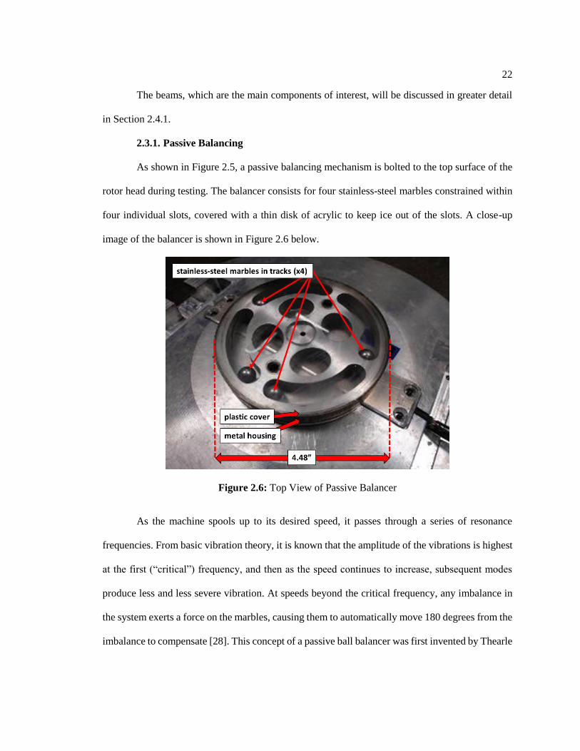
As shown in Figure 2.5, a passive balancing mechanism is bolted to the top surface of the
rotor head during testing. The balancer consists for four stainless-steel marbles constrained within
four individual slots, covered with a thin disk of acrylic to keep ice out of the slots. A close-up
image of the balancer is shown in Figure 2.6 below.
Figure 2.6: Top View of Passive Balancer
As the machine spools up to its desired speed, it passes through a series of resonance
frequencies. From basic vibration theory, it is known that the amplitude of the vibrations is highest
at the first (“critical”) frequency, and then as the speed continues to increase, subsequent modes
produce less and less severe vibration. At speeds beyond the critical frequency, any imbalance in
the system exerts a force on the marbles, causing them to automatically move 180 degrees from the
imbalance to compensate [28]. This concept of a passive ball balancer was first invented by Thearle
23
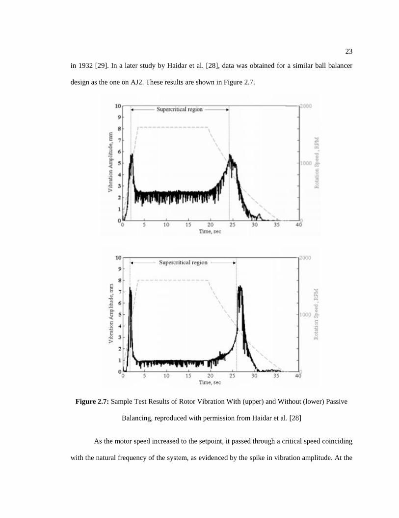
in 1932 [29]. In a later study by Haidar et al. [28], data was obtained for a similar ball balancer
design as the one on AJ2. These results are shown in Figure 2.7.
Figure 2.7: Sample Test Results of Rotor Vibration With (upper) and Without (lower) Passive
Balancing, reproduced with permission from Haidar et al. [28]
As the motor speed increased to the setpoint, it passed through a critical speed coinciding
with the natural frequency of the system, as evidenced by the spike in vibration amplitude. At the

24
steady-state speed, higher than the critical speed, the addition of the balancer significantly reduced
the vibration amplitude from 2.5 mm to 1 mm. The vibration amplitude spiked again as the motor
decelerated.
The balancer on AJ2 has 412 g-mm, or 16.2 g-in of balancing authority. Knowing the radius
to the coupon center is 7.04 inches, the balancer can compensate for 2.3 grams of imbalance at the
beam tip. The amount of ice that typically accretes on a coupon during strain rate tests is 1-3 grams,
so this balancer is extremely useful for uneven ice shedding at high speeds. By allowing the rotary
system to self-correct potential imbalances, the passive balancer improves the safety of the rig and
will likely increase its longevity.
2.3.2. Rotor Design Improvements
Several components of AJ2 underwent multiple design iterations, but the two most notable
improvements occurred on the rotor: namely, altering the angle of the bending beam and the
geometry of the shield plate. The initial and final design of these components are shown in Figure
2.8.
Figure 2.8: Initial (left) and Final (right) Design Iterations of Beam Assembly

25
2.3.2.1. Angled Rotor Beams
The original arm design for AJ2 had a 90˚ angle between the trunk and the bending beam
itself, as shown in the left photo of Figure 2.9. This was for simplicity of manufacturing and to
keep the geometry as close to the cantilever beam assumption as possible. However, after several
months of testing, it became clear that the beams needed to be bent inward towards the rotor, for
aerodynamic purposes and to better resolve the shear force on the ice.
Figure 2.9: Photos of the Right-Angle and Inward-Facing Beams
An extreme example of bridging that occurred while testing with the original right-angle
beams is shown in Figure 2.10 below. “Bridging” is when the ice accreted on the coupon is
connected to other ice on the beam or on the rotor. If ice in other locations is preventing the ice on
the coupon from shedding, the adhesion data cannot be trusted. It is clear from the orientation of
the ice shape that the velocity vectors of the droplets impacting the test surface were not normal to
the surface; they were tangent to the rotation, which is to be expected. As a result, ice was bridging
from the test surface to the coupon rim and the inside of the bending beam. The adhesion results

26
from a test like this would be unacceptable because the ice would need to overcome both adhesion
and cohesion forces to shed.
Figure 2.10: Rime Ice Bridging from the Beam to the Coupon on a Right-Angle Beam
Figure 2.11 highlights a second flaw with the right-angle beam design. The angle between
the coupon surface and the radius vector was originally 14.4˚. Consequently, the centrifugal force
was not loading the ice in pure shear; there was a peeling effect as well. This is not ideal for tests
designed to isolate adhesion strength of ice in pure shear. The beams were redesigned to be angled
inwards, as shown in Figure 2.9; in the new bent beam design, the coupon surface angle differs
from the radius vector by only 1.2˚. After the new beams were installed, ice grew normal to the test
surface, as desired, and no more ice accreted around the rim of the coupons.

27
Figure 2.11: Diagram of Centrifugal Force Vector Correction
2.3.2.2. Shield Plates
The purpose of the shield plates over the root of the t-inserts was twofold: to protect the
soldered strain gauge and thermistor joints from moisture, and to prevent the t-inserts from coming
out of place (which is highly unlikely). As shown previously in Figure 2.8, the shield plates were
originally designed as simple rectangular plates with bolt holes. However, as shown in Figure 2.12,
the leading edge of the plate disrupted airflow over the rotor as it spun, causing ice buildup on the
corner. In Figure 2.10, which was in a rime icing condition, the corner was simply a place where
large ice feathers formed. In the glaze condition, however, the blunt corner caused more severe
issues because the water travelled radially outwards before freezing, sometimes causing bridging
between the coupon and the rotor, as shown in Figure 2.12.

28
Figure 2.12: Glaze Ice Bridging from the Corner of the Original Shield Plate to the Coupon
The solution to this problem simply required the plates to be modified with a more
aerodynamic geometry. A chamfer was added to the leading edge of the plate, and the outer half of
the plate was filed down to conform closer to the rotor geometry, as shown in Figure 2.8. This small
change eliminated the issues seen with the original shield plate.
2.4. DAQ
For data acquisition, a similar approach was used as the main AERTS facility. Strain and
temperature readings from the rotor beams were relayed from the rotating frame to the fixed frame
through the slip ring, as shown in Figure 2.13.

29
Figure 2.13: Shaft Assembly
The rotor signals, as well as the ones from the Hall sensor and plumbing system, were
recorded and displayed real-time using a LabVIEW virtual instrument.
2.4.1. On-Rotor Measurements
A close-up view of the instrumented rotor arm is shown in Figure 2.14.

30
Figure 2.14: Instrumented Rotor Arm
Half-bridge strain gauges were mounted on the inner and outer surface of each arm,
forming a full Wheatstone bridge, as shown in Figure 2.15.
Figure 2.15: Diagrams of the Wheatstone Bridge Circuit (left) and the Placement on the Beam
(right) [30]
This configuration measures bending strain due to centrifugal force. The output voltage
from the strain gauges, V0, is amplified and passed down through the slip ring to the DAQ module.
Similarly, the thermistor output voltages, V1 and V2, are compared to the excitation voltage V+ to
approximate the coupon temperature. A diagram of these circuits is shown in Figure 2.16.

31
Figure 2.16: Diagram of On-Rotor Measurements
2.4.2. Static Measurements
In addition to signals from the on-rotor sensors, the DAQ module also collects data from
the Hall sensor mounted on the motor frame, and from the pressure transducers on the nozzle
assembly. The spray system will be discussed in Section 2.5.2.
The Hall sensor emits a positive reading when it is in close proximity to a magnet. Four
magnets are mounted 90˚ from each other on the underside of the rotor head, as shown in Figure
2.17. Also visible are small indents that were drilled when the rotor was sent off to get
professionally balanced.

32
Figure 2.17: Underside of the Rotor
To be able to accurately sample the speed using the Hall sensor, the minimum required
sampling rate in LabVIEW was dictated by the Nyquist frequency, as seen in Equation (2.1).
6000 𝑟𝑒𝑣
𝑚𝑖𝑛∗
1 𝑚𝑖𝑛
60 𝑠𝑒𝑐∗
4 𝑝𝑜𝑖𝑛𝑡𝑠
𝑟𝑒𝑣∗ 2 = 800 𝐻𝑧 (2.1)
With the processing power of the selected computer, it was determined that the
LabVIEW VI could easily sample data at a frequency of 8000 Hz, which is 10x more than
necessary to resolve the speed. Calculation of the Nyquist frequency provided confidence that the
selected sampling rate was more than adequate.
2.4.3. User Interface
The layout of the LabVIEW front panel, with which the user interacts with the system, can
be seen in Figure 2.18.

33
Figure 2.18: LabVIEW Front Panel

34
The panel in the top left corner contains the data-saving options. Below that is the water
and air nozzle switches and pressure control. The graph in the top right corner displays the target
and current MVD of the cloud, calculated from the pressure transducers in the nozzle. The bottom
panels of the user interface show the motor speed and plots of the strain gauge voltages and on-
beam temperatures.
Over the course of each test, the LabVIEW program writes the values of all the recorded
parameters, including coupon temperatures, strain gauge voltages, air and water pressures,
calculated MVD, and motor speed, to text files in a user-specified location.
In the early stages of troubleshooting the AJ2 rig, spinning the motor introduced excessive
noise in signals that had to be relayed through the slip ring (namely, the thermistors and strain
gauges). After the electrical panel was grounded to the motor power ground and two
electromagnetic interference filters were added to the strain gauge lines inside the electrical box,
the noise was greatly reduced, though some low-amplitude noise remains.
2.5. Cloud Spray System
2.5.1. Plumbing
When AJ2 is mounted in the Icing Research Tunnel, the user will simply use the calibrated
icing cloud generated by the spray bars in the IRT. However, when the unit is used in a walk-in
freezer, an air and water regulation system is needed to generate an icing cloud that is representative
of atmospheric flight.

35
Figure 2.19: AJ2 Plumbing Panel and Electrical Box Containing the DAQ System
As can be seen in Figure 2.19, a shop air hose gets connected at the top of the plumbing
assembly. If the air input valve is set to open, the air will travel through two pressure regulators.
On the AERTS Jr. I machine, all the valves and regulators for the plumbing system were manual,
but in the redesign, the valves and regulators are all controlled electronically via LabVIEW, further
making AJ2 a “hands-free” system. On the panel, the regulator on the right side controls the air
pressure into the icing cloud nozzle, while the regulator on the left side controls the pressure inside
the water tank by allowing shop air to fill the top of the tank. When the water valve is open,
pressurized water will flow from the bottom of the tank into the cloud nozzle. A bypass valve
allows air to flow through the water line between tests to prevent any stagnant water from freezing
and clogging the nozzle between tests. The LabVIEW user interface is programmed to allow the

36
user to open and close valves and change the air pressure and desired MVD. The program also
prevents the bypass and water valves from being set to “open” at the same time.
2.5.2. Nozzle Assembly
Figure 2.20 shows the cloud nozzle assembly that is embedded in the walk-in freezer
ceiling. In the nozzle assembly, which is connected to the plumbing assembly panel by hoses, two
pressure transducers measure the pressure in the air and water lines and send the data to the DAQ
module. The pressure transducers allow the LabVIEW program to calculate and display, in real
time, the current MVD of the cloud.
Figure 2.20: Icing Cloud Nozzle Assembly
The pressure differential between the air and the water in the nozzle is crucial for producing
the target MVD of the cloud, so it is important to have these transducers as close to the nozzle as
possible. This entire assembly will be embedded vertically in the ceiling of the walk-in freezer at
the NASA Glenn Research Center RIMELab. Figure 2.21 below shows the nozzle in closer detail.
The nozzle is an official NASA icing cloud nozzle with air input on the side and water input in the

37
back, as shown in Figure 2.21. To avoid nozzle freezing issues, heaters controlled by a PID
temperature controller will maintain the nozzle at a user-specified temperature. The nozzle
temperature control module is located on the front panel of the electrical box.
Figure 2.21: Close-up of AJ2 Icing Nozzle
On the LabVIEW front panel shown in Figure 2.18, the user selects the desired air pressure
and target MVD, and a PID controller within LabVIEW automatically regulates the air and tank
pressure to achieve the target MVD. It calculates the current MVD in real-time based on the nozzle
pressure transducers and self-corrects accordingly. The rectangular nozzle housing can be used for
both “Standard” and “Mod1” NASA nozzles. The two different types of nozzles are useful for
simulating different types of clouds. On AJ2, the user must simply screw the desired nozzle type
into the housing and select either “Standard” or “Mod1” from the nozzle drop-down menu on the
LabVIEW front panel. This selection dictates which set of equations will be used by the MVD PID
controller:
𝑀𝑉𝐷𝑠𝑡𝑎𝑛𝑑𝑎𝑟𝑑 =a+b(𝑃𝑎𝑖𝑟)+c(𝑃𝑎𝑖𝑟)2+d∗ln(∆P)
1+e(𝑃𝑎𝑖𝑟)+f(𝑃𝑎𝑖𝑟)2+g(𝑃𝑎𝑖𝑟)3+h∗ln(∆P) (2.2)
𝑀𝑉𝐷𝑀𝑜𝑑1 = a + b(𝑃𝑎𝑖𝑟)𝑐 + d(∆P)𝑒 + f(𝑃𝑎𝑖𝑟)𝑐(∆P)𝑒 (2.3)
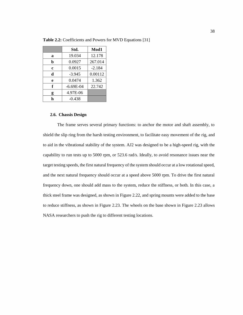
where the values of the constants a through h are listed in Table 2.2.
38
Table 2.2: Coefficients and Powers for MVD Equations [31]
Std. Mod1
a 19.034 12.178
b 0.0927 267.014
c 0.0015 -2.184
d -3.945 0.00112
e 0.0474 1.362
f -6.69E-04 22.742
g 4.97E-06
h -0.438
2.6. Chassis Design
The frame serves several primary functions: to anchor the motor and shaft assembly, to
shield the slip ring from the harsh testing environment, to facilitate easy movement of the rig, and
to aid in the vibrational stability of the system. AJ2 was designed to be a high-speed rig, with the
capability to run tests up to 5000 rpm, or 523.6 rad/s. Ideally, to avoid resonance issues near the
target testing speeds, the first natural frequency of the system should occur at a low rotational speed,
and the next natural frequency should occur at a speed above 5000 rpm. To drive the first natural
frequency down, one should add mass to the system, reduce the stiffness, or both. In this case, a
thick steel frame was designed, as shown in Figure 2.22, and spring mounts were added to the base
to reduce stiffness, as shown in Figure 2.23. The wheels on the base shown in Figure 2.23 allows
NASA researchers to push the rig to different testing locations.

39
Figure 2.22: Diagram of the Test Stand and Frame
Figure 2.23: Base Frame of the AJ2 Rig
2.6.1. Motor Selection
The dimensions of the rig chassis were guided by the size of the motor. As a first step to
selecting a motor, a preliminary power estimate was calculated:

40
𝑃𝑜𝑤𝑒𝑟𝑟𝑒𝑞𝑢𝑖𝑟𝑒𝑑,𝑚𝑜𝑡𝑜𝑟 = (𝐼𝑟𝑜𝑡𝑜𝑟𝛼)𝜔 (2.4)
The moment of inertia of the rotor head assembly was found in SolidWorks mass properties
to be 6.533E-2 slug-ft2. To allow for some leeway in the speed range, the operating speed was set
at 6000 rpm. Since strain rate testing requires high acceleration rates, the angular acceleration was
set to 500 rpm per second. This yields a minimum required horsepower of 3.91 hp. This assumes
that the motor is 100% efficient at converting electrical to mechanical energy, and neglects added
friction from the rest of the components attached to the shaft. Induction motor engineers at Baldor
Motors were consulted about selecting a motor to meet the unique design requirements of the test
rig, such as thrust bearings to withstand heavy axial loads, and environmental protection to
withstand the extreme cold and moisture. The engineers from Baldor recommended a 6 hp motor
with a driver capable of controlling the acceleration rate.
2.6.2. Fairing
To facilitate optional mounting in the NASA Icing Research Tunnel, the rig’s base frame
has been modified to fit the IRT turntable and mounting hardware, as specified in Soeder et al. [32]
and in accordance with NASA wind tunnel safety standards. Airfoil-shaped ribs support a sheet
metal shell that makes the rig more aerodynamic in a forward-flight test condition. The ribs are
visible in Figure 2.24.

41
Figure 2.24: CAD Model of the Fairing Ribs
Analysis of the fairing will be discussed further in Section 2.7.3.
2.7. NASA Safety Analysis
Since AJ2 was developed for NASA Glenn using federal funding, it was necessary to prove
that the rig satisfied certain safety requirements as outlined by the customer. The safety
specifications in this case were taken from the GRC Containment Design Guide. It is clear from
the content that the Design Guide was primarily geared toward multi-bladed turbomachinery
components, such as compressor and turbine rotor disks. Nevertheless, the relevant principles and
regulations were applied to the AJ2 rotor where appropriate. In total, three different analyses were
performed to show that AJ2 could be safely used at NASA: a stress analysis of the beams, ballistic
wall thickness calculations, and fairing drag calculations to validate the IRT floor mount
configuration.
Even though the AJ2 motor is rated for 6000 rpm, it was decided that the operating speed
during testing should be limited to 5000 rpm. This decision followed the failure of one strain gauge
assembly under centrifugal loads at 5000 rpm, as shown in Figure 2.25.

42
Figure 2.25: Failure of Marine Epoxy
It should be noted that the failure of the marine epoxy may have been caused by any number
of factors, including high strain rate (acceleration of 100 rpm per second in that test), fatigue, or
thermal expansion, but for the sake of being conservative, 5000 rpm seemed like an appropriate
limit to set. Thus, all following safety analysis was performed assuming operation at the maximum
recommended speed of 5000 rpm.
2.7.1. Beam Yielding
An FEA analysis of the rotor head assembly was performed in SolidWorks to ensure that
the beams would not yield under the centrifugal loads. A simulated cylindrical ice mass of 1”
diameter and 1” thickness was modeled and attached to the coupon face. Since ice material
properties are highly variable, SolidWorks does not have ice in its materials database. Therefore,
the cylinder was specified to have the density of water (1000 kg/m3), which is a conservative
estimate since most ice contains air pockets.
A centrifugal load was applied radially outward from the axis of rotation. The center of
rotation of the rotor was given a “fixed” boundary condition, and the underside of the rotor was
specified as having a “roller” boundary condition. These boundary conditions prevented the rotor

43
from translating in 3D space but allowed it to deform outwards. The resulting contour plot is shown
in Figure 2.26.
Figure 2.26: Contour Plot of von Mises Stress in Rotor Assembly at 5000 rpm
The maximum stress locations were on the inside corner of the beam, and inside the
through-hole designed for passing strain gauge wires through the beam.
Section 1.14.3.1 of the Containment Design Guide requires a yield safety factor of 1.1 and
an ultimate safety factor of 1.5 [33]. The inside corner of the beam experiences both shear stress
and tensile stress. Therefore, it was decided that the safety factors should be calculated using the
von Mises stress. The von Mises stress, which is calculated using a combination of all six normal
and shear stress components, allows structures under complex loading conditions to be compared
to the yield strength of a material in pure tension [34].
According to SolidWorks, the maximum von Mises stress in the assembly was determined
to be 199 MPa. From ASM [35], the tensile yield strength of 6061 aluminum is 276 MPa, and the
tensile ultimate strength is 310 MPa. This means that for beams spinning at 5000 rpm with 1” thick

44
non-porous ice, the yield safety factor is 1.38, and the ultimate safety factor is 1.55, which satisfies
NASA’s requirements. It should also be noted that an ice thickness of 1” is a conservative estimate,
since ice observed during high-speed AJ2 adhesion tests rarely exceeds 0.5”.
The test coupons were also examined in the simulation to ensure the accretion surface
would not shear off the stem. Since the coupons are made of stainless steel, the coupon yield safety
factor was 7.9. The beams would fail long before the coupons would. Additionally, the Design
Guide describes how to protect against a “hub burst”—in other words, the solid rotor itself
fragmenting into multiple pieces. However, the rotor is so thick that the stresses inside it were
negligible, making a hub burst extremely unlikely.
2.7.2. Ballistic Wall Calculations
According to Section 1.14.4.2.1 of the Containment Design Guide [33], a ballistic wall
around rotating machinery must be sufficiently thick to withstand shedding of “blade fragments,”
or in this case, test coupons and ice. These calculations did not require FEA simulations, only
knowledge of the mass values shown in Table 2.3.
Table 2.3: Mass Values for Possible Projectiles
Approx. mass of 1" thick ice puck 13 g
Approx. mass of single coupon 18 g
Approx. mass of single beam, broken at root of bending 30 g
SUM 61 g
The original ballistic wall, seen previously in Figure 2.5, is rectangular and made of 0.25”
thick steel. In the Design Guide, the required mild steel shield thickness is plotted as a function of
the kinetic energy of a projectile. The calculated projectile energy at different levels of failure of
the AJ2 rotor assembly are shown in Table 2.4.

45
Table 2.4: Kinetic Energy Associated with Levels of Rotor Failure
KINETIC ENERGY @ 5000 rpm
1" ICE AND SINGLE COUPON SHED 1205 in-lbf
1" ICE, COUPON, AND BEAM BREAK 2371 in-lbf
BOTH BEAMS BREAK 4743 in-lbf
The green, yellow, and red levels of projectile energy have been superimposed on the plot
from the Design Guide. The purple horizontal line indicates a shield thickness of 0.25”.
Figure 2.27: Graph of Required Mild Steel Shield Thickness vs. Projectile Energy [33]
As evidenced by Figure 2.27, a mild steel ballistic wall with thickness of 0.25" (or thicker)
contains single arm breakage with "Zone 4" safety level and contains dual arm breakage well into

46
"Zone 3" safety level. According to the zone definitions, this means that NASA personnel could
safely be in the freezer or wind tunnel while AJ2 is running at 5000 rpm, if the ballistic wall is up.
Although the original ballistic wall in Figure 2.5 was proven to be thick enough, it still
does not totally satisfy NASA criteria. The Design Guide also stipulates that ballistic walls must
be round in nature, containing no sharp corners. This is to ensure that the ballistic wall will behave
the same regardless of where the projectile hits. NASA was concerned that the corner brackets of
the original ballistic wall could be weak points, so the ballistic wall needed to be redesigned. A
CAD model of the new and improved ballistic wall is shown in Figure 2.28.
Figure 2.28: CAD Model of AJ2 rig with Elliptical Ballistic Wall
The round ballistic wall will be in use when the rig is in its freezer configuration. When it
is installed in the Icing Research Tunnel, however, the fairing will be installed instead. GRC
engineers stated that the walls and windows of the IRT were strong enough to act as a ballistic wall
in the IRT configuration.
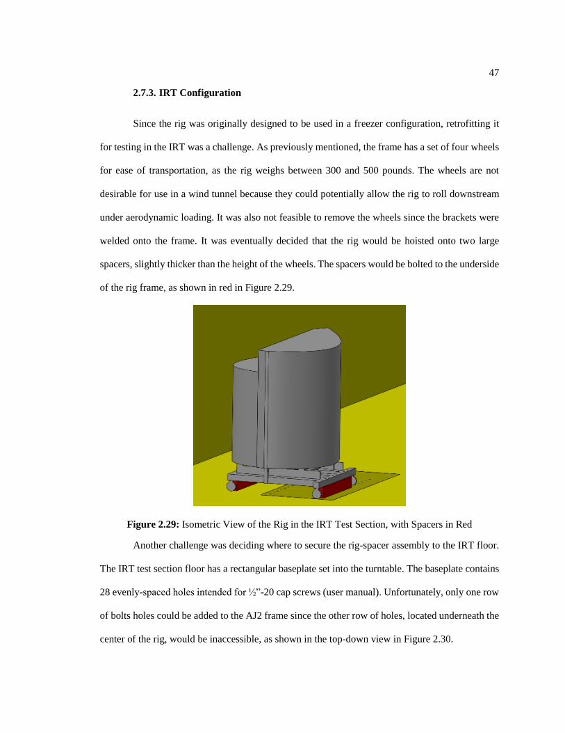
47
2.7.3. IRT Configuration
Since the rig was originally designed to be used in a freezer configuration, retrofitting it
for testing in the IRT was a challenge. As previously mentioned, the frame has a set of four wheels
for ease of transportation, as the rig weighs between 300 and 500 pounds. The wheels are not
desirable for use in a wind tunnel because they could potentially allow the rig to roll downstream
under aerodynamic loading. It was also not feasible to remove the wheels since the brackets were
welded onto the frame. It was eventually decided that the rig would be hoisted onto two large
spacers, slightly thicker than the height of the wheels. The spacers would be bolted to the underside
of the rig frame, as shown in red in Figure 2.29.
Figure 2.29: Isometric View of the Rig in the IRT Test Section, with Spacers in Red
Another challenge was deciding where to secure the rig-spacer assembly to the IRT floor.
The IRT test section floor has a rectangular baseplate set into the turntable. The baseplate contains
28 evenly-spaced holes intended for ½”-20 cap screws (user manual). Unfortunately, only one row
of bolts holes could be added to the AJ2 frame since the other row of holes, located underneath the
center of the rig, would be inaccessible, as shown in the top-down view in Figure 2.30.

48
Figure 2.30: Top-Down View of the AJ2 Mounting Location with Respect to the IRT Test Section
It was therefore necessary to analyze the drag force on the test rig, to ensure that the eight
½” bolts could withstand the unbalanced shear forces.
The flow conditions inside the IRT test section during an AJ2 experiment are very complex.
A full CFD simulation intended to capture all the flow dynamics, especially with a spinning rotor,
would need to be 3-D, unsteady, viscous, turbulent, and rotational in some regions. The magnitude
of such a simulation would be a research project in and of itself. Therefore, a simplified
aerodynamic statics analysis has been performed to estimate the ability of the bolts to withstand
the loading.
The fairing geometry was tailored to the dimensions of the already-existing rig. As such, it
is not a recognized airfoil shape, so the drag coefficient is unknown. However, as can be seen in
Figure 2.31, the maximum thickness of the so-called “airfoil” is almost exactly double the leading-
edge radius—it resembles a circle with a tail. In other words, the geometry can be conservatively
approximated as a cylinder in cross-flow. The added drag of treating the “airfoil” like a cylinder
helps make up for the fact that the extra drag at the frame base and around the rotor is being ignored.

49
This analysis, while very simplistic, will provide a ballpark estimate of the magnitude of forces the
floor bolts can be expected to withstand.
Figure 2.31: Dimensioned View of Streamlined Circular Fairing Shell
To find the drag coefficient, the Reynolds number must first be calculated. The Reynolds
number is evaluated at an airspeed of 50 kts, the minimum velocity required to achieve a uniform
icing cloud in the IRT test section.
𝑅𝑒 =𝜌𝑎𝑖𝑟∗𝑈∗𝐷𝑐𝑦𝑙
𝜇𝑎𝑖𝑟=
(1.225 𝑘𝑔
𝑚3)(25.722𝑚
𝑠)(0.848 𝑚)
(1.73×10⁻⁵ 𝑘𝑔
𝑚∙𝑠)
= 1.545 × 10⁶ (2.5)
According to Cengel and Cimbala [36], for Reynolds numbers above 104, the drag
coefficient of a cylinder in cross-flow is 1.2 for laminar flow and 0.3 for turbulent flow. For the
sake of being conservative, laminar flow will be assumed. The frontal area will be taken to be the
diameter 0.848 m multiplied by the distance between the tunnel floor and the fairing top, 1.181 m.
Drag =1
2𝜌𝑎𝑖𝑟𝐶𝐷𝐴𝑓𝑟𝑜𝑛𝑡𝑎𝑙𝑈2
= (0.6) (1.225 𝑘𝑔
𝑚3) (0.848 ∗ 1.181 𝑚2) (25.722𝑚
𝑠)
2= 487.0 𝑁 (2.6)

50
Therefore, assuming the amount of drag on the fairing is similar to a cylinder in cross-flow,
there will be approximately 487 N of force, or 110 lbf. The highest shear force will be on the final
downstream bolt in the line. Not only will it need to withstand the downstream drag force, but it
will also need to withstand the clockwise moment imposed on the frame.
To approximate the highest expected force in the most heavily-loaded bolt, the frame was
reduced to a simple statics problem, with the drag force acting on the stagnation point of the fairing,
and with no other bolts carrying any force in the flow direction. If a single bolt can withstand these
forces, the series of eight bolts will certainly not fail.
Figure 2.32: Free-Body Diagram of Simplified Statics Analysis on Rig Frame

51
From the three equilibrium equations, it was determined that the resultant force on the final
bolt is 140.2 lbf. A bolt cannot be treated the same as a solid rod, so to find the effective shear area,
Equation (2.7) [37] must be used.
𝐴𝑠ℎ𝑒𝑎𝑟,𝑏𝑜𝑙𝑡 = 0.7854 [𝐷𝑏𝑜𝑙𝑡 −0.9743
(# 𝑡ℎ𝑟𝑒𝑎𝑑𝑠 𝑝𝑒𝑟 𝑖𝑛)]
2= 0.7854 [0.5 −
0.9743
20]
2 (2.7)
For ½”-20 bolts, the effective shear area is 0.160 sqin. Therefor the resultant shear stress
in the last bolt is 876.5 psi. According to the handbook from the Specialty Steel Industry of North
America [37], the allowable shear stress in type 304 and 306 stainless steel bolts is 10.5 ksi. Since
the last bolt in the set can withstand the shear forces with such a high safety factor, it is safe to
assume none of the eight bolts will shear for IRT testing in a 50 kt flight condition.

52
Chapter 3
Strain Rate Modeling on AJ2
Strain rate adhesion tests on AJ2 are performed in a similar fashion to the AERTS fixed-
speed adhesion tests, but with some key differences. In a fixed-speed test, the icing cloud is sprayed
until a shedding event occurs. In a strain rate test, the cloud is purposely stopped before the ice can
shed, so that the effects of rotational acceleration can be examined. After a certain amount of time,
the spray is deactivated; then the motor speed is ramped up at a known linear rate until the ice
sheds. The chosen acceleration rate and the speed at which the ice finally sheds determine the strain
rate.
Figure 3.1 is an example of what the strain gauge signals look like over the course of a
strain rate test.
Figure 3.1: Sample Graph of Strain Gauge Output Voltage Throughout Strain Rate Adhesion Test
In previous strain rate-adhesion strength experiments found in literature, scientists
frequently used some combination of load cells, weights, linear actuators, and displacement sensors
to track the stress and strain experienced by a lab-grown ice specimen of known dimensions. Stress

53
was determined by simply dividing the applied force over the wetted area, and strain was found
from dividing displacement by the original specimen length.
The fact that AJ2 is a rotary system that accretes ice dynamically adds significant
complexity to the calculation of strain rate and adhesion strength values. It was therefore necessary
to derive equations that related the voltage output from the AJ2 strain gauges, to the mass of
accreted ice and, by extension, the centrifugal force required to shear the ice off the test coupon.
This chapter will detail the derivation of the equations used to process the AJ2 test data.
The arms on the AJ2 rotor head were treated as cantilever beams, as shown in Figure 3.2.
Figure 3.2: Close-Up Photo of AJ2 Rotor Head with Bending Arms (left), and Cantilever Beam
Free-Body Diagram (right)
In Figure 3.2 the centrifugal force on the test coupon and ice is represented as a point force,
P, at the beam tip. Distributed force Q is the centrifugal load acting on the mass of the beam itself.
The values of P and Q are evaluated in Equations (3.1) and (3.2) below.
𝑃 [𝑁] = (𝑚𝑐𝑜𝑢𝑝𝑜𝑛 + 𝑚𝑖𝑐𝑒)(𝑟𝑡𝑖𝑝,𝑏𝑒𝑎𝑚)(𝜔2) (3.1)
𝑄 [𝑁/𝑚] = (𝑏ℎ ∗ 𝜌𝐴𝑙 6061)(𝑟𝑎𝑣𝑔,𝑏𝑒𝑎𝑚)(𝜔2) (3.2)
Since the beam is not curved, technically the radius r used to calculate centrifugal force
does not stay constant throughout the entire beam. However, the beam is angled inwards towards

54
the circular rotor, such that the beam is nearly tangent to the rotor. Therefore, the radial distances
between the center of rotation and the beam root (rroot), and the center of rotation and the beam tip
(rtip), vary by less than 2 percent. For this reason, in this analysis the average (ravg) of the two values
is used for the centrifugal force Q on the beam. These definitions are displayed more clearly in
Figure 3.3.
Figure 3.3: Radius Label Convention
If the beam is split at some arbitrary lengthwise location X, as in Figure 3.4, and a force
and moment balance is evaluated, the equations for shear and moment at every lengthwise location
can be found. The sign convention is that positive shear acts in the “upwards” direction (towards
the rotor’s center of rotation), and positive moment creates a concave-up beam.

55
Figure 3.4: Shear and Moment Diagrams for the Bending Beam
Using Euler-Bernoulli beam theory to approximate the strain,
𝜀(𝑥, 𝑦) = −𝑦𝑀(𝑥)
𝐸𝐼𝑏𝑒𝑎𝑚 (3.3)

56
where 𝑦 =ℎ
2 for the inside (rotor side) of the beam and 𝑦 = −
ℎ
2 for the outside of the beam.
Since the strain gauges are assumed to be mounted directly at the root of the beam, the moment is
evaluated at x=0.
The tensile strain seen at the inside root of the beam can be expressed as:
𝜀(𝑥 = 0, 𝑦 = ℎ/2) = ℎ
2𝐸𝐼𝑏𝑒𝑎𝑚[𝑃𝐿 +
1
2𝑄𝐿2] (3.4)
Plugging in the earlier equations for P and Q and rearranging yields:
𝜀(𝑥, 𝑦) = ℎ𝜔2𝐿
2𝐸𝐼𝑏𝑒𝑎𝑚[(𝑚𝑐𝑜𝑢𝑝𝑜𝑛 + 𝑚𝑖𝑐𝑒)(𝑟𝑡𝑖𝑝,𝑏𝑒𝑎𝑚) +
1
2(𝑏ℎ ∗ 𝜌𝐴𝑙 6061)(𝑟𝑎𝑣𝑔,𝑏𝑒𝑎𝑚)𝐿]
= ℎ𝜔2𝐿
2𝐸𝐼𝑏𝑒𝑎𝑚[(𝑚𝑖𝑐𝑒𝑟𝑡𝑖𝑝,𝑏𝑒𝑎𝑚) + (𝑚𝑐𝑜𝑢𝑝𝑜𝑛𝑟𝑡𝑖𝑝,𝑏𝑒𝑎𝑚) +
1
2(𝑏ℎ ∗ 𝜌𝐴𝑙 6061)(𝑟𝑎𝑣𝑔,𝑏𝑒𝑎𝑚)𝐿] (3.5)
As Work and Lian pointed out in [13], on ICAT rigs two types of strain rates are observed.
The ice at the metal interface experiences an increase in strain in two ways: first due to the buildup
of additional ice mass, and secondly due to an increase in motor speed after the accretion phase is
over. This is shown in Figure 3.5, which shows a sample plot of strain gauge voltage output over
the course of a strain rate test.
Figure 3.5: Sample Graph of Strain Gauge Output Voltage Throughout Strain Rate Adhesion Test

57
During the first phase of strain rate testing, the rotational speed ω is held constant, while
the mass of the ice increases. While ice is accreting at a constant speed, the strain rate at the beam
root can thus be approximated as:
[𝑑𝜀
𝑑𝑡]
𝑎𝑐𝑐𝑟𝑒𝑡𝑖𝑜𝑛=
ℎ𝜔𝑠𝑡𝑒𝑎𝑑𝑦2𝐿𝑟𝑡𝑖𝑝,𝑏𝑒𝑎𝑚
2𝐸𝐼𝑏𝑒𝑎𝑚∗
𝑑𝑚𝑖𝑐𝑒
𝑑𝑡 (3.6)
It should be noted that as ice accretes on the coupon, the geometry is dynamic and so is the
collection efficiency. Even with no ice on the coupon, the collection efficiency at the edges of the
coupon will be different than at the center. As Work and Lian [13] mention, this means the accretion
process is likely nonlinear, in which case �̇�𝑖𝑐𝑒 is not a constant. However, the use of short ice
accretion times diminishes the effect of collection efficiency variations. Also, a fully transient ice
accretion analysis is beyond the scope of this project. For the sake of modeling simplicity, it will
be assumed that the accretion rate is a constant and will be evaluated by dividing the known
accreted mass of ice over a certain period, as such:
𝑑𝑚𝑖𝑐𝑒
𝑑𝑡≅
𝑚𝑖𝑐𝑒
∆𝑡𝑎𝑐𝑐𝑟𝑒𝑡𝑖𝑜𝑛 (3.7)
During the acceleration phase of strain rate testing, a specific mass of ice has already been
accreted, and the speed is being increased at a constant angular acceleration.
[𝑑𝜀
𝑑𝑡]
𝑎𝑐𝑐𝑒𝑙.=
ℎ𝐿
2𝐸𝐼𝑏𝑒𝑎𝑚[(𝑚𝑐𝑜𝑢𝑝𝑜𝑛 + 𝑚𝑖𝑐𝑒)(𝑟𝑡𝑖𝑝,𝑏𝑒𝑎𝑚) +
1
2(𝑏ℎ ∗ 𝜌𝐴𝑙 6061)(𝑟𝑎𝑣𝑔,𝑏𝑒𝑎𝑚)𝐿] ∗ 2𝜔 ∗
𝑑𝜔
𝑑𝑡 (3.8)
In the acceleration phase of the strain rate test, the strain rate at the beam root at any
moment in time depends both on the instantaneous speed and the acceleration, which is constant.
The bending beam was designed to avoid failure stresses associated with operating at very
high speeds. The short beam length, intended to reduce root stresses, introduces doubt about the
validity of Euler-Bernoulli beam theory. It was necessary to determine whether the dimensions of
the beam allowed it to be approximated as a slender Euler-Bernoulli beam, or if shear effects would
be significant and Timoshenko theory would be more appropriate.

58
The criteria for neglecting shear deformation [25] is as follows:
𝐸𝐼𝑏𝑒𝑎𝑚
𝜅𝐿2𝑏ℎ𝐺≪ 1 (3.9)
(6.89 ∗ 1010)[𝑃𝑎](6.88 ∗ 10−9)[𝑚4]
56
∗ (0.0283)2[𝑚2] ∗ 0.01905[𝑚] ∗ 0.016307[𝑚] ∗ (2.6 ∗ 1010)[𝑃𝑎]= 0.0879 ≪ 1
Therefore, neglecting shear deformation and using an Euler-Bernoulli model is a valid
simplification.
The four key stages of the test include ramping up to speed, accretion, acceleration, and
shedding. During the ramping phase, the initial strain is zero since the rotor begins at rest.
Additionally, there is no ice on the beam.
𝜀(𝑥, 𝑦) = ℎ𝜔2𝐿
2𝐸𝐼𝑏𝑒𝑎𝑚[(𝑚𝑐𝑜𝑢𝑝𝑜𝑛 + 𝑚𝑖𝑐𝑒)(𝑟𝑡𝑖𝑝,𝑏𝑒𝑎𝑚) +
1
2(𝑏ℎ ∗ 𝜌𝐴𝑙 6061)(𝑟𝑎𝑣𝑔,𝑏𝑒𝑎𝑚)𝐿] (3.10)
From Equation (3.10) we can find the change in root bending strain from the static state to state 1:
∆𝜀𝑟𝑎𝑚𝑝 = 𝜀1 − 𝜀0 =ℎ𝜔𝑠𝑡𝑒𝑎𝑑𝑦
2𝐿
2𝐸𝐼𝑏𝑒𝑎𝑚[(𝑚𝑐𝑜𝑢𝑝𝑜𝑛)(𝑟𝑡𝑖𝑝,𝑏𝑒𝑎𝑚) +
1
2(𝑏ℎ ∗ 𝜌𝐴𝑙 6061)(𝑟𝑎𝑣𝑔,𝑏𝑒𝑎𝑚)𝐿] (3.11)
Similarly, the strain differential between the remaining states 2-4 can be found.
∆𝜀𝑎𝑐𝑐𝑟𝑒𝑡𝑖𝑜𝑛 = 𝜀2 − 𝜀1 =ℎ𝜔𝑠𝑡𝑒𝑎𝑑𝑦
2𝐿
2𝐸𝐼𝑏𝑒𝑎𝑚(𝑟𝑡𝑖𝑝,𝑏𝑒𝑎𝑚)(𝑚𝑖𝑐𝑒) (3.12)
∆𝜀𝑎𝑐𝑐𝑒𝑙𝑒𝑟𝑎𝑡𝑖𝑜𝑛 = 𝜀3 − 𝜀2 (3.13)
=ℎ𝐿
2𝐸𝐼𝑏𝑒𝑎𝑚[(𝑚𝑐𝑜𝑢𝑝𝑜𝑛 + 𝑚𝑖𝑐𝑒)(𝑟𝑡𝑖𝑝,𝑏𝑒𝑎𝑚) +
1
2(𝑏ℎ ∗ 𝜌𝐴𝑙 6061)(𝑟𝑎𝑣𝑔,𝑏𝑒𝑎𝑚)𝐿] (𝜔𝑠ℎ𝑒𝑑
2 − 𝜔𝑠𝑡𝑒𝑎𝑑𝑦2 )
∆𝜀𝑠ℎ𝑒𝑑 = 𝜀4 − 𝜀3 =ℎ𝜔𝑠ℎ𝑒𝑑
2 𝐿
2𝐸𝐼𝑏𝑒𝑎𝑚(𝑚𝑖𝑐𝑒)(𝑟𝑡𝑖𝑝,𝑏𝑒𝑎𝑚) (3.14)
These equations assume a linear relationship between bending strain and SG output
voltage. According to technical specifications by Omega [26], “In reality, the Vout-strain
relationship is nonlinear, but for strains up to a few thousand micro-strain, the error is not
significant.” Thus, for the purposes of AJ2, it can be assumed that:
−∆𝑉𝑜𝑢𝑡,𝑆𝐺 ∝ ∆𝜀 ∝ ∆𝐶𝐹 (3.15)

59
The constant of proportionality between the SG output voltage and the strain is related to
the gauge factor. However, if a voltage ratio is applied as in Equations (3.16) and (3.17), the
constant cancels and it is unnecessary to know the value of the gauge factor.
The mass of the ice can be calculated either by using accretion states 1 and 2, or by using
shed states 3 and 4. By Equation (3.15), we can conclude that:
∆𝜀𝑎𝑐𝑐𝑟𝑒𝑡𝑖𝑜𝑛
∆𝜀𝑟𝑎𝑚𝑝=
𝑉2 − 𝑉1
𝑉1 − 𝑉0=
ℎ𝜔𝑠𝑡𝑒𝑎𝑑𝑦2𝐿
2𝐸𝐼𝑏𝑒𝑎𝑚(𝑟𝑡𝑖𝑝,𝑏𝑒𝑎𝑚)(𝑚𝑖𝑐𝑒)
ℎ𝜔𝑠𝑡𝑒𝑎𝑑𝑦2𝐿
2𝐸𝐼𝑏𝑒𝑎𝑚[(𝑚𝑐𝑜𝑢𝑝𝑜𝑛)(𝑟𝑡𝑖𝑝,𝑏𝑒𝑎𝑚) +
12
(𝑏ℎ ∗ 𝜌𝐴𝑙 6061)(𝑟𝑎𝑣𝑔,𝑏𝑒𝑎𝑚)𝐿]
which reduces to:
(𝑚𝑖𝑐𝑒) = (𝑉2−𝑉1
𝑉1−𝑉0)
[(𝑚𝑐𝑜𝑢𝑝𝑜𝑛)(𝑟𝑡𝑖𝑝,𝑏𝑒𝑎𝑚)+1
2(𝑏ℎ∗𝜌𝐴𝑙 6061)(𝑟𝑎𝑣𝑔,𝑏𝑒𝑎𝑚)𝐿]
(𝑟𝑡𝑖𝑝,𝑏𝑒𝑎𝑚) (3.16)
Or, using the shed voltages:
∆𝜀𝑠ℎ𝑒𝑑
∆𝜀𝑟𝑎𝑚𝑝=
𝑉3 − 𝑉4
𝑉1 − 𝑉0=
ℎ𝜔𝑠ℎ𝑒𝑑2 𝐿
2𝐸𝐼𝑏𝑒𝑎𝑚(𝑚𝑖𝑐𝑒)(𝑟𝑡𝑖𝑝,𝑏𝑒𝑎𝑚)
ℎ𝜔𝑠𝑡𝑒𝑎𝑑𝑦2𝐿
2𝐸𝐼𝑏𝑒𝑎𝑚[(𝑚𝑐𝑜𝑢𝑝𝑜𝑛)(𝑟𝑡𝑖𝑝,𝑏𝑒𝑎𝑚) +
12 (𝑏ℎ ∗ 𝜌𝐴𝑙 6061)(𝑟𝑎𝑣𝑔,𝑏𝑒𝑎𝑚)𝐿]
(𝑚𝑖𝑐𝑒) = (𝑉3−𝑉4
𝑉1−𝑉0) (
𝜔𝑠𝑡𝑒𝑎𝑑𝑦2
𝜔𝑠ℎ𝑒𝑑2 )
[(𝑚𝑐𝑜𝑢𝑝𝑜𝑛)(𝑟𝑡𝑖𝑝,𝑏𝑒𝑎𝑚)+1
2(𝑏ℎ∗𝜌𝐴𝑙 6061)(𝑟𝑎𝑣𝑔,𝑏𝑒𝑎𝑚)𝐿]
(𝑟𝑡𝑖𝑝,𝑏𝑒𝑎𝑚) (3.17)
As shown in Equations (3.16) and (3.17), the mass of the ice, which is needed to calculate
both the adhesion strength and the strain rate, can be determined from either the shed (V3 and V4)
or the accretion (V1 and V2). Unfortunately, in some tests, the voltage would fluctuate as the ice
was accreting. This was likely due to temperature compensation issues with the strain gauges. A
sample voltage plot of this occurrence is shown in Figure 3.6.

60
Figure 3.6: Plot of SG Voltage vs. Time during a Strain Rate Test. Notice the voltage fluctuations
during the accretion phase, especially on blue blade.
Due to uncertainty in the post-accretion voltage value V2, it was decided that the voltage
values immediately pre-shed and post-shed (V3 and V4) would be used to calculate the ice mass.
Once the mass of the accreted ice was known, the adhesion strength could be calculated by:
𝜏𝑎𝑑 = (𝑚𝑖𝑐𝑒)(𝑟𝑡𝑖𝑝,𝑏𝑒𝑎𝑚)(𝜔𝑠ℎ𝑒𝑑2) (3.18)
61
Chapter 4
Experimental Results of LWC and Fixed-Speed Adhesion Tests
4.1. Overview
The AJ2 test rig is versatile and lends itself to a variety of different icing experiments. Two
types of experiments will be described in detail in this chapter: liquid water content (LWC)
characterization and fixed-speed adhesion testing. The results of these tests will be presented in this
chapter, and strain rate adhesion testing will be addressed in Chapter 5.
4.2. Liquid Water Content (LWC) Characterization
4.2.1. Description
Since AJ2 was designed to mimic in-flight icing conditions through clouds of super-cooled
water droplets, it was important to characterize the LWC of the cloud being sprayed onto the
coupons. The LWC of an icing cloud is simply the mass of water inside a given volume of cloud,
usually expressed in grams per cubic meter. The amount of water in an icing cloud partially dictates
the type of ice (i.e., glaze or rime) that accretes on a surface, and may affect the crystal structure
and strength of the ice.
In icing wind tunnels, such as the NASA IRT and the Penn State Icing Tunnel, a common
method to test the LWC at various points in the test section is to accrete ice on a grid of metal
blades or rods [38]. The droplet collection efficiency of a geometry depends largely on the radius
of curvature, making cylindrical rods a good candidate. The stagnation thickness of the ice and the
original diameter of the rod, among other parameters, determine the LWC of the cloud that the
object “flew” through. In wind tunnels, ice thickness measurements across a grid of rods can be
used to characterize the LWC in the entire test section area. Typically, the ice thickness (and hence
LWC) is highest in the center of the tunnel and zero near the tunnel walls due to the boundary layer.

62
For AJ2, a similar procedure was followed as outlined in Palacios et al. [39], which
describes LWC characterization in the large AERTS facility. The flat accretion coupons were
removed and replaced with vertical 0.3125” diameter rods, as shown in Figure 4.1.
Figure 4.1: Bare Rod Mounted on the Rotor Beam (left), and the Rod After 45 Seconds of Ice
Accretion (middle and right)
The rig was spooled up to 1500 rpm, then the cloud was activated. After 45 seconds of
“cloud-on” time, everything was shut down, and stagnation thickness at the top, middle, and bottom
of each rod was measured using a chilled set of calipers. It was important to use a low icing time
to prevent the original rod shape from being drastically altered by ice accretion. The MATLAB
code used to perform the LWC calculations relies on the original collection efficiency of the rod;
therefore, too much deviation from the initial radius of curvature would cause error propagation in
the LWC model. Initial LWC tests with 60 seconds of cloud-on time produced large, bulbous ice
shapes that did not remotely resemble the original rod cross section. Forty-five seconds was enough
time to allow the cloud to stabilize and spray for a while without ruining the geometry. Also
important to note is the fact that the LWC tests were run at -20°C, colder than the accretion tests.
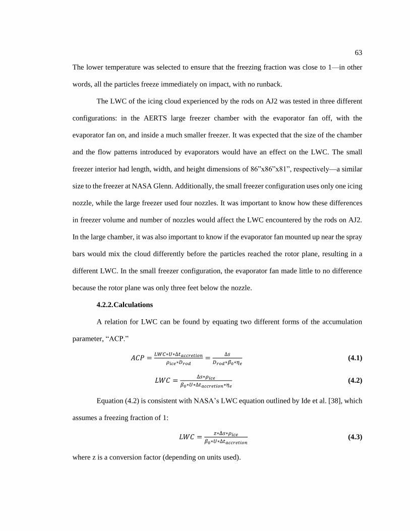
63
The lower temperature was selected to ensure that the freezing fraction was close to 1—in other
words, all the particles freeze immediately on impact, with no runback.
The LWC of the icing cloud experienced by the rods on AJ2 was tested in three different
configurations: in the AERTS large freezer chamber with the evaporator fan off, with the
evaporator fan on, and inside a much smaller freezer. It was expected that the size of the chamber
and the flow patterns introduced by evaporators would have an effect on the LWC. The small
freezer interior had length, width, and height dimensions of 86”x86”x81”, respectively—a similar
size to the freezer at NASA Glenn. Additionally, the small freezer configuration uses only one icing
nozzle, while the large freezer used four nozzles. It was important to know how these differences
in freezer volume and number of nozzles would affect the LWC encountered by the rods on AJ2.
In the large chamber, it was also important to know if the evaporator fan mounted up near the spray
bars would mix the cloud differently before the particles reached the rotor plane, resulting in a
different LWC. In the small freezer configuration, the evaporator fan made little to no difference
because the rotor plane was only three feet below the nozzle.
4.2.2. Calculations
A relation for LWC can be found by equating two different forms of the accumulation
parameter, “ACP.”
𝐴𝐶𝑃 =𝐿𝑊𝐶∗𝑈∗∆𝑡𝑎𝑐𝑐𝑟𝑒𝑡𝑖𝑜𝑛
𝜌𝑖𝑐𝑒∗𝐷𝑟𝑜𝑑=
∆𝑠
𝐷𝑟𝑜𝑑∗𝛽0∗𝜂𝑒 (4.1)
𝐿𝑊𝐶 =∆𝑠∗𝜌𝑖𝑐𝑒
𝛽0∗𝑈∗∆𝑡𝑎𝑐𝑐𝑟𝑒𝑡𝑖𝑜𝑛∗𝜂𝑒 (4.2)
Equation (4.2) is consistent with NASA’s LWC equation outlined by Ide et al. [38], which
assumes a freezing fraction of 1:
𝐿𝑊𝐶 =𝑧∗Δ𝑠∗𝜌𝑖𝑐𝑒
𝛽0∗𝑈∗∆𝑡𝑎𝑐𝑐𝑟𝑒𝑡𝑖𝑜𝑛 (4.3)
where z is a conversion factor (depending on units used).

64
To find the LWC, the freezing fraction and collection efficiency must be determined. The
MATLAB script used to calculate LWC in the Penn State icing lab was developed by Yiqiang Han
and Jose Palacios. It requires input parameters of the rod diameter, static temperature, impact
velocity, MVD, icing time, and measured ice thickness, which are known from the LWC
experiment. These values are summarized in Table 4.1.
Table 4.1: LWC Test Parameters for All Three LWC Configurations
Rod diam. 0.7938 cm
Rotor speed 1500 rpm
Airspeed 28.61 m/s
MVD 20 μm
Icing time 45 sec
Static temp. -20 ˚C
The code approximates the collection efficiency using the modified inertia parameter of the water
droplets, which is calculated using the airspeed and MVD. It then performs iterative heat transfer
calculations to converge on the freezing fraction.
4.2.3. Results
The results of the LWC tests are displayed in Figure 4.2.
Figure 4.2: Average LWC Values Obtained for Each Configuration

65
Based on the data collected, Figure 4.3 shows the approximate region in the FAR Appendix
C conditions [40] that was simulated on AJ2 during the preliminary impact ice adhesion tests. The
average LWC for each configuration was plotted on Figure 4.3 assuming an MVD of 20.
Figure 4.3: Approximate Region of FAR Appendix C Icing Conditions [40] Simulated by AJ2
Configurations in the Small Freezer and Large Freezer
In the large freezer configuration, the LWC varied by 10-15 percent; in the small freezer
the variation was approximately 5 percent. The large freezer configuration with the evaporator fan
on had approximately the same LWC as the small freezer configuration (~1 g/m3), but with the
evaporator fan off, the average LWC decreased significantly to 0.68 g/m3. It is suspected that the
evaporator fan created air currents inside the freezer that helped push the droplets down toward the
rotor plane and forced them to impact the rig and the walls. After test runs with the fan off, it was
noted that the air was very thick with shimmering droplets that had floated around and not landed
anywhere after leaving the nozzle. This never occurred with the fan on; all droplets had been forced

66
to impact either the rig or the walls and freeze. Another possible reason for the discrepancy is that
the evaporator fan currents may have moved droplets from the other three nozzles—not just the
one directly above the rig—over towards the rotor plane, resulting in a higher concentration of
water. Regardless of the reason, this difference was an important piece of information to know for
adhesion testing, and it explained why the large freezer defrost cycles were affecting the ice
accretion rate. It is therefore critical to maintain constant chamber fan conditions to ensure that the
LWC values do not grossly deviate from test to test.
4.3. Fixed-Speed Adhesion Testing
4.3.1. Procedure
All the fixed-speed and strain rate adhesion data presented in this thesis was collected in
the large AERTS freezer. Routine fixed-speed adhesion tests are performed almost identically to
adhesion tests on the large AERTS stand. First the user enters the coupon masses, test temperature,
and output file name into the LabVIEW VI. The user should monitor the coupon static temperatures
using the temperature plots from the on-blade thermistors, and ensure that the temperature remains
within ±1˚C of the desired test temperature throughout the entire experiment. Once the “Save Shed
Data” button is pressed, LabVIEW begins writing data points to the output text files. The strain
gauge plots will output a baseline voltage, labeled in Figure 4.4 as V0. After a few seconds, the user
will set the desired motor speed in the Drive Composer software and press the start button. The
motor will accelerate to the speed setpoint, where the second voltage value, V1, is taken. The speed
can be monitored at any given point in time using either the Hall sensor output on LabVIEW or in
the Drive Composer window itself. In Figure 4.4 the speed is labeled as 3100 rpm because that was
the rotational speed required to obtain the same droplet impact velocity as the large-scale AERTS
stand at 400 rpm. Fixed-speed adhesion tests on AJ2 were performed at 3100 rpm so the results
would be comparable to previous data.
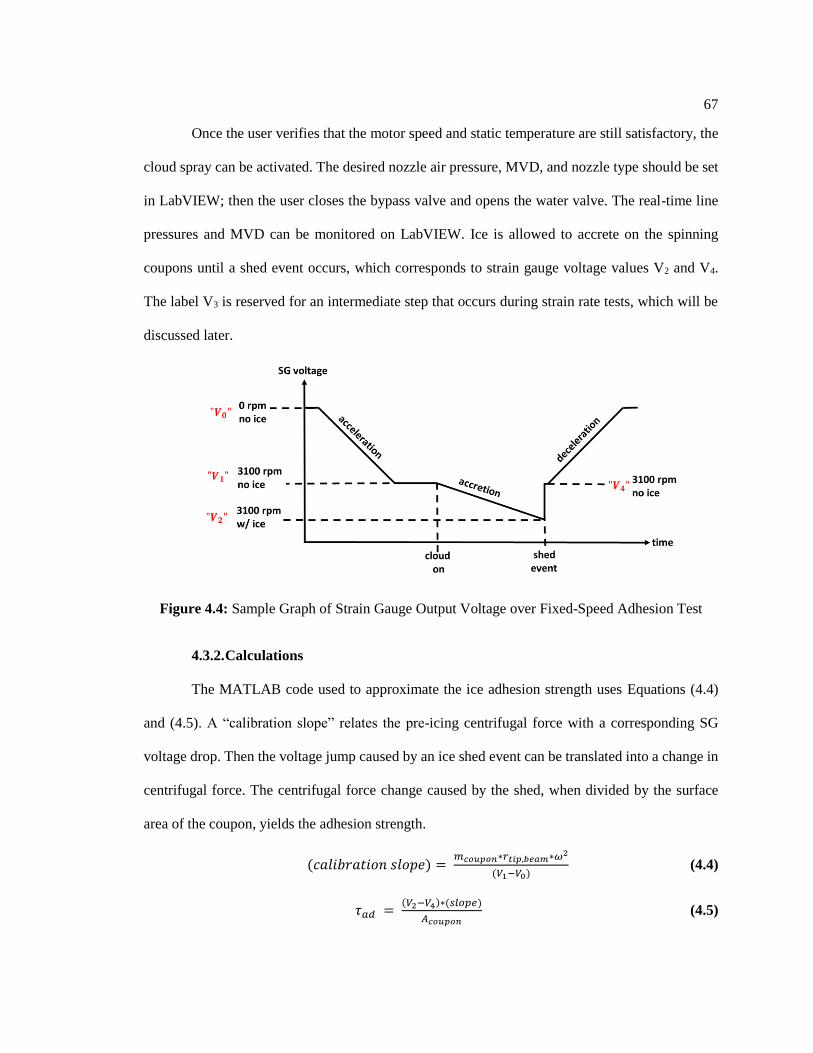
67
Once the user verifies that the motor speed and static temperature are still satisfactory, the
cloud spray can be activated. The desired nozzle air pressure, MVD, and nozzle type should be set
in LabVIEW; then the user closes the bypass valve and opens the water valve. The real-time line
pressures and MVD can be monitored on LabVIEW. Ice is allowed to accrete on the spinning
coupons until a shed event occurs, which corresponds to strain gauge voltage values V2 and V4.
The label V3 is reserved for an intermediate step that occurs during strain rate tests, which will be
discussed later.
Figure 4.4: Sample Graph of Strain Gauge Output Voltage over Fixed-Speed Adhesion Test
4.3.2. Calculations
The MATLAB code used to approximate the ice adhesion strength uses Equations (4.4)
and (4.5). A “calibration slope” relates the pre-icing centrifugal force with a corresponding SG
voltage drop. Then the voltage jump caused by an ice shed event can be translated into a change in
centrifugal force. The centrifugal force change caused by the shed, when divided by the surface
area of the coupon, yields the adhesion strength.
(𝑐𝑎𝑙𝑖𝑏𝑟𝑎𝑡𝑖𝑜𝑛 𝑠𝑙𝑜𝑝𝑒) = 𝑚𝑐𝑜𝑢𝑝𝑜𝑛∗𝑟𝑡𝑖𝑝,𝑏𝑒𝑎𝑚∗𝜔2
(𝑉1−𝑉0) (4.4)
𝜏𝑎𝑑 = (𝑉2−𝑉4)∗(𝑠𝑙𝑜𝑝𝑒)
𝐴𝑐𝑜𝑢𝑝𝑜𝑛 (4.5)

68
4.3.3. Results
4.3.3.1. Sample Photos
Fixed-speed adhesion tests were performed at -8˚C and -12˚C for comparison against
results from the large AERTS stand. In addition to adhesion strength data, sample photos were
taken to show the qualitative features of the accreted ice in different testing conditions.
Figure 4.5: Glaze Ice Accreted at -8˚C on a Laser-Ablated Coupon
Figure 4.6: Mixed/Rime Ice Accreted at -12˚C on 320-Grit Sample
Tests at -8˚C yielded glaze ice, which is characterized by water that flows before it freezes,
resulting in large horns and a transparent appearance. Reducing the temperature to -12 ˚C pushed
the environment further towards the rime regime. Rime ice is the type of ice used in LWC tests—

69
it generally conforms to the original coupon geometry. As shown in Figure 4.6, rime ice is milky
white due to the air bubbles that get trapped when the droplets freeze instantaneously. It should
also be noted that only ½” or less of ice typically accreted before shedding, due to high centrifugal
loads on the AJ2 rig. On the large AERTS stand, the ice sometimes grew over 1” thick before it
shed because of the low rotational speed.
According to the FAA online icing course for pilots [41], glaze ice tends to form above -
10˚C, mixed ice occurs between -10 and -15, and rime occurs lower than -15 degrees. However,
icing regime is also dependent on other parameters such as airspeed, LWC, and MVD, as
summarized in Figure 4.7:
Figure 4.7: Characteristics of Glaze and Rime Icing Regimes
With these differences in mind, the ice adhesion strength was evaluated on stainless steel
test coupons in both glaze and rime conditions, and with varying surface roughnesses.
4.3.3.2. Adhesion Data
The stainless-steel test coupons used for adhesion testing had a diameter of 1” and had been
polished with different polishing pads and compounds to achieve a range of surface roughness
values. The surface roughness values for all the tested surfaces are listed in Table 4.2.
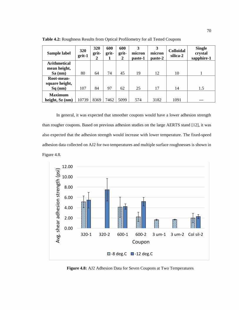
70
Table 4.2: Roughness Results from Optical Profilometry for all Tested Coupons
Sample label 320
grit-1
320
grit-
2
600
grit-
1
600
grit-
2
3
micron
paste-1
3
micron
paste-2
Colloidal
silica-2
Single
crystal
sapphire-1
Arithmetical
mean height,
Sa (nm) 80 64 74 45 19 12 10 1
Root-mean-
square height,
Sq (nm) 107 84 97 62 25 17 14 1.5
Maximum
height, Sz (nm) 10739 8369 7462 5099 574 3182 1091 ―
In general, it was expected that smoother coupons would have a lower adhesion strength
than rougher coupons. Based on previous adhesion studies on the large AERTS stand [12], it was
also expected that the adhesion strength would increase with lower temperature. The fixed-speed
adhesion data collected on AJ2 for two temperatures and multiple surface roughnesses is shown in
Figure 4.8.
Figure 4.8: AJ2 Adhesion Data for Seven Coupons at Two Temperatures
0.00
2.00
4.00
6.00
8.00
10.00
12.00
320-1 320-2 600-1 600-2 3 um-1 3 um-2 Col sil-2
Avg
. sh
ear
adh
esio
n s
tren
gth
(p
si)
Coupon
-8 deg.C -12 deg.C

71
Data that is missing in Figure 4.8 indicates that the coupon in question was sent out for re-
surfacing before testing could be performed at both temperatures. At -8˚C, there is a clear trend of
decreasing adhesion strength with decreasing surface roughness. At -12 ̊ C, the data does not appear
to follow this trend. This could indicate that the transition to the rime regime alters the behavior of
the ice with respect to the surface. It is also possible that previous testing at -8˚C changed the
surface morphology of the coupons before the -12 ˚C tests. Although stainless steel is significantly
harder than ice, consistent cycles of droplet impacts, freezing, expansion, and ripping off ice could
have degraded the original polished surface.
The data from AJ2 were compared to data from AERTS tests on the same coupons. The
results are shown in Figure 4.9 and Figure 4.10. The results are presented in order of decreasing
surface roughness. Note that the label “SS” refers to a stainless-steel surface, which applies to all
but the final coupon. The final coupon label “SCS” indicates a single-crystal sapphire surface.
Figure 4.9: -8°C Adhesion Strength Results for Large AERTS and AJ2 Rigs
0.00
2.00
4.00
6.00
8.00
10.00
12.00
14.00
16.00
18.00
20.00
22.00
SS-80nm SS-74nm SS-64nm SS-45nm SS-29nm SS-24nm SS-19nm SS-12nm SS-10nm SCS-1nm
Avg
. Sh
ear
Ad
hes
ion
Str
engt
h (
psi
)
Surface Roughness (Sa)
-8°C AERTS vs. AJ2
AERTS AJ2

72
Figure 4.10: -12°C Adhesion Strength Results for Large AERTS and AJ2 Rigs
The large AERTS stand consistently recorded higher adhesion strength values than the AJ2
stand. This may be because AERTS spins at a lower speed and therefore collects more ice before
the ice sheds. The higher ice thickness (up to 2”) effectively adds length to the bending beam,
increasing the CF-induced bending moment and the strain at the root of the beam. The assumption
that the ice is in pure shear is technically only true for an infinitesimally thin layer of ice—thick
ice is subject to a “peeling” moment that puts sections of the ice puck in tension or compression.
Therefore, the additional loading may make AERTS more prone to over-predict the adhesion
strength.
It is also interesting to note that, despite the fact that the single-crystal sapphire coupon
was 10 times smoother than the smoothest stainless-steel sample, its adhesion strength was equal
to or worse than the smooth stainless steel. The different material properties of the sapphire may
have caused it to behave differently than steel under high-speed droplet impact. A more-thorough
0.00
2.00
4.00
6.00
8.00
10.00
12.00
14.00
16.00
18.00
20.00
22.00
SS-80nm SS-74nm SS-64nm SS-45nm SS-29nm SS-24nm SS-19nm SS-12nm SS-10nm SCS-1nm
Avg
. Sh
ear
Ad
hes
ion
Str
engt
h (
psi
)
Surface Roughness (Sa)
-12°C AERTS vs. AJ2
AERTS AJ2

73
examination of the surface morphology and material properties would be needed further investigate
this hypothesis. Such effort is beyond the scope of this work.
Having obtained baseline adhesion-strength data at a fixed speed and variable temperature
and surface roughness, variable strain rate was tested next. The ability of AJ2 to perform tests like
the large AERTS stand had been verified; the next step was to examine the effects of variables that
AERTS could not test—namely, acceleration rate.

74
Chapter 5
Experimental Results of Strain Rate Adhesion Tests
The relationship between strain rate and shear adhesion strength observed in the AJ2
experiments in the current study followed a power function similar to the trends described in
literature [14, 17, 19]. Coupons of three different surface roughness values were tested. They
included two polished with a 320-grit polishing pad and one polished with a 600-grit polishing pad.
The surface roughness values obtained from the polishing process were quantified with optical
profilometry and are shown in Table 5.1.
Table 5.1: Surface Roughness Values of Strain-Rate-Tested Coupons
Coupon Sa (avg.,
nm)
Sq (RMS,
nm)
Sz (peak-peak,
nm)
320-1 80 107 10739
320-2 64 84 8369
600-1 74 97 7462
As the rotor spun at 1500 rpm, an icing cloud with 20-micron MVD was sprayed onto the
coupons for a set amount of time ranging between 30 seconds and 2 minutes. The chosen icing
time depended on the test temperature and surface roughness, since different ice thickness was
needed for shedding at varying temperatures and coupon surfaces.
After the elapsed time and before the ice could shed naturally at the accretion rpm, the
cloud was deactivated and the rotor speed was ramped up at a known acceleration rate. The
rotational speed at which the ice shed off, as well as the selected acceleration rate, dictated the
strain rate imposed on the ice. Values for strain rate and adhesion strength were obtained after
each test using the equations previously derived in Chapter 3. The motor acceleration rates tested
ranged from 1 rpm per second to 100 rpm per second.

75
Strain rate and adhesion strength data are plotted in Figure 5.1 using logarithmic axes. The
power regression function for each data series is also plotted. In Figure 5.1 A and B, the functions
for the smoother coupon had higher coefficients and higher powers than for the rougher coupon.
This occurred for both the rime and glaze condition (-16 and -8°C). This suggests that, for the range
of strain rates tested, smoother metallic surfaces react more strongly to increased strain rate than
slightly rougher surfaces.
In Figure 5.1 C and D, the effects of decreasing temperature can be observed. Glen [14]
found that for ice pucks under constant compressive stress, the temperature affected only the
coefficient of the function, not the power. However, Figure 5.1 C shows that for a given surface
roughness, decreasing temperature appears to increase both the 1/n power and the coefficient.
Unfortunately, the 74-nm sample was tested only at -12°C, so caution must be taken when directly
comparing that data series to the others. The lowest data points in the -12°C series were obtained
with an acceleration rate of 1 rpm per second. This extremely slow acceleration was not used for
subsequent testing, primarily because the tests runs at that acceleration were extremely time-
consuming and the slip ring would start to heat up beyond acceptable temperatures.

76
Figure 5.1: Strain Rate vs. Shear Adhesion Strength Data from AJ2 Tests. For reference, the top
left graph is (A), top right (B), bottom left (C), bottom right (D).
y = 140.11x0.2301
y = 1169.2x0.3927
1
10
100
5E-07 5E-06 5E-05
Shea
r A
dh
esio
n S
tren
gth
(p
si)
Acceleration Strain Rate at Failure (1/s)
-16 C, 80 nm
-16 C, 64 nm
y = 37.07x0.1031
y = 176.78x0.2277
1
10
100
5E-07 5E-06 5E-05
Shea
r A
dh
esio
n S
tren
gth
(p
si)
Acceleration Strain Rate at Failure (1/s)
-8 C, 80 nm
-8 C, 64 nm
y = 140.11x0.2301
y = 37.07x0.1031
y = 82.87x0.1535
1
10
100
5E-08 5E-07 5E-06 5E-05
Shea
r A
dh
esio
n S
tren
gth
(p
si)
Acceleration Strain Rate at Failure (1/s)
-8 C, 80 nm
-16 C, 80 nm
-12 C, 74 nm
y = 1169.2x0.3927
y = 176.78x0.2277
y = 82.87x0.1535
1
10
100
5E-08 5E-07 5E-06 5E-05
Shea
r A
dh
esio
n S
tren
gth
(p
si)
Acceleration Strain Rate at Failure (1/s)
-8 C, 64 nm
-16 C, 64 nm
-12 C, 74 nm
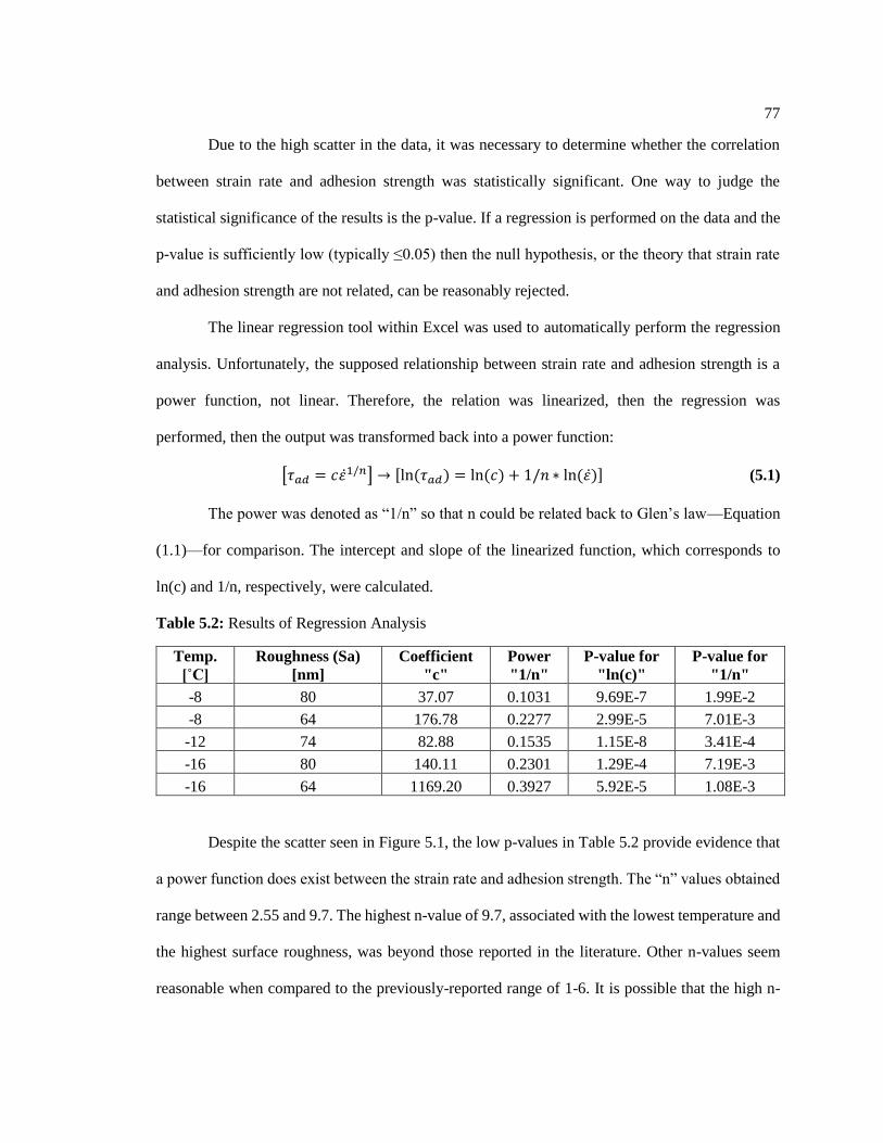
77
Due to the high scatter in the data, it was necessary to determine whether the correlation
between strain rate and adhesion strength was statistically significant. One way to judge the
statistical significance of the results is the p-value. If a regression is performed on the data and the
p-value is sufficiently low (typically ≤0.05) then the null hypothesis, or the theory that strain rate
and adhesion strength are not related, can be reasonably rejected.
The linear regression tool within Excel was used to automatically perform the regression
analysis. Unfortunately, the supposed relationship between strain rate and adhesion strength is a
power function, not linear. Therefore, the relation was linearized, then the regression was
performed, then the output was transformed back into a power function:
[𝜏𝑎𝑑 = 𝑐𝜀̇1/𝑛] → [ln(𝜏𝑎𝑑) = ln(𝑐) + 1/𝑛 ∗ ln(𝜀̇)] (5.1)
The power was denoted as “1/n” so that n could be related back to Glen’s law—Equation
(1.1)—for comparison. The intercept and slope of the linearized function, which corresponds to
ln(c) and 1/n, respectively, were calculated.
Table 5.2: Results of Regression Analysis
Temp.
[˚C]
Roughness (Sa)
[nm]
Coefficient
"c"
Power
"1/n"
P-value for
"ln(c)"
P-value for
"1/n"
-8 80 37.07 0.1031 9.69E-7 1.99E-2
-8 64 176.78 0.2277 2.99E-5 7.01E-3
-12 74 82.88 0.1535 1.15E-8 3.41E-4
-16 80 140.11 0.2301 1.29E-4 7.19E-3
-16 64 1169.20 0.3927 5.92E-5 1.08E-3
Despite the scatter seen in Figure 5.1, the low p-values in Table 5.2 provide evidence that
a power function does exist between the strain rate and adhesion strength. The “n” values obtained
range between 2.55 and 9.7. The highest n-value of 9.7, associated with the lowest temperature and
the highest surface roughness, was beyond those reported in the literature. Other n-values seem
reasonable when compared to the previously-reported range of 1-6. It is possible that the high n-

78
value could be related to the fact that previous studies did not use dynamically-accreted impact ice
in shear.
Since we acknowledge that the process of ice accretion itself imposes a strain rate on the
interface, it was necessary to use Equation (3.6) from Chapter 3 to calculate the strain rate values
associated with ice accretion. Ideally those values would be very small, because the goal was to
investigate strain rate effects in a controllable manner (i.e., with acceleration), and strain rate due
to ice growth is a side effect that is not possible to control with dynamically-grown ice.
The accretion strain rate was calculated for each test run. Over the entire population of data
for all temperatures and coupons, the average accretion strain rate was 5.64E-8 [/s] with a standard
deviation of 4.41E-8 [/s].
Figure 5.2: Accretion Strain Rate Range Superimposed on Acceleration Strain Rate Graph

79
For most of the runs (86%) the strain rate imposed by the ice accretion was less than 10
percent of the strain rate imposed by motor acceleration. However, at very low acceleration rates
of 1 rpm/s and 5 rpm/s, the strain rate at ice failure was very low and approached the accretion
strain rate range. In those cases, it is unclear whether the ice actually failed due to the acceleration,
or if it failed naturally under strain rates characteristic of the accretion phase of the test.

80
Chapter 6
Conclusions and Recommendations for Future Work
6.1. Conclusions
A small-scale ICAT-type ice adhesion test rig, dubbed “AJ2,” was successfully designed
and fabricated at Penn State. A NASA-grade icing nozzle was used to simulate a cloud of
supercooled droplets inside a walk-in freezer. Adhesion tests on AJ2 can be performed at rotor
speeds up to 5000 rpm, corresponding to a droplet impact speed of 180 kts, which is on the order
of actual in-flight impact speeds. The angular acceleration of the rotor can be controlled, allowing
the strain rate on the ice to be varied. Additionally, the entire system is controlled remotely, so
experimental data is not polluted by direct contact with the ice samples. After a shed event, the
adhesion strength of the ice is calculated using voltage measurements from strain gauges and the
known surface area of flat test coupons.
In the current study, the effect of strain rate (due to acceleration) on impact ice adhesion
strength was examined. Power functions were fit to the data by performing linear regression on the
natural log of the data points. The test coupon with lowest surface roughness appeared to have a
higher coefficient and power in its power function than the rougher samples. This same trend was
observed for lower environmental temperatures. The powers were compared to the “n” power from
Glen’s law [14] for the creep of polycrystalline ice under a compressive load. The n-values from
the current study range from 2.5 at the coldest temperature and smoothest sample, to 9.7 for the
warmest temperature and roughest sample. The fact that the coefficient “c” (related to the inverse
of Glen’s k-coefficient) increased with decreasing temperature is consistent with Glen’s
observations. Values of “n” in literature for lab-grown polycrystalline ice in compression tended to
range from about 2.5 to 3.5, making 9.7 seem large. However, Parameswaran [19] observed an n-
value of 5.8 for lab-grown polycrystalline ice in pure shear. Perhaps caution must be taken when
81
directly comparing current adhesion results from those in literature, because most previous strain
rate experiments were performed in compression instead of shear, and even those performed in
shear, like Parameswaran’s, did not use dynamically-accreted impact ice.
The strain rates obtained in this study ranged from ~5E-7 to ~5E-5 s-1. These are relatively
low strain rates compared to the ones reported in literature. In future testing, using higher
acceleration rates above 100 rpm per second would allow researchers to test higher strain rates on
the ice. It would be very interesting to explore the threshold at which strain rate becomes
independent of adhesion strength. A past study performed in compression [17] reported this strain
rate to be around 10-3 s-1. The threshold also likely changes with different metallic or polymer
surfaces, which should be explored. The three coupons tested in this study were all polished
stainless steel with similar surface roughness values. In the future, a wider range of surface
roughness values should be used, to verify that the strain rate-adhesion strength relationship
becomes more pronounced with smoother surfaces.
6.2. Future Work
Before the rig is installed at NASA, the current strain gauge setup will be replaced with
PCB piezoelectric strain sensors, mounted on the inner root of each beam. The new gauges measure
dynamic strain instead of static strain, so the voltage will hover around zero until a shed event
occurs. The decision to change the strain gauges was motivated by the need to frequently replace
the old strain gauge assembly. As shown in Figure 2.25, the marine epoxy would periodically fail
over many cycles of thermal expansion and centrifugal loading. Between preparing the beam
surface, applying the gauges, soldering all the wires, and waiting for epoxy to dry, the process of
replacing the current strain gauges took over 24 hours. The PCB strain sensors are sealed inside a
titanium housing, do not require marine epoxy, and can be easily removed and reused. Another
advantage to the PCB sensors is that they are pre-calibrated with a specified voltage-to-strain ratio.
Therefore, the voltage differential associated with a shed event can be easily used to find strain,

82
stress, and adhesion strength. It eliminates the need to use V0 and V1 to calibrate the gauges and
greatly simplifies calculations. One PCB sensor was applied to a test beam and used in a fixed-
speed adhesion test. Using the new sensor, the adhesion strength on a colloidal-silica polished
sample was measured to be 3.85±0.75 psi. For comparison, the adhesion strength measured on the
same coupon with the old strain gauges was 2.01±0.94 psi on AJ2 and 3.79±1.15 psi on the large
AERTS stand. These results show that the new PCB sensors are a viable replacement for the old
strain gauges, and will be much more convenient for NASA researchers to maintain.
The AJ2 test rig will be delivered in the spring of 2019 to NASA Glenn Research Center,
where it will be used for tests inside the Icing Research Tunnel. These experiments will be unique
because the ice will accrete in a forward-flight condition (as opposed to a hover condition), with
droplets impacting and freezing on the coupons at different angles. The results will be relevant to
rotorcraft icing. Once testing in the calibrated IRT icing cloud is complete, the rig will be installed
in a walk-in freezer in the RIMELab, where further strain rate testing can continue. In general, a
larger data pool with more temperatures, surface roughness values, and strain rates is desired to
validate the trends seen in the current study, and to expand the test envelope. This information will
be valuable for future ice adhesion modeling and ice protection system design efforts.

83
REFERENCES
[1] Leary, W. M., We Freeze to Please: A History of NASA’s Icing Research Tunnel and the
Quest for Flight Safety, Washington, DC: National Aeronautics and Space Administration, 2002,
https://history.nasa.gov/sp4226.pdf.
[2] “31 October 1994 - Eagle Flight 4184,” Cockpit Voice Recorder Database,
https://www.tailstrike.com/311094.htm.
[3] “12 February 2009 - Colgan Air 3407,” Cockpit Voice Recorder Database,
https://www.tailstrike.com/120209.htm.
[4] “2014 Annual Safety Review,” European Aviation Safety Agency, 2015.
[5] Eick, D., “Aircraft Icing Accidents,” National Transportation Safety Board, Washington,
D.C., February 2015. https://ral.ucar.edu/sites/default/files/public/events/2015/in-flight-icing-
users-technical-interchange-meeting-tim/docs/eick-ntsb-ncar-icing-presentation.pdf.
[6] DiPlacido, N., Soltis, J., and Palacios, J., “Enhancement of Ultrasonic De-Icing via Tone
Burst Excitation,” Journal of Aircraft, Vol. 53, No. 6, 2016, pp. 1821-1829.
[7] Wright, T., “Electro-mechanical Deicing,” Air & Space Magazine, The Smithsonian
Institution, March 2004.
[8] Whitfield, B., “How It Works: Bleed Air,” Flying Magazine, December 14, 2016.
[9] Werner, J.B., “The Development of an Advanced Anti-Icing/Deicing Capability for U. S.
Army Helicopters, Volume 1: Design Criteria and Technology Considerations,” Lockheed-
California Company, November 1975. https://apps.dtic.mil/dtic/tr/fulltext/u2/a019044.pdf.
[10] “About TKS Ice Protection Systems,” CAV Ice Protection,
https://www.caviceprotection.com/content/about-tks-ice-protection-systems.

84
[11] Kreeger, R., Vargas, M., Tran, A., Wang, Y., Palacios, J., and Hadley, K., “Multi-scale
Materials Design for Inflight Icing Mitigation,” NASA, 2016,
https://ntrs.nasa.gov/archive/nasa/casi.ntrs.nasa.gov/20160010295.pdf.
[12] Soltis, J., Palacios, J., Eden, T., and Wolfe, D., “Evaluation of Ice-Adhesion Strength on
Erosion-Resistant Materials,” AIAA Journal, Vol. 53, No. 7, 2015, pp. 1825-1835.
[13] Work, A., and Lian, Y., “A Critical Review of the Measurement of Ice Adhesion to Solid
Substrates,” Progress in Aerospace Sciences, Vol. 98, 2018, pp. 1–26.
[14] Glen, J.W., “The creep of polycrystalline ice,” Proceedings of the Royal Society of London,
Series A, Mathematical and Physical Sciences, Vol. 229, No. 1175, 1955.
[15] Goldsby, D.L., and Kohlstedt, D.L., “Superplastic deformation of ice: Experimental
observations,” Journal of Geophysical Research, Vol. 106, No. B6, 2001, pp. 11,017-11,030.
[16] Gold, L.W., “Process of Failure in Ice,” Canadian Geotechnical Journal, Vol. 7, No. 4,
1970, pp. 405-413.
[17] Cole, D.M., “Strain-Rate and Grain-Size Effects in Ice,” Journal of Glaciology, Vol. 33, No.
115, 1987.
[18] Hewitt, I., “Rheology of ice,” University of Oxford,
https://people.maths.ox.ac.uk/hewitt/slides/hewitt_karthaus_rheology.pdf.
[19] Parameswaran, V.R., “Adfreeze strength of model piles in ice,” Canadian Geotechnical
Journal, Vol. 18, 1981, pp. 8-16.
[20] Susoff, M., Siegmann K., Pfaffenroth, C., and Hirayama, M., “Evaluation of icephobic
coatings—Screening of different coatings and influence of roughness,” Applied Surface Science,
Vol. 282, 2013, pp. 870-879.
[21] Work, A.H., Gyekenyesi, A.L., Kreeger, R.E., Salem, J.A., Vargas, M.M., and Drabiak,
D.R., “The Adhesion Strength of Impact Ice Measured Using a Modified Lap Joint Test,” 2018
Atmospheric and Space Environments Conference, AIAA, Atlanta, GA, June 25-29, 2018.

85
[22] Smith, J.G., Jr., Wohl, C.J., Palacios, J.L., Connelly, B.D., “Design and Development of a
Laboratory-Scale Ice Adhesion Testing Device,” 41st Annual Meeting of The Adhesion Society,
San Diego, California, Feb. 25-Mar. 1, 2018.
[23] Fortin, G., Beisswenger, A., and Perron, J., “Centrifuge Adhesion Test to Evaluate Icephobic
Coatings,” AIAA Journal, 2010, DOI: 10.2514/6.2010-7837.
[24] Stallabrass, J.R., and Price, R.D., “On the Adhesion of Ice to Various Materials,” National
Research Laboratories, Division of Mechanical Engineering, Low Temperature Laboratory,
Report LR-350, 1962.
[25] Cowper, G. R., “The Shear Coefficient in Timoshenko’s Beam Theory,” Journal of Applied
Mechanics, Vol. 33, No. 2, 1966, pp. 335–340.
[26] “Strain Gage Installation Technical Data,” OMEGA Engineering Inc.,
https://www.omega.com/techref/pdf/STRAIN_GAGE_TECHNICAL_DATA.pdf.
[27] Bidwell, C., and Papadakis, M., “Collection Efficiency and Ice Accretion Characteristics of
Two Full-Scale and One ¼-Scale Business Jet Horizontal Tails,” NASA/TM—2005-213653,
June 2005.
[28] Haidar, A., and Palacios, J., “Effect of Number of Tracks and Balancing Masses on Passive
Balancing Performance,” 2018 AIAA/ASCE/AHS/ASC Structures, Structural Dynamics, and
Materials Conference, 8-12 January 2018, DOI: 10.2514/6.2018-2214.
[29] Thearle, E. L., “Dynamic Balancing Machine,” United States Patent No. US1876524A,
1932.
[30] “Measuring Strain with Strain Gauges,” National Instruments, 25 May 2016,
http://www.ni.com/white-paper/3642/en/.
[31] Steen, L., Ide, R., Van Zante, J., and Acosta, W., “NASA Glenn Icing Research Tunnel:
2014 and 2015 Cloud Calibration Procedures and Results,” NASA/TM—2015-218758, May
2015.

86
[32] Soeder, R., Sheldon, D., Ide, R., Spera, D., and Andracchio, C., “NASA Glenn Icing
Research Tunnel User Manual,” NASA/TM-2003-212004, September 2003.
[33] “GRC Containment Design Guide,” October 1995.
[34] McGinty, B., “Von Mises Stress,”
http://www.continuummechanics.org/vonmisesstress.html.
[35] “Aluminum 6061-T6,” Aerospace Specification Metals, Inc., MatWeb LLC.,
http://asm.matweb.com/search/SpecificMaterial.asp?bassnum=ma6061t6.
[36] Cengel, Y., and Cimbala, J., Fluid Mechanics: Fundamentals and Applications, 2nd Edition,
McGraw-Hill, 2010.
[37] “Stainless Steel Fasteners: A Systematic Approach to their Selection,” Specialty Steel
Industry of North America (SSINA), http://www.ssina.com/download_a_file/fasteners.pdf.
[38] Ide, R.F., and Oldenburg, J.R., “Icing Cloud Calibration of the NASA Glenn Icing Research
Tunnel,” NASA/TM-2001-210689, March 2001.
[39] Palacios, J., Brouwers, E., Han, Y., Smith, E., “Adverse Environment Rotor Test Stand
Calibration Procedures and Ice Shape Correlation,” American Helicopter Society 66th Annual
Forum, Phoenix, AZ, May 11-13, 2010.
[40] Jeck, R., “Icing Design Envelopes (14 CFR Parts 25 and 29, Appendix C),” Office of
Aviation Research, Federal Aviation Administration, DOT/FAA/AR-00/30, April 2002.
[41] “Structural Icing Type,” ALC-33: Inflight Icing, Federal Aviation Administration,
https://www.faasafety.gov/gslac/alc/course_content.aspx?cID=33&sID=152&preview=true.