Effects of small noise on the DMD/Koopman spectrum

Shervin Bagheri

Linné Flow Centre

Dept. Mechanics, KTH, Stockholm

Sig33, Sandhamn, Stockholm, Sweden

May, 29, 2013

Questions

1.  What are effects of noise on self-sustained oscillations?

2.  How sensitive are self-sustained oscillations to noise?

3.  Can we quantify the sensitivity?

2

•  Thermoacoustic oscillations

–  Feedback loop between acoustic field and unsteady heat release

–  White noise introduced by a loudspeaker

–  Measure pressure and heat release

Combustion Experiment

3 Jegadeesan & Sujith, Proc. Comb. Inst. 2013

•  Noise modifies limit cycle amplitude and period

Combustion Experiment

4 Jegadeesan & Sujith, Proc. Comb. Inst. 2013

Increasing noise level

Observations: Combustion

•  Observed “drift” of the phase of pressure oscillations

–  4 cycles: measuremenst in phase with harmonic signal

-  100 cycles: phase drifted 45 degrees

5 Lieuwen, J. Sound & Vibration. 2001

Phase Drift

•  Phase drift increases exponentially with time

6

Figure 7. Dependence of the mean-squared phase drift upon the number of cycles for three di!erent combustoroperating condition and k values of (a) 30, (b) 75, and (c) 150. In all three subplots, the data were obtained at a meaninlet velocity of 14)2 m/s (top curve), 14)5 m/s (middle curve), and 14)6 m/s (bottom curve).

essentially random disturbances imposed on the system by, for example, turbulent#uctuations. To address this question, we have considered what type of results would beexpected if the phase drift were due to random processes. It will be shown that the majorityof the ensemble averaged phase drift characteristics described in the prior section can becaptured by a random walk model.

The basic assumption behind the random walk model is that the phase drift at any cycle,q!, is equal to its value at the prior cycle, q

!!", plus a perturbation, M

!, i.e.

q!"q

!!"#M

!"!!

"#"M

". This perturbation could be due to, for example, turbulent

#uctuations in velocity or temperature. We also assume that there is an uncertainty in

900 T. C. LIEUWEN

Lieuwen, J. Sound & Vibration. 2001

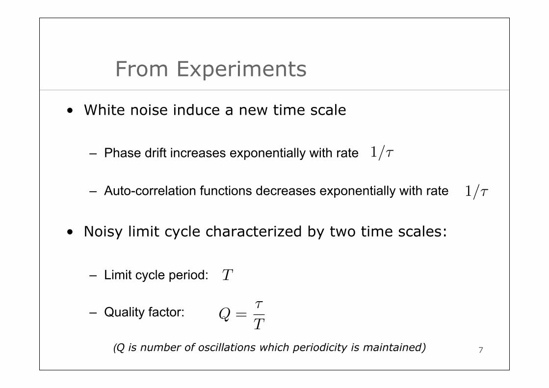
From Experiments

•  White noise induce a new time scale

–  Phase drift increases exponentially with rate

–  Auto-correlation functions decreases exponentially with rate

•  Noisy limit cycle characterized by two time scales:

–  Limit cycle period:

–  Quality factor:

(Q is number of oscillations which periodicity is maintained) 7

1/τ

1/τ

T

Q =τ

T

Koopman Operator

•  Time evolution of observables

–  governed by Koopman operator

–  approximated by Dynamic Mode Decomposition (DMD)

–  can be used to obtain time-correlation functions

Thus time scale should be present in the spectrum of the Koopman operator

8

τ

(Mezic, 2005, Rowley etal 2009)

(Schmid 2010)

Stochastic Navier-Stokes

•  Consider

–  state:

–  noise amplitude:

–  Gaussian white noise:

9

�ξ(t)ξ(t�)� = Qδ(t− t�)

∂u

∂t= f(u) +

√�ξ(t)

�

Evolution of Ensemble Average

•  Given an observable

–  Ensemble average of an observable at time t

: probability that a state will found in

–  Write ensemble average with linear evolution operators:

Koopman operator 10

g(u)

Eigenvalues of Koopman Operator

•  Koopman operator is linear

–  Eigenvalue decomposition:

–  At leading order the trace formula gives values for limit cycle:

11

(Gaspard, J. Stat. Phys. 2002)

m = 0,±1,±2, . . .

Ltg∗j (u) = λjg

∗j (u), j = 0, 1, 2, . . .

λm = imω − � |S|2T ω2m2 +O(�2)

Koopman eigenvalues for a noisy limit cycle

ω =2π

T

S = sensitivity

Globalmodes

2nd harmonicmodes

Globalmodes

2nd harmonicmodes

Mean !ow

Koopman Spectrum

–  Deterministic Koopman eigenvalues:

12

λm = imω

m = 0 m = 1 m = 2m = −2 m = −1

σ > 0

Bagheri, JFM 2013

2π/T

= im2π

T

Frequency

Gro

wth

rat

e

•  Koopman eigenvalues in the presence of noise

–  Non-stationary eigenvalues are damped! –  New time scale: (rate of phase diffusion) –  Proportional to (sensitivity)

Koopman Spectrum

τGlobalmodes

2nd harmonicmodes

Globalmodes

2nd harmonicmodes

Mean !ow

1/τ

m = 0 m = 1 m = 2m = −2 m = −1

m = 0,±1,±2, . . .λm = imω − � |S|2T ω2m2 +O(�2)

S

2π/T

Gro

wth

rat

e

Frequency

DMD of Noisy System: Helium Jet

•  DMD (often) approximates Koopman eigenvalues

•  Input: Sequence of snapshots (from experiments)

14 Schmid, Li, Juniper & Pust, TCFD, 2011

•  Output: DMD modes (coherent structures)

DMD of Noisy System: Helium Jet

15 Schmid, Li, Juniper & Pust, TCFD, 2011

•  Output: DMD values (growth rate and frequency)

•  Parabolas are due to the presence weak noise

•  DMD spectrum reveals two time scales

DMD of Noisy System: Helium Jet

16

(frequency)

(gro

wth

rate

)

1/τ2π/T

Sensitivity

•  How sensitive is a limit cycle to noise?

•  Large high rate of phase diffusion

•  What is the explicit expression for ?

17

λm = imω − � |S|2T ω2m2 +O(�2)

|S|

S

Stochastic Navier-Stokes

•  The stochastic system

can in limit of be written as

–  where is an “adjoint variable” –  noiseless system –  system with noise

18

∂u

∂t= f(u) +

√�ξ(t)

p = [−∇f(u)]T p

� → 0

p(t) ∈ Rn

dim = n

dim = 2n

Onsager & Machlup, Phys. Rev. 1953

Hamiltonian System

•  Hamiltonian:

–  Hamilton equations:

–  “Energy” conserved along trajectories (constant of motion)

–  “Energy” is measure of deviation of noisy trajectory from its deterministic prediction

19 Onsager & Machlup, Phys. Rev. 1953

dH

dt= 0 → H(u,p) = E

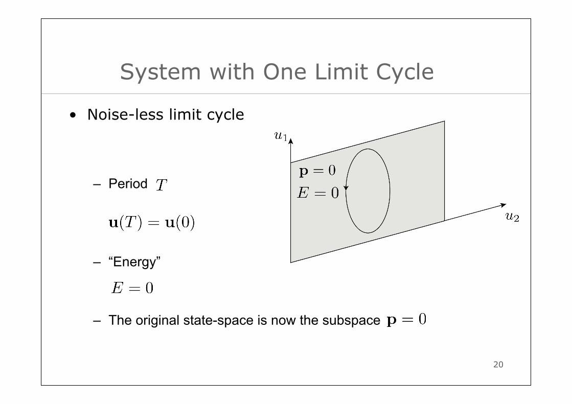
System with One Limit Cycle

•  Noise-less limit cycle

–  Period

–  “Energy”

–  The original state-space is now the subspace

20

•  Noisy limit cycle

of period

•  “Energy”

–  Dimension of original state space is doubled to accommodate for limit cycles of perturbed period

System with Noisy Limit Cycle

21

Sensitivity

•  Consider “Energy”

•  How does a small perturbation of “energy” affect the time period?

–  define sensitivity as

–  large a small perturbation of “energy”, gives large deviation from deterministic time period 22 ∂ET

E = �/τ

δT =

�∂T

∂E

�δE = SδE

Linearized System

•  Small we may linearize system

Write solution as

Floquet expansion

23

δT

δu = A(u) + 2Qδp

δp = −AT (u)δp

δu(T ) = MT δu(0) +NT δp(0)

δp(T ) = (M−1T )T δp(0)

MT =n�

k=1

φkΛkψTk

Sensitivity

•  One obtains the expression

if system is non-normal then

and

24

∂T

∂E= −ψT

1 δu(T )

ψT1 φ1

ψT1 φ1 � 1

∂T

∂E� 1S =

Sensitivity

•  One obtains the expression

is obtained by solving linearized equations with initial conditions:

25

∂T

∂E= −ψT

1 δu(T )

ψT1 φ1

δu(T ) = NTψ1

δu(0) = 0 δp(0) = ψ1

(Gaspard, J. Stat. Phys. 2002)

Conclusions

•  Sensitivity –  Noisy limit cycle may deviate from deterministic cycle if

system is highly non-normal

•  Quality factor can be read of the DMD spectrum –  Look into DMD literature: you observe parabolic

branches!

–  Important for control purposes

–  Determine whether randomness is due external noise or some intrinsic dynamics

26