Effects of Residual Moisture and Zero Conditioning Time … and Residual...Effects of Residual...

Effects of Residual Moisture and Zero Conditioning Time on Maximum Theoretical Specific Gravity

John P. Zaniewski, Ph.D.

John Crane

Asphalt Technology Program

Department of Civil and Environmental Engineering

Morgantown, West Virginia

3/4/2013

ii

NOTICE

The contents of this report reflect the views of the authors who are responsible for the

facts and the accuracy of the data presented herein. The contents do not necessarily reflect

the official views or policies of the State or the Federal Highway Administration. This report

does not constitute a standard, specification, or regulation. Trade or manufacturer names

which may appear herein are cited only because they are considered essential to the

objectives of this report. The United States Government and the State of West Virginia do

not endorse products or manufacturers. This report is prepared for the West Virginia

Department of Transportation, Division of Highways, in cooperation with the US Department

of Transportation, Federal Highway Administration.

iii

Technical Report Documentation Page

1. Report No. 2. Government

Association No.

3. Recipient's catalog No.

4. Title and Subtitle

Effects of Residual Moisture and Zero

Conditioning Time on Maximum Theoretical

Specific Gravity

5. Report Date December, 2012

6. Performing Organization Code

7. Author(s)

John P. Zaniewski, John E. Crane 8. Performing Organization Report No.

9. Performing Organization Name and Address

Asphalt Technology Program

West Virginia University

P.O. Box 6103

Morgantown, WV 26506-6103

10. Work Unit No. (TRAIS)

11. Contract or Grant No.

12. Sponsoring Agency Name and Address

West Virginia Division of Highways

1900 Washington St. East

Charleston, WV 25305

13. Type of Report and Period Covered

14. Sponsoring Agency Code

15. Supplementary Notes

Performed in Cooperation with the U.S. Department of Transportation - Federal Highway

Administration

16. Abstract

A critical issue in determining theoretical maximum specific gravity (Gmm) for Hot

Mix Asphalt (HMA) mixtures appears for high absorption aggregates. High absorption

aggregates, like slag, can greatly affect the Gmm values. The dry-back procedure for

measuring Gmm may not produce reliable results. Gmm results from lab prepared mixes were

observed to be different from plant prepared mixes. Two hypotheses were identified that may

cause this effect, residual moisture and conditioning time. To test the effects of residual

moisture samples of slag aggregate were saturated with water for a period of time then heated

allowing some of the water to evaporate and then mixed with other aggregates and binder.

Samples were also produced and tested without having the two hour conditioning time.

Findings indicated that a third of the residual moisture samples were significantly different

from the control values, with seventy percent of those samples containing high slag contents.

The conditioning time results showed that the lack of a conditioning period was significantly

different than the controlled two hour conditioning at a 95% confidence level.

A related issue is a vacuum method for measuring Gmm has been developed and is in

use by some contractors. The experimental design for this research compared the results of

the standard test method to the vacuum method. There is a small, but consistent difference

between the standard and vacuum methods.

17. Key Words

Slag, Maximum theoretical specific gravity,

HMAC Vacuum method

18. Distribution Statement

19. Security Classif. (of this

report)

Unclassified

20. Security Classif. (of

this page)

Unclassified

21. No. Of Pages 73

22. Price

Form DOT F 1700.7 (8-72) Reproduction of completed page authorized

iv

TABLE OF CONTENTS

1.1 Background ........................................................................................................................ 1

1.2 Problem Statement ............................................................................................................. 1

1.3 Objective ............................................................................................................................ 2

1.4 Organization of Report ...................................................................................................... 2

2.1 Introduction ....................................................................................................................... 3

2.2 Slag in HMAC ................................................................................................................... 3

2.2.2 Different Types of Slag ......................................................................................... 4

2.2.3 Benefits of ACBFS ............................................................................................... 4

2.2.4 Drawbacks of ACBFS ........................................................................................... 5

2.3 Test Methods ..................................................................................................................... 5

2.3.1 CoreLok ................................................................................................................ 5

2.3.2 Rice Method and Additional Dry-Back Procedures ............................................. 8

2.4 Gmm investigations Using the CoreLok ............................................................................ 10

2.4.1 Florida DOT ........................................................................................................ 10

2.4.2 University of Cincinnati ...................................................................................... 12

3.1 Introduction ..................................................................................................................... 15

3.2 Experimental Design ....................................................................................................... 15

3.3 Material ............................................................................................................................ 16

3.3.1 Asphalt Cement ................................................................................................... 16

3.3.2 Aggregate Properties ........................................................................................... 16

3.3.3 Aggregate Preparation ......................................................................................... 17

3.4 Mix Design ...................................................................................................................... 17

3.4.1 Aggregate Blends ................................................................................................ 18

3.5 Sample Creation .............................................................................................................. 19

3.5.1 Additional Procedures for Water Addition ......................................................... 21

3.5.1 Additional Procedures for Zero Conditioning Time ........................................... 23

3.6 Sample Testing ................................................................................................................ 23

3.6.1 Test Methods ....................................................................................................... 24

4.1 Introduction ..................................................................................................................... 25

4.2 Results ............................................................................................................................. 26

4.2.1 Gmm Analysis of Test Methods ........................................................................... 27

v

4.2.2 Analysis of Conditioning Time ........................................................................... 31

4.2.3 Gse Analysis ......................................................................................................... 35

4.3 Comparison to Previous Research ................................................................................... 40

5.1 Conclusions ..................................................................................................................... 44

5.2 Recommendations for Further Study ............................................................................... 45

References ................................................................................................................................ 48

Appendix – Data Sheets ........................................................................................................... 49

List of Tables

Table 1– FDOT t-test Results for Gmm Test Data for the CoreLok and FM 1-T 209 ....... 12

Table 2 - Comparison Data for AASHTO T-209 and CoreLok (Rajagopal and Crago

2007) ..................................................................................................................... 14

Table 3 - Experimental Factors/Levels ............................................................................. 15

Table 4 - Data Table ......................................................................................................... 16

Table 5 - Aggregate Properties ......................................................................................... 17

Table 6 – Aggregate Gradations ....................................................................................... 17

Table 7 - Combined Mixture Gradations & Properties ..................................................... 19

Table 8–Example Aggregate Weigh-out Table ................................................................ 21

Table 9 - Experimental Factors and Levels ...................................................................... 25

Table 10 - Description of Acronyms ................................................................................ 25

Table 11 - Gmm Test Results ............................................................................................. 26

Table 12 - Gmm Means and Standard Deviations .............................................................. 26

Table 13 - t-test comparisons of test methods .................................................................. 28

Table 14 - Results of Regression Analysis for Rice versus CoreLok ............................... 30

Table 15 - Gse Data Sheet.................................................................................................. 36

Table 16 - Gse Means and Standard Deviations ................................................................ 36

Table 17 - Slag Content Analysis Using Gse ..................................................................... 37

Table 18 - Gse Comparison for Additional Binder ............................................................ 39

Table 19 – Gmm Moisture Addition t-test Table ................................................................ 42

Table 20 - Regression analysis on Rajagopal and Crago Study ....................................... 43

Table 21 - Summary of Analytical Tests .......................................................................... 46

Table 22 - LD DATA ........................................................................................................ 49

vi

Table 23 - MD DATA....................................................................................................... 50

Table 24 - HD DATA ....................................................................................................... 51

Table 25 - LDM DATA .................................................................................................... 52

Table 26 - MDM DATA ................................................................................................... 53

Table 27 - HDM DATA .................................................................................................... 54

Table 28 - LZ DATA ........................................................................................................ 55

Table 29 - MZ DATA ....................................................................................................... 56

Table 30 - HZ DATA ........................................................................................................ 57

Table 31 - LZM DATA..................................................................................................... 58

Table 32 - MZM DATA ................................................................................................... 59

Table 33 - HZM DATA .................................................................................................... 60

Table 34 - LP DATA ........................................................................................................ 61

Table 35 - MP DATA ....................................................................................................... 62

Table 36 - HP DATA ........................................................................................................ 63

Table 37 - LPM DATA ..................................................................................................... 64

Table 38 - MPM DATA .................................................................................................... 65

Table 39 - HPM DATA .................................................................................................... 66

List of Figures

Figure 1 - The CoreLok Vacuum Machine with the Agg. Plus Device .............................. 6

Figure 2 - CoreLok Procedure Step A: 1500 g placed in the channel bag. ......................... 6

Figure 3 - CoreLok Procedure Step B: Channel bag placed inside larger bag. ................. 7

Figure 4 - CoreLok Procedure Step C: Both bags and sample are placed in the CoreLok,

the lid is closed. After the vacuum and sealing processes are completed the bags

can be removed. ...................................................................................................... 7

Figure 5 - Data Chart for CoreLok Gmm Test ..................................................................... 9

Figure 6- Test set up for FDOT test method FM 1-T209 ................................................. 11

Figure 7 - Combined Mixture Gradations ......................................................................... 20

Figure 8 - Drying Rack ..................................................................................................... 24

Figure 9 - Line of Equality Chart for Rice versus CoreLok Gmm Results. ........................ 29

Figure 10 - Line of Equality Chart for Dry Back versus Rice Gmm Results. .................... 32

Figure 11 - Adjusted Line of Equality Chart for Dry Back versus Rice Gmm Results ...... 33

vii

Figure 12 - Line of Equality Chart for Dry Back versus CoreLok Gmm Results. ............. 33

Figure 13 - Conditioning Time Means.............................................................................. 34

Figure 14 - Gse Means ....................................................................................................... 37

Figure 15 - Gse Test Data versus Slag Content ................................................................. 38

Figure 16 - Line of Equality for Dry vs. Moist sample comparison ................................. 41

Figure 17 - Moisture Addition Line of Regression for Zero conditioned samples ........... 41

Figure 18 - Line of Equality on Rajagopal and Crago study ............................................ 43

1

Chapter 1 Introduction

1.1 Background

In order to correctly evaluate asphalt concrete’s volumetric properties the

theoretical maximum specific gravity (Gmm) must be accurately measured. This has

proven to be a problem when absorptive aggregates are used in a mixture. The dry-back

procedure has been implemented for years in attempt to correct this issue; however this

procedure is prone to errors. In more recent years a new device, the CoreLok, has been

released as an alternative method for measuring specific gravity of asphalt mixes.

One of the significant problems with the use of certain aggregates is their

absorptive properties. Once a sample of asphalt is mixed, the longer it conditions the

more asphalt is absorbed into the aggregates until the voids are saturated with asphalt.

This absorption greatly changes the Gmm value of the sample. This is then reflected in the

values for air voids and makes it more difficult for a contractor to achieve their correct

densities in the field while constructing a new pavement.

The need for improving specific gravity measurements is not unique to West

Virginia. The FHWA (2010) reviewed methods for determining specific gravity and the

associated impact on volumetric analysis of asphalt mixes. With respect to Gmm the

FHWA report states:

The current standard test methods for determination of Gmm for HMA mixtures containing aggregate with low absorption are satisfactory. However, the multilaboratory precision estimate for mixtures containing moderately to highly absorptive aggregate is so large that it is not valid to distinguish air voids results for split specimens conducted in two laboratories that differ by as much as 2.0 percent. Clearly, further work needs to be conducted to improve the reproducibility of the Gmm

determination for such aggregate. Another important objective for further research should be to reduce the time to complete the test for mixes containing absorptive aggregate.

1.2 Problem Statement

The material issue evaluated in the research is from an asphalt plant in the

southern part of West Virginia. West Virginia Paving, Dunbar, WV, has been having

2

issues with theoretical maximum specific gravity test results between laboratory

produced samples and samples taken from plant production. Plant produced samples

have lower Gmm values compared to those created in the laboratory for mix design. Two

main questions arose from discussions about this problem. Is there a small amount of

water still inside the absorptive material after it exits the asphalt plant? In this case the

water may evaporate out of the stone leaving small micro punctures in the asphalt coating.

Second, plant samples are pulled straight from the plant and tested; is there sufficient

time between mixing and testing to allow the asphalt to absorb into the voids of the slag?

In addition, a vacuum based procedure for measuring asphalt mix specific gravity

has been developed and is being used by some contractors. This method uses the

CoreLok system developed by Instrotek, Inc. The WVDOH has limited experience with

the CoreLok method. To gain experience with this test method, samples were evaluated

with the conventional (Rice) method, the CoreLok method and the dry-back process.

1.3 Objective

The objectives for this research were all observed to aid in determining a quality

answer for the theoretical maximum specific gravity. The three objectives are as

followed:

Is the Dry Back procedure necessary?

Can the CoreLok replace the original Rice Test (AASHTO’s T209)?

Is there a difference between the plant and laboratory processes?

Null hypotheses were used to distinguish if there was any difference between the test

methods and between the different sample variations described above.

1.4 Organization of Report

This report is organized into five chapters. Following the introduction, Chapter 2

contains background on the use of slag in hot mix asphalt pavements, brief history on the

T209 and CoreLok test methods, and finally summaries of research conducted with the

CoreLok. Chapter 3 discusses the research methodologies and test procedures that were

used in the laboratory to conduct the research. Chapter 4 contains the analysis of the

results from the laboratory findings. Finally in Chapter 5 conclusions and

recommendations are presented. The Appendix includes the test results for each mixture.

3

Chapter 2 Literature Review

2.1 Introduction

With the great quantities of waste products created each year there is a strong

push to find better uses for them. The transportation sector has been a great recipient of

these materials. Currently the Federal Highway Administration (FHWA) allows many

different kinds of by-products to be used in the construction of asphalt pavements; the list

below illustrates the wide span of materials.

Blast Furnace Slag

Coal Bottom Ash

Coal Boiler Slag

Foundry Sand

Mineral Processing Wastes

Municipal Solid Waste Combustor Ash

Nonferrous Slags

Reclaimed Asphalt Pavement

Roofing Shingle Scrap

Scrap Tires

Steel Slag

Waste Glass

While there are many allowable types of materials this research evaluated the use

of Blast Furnace Slag, therefore the remaining materials will not be mentioned further in

this report.

2.2 Slag in HMAC

Blast Furnace slag has become an important resource in many states for the use in

road construction and rehabilitation. At least 17 states have adopted the use of blast

furnace slag; several are located in the eastern United States. According to the US

Geological Survey in 2006 nearly 41.3% of air-cooled blast furnace slag was used for

road bases and surfaces, another 13.3% was used for asphaltic concrete (Van Oss, 2007).

Slag is a co-product of the production of iron and steel, along with other metals.

For the production of iron and steel, iron ore, scrap iron and steel, fluxes (limestone

and/or dolomite), and coke are placed in the blast furnace. The coke is then combusted to

reduce the iron ore to a molten state. The slag which primarily consists of silicates,

alumina-silicates, and calcium-alumina-silicates is less dense then iron therefore it floats

on the molten iron and can be separated from the iron product and removed as a co-

product. Although slag is less dense than iron slag’s density greatly depends on the

4

residual iron content in the slag. Typical specific gravities range from 2.0 to 2.5 for air

cooled slag (FHWA, 1997).

2.2.2 Different Types of Slag

Once the slag is formed in the blast furnace there are multiple ways to separate

the slag, which creates different products. The main methods are Air-Cooling, Expanded

or Formed, and Pelletized.

Air-cooled blast furnace slag (ACBFS) forms from the cooling of liquid slag that

is poured into large beds and is allowed to cool slowly under normal conditions. This

slow cooling allows the slag to form a hard crystalline structure. After the slag cools it is

crushed into usable sized aggregates.

Expanded slag is cooled with the use of water, steam, or air. This process allows

for an accelerated cooling which increases the size of the crystalline structure, leaving a

lightweight product. Expanded slag has a much higher porosity and lower specific

gravities if compared to air cooled slag.

Pelletized slag is formed when molten slag is quenched with water or air in a

spinning drum. The process forms pellets which can be controlled by the speed of the

quenching process. If the slag is rapidly cooled, less crystallization will occur and the

slag will have a glassy appearance (FHWA, 1997).

Air-cooled blast furnace slag will be discussed from this point on since it was

used for this experiment.

2.2.3 Benefits of ACBFS

The main benefits from the use of slag are some of its physical and mechanical

properties. ACBFS is angular with a roughly cubical shape. ACBFS also has good

frictional resistance, stripping resistance, and high stability. Slags high stability is due to

its high internal angle of friction, which is 40 to 45 degrees. The rough, porous, angular

surface and hardness (5 to 6) of slag all help contribute to a high frictional resistance. The

slag used in West Virginia has been approved as a skid resistant aggregate suitable for

use in wearing layers. Slag also has high polished stone values and an affinity to asphalt,

not water, and therefore, slag has high stripping resistance (FHWA, 1997).

5

2.2.4 Drawbacks of ACBFS

The two main flaws with the use of slag is its high absorption from its porous

surface, and the high variability in the material. The FHWA states that since there is

variation in the production process of iron that variability continues into the slag,

resulting in inconsistent results for gradations, specific gravities, absorptions, and

angularity. This lack of consistency contributes to HMAC performance problems, like

flushing, raveling, and high fines. Flushing is related to high binder content and raveling

is related to low binder content which could be from the inconsistency in the absorption

of ACBFS. Absorption is the other main drawback with slag. A high absorption requires

more asphalt to be added to the mixture, which adds cost to the mixture. The FHWA

says that this cost is usually offset by the high yield from using a slag mixture. The high

yield is due to the lower density of the slag, therefore more volume for the same amount

of weight (FHWA, 1997).

2.3 Test Methods

2.3.1 CoreLok

The CoreLok was developed by InstroTek Inc. located in Raleigh, North Carolina

and was released in the late 1990’s. InstroTek developed this vacuum sealing device to

address the limitations of the previous test methods. The CoreLok is not only used for

testing specific gravities for asphalt samples, it can test a wide variety of samples. This

includes apparent specific gravity, absorption, and bulk specific gravity of aggregates

using the AggPlus system. The CoreLok can also test for porosity of compacted asphalt

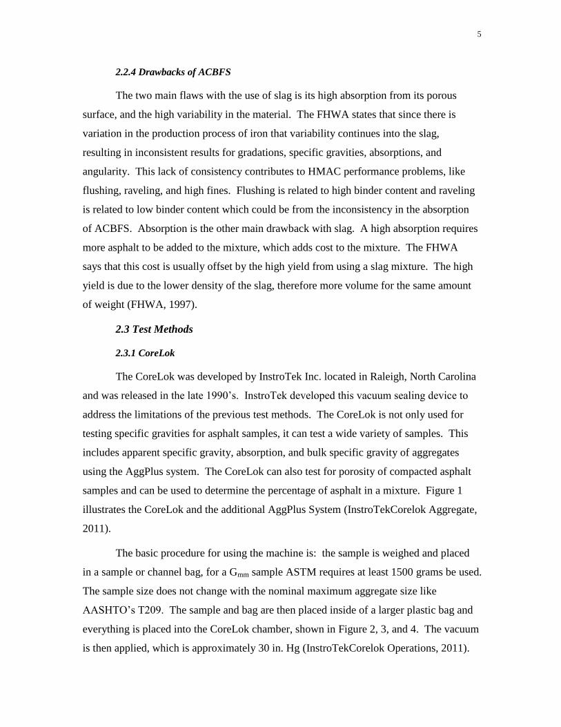
samples and can be used to determine the percentage of asphalt in a mixture. Figure 1

illustrates the CoreLok and the additional AggPlus System (InstroTekCorelok Aggregate,

2011).

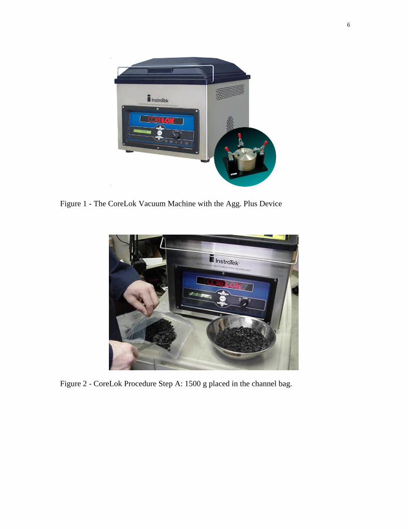
The basic procedure for using the machine is: the sample is weighed and placed

in a sample or channel bag, for a Gmm sample ASTM requires at least 1500 grams be used.

The sample size does not change with the nominal maximum aggregate size like

AASHTO’s T209. The sample and bag are then placed inside of a larger plastic bag and

everything is placed into the CoreLok chamber, shown in Figure 2, 3, and 4. The vacuum

is then applied, which is approximately 30 in. Hg (InstroTekCorelok Operations, 2011).

6

Figure 1 - The CoreLok Vacuum Machine with the Agg. Plus Device

Figure 2 - CoreLok Procedure Step A: 1500 g placed in the channel bag.

7

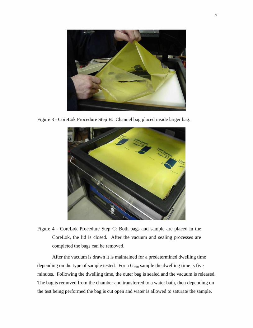
Figure 3 - CoreLok Procedure Step B: Channel bag placed inside larger bag.

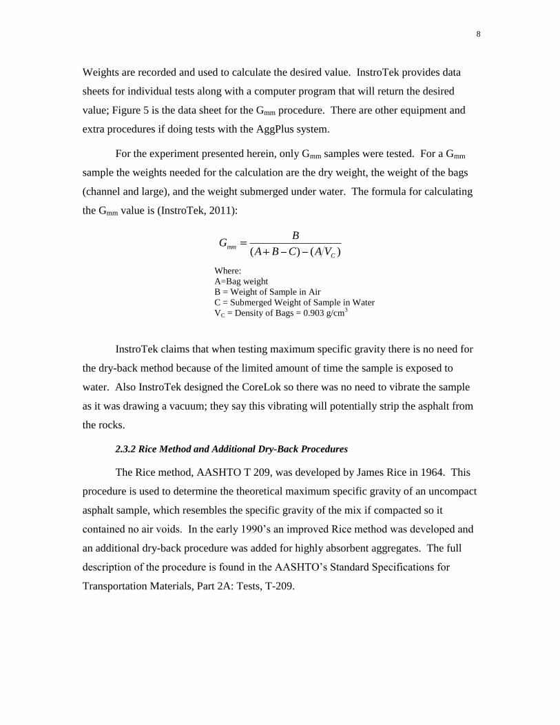
Figure 4 - CoreLok Procedure Step C: Both bags and sample are placed in the

CoreLok, the lid is closed. After the vacuum and sealing processes are

completed the bags can be removed.

After the vacuum is drawn it is maintained for a predetermined dwelling time

depending on the type of sample tested. For a Gmm sample the dwelling time is five

minutes. Following the dwelling time, the outer bag is sealed and the vacuum is released.

The bag is removed from the chamber and transferred to a water bath, then depending on

the test being performed the bag is cut open and water is allowed to saturate the sample.

8

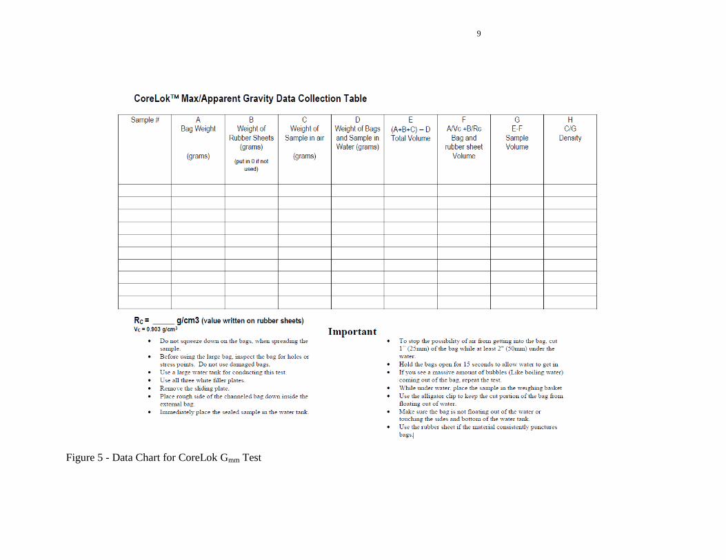
Weights are recorded and used to calculate the desired value. InstroTek provides data

sheets for individual tests along with a computer program that will return the desired

value; Figure 5 is the data sheet for the Gmm procedure. There are other equipment and

extra procedures if doing tests with the AggPlus system.

For the experiment presented herein, only Gmm samples were tested. For a Gmm

sample the weights needed for the calculation are the dry weight, the weight of the bags

(channel and large), and the weight submerged under water. The formula for calculating

the Gmm value is (InstroTek, 2011):

)()( C

mmVACBA

BG

Where:

A=Bag weight

B = Weight of Sample in Air

C = Submerged Weight of Sample in Water

VC = Density of Bags = 0.903 g/cm3

InstroTek claims that when testing maximum specific gravity there is no need for

the dry-back method because of the limited amount of time the sample is exposed to

water. Also InstroTek designed the CoreLok so there was no need to vibrate the sample

as it was drawing a vacuum; they say this vibrating will potentially strip the asphalt from

the rocks.

2.3.2 Rice Method and Additional Dry-Back Procedures

The Rice method, AASHTO T 209, was developed by James Rice in 1964. This

procedure is used to determine the theoretical maximum specific gravity of an uncompact

asphalt sample, which resembles the specific gravity of the mix if compacted so it

contained no air voids. In the early 1990’s an improved Rice method was developed and

an additional dry-back procedure was added for highly absorbent aggregates. The full

description of the procedure is found in the AASHTO’s Standard Specifications for

Transportation Materials, Part 2A: Tests, T-209.

9

Figure 5 - Data Chart for CoreLok Gmm Test

10

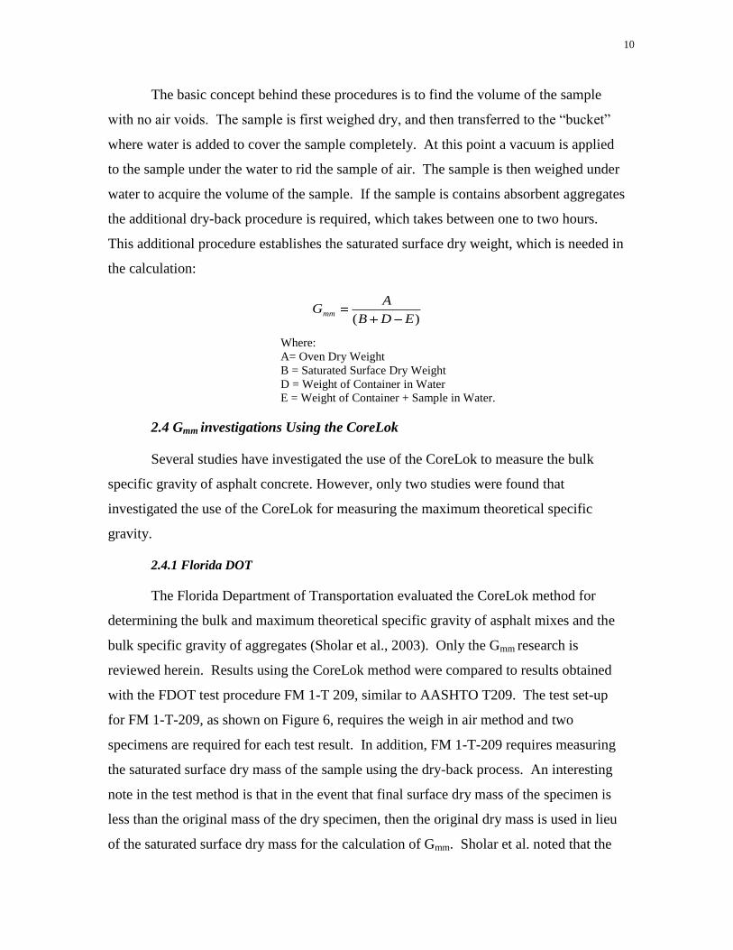
The basic concept behind these procedures is to find the volume of the sample

with no air voids. The sample is first weighed dry, and then transferred to the “bucket”

where water is added to cover the sample completely. At this point a vacuum is applied

to the sample under the water to rid the sample of air. The sample is then weighed under

water to acquire the volume of the sample. If the sample is contains absorbent aggregates

the additional dry-back procedure is required, which takes between one to two hours.

This additional procedure establishes the saturated surface dry weight, which is needed in

the calculation:

)( EDB

AGmm

Where:

A= Oven Dry Weight

B = Saturated Surface Dry Weight

D = Weight of Container in Water

E = Weight of Container + Sample in Water.

2.4 Gmm investigations Using the CoreLok

Several studies have investigated the use of the CoreLok to measure the bulk

specific gravity of asphalt concrete. However, only two studies were found that

investigated the use of the CoreLok for measuring the maximum theoretical specific

gravity.

2.4.1 Florida DOT

The Florida Department of Transportation evaluated the CoreLok method for

determining the bulk and maximum theoretical specific gravity of asphalt mixes and the

bulk specific gravity of aggregates (Sholar et al., 2003). Only the Gmm research is

reviewed herein. Results using the CoreLok method were compared to results obtained

with the FDOT test procedure FM 1-T 209, similar to AASHTO T209. The test set-up

for FM 1-T-209, as shown on Figure 6, requires the weigh in air method and two

specimens are required for each test result. In addition, FM 1-T-209 requires measuring

the saturated surface dry mass of the sample using the dry-back process. An interesting

note in the test method is that in the event that final surface dry mass of the specimen is

less than the original mass of the dry specimen, then the original dry mass is used in lieu

of the saturated surface dry mass for the calculation of Gmm. Sholar et al. noted that the

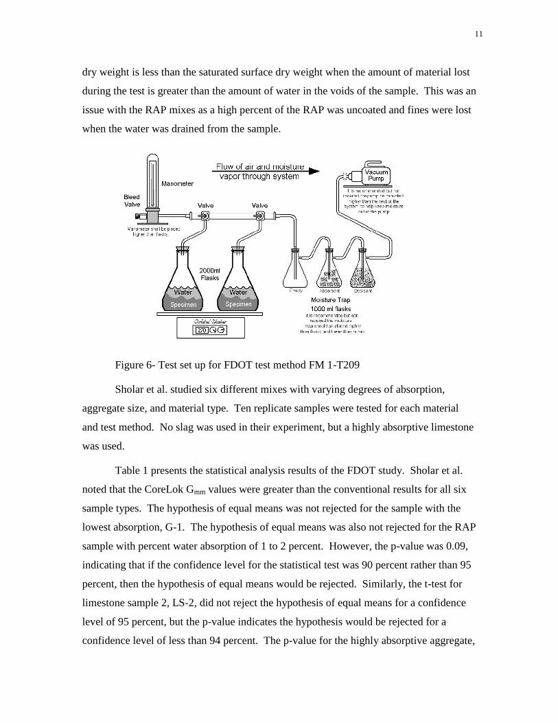
11

dry weight is less than the saturated surface dry weight when the amount of material lost

during the test is greater than the amount of water in the voids of the sample. This was an

issue with the RAP mixes as a high percent of the RAP was uncoated and fines were lost

when the water was drained from the sample.

Figure 6- Test set up for FDOT test method FM 1-T209

Sholar et al. studied six different mixes with varying degrees of absorption,

aggregate size, and material type. Ten replicate samples were tested for each material

and test method. No slag was used in their experiment, but a highly absorptive limestone

was used.

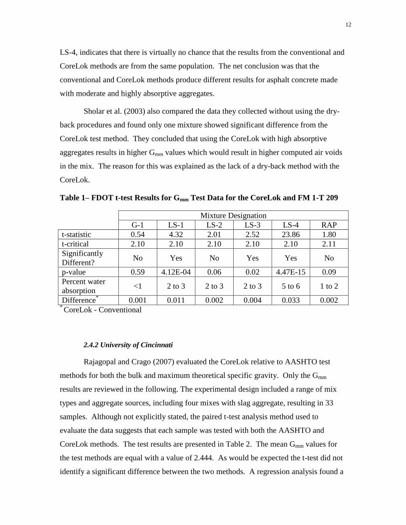
Table 1 presents the statistical analysis results of the FDOT study. Sholar et al.

noted that the CoreLok Gmm values were greater than the conventional results for all six

sample types. The hypothesis of equal means was not rejected for the sample with the

lowest absorption, G-1. The hypothesis of equal means was also not rejected for the RAP

sample with percent water absorption of 1 to 2 percent. However, the p-value was 0.09,

indicating that if the confidence level for the statistical test was 90 percent rather than 95

percent, then the hypothesis of equal means would be rejected. Similarly, the t-test for

limestone sample 2, LS-2, did not reject the hypothesis of equal means for a confidence

level of 95 percent, but the p-value indicates the hypothesis would be rejected for a

confidence level of less than 94 percent. The p-value for the highly absorptive aggregate,

12

LS-4, indicates that there is virtually no chance that the results from the conventional and

CoreLok methods are from the same population. The net conclusion was that the

conventional and CoreLok methods produce different results for asphalt concrete made

with moderate and highly absorptive aggregates.

Sholar et al. (2003) also compared the data they collected without using the dry-

back procedures and found only one mixture showed significant difference from the

CoreLok test method. They concluded that using the CoreLok with high absorptive

aggregates results in higher Gmm values which would result in higher computed air voids

in the mix. The reason for this was explained as the lack of a dry-back method with the

CoreLok.

Table 1– FDOT t-test Results for Gmm Test Data for the CoreLok and FM 1-T 209

Mixture Designation

G-1 LS-1 LS-2 LS-3 LS-4 RAP

t-statistic 0.54 4.32 2.01 2.52 23.86 1.80

t-critical 2.10 2.10 2.10 2.10 2.10 2.11

Significantly

Different? No Yes No Yes Yes No

p-value 0.59 4.12E-04 0.06 0.02 4.47E-15 0.09

Percent water

absorption <1 2 to 3 2 to 3 2 to 3 5 to 6 1 to 2

Difference* 0.001 0.011 0.002 0.004 0.033 0.002

* CoreLok - Conventional

2.4.2 University of Cincinnati

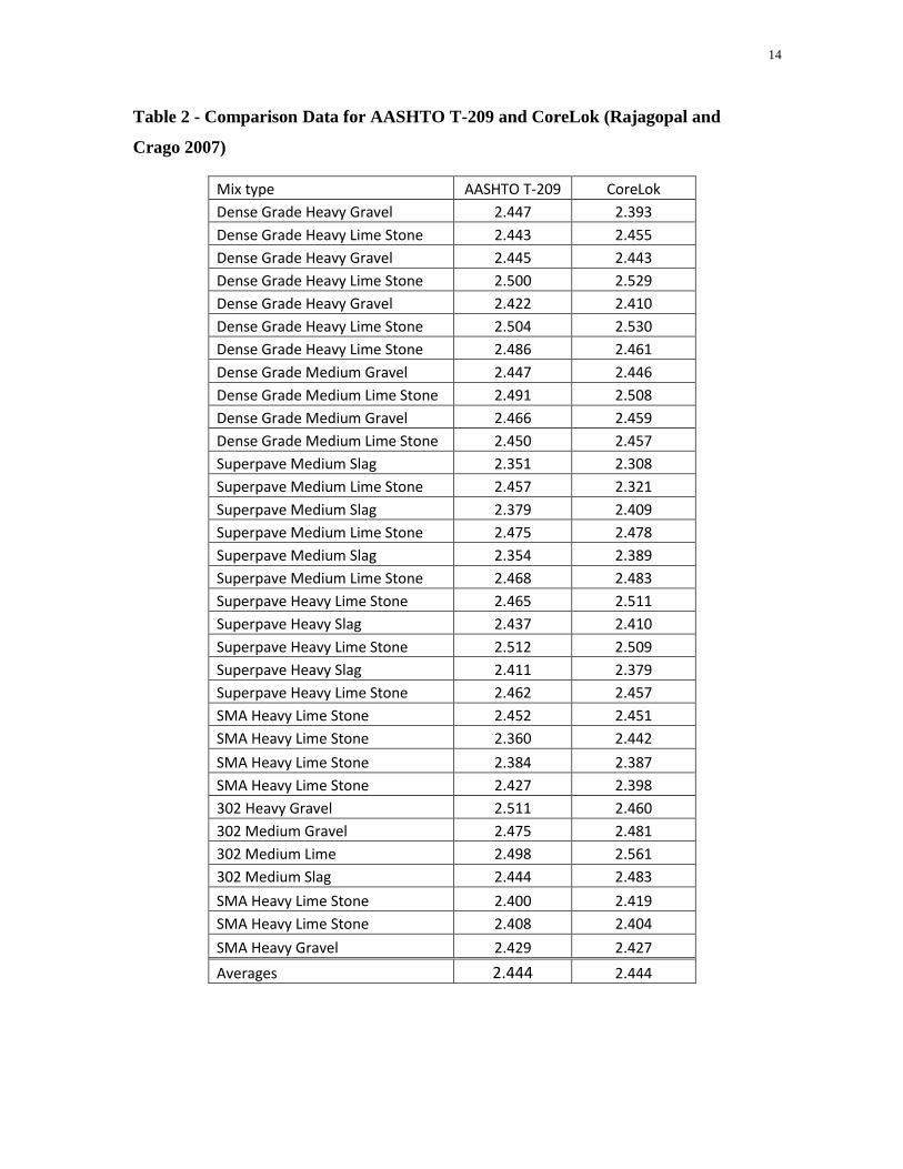
Rajagopal and Crago (2007) evaluated the CoreLok relative to AASHTO test

methods for both the bulk and maximum theoretical specific gravity. Only the Gmm

results are reviewed in the following. The experimental design included a range of mix

types and aggregate sources, including four mixes with slag aggregate, resulting in 33

samples. Although not explicitly stated, the paired t-test analysis method used to

evaluate the data suggests that each sample was tested with both the AASHTO and

CoreLok methods. The test results are presented in Table 2. The mean Gmm values for

the test methods are equal with a value of 2.444. As would be expected the t-test did not

identify a significant difference between the two methods. A regression analysis found a

13

strong correlation between the two methods, with an r value of 0.53. However, the slope

of the regression was 0.92 which indicates the results from the CoreLok are lower than

T-209 for low Gmm values and vice versa for high Gmm values.

14

Table 2 - Comparison Data for AASHTO T-209 and CoreLok (Rajagopal and

Crago 2007)

Mix type AASHTO T-209 CoreLok

Dense Grade Heavy Gravel 2.447 2.393

Dense Grade Heavy Lime Stone 2.443 2.455






Dense Grade Medium Gravel 2.447 2.446

Dense Grade Medium Lime Stone 2.491 2.508

Dense Grade Medium Gravel 2.466 2.459

Dense Grade Medium Lime Stone 2.450 2.457

Superpave Medium Slag 2.351 2.308

Superpave Medium Lime Stone 2.457 2.321





Superpave Heavy Lime Stone 2.465 2.511

Superpave Heavy Slag 2.437 2.410


Superpave Heavy Slag 2.411 2.379


SMA Heavy Lime Stone 2.452 2.451




302 Heavy Gravel 2.511 2.460

302 Medium Gravel 2.475 2.481

302 Medium Lime 2.498 2.561

302 Medium Slag 2.444 2.483



SMA Heavy Gravel 2.429 2.427

Averages 2.444 2.444

15

Chapter 3 Research Methodology

3.1 Introduction

The experimental plan was designed to evaluate differences in maximum

theoretical specific gravity between lab produced and plant produced mixes with a blend

of slag and limestone aggregates. Maximum theoretical gravity was measured using the

conventional (Rice), dry-back, and CoreLok methods. The materials for this experiment

were provided by West Virginia Paving. The asphalt cement was a PG 64-22. The three

types of stones were limestone sand, a No. 8 slag, and a No. 8 limestone.

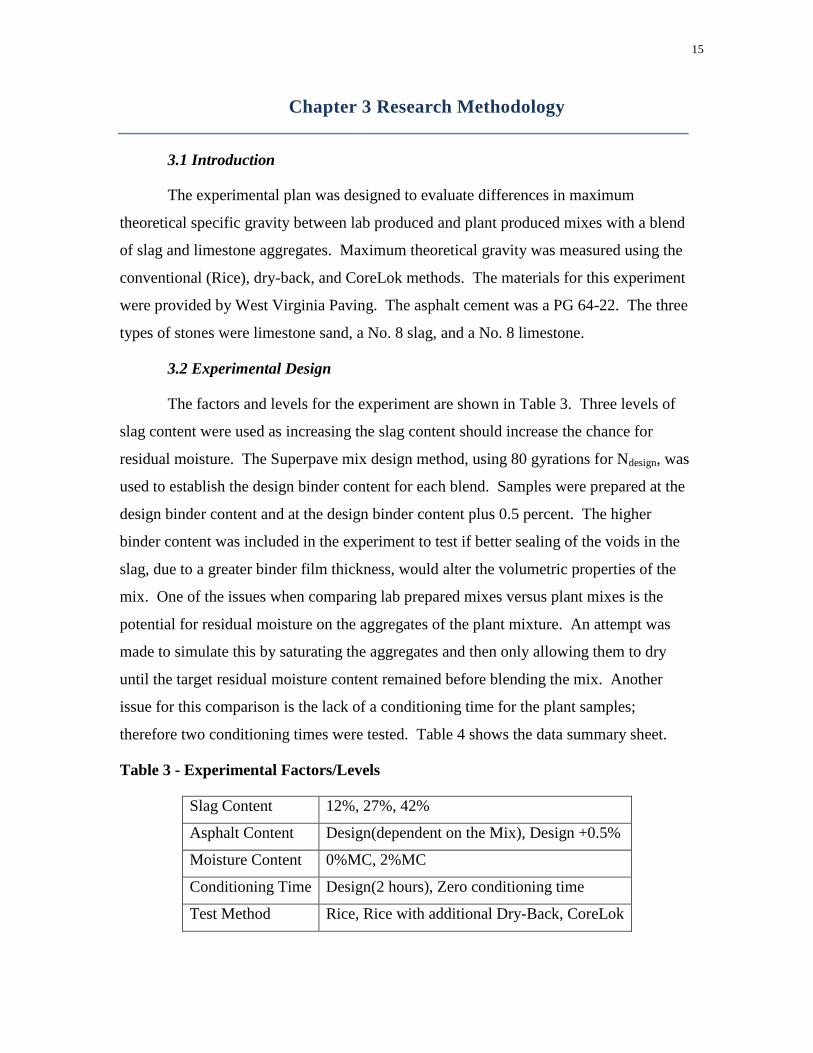
3.2 Experimental Design

The factors and levels for the experiment are shown in Table 3. Three levels of

slag content were used as increasing the slag content should increase the chance for

residual moisture. The Superpave mix design method, using 80 gyrations for Ndesign, was

used to establish the design binder content for each blend. Samples were prepared at the

design binder content and at the design binder content plus 0.5 percent. The higher

binder content was included in the experiment to test if better sealing of the voids in the

slag, due to a greater binder film thickness, would alter the volumetric properties of the

mix. One of the issues when comparing lab prepared mixes versus plant mixes is the

potential for residual moisture on the aggregates of the plant mixture. An attempt was

made to simulate this by saturating the aggregates and then only allowing them to dry

until the target residual moisture content remained before blending the mix. Another

issue for this comparison is the lack of a conditioning time for the plant samples;

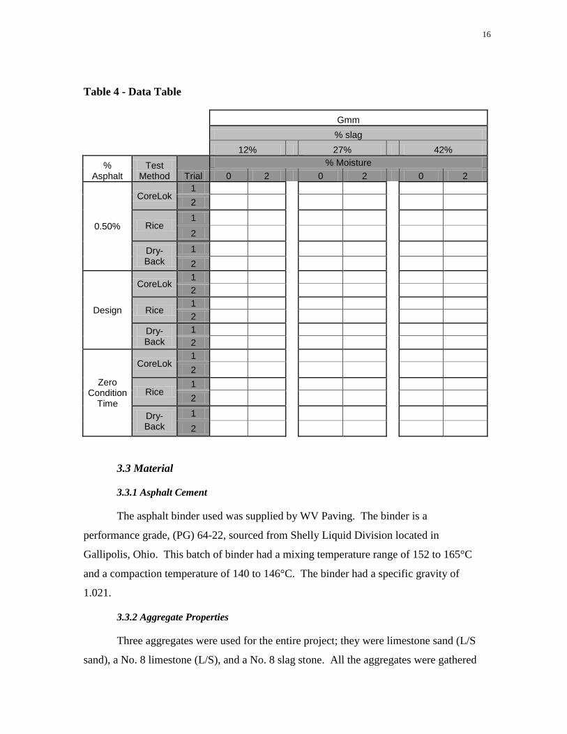
therefore two conditioning times were tested. Table 4 shows the data summary sheet.

Table 3 - Experimental Factors/Levels

Slag Content 12%, 27%, 42%

Asphalt Content Design(dependent on the Mix), Design +0.5%

Moisture Content 0%MC, 2%MC

Conditioning Time Design(2 hours), Zero conditioning time

Test Method Rice, Rice with additional Dry-Back, CoreLok

16

Table 4 - Data Table

Gmm

% slag

12% 27% 42%

% Asphalt

Test Method Trial

% Moisture

0 2 0 2 0 2

0.50%

CoreLok 1

2

Rice 1

2

Dry-Back

1

2

Design

CoreLok 1

2

Rice 1

2

Dry-Back

1

2

Zero Condition

Time

CoreLok 1

2

Rice 1

2

Dry-Back

1

2

3.3 Material

3.3.1 Asphalt Cement

The asphalt binder used was supplied by WV Paving. The binder is a

performance grade, (PG) 64-22, sourced from Shelly Liquid Division located in

Gallipolis, Ohio. This batch of binder had a mixing temperature range of 152 to 165°C

and a compaction temperature of 140 to 146°C. The binder had a specific gravity of

1.021.

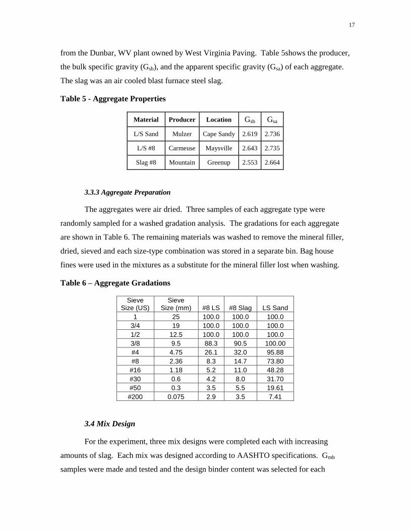
3.3.2 Aggregate Properties

Three aggregates were used for the entire project; they were limestone sand (L/S

sand), a No. 8 limestone (L/S), and a No. 8 slag stone. All the aggregates were gathered

17

from the Dunbar, WV plant owned by West Virginia Paving. Table 5shows the producer,

the bulk specific gravity (Gsb), and the apparent specific gravity (Gsa) of each aggregate.

The slag was an air cooled blast furnace steel slag.

Table 5 - Aggregate Properties

Material Producer Location Gsb Gsa

L/S Sand Mulzer Cape Sandy 2.619 2.736

L/S #8 Carmeuse Maysville 2.643 2.735

Slag #8 Mountain Greenup 2.553 2.664

3.3.3 Aggregate Preparation

The aggregates were air dried. Three samples of each aggregate type were

randomly sampled for a washed gradation analysis. The gradations for each aggregate

are shown in Table 6. The remaining materials was washed to remove the mineral filler,

dried, sieved and each size-type combination was stored in a separate bin. Bag house

fines were used in the mixtures as a substitute for the mineral filler lost when washing.

Table 6 – Aggregate Gradations

Sieve Size (US)

Sieve Size (mm) #8 LS #8 Slag LS Sand

1 25 100.0 100.0 100.0

3/4 19 100.0 100.0 100.0

1/2 12.5 100.0 100.0 100.0

3/8 9.5 88.3 90.5 100.00

#4 4.75 26.1 32.0 95.88

#8 2.36 8.3 14.7 73.80

#16 1.18 5.2 11.0 48.28

#30 0.6 4.2 8.0 31.70

#50 0.3 3.5 5.5 19.61

#200 0.075 2.9 3.5 7.41

3.4 Mix Design

For the experiment, three mix designs were completed each with increasing

amounts of slag. Each mix was designed according to AASHTO specifications. Gmb

samples were made and tested and the design binder content was selected for each

18

mixture. The binder content for each mix was 6.2% for low slag, 6.5% for medium slag,

and 7.0% for high slag content.

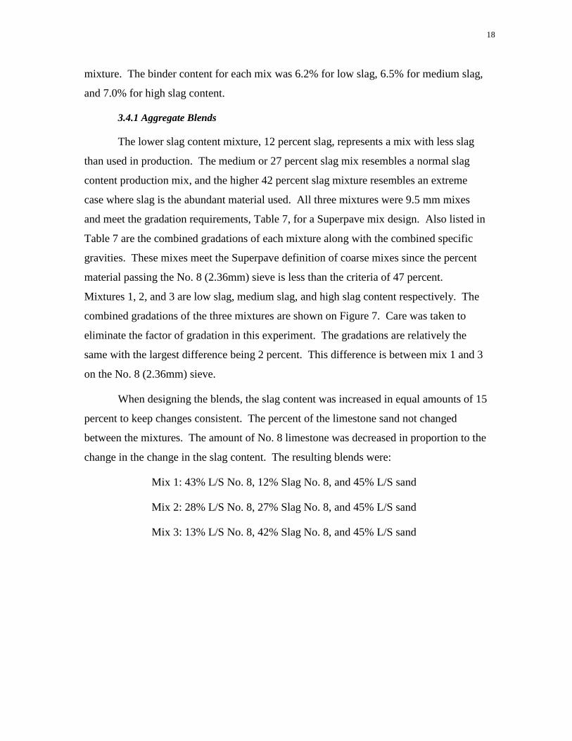
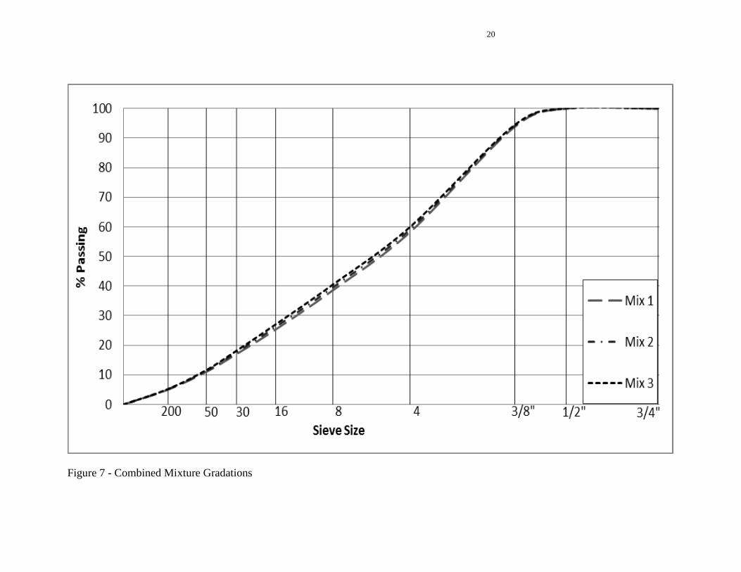
3.4.1 Aggregate Blends

The lower slag content mixture, 12 percent slag, represents a mix with less slag

than used in production. The medium or 27 percent slag mix resembles a normal slag

content production mix, and the higher 42 percent slag mixture resembles an extreme

case where slag is the abundant material used. All three mixtures were 9.5 mm mixes

and meet the gradation requirements, Table 7, for a Superpave mix design. Also listed in

Table 7 are the combined gradations of each mixture along with the combined specific

gravities. These mixes meet the Superpave definition of coarse mixes since the percent

material passing the No. 8 (2.36mm) sieve is less than the criteria of 47 percent.

Mixtures 1, 2, and 3 are low slag, medium slag, and high slag content respectively. The

combined gradations of the three mixtures are shown on Figure 7. Care was taken to

eliminate the factor of gradation in this experiment. The gradations are relatively the

same with the largest difference being 2 percent. This difference is between mix 1 and 3

on the No. 8 (2.36mm) sieve.

When designing the blends, the slag content was increased in equal amounts of 15

percent to keep changes consistent. The percent of the limestone sand not changed

between the mixtures. The amount of No. 8 limestone was decreased in proportion to the

change in the change in the slag content. The resulting blends were:

Mix 1: 43% L/S No. 8, 12% Slag No. 8, and 45% L/S sand



19

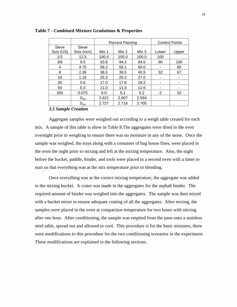
Table 7 - Combined Mixture Gradations & Properties

Percent Passing Control Points

Sieve Size (US)

Sieve Size (mm) Mix 1 Mix 2 Mix 3 Lower Upper

1/2 12.5 100.0 100.0 100.0 100

3/8 9.5 93.8 94.2 94.5 90 100

4 4.75 58.2 59.1 60.0 - 90

8 2.36 38.5 39.5 40.5 32 67

16 1.18 25.3 26.2 27.0 - -

30 0.6 17.0 17.6 18.2 - -

50 0.3 11.0 11.3 11.6 - -

200 0.075 5.0 5.1 5.2 2 10

Gsb 2.621 2.607 2.594

Gsa 2.727 2.716 2.705

3.5 Sample Creation

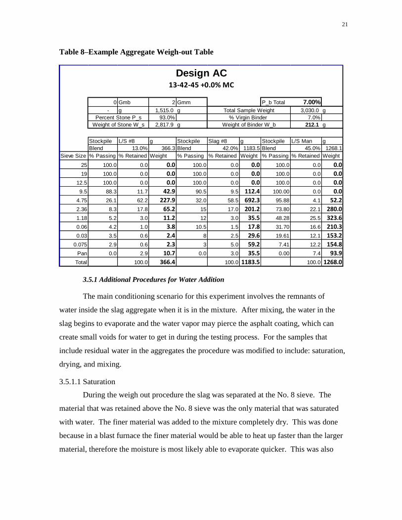
Aggregate samples were weighed out according to a weigh table created for each

mix. A sample of this table is show in Table 8.The aggregates were dried in the oven

overnight prior to weighing to ensure there was no moisture in any of the stone. Once the

sample was weighed, the trays along with a container of bag house fines, were placed in

the oven the night prior to mixing and left at the mixing temperature. Also, the night

before the bucket, paddle, binder, and tools were placed in a second oven with a timer to

start so that everything was at the mix temperature prior to blending.

Once everything was at the correct mixing temperature, the aggregate was added

to the mixing bucket. A crater was made in the aggregates for the asphalt binder. The

required amount of binder was weighed into the aggregates. The sample was then mixed

with a bucket mixer to ensure adequate coating of all the aggregates. After mixing, the

samples were placed in the oven at compaction temperature for two hours with stirring

after one hour. After conditioning, the sample was emptied from the pans onto a stainless

steel table, spread out and allowed to cool. This procedure is for the basic mixtures, there

were modifications to this procedure for the two conditioning scenarios in the experiment.

These modifications are explained in the following sections.

20

Figure 7 - Combined Mixture Gradations

21

Table 8–Example Aggregate Weigh-out Table

3.5.1 Additional Procedures for Water Addition

The main conditioning scenario for this experiment involves the remnants of

water inside the slag aggregate when it is in the mixture. After mixing, the water in the

slag begins to evaporate and the water vapor may pierce the asphalt coating, which can

create small voids for water to get in during the testing process. For the samples that

include residual water in the aggregates the procedure was modified to include: saturation,

drying, and mixing.

3.5.1.1 Saturation

During the weigh out procedure the slag was separated at the No. 8 sieve. The

material that was retained above the No. 8 sieve was the only material that was saturated

with water. The finer material was added to the mixture completely dry. This was done

because in a blast furnace the finer material would be able to heat up faster than the larger

material, therefore the moisture is most likely able to evaporate quicker. This was also

0 Gmb 2 Gmm P_b Total 7.00%

- g 1,515.0 g 3,030.0 g

93.0% 7.0%

2,817.9 g 212.1 g

Stockpile L/S #8 g Stockpile Slag #8 g Stockpile L/S Man g

Blend 13.0% 366.3 Blend 42.0% 1183.5 Blend 45.0% 1268.1

Sieve Size % Passing % Retained Weight % Passing % Retained Weight % Passing % Retained Weight

25 100.0 0.0 0.0 100.0 0.0 0.0 100.0 0.0 0.0

19 100.0 0.0 0.0 100.0 0.0 0.0 100.0 0.0 0.0

12.5 100.0 0.0 0.0 100.0 0.0 0.0 100.0 0.0 0.0

9.5 88.3 11.7 42.9 90.5 9.5 112.4 100.00 0.0 0.0

4.75 26.1 62.2 227.9 32.0 58.5 692.3 95.88 4.1 52.2

2.36 8.3 17.8 65.2 15 17.0 201.2 73.80 22.1 280.0

1.18 5.2 3.0 11.2 12 3.0 35.5 48.28 25.5 323.6

0.06 4.2 1.0 3.8 10.5 1.5 17.8 31.70 16.6 210.3

0.03 3.5 0.6 2.4 8 2.5 29.6 19.61 12.1 153.2

0.075 2.9 0.6 2.3 3 5.0 59.2 7.41 12.2 154.8

Pan 0.0 2.9 10.7 0.0 3.0 35.5 0.00 7.4 93.9

Total 100.0 366.4 100.0 1183.5 100.0 1268.0

Weight of Binder W_b

Percent Stone P_s

Weight of Stone W_s

Design AC13-42-45 +0.0% MC

Total Sample Weight

% Virgin Binder

22

done so that finer material would not be lost when excess water was emptied from the

tray.

The material retained on the No. 8 sieve was saturated by placing it in a container,

covering with water, and vibrating while a vacuum was applied. The vacuum was set to

55 ± 2.5 mmHg. The sample was subjected to the vacuum for 30 minutes and then

submerged under water for an additional 24 ± 1 hour. The quantity of aggregate for the

high, 42 percent, slag mix was too large to fit in the container, so it was split in half and

each half underwent the vacuum process one after the other and then were submerged

together for the 24 hour period.

3.5.1.2 Drying

The following morning the sample was drained of the excess water. This was

done over a No. 200 sieve to avoid the loss of material. Afterwards the sample was

placed in the oven to heat up and dry to the desired moisture content. The saturated

aggregate was placed in a separate oven from the other materials and bucket. This was

done to limit the heat loss of the other material from opening the oven door to many

times. After the slag had been in the oven for a short time, the weight was taken to see if

it had reached the weight needed for the required two percent moisture content. This two

percent moisture is based on the entire weight of the slag portion of the mixture. For

example if there was 1000 grams of slag in the mix, 20 grams of water was required to be

retained in the material retained above the No. 8 (2.36mm) sieve. The slag was stirred

multiple times during the drying process to resemble what happens to the rocks when

they go through the plant dryer.

3.5.1.3 Mixing

Once the slag had reached the required 2% moisture content it was removed from

the oven and placed in the bucket that was already at the correct mixing temperature. To

avoid further moisture loss, the slag was always placed in the bucket first and quickly

followed by the sand, dust, and limestone. After all the materials were in the bucket it

was weighed and recorded. Then the sample was weighed again after mixing was

completed to see how much water had evaporated during the mixing process.

23

3.5.1 Additional Procedures for Zero Conditioning Time

The other main conditioning scenario investigated was zero conditioning time.

When a sample is taken from the plant it is immediately brought to the lab and tested.

Since this occurs, a shorter conditioning time for lab created samples was examined.

Zero conditioning time was chosen to show the extreme case of the lack of conditioning

in plant produced samples. The only change to the procedure was that the sample was

taken straight from the mixing bucket and spread out on the stainless steel table top. The

samples that had an addition of water to the mix followed the same mixing procedures

that were listed in the above section, but the two hour conditioning time was again

eliminated.

3.6 Sample Testing

After the samples were mixed and conditioned (if required) they were spread on

the table for cooling. While still lukewarm and pliable, the samples were broken apart

into small pieces and stirred to make sure no large clumps formed. The sample was

stirred again after a few minutes and then allowed to cool to near room temperature.

Once the sample cooled, it was gathered into a pile and split into quarters, as per

the AASHTO T-268’s sampling method. The entire sample consisted of two test samples.

Each of these test samples were originally set to weigh 1515 grams. The required sample

size for a Rice test is at least 1500 grams for a 9.5 mm mix, and the CoreLok has a

maximum sample size of 2000 grams. Each sample was then tested with each test

method. The data collected during the dry-back procedure was used for the conventional

Rice method, simply ignoring the weight recorded after the additional dry-back.

24

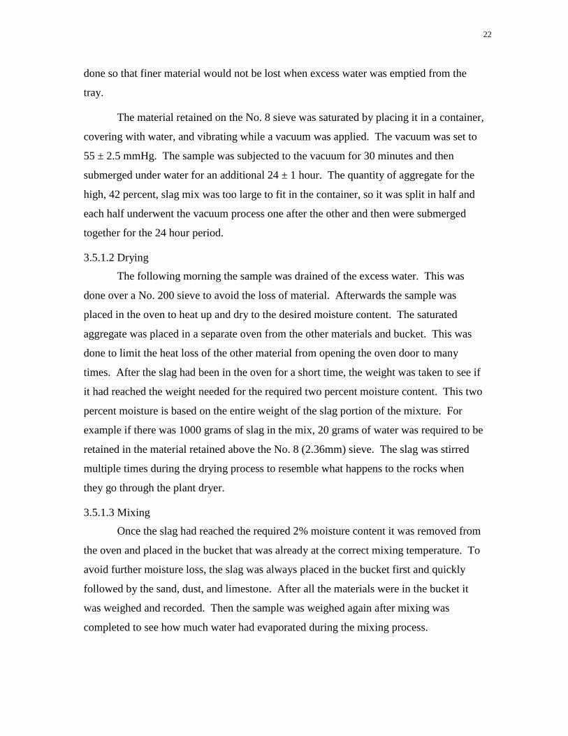
3.6.1 Test Methods

Three test methods were used for this investigation: the conventional AASHTO

T-209 Rice method, the T-209 with additional Dry-Back procedure, and the CoreLok.

Each test was completed using the procedures listed in the respective manuals; are

described in Chapter 2. In order to complete the two test samples for the dry-back

procedure, a drying rack was fabricated that held two No. 30 sieves held at an angle for

each material. A fan was then placed behind each of the sieves and blew air up through

the bottom of the sieves. Figure 8 shows the drying rack.

Figure 8 - Drying Rack

25

Chapter 4 Results and Analysis

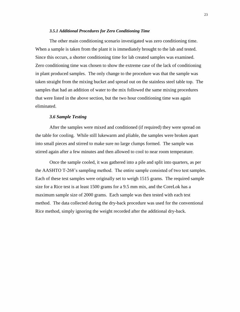
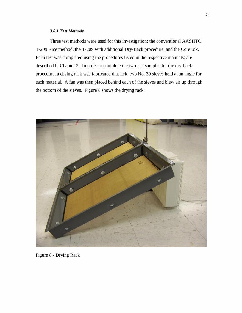
4.1 Introduction

A total of 18 mixes were tested for determining maximum theoretical specific

gravity use CoreLok, and AASHTO’s T-209 method with and without the dry-back

procedures. The factors and levels of the experiment are shown in Table 9. Two samples

were made and used for each testing device, totaling 36 samples and 108 tests. Each

group of results was given an acronym to describe its mixture properties and test

procedure, as defined in Table 10. For example LPCM means Low slag content (12

percent), Plus an additional half percent asphalt, and CoreLok test method, and two

percent Moisture.

Table 9 - Experimental Factors and Levels

% Slag

12% 27% 42%

%Asphalt Conditioning

Test Method

% Moisture

0 2 0 2 0 2

+0.50% 2 hr

CoreLok LPC LPCM MPC MPCM HPC HPCM

RICE LPR LPRM MPR MPRM HPR HPRM

Dry-Back LPD LPDM MPD MPDM HPD HPDM

Design 2 hr

CoreLok LDC LDCM MDC MDCM HDC HDCM

RICE LDR LDRM MDR MDRM HDR HDRM

Dry-Back LDD LDDM MDD MDDM HDD HDDM

Design 0 hr

CoreLok LZC LZCM MZC MZCM HZC HZCM

RICE LZR LZRM MZR MZRM HZR HZRM

Dry-Back LZD LZDM MZD MZDM HZD HZDM

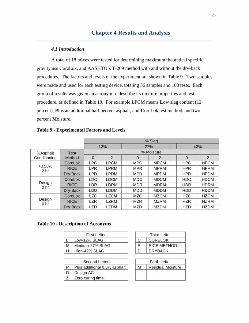
Table 10 - Description of Acronyms

First Letter Third Letter

L Low-12% SLAG C CORELOK

M Medium-27% SLAG R RICE METHOD

H High-42% SLAG D DRYBACK

Second Letter Forth Letter

P Plus additional 0.5% asphalt M Residual Moisture

D Design AC

Z Zero curing time

26

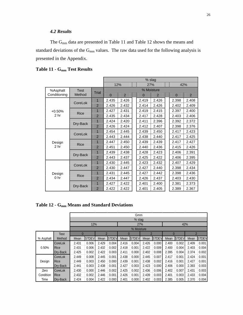
4.2 Results

The Gmm data are presented in Table 11 and Table 12 shows the means and

standard deviations of the Gmm values. The raw data used for the following analysis is

presented in the Appendix.

Table 11 - Gmm Test Results

% slag

12%

27%

42%

%Asphalt Conditioning

Test Method

Trial % Moisture

0 2

0 2

0 2

+0.50% 2 hr

CoreLok 1 2.435 2.426

2.419 2.426

2.398 2.408

2 2.426 2.432

2.414 2.426

2.402 2.409

Rice 1 2.427 2.431

2.419 2.415

2.397 2.400

2 2.435 2.434

2.417 2.428

2.403 2.406

Dry-Back 1 2.424 2.420

2.411 2.396

2.392 2.372

2 2.426 2.424

2.412 2.407

2.398 2.376

Design 2 hr

CoreLok 1 2.454 2.445

2.439 2.450

2.417 2.423

2 2.443 2.444

2.438 2.440

2.417 2.425

Rice 1 2.447 2.450

2.439 2.439

2.417 2.427

2 2.451 2.450

2.440 2.436

2.415 2.426

Dry-Back 1 2.439 2.438

2.428 2.423

2.406 2.391

2 2.443 2.437

2.425 2.422

2.406 2.395

Design 0 hr

CoreLok 1 2.430 2.445

2.423 2.432

2.407 2.429

2 2.430 2.447

2.427 2.440

2.398 2.434

Rice 1 2.431 2.445

2.427 2.442

2.398 2.436

2 2.434 2.447

2.426 2.437

2.403 2.430

Dry-Back 1 2.427 2.422

2.401 2.400

2.381 2.373

2 2.422 2.422

2.401 2.405

2.389 2.367

Table 12 - Gmm Means and Standard Deviations

Mean STDEV Mean STDEV Mean STDEV Mean STDEV Mean STDEV Mean STDEV

CoreLok 2.431 0.006 2.429 0.004 2.416 0.004 2.426 0.000 2.400 0.002 2.409 0.001

Rice 2.431 0.006 2.432 0.002 2.418 0.001 2.422 0.009 2.400 0.004 2.403 0.004

Dry-Back 2.425 0.002 2.422 0.003 2.411 0.000 2.402 0.008 2.395 0.004 2.374 0.002

CoreLok 2.449 0.008 2.445 0.001 2.438 0.000 2.445 0.007 2.417 0.001 2.424 0.001

Rice 2.449 0.003 2.450 0.000 2.439 0.001 2.438 0.002 2.416 0.001 2.427 0.001

Dry-Back 2.441 0.003 2.438 0.001 2.427 0.003 2.423 0.000 2.406 0.000 2.393 0.003

CoreLok 2.430 0.000 2.446 0.002 2.425 0.002 2.436 0.006 2.402 0.007 2.431 0.003

Rice 2.432 0.002 2.446 0.001 2.426 0.001 2.439 0.003 2.401 0.003 2.433 0.004

Dry-Back 2.424 0.004 2.422 0.000 2.401 0.000 2.402 0.003 2.385 0.005 2.370 0.004

Gmm

0 2

Zero

Condition

Time

Design

% Moisture

% slag

% Asphalt

Test

Method

12% 27% 42%

0 2 0 2

0.50%

27

4.2.1 Gmm Analysis of Test Methods

If the three test methods are equally effective at measuring Gmm then they should

produce equal results. The t-test, used to compare means when fewer than 30

observations are available, evaluates if the null hypothesis, Hn, of equal means can be

rejected for a certain confidence level. The alternative hypothesis, Ho, is for non-equal

means. The decision provided by the t-test is either to reject the null hypothesis or there is

insufficient evidence to reject the null hypotheses. The t-test does not determine if the

null hypothesis should be accepted, but this is the implication of not rejecting the null

hypothesis. A confidence level of 95% was used for the decision for all of the following

statistical analysis. An inherent assumption of the t-test is the data are normally

distributed. The following analysis was performed on the average of two replicate

observations. In this situation the central limits theorem applies which justifies the

normality assumption.

4.2.1.1 Rice versus CoreLok

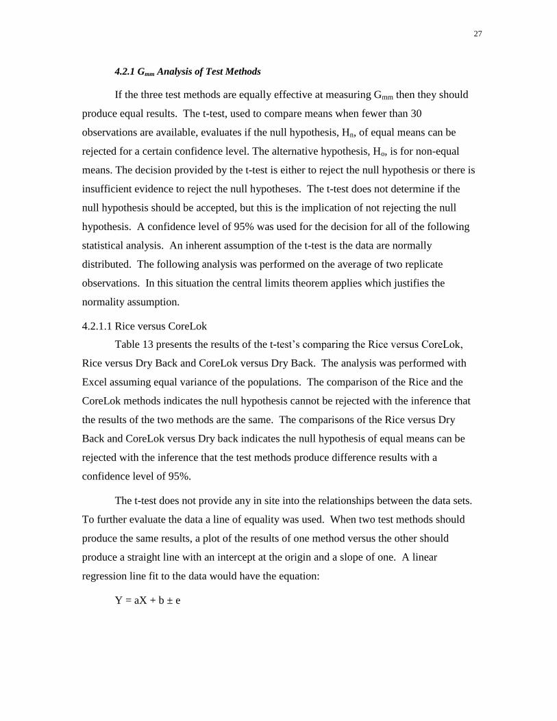
Table 13 presents the results of the t-test’s comparing the Rice versus CoreLok,

Rice versus Dry Back and CoreLok versus Dry Back. The analysis was performed with

Excel assuming equal variance of the populations. The comparison of the Rice and the

CoreLok methods indicates the null hypothesis cannot be rejected with the inference that

the results of the two methods are the same. The comparisons of the Rice versus Dry

Back and CoreLok versus Dry back indicates the null hypothesis of equal means can be

rejected with the inference that the test methods produce difference results with a

confidence level of 95%.

The t-test does not provide any in site into the relationships between the data sets.

To further evaluate the data a line of equality was used. When two test methods should

produce the same results, a plot of the results of one method versus the other should

produce a straight line with an intercept at the origin and a slope of one. A linear

regression line fit to the data would have the equation:

Y = aX + b ± e

28

Where a is the slope of the line and b is the intercept and e is the standard error.

The coefficients can then be tested to determine if a = 1 and b = 0 for a given confidence

level.

Table 13 - t-test comparisons of test methods

Rice CoreLok Dry-Back CoreLok Dry-Back Rice

Mean 2.428 2.428 2.409 2.428 2.409 2.428

Variance 0.000241 0.000214 0.000409 0.000214 0.000409 0.000241

Observations 36 36 36 36 36 36

Pooled Variance 0.000228 0.000312 0.000325 Hypothesized Mean Difference 0 0 0

df 70 70 70

t Stat 0.044 -4.501 -4.444

P(T<=t) one-tail 0.482 0.000 0.000

t Critical one-tail 1.667 1.667 1.667

P(T<=t) two-tail 0.965 0.000 0.000

t Critical two-tail 1.994 1.994 1.994

Decision cannot reject Hn reject Hn reject Hn

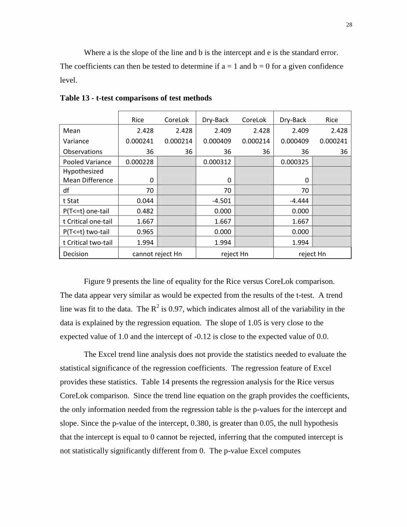
Figure 9 presents the line of equality for the Rice versus CoreLok comparison.

The data appear very similar as would be expected from the results of the t-test. A trend

line was fit to the data. The R2 is 0.97, which indicates almost all of the variability in the

data is explained by the regression equation. The slope of 1.05 is very close to the

expected value of 1.0 and the intercept of -0.12 is close to the expected value of 0.0.

The Excel trend line analysis does not provide the statistics needed to evaluate the

statistical significance of the regression coefficients. The regression feature of Excel

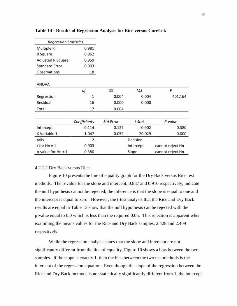
provides these statistics. Table 14 presents the regression analysis for the Rice versus

CoreLok comparison. Since the trend line equation on the graph provides the coefficients,

the only information needed from the regression table is the p-values for the intercept and

slope. Since the p-value of the intercept, 0.380, is greater than 0.05, the null hypothesis

that the intercept is equal to 0 cannot be rejected, inferring that the computed intercept is

not statistically significantly different from 0. The p-value Excel computes

29

Figure 9 - Line of Equality Chart for Rice versus CoreLok Gmm Results.

for the intercept is for a null hypothesis of 0. A supplemental calculation is required to

test for a null hypothesis of the slope equal to 1. The adjusted t-value for a slope of 1 is

computed as:

t = (Slope – 1)/(Standard Error)

Then the p-value is computed using the TDIST function using the adjusted t-value,

the residual degrees of freedom and the two tail assumption as the arguments for the

function. In Table 14 the computed p-value is 0.380. Since this value is greater than

0.05 the null hypothesis cannot be rejected, inferring that the regression slope is not

statistically different from 1.0.

The line of equality analysis results, shown in Table 14 agree with the t-value

analysis in that the conclusion is the Rice and CoreLok methods produce results that are

not significantly different. The advantage of the line of equality approach is that the

relationship between the data is shown. In addition, the line of equality approach has the

ability to determine if there is a bias between the two methods as the intercept of the

regression equation.

y = 1.0472x - 0.1145 R² = 0.9616

2.380

2.400

2.420

2.440

2.460

2.380 2.400 2.420 2.440 2.460

Gm

m R

ice

Gmm CoreLok

Line of Equality

30

Table 14 - Results of Regression Analysis for Rice versus CoreLok

Regression Statistics Multiple R 0.981 R Square 0.962 Adjusted R Square 0.959 Standard Error 0.003 Observations 18

ANOVA df SS MS F

Regression 1 0.004 0.004 401.164

Residual 16 0.000 0.000 Total 17 0.004

Coefficients Std Error t Stat P-value

Intercept -0.114 0.127 -0.902 0.380

X Variable 1 1.047 0.052 20.029 0.000

tails 2

Decision t for Hn = 1 0.903

Intercept cannot reject Hn

p-value for Hn = 1 0.380 Slope cannot reject Hn

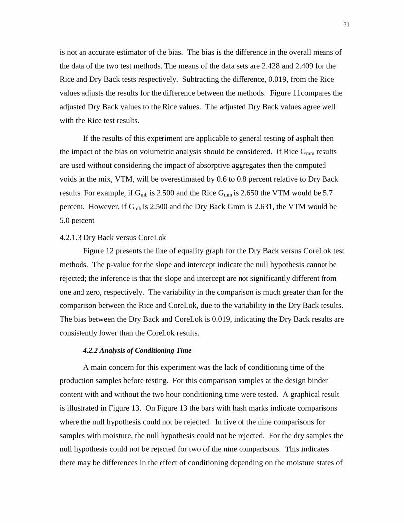
4.2.1.2 Dry Back versus Rice

Figure 10 presents the line of equality graph for the Dry Back versus Rice test

methods. The p-value for the slope and intercept, 0.887 and 0.910 respectively, indicate

the null hypothesis cannot be rejected; the inference is that the slope is equal to one and

the intercept is equal to zero. However, the t-test analysis that the Rice and Dry Back

results are equal in Table 13 show that the null hypothesis can be rejected with the

p-value equal to 0.0 which is less than the required 0.05. This rejection is apparent when

examining the means values for the Rice and Dry Back samples, 2.428 and 2.409

respectively.

While the regression analysis states that the slope and intercept are not

significantly different from the line of equality, Figure 10 shows a bias between the two

samples. If the slope is exactly 1, then the bias between the two test methods is the

intercept of the regression equation. Even though the slope of the regression between the

Rice and Dry Back methods is not statistically significantly different from 1, the intercept

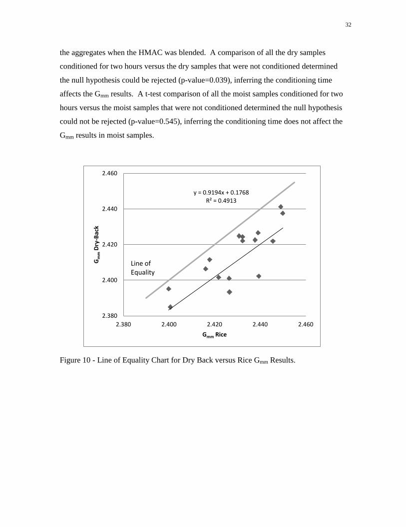
31

is not an accurate estimator of the bias. The bias is the difference in the overall means of

the data of the two test methods. The means of the data sets are 2.428 and 2.409 for the

Rice and Dry Back tests respectively. Subtracting the difference, 0.019, from the Rice

values adjusts the results for the difference between the methods. Figure 11compares the

adjusted Dry Back values to the Rice values. The adjusted Dry Back values agree well

with the Rice test results.

If the results of this experiment are applicable to general testing of asphalt then

the impact of the bias on volumetric analysis should be considered. If Rice Gmm results

are used without considering the impact of absorptive aggregates then the computed

voids in the mix, VTM, will be overestimated by 0.6 to 0.8 percent relative to Dry Back

results. For example, if Gmb is 2.500 and the Rice Gmm is 2.650 the VTM would be 5.7

percent. However, if Gmb is 2.500 and the Dry Back Gmm is 2.631, the VTM would be

5.0 percent

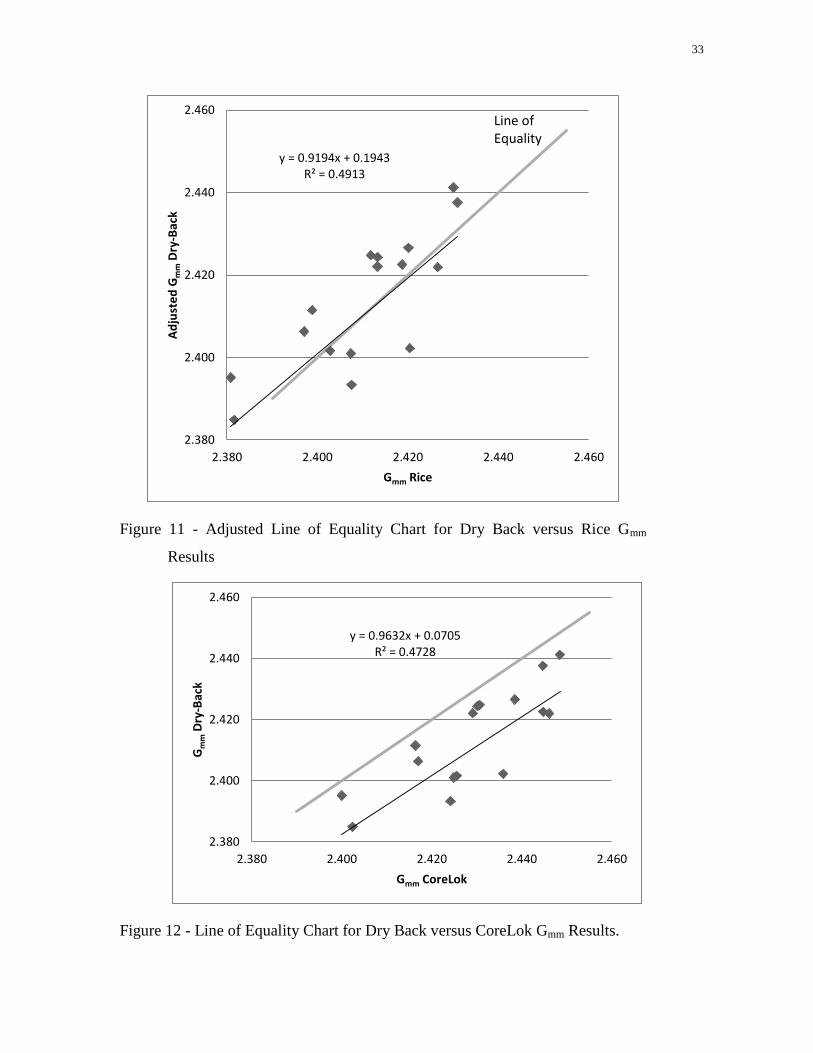
4.2.1.3 Dry Back versus CoreLok

Figure 12 presents the line of equality graph for the Dry Back versus CoreLok test

methods. The p-value for the slope and intercept indicate the null hypothesis cannot be

rejected; the inference is that the slope and intercept are not significantly different from

one and zero, respectively. The variability in the comparison is much greater than for the

comparison between the Rice and CoreLok, due to the variability in the Dry Back results.

The bias between the Dry Back and CoreLok is 0.019, indicating the Dry Back results are

consistently lower than the CoreLok results.

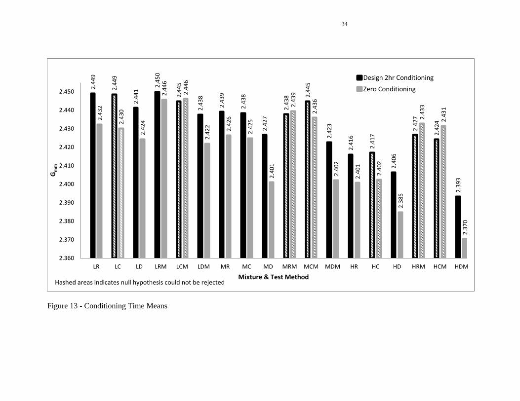
4.2.2 Analysis of Conditioning Time

A main concern for this experiment was the lack of conditioning time of the

production samples before testing. For this comparison samples at the design binder

content with and without the two hour conditioning time were tested. A graphical result

is illustrated in Figure 13. On Figure 13 the bars with hash marks indicate comparisons

where the null hypothesis could not be rejected. In five of the nine comparisons for

samples with moisture, the null hypothesis could not be rejected. For the dry samples the

null hypothesis could not be rejected for two of the nine comparisons. This indicates

there may be differences in the effect of conditioning depending on the moisture states of

32

the aggregates when the HMAC was blended. A comparison of all the dry samples

conditioned for two hours versus the dry samples that were not conditioned determined

the null hypothesis could be rejected (p-value=0.039), inferring the conditioning time

affects the Gmm results. A t-test comparison of all the moist samples conditioned for two

hours versus the moist samples that were not conditioned determined the null hypothesis

could not be rejected (p-value=0.545), inferring the conditioning time does not affect the

Gmm results in moist samples.

Figure 10 - Line of Equality Chart for Dry Back versus Rice Gmm Results.

y = 0.9194x + 0.1768 R² = 0.4913

2.380

2.400

2.420

2.440

2.460

2.380 2.400 2.420 2.440 2.460

Gm

m D

ry-B

ack

Gmm Rice

Line of Equality

33

Figure 11 - Adjusted Line of Equality Chart for Dry Back versus Rice Gmm

Results

Figure 12 - Line of Equality Chart for Dry Back versus CoreLok Gmm Results.

y = 0.9194x + 0.1943 R² = 0.4913

2.380

2.400

2.420

2.440

2.460

2.380 2.400 2.420 2.440 2.460

Ad

just

ed

Gm

m D

ry-B

ack

Gmm Rice

Line of Equality

y = 0.9632x + 0.0705 R² = 0.4728

2.380

2.400

2.420

2.440

2.460

2.380 2.400 2.420 2.440 2.460

Gm

m D

ry-B

ack

Gmm CoreLok

34

Figure 13 - Conditioning Time Means

2.4

49

2.4

49

2.4

41

2.4

50

2.4

45

2.4

38

2.4

39

2.4

38

2.4

27

2.4

38

2.4

45

2.4

23

2.4

16

2.4

17

2.4

06

2.4

27

2.4

24

2.3

93

2.4

32

2.4

30

2.4

24

2.4

46

2.4

46

2.4

22

2.4

26

2.4

25

2.4

01

2.4

39

2.4

36

2.4

02

2.4

01

2.4

02

2.3

85

2.4

33

2.4

31

2.3

70

2.360

2.370

2.380

2.390

2.400

2.410

2.420

2.430

2.440

2.450

LR LC LD LRM LCM LDM MR MC MD MRM MCM MDM HR HC HD HRM HCM HDM

Gm

m

Mixture & Test Method Hashed areas indicates null hypothesis could not be rejected

Design 2hr Conditioning

Zero Conditioning

35

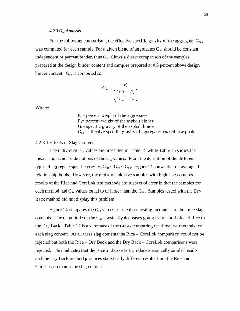
4.2.3 Gse Analysis

For the following comparison, the effective specific gravity of the aggregate, Gse,

was computed for each sample. For a given blend of aggregates Gse should be constant,

independent of percent binder, thus Gse allows a direct comparison of the samples

prepared at the design binder content and samples prepared at 0.5 percent above design

binder content. Gse is computed as:

b

b

mm

sse

G

P

G

PG

100

Where:

Ps = percent weight of the aggregates

Pb= percent weight of the asphalt binder

Gs= specific gravity of the asphalt binder

Gse = effective specific gravity of aggregates coated in asphalt

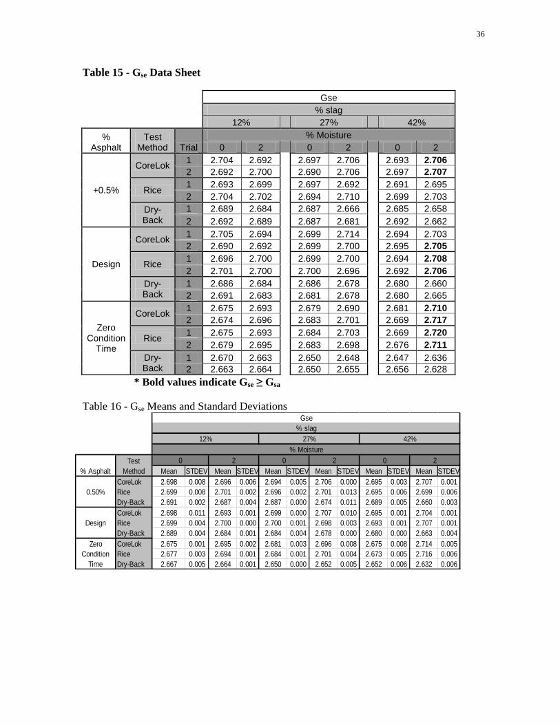
4.2.3.1 Effects of Slag Content

The individual Gse values are presented in Table 15 while Table 16 shows the

means and standard deviations of the Gse values. From the definition of the different

types of aggregate specific gravity, Gsb < Gse < Gsa. Figure 14 shows that on average this

relationship holds. However, the moisture additive samples with high slag contents

results of the Rice and CoreLok test methods are suspect of error in that the samples for

each method had Gse values equal to or larger than the Gsa. Samples tested with the Dry

Back method did not display this problem.

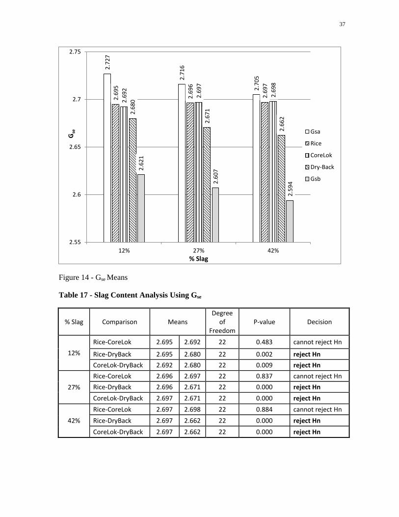
Figure 14 compares the Gse values for the three testing methods and the three slag

contents. The magnitude of the Gse constantly decreases going from CoreLok and Rice to

the Dry Back. Table 17 is a summary of the t-tests comparing the three test methods for

each slag content. At all three slag contents the Rice – CoreLok comparison could not be

rejected but both the Rice – Dry Back and the Dry Back – CoreLok comparisons were

rejected. This indicates that the Rice and CoreLok produce statistically similar results

and the Dry Back method produces statistically different results from the Rice and

CoreLok no matter the slag content.

36

Table 15 - Gse Data Sheet

Gse

% slag

12%

27%

42%

% Asphalt

Test Method Trial

% Moisture

0 2

0 2

0 2

+0.5%

CoreLok 1 2.704 2.692

2.697 2.706

2.693 2.706

2 2.692 2.700

2.690 2.706

2.697 2.707

Rice 1 2.693 2.699

2.697 2.692

2.691 2.695

2 2.704 2.702

2.694 2.710

2.699 2.703

Dry-Back

1 2.689 2.684

2.687 2.666

2.685 2.658

2 2.692 2.689

2.687 2.681

2.692 2.662

Design

CoreLok 1 2.705 2.694

2.699 2.714

2.694 2.703

2 2.690 2.692

2.699 2.700

2.695 2.705

Rice 1 2.696 2.700

2.699 2.700

2.694 2.708

2 2.701 2.700

2.700 2.696

2.692 2.706

Dry-Back

1 2.686 2.684

2.686 2.678

2.680 2.660

2 2.691 2.683

2.681 2.678

2.680 2.665

Zero Condition

Time

CoreLok 1 2.675 2.693

2.679 2.690

2.681 2.710

2 2.674 2.696

2.683 2.701

2.669 2.717

Rice 1 2.675 2.693

2.684 2.703

2.669 2.720

2 2.679 2.695

2.683 2.698

2.676 2.711

Dry-Back

1 2.670 2.663

2.650 2.648

2.647 2.636

2 2.663 2.664

2.650 2.655

2.656 2.628

* Bold values indicate Gse ≥ Gsa

Table 16 - Gse Means and Standard Deviations

Mean STDEV Mean STDEV Mean STDEV Mean STDEV Mean STDEV Mean STDEV

CoreLok 2.698 0.008 2.696 0.006 2.694 0.005 2.706 0.000 2.695 0.003 2.707 0.001

Rice 2.699 0.008 2.701 0.002 2.696 0.002 2.701 0.013 2.695 0.006 2.699 0.006

Dry-Back 2.691 0.002 2.687 0.004 2.687 0.000 2.674 0.011 2.689 0.005 2.660 0.003

CoreLok 2.698 0.011 2.693 0.001 2.699 0.000 2.707 0.010 2.695 0.001 2.704 0.001

Rice 2.699 0.004 2.700 0.000 2.700 0.001 2.698 0.003 2.693 0.001 2.707 0.001

Dry-Back 2.689 0.004 2.684 0.001 2.684 0.004 2.678 0.000 2.680 0.000 2.663 0.004

CoreLok 2.675 0.001 2.695 0.002 2.681 0.003 2.696 0.008 2.675 0.008 2.714 0.005

Rice 2.677 0.003 2.694 0.001 2.684 0.001 2.701 0.004 2.673 0.005 2.716 0.006

Dry-Back 2.667 0.005 2.664 0.001 2.650 0.000 2.652 0.005 2.652 0.006 2.632 0.006

Zero

Condition

Time

2 0 2

0.50%

Design

% Asphalt

Test

Method

0 2 0

% slag

12% 27% 42%

% Moisture

Gse

37

Figure 14 - Gse Means

Table 17 - Slag Content Analysis Using Gse

% Slag Comparison Means Degree

of Freedom

P-value Decision

12%

Rice-CoreLok 2.695 2.692 22 0.483 cannot reject Hn

Rice-DryBack 2.695 2.680 22 0.002 reject Hn

CoreLok-DryBack 2.692 2.680 22 0.009 reject Hn

27%




42%




2.7

27

2.7

16

2.7

05

2.6

95

2.6

96

2.6

97

2.6

92

2.6

97

2.6

98

2.6

80

2.6

71

2.6

62

2.6

21

2.6

07

2.5

94

2.55

2.6

2.65

2.7

2.75

12% 27% 42%

Gse

% Slag

Gsa

Rice

CoreLok

Dry-Back

Gsb

38

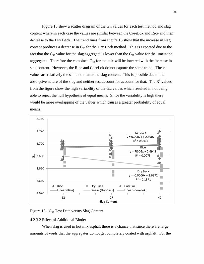
Figure 15 show a scatter diagram of the Gse values for each test method and slag

content where in each case the values are similar between the CoreLok and Rice and then

decrease to the Dry Back. The trend lines from Figure 15 show that the increase in slag

content produces a decrease in Gse for the Dry Back method. This is expected due to the

fact that the Gsb value for the slag aggregate is lower than the Gsb value for the limestone

aggregates. Therefore the combined Gsb for the mix will be lowered with the increase in

slag content. However, the Rice and CoreLok do not capture the same trend. These

values are relatively the same no matter the slag content. This is possible due to the

absorptive nature of the slag and neither test account for account for that. The R2 values

from the figure show the high variability of the Gse values which resulted in not being

able to reject the null hypothesis of equal means. Since the variability is high there

would be more overlapping of the values which causes a greater probability of equal

means.

Figure 15 - Gse Test Data versus Slag Content

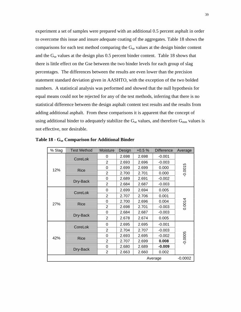
4.2.3.2 Effect of Additional Binder

When slag is used in hot mix asphalt there is a chance that since there are large

amounts of voids that the aggregates do not get completely coated with asphalt. For the

Rice y = 7E-05x + 2.6942

R² = 0.0073

Dry Back y = -0.0006x + 2.6872

R² = 0.1871

CoreLok y = 0.0002x + 2.6907

R² = 0.0464

2.620

2.640

2.660

2.680

2.700

2.720

2.740

7 12 17 22 27 32 37 42

Gse

Slag Content

Rice Dry-Back CoreLok

Linear (Rice) Linear (Dry-Back) Linear (CoreLok)

39

experiment a set of samples were prepared with an additional 0.5 percent asphalt in order

to overcome this issue and insure adequate coating of the aggregates. Table 18 shows the

comparisons for each test method comparing the Gse values at the design binder content

and the Gse values at the design plus 0.5 percent binder content. Table 18 shows that

there is little effect on the Gse between the two binder levels for each group of slag

percentages. The differences between the results are even lower than the precision

statement standard deviation given in AASHTO, with the exception of the two bolded

numbers. A statistical analysis was performed and showed that the null hypothesis for

equal means could not be rejected for any of the test methods, inferring that there is no

statistical difference between the design asphalt content test results and the results from

adding additional asphalt. From these comparisons it is apparent that the concept of

using additional binder to adequately stabilize the Gse values, and therefore Gmm values is

not effective, nor desirable.

Table 18 - Gse Comparison for Additional Binder

% Slag Test Method Moisture Design +0.5 % Difference Average

12%

CoreLok 0 2.698 2.698 -0.001

-0.0

01

5 2 2.693 2.696 -0.003

Rice 0 2.699 2.699 0.000

2 2.700 2.701 0.000

Dry-Back 0 2.689 2.691 -0.002

2 2.684 2.687 -0.003

27%

CoreLok 0 2.699 2.694 0.005

0.0

014

2 2.707 2.706 0.001

Rice 0 2.700 2.696 0.004

2 2.698 2.701 -0.003

Dry-Back 0 2.684 2.687 -0.003

2 2.678 2.674 0.005

42%

CoreLok 0 2.695 2.695 -0.001

-0.0

00

5 2 2.704 2.707 -0.003

Rice 0 2.693 2.695 -0.002

2 2.707 2.699 0.008

Dry-Back 0 2.680 2.689 -0.009

2 2.663 2.660 0.002

Average -0.0002

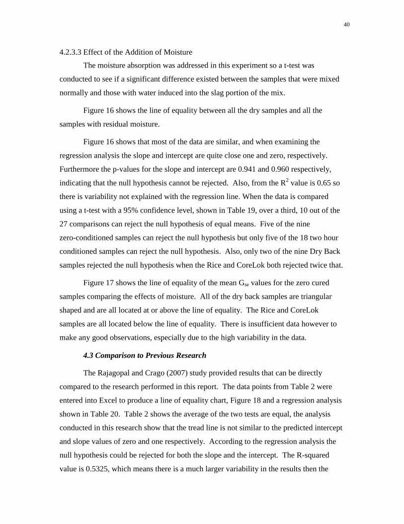
40

4.2.3.3 Effect of the Addition of Moisture

The moisture absorption was addressed in this experiment so a t-test was

conducted to see if a significant difference existed between the samples that were mixed

normally and those with water induced into the slag portion of the mix.

Figure 16 shows the line of equality between all the dry samples and all the

samples with residual moisture.

Figure 16 shows that most of the data are similar, and when examining the

regression analysis the slope and intercept are quite close one and zero, respectively.

Furthermore the p-values for the slope and intercept are 0.941 and 0.960 respectively,

indicating that the null hypothesis cannot be rejected. Also, from the R2 value is 0.65 so

there is variability not explained with the regression line. When the data is compared

using a t-test with a 95% confidence level, shown in Table 19, over a third, 10 out of the

27 comparisons can reject the null hypothesis of equal means. Five of the nine

zero-conditioned samples can reject the null hypothesis but only five of the 18 two hour

conditioned samples can reject the null hypothesis. Also, only two of the nine Dry Back

samples rejected the null hypothesis when the Rice and CoreLok both rejected twice that.

Figure 17 shows the line of equality of the mean Gse values for the zero cured

samples comparing the effects of moisture. All of the dry back samples are triangular

shaped and are all located at or above the line of equality. The Rice and CoreLok

samples are all located below the line of equality. There is insufficient data however to

make any good observations, especially due to the high variability in the data.

4.3 Comparison to Previous Research

The Rajagopal and Crago (2007) study provided results that can be directly

compared to the research performed in this report. The data points from Table 2 were

entered into Excel to produce a line of equality chart, Figure 18 and a regression analysis

shown in Table 20. Table 2 shows the average of the two tests are equal, the analysis

conducted in this research show that the tread line is not similar to the predicted intercept

and slope values of zero and one respectively. According to the regression analysis the

null hypothesis could be rejected for both the slope and the intercept. The R-squared

value is 0.5325, which means there is a much larger variability in the results then the

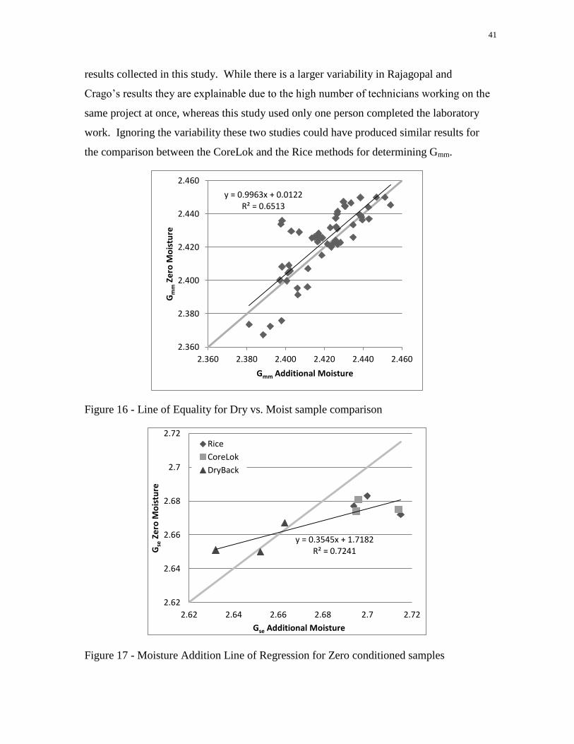
41

results collected in this study. While there is a larger variability in Rajagopal and

Crago’s results they are explainable due to the high number of technicians working on the

same project at once, whereas this study used only one person completed the laboratory

work. Ignoring the variability these two studies could have produced similar results for

the comparison between the CoreLok and the Rice methods for determining Gmm.

Figure 16 - Line of Equality for Dry vs. Moist sample comparison

Figure 17 - Moisture Addition Line of Regression for Zero conditioned samples

y = 0.9963x + 0.0122 R² = 0.6513

2.360

2.380

2.400

2.420

2.440

2.460

2.360 2.380 2.400 2.420 2.440 2.460

Gm

m Z

ero

Mo

istu

re

Gmm Additional Moisture

y = 0.3545x + 1.7182 R² = 0.7241

2.62

2.64

2.66

2.68

2.7

2.72

2.62 2.64 2.66 2.68 2.7 2.72

Gse

Ze

ro M

ois

ture

Gse Additional Moisture

Rice

CoreLok

DryBack

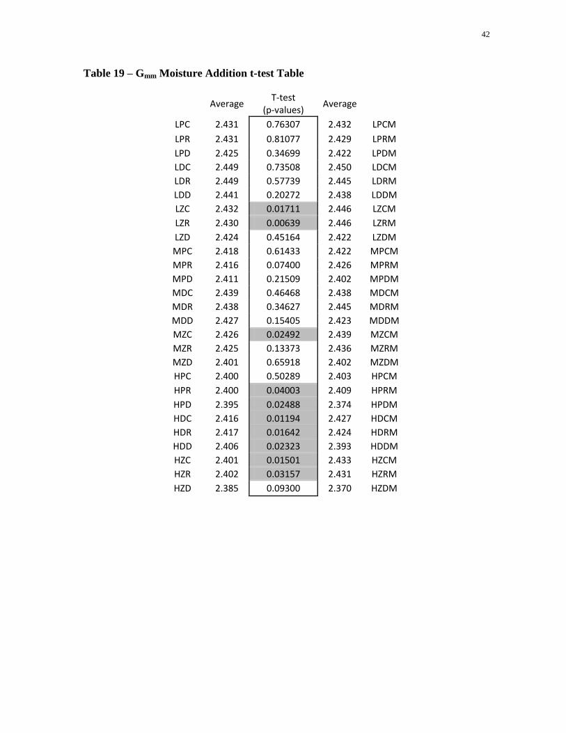
42

Table 19 – Gmm Moisture Addition t-test Table

Average

T-test (p-values)

Average

LPC 2.431 0.76307 2.432 LPCM

LPR 2.431 0.81077 2.429 LPRM

LPD 2.425 0.34699 2.422 LPDM LDC 2.449 0.73508 2.450 LDCM LDR 2.449 0.57739 2.445 LDRM LDD 2.441 0.20272 2.438 LDDM LZC 2.432 0.01711 2.446 LZCM

LZR 2.430 0.00639 2.446 LZRM

LZD 2.424 0.45164 2.422 LZDM MPC 2.418 0.61433 2.422 MPCM

MPR 2.416 0.07400 2.426 MPRM MPD 2.411 0.21509 2.402 MPDM MDC 2.439 0.46468 2.438 MDCM MDR 2.438 0.34627 2.445 MDRM MDD 2.427 0.15405 2.423 MDDM MZC 2.426 0.02492 2.439 MZCM MZR 2.425 0.13373 2.436 MZRM MZD 2.401 0.65918 2.402 MZDM HPC 2.400 0.50289 2.403 HPCM

HPR 2.400 0.04003 2.409 HPRM

HPD 2.395 0.02488 2.374 HPDM HDC 2.416 0.01194 2.427 HDCM HDR 2.417 0.01642 2.424 HDRM HDD 2.406 0.02323 2.393 HDDM HZC 2.401 0.01501 2.433 HZCM HZR 2.402 0.03157 2.431 HZRM

HZD 2.385 0.09300 2.370 HZDM

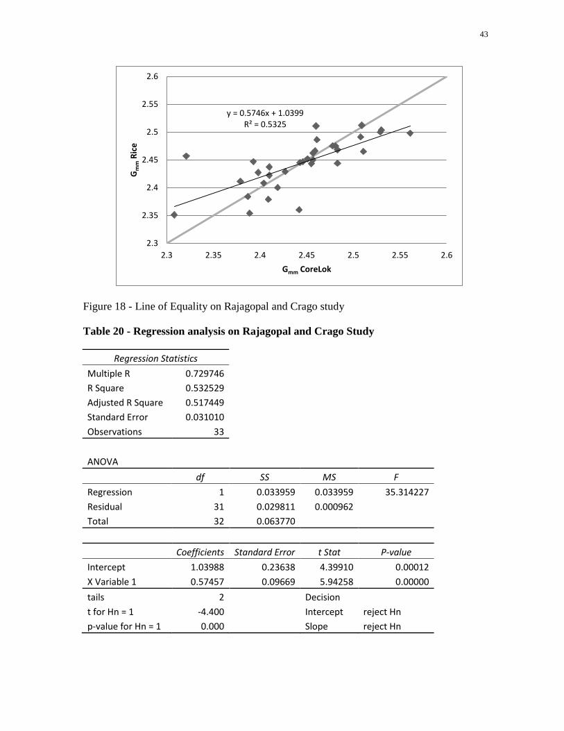
43

Figure 18 - Line of Equality on Rajagopal and Crago study

Table 20 - Regression analysis on Rajagopal and Crago Study

Regression Statistics Multiple R 0.729746 R Square 0.532529 Adjusted R Square 0.517449 Standard Error 0.031010 Observations 33

ANOVA df SS MS F

Regression 1 0.033959 0.033959 35.314227

Residual 31 0.029811 0.000962 Total 32 0.063770

Coefficients Standard Error t Stat P-value

Intercept 1.03988 0.23638 4.39910 0.00012

X Variable 1 0.57457 0.09669 5.94258 0.00000

tails 2

Decision t for Hn = 1 -4.400

Intercept reject Hn

p-value for Hn = 1 0.000 Slope reject Hn

y = 0.5746x + 1.0399 R² = 0.5325

2.3

2.35

2.4

2.45

2.5

2.55

2.6

2.3 2.35 2.4 2.45 2.5 2.55 2.6

Gm

m R

ice

Gmm CoreLok

44

Chapter 5 Conclusions and Recommendations

5.1 Conclusions

The first objective of this study was to determine a possible cause for the difference in

theoretical maximum specific gravity (Gmm) results between a laboratory created sample and

a sample pulled from the production line in the plant. Possible causes thought to affect this

were the residual moisture that is held in the slag after it passes through the drying drum and

the lack of any conditioning time as the samples are pulled from the plant for testing. Both of

these were tested and analyzed.

The analysis compared multiple mixture designs, asphalt contents, and test methods.

The addition of water prior to the mixing procedure revealed minimal influence on the end

values for theoretical maximum specific gravity, only affecting one-third of the values. It is

important to point out that about seventy percent of those affected were found to be in the

high slag content mixture. There was also an increase with the variability of the results when

moisture was induced in the samples. Even though the moisture had an effect on the test data,

overall it was in the wrong direction. The moist samples had Gmm values were higher than

those samples with dry aggregates.

The second theory involving the lack of a conditioning time for plant produced

samples proved to be probable. With 75 percent of the samples showing significant

differences between the standard two hours and the simulated plant produced sample with no

conditioning. There were only two of nine samples without residual moisture that the null

hypothesis could not be rejected, inferring that there is a significant difference between

conditioning times.

The second objective was to determine if the Dry Back procedure was necessary.

According to the Gse results the Dry Back samples were the only samples to account for the

effects of the additional slag. Figure 15 showed that the Dry Back values were the only ones

to decrease as the slag content increase. This indicates the standard method is not capturing

the effect of absorption; hence there is no basis for discontinuing the use of the Dry Back

method at this time.

The final objective was to determine if the CoreLok could replace the Rice test

(AASHTO T-209). The Gmm analysis for the test methods revealed there was a strong

correlation between all the testing methods. The CoreLok showed no statistical difference

from the Rice method results. While there is a strong correlation between the Rice and

45

CoreLok there was bias when comparing the Dry Back to the Rice and CoreLok. The

CoreLok and Rice test methods always overestimate the Dry Back method results. The bias

between the Rice and Dry Back and between the CoreLok and Dry Back were equal to 0.019;

this is interesting because InstroTek claims that the CoreLok eliminates the need for the Dry

Back procedure. Due to these and the results conducted by the University of Cincinnati, it

appears that the CoreLok can be used in lieu of T-209 if there are no absorptive aggregates

being used in the mix design. However, if there are absorptive aggregates then the Dry Back

will need to be used to account for the absorption.

Table 21 is a list of statistical analyses used when comparing the results. Other Gse

analysis was conducted to be able to compare results between design binder content and

samples with the additional 0.5 percent binder more accurately then Gmm can. This is because

Gse is not dependent on the asphalt content like Gmm is. These analyses revealed that adding

additional binder to aid in sealing the stones better had little influence on the end results.

Since Gse had been calculated, F, the absorption factor was calculated. F captures the

difference in the amount of asphalt absorbed in the aggregate compared to the amount of

water absorbed. These values while not included in this report since the analysis would show

the same results the Gse had. However, the data did show that there was a significant

difference from the AASHTO assumed value of 0.8, which may have to do with the high void

content in slag aggregates.

5.2 Recommendations for Further Study

This research was limited to following the certain test procedure associated with the

three test methods used. Knowing this, further research could be conducted to analyze the

potential need for a Dry Back procedure for the CoreLok vacuum sealing device. The

researched mixture designs for this report were limited to only slag No.8, without the use of

slag sands. Further investigations should be conducted to see the

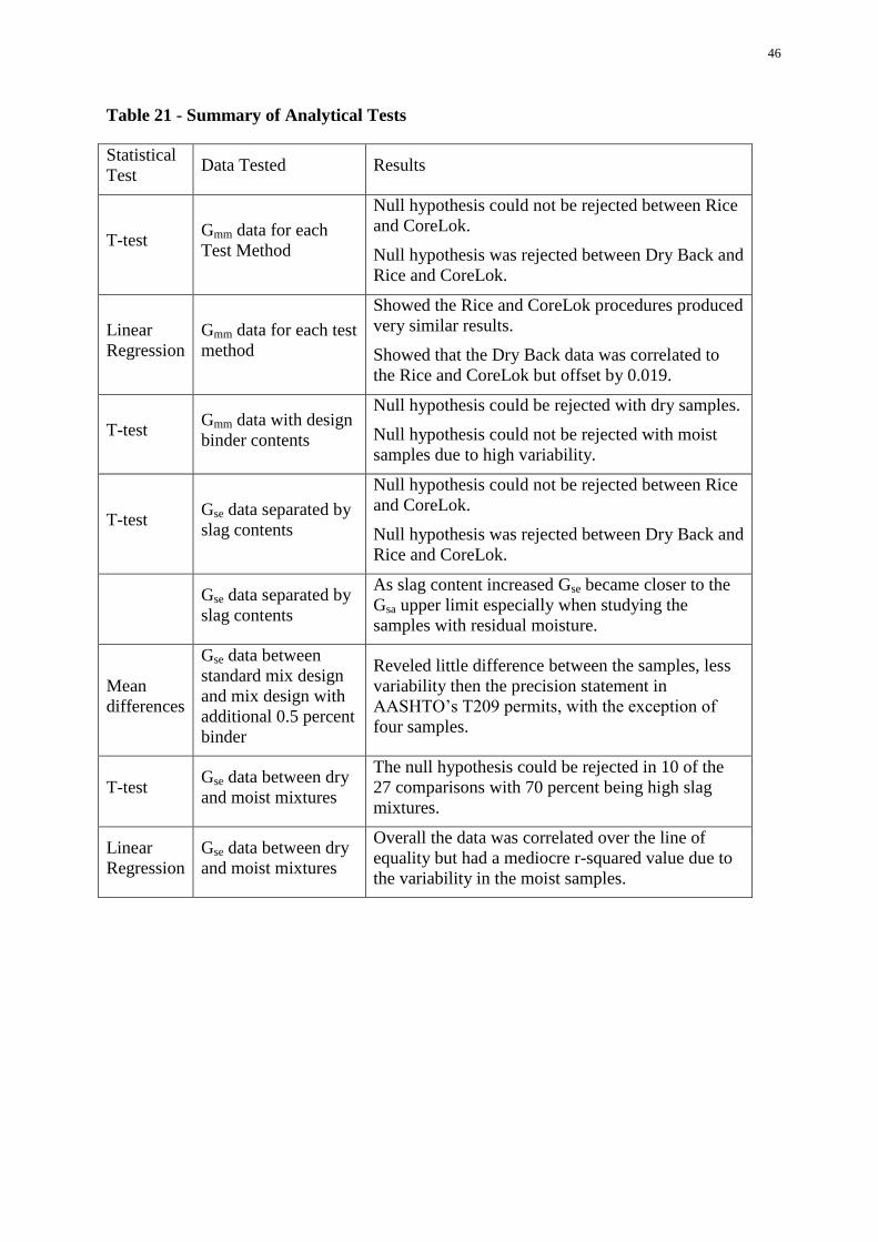
46

Table 21 - Summary of Analytical Tests

Statistical

Test Data Tested Results

T-test Gmm data for each

Test Method

Null hypothesis could not be rejected between Rice

and CoreLok.

Null hypothesis was rejected between Dry Back and

Rice and CoreLok.

Linear

Regression

Gmm data for each test

method

Showed the Rice and CoreLok procedures produced

very similar results.

Showed that the Dry Back data was correlated to

the Rice and CoreLok but offset by 0.019.

T-test Gmm data with design

binder contents

Null hypothesis could be rejected with dry samples.

Null hypothesis could not be rejected with moist

samples due to high variability.

T-test Gse data separated by

slag contents

Null hypothesis could not be rejected between Rice

and CoreLok.

Null hypothesis was rejected between Dry Back and

Rice and CoreLok.

Gse data separated by

slag contents

As slag content increased Gse became closer to the

Gsa upper limit especially when studying the

samples with residual moisture.

Mean

differences

Gse data between

standard mix design

and mix design with

additional 0.5 percent

binder

Reveled little difference between the samples, less

variability then the precision statement in

AASHTO’s T209 permits, with the exception of

four samples.

T-test Gse data between dry

and moist mixtures

The null hypothesis could be rejected in 10 of the

27 comparisons with 70 percent being high slag

mixtures.

Linear

Regression

Gse data between dry

and moist mixtures

Overall the data was correlated over the line of

equality but had a mediocre r-squared value due to

the variability in the moist samples.

47

possible influence that different size aggregates have on the change in testing results. Also,

the addition of slag sand instead of limestone sand could have influence in the Gmm results.

The mixtures were also limited to a maximum of 42 percent slag to resemble a high amount

of slag present in mixtures. From discussions with West Virginia Paving, the highest amount

of course slag they had ever used in a mixture was 50 percent. It is possible that in extreme

cases, where slag is the abundant material, the moisture addition could become even more

apparent.

As conditioning time appears to be a large contributor to the change in theoretical

maximum specific gravity results, further investigations should be done to see the effects at

various times. The research should explore the possibility of adding additional short

conditioning times (15 to 30 minutes) to plant samples to best account for the absorption of

certain aggregates. Also, possible research could be conducted to analyze the absorption

factor, F, for absorbent materials such as slag, that way mix designs can better resemble the

material used.

48

References

FHWA, 1997, User Guidelines for Waste and Byproduct Materials in Pavement

Construction.Blast Furnace Slag: Material Description. Publication Number:FHWA-

RD-97-148. http://www.fhwa.dot.gov/publications/

research/infrastructure/pavements/97148/008.cfm 1997. 8/16/11.

FHWA, 2010, A Review of Aggregate and Asphalt Mixture Specific Gravity and Their

Impacts on Asphalt Mix Design Properties and Mix Acceptance, Tech Brief FHWA-

HIF-11-033.

InstroTek Inc., 2011, CoreLok Operator’s Guide. V.23

http://www.instrotek.com/pdfs/CoreLok_Manual.pdf

InstroTek Inc., 2011, CoreLok Aggregate Gravity & Absorption Test

http://www.instrotek.com/pdfs/Corelok%20Aggplus.pdf

Rajagopal, A., and Crago, D., 2007, A comparative evaluation of the corelok device in

determining reliable bulk specific gravity and maximum specific gravity test results.

FHWA/OH-2007/07, Ohio Department of Transportation, Columbus, OH.

Sholar, G.A., G. Page,J. Musselman, P. Upshaw, and H. Mosley, 2003,Investigation of the

CoreLok for Maximum, Aggregate and Bulk Specific Gravity Test. Research Report

FL/DOT/SMO/03-462.

Van Oss, H., 2007 Minerals Yearbook,Slag-Iron and Steel,US Geological Survey.

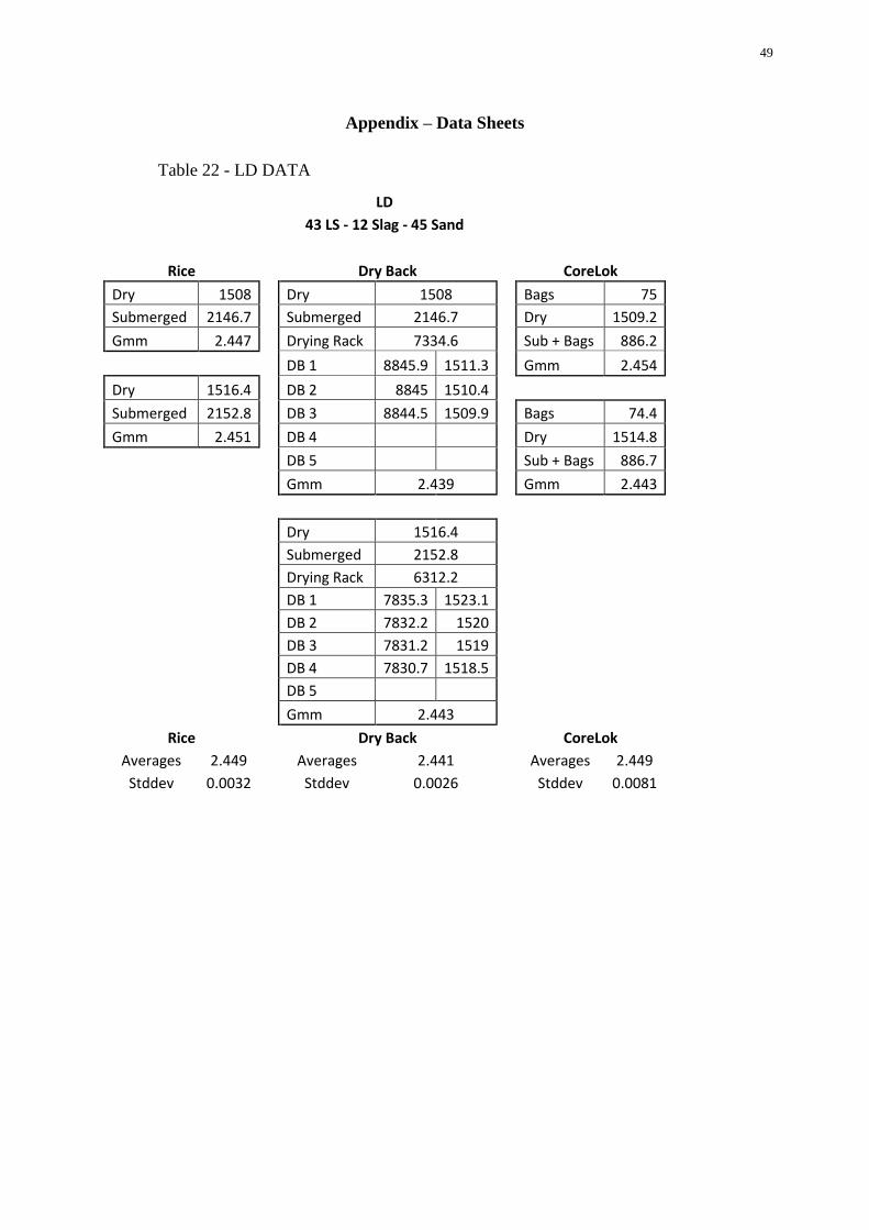
49

Appendix – Data Sheets

Table 22 - LD DATA

LD

43 LS - 12 Slag - 45 Sand

Rice Dry Back CoreLok

Dry 1508 Dry 1508 Bags 75

Submerged 2146.7 Submerged 2146.7 Dry 1509.2

Gmm 2.447 Drying Rack 7334.6 Sub + Bags 886.2

DB 1 8845.9 1511.3 Gmm 2.454

Dry 1516.4 DB 2 8845 1510.4

Submerged 2152.8 DB 3 8844.5 1509.9 Bags 74.4

Gmm 2.451 DB 4 Dry 1514.8

DB 5 Sub + Bags 886.7

Gmm 2.439 Gmm 2.443

Dry 1516.4

Submerged 2152.8

Drying Rack 6312.2

DB 1 7835.3 1523.1

DB 2 7832.2 1520

DB 3 7831.2 1519

DB 4 7830.7 1518.5

DB 5

Gmm 2.443


Averages 2.449 Averages 2.441 Averages 2.449

Stddev 0.0032 Stddev 0.0026 Stddev 0.0081

50

Table 23 - MD DATA

MD



Dry 1505.6 Dry 1505.6 Bags 74.3



DB 1 8849.4 1514.9 Gmm 2.439

Dry 1515.5 DB 2 8845.6 1511.1

Submerged 2149.3 DB 3 8844 1509.5 Bags 74.2

Gmm 2.440 DB 4 8843 1508.5 Dry 1497.2

DB 5 8842.7 1508.2 Sub + Bags 875.2

Gmm 2.428 Gmm 2.438

Dry 1515.5

Submerged 2149.3

Drying Rack 6313

DB 1 7842.2 1529.2

DB 2 7835.4 1522.4

DB 3 7833.8 1520.8

DB 4 7832.8 1519.8

DB 5 7832.3 1519.3

Gmm 2.425




51

Table 24 - HD DATA

HD



Dry 1511.2 Dry 1511.2 Bags 74.6

Submerged 2141 Submerged 2141 Dry 1492.7

Gmm 2.417 Drying Rack 7334.5 Sub + Bags 867

DB 1 8849.5 1515 Gmm 2.417

Dry 1514 DB 2 8848.5 1514

Submerged 2142.1 DB 3 Bags 74.2

Gmm 2.415 DB 4 Dry 1531.7


Gmm 2.406 Gmm 2.417

Dry 1514

Submerged 2142.1

Drying Rack 6312.2

DB 1 7832 1519.8

DB 2 7829 1516.8

DB 3 7828.5 1516.3

DB 4 -6312

DB 5

Gmm 2.406




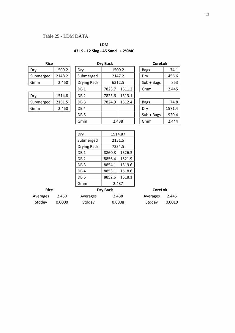
52

Table 25 - LDM DATA

LDM

43 LS - 12 Slag - 45 Sand + 2%MC


Dry 1509.2 Dry 1509.2 Bags 74.1



DB 1 7823.7 1511.2 Gmm 2.445

Dry 1514.8 DB 2 7825.6 1513.1


Gmm 2.450 DB 4 Dry 1571.4


Gmm 2.438 Gmm 2.444

Dry 1514.87

Submerged 2151.5

Drying Rack 7334.5

DB 1 8860.8 1526.3

DB 2 8856.4 1521.9

DB 3 8854.1 1519.6

DB 4 8853.1 1518.6

DB 5 8852.6 1518.1

Gmm 2.437




53

Table 26 - MDM DATA

MDM

28 LS - 27 Slag - 45 Sand +2% MC


Dry 1510.1 Dry 1510.1 Bags 74.5

Submerged 2146 Submerged 2146 Dry 1526


DB 1 8858.2 1523.7 Gmm 2.450

Dry 1509.6 DB 2 8851.7 1517.2

Submerged 2145 DB 3 8850 1515.5 Bags 74.8

Gmm 2.436 DB 4 8849.2 1514.7 Dry 1495.4

DB 5 8848.8 1514.3 Sub + Bags 874.4

Gmm 2.423 Gmm 2.440

Dry 1509.6

Submerged 2145

Drying Rack 6312.2

DB 1 7829.5 1517.3

DB 2 7826.6 1514.4

DB 3 7825.7 1513.5

DB 4 7825.4 1513.2

DB 5

Gmm 2.422




54

Table 27 - HDM DATA

HDM

13 LS - 42 Slag - 45 Sand +2% MC


Dry 1510.6 Dry 1510.6 Bags 74.1



DB 1 7837 1524.5 Gmm 2.423

Dry 1512.9 DB 2 7834.4 1521.9


Gmm 2.426 DB 4 7832.6 1520.1 Dry 1531.7

DB 5 7832.4 1519.9 Sub + Bags 892.1

Gmm 2.391 Gmm 2.425

Dry 1512.9

Submerged 2144.3

Drying Rack 7334.5

DB 1 8859.7 1525.2

DB 2 8857.4 1522.9

DB 3 8856.5 1522

DB 4 8855.7 1521.2

DB 5 8855.4 1520.9

Gmm 2.395




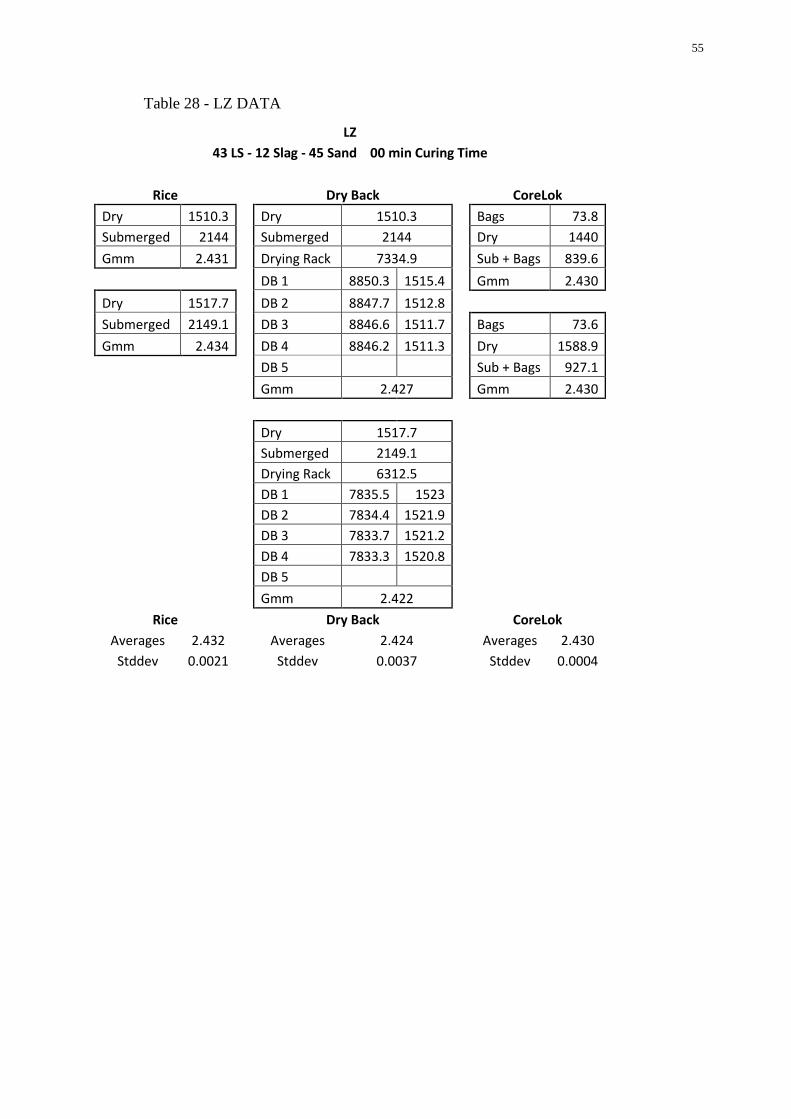
55

Table 28 - LZ DATA

LZ

43 LS - 12 Slag - 45 Sand 00 min Curing Time


Dry 1510.3 Dry 1510.3 Bags 73.8



DB 1 8850.3 1515.4 Gmm 2.430

Dry 1517.7 DB 2 8847.7 1512.8


Gmm 2.434 DB 4 8846.2 1511.3 Dry 1588.9


Gmm 2.427 Gmm 2.430

Dry 1517.7

Submerged 2149.1

Drying Rack 6312.5

DB 1 7835.5 1523

DB 2 7834.4 1521.9

DB 3 7833.7 1521.2

DB 4 7833.3 1520.8

DB 5

Gmm 2.422




56

Table 29 - MZ DATA

MZ



Dry 1510 Dry 1510 Bags 74.3



DB 1 8854.5 1519.9 Gmm 2.423

Dry 1510.9 DB 2 8853 1518.4


Gmm 2.426 DB 4 8851.4 1516.8 Dry 1512

DB 5 Sub + Bags 881

Gmm 2.401 Gmm 2.427

Dry 1510.9

Submerged 2143.1

Drying Rack 6312.2

DB 1 7831.6 1519.4

DB 2 7830.2 1518

DB 3 7829.5 1517.3

DB 4

DB 5

Gmm 2.401




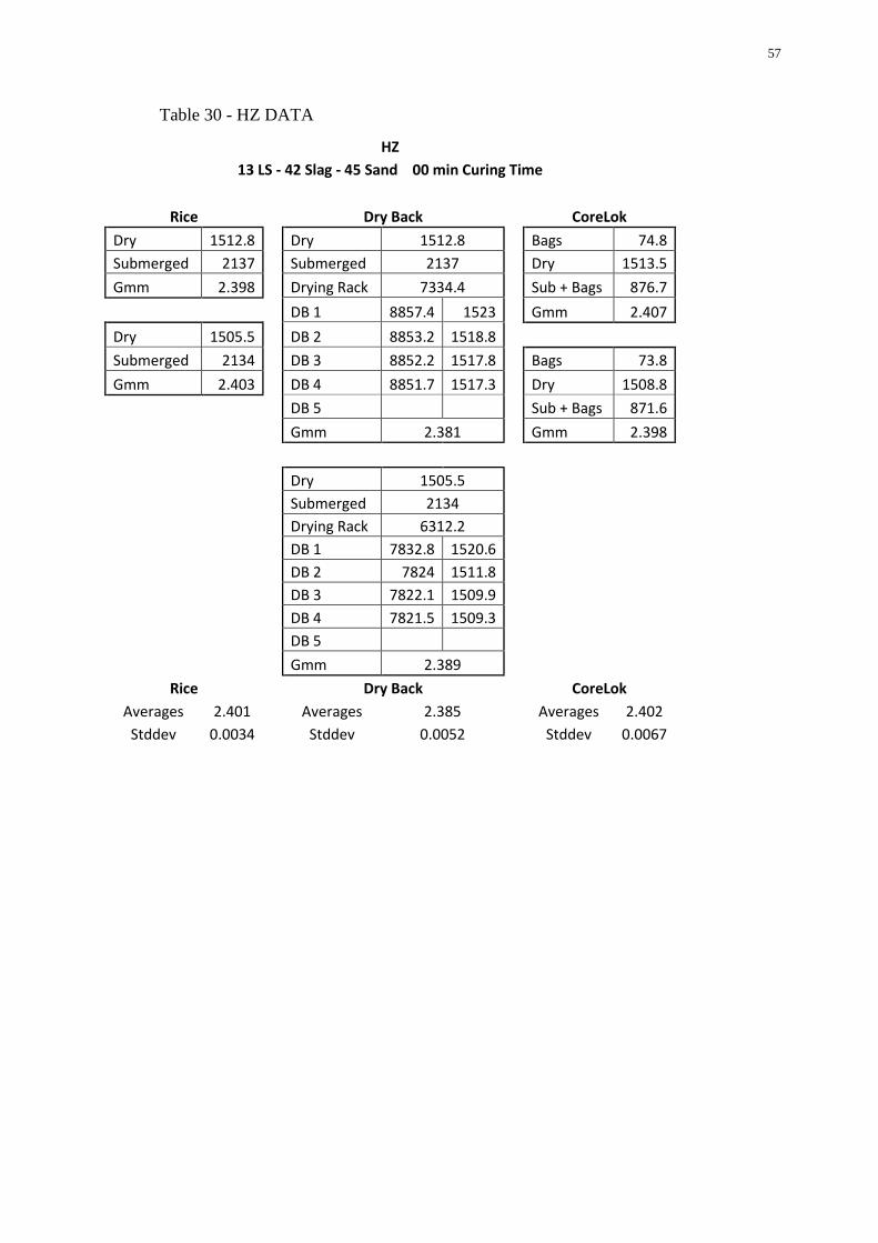
57

Table 30 - HZ DATA

HZ



Dry 1512.8 Dry 1512.8 Bags 74.8

Submerged 2137 Submerged 2137 Dry 1513.5


DB 1 8857.4 1523 Gmm 2.407

Dry 1505.5 DB 2 8853.2 1518.8

Submerged 2134 DB 3 8852.2 1517.8 Bags 73.8

Gmm 2.403 DB 4 8851.7 1517.3 Dry 1508.8


Gmm 2.381 Gmm 2.398

Dry 1505.5

Submerged 2134

Drying Rack 6312.2

DB 1 7832.8 1520.6

DB 2 7824 1511.8

DB 3 7822.1 1509.9

DB 4 7821.5 1509.3

DB 5

Gmm 2.389




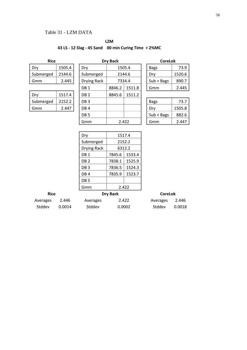
58

Table 31 - LZM DATA

LZM

43 LS - 12 Slag - 45 Sand 00 min Curing Time + 2%MC


Dry 1505.4 Dry 1505.4 Bags 73.9



DB 1 8846.2 1511.8 Gmm 2.445

Dry 1517.4 DB 2 8845.6 1511.2

Submerged 2152.2 DB 3 Bags 73.7

Gmm 2.447 DB 4 Dry 1505.8


Gmm 2.422 Gmm 2.447

Dry 1517.4

Submerged 2152.2

Drying Rack 6312.2

DB 1 7845.6 1533.4

DB 2 7838.1 1525.9

DB 3 7836.5 1524.3

DB 4 7835.9 1523.7

DB 5

Gmm 2.422




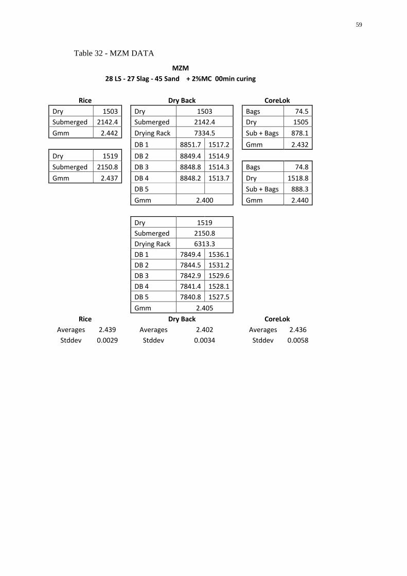
59

Table 32 - MZM DATA

MZM

28 LS - 27 Slag - 45 Sand + 2%MC 00min curing


Dry 1503 Dry 1503 Bags 74.5

Submerged 2142.4 Submerged 2142.4 Dry 1505


DB 1 8851.7 1517.2 Gmm 2.432

Dry 1519 DB 2 8849.4 1514.9


Gmm 2.437 DB 4 8848.2 1513.7 Dry 1518.8


Gmm 2.400 Gmm 2.440

Dry 1519

Submerged 2150.8

Drying Rack 6313.3

DB 1 7849.4 1536.1

DB 2 7844.5 1531.2

DB 3 7842.9 1529.6

DB 4 7841.4 1528.1

DB 5 7840.8 1527.5

Gmm 2.405




60

Table 33 - HZM DATA

HZM

13 LS - 42 Slag - 45 Sand + 2%MC 00min curing


Dry 1508.1 Dry 1508.1 Bags 74.4



DB 1 7843.8 1530.6 Gmm 2.429

Dry 1516.8 DB 2 7841.4 1528.2


Gmm 2.430 DB 4 7838.2 1525 Dry 1516

DB 5 7837.6 1524.4 Sub + Bags 885.3

Gmm 2.373 Gmm 2.434

Dry 1516.8

Submerged 2147.5

Drying Rack 7334.6

DB 1 8872.5 1537.9

DB 2 8870.6 1536

DB 3 8869.3 1534.7

DB 4 8868.2 1533.6

DB 5 8867.8 1533.2

Gmm 2.367




61

Table 34 - LP DATA

LP

43 LS - 12 Slag - 45 Sand +0.5% AC


Dry 1511.4 Dry 1511.4 Bags 73.8



DB 1 7835.8 1523.2 Gmm 2.435

Dry 1512.3 DB 2 7828.9 1516.3


Gmm 2.435 DB 4 7825.3 1512.7 Dry 1514.4

DB 5 7824.8 1512.2 Sub + Bags 882.3

Gmm 2.424 Gmm 2.426

Dry 1512.3

Submerged 2146.2

Drying Rack 7334.6

DB 1 8853.2 1518.6

DB 2 8851.5 1516.9

DB 3 8850.2 1515.6

DB 4 8849.5 1514.9

DB 5 8849.2 1514.6

Gmm 2.426




62

Table 35 - MP DATA

MP

9.5mm 28 LS - 27 Slag - 45 Sand +0.5% AC


Dry 1514.6 Dry 1514.6 Bags 74



DB 1 7831.1 1518.9 Gmm 2.419

Dry 1509.9 DB 2 7829.2 1517


Gmm 2.417 DB 4 Dry 1499.1

DB 5 Sub + Bags 870

Gmm 2.411 Gmm 2.414

Dry 1509.9

Submerged 2140.2

Drying Rack 7334.5

DB 1 8859.3 1524.8

DB 2 8850.2 1515.7

DB 3 8847.5 1513

DB 4 8846.2 1511.7

DB 5 8845.8 1511.3

Gmm 2.412




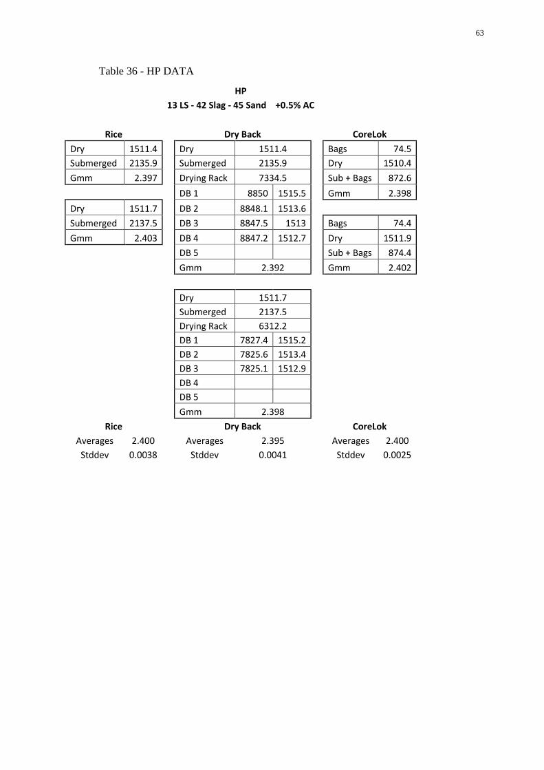
63

Table 36 - HP DATA

HP

13 LS - 42 Slag - 45 Sand +0.5% AC


Dry 1511.4 Dry 1511.4 Bags 74.5



DB 1 8850 1515.5 Gmm 2.398

Dry 1511.7 DB 2 8848.1 1513.6

Submerged 2137.5 DB 3 8847.5 1513 Bags 74.4

Gmm 2.403 DB 4 8847.2 1512.7 Dry 1511.9


Gmm 2.392 Gmm 2.402

Dry 1511.7

Submerged 2137.5

Drying Rack 6312.2

DB 1 7827.4 1515.2

DB 2 7825.6 1513.4

DB 3 7825.1 1512.9

DB 4

DB 5

Gmm 2.398




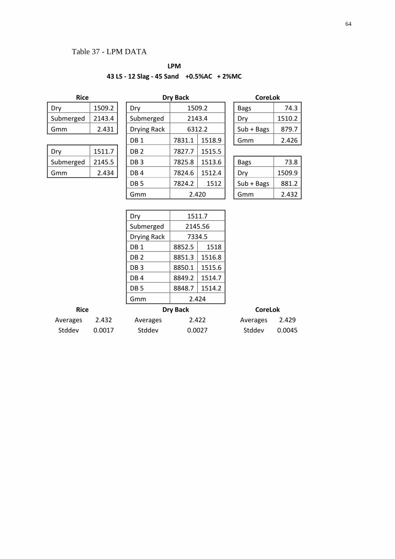
64

Table 37 - LPM DATA

LPM

43 LS - 12 Slag - 45 Sand +0.5%AC + 2%MC


Dry 1509.2 Dry 1509.2 Bags 74.3



DB 1 7831.1 1518.9 Gmm 2.426

Dry 1511.7 DB 2 7827.7 1515.5


Gmm 2.434 DB 4 7824.6 1512.4 Dry 1509.9

DB 5 7824.2 1512 Sub + Bags 881.2

Gmm 2.420 Gmm 2.432

Dry 1511.7

Submerged 2145.56

Drying Rack 7334.5

DB 1 8852.5 1518

DB 2 8851.3 1516.8

DB 3 8850.1 1515.6

DB 4 8849.2 1514.7

DB 5 8848.7 1514.2

Gmm 2.424




65

Table 38 - MPM DATA

MPM

28 LS - 27 Slag - 45 Sand +0.5% AC +2% MC


Dry 1510.7 Dry 1510.7 Bags 74.1



DB 1 8855.1 1520.7 Gmm 2.426

Dry 1509.5 DB 2 8852.1 1517.7


Gmm 2.428 DB 4 8850.1 1515.7 Dry 1511.8


Gmm 2.396 Gmm 2.426

Dry 1509.5

Submerged 2142.9

Drying Rack 6312.2

DB 1 7834.5 1522.3

DB 2 7830.8 1518.6

DB 3 7828.5 1516.3

DB 4 7827.5 1515.3

DB 5 7827.2 1515

Gmm 2.407




66

Table 39 - HPM DATA

HPM

13 LS - 42 Slag - 45 Sand + .5%AC + 2%MC


Dry 1513.1 Dry 1513.1 Bags 74.7



DB 1 8861 1525.6 Gmm 2.408

Dry 1507 DB 2 8858 1522.6


Gmm 2.406 DB 4 8856.3 1520.9 Dry 1507.5

DB 5 8855.9 1520.5 Sub + Bags 873.7

Gmm 2.372 Gmm 2.409

Dry 1507

Submerged 2135.6

Drying Rack 6312.2

DB 1 7835.9 1523.7

DB 2 7830.7 1518.5

DB 3 7828.3 1516.1

DB 4 7827.5 1515.3

DB 5 7827.1 1514.9

Gmm 2.376




Effects of Residual Moisture and Zero Conditioning Time … and Residual...Effects of Residual...

Documents

Transcript of Effects of Residual Moisture and Zero Conditioning Time … and Residual...Effects of Residual...