Effects of Foreign Aid on Public Expenditure of Developing Countries (2)

International Journal of Economics, Commerce and Management United Kingdom Vol. IV, Issue 8, August 2016
Licensed under Creative Common Page 508
http://ijecm.co.uk/ ISSN 2348 0386
EFFECTS OF RECURRENT PUBLIC EXPENDITURE
ON ECONOMIC GROWTH IN KENYA
Joseph Kivuva Mulinge
Department of Economics, Accounting and Finance, School of Business,
Jomo Kenyatta University of Agriculture and Technology, Kenya
Abstract
The purpose of this study was to find out the effect of recurrent public expenditure on economic
growth in Kenya from 1980-2014. The specific objectives of this study were to disaggregate
recurrent public expenditure into: government expenditure on social services, government
expenditure on general public administration, government expenditure on debt and to find out
the impact on economic growth in Kenya. This disaggregates were the independent variables
while real gross domestic product was the dependent variable. The study used time series data
covering the period 1980 – 2014. It employed Augmented Dickey Fuller test for unit root tests
before using autoregressive distributed lag approach to test cointegration. The study findings
indicated that; there was a long-term relationship between recurrent public expenditure and
economic growth in Kenya. Recurrent public expenditure on government social services and
government expenditure on debt showed a positive relationship towards growth while
government recurrent expenditure on administration showed a negative relationship. However,
government expenditure on debt and administration were statistically insignificant while
government recurrent expenditure on social services was statistically significant in driving
economic growth. The above finding should be used by the policymakers to ensure more funds
are allocated to recurrent budgets in the social sectors. The study also dispels the belief that
recurrent public expenditure components are always growth retarding in Kenya.
Keywords: Disaggregates, Economic Growth, Recurrent Public Expenditure, Social Sectors
International Journal of Economics, Commerce and Management, United Kingdom
Licensed under Creative Common Page 509
INTRODUCTION
Public expenditure can be broadly classified in terms of purpose as development and recurrent
expenditure. Development expenditure is expenditure on capital goods and projects that are
meant to increase the national output. Recurrent expenditure is a recurring spending on items
that are consumed only for a limited period of time. In the case of the government, recurrent
expenditure includes wages, salaries and expenditure on consumables - stationery, drugs for
health service, bandages and among others, Modebe (2012). Increasing recurrent expenditure
remains a challenge to many governments because the government is a major consumer of
goods and services in the economy. The relationship between public expenditure and economic
growth is a key subject of debate for economists and policymakers (Stiglitz, 2000).Economic
growth represents the expansion of a country‘s potential GDP or output. Economic growth is
important for jobs creation and poverty reduction in an economy. Consequently, the need to
stimulate economic growth through fiscal and monetary policies is, arguably, the best way to
break the vicious cycle of poverty in developing countries including Kenya. In this context,
understanding the impact of public expenditure becomes crucial if policymakers are to come up
with expenditure priorities that accelerate economic growth.
Government expenditure has been seen as a key driver of productivity in the economy
hence encouraging economic growth. In Kenya, Muthui et al (2013) finds results that show that
some components of public expenditure have positive and negative impacts on economic
growth. He specifically finds out that health, public order, security and education are positively
correlated to economic growth while defense expenditures are negatively correlated.
Controversially, Simiyu (2015) carried out a study to explain the relationship between public
expenditure and economic growth in Kenya using Vector Error Correction Model. In her study,
she found out that there was no causal relationship between public expenditure and economic
growth in Kenya. According to the Keynesian theories, government expenditure should promote
productivity but it has been an impediment just because of the way it is financed and allocated
among sectors. Public borrowing and imposition of taxes as a means of financing results to
crowding out of private investments and scaring away of potential investors respectively. This
study aims at investigating on the effect of recurrent public expenditure on economic growth in
Kenya and covers the period 1980-2014.
Government Expenditure in Kenya
During the initial years of independence, the movements of recurrent and development
expenditure were converging and these were the years Kenya recorded an upward growth
performance. For instance, there was an upward trend in development expenditure, reaching 36
© Mulinge
Licensed under Creative Common Page 510
percent of public expenditure in 1970 compared to 17 percent in 1963. This increase was
attributed to increase in the construction costs (Republic of Kenya, 2003). During this period, the
country was rebuilding and large amounts of money were spent on infrastructure and services.
There was a huge expenditure on electricity, roads, telecommunications and airport expansion.
A lot of money was also spent on resettlement, nationalization and agricultural development.
The proportion of development expenditure remained, on average 32 percent of total
expenditure from 1972-1979, but began to decline thereafter and stagnated at about 19 percent
of total government expenditure between 1982 -1996. A sharp decrease to less than 5 percent
between 1999 and 2002 was witnessed. The shrinking trends in development expenditure may
be blamed on the austerity measures by World Bank's in form of Structural Adjustment
Programmes (SAPs) or through International Monetary Fund (IMFs) stabilization programmes.
Since most recurrent expenditure is fixed the only leeway the government had in the wake of
these austerity measures was its development budget (M'Amanja and Morrissey, 2005).
Finally, development expenditure showed an upward trend between 2003 and 2007.
This was because of increased infrastructural expenditure in areas of roads, telecommunication,
health and education, rehabilitation of airport in Nairobi, Mombasa and Kisumu. Recurrent
expenditure showed a declining trend from about 80 percent of total expenditure in 1963, to
about67 percent in 1971. This is because most expenditure in education and health were in the
hands of the local authorities. From 1979 there was an upward trend in recurrent expenditure up
to 88 percent of expenditure in 1993, which later dropped to 77 percent of government
expenditure in 1996. This could be attributed to drought of 1980, compensation to Uganda
government for the assets it lost to Kenya due to collapse of East African Community, increased
expenditure on education since responsibility was transferred from local authority to central
government.
Education expenditure also increased due to expansion of educational physical facilities,
expanded curricular and increased demand for teachers wage bill as a result of implementation
of 8-4-4 system of education. The proportion of recurrent expenditure reached over 90 percent
between 1997-2000, due to large expenditure incurred to finance the general election of 1997
and higher salary rewards to teachers and civil servants. Thereafter it declined; reaching below
71 percent in 2007.The decline was as a result of government refocusing its expenditure in
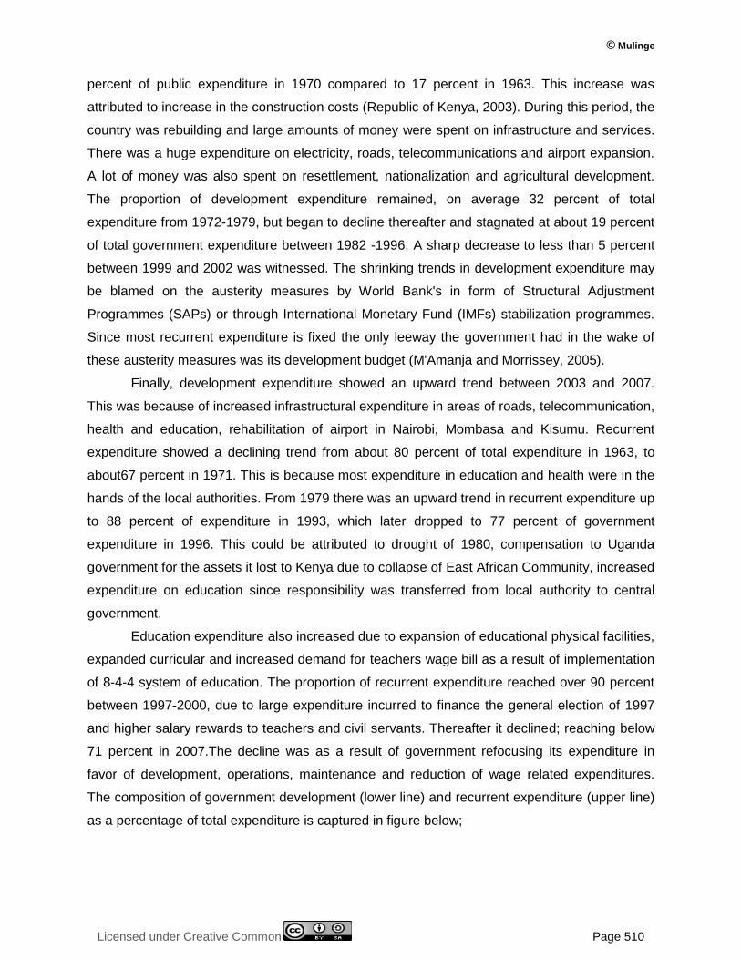
favor of development, operations, maintenance and reduction of wage related expenditures.
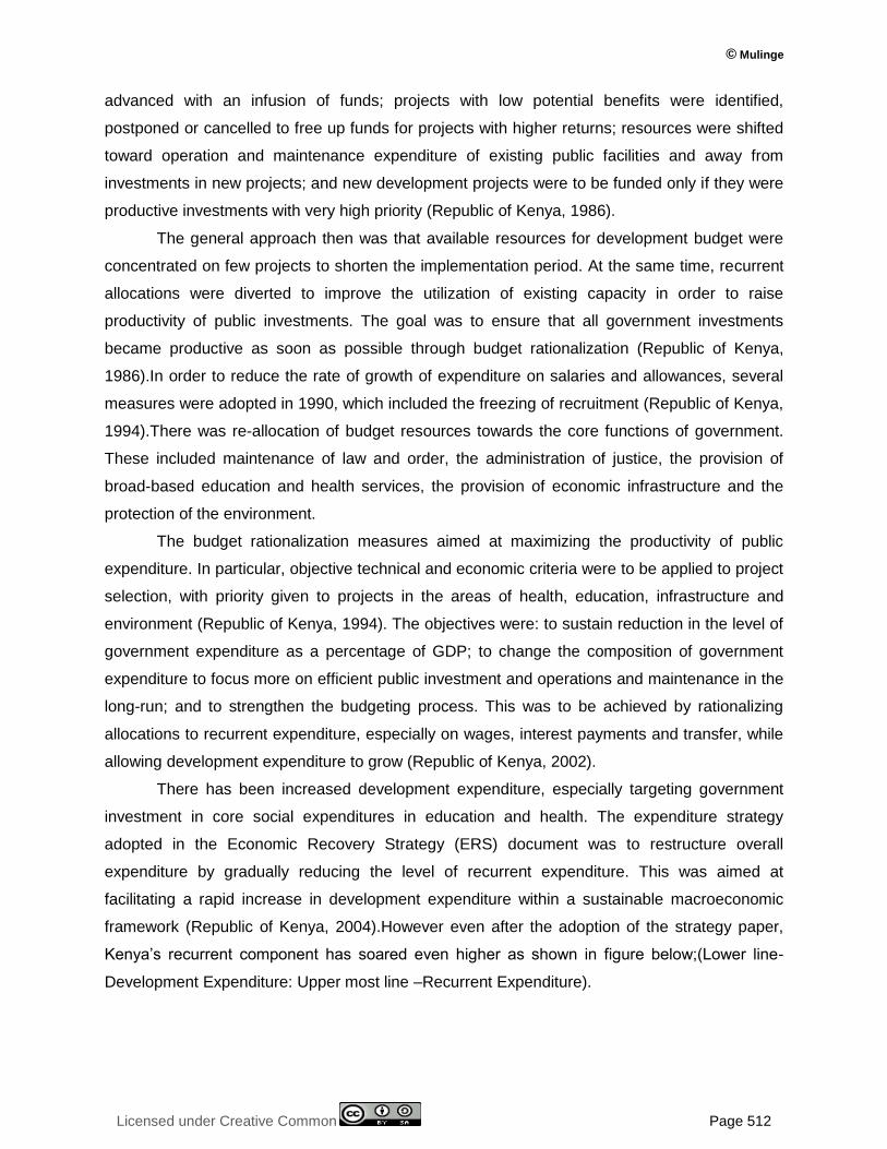
The composition of government development (lower line) and recurrent expenditure (upper line)
as a percentage of total expenditure is captured in figure below;
International Journal of Economics, Commerce and Management, United Kingdom
Licensed under Creative Common Page 511
Figure 1: Public expenditure in terms of development and recurrent expenditure in Kenya.
Source; Kenya National Bureau of Statistics, 2015
Recurrent Expenditure Reforms in Kenya
Since independence, various government expenditure reforms have been implemented to raise
and sustain the economic growth rate of the country. The public sector contributes to GDP
growth rate through provision of government services such as education, health and
administration, and productive activities in areas of agriculture, manufacturing, transport and
communication and trade. The government plays a leading role in determining the pattern of
financing its' operations through public sector reforms, which determine directly how much of the
country should borrow and how those resources should be allocated in order to enhance
economic growth. The main government expenditure strategy has been restructuring and
rationalizing overall expenditure.
During the planning periods 1979-2001, the government undertook rationalization of
government expenditure, with more resources being channeled to development and recurrent
non-wage operating and maintenance expenditure in order to stimulate economic growth
(Republic of Kenya, 1997).The central thrust of the policy was to rely on market forces to
mobilize resources for economic growth and development, with the role of government
increasingly confined to providing an effective regulatory framework and essential public
infrastructure and social services. The other major change in budget allocation involved a
concerted effort to make all government outlays more efficient and productive through budget
rationalization (Republic of Kenya, 1986). To achieve rationalization, the following measures
were taken: projects with potentially high productivity were identified and their completion was
© Mulinge
Licensed under Creative Common Page 512
advanced with an infusion of funds; projects with low potential benefits were identified,
postponed or cancelled to free up funds for projects with higher returns; resources were shifted
toward operation and maintenance expenditure of existing public facilities and away from
investments in new projects; and new development projects were to be funded only if they were
productive investments with very high priority (Republic of Kenya, 1986).
The general approach then was that available resources for development budget were
concentrated on few projects to shorten the implementation period. At the same time, recurrent
allocations were diverted to improve the utilization of existing capacity in order to raise
productivity of public investments. The goal was to ensure that all government investments
became productive as soon as possible through budget rationalization (Republic of Kenya,
1986).In order to reduce the rate of growth of expenditure on salaries and allowances, several
measures were adopted in 1990, which included the freezing of recruitment (Republic of Kenya,
1994).There was re-allocation of budget resources towards the core functions of government.
These included maintenance of law and order, the administration of justice, the provision of
broad-based education and health services, the provision of economic infrastructure and the
protection of the environment.
The budget rationalization measures aimed at maximizing the productivity of public
expenditure. In particular, objective technical and economic criteria were to be applied to project
selection, with priority given to projects in the areas of health, education, infrastructure and
environment (Republic of Kenya, 1994). The objectives were: to sustain reduction in the level of
government expenditure as a percentage of GDP; to change the composition of government
expenditure to focus more on efficient public investment and operations and maintenance in the
long-run; and to strengthen the budgeting process. This was to be achieved by rationalizing
allocations to recurrent expenditure, especially on wages, interest payments and transfer, while
allowing development expenditure to grow (Republic of Kenya, 2002).
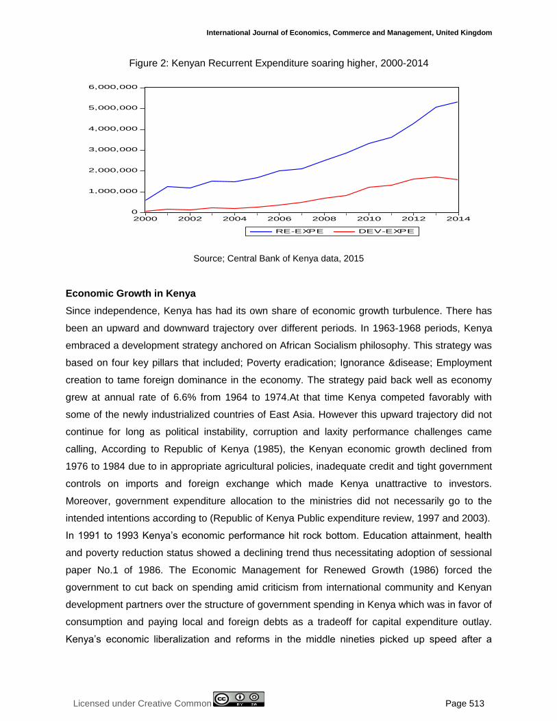
There has been increased development expenditure, especially targeting government
investment in core social expenditures in education and health. The expenditure strategy
adopted in the Economic Recovery Strategy (ERS) document was to restructure overall
expenditure by gradually reducing the level of recurrent expenditure. This was aimed at
facilitating a rapid increase in development expenditure within a sustainable macroeconomic
framework (Republic of Kenya, 2004).However even after the adoption of the strategy paper,
Kenya‘s recurrent component has soared even higher as shown in figure below;(Lower line-
Development Expenditure: Upper most line –Recurrent Expenditure).
International Journal of Economics, Commerce and Management, United Kingdom
Licensed under Creative Common Page 513
Figure 2: Kenyan Recurrent Expenditure soaring higher, 2000-2014
Source; Central Bank of Kenya data, 2015
Economic Growth in Kenya
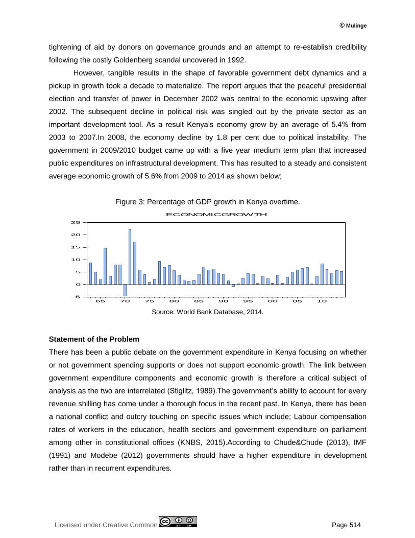
Since independence, Kenya has had its own share of economic growth turbulence. There has
been an upward and downward trajectory over different periods. In 1963-1968 periods, Kenya
embraced a development strategy anchored on African Socialism philosophy. This strategy was
based on four key pillars that included; Poverty eradication; Ignorance &disease; Employment
creation to tame foreign dominance in the economy. The strategy paid back well as economy
grew at annual rate of 6.6% from 1964 to 1974.At that time Kenya competed favorably with
some of the newly industrialized countries of East Asia. However this upward trajectory did not
continue for long as political instability, corruption and laxity performance challenges came
calling, According to Republic of Kenya (1985), the Kenyan economic growth declined from
1976 to 1984 due to in appropriate agricultural policies, inadequate credit and tight government
controls on imports and foreign exchange which made Kenya unattractive to investors.
Moreover, government expenditure allocation to the ministries did not necessarily go to the
intended intentions according to (Republic of Kenya Public expenditure review, 1997 and 2003).
In 1991 to 1993 Kenya‘s economic performance hit rock bottom. Education attainment, health
and poverty reduction status showed a declining trend thus necessitating adoption of sessional
paper No.1 of 1986. The Economic Management for Renewed Growth (1986) forced the
government to cut back on spending amid criticism from international community and Kenyan
development partners over the structure of government spending in Kenya which was in favor of
consumption and paying local and foreign debts as a tradeoff for capital expenditure outlay.
Kenya‘s economic liberalization and reforms in the middle nineties picked up speed after a
0
1,000,000
2,000,000
3,000,000
4,000,000
5,000,000
6,000,000
2000 2002 2004 2006 2008 2010 2012 2014
RE-EXPE DEV-EXPE
© Mulinge
Licensed under Creative Common Page 514
tightening of aid by donors on governance grounds and an attempt to re-establish credibility
following the costly Goldenberg scandal uncovered in 1992.
However, tangible results in the shape of favorable government debt dynamics and a
pickup in growth took a decade to materialize. The report argues that the peaceful presidential
election and transfer of power in December 2002 was central to the economic upswing after
2002. The subsequent decline in political risk was singled out by the private sector as an
important development tool. As a result Kenya‘s economy grew by an average of 5.4% from
2003 to 2007.In 2008, the economy decline by 1.8 per cent due to political instability. The
government in 2009/2010 budget came up with a five year medium term plan that increased
public expenditures on infrastructural development. This has resulted to a steady and consistent
average economic growth of 5.6% from 2009 to 2014 as shown below;
Figure 3: Percentage of GDP growth in Kenya overtime.
Source: World Bank Database, 2014.
Statement of the Problem
There has been a public debate on the government expenditure in Kenya focusing on whether
or not government spending supports or does not support economic growth. The link between
government expenditure components and economic growth is therefore a critical subject of
analysis as the two are interrelated (Stiglitz, 1989).The government‘s ability to account for every
revenue shilling has come under a thorough focus in the recent past. In Kenya, there has been
a national conflict and outcry touching on specific issues which include; Labour compensation
rates of workers in the education, health sectors and government expenditure on parliament
among other in constitutional offices (KNBS, 2015).According to Chude&Chude (2013), IMF
(1991) and Modebe (2012) governments should have a higher expenditure in development
rather than in recurrent expenditures.
-5
0
5
10
15
20
25
65 70 75 80 85 90 95 00 05 10
ECONOMICGROWTH
International Journal of Economics, Commerce and Management, United Kingdom
Licensed under Creative Common Page 515
However, this rarely happens because in developing and middle developed countries
governments grapple with many challenges (huge wage bill, unemployment, huge external
borrowing for infrastructural development, corruption and political instabilities). According to
Lotto (2011) and Devarajan &Vinay (1993) some aspects of recurrent sectoral expenditure have
a positive effect and negative effects on economic growth in Nigeria. There are various studies
that have been done in Kenya about the impact of government expenditure on economic
growth, Muthui et al (2013); Simiyu (2015); among others. However, these studies have been
sectoral based cutting across development and recurrent expenditures. This study therefore
seeks to fill the gap by establishing the effects of recurrent expenditure on economic growth in
Kenya.
Objectives of the Study
The general objective was to determine the effect of recurrent public expenditure components
on economic growth in Kenya.
The specific objective is to;
i. Determine the effect of government recurrent expenditure on social services on
economic growth.
ii. Find out the relationship between government general public administration and
economic growth.
iii. Investigate the impact of government expenditure on debt interest payments on
economic growth.
Significance of the study
This study will help policymakers in Kenya and elsewhere in coming up with prudent measures
by allocating a huge chunk of recurrent expenditures to recurrent components that drive
economic growth. It will also be useful for other developing countries especially in Sub-Saharan
Africa which share similar characteristics with Kenya.
Scope of Study
The study covered Kenyan government recurrent expenditures on the above outlined
components from 1980-2014. This is because there were huge structural adjustments in the
1980s, 1990s and after 2011 due to the promulgation of the new constitution.
© Mulinge
Licensed under Creative Common Page 516
Limitations of Study
The study specifically focused on the government expenditure going to various recurrent
components of the economy but does not intend to look into entire public expenditure
components.
LITERATURE REVIEW
Theoretical Literature
The theories that explain government expenditure are outlined below;
Wagner Theory of Organic State
Among the pioneer literatures on public expenditure was one German economist called
Wagner. The literature opines that growth of public spending was a natural consequence of
economic growth. Specifically, Wagner law viewed public expenditure as a behavioral variable
that positively responded to the dictates of a growing economy, Wagner (1977). The hypothesis
tries to find either a positive relationship between government spending and income or a
unidirectional causality running from government spending to economic growth. The Wagner
law is admired because it in many ways attempts to explain public expenditure and economic
growth. The law is faulted because of its inherent assumption of viewing the state as separate
entity capable of making its decisions ignoring the constituent‘s populace who in actual fact can
decide against the dictates of the Wagner Law.
Musgrave Rostow’s Theory
This theory asserts that in early stages of economic growth, public expenditure in the economy
should be encouraged, Musgrave (1959). The theory further states during the early stages of
growth there exists market failures and hence there should be robust government involvement
to deal with these market failures. This theory is faulted because it ignores the contribution to
development by the private sector by assuming the government expenditure is the only driver of
economic growth.
Keynesian Theory
The Keynesian model indicates that during recession a policy of budgetary expansion should be
undertaken to increase the aggregate demand in the economy thus boosting the Gross
Domestic Product (GDP). This is with a view that increases in government spending leads to
increased employment in public sector and firms in the private sector. When employment rises;
then income and profits of the firms increase, and this results in firms hiring more workers to
International Journal of Economics, Commerce and Management, United Kingdom
Licensed under Creative Common Page 517
produce the goods and services needed by the government. In consonance to the above, the
work of Barro has stipulated a new perspective in which the investigation of the impact of fiscal
budgetary expansion through public expenditure can enhance output growth. The authors
employed a Cobb Douglas model and found that government activity influences the direction of
economic growth (Barro& Sula-i-Martin,1992).However; one of the greatest limitations of
Keynesian theory is that it fails to adequately consider the problem of inflation which might be
brought about by the increase in government spending.
The Peacock and Wiseman Theory This theory was advanced by peacock and Wiseman in a study of public expenditure in the UK
for the period 1890 – 1955. It‘s based on premise that, the populace is naturally tax averse while
the government on the other hand has an inherent appetite for expenditure. During times of
shocks like calamities and war, the government would expeditiously increase the public
expenditure, this necessitates moving taxes upwards, the researchers argued that the populace
(tax payers) would allow and condone such an increase in tax. This scenario is referred to as
displacement effect, though it‘s meant to be a short term phenomenon it normally assume a
long term trend (Wiseman and Peacock, 1961).This can attempt to explain how government
expenditure in Kenya has taken unrelenting upward trajectory. Every time Kenya has
experienced shocks like, 1984 famine, resettlement of internally displaced persons and upsizing
of the government structure to accommodate the many ministries intended to serve the citizens,
the taxes intensify and scope matched in tandem with the public expenditure. One of the
shortcomings of this theory is that it sidelines the fact that government can finance an upward
displacement in public expenditure using other sources of finance such as donor funds, external
borrowing or even sale of government fixed asset and this needless to say may not affect taxes
in an upward trend.
Ernst Engel’s Theory of Public Expenditure
Ernst Engel was also a German economist writing almost the same time as Adolph Wagner in
the 19th century. Engel pointed out over a century ago that the composition of the consumer
budget changes as family income increases, Zimmerman (1932). A smaller share comes to be
spent on certain goods such as work clothing and a larger share on others, such as for coats,
expensive jewelries etc. As average income increase, smaller charges in the consumption
pattern for the economy may occur. At the earlier stages of national development, there is need
for overhead capital such as roads, harbors, power installations, pipe-borne water etc. But as
the economy developed, one would expect the public share in capital formation to decline over
© Mulinge
Licensed under Creative Common Page 518
time. Individual expenditure pattern is thus compared to national expenditure and Engel finding
is referred to as the declining portion of outlays on foods.
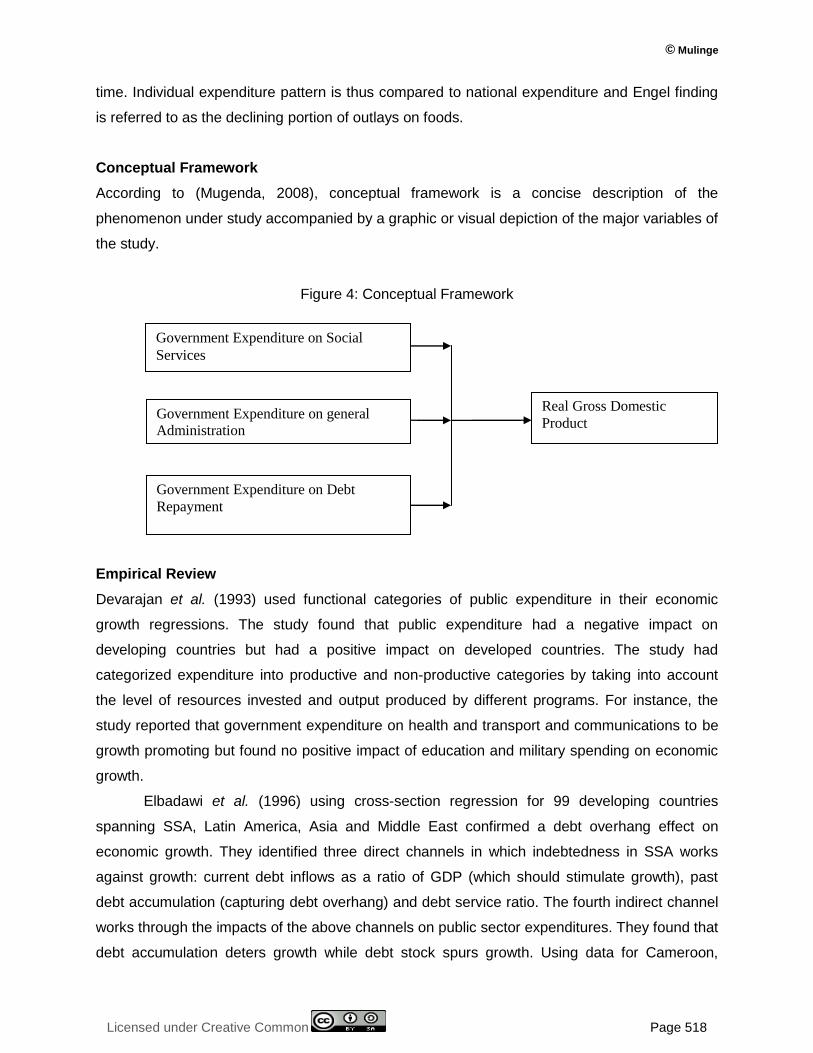
Conceptual Framework
According to (Mugenda, 2008), conceptual framework is a concise description of the
phenomenon under study accompanied by a graphic or visual depiction of the major variables of
the study.
Figure 4: Conceptual Framework
Empirical Review
Devarajan et al. (1993) used functional categories of public expenditure in their economic
growth regressions. The study found that public expenditure had a negative impact on
developing countries but had a positive impact on developed countries. The study had
categorized expenditure into productive and non-productive categories by taking into account
the level of resources invested and output produced by different programs. For instance, the
study reported that government expenditure on health and transport and communications to be
growth promoting but found no positive impact of education and military spending on economic
growth.
Elbadawi et al. (1996) using cross-section regression for 99 developing countries
spanning SSA, Latin America, Asia and Middle East confirmed a debt overhang effect on
economic growth. They identified three direct channels in which indebtedness in SSA works
against growth: current debt inflows as a ratio of GDP (which should stimulate growth), past
debt accumulation (capturing debt overhang) and debt service ratio. The fourth indirect channel
works through the impacts of the above channels on public sector expenditures. They found that
debt accumulation deters growth while debt stock spurs growth. Using data for Cameroon,
Government Expenditure on Social
Services
Government Expenditure on general
Administration
Government Expenditure on Debt
Repayment
Real Gross Domestic
Product

International Journal of Economics, Commerce and Management, United Kingdom
Licensed under Creative Common Page 519
Mbanga and Sikod (2001) found that there exist a debt overhang and crowding-out effects on
private and public investments, respectively. Other studies that have found a negative effect of
external debt on growth include Degefe (1992). Some studies simply use simulation analysis to
show the impact of the debt burden indicators on economic growth under different scenarios
(Ajayi (1991); Osei(1995).
Kuştepeli, (2005) carried out a study to determine how government size affected the
economic growth by focusing on OECD countries in the period 1970 – 1999. The study using
panel data alluded to the fact that the government size had a negative and statistically
significant impact on economic growth. The only countries which did not fall under the above
conclusion were United States of America, Sweden and Norway with their coefficients turning
out to be statistically insignificant.
M‘Amanja and Morrissey (2005) in their paper entitled ―Fiscal Policy and Economic
Growth in Kenya‖ found that unproductive expenditure and non-distortionary tax revenue to be
neutral to growth as predicted by economic theory and productive expenditure has strong
adverse effect on growth whilst there was no evidence of distortionary effects on growth of
distortionary taxes.
Jerono (2009) conducted a study on the impact of government spending on economic
growth in Kenya and found that though expenditure on education had a positive relationship
with economic growth; it does not spur any significant change to growth. Given the reason that
the expansion of education is higher than that of job growth in Kenya and there are relatively
few job opportunities outside government for secondary and university graduates hence the
education system has been blamed for producing surplus graduates, and long waits for
government jobs. The study also asserted that a mere expenditure growth does not necessarily
spur growth; growth on the GDP was dependent on other factor too such as political will
efficiency and also prioritization on the key components of the economy.
Maingi (2011) while conducting study on the impact of government expenditure on economic
growth in Kenya reported that improved government expenditure on areas such as physical
infrastructure development and in education enhance economic growth while areas such as
foreign debts servicing, government consumption and expenditure on public order and security,
salaries and allowances were growth retarding.
Loto (2011) investigated the growth effect of government expenditure on economic
growth in Nigeria over the period of 1980 and 2008, with a particular focus on sectoral
expenditures. His study was based on the use of five key sectors; security, health, education,
transportation and communication and agriculture. His results indicated that in the short-run,
expenditure on agriculture is negatively related to economic growth. The impact of the
© Mulinge
Licensed under Creative Common Page 520
expenditure on the educational sector was also observed to be negative and not significant. The
impact of expenditure on health was found to be positively related to economic growth. Finally,
the results showed that while the expenditure on national security transportation and
communication was positively related to economic growth, their impact was not statistically
significant.
Saheed (2012) examined the impact of government capital expenditure on exchange
rate in Nigeria, using disaggregated approach. The findings of the study indicated that the
government‘s capital expenditure, especially government spending on social and community
services has a statistically significant impact on exchange rate in Nigeria, while capital
expenditures on administration, economic services and transfer are not statistically significant in
respect to their impact on exchange rate. In studying the effect of the composition of public
expenditure on growth in Nigeria using the vector error correction approach (VEC),
Onotaniyohwo et al (2012) found that the expenditure on transfers had a significant but negative
impact on growth while the expenditure on economic and social-community services had a
significant and positive impact on growth.
Muthui et al (2013), while investigating the impact of government expenditure
components: (education, infrastructure, health, defense and public order and security)on
economic growth in Kenya found out that government expenditure on education is positively
related to economic growth it does and it does not spur any significant change to growth. The
study also found out increased expenditure on improving health might be justified purely on the
grounds of its impact on labor productivity. This supports the case for investments in health as a
form of human capital. To reduce the huge budget outlay for importing medicine and drugs, this
study recommended for government to support research and development in this sector locally.
Critique of the Existing Literature Relevant to the Study
From the literature reviewed so far, it may be observed that while a lot of research has been
carried out on the impact of government expenditure on economic growth in Kenya, no attempt
has so far been made to study the growth impact of the recurrent public expenditure on the
economic growth. This is supported by the fact that most governments believe that recurrent
expenditures are bad for the economy. The policy makers have been in verge of taming
recurrent public expenditures at whatever cost.
However, in this study an attempt is made to establish the effect of recurrent public
expenditure components on economic growth in Kenya.
International Journal of Economics, Commerce and Management, United Kingdom
Licensed under Creative Common Page 521
Summary of Literature
The first part of the literature review highlighted basic theories that have been used to support
the effects of government expenditure on economic growth. There are five theories that have
been discussed; But three form a key interest for our study which include: the Keynesian theory,
Wagner‘s theory of increasing state activities, and Musgrave theory of public expenditure
growth. From these theories, we realize there are different views of the effect of government
spending on economic growth. According to Keynesian view, government could reverse
economic downturns by borrowing money from the private sector and then returning the money
to the private sector through various spending programs. High levels of government
consumption are likely to increase employment, profitability and investment via multiplier effects
on aggregate demand. Thus, government expenditure, even of a recurrent nature, can
contribute positively to economic growth. Wagner‘s theory on the other hand emphasizes that
increase in public demand leads to proportional increase in national income.
Musgrave theory on the other hand observes that at the high levels of per capita income,
typical of developed economics, the rate of public sector growth tends to fall as the more basic
wants are being satisfied. From the empirical literature review, various findings have also
contradicted each other. Some of them relate economic growth increase to government
expenditure increase while others attribute negative economic growth to government
expenditure as well. It is worth noting that the differences in the outcome of these findings could
be as a result of the different exploratory variables used in different combinations and different
contexts. But what remains for sure is that government expenditure has a great impact on the
economic growth of a country.
Research Gap
As revealed from the literature reviewed so far, different exploratory variables lead to different
outcomes in the study of economic growth and public expenditure. Although these studies were
done in different African contexts, none of those reviewed was based on Kenyan context as
similar studies done in Kenya do not disaggregate recurrent public expenditure into specific
components. These studies hardly give policy recommendations and implications of recurrent
public expenditure on economic growth. This study seeks to fill this gap by providing necessary
literature, disaggregating recurrent public expenditure into major specific components and
finding out how each component impacts economic growth. This study becomes even more
useful because the researcher provided policy recommendations at the end of the study that
can be adopted by the current government.
© Mulinge
Licensed under Creative Common Page 522
METHODOLOGY
Research Design
Descriptive studies are usually the best methods for collecting information that will demonstrate
relationships and describe the world as it exists. These types of studies are often done before
an experiment to know what specific things to manipulate and include in an experiment. Elahi &
Dehdashti, (2011) suggest that descriptive studies can answer questions such as ―what is‖ or
―what was.‖ Experiments can typically answer ―why‖ or ―how.‖ The focus of this study was to
establish the relationships between variables of interest and the causal effects. It is important to
note that just because variables are related, does not necessarily mean that one directly causes
the other. This study was descriptive in nature and involved quantitative analysis of data.
Target Population
The study focused on time series data for three economic variables for the period from 1980 to
2014. This study concentrated on the following variables; dependent variable, economic growth
(measured by the Real GDP) and independent variables namely government expenditure on
public administration, government expenditure on debt, and government expenditure on social
services. The choice is also for the avoidance of structural breaks problems. The data will
investigate the whole study area and for that reason there will be no sampling undertaken.
Data Collection Instruments
According to (Ngechu, 2004), there are many methods of data collection. The choice of a tool
and instrument depends mainly on the attributes of the subjects, research topic, problem
question, objectives, design, expected data and results. This is because each tool and
instrument collects specific data. This study used secondary data which was collected from the
Central Bank of Kenya website, Kenya National Bureau of Statistics website, and the Treasury
publications.
Variables Description and Justification
Government Expenditure on Social services
Consists of all recurrent health and education expenditure .This is total expenditure on
education made by the central government for pre-primary through tertiary education. It also
means expenditure made by the central government for hospitals, clinics, and public health
affairs and services for medical, dental and paramedical practitioners; for medication, medical
equipment and appliances; for applied research and experimental development.
International Journal of Economics, Commerce and Management, United Kingdom
Licensed under Creative Common Page 523
Government Expenditure on General Public Administration
This is the government expenditure on the national assembly, senate, judiciary and
constitutional commissions. These are recurring expenditures on salaries and sitting allowances
of members of parliament, senate, judiciary and constitutional commissions. The persistent
public outcry in recent times over the perceived unnecessarily large expenditure on the Kenyan
public administration, and the question of the extent of their contribution to the overall growth of
the nation is worrisome. The importance of expenditure on the constitutional pillars is derived
from the role of the general administration in the creation of an enabling environment for the
growth of economic activities through the promulgation, review and amendment of laws,
interpreting the laws, evaluation and approval of national budgets, as well as their oversight
functions which has to do with the power of the national assembly to review, monitor and
supervise agencies, programmes, activities and policy implementation of the executive arm of
government, Ndoma.,E.(2012).
Government Expenditure on Debt Repayments
This is the government expenditure on both external and internal debt repayments. External
debt constitutes all money borrowed outside the country while the internal debt includes all
money that is borrowed within the country. Kenya‘s external debt indicators-debt-to-GDP ratio
and debt-to exports ratio—have risen from an average of 38.5 per cent and 121.1 per cent for
the 1970-80 period to 89.2 per cent and 268.2 per cent for 1991-99 period, respectively.
Meanwhile, there have been significant net outflows since 1991 to service the debt obligations.
There are various questions that form an area of interest in this study; Is Kenya paying out more
funds than it receives, thereby reducing domestic resources available for development? Are the
amounts of money borrowed put into growth promoting or retarding activities? Although
domestic debt constitutes less than a third of the total formal debt, it is almost ten times as
expensive as external debt (GoK2014).
Data Analysis and Presentation
Before subjecting the data to a regression analysis, a descriptive statistics test has to be
conducted to provide a general view of the distribution and behavior of the variables in use. This
entails showing trends of the variables in form of tables, graphs, and charts. Residual test for
normality of the data series will be conducted and the Jacque Bera coefficient and its p-value
will be observed for significance.
From the above analysis and for obvious statistical reasons, the logs (L) of all the
variables will be calculated. The regression equation will be as follows;
© Mulinge
Licensed under Creative Common Page 524
LRGDP = tLGEDLGEALGES 3210 …………………………………………. (1)
RGDP-Real gross domestic product 0 -constant term
GES- Government expenditure on social services t-Error term
GEA- Government expenditure on general administration
GED- Government expenditure on debt
Stationarity Test/Stability test
This is done to ensure that variables are stationary and that shocks are only temporary and will
dissipate and revert to their long-run mean (Maysami, Howe, & Hamzah, 2004). In time series
analysis, the Ordinary Least Squares regression results might provide a spurious regression if
the data series are non-stationary. Thus, the data series must obey the time series properties
i.e. the time series data should be stationary, meaning that, the mean and variance should be
constant over time and the value of covariance between two time periods depends only on the
distance between the two time period and not the actual time at which the covariance is
computed.
For solution to the research question to be feasible, a stability analysis was carried out
(Dimitrova, 2005). The augmented Dickey Fuller test was used to establish whether the data
was stationary or not and also to determine the order of integration of the variables. It involved
the following equations.
∆𝐺𝐷𝑃 = 𝑎0 + 𝛽𝑡 + θyt − 1 + ρ∆GDPt − i + et 𝑚𝑡=1 (For levels) ……………............ (2)
∆∆𝐺𝐷𝑃 = 𝑎0 + 𝛽𝑡 + θ∆yt − 1 + ρ∆∆GDPt − i + et 𝑚𝑡=1 (For first differences).......... (3)
There are cases where ADF doesn‘t have a drift and a trend but the example has both a drift
(intercept) and a trend. Where 𝑎0 is a drift, m is the number of lags and e is the error term and t
is trend.
The null hypothesis will be HO: (𝑎0, 𝛽, 𝜃) = (𝑎0, 0, 1) (No-Stationarity)
The alternative hypothesis H1: (𝑎0, 𝛽, 𝜃) ≠ (𝑎0, 0, 1) (Stationarity)
If the test reveals that null hypothesis should be rejected than the variable will be said to be
stationary.
Cointegration Test
The study used bound testing technique which is based on three validations to test for
cointegration. First, Pesaran et al. (2001) advocated the use of the ARDL model for the
estimation of level relationships because the model suggests that once the order of the ARDL
has been recognised, the relationship can be estimated by OLS. Second, the bounds test allows
International Journal of Economics, Commerce and Management, United Kingdom
Licensed under Creative Common Page 525
a mixture of I(1) and I(0) variables as regressors, that is, the order of integration of appropriate
variables may not necessarily be the same. Therefore, the ARDL technique has the advantage
of not requiring a specific identification of the order of the underlying data. Third, this technique
is suitable for small or finite sample size (Pesaran et al., 2001).
Following Pesaran et al. (2001), we assemble the vector auto regression (VAR) of order p,
denoted VAR (p), for the following growth function:
tit
p
i
it zZ
1 ............................................................................................... (4)
Where z t is the vector of both x t and y t , where y t is the dependent variable defined as
economic growth (RGDP), tx is the vector matrix which represents a set of explanatory
variables. According to Pesaran et al. (2001), tymust be I(1) variable, but the regressor tx
can
be either I(0) or I(1). We further developed a vector autoregression model (VAR) as follows:
tit
p
i
tit
ip
i
ttt xyztz
1
11
1
..................................................................(5)
where is the first-difference operator. The long-run multiplier matrix as:
XXXY
YXYY
The diagonal elements of the matrix are unrestricted, so the selected series can be either I (0)
or I(1). If 0YY , then Y is I(1). In contrast, if 0YY , then Y is I (0).
The VECM procedures described above are imperative in the testing of at most one
cointegrating vector between dependent variable tyand a set of regressors tx
. To derive model,
we followed the postulations made by Pesaran et al. (2001) in case III, that is, unrestricted
intercepts and no trends. After imposing the restrictions 0,0 YY and
)6......(..........)()()()(
)()()()()(
t0
7
0
7
0
5
1
4
131312110
it
S
i
it
r
i
it
q
i
it
p
i
ttttt
LGEALGEDLGESLRGDP
LGEALGEDLGESLRGDPLRGDP
Where u t is a white-noise disturbance term;
RGDP = Logarithm of Real Gross Domestic Product
LGES = Logarithm of government expenditure on social services
LGED = Logarithm of government expenditure on debt
LGEA =Logarithm of government expenditure on general public administration
© Mulinge
Licensed under Creative Common Page 526
Equation (6) also can be viewed as an ARDL of order (p, q, r, s). Equation 6 indicates that
economic growth tends to be influenced and explained by its past values. The structural lags
are established by using minimum Akaike‘s information criteria (AIC).The short-run effects are
captured by the coefficients of the first-differenced variables in equation 6.
Granger Casuality Test
The Granger Casuality test determines the casual relationship between GDP growth and public
expenditure components. The Granger method sought to explain how much of a variable X
(public expenditure components) can be explained by its own past values and whether adding
lagged values of another variable Y (GDP growth) can explain better. It involves estimation of
the following equations:
Yt = 𝛼0 + 𝛼1Y𝑡−1 + βjX𝑡−1 + ε1nj=1
𝑛𝑖=1 ………………………………………………...(7)
Xt = 𝛼0 + 𝛼 ∋1 Y𝑡−1 + δjX𝑡−1 + ε2mj=1
𝑚𝑖=1 ……………………………………………..(8)
In the model, "t" denotes time periods and ε is a white noise error term. The constant parameter
𝛼0 denotes constant growth rate of Y in equation (7) and for X in equation (8). The trend is
interpreted as general movements of cointegration between X and Y that follows the unit root
process.
Model Specification
This study aimed at establishing the dynamic properties of the relationship between government
spending and RGDP in Kenya over the years (1980-2014). The functional form, on which our
model was based, employed a multiple regression equation in the analysis of this work. In an
attempt to capture our essence of this study, and based on previous studies the Real Gross
Domestic Product (RGDP),Government Expenditure on social services(GES); Government
Expenditure on general public administration (GEA) and Government expenditure on debt
(GED) were used to formulate our model.
The following model which represents linearity is formulated as follows:
Y = 𝜷𝟎+ 𝜷𝟏𝑿𝟏 + 𝜷𝟐𝑿𝟐 + 𝜷𝟑𝑿𝟑+ 𝟏 ………………………………………………….. (9)
Where: Y: represents the economic growth measured by per real gross domestic product.
X1: Government Expenditure on Social services.
X2: Government Expenditure on general public administration.
X3: Government Expenditure on Debt.
International Journal of Economics, Commerce and Management, United Kingdom
Licensed under Creative Common Page 527
𝛽1, 𝛽2 and 𝛽3: represents the coefficients values of the three independent variables,
respectively.
𝛽0: represents the constant term.
1: Represents the error term
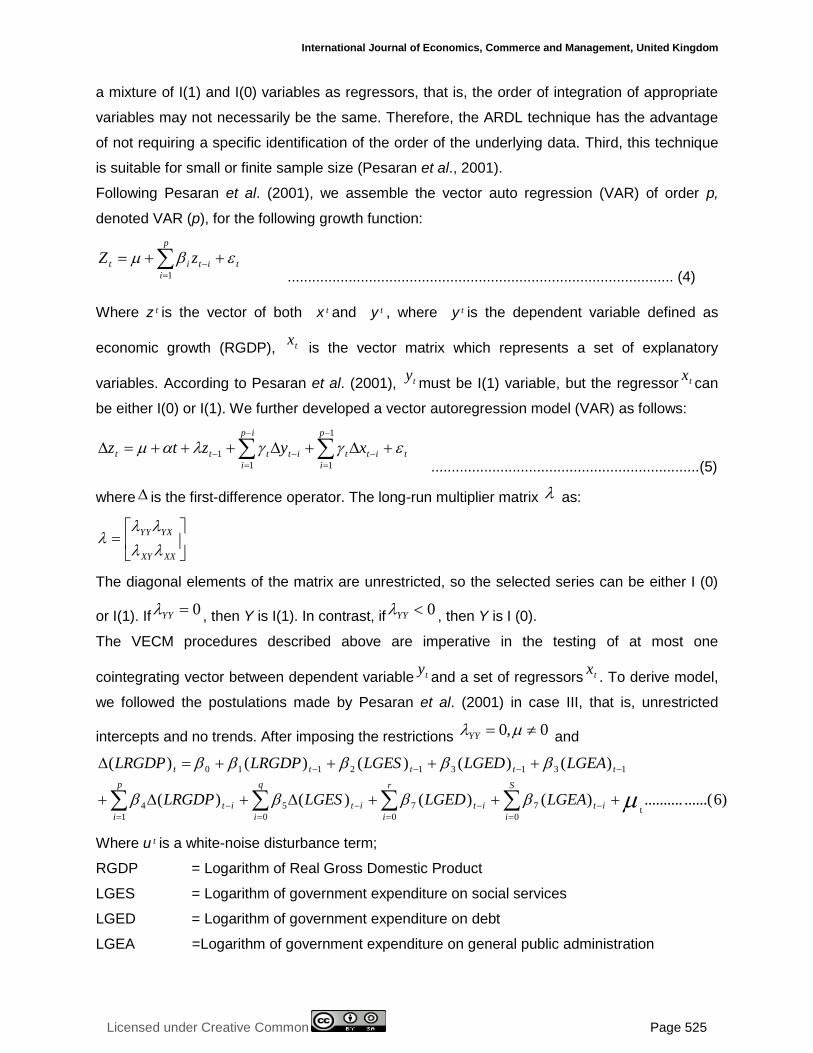
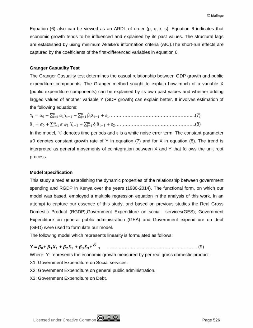
RESEARCH FINDINGS & DISCUSSION
For data analysis, stationarity of variables is of great importance because we are using a time
series data. Unit root tests were done using the Augmented Dickey Fuller (ADF) tests to check
for stationarity of variables. Moreover, the ARDL model or the bound test approach to
cointegration test was used to determine the appropriate time series model to be used. Further,
the results of VAR and granger causality were specified and interpreted accordingly.
Unit Root Tests
If a time series data is non-stationary, the regression analysis done for the data will produce
spurious results. Therefore, unit root tests were conducted on the data (government expenditure
on social services-LGES, government expenditure on debt -LGED, government expenditure
general administration –LGEA and the real gross domestic product –LRGDP)and results
showed that LGED was stationary at level while LGES, LGEA and LRGDP variables were non
stationary at level (see table 1 below). Therefore, the researcher went ahead to carry out the
first difference on non-stationary variables which tested for stationarity, after the 1st difference
(see table 2 below). These showed that the variables were integrated of order (0) and order (1)
thus the Autoregressive Distributed Lags model Test would be adopted to test for cointegration,
instead of Johansen co integration test.
Table 1: Unit Root Test Results
Variables at Level
Variable With Trend & Intercept ADF Critical values Probability
LGES With Intercept & No Trend -0.988 0.746
LGED With Intercept & No Trend -5.607 0.000
1% - 3.639 5% - 2.951 10% -2.614
1% - 3.639 5% - 2.951 10% -2.614
© Mulinge
Licensed under Creative Common Page 528
Table 2: Unit Root Test Results
Granger Causality Test
The data was subjected to granger causality test to confirm whether there existed a
unidirectional or bi-directional relationship. The decision criteria was based on the rule that we
accept null hypothesis when p value is greater than 5% and reject it when it is below 5%.Below
are the results for the tests;
LGEA With Intercept & No Trend 0.109
0.746
LRGDP With Intercept & No Trend -0.499 0.879
Variables at First Difference
Variable With Trend & Intercept ADF Critical values Probability
LGES With Intercept & No Trend
0.0002
LGEA
With Intercept & No Trend -7.521 0.0001
LRGDP With Intercept & No Trend
0.0016
1% -4.262 5% -3.552
10% -3.209 -4.439
1% -3.646 5% -2.954 10% -2.616
1% -3.646 5% -2.954
10% -2.616
-6.649
1% - 3.639 5% - 2.951 10% -2.614
1% - 3.639 5% - 2.951 10% -2.614
Table 1...
International Journal of Economics, Commerce and Management, United Kingdom
Licensed under Creative Common Page 529
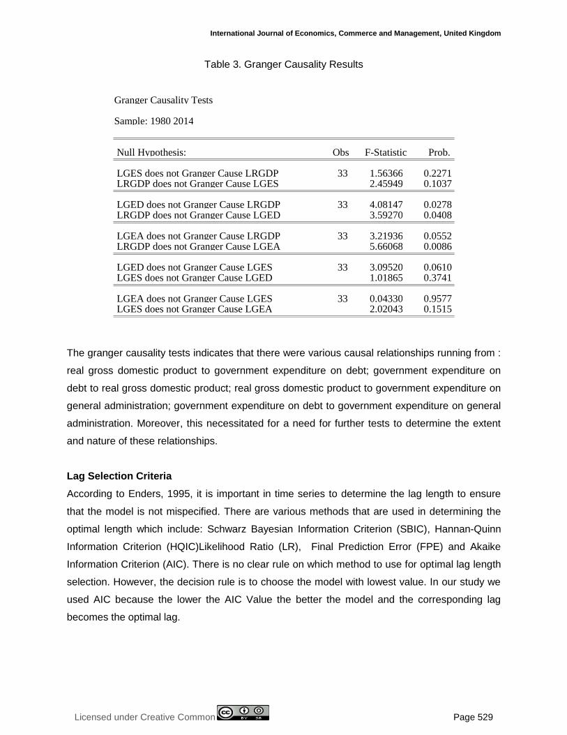
Table 3. Granger Causality Results
The granger causality tests indicates that there were various causal relationships running from :
real gross domestic product to government expenditure on debt; government expenditure on
debt to real gross domestic product; real gross domestic product to government expenditure on
general administration; government expenditure on debt to government expenditure on general
administration. Moreover, this necessitated for a need for further tests to determine the extent
and nature of these relationships.
Lag Selection Criteria
According to Enders, 1995, it is important in time series to determine the lag length to ensure
that the model is not mispecified. There are various methods that are used in determining the
optimal length which include: Schwarz Bayesian Information Criterion (SBIC), Hannan-Quinn
Information Criterion (HQIC)Likelihood Ratio (LR), Final Prediction Error (FPE) and Akaike
Information Criterion (AIC). There is no clear rule on which method to use for optimal lag length
selection. However, the decision rule is to choose the model with lowest value. In our study we
used AIC because the lower the AIC Value the better the model and the corresponding lag
becomes the optimal lag.
Granger Causality Tests Sample: 1980 2014
Null Hypothesis: Obs F-Statistic Prob.
LGES does not Granger Cause LRGDP 33 1.56366 0.2271 LRGDP does not Granger Cause LGES 2.45949 0.1037
LGED does not Granger Cause LRGDP 33 4.08147 0.0278 LRGDP does not Granger Cause LGED 3.59270 0.0408
LGEA does not Granger Cause LRGDP 33 3.21936 0.0552 LRGDP does not Granger Cause LGEA 5.66068 0.0086
LGED does not Granger Cause LGES 33 3.09520 0.0610 LGES does not Granger Cause LGED 1.01865 0.3741
LGEA does not Granger Cause LGES 33 0.04330 0.9577 LGES does not Granger Cause LGEA 2.02043 0.1515
© Mulinge
Licensed under Creative Common Page 530
Autoregressive Distributed Lags Model Test
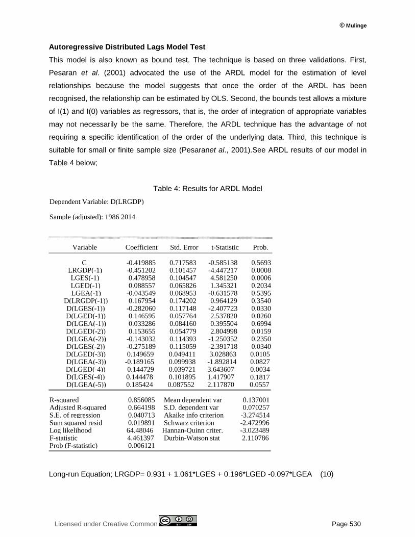
This model is also known as bound test. The technique is based on three validations. First,
Pesaran et al. (2001) advocated the use of the ARDL model for the estimation of level
relationships because the model suggests that once the order of the ARDL has been
recognised, the relationship can be estimated by OLS. Second, the bounds test allows a mixture
of I(1) and I(0) variables as regressors, that is, the order of integration of appropriate variables
may not necessarily be the same. Therefore, the ARDL technique has the advantage of not
requiring a specific identification of the order of the underlying data. Third, this technique is
suitable for small or finite sample size (Pesaranet al., 2001).See ARDL results of our model in
Table 4 below;
Table 4: Results for ARDL Model
Long-run Equation; LRGDP= 0.931 + 1.061*LGES + 0.196*LGED -0.097*LGEA (10)
Dependent Variable: D(LRGDP) Sample (adjusted): 1986 2014
Variable Coefficient Std. Error t-Statistic Prob.
C -0.419885 0.717583 -0.585138 0.5693 LRGDP(-1) -0.451202 0.101457 -4.447217 0.0008 LGES(-1) 0.478958 0.104547 4.581250 0.0006 LGED(-1) 0.088557 0.065826 1.345321 0.2034 LGEA(-1) -0.043549 0.068953 -0.631578 0.5395
D(LRGDP(-1)) 0.167954 0.174202 0.964129 0.3540 D(LGES(-1)) -0.282060 0.117148 -2.407723 0.0330 D(LGED(-1)) 0.146595 0.057764 2.537820 0.0260 D(LGEA(-1)) 0.033286 0.084160 0.395504 0.6994 D(LGED(-2)) 0.153655 0.054779 2.804998 0.0159 D(LGEA(-2)) -0.143032 0.114393 -1.250352 0.2350 D(LGES(-2)) -0.275189 0.115059 -2.391718 0.0340 D(LGED(-3)) 0.149659 0.049411 3.028863 0.0105 D(LGEA(-3)) -0.189165 0.099938 -1.892814 0.0827 D(LGED(-4)) 0.144729 0.039721 3.643607 0.0034 D(LGES(-4)) 0.144478 0.101895 1.417907 0.1817 D(LGEA(-5)) 0.185424 0.087552 2.117870 0.0557
R-squared 0.856085 Mean dependent var 0.137001 Adjusted R-squared 0.664198 S.D. dependent var 0.070257 S.E. of regression 0.040713 Akaike info criterion -3.274514 Sum squared resid 0.019891 Schwarz criterion -2.472996 Log likelihood 64.48046 Hannan-Quinn criter. -3.023489 F-statistic 4.461397 Durbin-Watson stat 2.110786 Prob (F-statistic) 0.006121
International Journal of Economics, Commerce and Management, United Kingdom
Licensed under Creative Common Page 531
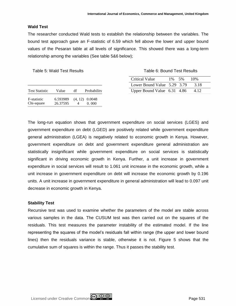
Wald Test
The researcher conducted Wald tests to establish the relationship between the variables. The
bound test approach gave an F-statistic of 6.59 which fell above the lower and upper bound
values of the Pesaran table at all levels of significance. This showed there was a long-term
relationship among the variables (See table 5&6 below);
Table 5: Wald Test Results Table 6: Bound Test Results
The long-run equation shows that government expenditure on social services (LGES) and
government expenditure on debt (LGED) are positively related while government expenditure
general administration (LGEA) is negatively related to economic growth in Kenya. However,
government expenditure on debt and government expenditure general administration are
statistically insignificant while government expenditure on social services is statistically
significant in driving economic growth in Kenya. Further, a unit increase in government
expenditure in social services will result to 1.061 unit increase in the economic growth, while a
unit increase in government expenditure on debt will increase the economic growth by 0.196
units. A unit increase in government expenditure in general administration will lead to 0.097 unit
decrease in economic growth in Kenya.
Stability Test
Recursive test was used to examine whether the parameters of the model are stable across
various samples in the data. The CUSUM test was then carried out on the squares of the
residuals. This test measures the parameter instability of the estimated model. If the line
representing the squares of the model‘s residuals fall within range (the upper and lower bound
lines) then the residuals variance is stable, otherwise it is not. Figure 5 shows that the
cumulative sum of squares is within the range. Thus it passes the stability test.
Critical Value 1% 5% 10%
Lower Bound Value 5.29 3.79 3.18
Upper Bound Value 6.31 4.86 4.12
Test Statistic Value df Probability
F-statistic 6.593989 (4, 12) 0.0048 Chi-square 26.37595 4 0. 000

© Mulinge
Licensed under Creative Common Page 532
Figure 5: CUSUM Test
Normality Tests
The Jarque-Bera statistic was used to test for normality. The statistic gave a probability of more
than 0.05 percent for all the regression equations. Therefore, the null hypothesis, that data is
normally distributed, was accepted.
Figure 6: Normality Test
Heteroscedasticity Test
Heteroscedasticity tests are done on the residuals using Breusch-Pagan-Godfrey specification
to determine homoscedasticity. The Breusch-Pagan-Godfrey regresses squared residuals on
the original regressors by default.
The model R-squared is more than 5% and hence we conclude that the residuals are
homoscedastic. This is a good result for the model.
-12
-8
-4
0
4
8
12
03 04 05 06 07 08 09 10 11 12 13 14
CUSUM 5% Significance
Series: Residuals
Sample: 1986 2014
Observations 29
Mean 1.75e-15
Median -0.002170
Skewness 0.861915
Jarque-Bera 3.921339
Probability 0.140764

International Journal of Economics, Commerce and Management, United Kingdom
Licensed under Creative Common Page 533
Table 7: Heteroscedasticity
Serial Correlation Test
The Breusch –Godfrey serial correlation LM test was done on the system. The R – squared was
found to be more than 5% and therefore there was no serial correlation as shown in the table
below;
Table 8: Serial Correlation results
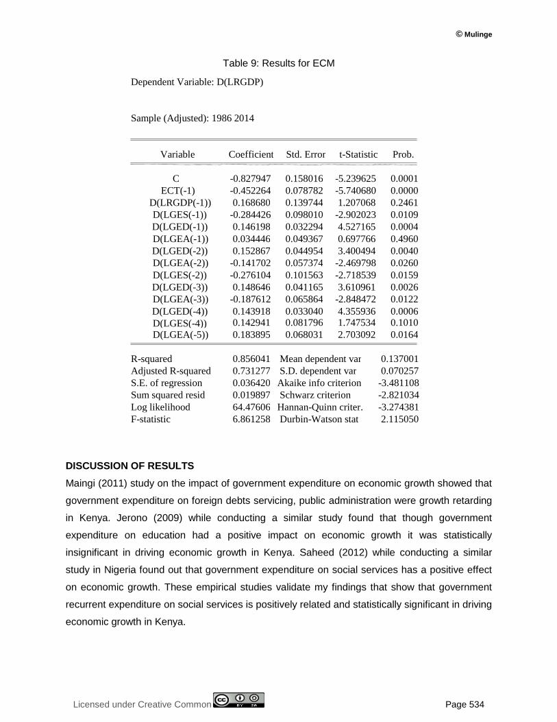
Error Correction Term / Short run relationship
In table 9 above, estimated model passes all diagonistic tests such as normality, serial
correlation and heteroscedasticity (see in appendices 1).The speed of adjustment towards
equillibrium is 45 per cent implying that there will be a sluggish adjustment that will take 2 years
2 months towards equillibrium incase of short-run shocks. The error correction term is highly
significant thus supportive of the specified long-run relationship. The adjusted R-squared is 73
per cent suggesting the error correction model fits the data reasonably well.
Breusch-Godfrey Serial Correlation LM Test:
F-statistic 0.165880 Prob. F(2,14) 0.8488 Obs*R-squared 0.671311 Prob. Chi-Square (2) 0.7149
Heteroskedasticity Test: Breusch-Pagan-Godfrey
F-statistic 0.899266 Prob. F(16,12) 0.5869 Obs*R-squared 15.81231 Prob. Chi-Square(16) 0.4661 Scaled explained SS 3.415621 Prob. Chi-Square(16) 0.9996
© Mulinge
Licensed under Creative Common Page 534
Table 9: Results for ECM
DISCUSSION OF RESULTS
Maingi (2011) study on the impact of government expenditure on economic growth showed that
government expenditure on foreign debts servicing, public administration were growth retarding
in Kenya. Jerono (2009) while conducting a similar study found that though government
expenditure on education had a positive impact on economic growth it was statistically
insignificant in driving economic growth in Kenya. Saheed (2012) while conducting a similar
study in Nigeria found out that government expenditure on social services has a positive effect
on economic growth. These empirical studies validate my findings that show that government
recurrent expenditure on social services is positively related and statistically significant in driving
economic growth in Kenya.
Dependent Variable: D(LRGDP)
Sample (Adjusted): 1986 2014
Variable Coefficient Std. Error t-Statistic Prob.
C -0.827947 0.158016 -5.239625 0.0001
ECT(-1) -0.452264 0.078782 -5.740680 0.0000
D(LRGDP(-1)) 0.168680 0.139744 1.207068 0.2461
D(LGES(-1)) -0.284426 0.098010 -2.902023 0.0109
D(LGED(-1)) 0.146198 0.032294 4.527165 0.0004
D(LGEA(-1)) 0.034446 0.049367 0.697766 0.4960
D(LGED(-2)) 0.152867 0.044954 3.400494 0.0040
D(LGEA(-2)) -0.141702 0.057374 -2.469798 0.0260
D(LGES(-2)) -0.276104 0.101563 -2.718539 0.0159
D(LGED(-3)) 0.148646 0.041165 3.610961 0.0026
D(LGEA(-3)) -0.187612 0.065864 -2.848472 0.0122
D(LGED(-4)) 0.143918 0.033040 4.355936 0.0006
D(LGES(-4)) 0.142941 0.081796 1.747534 0.1010
D(LGEA(-5)) 0.183895 0.068031 2.703092 0.0164
R-squared 0.856041 Mean dependent var 0.137001
Adjusted R-squared 0.731277 S.D. dependent var 0.070257
S.E. of regression 0.036420 Akaike info criterion -3.481108
Sum squared resid 0.019897 Schwarz criterion -2.821034
Log likelihood 64.47606 Hannan-Quinn criter. -3.274381
F-statistic 6.861258 Durbin-Watson stat 2.115050

International Journal of Economics, Commerce and Management, United Kingdom
Licensed under Creative Common Page 535
However, recent studies by Muthui et al (2013) while conducting a similar study in Kenya found
out that government expenditure on health and education is positively related to growth but
statistically insignificant in driving economic growth. My study brings interesting finding to this
debate because it actually conflicts Muthui et al (2013) findings. Would it be government
expenditure on health and education is not properly absorbed when it is development oriented?
Data shows that on average government allocation to the social sectors (education and health)
as a percentage of gross domestic product ranged from 5.3 percent in 1980 to 7.8 percent in
2014.This is a 2.5 percent growth in the expenditures over a span of 34 years, against an
increasing population 16.27 million,1980 and 45 million, 2014. The data also shows that
government expenditure on debt and government expenditure on administration grew over the
same time period by an average of 3.5 per cent and 2 per cent respectively. This is a slow
growth and therefore shows policy makers are cognizant of economic policy implications of the
two variables.
The study finding on this paper urges policy makers to ensure more funds are
concurrently allocated to recurrent components of health and education sectors to spur
economic growth.
Moreover, this study indicates there is a unidirectional relationship between real gross
domestic product and expenditure on debt. Government expenditure on debt is positively
related to growth though statistically insignificant in Kenya. This can be explained by low
productivity of government spending or low absorptive capacity of development expenditure and
therefore full benefits have not yet been realized in the economy. There is also a bidirectional
relationship that runs from government expenditure on debt to government expenditure on
administration. This can be explained by the fact that Kenya is borrowing to finance
development projects hence more resources will be needed for government project
administration. However, the government should not increase its administration workforce
budget through recruiting but they should retain and retrain their current staff.
CONCLUSION
The main objective of this study was to investigate the effect of recurrent public expenditure on
economic growth in Kenya. To achieve the objective of this study, time series data for the period
1980 to 2014 was collected for the various macroeconomic variables. Unit root tests were run to
test the stationarity level of the data which was found to be integrated of order zero, I(0)and
order one, I(1). The data was also tested for cointegration using ARDL model and results
revealed existence of long term relationship between economic growth and its determinants.
According to the Keynesians school of thought, public spending is widely seen as having an
© Mulinge
Licensed under Creative Common Page 536
important role in supporting economic growth in a country. On the other hand, a lower level of
spending implies that fewer revenues are needed to achieve balanced budgets, which means
that lower taxes can be levied, hence contributing to reduction of growth and employment.
Using the collected data, the study showed that government recurrent expenditure on
debt and social services had a positive effect on economic growth in Kenya while government
recurrent expenditure on general public administration had a negative effect. Recurrent public
expenditure on general administration and debt was however statistically insignificant in driving
growth while government recurrent expenditure on social services was statistically highly
significant.
In this study we were investigating the effect of recurrent public expenditure on
economic growth on Kenyan economy using bounds test approach and causality analysis for
annual time series data from 1980-2014.Cointegration test results support long-run relationship
between the macroeconomic variables while granger causality results show that short-run
relationships are evident. The empirical results are in line with the studies of Onotaniyohwo et al
(2012) and Modebe (2012) et al that recurrent government expenditure components had
positive and negative impacts on economic growth in Nigeria.
RECOMMENDATIONS
Several policy implications can be derived from understanding directions and magnitude of
causality between government expenditure on debt and economic growth. The trends in
government borrowing have tremendously increased in the recent years; however growth has
maintained an average of 5.41 per cent for the last 10 years. The government should borrow
and invest into public projects that are growth promoting in any part of the country without
political coercions.
Possibly there could be lack of accountability of public expenditures by government
officials especially in handling public borrowed funds and this could explain why recurrent
expenditure components have always been seen to retard growth. Those who hold powerful
positions should account for every shilling that is invested in any project. The expenditures must
be sound and within limits. The government should also strengthen Ethics and Anti-corruption
commissions to ensure that they have prosecution powers to prosecute any corrupt mal
practices. This will help Kenya to realize all positive effects that come with public debt as a
result of prudence in the management of borrowed funds.
The government through the Ministry of Finance should come up with frameworks to
give a direction to the National and County Treasuries on recurrent and development
expenditure limits. The commission should also have a framework that gives the counties a

International Journal of Economics, Commerce and Management, United Kingdom
Licensed under Creative Common Page 537
direction on specific projects to undertake in a financial year. In this framework, project
undertakings can be tilted or increased towards social sectors since they promote economic
growth both in the short-run and long-run.
The study also recommends that allocations into general administration of the
government should be reduced to support projects that are growth promoting. According to the
Institute of Economic Affairs (IEA, 2014) Kenyan public officials are among the best paid in
Africa. Government recurrent expenditure on administration is negatively related to growth thus
the government should come up with strategies that increase administrative output to promote
the national gross domestic product.
SUGGESTIONS FOR FURTHER RESEARCH
The study only considered the recurrent government expenditure components in various
selected sectors (education, health, administration and public debt).However; other sectors,
which include; agriculture, Security, environment and natural resources play a critical role in
economic growth of the nation and therefore should also be examined to evaluate the current
contributions and impacts they offer to growth.
Further, the researcher also recommends a study on the budgeting and actual
expenditure allocations on operations and maintenance item in the budget and its impact on
growth. This expenditure item is set to increase tremendously in the next decade due to many
infrastructural projects being undertaken by the government in the country. This will ensure that
they are structured to promote growth in the economy.
REFERENCES
Agénor, P. R. (2008). Health and infrastructure in a model of endogenous growth. Journal of Macroeconomics, 30(4), 1407-1422.
Alexander, C. (2001). Market models: A guide to financial data analysis. John Wiley & Sons.
Barro, R. J., &Sala-i-Martin, X. (1990).Economic Growth and Convergence across the United State.NBER Working paper, (3419).
Chude, A., &Chude, E. (2013).Effect of Government Expenditure on Economic Growth in Nigeria. Lagos: Unpublished.
Degefe, B. (1992). Growth and foreign debt: The Ethiopian experience: 1964-86 (No. RP_13).
Devarajan, S., Swaroop, V., &Zou, H. F. (1996). The composition of public expenditure and economic growth. Journal of monetary economics, 37(2), 313-344.
Dimitrova, D. (2005). The relationship between exchange rates and stock prices: Studied in a multivariate model. Issues in Political Economy, 14(1), 3-9.
Easterly, W. (2005). National policies and economic growth: a reappraisal. Handbook of economic growth, 1, 1015-1059.
© Mulinge
Licensed under Creative Common Page 538
Elahi, M., &Dehdashti, M. (2011).Classification of researches and evolving a consolidating typology of management studies. In Proceedings of the 2011 Annual Conference on Innovations in Business & Management.
Elbadawi, A., &Ndulu, B. (1996).Long run development and sustainable growth in Sub- Saharan Africa. New Directions in Development Economics: Growth, Environmental Concerns and Governments in the 1990s.
GoK (1997).‗Public Expenditure Review‘. Nairobi: Public Expenditure Review Secretariat, Ministry of Finance. Mimeo.
Granger, C. W., & Newbold, P. (1974).Spurious regressions in econometrics. Journal of econometrics, 2(2), 111-120.
IEA (2014): Public sector wages. Nairobi, Kenya. Institute of economic affairs.
Jerono, A. (2009).Impact of public expenditure on economic growth in Kenya. Unpublished. Kenyatta University. Nairobi, Kenya.
Johansen, S., &Juselius, K. (1990).Maximum likelihood estimation and inference on cointegration with applications to the demand for money. Oxford Bulletin of Economics and statistics, 52(2), 169-210.
KNBS (2013). Economic Survey 2013. Nairobi, Kenya: Kenya National Bureau of Statistics.
KNBS (2014).Economic Survey 2014.Nairobi, Kenya: Kenya National Bureau of Statistics.
KNBS (2015).Economic Survey 2015. Nairobi, Kenya: Kenya National Bureau of Statistics.
Kuştepeli, A. P. Y. (2005). The relationship between government size and economic growth: evidence from a panel data analysis. Dokuz Eylül University.
Loto, M. A. (2011). Impact of government sectoral expenditure on economic growth. Journal of Economics and international Finance, 3(11), 646-652.
M'Amanja, D., & Morrissey, O. (2005).Fiscal policy and economic growth in Kenya. Centre for Research in Economic Development and International Trade, University of Nottingham.
Maingi, N. J. (2011). The impact of government expenditure on economic growth in Kenya: 1963-2008 (Doctoral dissertation).
Musgrave, R. A. (1959). Theory of public finance; a study in public economy.
Maysami, R. C., Howe, L. C., & Hamzah, M. A. (2004). Relationship between macroeconomic variables and stock market indices: Cointegration evidence from stock exchange of Singapore‘s All-S sector indices. Jurnal Pengurusan, 24(1), 47-77.
Mbanga, G., & Sikod, F. (2001, May). The impact of debt and debt-service payments on investment in Cameroon. In Final report presented at the AERC Biannual Research Workshop, May (pp. 26-31).
Mbire, B., and M. Atingi (1997). ‗Growth and Foreign Debt: The Ugandan Experience.‘ AERC Research Paper No. 66. Nairobi.
Modebe, N. J., Okafor, R. G., Onwumere, J. U. J., &Ibe, I. G. (2012). Impact of recurrent and capital expenditure on Nigeria‘ economic growth. European Journal of Business and Management, 4(19), 66-75.
Mugenda, A. G. (2008). Social science research: Theory and principles. Nairobi: Applied.
Muthui, J. N., Kosimbei, G., Maingi, J., &Thuku, G. K. (2013). The Impact of Public Expenditure Components on Economic Growth in Kenya 1964-2011. International Journal of Business and Social Science, 4(4)
Ndoma-Egba, V. (2012).Legislative oversight and public accountability. University of Nigeria, Nsuka, Enugu State, Nigeria.
Ndonga, I. K. (2014). Effects of government spending on economic growth in Kenya (Doctoral dissertation, University of Nairobi).

International Journal of Economics, Commerce and Management, United Kingdom
Licensed under Creative Common Page 539
Ngechu, M. (2004). Understanding the research process and methods: An introduction to Research Methods.
Nurudeen, A., &Usman, A. (2010). Government expenditure and economic growth in Nigeria, 1970-2008: A disaggregated analysis. Business and Economics Journal, 2010, 1-11.
Peacock, A. T., & Wiseman, J. (1961). Front matter, The Growth of Public Expenditure in the United Kingdom. In The growth of public expenditure in the United Kingdom (pp. 32-0). Princeton University Press.
Pesaran, M. H., Shin, Y., & Smith, R. J. (2001).Bounds testing approaches to the analysis of level relationships. Journal of applied econometrics, 16(3), 289-326.
Republic of Kenya. (2003). Economic Recovery Strategy Paper for Wealth and Employment Creation. Nairobi, Kenya: Government printers.
Republic of Kenya. (2002). National Development Plan. Nairobi, Kenya: Government Printers.
Republic of Kenya. (2001). Poverty Reduction Strategy Paper (PRSP) for the Period 2001-2004. Nairobi, Kenya: Government Printers.
Republic of Kenya. (2008). Kenya Vision 2030. Nairobi, Kenya: Government Printers.
Saheed, Z. S., & Ayodeji, S. (2012). Impact of Capital Flight on Exchange Rate and Economic Growth in Nigeria. International Journal of Humanities and Social Sciences, 2, 13.
Simiyu, C. N. (2015). Essays explaining Impact of public expenditure on economic growth in Kenya.
Stiglitz, J. E., Vieira, L. F., Hatwich, F., Arévalo, V., Andino, M., Grijalva, J., & Piñeiro, A. M. (2000).Economics of the public sector (No. 336.73 S855 2000). ISNAR, La Haya (PaísesBajos). IICA, San José (Costa Rica).
Stiglitz, J. E. (1989). The economic role of the state.
Wagner, R. E., & Warren, E. W. (1977). Wagner‘s law, Fiscal institutions, and the growth of the government. National Tax Journal, 30(1), 59–68. Retrieved from http://www.jstor.org
Were, M. (2001).The impact of external debt on economic growth in Kenya. UNU-WIDER Research Paper, DP, 116.
Zimmerman, C. C. (1932). Ernst Engel's law of expenditures for food. The Quarterly Journal of Economics, 78-101.
APPENDIX: DIAGONISTICS FOR ECM
Normality Test
0
2
4
6
8
10
-0.04 -0.02 0.00 0.02 0.04 0.06
Series: Residuals
Sample 1986 2014
Observations 29
Mean 1.31e-16
Median -0.002242
Maximum 0.060773
Minimum -0.039409
Std. Dev. 0.026657
Skewness 0.878484
Kurtosis 3.528163
Jarque-Bera 4.067117
Probability 0.130869
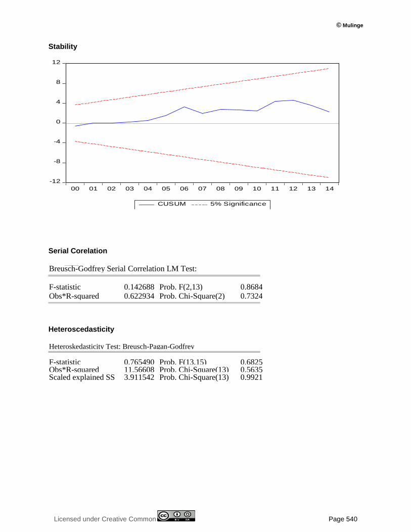
© Mulinge
Licensed under Creative Common Page 540
Stability
Serial Corelation
Heteroscedasticity
-12
-8
-4
0
4
8
12
00 01 02 03 04 05 06 07 08 09 10 11 12 13 14
CUSUM 5% Significance
Heteroskedasticity Test: Breusch-Pagan-Godfrey
F-statistic 0.765490 Prob. F(13,15) 0.6825 Obs*R-squared 11.56608 Prob. Chi-Square(13) 0.5635 Scaled explained SS 3.911542 Prob. Chi-Square(13) 0.9921
Breusch-Godfrey Serial Correlation LM Test:
F-statistic 0.142688 Prob. F(2,13) 0.8684 Obs*R-squared 0.622934 Prob. Chi-Square(2) 0.7324