Effects of minimum quantity lubrication (MQL) on tool …/67531/metadc149638/m2/1/high...Maru,...

APPROVED: Nourredine Boubekri, Major Professor Seifollah Nasrazadani, Committee Member Leticia Anaya, Committee Member Enrique Barbieri, Chair of the Department of

Engineering Technology Costas Tsatsoulis, Dean of the College of

Engineering Mark Wardell, Dean of the Toulouse Graduate

School

EFFECTS OF MINIMUM QUANTITY LUBRICATION (MQL) ON TOOL LIFE IN

DRILLING AISI 1018 STEEL

Tejas Maru, B.E.

Thesis Prepared for the Degree of

MASTER OF SCIENCE

UNIVERSITY OF NORTH TEXAS

August 2012

Maru, Tejas. Effects of minimum quantity lubrication (MQL) on tool life in

drilling AISI 1018 steel. Master of Science (Engineering Systems-Mechanical Systems),

August 2012, 73 pp., 17 tables, 36 figures, references, 27 titles.

It has been reported that minimum quantity lubrication (MQL) provides better

tool life compared to flood cooling under some drilling conditions. In this study, I

evaluate the performance of uncoated HSS twist drill when machining AISI 1018 steel

using a newly developed lubricant designed for MQL (EQO-Kut 718 by QualiChem

Inc.). A randomized factorial design was used in the experiment. The results show that a

tool life of 1110 holes with a corresponding flank wear of 0.058 mm was realized.

ii

Copyright 2012

by

Tejas Maru

iii

ACKNOWLEDGEMENTS

I am very thankful to my major professor Dr. Nourredine Boubekri for his

encouragement, suggestions, guidance and support for this research work. His support

and guidance assisted me in successfully completing this research work.

I thank Dr. Phillip Foster for his assistance with the CNC machine and its

programming operations. I am grateful for his cooperation and willingness to answer any

questions without hesitation.

I am thankful to other committee members: Dr. Anaya Leticia for helping me to

understand the statistical part in the research work and guiding me in thesis writing and

Dr. Seifollah Nasrazadani for his valuable timing to guiding me and reviewing my thesis.

I am also thankful to my family for being with me and for supporting me through

out my life.

iv

TABLE OF CONTENTS

Page

ACKNOWLEDGEMENTS ............................................................................................... iii LIST OF TABLES ............................................................................................................. vi LIST OF FIGURES ......................................................................................................... viii CHAPTER I INTRODUCTION ........................................................................................ 1 CHAPTER II LITERATURE REVIEW ........................................................................... 5

Summary ............................................................................................................... 22 CHAPTER III EXPERIMENTAL METHOD AND PROCEDURE .............................. 24

Objectives ............................................................................................................. 24

Design of Experiments .......................................................................................... 24

Cutting Tool .......................................................................................................... 26

Coolant .................................................................................................................. 26

Sample Preparation ............................................................................................... 28

Drilling Equipment ............................................................................................... 34

Work Piece Material ............................................................................................. 35

Drilling Procedure ................................................................................................. 36

Data Collection Method ........................................................................................ 38

Inner Diameter Measurement Procedure .............................................................. 38

Data Analysis ........................................................................................................ 39

Tool Failure Analysis ............................................................................................ 40

Main Assumption of Study ................................................................................... 40 CHAPTER V ANALYSIS ............................................................................................... 42

Hypothesis............................................................................................................. 42

Correlation Analysis ............................................................................................. 47

Tool Life Analysis ................................................................................................ 58

v

Tool Failure Analysis ............................................................................................ 61

Summary ............................................................................................................... 65 CHAPTER VI CONCLUSION ....................................................................................... 68

Recommendations for Future Research ................................................................ 69 REFERENCES ................................................................................................................. 70

vi

LIST OF TABLES

Page

Table 1 The corner wear and flank wear for P35 and P25 tool under different cutting

environment [8]. .......................................................................................................... 6

Table 2 Effect of different cutting speed on wear [8]. ........................................................ 7

Table 3 Effect of cutting environment on flank wear and surface roughness [9]. .............. 8

Table 4 Effect of different cutting speeds and feed rates on tool life under different

lubrication environment [10]. ..................................................................................... 9

Table 5 Cutting parameters used in the experiment [12]. ................................................. 11

Table 6 Effects of cutting environment on tool life of flat-faced PVD tools and grooved

PVD tools [16]. ......................................................................................................... 15

Table 7 Effects of cutting speeds and feed rates on tool life under dry and MQL cutting

environment [21]. ...................................................................................................... 17

Table 8 Effects of cutting speeds on cutting force and surface roughness in dry and MQL

cutting environment [22]........................................................................................... 18

Table 9 Effect of cutting speeds and feed rates on tool life [25]. ..................................... 21

Table 10 Speed and feed rate combination. ...................................................................... 25

Table 11 Chemical composition of AISI 1018 steel (Source: Lokey Metals, FW). ......... 35

Table 12 Mechanical properties of AISI 1018 steel (Source: Lokey Metals, FW). ......... 35

Table 13 ANOVA analysis table for hole-diameter. ........................................................ 45

Table 14 Coefficient of correlation for the Combination 1. ............................................. 49

vii




viii

LIST OF FIGURES

Page

Figure 1 MQL system. ........................................................................................................ 2

Figure 2 Internally applied MQL. ....................................................................................... 3

Figure 3 Externally applied MQL. ...................................................................................... 4

Figure 4 HSS drill. ............................................................................................................ 26

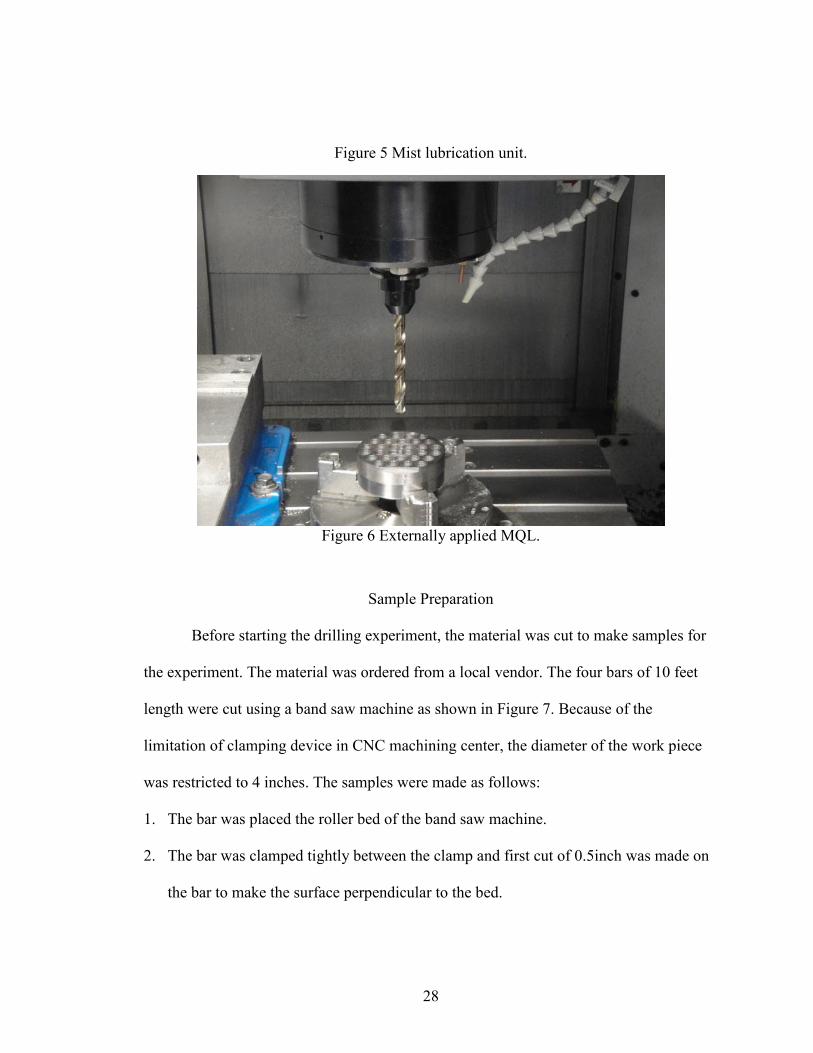
Figure 5 Mist lubrication unit. .......................................................................................... 28

Figure 6 Externally applied MQL. .................................................................................... 28

Figure 7 Band saw cutting (Source: MFET Lab, UNT). .................................................. 30

Figure 8 Blank from bar. ................................................................................................... 30

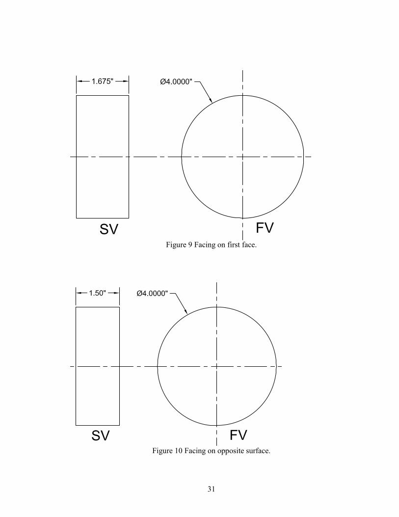
Figure 9 Facing on first face. ............................................................................................ 31

Figure 10 Facing on opposite surface. .............................................................................. 31

Figure 11 Work piece for experiment. .............................................................................. 32

Figure 12 Work piece layouts. .......................................................................................... 33

Figure 13 Drilling equipment (Source: MFET Lab, UNT)............................................... 34

Figure 14 Flank wear measurement. ................................................................................. 40

Figure 15 Normal probability plot. ................................................................................... 43

Figure 16 Predicted vs. residual graph. ............................................................................. 44

Figure 17 Hole-diameter vs. number of holes (80SFM, 0.003IPR).................................. 47

Figure 18 Hole-diameter for first hundred holes (80SFM, 0.003IPR). ............................ 48

Figure 19 Hole-diameter for last hundred holes (80SFM, 0.003IPR). ............................. 48

ix

Figure 20 Hole-diameter vs. number of holes (80SFM, 0.004IPR).................................. 51

Figure 21 Hole-diameter for first hundred holes (80SFM, 0.004IPR). ............................ 51

Figure 22 Hole-diameter for last hundred holes (80SFM, 0.004IPR). ............................. 52

23 Hole-diameter vs. number of holes (120SFM, 0.003IPR). .......................................... 53

Figure 24 Hole-diameter for first hundred holes (120SFM, 0.003IPR). .......................... 54

Figure 25 Hole-diameter for last hundred holes (120SFM, 0.003IPR). ........................... 54

Figure 26 Hole-diameter vs. number of holes (120SFM, 0.004IPR)................................ 56

Figure 27 Hole-diameter for first hundred holes (120SFM, 0.004IPR). .......................... 56

Figure 28 Hole-diameter for last hundred holes (120SFM, 0.004IPR). ........................... 57

Figure 29 Feed-rate vs. tool life. ....................................................................................... 58

Figure 30 Cutting speed vs. tool life. ................................................................................ 59

Figure 31 Tool-life for different mist lubrication. ............................................................ 60

Figure 32 Tool-failure for first combination. .................................................................... 61

Figure 33 Tool-failure for second combination. ............................................................... 62

Figure 34 Tool-failure for third combination-a. ............................................................... 63

Figure 35 Tool-failure for third combination- b. .............................................................. 64

Figure 36 Tool-failure for fourth combination. ................................................................ 64

1

CHAPTER I

INTRODUCTION

Heat is generated during machining in considerable amounts because of the

cutting action and friction created by the tool, the work piece and the chips. It is

important to reduce the heat generated to improve the tool’s life and its dimensional

accuracy, to increase the material removal rate, to reduce the cutting forces and to

improve the surface roughness of the work piece. Coolant or cutting fluid is used to take

away the heat and to lubricate the machined surface. Cutting fluid should promote the

tool life, improve the surface integrity of the work piece, flush the chips from the cutting

zone and protect the surface from corrosion [1]. Traditionally, the machining of parts

uses flood cooling in which the jet of coolant is directed toward the cutting zone. Here,

the coolant is deployed in large quantities. There are several disadvantages to using this

method. The first one has to do with the cost of machining and its disposal.

Approximately fifteen percent of total cost in machining is incurred by the coolant and its

disposal [2]. The second one deals with a safety issue for the operators. One problem that

exists for operators is that when they stay in contact with the coolant for a long time, it

may cause skin problems. The third one is the effect on the environment. After

machining, the chips produced are mixed with the cutting fluid and they cannot be

disposed of directly as regular trash. At the same time, coolant should be filtered before

being reused and after several more uses, the coolant also needs to be disposed.

2

The chips and the used coolant are disposed as hazardous waste-a practice that is

costly to any industry. Hence, using the coolant in large quantities is a costly proposition

that is not user friendly nor environmental friendly. The alternative solution is to machine

with a minimum quantity of lubrication (MQL). MQL is also known as near dry

machining or spatter lubrication [1,4].

MQL technique uses a small quantity of oil or lubricant. It is mixed with

compressed air to generate a mist or an aerosol. The mist particles provide lubrication

and the compressed air helps to reduce the temperature during machining. The range of

oil flow rate in MQL usually varies from 1oz to 8oz in 8 hour [3, 4]. This quantity is very

small compared to flood cooling. The air pressure varies from 0.2MPa to 6-bar. The

selection of the parameters basically depends on the type of tool material, the work piece

material and the processes.

Figure 1 MQL system.

3

MQL can be applied internally or externally as shown in Figure 2 and 3

respectively. In the internal way of applying MQL, mist is passed through the spindle,

tool holder and tool. There are two basic approaches for applying MQL internally. In one

method, oil and compressed air are mixed in an external unit and passed through the

spindle and tool holder. In the other approach, the oil and the compressed air are mixed

inside the spindle and passed through the tool holder. In the external way of applying

MQL, the oil is mixed with the compressed air in one external unit and is deployed

through an external jet. This system is simple, less expensive and effective for drilling

shallow holes and low speed processes like gear cutting and broaching [3].

Figure 2 Internally applied MQL.

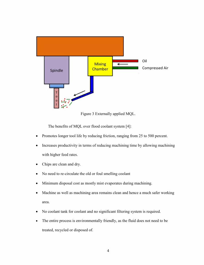
4

Figure 3 Externally applied MQL.

The benefits of MQL over flood coolant system [4]:

• Promotes longer tool life by reducing friction, ranging from 25 to 500 percent.

• Increases productivity in terms of reducing machining time by allowing machining

with higher feed rates.

• Chips are clean and dry.

• No need to re-circulate the old or foul smelling coolant

• Minimum disposal cost as mostly mist evaporates during machining.

• Machine as well as machining area remains clean and hence a much safer working

area.

• No coolant tank for coolant and no significant filtering system is required.

• The entire process is environmentally friendly, as the fluid does not need to be

treated, recycled or disposed of.

5

CHAPTER II

LITERATURE REVIEW

AISI 1018 steel has many applications. One of them is the manufacturing of

bolts, gears, pinions, shafts, ratchet, machine parts, and axles. Most these parts are

produced through machining processes such as turning, drilling, milling, shaping and

grinding. It has been noticed that 70-80% of the manufactured parts need machining

before the actual applications [5]. In machining, cooling and lubricating methods play an

important role in minimizing the heat-affected zone. Traditionally, a flood cooling system

is used to reduce the temperature of the cutting tool during the machining process. Due to

high cutting forces and tool-work piece interface temperature, both work materials and

tool materials may diffuse into each other. Either the chips take away the tool’s material

or the chip particles diffuse onto the tool tip. As a consequence, many failures such as

flank wear, thermal cracks and chipping occur on the cutting tool. In a flood cooling

system, a large amount of coolant is required which increases the cost of machining. It is

also hazardous in industrial applications. Nowadays, industries opt for Minimum

Quantity Lubrication (MQL) system. In a MQL system, mist is generated and the flow of

mist is regulated for optimum results. This system has proved to be more efficient and

more economical compared to the flood coolant system [6,7].

The application of MQL is found more effective than flood cooling lubrication

systems in grooving operations. Air supply plays a vital role in mist transportation to the

tool and work piece interface area.

6

Obikawa et al. [8] conducted an experiment in 2005 on 0.45% carbon steel with

TiC/TiCN/TiN triple layer coated carbide tool. The comparison was done between a P35

coated cemented carbide tool and a P25 uncoated cemented carbide tool. In the

experiment, a P35 tool was used for a 3000 am cutting length and a P25 tool was used for

a 1000 m cutting length. Two cutting speeds were used: 4 m/sec and 5 m/sec. The feed

rate was 0.12 mm/rev. MQL was applied at the rate of 7 ml/h and the flow rate for the

controlled-oil-mist directed grooving tool (COD tool) was set to 2.4 ml/h. The corner

edge-wear and flank wear was measured in dry, wet and MQL cooling conditions. Three

different air pressures were used: 0.3MPa, 0.5MPa and 0.7MPa. When the cutting speed

was 4 m/sec, the feed rate was set to 0.12 mm/rev and the air pressure was set to 0.7MPa.

The corner wear and flank wear for the P35 and P25 tools under dry; wet and MQL

cutting are listed on Table 1.

Table 1 The corner wear and flank wear for P35 and P25 tool under different cutting environment [8].

P35 tool Corner

wear Flank wear P25 tool

Corner

wear Flank wear

MQL 0.05mm 0.03mm MQL 0.24mm 0.19mm

Wet 0.12mm 0.06mm Dry 0.22mm 0.16mm

Dry 0.15mm 0.08mm

From these results, it can be said that the wear is minimum in MQL compared to

wet cooling and dry cutting conditions for P35 tool. There is not much difference in wear

for the uncoated carbide tool. To see the effect of cutting speed, the experiment was

7

further run with a P35 coated carbide tool and the cutting speed being set at 4 m/sec and

then 5 m/sec. The data obtained is listed on Table 2.

Table 2 Effect of different cutting speed on wear [8].

Cutting speed Corner wear Flank wear Cutting length

4 m/sec- MQL 0.06 mm 0.04 mm 3300 m

5 m/sec- Dry 0.17 mm 0.08 mm 2700 m

4 m/sec- MQL 0.14 mm 0.06mm 2600 m

5 m/sec- Dry 0.16 mm 0.10 mm 2100 m

From Table 2, it can be said that at the higher cutting speed of 5 m/sec, the corner

wear in dry cutting increased suddenly due to the loss of coating layers. MQL reduced the

wear to a large extent even at high cutting speed of 5 m/sec. The results also showed that

by increasing the air pressure in MQL from 0.3 MPa to 0.7 MPa, flank wear and corner

wear reduced drastically with a constant supply of MQL by 7ml/h.

The application of MQL in turning operation reduces tool wear, surface roughness

and cutting temperature at the tool-chip-work piece surface contact as reported by Dhar et

al. [9], who conducted an experiment on the turning of AISI 4340 steel. Here, Machining

was done with carbide inserts at a cutting speed of 110 m/min, a feed rate of 0.16 mm/rev

and a depth of cut of 1.5 mm. The turning operation was done under a dry, wet (flood

cooling) and MQL environment. In MQL, the air pressure was set to 7-bar and the flow

rate at 60 ml/h. The machining was done for about 45 min. During the experiment, the

average principal flank wear, average auxiliary flank wear and surface roughness were

8

measured for different cutting lengths. Table 3 lists the results for a 45 min cutting

length:

Table 3 Effect of cutting environment on flank wear and surface roughness [9].

Environment Avg. principal flank

wear (µm)

Avg. auxiliary flank

wear (µm)

Surface roughness Ra

(µm)

Dry 475 375 52

Wet 500 450 60

MQL 350 325 45

From Table 3, it can be said that the wear rate and the surface roughness value

were lesser in MQL compared to dry and wet cooling conditions. The growth rate of the

flank wears decreased in MQL because of the reduction in temperature at the tool-chip

interface area near the flank surface of the tool. Reduction in temperature helped to

reduce abrasion wear by retaining tool hardness and also helped to reduce abrasion and

diffusion types of wear-which are highly sensitive to temperature. The surface finish of

the work piece and the dimensional accuracy depend on the auxiliary flank wear [9].

In 2005, Attanasio et al. [10] applied MQL technique on rake surfaces and flank

surfaces of the tool to see the effect of wear on the tool. The turning operation was done

on 100Cr6-normalized steel with feed rates of 0.2 mm/rev and 0.26 mm/rev, a cutting

speed of 300 m/min, a depth of cut of 1mm, and cutting lengths of 50 mm and 200 mm.

Three different lubrication systems were used: dry, MQL on flank surface and MQL on

rake surface. In MQL, ester oil with EP additive (COUPEX EP46) was used with an air

9

pressure of 2.5bar and an oil flow rate of 20 mg/h. Tool life was recorded in minutes for

different combinations of feed rates, cutting lengths and lubrication systems.

Table 4 Effect of different cutting speeds and feed rates on tool life under different lubrication environment [10].

Lubrication

Environment

Tool life when

feed rate: 0.2

mm/rev and

cutting length:

50 mm

Tool life when

feed rate: 0.26

mm/rev and

cutting length:

50 mm

Tool life when

feed rate: 0.20

mm/rev and

cutting length:

200 mm

Tool life when

feed rate: 0.26

mm/rev and

cutting length:

200 mm

Dry cutting 10.04 min 8.17 min 10.10 min 7.86 min

MQL on Rake 9.75 min 8.58 min 9.28 min 9.36 min

MQL on Flank 10.36 min 9.16 min 11.44 min 9.68 min

From Table 4 it was observed that the maximum tool life was obtained when

MQL was applied on the flank surface of the tool with a feed rate of 0.2 mm/rev. As feed

rate increased to 0.26 mm/rev, the tool life was reduced to 9.68 min. The tool tips were

observed under scanning electron microscope (SEM). On the rake surface crater wear, the

inner notching and outer notching were observed. Under energy dispersive x-ray (EDS)

analysis, elements like sulphur and calcium were observed on the tip used in flank MQL.

Those elements were not present on the tip used in rake MQL. This indicates that MQL

was not able to reach at the cutting area when it was applied on the rake surface. The

team had concluded that MQL gives some advantages during the turning operation but it

has some limitation due to the difficulty of the lubricants reaching the cutting surface.

10

Dhar et al. [11] showed that MQL helps to reduce the cutting temperature and

dimensional inaccuracy when turning of AISI 1040 steel was cut by an uncoated carbide

insert. The results obtained in MQL were compared with dry cutting and wet cooling

conditions. Different sets of cutting speeds and feed rates were used to compare the

effectiveness of dry, wet and MQL cooling conditions. The air pressure of 7-bar and a

flow rate of 60 ml/h were used in MQL. Cutting speeds were: 64, 80, 110 and 130 m/min

and feed rates were: 0.1, 0.13, 0.16 and 0.2 mm/rev. The effectiveness of the cooling

media was observed by measuring the tool-chip interface temperature, the chips’ shapes

and color, the chip reduction co-efficient and the dimensional deviation at different

cutting speeds and feed rates. The tool-chip interface temperature was observed to be the

lowest when machining was done with a feed rate of 0.1 mm/rev and a cutting speed of

130 m/min under MQL. When the feed rate was set to 0.2 mm/rev, the temperatures were

recorded as 790°C, 775°C and 760°C for dry, wet and MQL conditions respectively. The

trend of cutting temperature decreased when the feed rates and cutting speeds were

decreased. To determine the dimensional accuracy, the experiment was run at the cutting

speed of 110 m/min, a feed rate at 0.2 mm/rev and a depth of cut at 1mm. It was observed

that for a cutting length of 425mm, the dimensional deviation was minimum (about

70µm) under MQL and maximum (95µm) under dry cutting condition. The study

concluded that MQL provides benefits mainly due to the reduction in cutting

temperature, which improves the tool-chip interaction and maintains the sharpness of the

cutting edges. MQL reduced tool tip wear and damages and because of this, dimensional

accuracy improved.

11

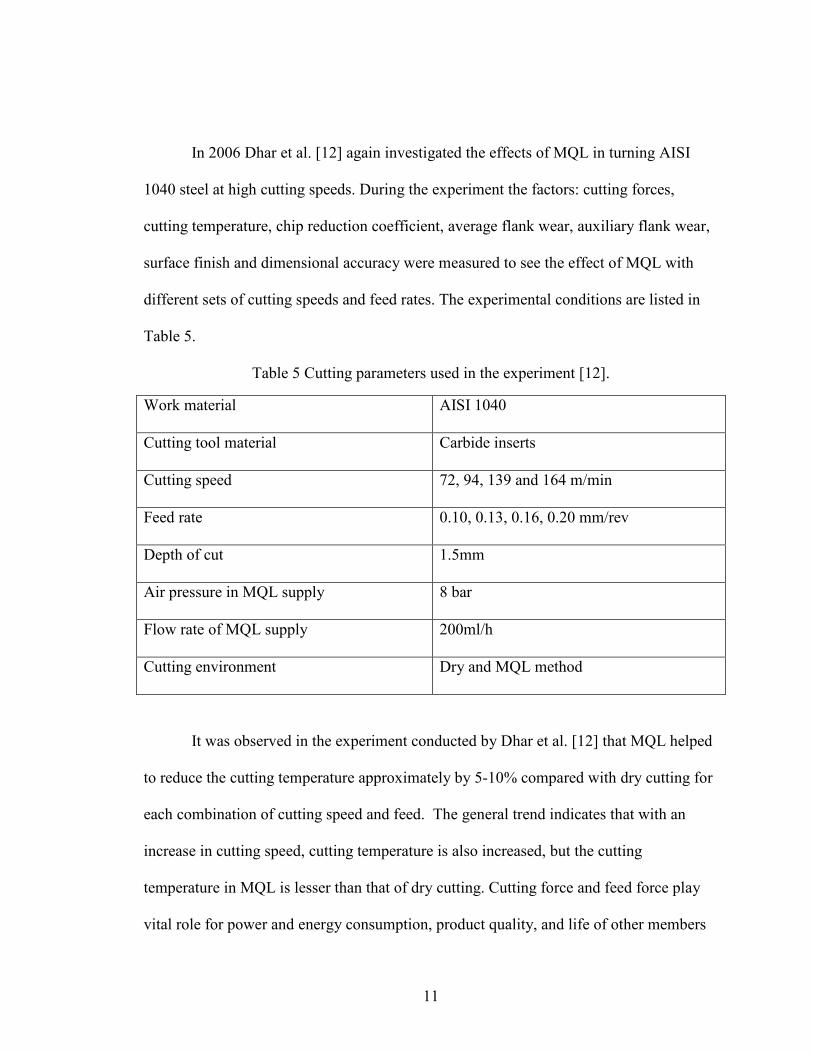
In 2006 Dhar et al. [12] again investigated the effects of MQL in turning AISI

1040 steel at high cutting speeds. During the experiment the factors: cutting forces,

cutting temperature, chip reduction coefficient, average flank wear, auxiliary flank wear,

surface finish and dimensional accuracy were measured to see the effect of MQL with

different sets of cutting speeds and feed rates. The experimental conditions are listed in

Table 5.

Table 5 Cutting parameters used in the experiment [12].

Work material AISI 1040

Cutting tool material Carbide inserts

Cutting speed 72, 94, 139 and 164 m/min

Feed rate 0.10, 0.13, 0.16, 0.20 mm/rev

Depth of cut 1.5mm

Air pressure in MQL supply 8 bar

Flow rate of MQL supply 200ml/h

Cutting environment Dry and MQL method

It was observed in the experiment conducted by Dhar et al. [12] that MQL helped

to reduce the cutting temperature approximately by 5-10% compared with dry cutting for

each combination of cutting speed and feed. The general trend indicates that with an

increase in cutting speed, cutting temperature is also increased, but the cutting

temperature in MQL is lesser than that of dry cutting. Cutting force and feed force play

vital role for power and energy consumption, product quality, and life of other members

12

such as the tool holder, the fixtures and other machine parts. It was observed that as

cutting speed increased, the magnitude of both of these forces reduced. In comparison

between dry cutting and MQL, MQL helped to reduce these forces. During the

machining, the shear strength of the material increases due to compression and straining.

If cutting temperature is high enough shear strength of the material decreases due to

softening effect. Overall cutting forces depend on the type of material, the cutting

temperature, the fixtures and the mountings. MQL helps to reduce the cutting temperature

and hence, results in reduced forces. The tool life affects the productivity and economy of

manufacturing. When tool inserts were observed, the rake surface and the clearance

surface had crater wear and flank wear respectively due to the continuous interaction and

rubbing action between chips and the work surface. The flank wears, surface roughness

and dimensional deviation were found to be lesser with the use of MQL compared to dry

cutting. Overall it was observed that when MQL was used in the turning of AISI 1040

steel, tool life was increased. At the same time, cutting forces, flank wear, surface

roughness and dimensional deviation were decreased.

Dhar et al. [13] conducted another study on AISI 1060 steel in which all the

parameters were kept the same as in the previous study except for the work piece

material, the air pressure and the flow rate of MQL. Here, air pressure was set at 7-bar

and flow rate was set at 60 ml/h. The experiment was run under dry cutting and MQL

cutting environments. It was observed that MQL helped to reduce the average cutting

temperature by 5% to 12% depending upon the process parameters (i.e. feed rate and

cutting speed). The authors also discovered that as the cutting speed increased, the

13

accumulation of chips made it difficult for the proper amount of MQL to reach the

cutting zone. In conventional machining, the tool generally failed by gradual wears due to

abrasion, adhesion, diffusion, chemical erosion and galvanic action that depend on the

type of tool, the tool material and the work piece material. The growth of average flank

wear under MQL was lesser than that of dry cutting condition. But as the machining time

increased, the flank-wear also increased. Dimensional deviation and surface roughness

were also found to be more in dry cutting than under MQL cutting. Overall, MQL gave

better results for cutting forces, tool wear, surface roughness and dimensional deviation.

The location of MQL jet also plays a major role during machining. The position

of the nozzle affects the cutting temperature during machining. To determine the effect of

angle at which the MQL nozzle is set on the machining temperature, Ueda et al. [14]

conducted one study on the continuous and intermittent turning and milling of AISI 1045

steel. The cutting temperature was measured using a two-color pyrometer for both

operations. Vegetable oil was used for mist, as it is harmless for the operator compared to

conventional cooling. The airflow rate was set at 210 ml/min and the oil flow rate was set

at 40 ml/hr. It was observed that the tool temperature was lesser by 60°C than that of dry

turning. For instance, temperature at the cutting speed of 300 m/min was 1060°C in dry

turning and with MQL it was 1000°C. This difference in temperature (i.e. 60°C) is

equivalent to a cutting speed difference of 50 m/min. High machining efficiency can be

achieved in MQL. In intermittent turning operation, the difference of temperature was

70°C when machining was done in dry and MQL condition at the cutting speed of 300

m/min. The location of MQL nozzle played an important role on cutting temperature. In

14

turning, the position of the nozzle at 45° vertically and horizontally gave better results on

rake surface temperature. In end milling, MQL was supplied on flank face of the cutter.

The tool temperature was resulted to be 660° in dry cutting and 580° in MQL cutting.

In one another study, Dhiman et al. [5] studied the machining behavior of AISI

1018 steel under dry cutting during the turning operation. The steel bar was turned with

spindle speeds of 83 to 508 rpm, feed rates of 0.09, 0.12, 0.16 mm/rev and depths of cut

of 0.2, 0.8 and 1.2 mm. The effect of different spindle speeds was analyzed on cutting

temperature at different feed rates and depths of cut. It was found that as the speed

increased, cutting temperature also increased. When spindle speed increased from 83 to

508 rpm, feed rates to 0.16 mm/rev and depths of cut to 1.2 mm, the tool tip temperature

was found to increase from 60°C to 200°C. At 0.2 mm depth of cut, surface roughness

was more at 83 and 508 rpm spindle speed. Surface roughness was the same for all feed

rate at 224 rpm and 320 rpm. With increase in depth of cut, chips produced are thicker,

shear plane angle reduces, shear plane area increases, contact length increases and cutting

force increases. The influence of the depth of cut reduces at higher feed rate.

The study conducted by Anshu Jayal et al. [16] explains the effect of cutting fluid

application on tool life and tool wear. In their experiment, AISI 1045 steel was turned

with a high cutting speed of 400 m/min, a feed rate of 0.35 mm/rev and a depth of cut of

2mm. The mean tool life was observed under a) dry cutting, b) MQL (Mineral oil-based

soluble oil concentrate) with flow rate of 30 ml/h and 0.6 MPa air supply, c) MQL-EP

(ester + EP additives) with flow rate of 30 ml/h and 0.6 MPa air supply, and d) flood

coolant (soluble mineral oil) supplied at 9 l/min. Three types of cutting tools were used:

15

flat-faced single layer TiN PVD coated cemented tungsten carbide, flat-faced multi layer

TiN/Al2O3/TiCN/TiN CVD coated carbide and grooved single TiN PVD coated carbide.

The tool life for flat-faced PVD tools and grooved PVD tools are listed in Table 6.

Table 6 Effects of cutting environment on tool life of flat-faced PVD tools and grooved PVD tools [16].

Dry cutting MQL MQL-EP Flood cutting

Mean tool life for flat-faced PVD

tools (sec) 6.5 10.5 9 15

Mean tool life for grooved PVD

tools (sec) 11 12 7.5 13.5

From Table 6, it can be seen that dry cutting is not as effective as in high speed

turning. Flood cooling condition showed better results. For both tools, crater wear was

noted. Crater wear was more prominent in dry cutting for flat-faced PVD tool. Crater

wear was observed more in MQL-EP cutting condition for grooved face PVD tool. Flank

wear was higher for both types of tools under dry cutting condition. Turning under MQL

condition proved beneficial for AISI 9310 steel [17]. The average cutting temperature

was reduced up to 10% compared to dry and wet cutting. Remarkable improvement in

tool life and productivity (in terms of material removal rate) was observed under MQL

cutting. Surface finish was observed to improve under MQL cutting.

Saluena-Berna et al. [18] conducted an experiment in milling operation. He

showed that surface roughness was improved with the application of MQL compared to

dry cutting and wet cooling conditions. Along with CVD coated inserts, MQL is

16

advisable for stainless steel milling when feed rate per tooth is higher than 0.06 mm/min.

Tool life depends on machining parameters in milling such as cutting speed, feed rate per

tooth, tool geometry, depth of cut, work piece hardness, cutting tool material, material

and lubricant and lubrication methods. To know the effect of factors such as helix angle

of cutter, work piece hardness, milling orientation and MQL on tool life and surface

roughness, Iqbal et al. [19] conducted an experiment on high-speed milling of AISI D2

material. In the experiment, the cutting speed was set to 250 m/min, the feed rate was set

to 0.1 mm/tooth, and the radial depth of cut and axial depth of cut were set to 0.4mm and

5mm respectively. The flat end carbide cutters with PVD TiAlN coated tool having two

different helix angles were used: 30° and 50°. Two different lubrication methods were

used: dry and MQL. When tool life is concerned, it was concluded that tool life in high-

speed milling can be maximized for AISI D2 material having hardness between 52 to 62

HRc by using end mill having higher helix angle (50°) along with down milling and

MQL cooling system. For surface roughness, it was suggested that the tool having helix

angle of 45° could be used with down milling and MQL to minimize the surface

roughness value. The surface roughness value for 52HRc material was obtained 0.3 to

0.35µm and 0.45 to 0.5µm for 62 HRc materials. The cutting edge was damaged by

micro chipping and adhesion wear. Rake face was not damaged by any wear mechanism

even though the work piece chips were found to diffuse onto the rake face. The portion

near the cutting edge was damaged by diffusion wear and the area far from cutting edge

showed more oxidation wear. Adhesion and diffusion wear damaged the flank face of the

tool. To improve the tool life, coating material on tool plays major role. The coating of

17

TiAlN showed better tool life and longer cutting length compared to the uncoated WC-

Co tools proved by Si Tae et al. [20].

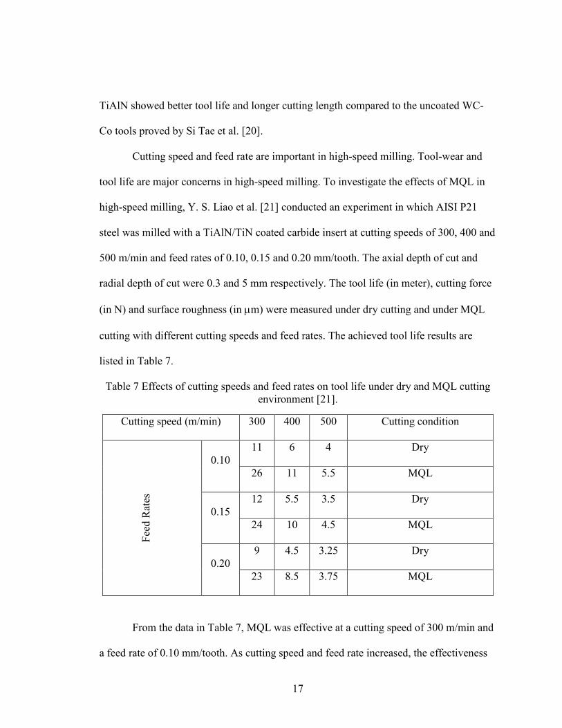
Cutting speed and feed rate are important in high-speed milling. Tool-wear and

tool life are major concerns in high-speed milling. To investigate the effects of MQL in

high-speed milling, Y. S. Liao et al. [21] conducted an experiment in which AISI P21

steel was milled with a TiAlN/TiN coated carbide insert at cutting speeds of 300, 400 and

500 m/min and feed rates of 0.10, 0.15 and 0.20 mm/tooth. The axial depth of cut and

radial depth of cut were 0.3 and 5 mm respectively. The tool life (in meter), cutting force

(in N) and surface roughness (in µm) were measured under dry cutting and under MQL

cutting with different cutting speeds and feed rates. The achieved tool life results are

listed in Table 7.

Table 7 Effects of cutting speeds and feed rates on tool life under dry and MQL cutting environment [21].

Cutting speed (m/min) 300 400 500 Cutting condition

Feed

Rat

es

0.10 11 6 4 Dry

26 11 5.5 MQL

0.15 12 5.5 3.5 Dry

24 10 4.5 MQL

0.20 9 4.5 3.25 Dry

23 8.5 3.75 MQL

From the data in Table 7, MQL was effective at a cutting speed of 300 m/min and

a feed rate of 0.10 mm/tooth. As cutting speed and feed rate increased, the effectiveness

18

of lubrication decreased. MQL seems to provide extra oxygen to chip-tool interface so as

to promote the formation of a protective layer of oxides. At optimal cutting speeds this

layer is stable and creates the barrier for diffusion, which aids in the wear resistance of

the cutting tool and increases the tool life significantly. At high cutting speed, the

formation of this layer becomes unstable and tool life decreases. Cutting force and

surface roughness were measured for different cutting speed when feed rate was 0.15

mm/tooth and depth of cut was o.3 mm, and are shown in Table 8. From the data shown

in Table 8, it can be said that cutting forces and surface roughness values were smaller

for MQL compared to dry cutting.

Table 8 Effects of cutting speeds on cutting force and surface roughness in dry and MQL cutting environment [22].

Cutting speed

(m/min)

Cutting force (N) Surface roughness (µm)

Dry MQL Dry MQL

300 47.5 44 0.21 0.16

400 46 44 0.20 0.16

500 45 43 0.19 0.15

The results in Table 8 indicate that MQL proved to be beneficial to tool life for

AISI D2 cold work steel in high-speed milling when WC-Co carbide was coated with

TiAlN/TiAlSiN [22].

In most of the turning and milling processes, a tool makes the contact on the outer

surface of the work piece. So the cutting temperature can be reduced easily. Chips can be

segmented and flown over the tool. But in drilling operation, it is difficult to reduce the

19

temperature when a drill cuts the material. The chip removal is also one of the concerns

during drilling operations. As drilling proceeds during machining, there is rubbing action

among the cutting edge of the tool, the machined surface and the chips. This results in

high temperature due to friction. It is necessary to decrease the temperature of the tool

and the work piece through an effective cooling system to achieve better tool life and

surface finish. Due to the high temperature, machined surface becomes less brittle and

rigid. There are more chances that both, tool material as well as the work piece material

diffuses into each other. Much research is done on machining AISI 1018 steel. In 2004,

Makiyama Tadashi et al. [23] conducted an experiment of drilling on 0.5% carbon steel.

Holes were drilled with a TiAlN coated solid carbide twist drill with a cutting speed of

120 m/min and a feed of 0.2 mm/rev. Holes were drilled under wet cutting, dry cutting

condition and minimum quantity lubrication (MQL). Ester oil was used in MQL with two

different flow rates of 5 ml/h and 10 ml/h. The air pressure was set at 0.5MPa in MQL.

The tool life and hole size deviation were measured to analyze the effect of MQL, flood

cooling and dry cutting condition. In dry cutting condition, tool life was found to be 31.7

m, (equivalent to 1554 holes). In wet cutting condition, tool life was found to be 61.1 m

(equivalent to 2995 holes). The tool life in MQL with 5 ml/h was found to be 78.3 m

(equivalent to 3838 holes) and with 10 ml/h, tool life was found to be 215.4 m

(equivalent to 10559 holes). The tool life was found maximum in MQL with a 10ml/h

flow rate. In dry cutting, the largest cutting torque was recorded with an irregular surface.

Hence, tool life was found to be the shortest. Wet cutting had the highest cooling effect

and smallest hole-diameter deviation. The MQL with 5ml/h flow rate had medium effect

20

of cooling and the largest enlargement of hole-diameter. The finished hole-surface had

regular feed marks without burnishing effect. That might be the reason for the lower

torque. MQL with 10ml/h flow rate had the largest tool life with larger enlargement of

drilled holes and had a smaller cutting torque. The results indicate that there is a

relationship between the enlargement of diameter of the drilled hole and tool life.

In 2005, Heinemann et al. [24] analyzed the effect of MQL on tool life of small

twist drills in deep-hole drilling. The study was done on 0.45% plain carbon steel. Four

types of drill were used: a) uncoated high speed steel (HSS), b) uncoated Co-HSS, c) TiN

coated Co-HSS and d) TiAlN multilayer-coated Co-HSS. Three different types mist were

used in MQL: SETOL ST-SHAD 20A (Synthetic ester + additives + alcohol 20%),

SETOL ST-SHAD (Synthetic ester + additives) and SETOL SOE (Oil free synthetic

lubricant + 40% water). The cutting speed was 26 m/min and the feed rate used was 0.26

mm/rev. The objective was to study the effect on tool life when MQL was to be applied

in continuous form and discontinuous form. The experiment was run further with

different kind of MQL. When drilling was carried out under continuous supply of MQL

with a flow rate of 18 ml/h, tool life (number of drilled holes) for different drills were as

follows: a) uncoated HSS drilled 558 holes, b) uncoated Co-HSS drilled 536 holes, c)

TiN coated Co-HSS drilled 709 holes and d) TiAlN coated HSS drilled 966 holes. When

MQL was applied discontinuously (MQL supply resumed during withdrawal after

drilling hole), tool life dropped drastically. Uncoated Co-HSS drilled only 13 holes (98%

drop), TiN coated Co-HSS drilled 411 holes (42% drops) and TiAlN coated Co-HSS

drilled 709 holes (27% drop). To see the effect of different MQL, experiment was run

21

again with uncoated HSS drill under 18ml/h flow rate of MQL. It was found that 558

holes were drilled with SETOL ST 20A lubricant, 689 holes were drilled with SETOL ST

SHAD lubricant and 1117 holes were drilled with SETOL SOE lubricant. It can be

concluded from the results that MQL with high cooling capability is advantageous for

deep-hole drilling.

In 2010, Shaikh and Boubekri [25] evaluated the performance of high-speed steel

(HSS) drill on AISI 1018 steel. The experiment was conducted on AISI 1018 steel work

pieces. With three different cutting speeds: 80, 100, and 120 SFM and two different feed

rates: 0.004 and 0.003 IPR. Aculube 6000 vegetable oil was used as MQL. The study was

conducted to measure the tool life of drill in terms of number of holes and surface finish

of the drilled hole. After collecting the hole-size of diameter and surface finish,

regression models were generated for both the inner diameter and the surface finish in

terms of cutting speed and feed rate. The tool life at different cutting speed and different

feed rate are shown on Table 9.

Table 9 Effect of cutting speeds and feed rates on tool life [25].

Cutting speed

(SFM) 80 100 120

Feed Rate (IPR) 0.003 880 490 530

0.004 430 390 280

It was observed that at lower feed rate (i.e. 0.003 IPR), as cutting speed increased,

the surface roughness of drilled hole also increased and for higher feed rate (i.e. 0.004

22

IPR), as cutting speed increased, the surface roughness was decreased [25].

Summary

From the literature review we can conclude that extensive research has been

conducted in machining steel. Most of the operations including turning, milling, drilling,

grinding and grooving are performed under MQL. Flood coolant machining failed to

reach at the tool-chip-work piece interface and hence cutting temperature was observed to

be high. In MQL, mist particles helped to reduce cutting temperatures, cutting forces and

surface roughness. In machining, tool material also plays an important role in achieving

a good tool life. It has been observed that tools having TiAlN/TiN coating improve the

tool life as these coatings improve heat resistance during machining. MQL was proved

more effective than flood cooling machining for speed ranging from 50 m/min to 130

m/min, feed rate ranging from 0.1 mm/rev to 0.2 mm/rev. MQL also proved to be better

for high speed turning and milling.

Problems observed during drilling operations were the removal of chips and the

high cutting temperatures. Due to the high temperature, tool life decreases with increases

in cutting forces, surface roughness and power consumption. Many experiments were

conducted with dry cutting (i.e. without the use of cutting fluid). The flood coolant

delivery technique helped to remove the chips from the drill hole but it was ineffective in

reducing the temperature of the tool-work piece interface. MQL system was more

effective than the flood cooling system, because a reduction in temperature was achieved

at the tool-work piece interface due to mist particles reaching this interface. The usage of

coated twist drill along with MQL cooling system provided better results for tool life,

23

tool wear and surface finish. The effectiveness of the MQL depends on the type of

lubrication used, cutting speed, feed rate, tool material, flow rate of MQL and air pressure

in MQL. A study in 2010 by Shaikh and Boubekri [25] on drilling 1018 steel explains the

effect of MQL with combination of different cutting speeds and feed rates. The effects

were measured in terms of tool life (number of holes drilled) and surface roughness (µm).

Tool life was decreased as cutting speed increased and surface roughness decreased when

cutting speed increased.

24

CHAPTER III

EXPERIMENTAL METHOD AND PROCEDURE

This chapter describes the experimental process and measurement procedure for

this research. It also describes the objective of the study, sample preparation, work piece,

machine tool and cutting tool descriptions and data analyses.

Objectives

The main objectives of this study are:

• To evaluate the performance (in terms of number of holes drilled) of uncoated HSS

twist drill when drilling AISI 1018 steel at cutting speeds of 80 and 120 SFM, feed

rates of 0.003 and 0.004 IPR using a newly developed lubricant designed for MQL

system. It is different lubricant than the lubricant used by Shaikh and Boubekri [25].

• To compare the study results with those obtained by Shaikh and Boubekri [25] when

AISI 1018 steel was drilled with uncoated HSS drill and Acculube 6000 vegetable oil

for mist.

• To characterize the tool wear using tool maker microscope.

Design of Experiments

The experiment was carried out with two independent variables: speed and feed

rate and one dependent variable, hole size. The experiment was carried out based on a

randomized factorial design. The hole-depth was one inch for entire drilling operation.

25

Four cutting speed and feed rate combinations were selected to determine the effects of

mist cooling on the tool life of the HSS twist drill. The designs of experiment treatments

are shown in Table 10. The speed and feed rates are in feet per minute (SFM) and inch

per revolution (IPR) respectively.

Table 10 Speed and feed rate combination.

Number of experiment 1 2 3 4

Combination of cutting

speed and feed rate

C1, F1

80,0.003

C1, F2

80,0.004

C2, F1

120,0.003

C2, F2

120,0.004

The experiment was randomly conducted. There were two levels of cutting speed:

80 SFM (C1) and 120 SFM (C2), and two levels of feed rate: 0.003 IPR (F1) and 0.004

IPR (F2). Based on these, four combinations of cutting speed and feed rate were

established. The experiment was conducted as follows:

1. Any one combination of the cutting speed and feed rate out of four was selected

randomly and inserted manually in CNC program.

2. Randomly work piece was selected from the stack and 30 holes were drilled in each

work piece until the twist drill failed as per the failure criteria

3. The hole-diameter was measured for every 10th, 20th and 30th hole

4. Once the tool was failed, replaced the failed tool with the new tool

5. Inserted new combination of the cutting speed and feed rate and continued the

process for all four combinations

26

Cutting Tool

The cutting tool used for the drilling operation was a solid straight shank drill

made of regular high-speed steel. It was ordered in a batch of 10 assuming that tools were

assumed to be identical. The tools were ordered from Guhring Inc. with following

specifications:

• Company: Guhring Inc.

• Part Number: 00205DIN 338R-N

• Tool Material: HSS

• Tool Diameter: 0.5in

• Tool Length: 5.944in

• Flute Length: 3.976in

• Drill type: Solid drill with straight shank

• Cutting point angle: 118°

Figure 4 HSS drill.

Coolant

Synthetic cutting fluid was used for mist generation along with compressed air.

27

“EQO-KUT 718” by QualiChem Inc. was used as a coolant. The properties of the fluid

were as follows:

• Appearance: Light yellow

• Density: 7.67 lbs/gal

• Flash point, COC: 360°F (180°C)

• Viscosity, SUS @ 100°F (38°C): 175

• Fat: Synthetic

• Chlorine and Active Sulfur: None

The cutting fluid was mixed with the compressed air in the unit called “Mister”

(Figure 5). The mister is attached outside of the machine. The mist was applied externally

on the cutting tool as shown in Figure 6. The air pressure was set to 0.15MPa. The

coolant flow rate was set to 12 ml/hr.

28

Figure 5 Mist lubrication unit.

Figure 6 Externally applied MQL.

Sample Preparation

Before starting the drilling experiment, the material was cut to make samples for

the experiment. The material was ordered from a local vendor. The four bars of 10 feet

length were cut using a band saw machine as shown in Figure 7. Because of the

limitation of clamping device in CNC machining center, the diameter of the work piece

was restricted to 4 inches. The samples were made as follows:

1. The bar was placed the roller bed of the band saw machine.

2. The bar was clamped tightly between the clamp and first cut of 0.5inch was made on

the bar to make the surface perpendicular to the bed.

29

3. If specified with the results of step 2 above, 1.75inch thick blanks were cut from the

bar and placed on the wooden pallet (Figure 8)

4. To transform 1.75inch thick blanks in to 1.5inch thick sample, the blanks were

processed in a CNC lathe machine for a facing operation on each surface.

5. The 1.75 inch blank was clamped in hydraulic operated chuck

6. During the facing operation on one surface, 0.075inch of material was removed from

that surface (Figure 9)

7. The processed blank was then clamped on opposite surface to process the other

surface

8. On this opposite surface, a total of 0.175inch material was removed in a similar

manner as done on the first surface of the blank (Figure 10)

9. On the same surface, the blank diameter was reduced to 3.950inch up to 0.75 inch in

length through a turning operation (Figure11).

10. A chamfering radius of 0.1659inch was machined on same side. The purpose of

reducing the diameter and chamfering was to locate and clamp the work piece

securely in a CNC machining center.

The first facing operation was done via one program and another facing, turning

and chamfering operation was via a second program in the CNC lathe. All the

unprocessed work pieces were kept on a wooden pallet near to the CNC machining

center.

30

Figure 7 Band saw cutting (Source: MFET Lab, UNT).

Figure 8 Blank from bar.

31

Figure 9 Facing on first face.

Figure 10 Facing on opposite surface.

32

Figure 11 Work piece for experiment.

Before the drilling experiment, a number of layouts were drawn on paper. The

layout selected was one in which a maximum number of holes were fitted. The program

was written and uploaded into the CNC machining center as per the selected layout. The

program was written for 30 holes of 1inch depth and 0.5 inch diameter. The pattern of the

hole was symmetric. To identify the first drilled hole, one slot was machined at an edge

of the work piece using an end mill cutter. Dry runs were conducted to check the program

correctness. The layout is shown in Figure 12. During dry runs, the position of nozzle for

mist application was set. The air pressure and coolant flow rate was set at the time of dry

runs only.

33

Figure 12 Work piece layouts.

34

Drilling Equipment

Figure 13 Drilling equipment (Source: MFET Lab, UNT).

Vertical machining center used to drill the holes. The machine specifications are as

follows:

• Machine make: Mori Seiki Dura Vertical 5060

• Controller: CNC Fanuc controller MSX-504 III

• Maximum Spindle speed: 10000 RPM

• Travel range in X-Axis: 23.600 inches

• Travel range in Y-Axis: 20.900 inches

• Travel range in Z-Axis: 20.100 inches

35

Work Piece Material

AISI 1018 was used as the work piece material. It has fair machinability, good

hardening properties and can be readily welded and brazed. This material is mostly used

for shaft, axel, sprocket assemblies, spindles, screw and bolts. The material is available in

cold rolled round, square, flat bar or hexagonal shape. Because of its hardening ability

and Manganese content, 42 RC-hardness can be achieved even in thin sections. The

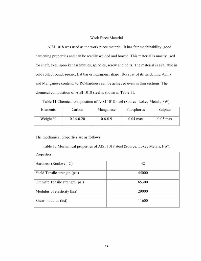
chemical composition of AISI 1018 steel is shown in Table 11.

Table 11 Chemical composition of AISI 1018 steel (Source: Lokey Metals, FW).

Elements Carbon Manganese Phosphorus Sulphur

Weight % 0.16-0.20 0.6-0.9 0.04 max 0.05 max

The mechanical properties are as follows:

Table 12 Mechanical properties of AISI 1018 steel (Source: Lokey Metals, FW).

Properties

Hardness (Rockwell C) 42

Yield Tensile strength (psi) 45000

Ultimate Tensile strength (psi) 65300

Modulus of elasticity (ksi) 29000

Shear modulus (ksi) 11600

36

Drilling Procedure

Before starting the drilling operation, check for:

1. The mist lubrication oil tank for the proper level of oil in the mist generator device.

(The device is attached to the backside of the machine.)

2. Check the air knob and the power supply switch.

Keep the pallet of all the previously machined samples near by the machine. Follow

the following steps.

1. Insert the control panel key and door keys

2. Turn on the machine by pressing the POWER ON button on control panel.

3. Select and insert the correct program. Select any one combination of cutting speed

and feed rate from the Table 10 and type in the selected program.

4. Check and make sure that all the values fed are correct in the program

5. Open the door of the machine by pressing DOOR OPEN button.

6. Clean the three jaw chuck with brush to remove the chips from the clamping area

7. Place the sample and tight the sample with the mallet and ensure that sample is

tightened enough.

8. Close the door of the machine

9. Press START button on control panel. Center drilling will start.

10. After completion of center drilling, machine stops because of the optional stop

command in program. Check visually for all center drilled holes.

11. Press START button for further drilling operation.

37

12. After drilling every three holes, machine stops because of optional stop. Open the

door and remove the accumulated chips from the drill as well as from the work piece.

13. Close the door and again press START button to continue drilling operation.

14. Repeat steps 13 and 14 till the program completion.

15. After completion of 30th hole, machine stops again and press START button again for

the milling process.

16. Open the door and with the help of the file, remove the burr from milled surface for

safety purpose.

17. Unclamp the work piece from the chuck with chuck-key and mallet.

18. Clean the work piece with compressed air to remove the accumulated chips and

coolant in the drilled holes

19. Measure the 1st hole with the help of digital vernier caliper and then measure every

10th, 20th and 30th hole of every work piece as per the inner diameter measuring

procedure.

20. Record all the values of each measurement in the spreadsheet.

21. Repeat steps from 7 to 21 until the tool fails as per the data collection method

Once the tool fails, remove the tool from ATC. Unclamp the tool from the tool

holder and clamp a new tool for the next combination of cutting speed and feed rate.

Before replacing the new tool clean the tool holder for coolant. Do the tool length

compensation1 for the new tool to make work piece top surface as a datum for the tool.

1 Tool length compensation steps are given in following page.

38

Repeat the same steps whenever the tool needs to be changed for all the combinations of

cutting speed and feed rate.

Tool length compensation steps for the new tool:

1. Clamp the work piece in the vice and the tool in tool holder

2. Bring the work piece under the tool axis manually

3. Bring the tool on the work piece surface manually

4. Maintain the gap of page thickness by inserting the page in between the work piece

and the tool

5. Record the value of Z-axis and insert the value in tool length compensation tab for Z-

axis

Data Collection Method

Tool is considered as failed when

• The reading of three consecutive holes is greater than or equal to 0.510 inches

or

• The reading of any hole is less than the first-hole reading.

Inner Diameter Measurement Procedure

1. Measure every 10th, 20th and 30th hole with digital vernier caliper. Record all the

readings in spreadsheet

2. If hole reading goes equal or greater than 0.510 inches, measure previous two

consecutive holes diameter. If all readings are greater than equal to 0.510 inches then

tool is considered to have failed.

39

3. If previous two holes readings do not repeat the condition of greater than equal to

0.510 inches then continue the drilling process for next 30 holes.

4. If hole-diameter reading is less than the first hole then the tool is considered as failed.

Data Analysis

After collecting all the data for hole-size, an analysis of Variance (ANOVA) was

conducted by using Design of Experiment-8 software. The purpose of ANOVA was to

determine if there was any significant difference in hole-size due to a specific

combination of cutting speed and feed rate. For ANOVA test, the independent variables

were cutting speeds and feed rates and dependent variable was hole-size. The following

steps were performed for ANOVA:

• Organize the data properly in spreadsheet for all combination readings

• Inspect the F-value, to determine if the model is significant

• Determine if the interaction and main effects for independent variables are significant

• Check R-squared value for the regression model. If required perform transformations

to get better values of R-squared

• Plot the required graphs

To characterize the tool wear, analyze all collected failed tools under the

toolmakers microscope. The value of flank wear is the distance between the peak and

valley on the flank edge of the tool as shown in Figure 14. Measure the flank wear on

both the edge of the tool and take the average value.

40

Figure 14 Flank wear measurement.

Tool Failure Analysis

All failed tools were analyzed for its failure pattern. The tools were observed

under toolmakers microscope. The flank wear and chipping areas were observed and

measured under 20X magnification lens. The photographs were taken using moticam

software.

Main Assumption of Study

• Drilling load had negligible effect on tool life

• Mixture of oil and compressed air and flow rate of mist was continuous

throughout the drilling operation

• Work piece samples are identical

• Cutting tool used are identical

41

• Procedure of hole-diameter measurement with digital vernier caliper was

consistence throughout the experiment

• ANOVA was the proper statistical tool to analyze the model

• Machine tool rigidity did not affect the tool life

• Only the numbers of hole drilled by the drill bit decided the tool life of drill

42

CHAPTER V

ANALYSIS

In this study, all collected data was recorded in a Microsoft excel file. This data

was then transferred to the Design Expert 8 statistical tool software for Analysis of

Variance (ANOVA) and regression analysis. The assumptions for the ANOVA are that

within each group, the individual measurements and associated residuals are normally

distributed, the groups compared should exhibit equal variance, and the individual

measurements and associated residuals in one group are independent from those found in

another group.

Hypothesis

The hypothesis tested is the following: Null Hypothesis:

There is no significant difference in the hole-diameters (responses) by changing the

cutting speed and feed rate combinations (input variables).

Alternative Hypothesis:

There is significant difference in the hole-diameters (responses) by changing the cutting

speed and feed rate combinations (input variables).

The diameters of the hole obtained from the drilling on AISI-1080 steel were

transferred into the Design Expert 8 software. To determine the suitability of the data for

43

ANOVA analysis, various graphs were plotted for this analysis (e.g., a normal plot of the

residual alone and a plot of the residuals versus the predicted values). The residual is the

difference between actual value of hole-diameter and predicted value of the hole-

diameter. In the analysis of variance plot, the normal probability distribution of residuals

is expected. The normal plot of the residuals is shown in Figure 15. A plot of the

internally normalized residuals versus the normal % probability approximates a straight

line, indicating normal distribution behavior of these normalized residuals. As the data is

normalized, the diameters of the hole can be said to be suitable for ANOVA analysis as

they follow a normal distribution.

Figure 15 Normal probability plot.

44

For the assumption of constant variance, the graph of residual versus predicted

value was obtained from the design of expert software. The graph of residuals vs.

predicted is shown in Figure 16. The graph shows equally distributed random behavior

about the centerline indicating constant variance.

Figure 16 Predicted vs. residual graph.

Table 13 shows the ANOVA results for hole-diameters based on the data obtained

from drilling. A two factor randomized factorial design was used for the analysis of

variance. In the table, term A is noted for the varying of cutting speeds group, term B is

noted for the varying of the feed rates group and term AB is noted for interaction between

45

cutting speeds and feed rates. ANOVA table contains sources, sum of squares, degree of

freedom (df), mean square and p-value. The model F-value of 340.18 implies the model

is significant. There is only a 0.01% chance that a “Model F-Value” could be large due

to noise. The ANOVA indicates that there is a significant difference between the two

groups A and B. Values of “Prob > F’ less than 0.0500 indicate that A and B terms are

significant. Values greater than 0.1000 indicate that A and B are not significant. The

software regression results indicate that the variables A, B, and AB interaction are

significant and thus have an effect on the surface diameter of the hole.

Table 13 ANOVA analysis table for hole-diameter.

46

As mentioned before, the software also shows the linear regression results for the

data used in the ANOVA. The R-Squared value is the value, which shows how well the

data fits the linear regression model. Its value lies between 0 and 1. The value towards 1

indicates a perfect fit for the linear regression model. There are many variations in the

process like human error, cutting forces, material variation, coolant flow and measuring

error that can prevent the data from fitting the model perfectly. The R-squared value for

the selected regression model of surface diameter hole size is 0.7847. It means that this

regression model is able to predict 78.47 percent variations in the process. The remaining

21.53 percent is unaccounted for. The predicted R-Squared value measures how well the

regression model is predict the response value. The adjusted R-Squared value measures

the amount of variations from the mean. The values of predicted R-squared value and

adjusted R-Squared value for the hole-diameter are 77.86 percent and 78.24 percent

respectively. The table also shows the value of “Adequate Precision”. It measures the

ratio of the signal to noise. The ratio value greater than 4 is always good. For this model,

Adequate Precision value is 41.998 hence this model can be used to navigate the design

space.

The regression equation obtained is:

Hole Diameter = 0.51 + (2.310E-004 X Cutting speed) + (1.251E-003 X Feed rate) –

(8.896E-004 X Cutting speed X Feed rate)

47

Correlation Analysis

A plot between hole-diameter versus number of hole drilled for combination of

the cutting speed of 80 SFM and the feed rate of 0.003 IPR is shown in Figure 17. It was

observed that there is increase in diameter size from 0.5020 inches to 0.5052 inches up to

hole-number 360. There was a sudden fall in hole-size from 0.5052 inches to 0.5022

inches. The chipping off might have caused this from flank surface of the tool. Figure 18

and Figure 19 shows the trend line for first 100 holes and the last 100 holes drilled. For

the first hundred holes, diameter was increased and hence the trend line was in the

upward direction. For last hundred holes, the diameter size was decreased from 0.5032

inches to 0.5018 inches, resulting in downward trend line. The tool life was 1110 holes

for the combination of 80 SFM cutting speed and 0.003 IPR feed rate. The diameter for

1st hole was measured as 0.5020 inches. The diameter for 1120th hole was 0.5018 inches,

which was less than the first hole and at this occurrence; the tool was declared as having

failed.

Figure 17 Hole-diameter vs. number of holes (80SFM, 0.003IPR).

48

Figure 18 Hole-diameter for first hundred holes (80SFM, 0.003IPR).

Figure 19 Hole-diameter for last hundred holes (80SFM, 0.003IPR).

49

When X, the number of holes, was plotted against Y, the diameter of the holes, an

attempt was made to determine the linear equation that best fits the data for the following

groups. The overall gathered data for a combination, the first hundred holes for a

combination and the last hundred holes for a combination. For the first combination,

Table 14 lists the results.

Table 14 Coefficient of correlation for the Combination 1.

Equation Coefficient of correlation

For over all data Y= 0.5033 – 3*10-7X -0.1183

For first hundred holes Y= 0.5024 – 9*10-6X 0.4107

For last hundred holes Y= 0.5016 – 1*10-5X -0.2350

From the Table 14, it is observed that the coefficient of correlation for the first

hundred holes is positive and for the last hundred holes it is negative. The overall

correlation coefficient is negative. The coefficient of correlation -0.118 indicates a slight

negative correlation exists between the variables diameter of the holes and the number of

holes. If coefficient of correlation is -1.0 then there is a perfect negative correlation

between these two variables. When one variable increases, another variable decreases. If

the coefficient of correlation is 0, there is no correlation between these two variables. If

the coefficient of correlation is 1.0, there is a perfect positive correlation between these

two variables. When one variable increases, another variable increases too. When one

variable decreases, the other variable decreases too.

50

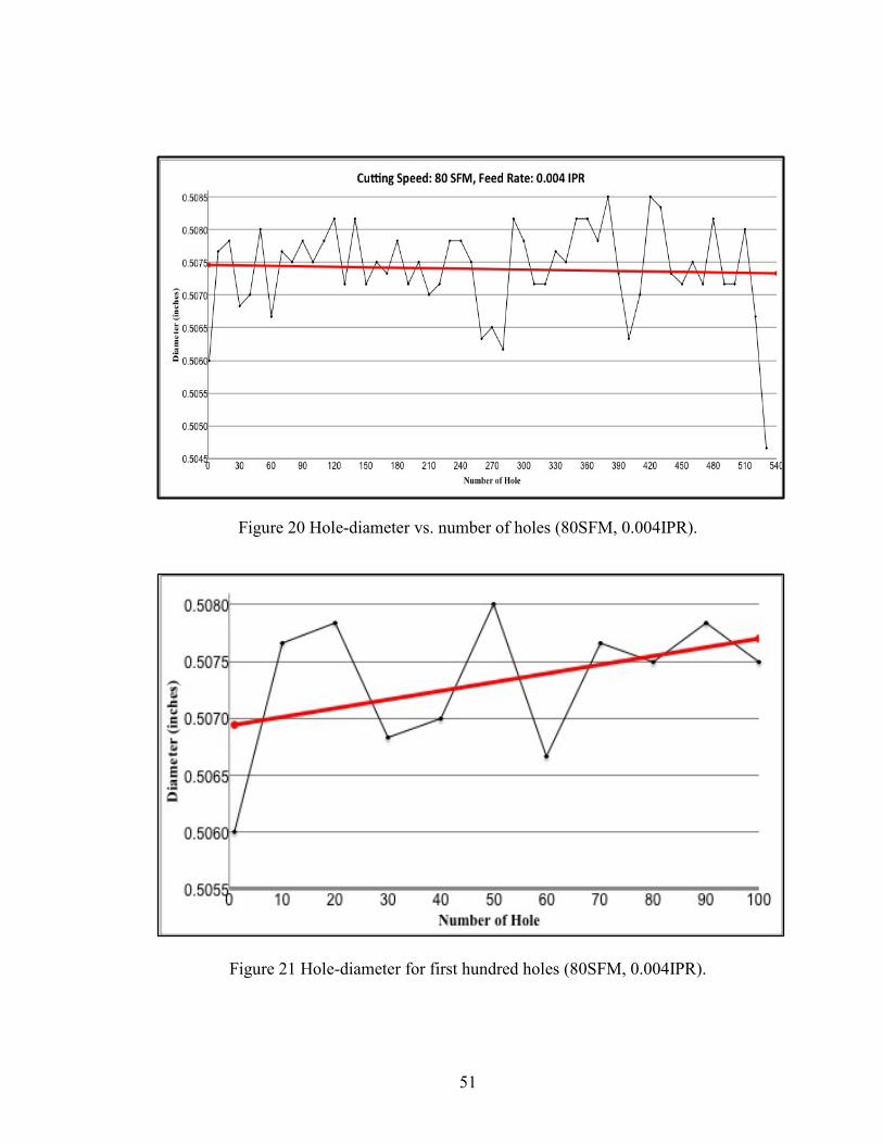
The correlation analysis for the combination of another cutting speed and feed

rate is shown in Figure 20. The cutting speed was the same, 80 SFM, but the feed rate

was increased from 0.003 IPR to 0.004 IPR. The maximum number of holes drilled with

this combination was 530. The hole-diameter for the first hole was recorded as 0.5060

inches. The value for 530th hole was 0.5047 inches, which was less than first hole and

hence the tool was declared as failed. Compared to the first combination, the tool life

here was less for the second combination. Due to the higher feed rate, the cutting force

and the cutting temperature might be higher here, which may have shortened the life of

the tool. The trends for first hundred and last hundred hole-diameters are shown in Figure

21 and 22, respectively. For last hundred holes, the data shows a sudden fall in hole-

diameter from 0.5085 inches to 0.5047 inches. This indicates that the diameter being

reduced may be due to flank wear or crater wears on the tool surface. The wear on tool

surface can be investigated under toolmakers microscope. The largest hole-diameter in

this combination was recorded to be 0.5087 inches.

51



52


For the second combination, an attempt to fit X, the number of holes to Y, the

diameter of holes, in a linear model resulted in values listed in Table 15.






From the Table 15 shows the equations and coefficient of correlation for over all

data, the first hundred holes and the last hundred holes for the second combination. The

correlation is not strong correlation for over all data.

53

In the third combination, the maximum cutting speed of 120 SFM and minimum

feed rate of 0.003 IPR was used. The tool lasted up to 870 holes. The maximum diameter

measured here was for hole-number 580. The hole-diameter here was 0.5083 inches. It

was observed from Figure 23, the diameter did not vary much up to 400 holes. After that,

the hole-diameter reached maximum and tool failed on hole-number 870. The diameter

for hole-number 870 was measured 0.5028 inches. Compare to the combination of the

lowest cutting speed and highest feed rate i.e. 80 SFM and 0.004 IPR; this combination

has more tool life. The correlation for first hundred and last hundred is shown in Figure

24 and 25, respectively. The hole-diameter increased from 0.5038 inches to 0.5063 inches

for the first hundred holes and for the last hundred holes, hole- size decreased from

0.5048 inches to 0.5028 inches. The correlation coefficient values for the third

combination are shown in Table 16.

23 Hole-diameter vs. number of holes (120SFM, 0.003IPR).

54



55

For the third combination, an attempt to fit X, number of holes to Y, the diameter

of holes, in a linear model resulted in values listed in Table 16.






The correlation for the overall data is negative. For the first hundred holes

correlation is positive between the number of holes and hole-diameter. The proposed

linear equations are not a good fit for this data.

The correlation analysis for last combination of cutting speed and feed rate is

shown in Figure 26. With this combination, a total of 290 holes were drilled. The

maximum hole-diameter measured was 0.5078 inches. There was overall variation found

in the hole-diameters. In this combination, maximum cutting speed and maximum feed

rate was used to drill the holes. Due to higher feed rate, cutting forces and temperature

might be higher in cutting zone. The flank wears or crater wear was quickly and tool

failed quickly. No particular pattern was observed in hole-diameter over the number of

hole. The correlation analysis for first hundred holes and last hundred holes is shown in

Figure 27 and 28, respectively. The trend of hole-diameter in the first hundred holes is

increasing and for last hundred holes is decreasing. The hole-size for 290th hole, 0.5040

inches was smaller than first hole, 0.5043 inches, which indicated failure of the tool.

56



57


For the last combination, an attempt to fit a linear model to X, the number of

holes, to Y, the diameter of holes resulted in Table 17 values.






Table 17 shows the equations and coefficient of correlation for the fourth

combination. The correlation for over all data and for last hundred holes is negative. For

the first hundred holes, correlation is positive. The proposed linear models are not a good

fit for any of the data sets.

58

Tool Life Analysis

The tool life comparison is shown in Figure 29. The effect of feed rate on tool life

is ploted on the graph for different cutting speeds. It is observed that tool life with lower

feed rate and lower cutting speed was maximum. For cutting speed 80 SFM and

0.003IPR feed rate, tool life was 1110 holes. If the feed rate was increased from 0.003 to

0.004 IPR, the tool life was decreased from 1110 holes to 520 holes and that was equal to

a 53% reduction in tool life. For 120 SFM cutting speed tool life was 860 holes for 0.003

IPR. Increasing the feed rate from 0.003 IPR to 0.004 IPR, keeping cutting speed at 120

SFM, the tool life was reduced from 860 holes to 280 holes which was equal to 67%

reduction in tool life. The tool life was reduced drastically in combination of higher feed

rate and higher cutting speed.

Figure 29 Feed-rate vs. tool life.

1110

520

860

280 200

400

600

800

1000

1200

0.0025 0.003 0.0035 0.004 0.0045

Tool

Lof

e (N

umbe

r of

dri

lled

hole

s)

Feed Rate

Effect of Feed Rate on Tool Life

80 SFM

120 SFM

80 SFM

120 SFM

59

The following Figure 30 shows the relation of tool life based on cutting speeds for

different feed rates. At lower cutting speed the tool life was 1110 holes for 0.003 IPR. It

was observed that increasing cutting speed from 80 IPR to 120 IPR, tool life was

decreased from 1110 holes to 860 holes, which was equal to 22.5% reduction. With

higher feed rate, tool life was lesser than lower feed rate. Tool life of 520 holes was

observed when drilling was done with 80 SFM cutting speed and 0.004 IPR. When

cutting speed was increased from 80 SFM to 120 IPR, tool life was reduced from 520

holes to 280 holes, which was equal to 46% reduction. Tool life was higher at lower

cutting speed compared to higher cutting speed.

Figure 30 Cutting speed vs. tool life.

1110

520

860

280

0

200

400

600

800

1000

1200

70 80 90 100 110 120 130

Tool

Life

(Num

ber

of D

rille

d H

oles

)

Cutting Speed (SFM)

Effect of Cutting Speed on Tool Life

0.003 IPR

0.004 IPR

0.003 IPR

0.004 IPR

60

The following Figure 31 shows the graph of tool life obtained by using two

different type of mist lubricator: one EQO-KUT 718 and Aculube 6000 vegetable oil

[25]. The tool life was compared for all four combinations of cutting speed and feed rate.

Figure 31 Tool-life for different mist lubrication.

It was observed that tool life obtained using EQO-KUT 718 was greater than tool

life obtained using Aculube 6000 mist lubrication oil. The combination of lower feed

rate with both the cutting speeds (i.e. 80 SFM and 120 SFM) caused the tool life to be

increased by 26% and 62% respectively by using EQO-KUT 718 oil. There was not

significant difference in tool life at higher feed rate and cutting speeds.

1110

520

860

280

880

430 530

280

0

200

400

600

800

1000

1200

80, 0.003 80, 0.004 120, 0.003 120, 0.004

Tool

Life

(Num

ber

of D

rille

d H

oles

)

Cutting Speed and Feed Rate Combination

Tool Life comparison based on Mist

Eco-Kut 718

Aculube 6000

61

Tool Failure Analysis

All failed tools were analyzed for the flank-wear or crater-wear. A toolmaker

microscope was used to analyze the tool. Failed drills were observed under 20X

magnification lens. The flank edges were analyzed and pictures were recorded with a

moticam camera attached on a microscope. The images were captured on computer.

It was observed that the drill, which was used to drill in combination of 80 SFM

and 0.003 IPR has flank wear of 0.058 mm. The material was removed slowly from the

flank edge during machining. No chipping was observed on the flank edge. Only gradual

wear was observed and this could be because the cutting speed as well as the feed rate

was low.

Figure 32 Tool-failure for first combination.

62

The tool failure for second combination was shown in Figure 33. On the flank

edge, flank wears and chipping were observed. Because of higher feed rate i.e. 0.004 IPR,

material from flank edge was chipped off and the tool had failed earlier compared to first

combination (cutting speed 80 SFM and feed rate 0.003 IPR). Due to the higher feed

rate, temperature as well as cutting forces was probably higher. The flank wear was

measured as 0.040 mm.

Figure 33 Tool-failure for second combination.

63

For the third combination i.e. higher speed of 120 SFM and lower feed of 0.003

IPR, the flank wear was noted about 0.06 mm. When the tool was observed under a

toolmakers microscope, the flank wear was observed on flank edges (this could have

been attributed to high cutting speeds). The material was also chipped off. Because of it,

the tool failed quickly. The flank wears and crater wear was shown in Figure 34 and 35.

In the fourth combination, the tool failed due to crater wear. The flank wear was less than

the crater wears. This wear could be because of higher cutting speed and feed rate which

could indicate high cutting forces and lower cooling effects compared to the other three

combinations. The failure was shown in Figure 36. The flank wear was noted as 0.034

mm.

Figure 34 Tool-failure for third combination-a.

64

Figure 35 Tool-failure for third combination- b.

Figure 36 Tool-failure for fourth combination.

65

Summary

The experiment of drilling in AISI 1018 steel was done with two different cutting

speeds: 80 SFM and 120 SFM and two different feed rate: 0.003 IPR and 0.004 IPR. The

drilling operation was done with four combinations of cutting speeds and feed rates. The

hole-diameter was measured each time after the tenth hole drilled. The hole-diameter

readings were analyzed in Design Expert-8 statistical software version for ANOVA. The

correlation analysis was done using excel.

For the combination of 80 SFM cutting speed and 0.003 IPR feed rate, tool life

was 1110 holes. The first hole-size was measured as 0.5020 inches. The maximum hole-

diameter recorded as 0.5052 inches for 360th hole. The hole-diameter for 1120th hole was

measured as 0.5018 inches, which was less than the first hole-diameter and based on this,

the tool was declared as having failed. For this combination, an increasing trend was

observed in hole-diameter and as machining was continued and a decreasing trend was

noted in the last hundred holes. When failed tool was analyzed under toolmaker’s

microscope, more flank wear was observed on the flank edges. The average flank wear of

0.058mm was measured.

For the combination of lower speed and higher feed rate i.e. 80 SFM and 0.004

IPR, the tool life of 520 holes was observed. The hole-diameter for the first hole was

0.5060 inches measured. Because of higher feed rate, tool life was lesser than the first

combination. The flank wears and crater wear were observed on the cutting edge of the

tool. The maximum hole-diameter was measured about 0.5085 inches for 380th hole.

66

When drilling was done with the third combination, cutting speed was set at 120

SFM and feed rate was set at 0.003 IPR. The tool life for this combination was recorded

as 860 holes. This combination was better than the second combination but lesser than

first combination. The hole-diameter for the first hole was measured as 0.5038 inches.

The maximum hole-size of 0.5085 inches was recorded for 580th hole. The hole diameter

for 870th hole was measured lesser than the first hole i.e. 0.5028 inches and thus, the tool

was declared as having failed as per the failure criteria set for the experiment. The

average flank wears of 0.060 mm was measured with toolmaker’s microscope.

The tool life for fourth combination was measured as 280 holes. In this

combination, drilling operation was done with maximum cutting speed of 120 SFM and

maximum feed rate of 0.004 IPR. With this combination, less tool life was observed in

the experiment. The hole-size for the first hole was measured as 0.5043 inches and

0.5040 inches for 290th hole. The maximum hole-diameter of 0.5078 inches was

measured for 60th, 110th and 160th hole. The crater wear was noticed more than the flank

wear on the failed tool.

It was observed that for the lowest combination of the cutting speed and the feed

rate: 80 SFM and 0.003IPR respectively, the tool life and flank wear on the tool was

maximum: 1110 holes and 0.058mm respectively. For the highest combination of the

cutting speed and the feed rate: 120 SFM and 0.004 IPR respectively, the tool life and

flank wear on the tool was minimum: 280 holes and 0.034mm respectively.

When the tool life was compared based on the mist lubrication oil used, it was

observed that the tool life using EQO-KUT 718 was more than the tool life using

67

Aculube 6000. For the fourth combination, tool life was same for both the mist

lubrication oil. For first combination, the tool life was 26% more for EQO-KUT 718 than

Aculube 6000. For the third combination the tool life was increased by 62% for EQO-

KUT 718 mist lubrication oil.

68

CHAPTER VI

CONCLUSION

The experiment was conducted to analyze the effect of mist lubrication on AISI

1018 steel by comparing the tool life based on the lubrication used. The machining was

done with four combination of cutting speed and feed rate. Two cutting speeds: 80 SFM

and 120 SFM and two feed rates: 0.003 IPR and 0.004 IPR were used. The drilling was

done in 3 axes CNC machining center- Mori Seiki. EQO-KUT 718- lubrication oil was

used. It was applied externally. The hole-diameter was measured for all the samples and

gathered for data analysis. The conclusions were made as follows:

The maximum tool life of 1110 holes was realized using a cutting speed of 80

SFM and a feed rate of 0.003 IPR. When using cutting speed of 120 SFM and 0.003 IPR

feed rate, 860 holes tool life was recorded, was less than the first combination. This might

be because of possible excessive heat generated at the cutting zone and higher cutting

forces resulting in wear and tear of the cutting tool. The flank wear was noticed on the

cutting edge and chipping was minor at this combination.

The minimum tool life of 280 holes at a cutting speed of 120 SFM and a feed rate

of 0.004 IPR. Because of the higher cutting speed and feed rates, it is hypothesized that

there was increase in cutting forces, temperature and wear. As feed rate and cutting speed

increased, the cutting edge of tool got blunt which increased friction between tool and

work piece. Due to friction cutting temperature increased and tool life decreased.

69

The ANOVA was conducted based on the hole-size, cutting speed and feed rates.

The regression equation indicates that cutting speed, feed rate and the combination of

these two are all significant factors based on 95% confidence level. Therefore, the null

hypothesis- “There is no significant difference in the hole-size (responses) by changing

the cutting speed and feed rate combination (input variables)” is rejected.

Based on the results of this study and those obtained by Vasim and Boubekri [25],

the EQO-KUT 718 lubricant is more effective than the Aculube 6000 when drilling was

conducted at lower feed rates.

Recommendations for Future Research

Using other possible feed rates and cutting speeds levels, this experiment could be

extended. Alternatively, the same experiment could be repeated by drilling into another

commonly used metal or by changing to a different type of coolant to determine the tool

life or an affectivity of MQL. Other variables in the drilling procedure could be assessed

in future research. One of them could be evaluating the temperature variable during

cutting. With a laser temperature meter, the temperature effect while cutting could be

observed and recorded while cutting. This may lead to a better explanation on how the

temperature affects the wear and tear of the tool. This temperature effect could be

assessed with and without using a coolant.

Lastly, another possibility is to determine how the strain experienced in the tool

during drilling. Also, in this same case, a different measurement of tool life (in terms of

strain) could be used and this measurement could also be related to the hole-diameter.

70

REFERENCES

[1] Master Chemical Corporation, “Fluid application- MQL (Minimum Quantity

Lubrication).” Trim Technology Bulletin.

http://www.masterchemical.com/db-docs/technical-bulletins/Fluid_MQL.pdf

[2] Ron Quaile, et al. “Understanding MQL: Machining with minimum quantity lubricant

can save money and improve both tool life and part finish.” Modern Machine

Shop, (April 2011).

[3] Stephenson, David A. Agapiou, John S. “Metal cutting theory and practice.” Taylor

and Francis, 2006.

[4] Boelkins, Chuck. Unist. “MQL: Lean and Green.” Cutting Tool Engineering 61, no. 3

(March 2009): 71-75.

[5] Dhiman, Suresh, et al. “Machining behavior of AISI 1018 steel during turning.”

Journal of Scientific & Industrial Research 67, (May 2008): 355-360.

[6] Sun J., et al. “Effects of coolant supply methods and cutting conditions on tool life in

end milling titanium alloy.” Machining Science and Technology10, (2006): 355-

370.

[7] Zhao W., et al. “High speed milling of Ti6Al4V alloy with Minimal Quantity

Lubrication.” Key Engineering Material 329, (2007): 663-668.

71

[8] Obikawaa, Toshiyuki, et al. “High-speed grooving with applying MQL.” International

Journal of Machine Tools & Manufacturer 46, (January 2006): 1854-1861.

[9] Dhar, N. R., et al. “Effect of minimum quantity lubrication (MQL) on tool wear and

surface roughness in turning AISI-4340 steel.” Journal of Materials Processing

Technology 172, (2006): 299-304.

[10] Attanasio, A., et al. “Minimal quantity lubrication in turning: Effect on tool wear.”

Wear 260, (2005): 333-338.

[11] Dhar, N. R., et al. “The influence of minimum quantity lubrication (MQL) on cutting

temperature, chip and dimensional accuracy in turning AISI-1040 steel.” Journal

of Materials Processing Technology 171 (2006): 93-99.

[12] Dhar, N. R., et al. “An experimental investigation on effect of minimum quantity

lubrication in machining AISI 1040 steel.” International Journal of Machine tools

& Manufacture 47, (2007): 748-753.

[13] Khan, M. M. A., et al. “Performance evaluation of minimum quantity lubrication by

vegetable oil in terms of cutting force, cutting zone temperature, tool wear, job

dimension and surface finish in turning AISI-1060 steel.” Journal of Zhejiang

University SCIENCE A 7, no. 11(2006): 1790-1799.

[14] Ueda, Takashi, et al. “Effect of oil mist on tool temperature in cutting.” Journal of

manufacturing science and engineering 128, (February 2006): 130-135.

[15] Venkatesh, V. C., et al. “A study of chip surface characteristics during the

machining of steel.” Annals of CIRP 42, no. 1 (1993): 631-636.

72

[16] Jayal1, Anshu D., et al. “Effects of cutting fluid application on tool wear in

machining: Interactions with tool-coatings and tool surface features.” Wear 267,

(2009): 1723-1730.

[17] Khan, M. M. A., et al. “Effects of minimum quantity lubrication on turning AISI

9310 alloy steel using vegetable oil-based cutting fluid.” Journal of Material

Processing Technology 209, (2009): 5573-5583.

[18] Saluena-Berna, X., et al. “Analysis of the behavior effect of face cutting edge inserts

on surface roughness when milling steels with MQL lubrication.” Material

Science Forum 526, (2006): 25-30.

[19] Iqbal, Asif, et al. “Influence of cutter’s helix angle, work piece hardness, milling

orientation, and MQL in high-speed side milling if AISI D2.” Material Science

Forum 532-533, (2006): 45-48.

[20] Won, Si Tae, et al. “Measurement of TiAlN coating effects on machining

characteristics of high hardened steel.” Key Engineering Materials 321-323,

(2006): 1357-1359.

[21] Liao, Y. S., et al. “Mechanism of minimum quantity lubrication in high-speed

milling of hardened steel.” International Journal of Machine Tool & Manufacture

47, (2007): 1660-1666.

[22] Kang, M. C., et al. “Effect of the minimum quantity lubrication in high-speed end-

milling of AISI D2 cold-worked die steel (62 HRC) by coated carbide tools.”

Surface Coating Technology 202, (2008): 5621-5624.

73

[23] Tadashi, Makiyama, et al. “Drilling with MQL process.” 7Th International

Conference on Progress of Machining Technology, (2004): 169-174.

[24] Heinemann, R., et al. “Effect of MQL on the tool life of small twist drills in deep-

hole drilling.” International Journal of Machine Tool & Manufacture 46, (2006):

1-6.

[25] Shaikh, Vasim, et al. “Effect of effect of minimum quantity lubrication in drilling

1018 steel.” Journal of Manufacturing Technology Research 2, no. 2 (2010): 31-

44.

[26] McClure, T. F., et al. “Comparison of flood vs. micro-lubrication on machining

performance (Part 1).” Techsolve (Unist- Micro-fluidization products for

industry), (2007): 1-5. Www.unist.com/pdfs/articles/AR_flood_v_micro.pdf

[27] “Tool Spray.” Cutting Tool Engineering 60, no. 3 (2008).

Effects of minimum quantity lubrication (MQL) on tool …/67531/metadc149638/m2/1/high...Maru,...

Documents

Transcript of Effects of minimum quantity lubrication (MQL) on tool …/67531/metadc149638/m2/1/high...Maru,...