Effects of Love Waves on Microtremer HV Ratio

Effects of Love Waves on Microtremor H/V Ratio

by Sylvette Bonnefoy-Claudet, Andreas Köhler, Cécile Cornou, Marc Wathelet,and Pierre-Yves Bard

Abstract The horizontal-to-vertical (H/V) method has the potential to significantlycontribute to site effects evaluation, in particular in urban areas. Within the Europeanproject, site effects assessment using ambient excitations (SESAME), we investigatedthe nature of ambient seismic noise in order to assess the reliability of this method.Through 1D seismic noise modeling, we simulated ambient noise for a set of varioushorizontally stratified structures by computing efficiently the displacement and stressof dynamic Green’s functions for a viscoelastic-layered half-space. We performed ar-ray analysis using the conventional semblance-based frequence-wavenumber methodand the three-component modified spatial autocorrelation method on both vertical andhorizontal components and estimated the contribution of different seismic waves(body/surface waves, Rayleigh/Love waves) at the H/V peak frequency. We show thatthe very common assumption that almost all the ambient noise energy would be car-ried by fundamental-mode Rayleigh waves is not justified. The relative proportion ofdifferent wave types depends on site conditions, and especially on the impedance con-trast. For the 1D horizontally layered structures presented here, the H/V peak fre-quency always provides a good estimate of the fundamental resonance frequencywhatever the H/V peak origin (Rayleigh wave ellipticity, Airy phase of Love waves,S-wave resonance). We also infer that the relative proportion of Love waves in ambientnoise controls the amplitude of the H/V peak.

Introduction

The horizontal-to-vertical (H/V) spectral ratio (i.e., theratio between the Fourier amplitude spectra of the horizontaland the vertical component of microtremors) was first intro-duced by Nogoshi and Igarashi (1971), and was spreadwidely by Nakamura (1989, 1996, 2000). These authorspointed out the correlation between the H/V peak frequencyand the fundamental resonance frequency of the site and pro-posed to use the H/V technique as an indicator of the under-ground structure features. A large number of experiments(Lermo and Chavez-Garcia, 1993; Gitterman et al., 1996;Seekins et al., 1996; Fäh, 1997), supported by several theo-retical 1D investigations (Field and Jacob, 1993; Lachet andBard, 1994; Lermo and Chavez-Garcia, 1994; Wakamatsuand Yasui, 1996; Tokeshi and Sugimura, 1998; Bonnefoy-Claudet, Cornou, et al., 2006), has shown that noise syn-thetics computed using randomly distributed near-surfacesources lead to H/V ratios sharply peaked around the funda-mental resonance frequency of SH waves whenever the sur-face layer exhibits a sharp impedance contrast with theunderlying stiffer formations. However, the theoretical basisof the H/V technique is still unclear as two opposite explana-tions have been proposed. Nakamura (1989, 2000) claimsthat the H/V spectral ratio peak, by removing effects of sur-face waves, provides the S-wave resonance in the soft surface

layer, leading to H/V curves providing a consistent estimateof the site amplification. This body-wave interpretation hasbeen contradicted in several articles highlighting the relation-ship between the H/V and the ellipticity of fundamentalRayleigh-wave mode (Lachet and Bard, 1994; Kudo,1995; Bard, 1998; Fäh et al., 2001; Bonnefoy-Claudet,Cornou, et al., 2006) and thus has seriously questionedthe existence of any simple direct correlation between H/Vpeak value and the actual site amplification. Recently,Bonnefoy-Claudet, Cotton, et al. (2006) highlighted the lim-ited knowledge within the scientific community on the rela-tive contribution of body and surface waves to the actualambient noise wave field.

The goal of the present article is to investigate the rela-tionship between the ambient noise wave-field nature andcomposition and the effectiveness of the H/V method to es-timate site response parameters (resonance frequency andamplification factor). We simulate seismic ambient noisefor a set of various realistic horizontally stratified structures,perform array analysis using the conventional semblance-based frequency-wavenumber method (CVFK) and thethree-component modified spatial autocorrelation method(3C-MSPAC) on both vertical and horizontal components,and finally estimate the contribution of different seismic

288

Bulletin of the Seismological Society of America, Vol. 98, No. 1, pp. 288–300, February 2008, doi: 10.1785/0120070063

waves (body/surface waves, Rayleigh/Love waves) at theH/V peak frequency.

Noise Data Sets

Ten horizontally stratified structures consisting of vari-ous sedimentary layers overlying half-space, characterizedmainly by their impedance contrast, have been selected. Ta-ble 1 details the soil profiles used, which have been selectedto be as close as possible to actual soil properties. A nonex-haustive review of soil properties performed at 136 differentsites shows indeed that the soil structures considered in thisarticle are consistent with actual distribution of the S-wavevelocity contrast observed at those sites (Fig. 1). Moreover,attenuation values have been selected to model values typi-cally observed or considered for sedimentary deposits(Hauksson et al., 1987; Fukushima et al., 1992; Wang et al.,1994; Jongmans et al., 1998; Di Giulio et al., 2003).

The seismic noise recorded in urban areas (culturalnoise) can be considered as mainly caused by human activity(people walking, cars, factories, etc.) and propagates mainlyas high-frequency surface waves (>1 Hz) that attenuatewithin several kilometers in distance and depth (McMamaraand Buland, 2004; Bonnefoy-Claudet, Cotton, et al., 2006).

In our simulations, we do not take into account the effectof oceanic waves, which propagate over large distances inthe low-frequency range (i.e., ≪1 Hz). Except for thedeepest model (M3.3), where the resonance frequency is0.45 Hz, the resonance frequency of each site is large enoughnot to be influenced by propagation of such low-frequency waves.

Recently, Bonnefoy-Claudet, Cornou, et al. (2006)showed that at a given observation site, local and near-surface sources dominate the cultural ambient noise wavefield. Therefore we set up a source location to fulfill theseconditions. Spatial locations of sources and receivers are ex-pressed in a grid step the size of which varies according to thesedimentary layer thickness. The grid step is then set to 2 mfor the shallow model (M2.4), to 4 m for intermediate thick-ness models (M2.2, M3.1, M3.2, M4.1, M4.2, M4.3, andM4.4), to 8 m and 16 m for deep models (M2.3 andM3.3, respectively). 333 sources are randomly distributedin space and time. The maximum distance between the cen-tral receiver and sources is 361 grid step (Fig. 2a) and thedepth of the sources is 0.5 grid step. The minimum and maxi-mum distances between two receivers are 1 and 40 grid steps,respectively (Fig. 2b).

Table 1Soil Profiles Considered for the 1D Horizontally Layered Models

Model N H, (m) α (m=sec) β (m=sec) ρ (g=cm3) Qp Qs Zc Zv Fo Fell Fa

M2.2 2 25 1350 200 1.9 50 25 6.6 5 1.95 1.93 2.1— 2000 1000 2.5 100 50

M2.3 2 83 1350 667 1.9 50 25 2.0 1.5 1.94 - 3.3— 2000 1000 2.5 100 50

M2.4 2 10 1350 200 1.9 20 10 6.6 5 4.83 4.83 5.2— 2000 1000 2.5 100 50

M3.1 3 18 1350 250 1.9 50 25 4.6 3.5 2.11 2.15 2.318 1350 330 1.9 50 25

— 2000 1000 2.5 100 50

M3.2 3 18 1350 250 1.9 50 25 5.5 4.2 2.94 2.76 3.118 1350 625 1.9 50 25

— 2000 1500 2.5 100 50

M3.3 3 31.25 500 250 1.9 50 25 4.0 3.0 0.45 0.73 -375 1800 750 2.1 100 50

— 3500 2000 2.5 200 100

M4.1 2 36 1350 250� 2z 1.9 50 25 4.7 3.6 2 2 2.3— 2000 1000 2.5 100 50

M4.2 2 36 1350 250� 5z 1.9 50 25 4.1 3.1 2.45 2.6 2.8— 2000 1000 2.5 100 50

M4.3 2 36 1350 250� 9z 1.9 50 25 3.5 2.7 3 3.4 3.6— 2000 1000 2.5 100 50

M4.4 2 36 1350 250� 15z 1.9 50 25 3.0 2.3 3.94 4.9 —— 2000 1000 2.5 100 50

Number of layers, N; thickness, H; P-wave velocity, α; S-wave velocity, β; quality factors for P and S waves, Qp

andQs, respectively; S-wave impedance contrast, Zc; S-wave velocity contrast, Zv; theoretical fundamental resonancefrequency, Fo; ellipticity peak frequency of Rayleigh waves, Fell; Airy phase frequency of Love waves, Fa. For thethree-layered models (M3) and the gradient models (M4), the impedance and velocity contrasts are defined byconsidering the average S-wave velocity (by means of mean time propagation) within the sediments. z

represents depth.

Effects of Love Waves on Microtremor H/V Ratio 289

The ambient noise wave field is computed at each re-ceiver of all soil models by using the wavenumber-basedcode developed by Hisada (1994, 1995), which computesefficiently the displacement and stress of dynamic Green’sfunctions for a viscoelastic-layered half-space. This code,which computes Green functions due to point sources forviscoelastic horizontally stratified media, allows sourcesand receivers at very close depths, and significantly reducesthe range of wavenumber integration, especially for the casein which sources and receivers are close to the free surface.

In this study, Green functions are computed up to14.28 Hz using a number of frequencies equal to 1024.The response of the structure is convolved with the largenumber of sources approximated by surface forces withrandom direction and amplitude (Moczo and Kristek,2002). The source time function is a deltalike signalband-pass filtered (for numerical considerations) between0.5 and 14.28 Hz for all models except the deepest model(M3.3). For this latter, which exhibits a resonance frequencyat 0.45 Hz, the source time function is filtered between 0.1

−150 −75 0 75 150

−150

−75

0

75

150

X direction (grid step)

Y d

irec

tion

(gri

d st

ep)

(a) Receiver - source geometry

−20 −10 0 10 20

−20

−10

0

10

20

X direction (grid step)

(b) Receivers geometry

Figure 2. (a) Spatial distribution of the 333 sources (crosses) and 42 receivers (dots). (b) Zoom on the array layout. See text for values ofgrid steps used for each model.

(a) 1D models (b) Real sites

20 %

20 %

60 %32 %

30 %

38 %

Figure 1. (a) Pie chart showing the distribution of the S-wave velocity contrasts for the 1D models presented in Table 1. (b) Distribution ofthe actual S-wave velocity contrasts observed (or estimated) at 136 sites, including a broad range of sedimentary structures (shallow and deepbasin, for instance). Details of the soil properties have been found in the scientific literature dealing with site effects. The white color showsthe relative proportion of low velocity contrast (Zv < 2:5); the gray color shows the relative proportion of moderate velocity contrast(2:5 ≤ Zv ≤ 3); the black color shows the relative proportion of high-velocity contrast (Zv > 3). The numbers indicate the value of therelative proportion in percent.

290 S. Bonnefoy-Claudet, A. Köhler, C. Cornou, M. Wathelet, and P.-Y. Bard

and 14.28 Hz to allow sufficient low-frequency energy to ex-cite the sedimentary structure. However, as the ambient noisesimulation does not involve effects of very far sources suchas oceanic—or coastal—waves, when combined with ourEarth model (which is an infinite homogeneous half-space),the low-frequency energy is spread out in the half-space.

The time series obtained at each receiver location is thesum of time histories due to all sources’ contributions. Thefinal duration of seismograms is 405 sec. One can refer toBonnefoy-Claudet et al. (2004) and Bonnefoy-Claudet,Cornou, et al. (2006) for successful application of Hisada’scode to simulate an ambient noise wave field in 1D media.

Methods

Because this study is aimed at inferring the compositionof the seismic noise wave field at the H/V ratio peak fre-quency, we present here the basis of the H/V method (so-called Nakamura’s technique) and the array-processingmethods used (CVFK and 3C-MSPAC).

H/V

The H/V technique originally proposed by Nogoshi andIgarashi (1971) and spread widely by Nakamura (1989,2000) consists of estimating the ratio between the Fourieramplitude spectra of the horizontal and the vertical compo-nents of the microtremor recorded at the surface. In thisstudy, the H/V ratio is calculated using 30-sec time windows.Fourier amplitude spectra are smoothed following Konnoand Ohmachi (1998), with a b parameter set to 40. The quad-ratic mean of the horizontal amplitude spectra is used here.The final H/V ratio is obtained by averaging the H/V ratiosfrom all the windows. The standard deviations on H/V ratiocurves are estimated considering the arithmetic average forall individual logarithms of H/V ratio computed at each timewindow. See Atakan, Bard, et al. (2004), and Bard (2005) forfurther details.

2D Arrays

Frequency-Wavenumber Method. The frequency-wave-number (f-k) based methods are often used for derivingthe phase velocity dispersion curves from ambient vibrationarray measurements. In this study, we have used the CVFK(Kvaerna and Ringdahl, 1986) implemented in the CAP soft-ware developed within the framework of the site effects as-sessment using the ambient excitations (SESAME) project(Ohrnberger, 2004; Ohrnberger, Schissele, Cornou, Bonne-foy-Claudet, et al., 2004; Ohrnberger, Schissele, Cornou,Wathelet, et al., 2004). Operating within sliding time win-dows and narrow frequency bands, this method providesthe wave-propagation parameters (azimuth and slownessas a function of frequency) of the most coherent plane-wavearrivals. In this study, we use a wavenumber grid layoutsampled equidistantly in slowness and azimuth. The centralfrequency of each band is selected to be equally spaced in a

logarithmic scale. A fraction of the central frequency (fc)defines the frequency bandwidth (0.9–1.1 fc). We selectthe time-window length as being 50 times the central period(1=fc). The CVFK method is applied independently on bothvertical and horizontal components. We do not rotate hori-zontal components into radial and transverse components.We do this simplification because sources are randomly dis-tributed in space (X, Y plane) (Bonnefoy-Claudet, 2004).Figure 3 shows the comparison of phase velocity estimatescomputing for both north–south and east–west components.Although slight differences can be observed on phase velo-city estimates, the main trend is the same on both compo-nents. Therefore, for clarity we show the next results forthe north–south component only.

3C-MSPAC Method. The spatial autocorrelation method(SPAC) (Aki, 1957) allows us to estimate the frequency-dependent phase velocity from the azimuthal-averaged auto-correlation curve (function of frequency) without requiringknowledge about the directions of propagation and numberof incoming waves. Furthermore, the method offers a decom-position of the horizontal component records into the radialand transversal polarized wave fields. Thus, assuming onlysingle-mode Rayleigh and Love waves, SPAC allows the de-termination of the dispersion curves and the partitioning be-tween both types of waves in the horizontal component wavefield. In particular the relative proportion of Rayleigh wavesα � R=�R� L� is estimated, where R and L indicate thepower of Rayleigh and Love waves on the horizontal com-ponents.

One of several modifications or extensions of SPAC isthe MSPAC method, which admits arbitrary array layouts(Bettig et al., 2001). Here, we employ the extension ofMSPAC on three components (3C-MSPAC) (Köhler et al.,2007). The processing of data includes a sliding-windowanalysis (see the section Frequency-Wavenumber Method).For each time window and component (vertical, radial,and tangential) the spatial averaged autocorrelation curvesare computed. Afterward, the mean curve and its varianceare calculated over all windows. We estimate the best-fittingcombination of phase velocities and proportion of Rayleighwaves and the corresponding uncertainties from the time-window-averaged autocorrelation curves using a simple gridsearch. For further details, see Köhler et al. (2007). Caremust be taken when interpreting the results obtained forα. A correct interpretation is ensured only if both Rayleigh-and Love-wave velocities show reasonable results. Further-more, α � 0 only indicates absence of Rayleigh waves onthe horizontal components. Purely vertical polarized Ray-leigh waves, as well as the total absence of Rayleigh wavesin the wave field, may explain this observation.

Application to Simulated Seismic Noise. Figure 3 displaysphase velocities estimated for the M2.2 model using theCVFK and the 3C-MSPAC methods. Both methods success-fully identify the fundamental Rayleigh mode (using the ver-


tical components) and the fundamental Love mode (using thehorizontal components) in the simulated seismic noise wavefield. At high frequencies (i.e., above 6 Hz), the CVFK meth-od also detects higher Rayleigh modes, whereas the 3C-MSPAC method failed in identifying higher modes. These ob-servations agree with Okada (2003) and Asten (2006), whoshow the limitation of standard SPAC technique (Aki, 1957)to identify higher modes in ambient noise wave field. Notethat recent improvements of modified SPAC processing tech-nique have been done to better identify and account for high-er modes (Asten, 2006). However, the comparison betweenarray-noise-based methods is not the aim of the present ar-ticle, and one may refer to Okada (2003) for such a compar-ison. Thus, the phase velocity estimates shown in thefollowing are computed using the CVFK method; the relativeproportion of Rayleigh waves (α) is computed using the 3C-MSPAC method.

Origin of the H/V Peak

The H/V curves and apparent phase velocities computedfrom noise synthetics for each soil model are shown in Fig-ures 4 to 13. Models have been classified into three groupsaccording to the impedance contrast between sediment andbedrock (see Table 1):

1. High-impedance contrast models (i.e., strictly above 4):models M2.2, M2.4, M3.1, M3.2, M4.1, and M4.2(Figs. 4 to 9).

2. Moderate-impedance contrast models (i.e., between 3and 4): models M3.3, and M4.3 (Figs. 10 and 11).

3. Low-impedance contrast models (i.e., below 3): modelsM2.3 and M4.4 (Figs. 12 and 13).

Whatever the soil model and the impedance contrast, theH/V curves always exhibit a peak in the vicinity of the fun-

2 100

400

800

1200

(m/s

)(a) SPAC - Vertical

2 100

400

800

1200

(b) SPAC - Horizontal

2 100

400

800

1200

Frequency (Hz)

(m/s

)

(c) FK - Vertical

2 100

400

800

1200

(d) FK - North-South

2 100

400

800

1200

Frequency (Hz)

(m/s

)

(e) FK - East-WestFigure 3. Phase velocity estimates (thin black lines) and stan-dard deviation obtained by using the three-components modified-spatial autocorrelation method 3C-MSPAC for (a) vertical and(b) horizontal components. Normalized histogram distributions ofphase velocities derived from the ensemble of the wave-propagationestimates obtained for each individual time-frequency cell using theCVFK method (gray scale: white and black colors indicate normal-ized values of 0 and 1, respectively), for (c) vertical, (d) north–south, and (e) east–west components. The theoretical dispersioncurves for the fundamental, first and second Rayleigh-wave modes(black lines) and the theoretical dispersion curves for the fundamen-tal, first, and second Love-wave modes (dashed black lines) are alsodisplayed.


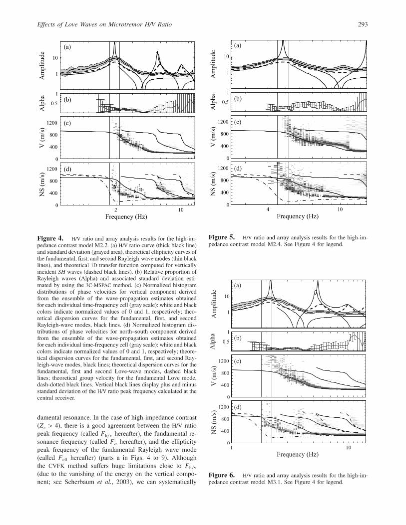
damental resonance. In the case of high-impedance contrast(Zc > 4), there is a good agreement between the H/V ratiopeak frequency (called Fh=v hereafter), the fundamental re-sonance frequency (called Fo hereafter), and the ellipticitypeak frequency of the fundamental Rayleigh wave mode(called Fell hereafter) (parts a in Figs. 4 to 9). Althoughthe CVFK method suffers huge limitations close to Fh=v

(due to the vanishing of the energy on the vertical compo-nent; see Scherbaum et al., 2003), we can systematically

1

10

Am

plitu

de(a)

0.5

1

Alp

ha (b)

0

400

800

1200

V (

m/s

)

(c)

2 100

400

800

1200

NS

(m/s

)

Frequency (Hz)

(d)

Figure 4. H/V ratio and array analysis results for the high-im-pedance contrast model M2.2. (a) H/V ratio curve (thick black line)and standard deviation (grayed area), theoretical ellipticity curves ofthe fundamental, first, and second Rayleigh-wave modes (thin blacklines), and theoretical 1D transfer function computed for verticallyincident SH waves (dashed black lines). (b) Relative proportion ofRayleigh waves (Alpha) and associated standard deviation esti-mated by using the 3C-MSPAC method. (c) Normalized histogramdistributions of phase velocities for vertical component derivedfrom the ensemble of the wave-propagation estimates obtainedfor each individual time-frequency cell (gray scale): white and blackcolors indicate normalized values of 0 and 1, respectively; theo-retical dispersion curves for the fundamental, first, and secondRayleigh-wave modes, black lines. (d) Normalized histogram dis-tributions of phase velocities for north–south component derivedfrom the ensemble of the wave-propagation estimates obtainedfor each individual time-frequency cell (gray scale): white and blackcolors indicate normalized values of 0 and 1, respectively; theore-tical dispersion curves for the fundamental, first, and second Ray-leigh-wave modes, black lines; theoretical dispersion curves for thefundamental, first and second Love-wave modes, dashed blacklines; theoretical group velocity for the fundamental Love mode,dash-dotted black lines. Vertical black lines display plus and minusstandard deviation of the H/V ratio peak frequency calculated at thecentral receiver.

1

10

Am

plitu

de

(a)

0.5

1

Alp

ha (b)

0

400

800

1200

V (

m/s

)

(c)

4 100

400

800

1200

NS

(m/s

)Frequency (Hz)

(d)

Figure 5. H/V ratio and array analysis results for the high-im-pedance contrast model M2.4. See Figure 4 for legend.

1

10

Am

plitu

de

(a)

0.5

1

Alp

ha (b)

0

400

800

1200

V (m

/s)

(c)

1 100

400

800

1200

NS

(m/s

)

Frequency (Hz)

(d)



identify the presence of the fundamental Rayleigh mode inthe vertical noise wave field from Fh=v up to the maximumcomputed frequency (parts c in Figs. 4 to 9). At higher fre-quency, we can also note the presence of higher modes,which have, however, no influence on the fundamentalH/V peak. Such higher modes may have an influence in caseof multiple H/V peaks, this is a topic out of the scope of thepresent article. Note also that phase-velocity estimates ob-tained by using the horizontal component fit the fundamentalLove mode rather well (Figs. 4d to 9d). This is explained bythe relative proportion of Rayleigh waves (α) exhibiting val-ues of about 0.2 at the H/V ratio peak frequency (Figs. 4b to9b), strongly indicating that noise synthetics are dominatedby Love waves in the horizontal plane. This might be a biasrelated to the simulation method, but such a domi-nance has also been actually observed at several sites inEurope by Köhler et al. (2006)

In case of moderate-impedance contrast (3 < Zc ≤ 4),there is a discrepancy between Fh=v and Fell, suggesting thatthe H/V ratio peak is not due to the fundamental Rayleighwave mode (Figs. 10a and 11a). Moreover, at low frequency,the phase velocity estimates do not fit the theoretical phasevelocities of the fundamental Rayleigh-wave mode, suggest-ing that the fundamental Rayleigh mode is not responsiblefor the H/V ratio peak frequency. Nevertheless, there is agood agreement between Fh=v and Fo (deviation less than20%). A second, small-amplitude H/V ratio peak can be no-

ticed for the M3.3 model at 1.8 Hz (Fig. 10a). The origin ofthis peak cannot be deduced from our array analysis; it couldbe due either to a higher Rayleigh-wave mode or an S-waveresonance within a surficial layer of the soil profile (Fig. 10c,d). Once again the presence of the fundamental Love modecan be identified from the phase velocity estimates on hor-izontal component (Figs. 10d and 11d), and the relativeproportion of Rayleigh waves (α) exhibit values between0.1–0.2 at the H/V ratio peak frequency (Figs. 10b and 11b).

In case of low-impedance contrast (Zc ≤ 3), we can dis-tinguish two different situations. In the first case, modelM2.3, there is no ellipticity peak, but the H/V curve exhibitsone peak whose frequency (Fh=v) agrees with Fo (both infrequency and amplitude) (Fig. 12a). The phase velocity es-timates could correspond to those of fundamental Rayleigh-wave mode, fundamental Love-wave mode and/or S waveswithin the bedrock (Fig. 12d). It is thus quite difficult to iden-tify clearly which waves are responsible for the H/V peak insuch a situation. However, because the H/V peak amplitudematches the theoretical amplification factor, it strongly sug-gests that the H/V ratio is due to an S-wave resonance. In thesecond case, model M4.4, the fundamental Rayleigh-wavemode exhibits an ellipticity peak but there is a large discre-pancy between Fh=v and Fell, while there is a good agreementbetween Fh=v and Fo (deviation less than 20%) (Fig. 13a).Again, at the H/V ratio peak frequency, the Rayleigh-wavephase velocity estimates do not fit the theoretical phase ve-locities of the fundamental Rayleigh-wave mode (Fig. 13c),while on the horizontal component, phase velocities agree tothe theoretical dispersion curve of fundamental Love-wavemode (Fig. 13d). The relative proportion of Rayleigh waves(α) exhibits values between 0.1 and 0.2 (Fig. 13b) at the H/Vpeak frequency.

Discussion

The two initial hypotheses on the origin of the H/V ratiopeak discussed in the beginning of the present article were(1) the S-wave resonance within the sedimentary fill (Naka-mura, 1989, 2000), and (2) the horizontal polarization of theRayleigh waves (ellipticity peak) (Lachet and Bard, 1994;Kudo, 1995; Bard, 1998; Bonnefoy-Claudet, Cornou, et. al.,2006). The in-depth investigation of noise wave-field struc-ture at the H/V peak frequency shows that the second hypoth-esis (Rayleigh wave ellipticity) is fulfilled in the case of high-impedance contrast, but is not always satisfied in the case oflow or moderate contrast. The CVFK analysis performed onhorizontal components, and the low values of the relativeproportion of Rayleigh waves α (from 0.05 to 0.2), revealthe systematic presence of fundamental Love mode in thesimulated ambient noise wave field (up to 85%).

In the case of moderate- and high-impedance contrasts,the Airy phase frequency of fundamental Love modematches the H/V ratio peak frequency as shown by frequencydependent group velocity of Love waves (Figs. 4 to 11).Because the Airy-phase frequency of Love waves corre-

1

10

Am

plitu

de(a)

0.5

1

Alp

ha (b)

0

400

800

1200

V (

m/s

)

(c)

1 100

400

800

1200

NS

(m/s

)

Frequency (Hz)

(d)



sponds to a bump of energy on both horizontal components,the H/V ratio of the Fourier amplitude spectra may thus beenhanced by this strong energy on the horizontal component.In other words, it would mean that the Airy phase of Lovewaves may even be responsible for the H/V ratio.

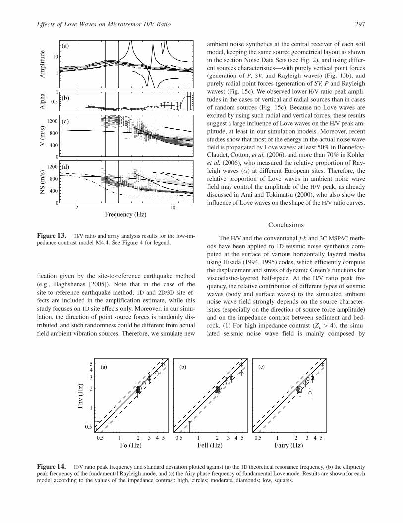
To check this hypothesis, we compare, for every soilmodel considered in this study, the frequencies of the H/Vratio peak (Fh=v) with the ones of the theoretical fundamentalresonance Fo (Fig. 14a), the fundamental Rayleigh mode el-lipticity Fell (Fig. 14b) and the Airy phase of fundamentalLove mode FAiry (Fig. 14c). The largest deviation observedbetween the H/V ratio peak frequency and the 1D theoreticalresonance frequency does not exceed 20%. The Rayleigh-wave ellipticity explains the H/V ratio peak only in caseof high-impedance contrast and only in some moderate-impedance contrast cases (Fig. 14b). In case of low-impedance contrast, the ellipticity of Rayleigh waves cannotexplain the H/V peak ratio. Figure 14c indicates that the Airyphase of the Love-wave hypothesis is fulfilled only in thecase of high or for some moderate contrasts, while it isnot satisfied in the case of a low-impedance contrast. Theseresults strongly suggest that the S-wave impedance contrast

is a key parameter controlling the origin of the H/V ratiopeak. This origin is then not unique and involves Ray-leigh-wave ellipticity, Love-wave Airy phases, and/or theS-wave resonance. Nevertheless, whatever its origin, theH/V ratio peak frequency provides a good estimation ofthe resonance frequency, at least for the 1D media shownin this study.

The estimation of the amplification using ambient noise-based method is still a challenge in the earthquake engineer-ing community. Nakamura (1989) claims that H/V peakamplitude provides a consistent estimate of the site amplifi-cation function, while others (Lachet and Bard, 1994; Kudo,1995; Bard, 1998; Fäh et al., 2001; Haghshenas, 2005; Bon-nefoy-Claudet, Cornou, et al., 2006) claim the opposite. Toevaluate the robustness of the H/V method to estimate the siteamplification factor, we compare, for each soil model, theH/V ratio peak amplitude and the theoretical site amplifica-tion (Fig. 15a). Except for the low-impedance cases, the H/Vratio peak amplitude observed from seismic noise syntheticsalways overestimates the site amplification factor. Thisobservation contradicts previous field results showing thatactual H/V ratio peaks amplitude underestimates the ampli-

1

10

Am

plitu

de

(a)

0.5

1A

lpha (b)

0

400

800

1200

V (

m/s

)

(c)

2 100

400

800

1200

NS

(m/s

)

Frequency (Hz)

(d)

Figure 8. H/V ratio and array analysis results for the high-impedance contrast model M4.1. See Figure 4 for legend.


1

10

Am

plitu

de(a)

0.5

1

Alp

ha (b)

0

400

800

1200

V (

m/s

)

(c)

2 100

400

800

1200

NS

(m/s

)

Frequency (Hz)

(d)


1

10

Am

plitu

de

(a)

0.5

1

Alp

ha (b)

0

800

1600

V (

m/s

)

(c)

1 80

800

1600

NS

(m/s

)

Frequency (Hz)

(d)

Figure 10. H/V ratio and array analysis results for the moderate-impedance contrast model M3.3. See Figure 4 for legend.

1

10

Am

plitu

de

(a)

0.5

1

Alp

ha (b)

0

400

800

1200

V (

m/s

)

(c)

2 100

400

800

1200

NS

(m/s

)Frequency (Hz)

(d)

Figure 11. H/V ratio and array analysis results for the moderate-impedance contrast model M4.3. See Figure 4 for legend.

1

10

Am

plitu

de

(a)

0.5

1

Alp

ha (b)

0

400

800

1200

V (

m/s

)

(c)

2 100

400

800

1200

NS

(m/s

)

Frequency (Hz)

(d)

Figure 12. H/V ratio and array analysis results for the low-im-pedance contrast model M2.3. See Figure 4 for legend.


fication given by the site-to-reference earthquake method(e.g., Haghshenas [2005]). Note that in the case of thesite-to-reference earthquake method, 1D and 2D/3D site ef-fects are included in the amplification estimate, while thisstudy focuses on 1D site effects only. Moreover, in our simu-lation, the direction of point source forces is randomly dis-tributed, and such randomness could be different from actualfield ambient vibration sources. Therefore, we simulate new

ambient noise synthetics at the central receiver of each soilmodel, keeping the same source geometrical layout as shownin the section Noise Data Sets (see Fig. 2), and using differ-ent sources characteristics—with purely vertical point forces(generation of P, SV, and Rayleigh waves) (Fig. 15b), andpurely radial point forces (generation of SV, P and Rayleighwaves) (Fig. 15c). We observed lower H/V ratio peak ampli-tudes in the cases of vertical and radial sources than in casesof random sources (Fig. 15c). Because no Love waves areexcited by using such radial and vertical forces, these resultssuggest a large influence of Love waves on the H/V peak am-plitude, at least in our simulation models. Moreover, recentstudies show that most of the energy in the actual noise wavefield is propagated by Love waves: at least 50% in Bonnefoy-Claudet, Cotton, et al. (2006), and more than 70% in Köhleret al. (2006), who measured the relative proportion of Ray-leigh waves (α) at different European sites. Therefore, therelative proportion of Love waves in ambient noise wavefield may control the amplitude of the H/V peak, as alreadydiscussed in Arai and Tokimatsu (2000), who also show theinfluence of Love waves on the shape of the H/V ratio curves.

Conclusions

The H/V and the conventional f-k and 3C-MSPAC meth-ods have been applied to 1D seismic noise synthetics com-puted at the surface of various horizontally layered mediausing Hisada (1994, 1995) codes, which efficiently computethe displacement and stress of dynamic Green’s functions forviscoelastic-layered half-space. At the H/V ratio peak fre-quency, the relative contribution of different types of seismicwaves (body and surface waves) to the simulated ambientnoise wave field strongly depends on the source character-istics (especially on the direction of source force amplitude)and on the impedance contrast between sediment and bed-rock. (1) For high-impedance contrast (Zc > 4), the simu-lated seismic noise wave field is mainly composed by

1

10

Am

plitu

de(a)

0.5

1

Alp

ha (b)

0

400

800

1200

V (

m/s

)

(c)

2 100

400

800

1200

NS

(m/s

)

Frequency (Hz)

(d)

Figure 13. H/V ratio and array analysis results for the low-im-pedance contrast model M4.4. See Figure 4 for legend.

0.5 1 2 3 4 5

0.5

1

2

345

Fo (Hz)

Fhv

(Hz)

(a)

0.5 1 2 3 4 5Fell (Hz)

(b)

0.5 1 2 3 4 5Fairy (Hz)

(c)

Figure 14. H/V ratio peak frequency and standard deviation plotted against (a) the 1D theoretical resonance frequency, (b) the ellipticitypeak frequency of the fundamental Rayleigh mode, and (c) the Airy phase frequency of fundamental Love mode. Results are shown for eachmodel according to the values of the impedance contrast: high, circles; moderate, diamonds; low, squares.


both fundamental Rayleigh- and Love-wave modes. (2) Formoderate-impedance contrast (3 < Zc ≤ 4), the fundamentalRayleigh-wave mode exists, but is not predominant, whilethe fundamental Love mode strongly dominates the simu-lated wave field. (3) For low-impedance contrast (Zc ≤ 3),the contribution of the fundamental Rayleigh mode to theseismic noise wave field is rather small, and the simulatedwave field is mainly composed by fundamental Love-wavemode and S waves.

Although the origin of the H/V ratio peak is not uniqueand could be explained by the Rayleigh wave ellipticity and/or the Airy phase of Love waves and/or the S-wave reso-nance, we show the robustness of the H/V peak frequencyto provide a good estimate of the 1D theoretical resonancefrequency, whatever the impedance contrast (at least forthe 1D soil structures presented here).

On the other hand, this study points out the influence ofthe direction of point source force on the H/V peak ampli-tude. When sources are vertical or radial, the simulatedH/V peak amplitude is significantly smaller than when con-sidering random sources. This clearly demonstrates a largeinfluence of the relative proportion of Love waves in the si-mulated ambient noise wave field on the H/V peak amplitude,and simultaneously indicates that the simulation methodshould be carefully worked out to include a realistic propor-tion of vertical, radial, and tangential forces to reproduce thereality. It may well be that the present assumption of randomsources with random angles is overemphasizing the role ofLove waves, but answering this question requires a muchlarger number of carefully measured sites with 3C sensorsto reliably derive the actual Rayleigh-to-Love proportion(which may also be different for long-period, natural micro-seisms and short-period, man-made microtremors). In any

case, this simulation work indicates that the H/V methodis not reliable for providing a correct estimation of thesite amplification, at least when ambient vibrations are re-lated with local surfaces sources (i.e., for microtre-mors [f > 1 Hz]).

It is worth concluding by emphasizing the possibilitiesand limitations of the H/V method for horizontally stratifiedmedia that the method always provides a good estimate ofthe resonance frequency while, in most cases (when surfacewaves dominate the ambient noise wave field), the methodfails to provide the correct amplification factor. To go aheadand prolongate this work, it is now necessary to performsimilar analysis not only on more complex media such as2D/3D structures (e.g., sedimentary basin, rough or slopinginterfaces between sediment and bedrock; see Cornou,2005; Guillier et al., 2006; Roten et al., 2006), but alsoon real ambient noise recordings (Köhler et al., 2006).

Acknowledgments

We thank the participants of the SESAME project, especially F.Cotton, for helpful discussions, comments, and suggestions. We thankM. Ohrnberger for providing the source code for array software. This workwas partly supported by the European Union research program Energy,Environment, and Sustainable Development (European Community Con-tract Number EVG1-CT-2000-00026). Most of the computations were per-formed at the Service Commum de Calcul Intensif de l’Observatoire deGrenoble, France.

References

Aki, K. (1957). Space and time spectra of stationary stochastic waves, withspecial reference to microtremors, Bull. Earthquake Res. Inst. 35, 415–457.

0 2 4 60

6

12

18

24

Ao

Ahv

(a) Random sources

0 2 4 6Ao

(b) Vertical sources

0 2 4 6Ao

(c) Radial sources

Figure 15. H/V ratio peak amplitude and standard deviation plotted against the site amplification given by the 1D theoretical transferfunction. H/V curves are calculated for different sets of noise synthetics computed with various directions of point source forces: (a) randomlygenerated in 3D space, (b) vertical, and (c) radial. Results are shown for each model according to the values of the impedance contrast: high,circles; moderate, diamonds; low, squares.


Arai, H., and K. Tokimatsu (2000). Effects of Rayleigh and Love waves onmicrotremor H/V spectra, in 12th World Conf. on Earthquake Engi-neering, Auckland, New Zealand, paper 2232.

Asten, M. (2006). Site shear velocity profile interpretation from microtremorarray data by direct fitting of SPAC curves, in 3rd Int. Symposium onthe Effects of Surface Geology on Seismic Motion, Grenoble, France,paper 99.

Atakan, K., P.-Y. Bard, F. Kind, B. Moreno, P. Roquette, and A. Tento, andthe , and SESAME-Team (2004). J-SESAME: a standardized softwaresolution for the H/V spectral ration technique, in Proc. of the 13thWorld Conf. on Earthquake Engineering, paper 2270, Vancouver,Canada, August 2004.

Bard, P.-Y. (1998). Microtremor measurements: a tool for site effect estima-tion?, in 2nd Int. Symp. on the Effects of Surface Geology on SeismicMotion, Yokohama, Japan, 3, 1251–1279.

Bard, P.-Y., and the , and SESAME-Team (2005). Report D23.12, Guide-lines for the implementation of the H/V spectral ratio technique onambient vibrations measurements, processing and interpretation inEuropean Commission: Research General Directorate, Project No.EVG1-CT-2000-00026, SESAME, 62 pp.: available online at http://sesame‑fp5.obs.ujf‑grenoble.fr (last accessed January 2008).

Bettig, B., P. Y. Bard, F. Scherbaum, J. Riepl, F. Cotton, C. Cornou, and D.Hatzfeld (2001). Analysis of dense array noise measurements using themodified spatial auto-correlation method (SPAC): application to theGrenoble area, Boll. Geof. Teorica Appl. 42, nos. 3–4, 281–304.

Bonnefoy-Claudet, S. (2004). Nature du bruit de fond sismique: implicationspour les études des effets de site, Ph.D. Thesis, University JosephFourier, Grenoble, France, 241 pp. (in French with English abstract).

Bonnefoy-Claudet, S., C. Cornou, P.-Y. Bard, F. Cotton, P. Moczo, J. Kris-tek, and D. Fäh (2006). H/V ratio: a tool for site effects evaluation:results from 1D noise simulations, Geophys. J. 167, no. 2, 827–837.

Bonnefoy-Claudet, S., C. Cornou, J. Kristek, M. Ohrnberger, M. Wathelet,P.-Y. Bard, P. Moczo, D. Fäh, and F. Cotton (2004). Simulation of seis-mic ambient noise: I. results of H/Vand array techniques on canonicalmodels, in 13th World Conf. on Earthquake Engineering, Vancouver,Canada, paper 1120.

Bonnefoy-Claudet, S., F. Cotton, and P.-Y. Bard (2006). The nature of theseismic noise wave field and its implication for site effects studies: aliterature review, Earth Sci. Rev. 79, nos. 3–4, 205–227.

Cornou, C. (2005). Reports D11.10 and D17.10, Set of noise synthetics forH/Vand array studies from simulation of real sites and comparison fortest sites in European Commission: Research General Directorate, Pro-ject No. EVG1-CT-2000-00026, SESAME, 62 pp.: available online athttp://sesame‑fp5.obs.ujf‑grenoble.fr (last accessed January 2008).

Di Giulio, G., A. Rovelli, F. Cara, R. M. Azzara, F. Marra, R. Basili, and A.Caserta (2003). Long-duration asynchronous ground motions in theColfiorito plain, central Italy, observed on a two-dimensional densearray, J. Geophys. Res. 108, 2486–2500.

Fäh, D. (1997). Microzonation of the city of Basel, J. Seism. 1, no. 1, 87–102.

Fäh, D., F. Kind, and D. Giardini (2001). A theoretical investigation of aver-age H/V ratios, Geophys. J. 145, no. 2, 535–549.

Field, E., and K. Jacob (1993). The theoretical response of sedimentarylayers to ambient seismic noise, Geophys. Res. Lett. 20, no. 24,2925–2928.

Fukushima, Y., S. Kinoshita, and H. Satho (1992). Measurement of Q forS-wave in mudstone at Chikura, Japan: comparison of incident andreflected phases in boreholes seismograms, Bull. Seismol. Soc. Am.82, 148–163.

Gitterman, Y., Y. Zaslavsky, A. Shapira, and V. Shtivelman (1996). Empiri-cal site response evaluations: case studies in Israel, Soil Dyn. Earth-quake Eng. 15, no. 7, 447–463.

Guillier, B., C. Cornou, J. Kristek, S. Bonnefoy-Claudet, P.-Y. Bard, D. Fäh,and P. Moczo (2006). Simulation of seismic ambient vibrations: doesthe H/V provide quantitative information on 2D–3D structure, in 3rdInt. Symposium on the Effects of Surface Geology on Seismic Motion,Grenoble, France, paper 153.

Haghshenas, E. (2005). Conditions géotechniques et aléa sismique local àTéhéran, Ph.D. Thesis, University Joseph Fourier, Grenoble, France,288 pp. (in French with English abstract).

Hauksson, K., T. Teng, and T. L. Henyey (1987). Results from a 1500 mdeep, three-level downhole seismometer array: site response, low Qvalue, and fmax, Bull. Seismol. Soc. Am. 77, 1883–1904.

Hisada, Y. (1994). An efficient method for computing Green’s functions fora layered half-space with sources and receivers at close depths, Bull.Seismol. Soc. Am. 84, no. 5, 1456–1472.

Hisada, Y. (1995). An efficient method for computing Green’s functions fora layered half-space with sources and receivers at close depths (part 2),Bull. Seismol. Soc. Am. 85, no. 4, 1080–1093.

Jongmans, D., K. Pitilakis, D. Demanet, D. Raptakis, J. Riepl, C. Horrent, G.Tsokas, K. Lontzetidis, and P.-Y. Bard (1998). EURO-SEISTEST:determination of the geological structure of the Volvi basin and vali-dation of the basin response, Bull. Seismol. Soc. Am. 88, no. 2, 473–487.

Köhler, A., M. Ohrnberger, and F. Scherbaum (2006). The relative fractionof Rayleigh and Love waves in ambient vibration wave fields at dif-ferent European sites, in 3rd Int. Symposium on the Effects of SurfaceGeology on Seismic Motion, Grenoble, France, paper 83.

Köhler, A., M. Ohrnberger, F. Scherbaum, M. Wathelet, and C. Cornou(2007). Assessing the reliability of the modified three-componentspatial autocorrelation technique, Geophys. J. Int. 168, no. 2,779–796.

Konno, K., and T. Ohmachi (1998). Ground-motion characteristics estimatedfrom spectral ratio between horizontal and vertical components ofmicrotremor, Bull. Seismol. Soc. Am. 88, no. 1, 228–241.

Kudo, K. (1995). Practical estimates of site response: state-of-art report, in5th Int. Conf. on Seismic Zonation, Nice, France.

Kvaerna, T., and F. Ringdahl (1986). NORSAR Scientific Report 1-86/87,Stability of various f-k estimation techniques, in Semiannu. Tech.Summ., 1 October 1985–31 March 1986, Kjeller, Norway, 29–40.

Lachet, C., and P.-Y. Bard (1994). Numerical and theoretical investigationson the possibilities and limitations of Nakamura’s technique, J. Phys.Earth 42, no. 4, 377–397.

Lermo, J., and F. J. Chavez-Garcia (1993). Site effects evaluation using spec-tral ratios with only one station, Bull. Seismol. Soc. Am. 83, no. 5,1574–1594.

Lermo, J., and F. J. Chavez-Garcia (1994). Are microtremors useful in siteresponse evaluation?, Bull. Seismol. Soc. Am. 84, no. 5, 1350–1364.

McMamara, D., and R. Buland (2004). Ambient noise levels in thecontinental United States, Bull. Seismol. Soc. Am. 94, no. 4, 1517–1527.

Moczo, P., and J. Kristek (2002). Report D02.09, FD code to generate noisesynthetics, in European Commission: Research General Directorate,Project No. EVG1-CT-2000-00026, SESAME, 31 pp.: available onlineat http://sesame‑fp5.obs.ujf‑grenoble.fr (last accessed January 2008).

Nakamura, Y. (1989). A method for dynamic characteristics estimation ofsubsurface using microtremor on the ground surface, Q. Rept. Railw.Tech. Res. Inst. 30, no. 1, 25–30.

Nakamura, Y. (1996). Real-time information systems for hazards mitigation,in 11th World Conf. on Earthquake Engineering, Acapulco, Mexico.

Nakamura, Y. (2000). Clear identification of fundamental idea of Naka-mura’s technique and its applications, in 12th World Conf. on Earth-quake Engineering, Auckland, New Zealand.

Nogoshi, M., and T. Igarashi (1971). On the amplitude characteristics ofmicrotremor (part 2), J. Seismol. Soc. Japan 24, 26–40 (in Japanesewith English abstract).

Ohrnberger, M. (2004). Report D18.06, User manual for software packageCAP: a continuous array processing toolkit for ambient vibration arrayanalysis, in European Commission: Research General Directorate, Pro-ject No. EVG1-CT-2000-00026, SESAME, 83 pp.: available online athttp://sesame‑fp5.obs.ujf‑grenoble.fr (last accessed January 2008).

Ohrnberger, M., E. Schissele, C. Cornou, S. Bonnefoy-Claudet, M. Wathe-let, A. Savvaidis, F. Scherbaum, and D. Jongmans (2004). Frequencywavenumber and spatial autocorrelation methods for dispersion curve


determination from ambient vibration recordings, in 13th World Conf.on Earthquake Engineering, Vancouver, Canada, paper 946.

Ohrnberger, M., E. Schissele, C. Cornou, M. Wathelet, A. Savvaidis, F.Scherbaum, D. Jongmans, and F. Kind (2004). Microtremor arraymeasurements for site effect investigations: comparison of analysismethods for field data crosschecked by simulated wave fields, in13th World Conf. on Earthquake Engineering, Vancouver, Canada,paper 940.

Okada, H. (2003). The microtremor survey, in Society of Exploration Geo-physicists, American Geophysical Monograph, 13, 135 pp.

Roten, D., D. Fäh, C. Cornou, and D. Giardini (2006). Two-dimensionalresonances in Alpine valleys identified from ambient vibration wavefields, Geophys. J. Int. 165, no. 3, 889–905.

Scherbaum, F., K.-G. Hinzen, and M. Ohrnberger (2003). Determination ofshallow shear wave velocity profiles in the Cologne, Germany areausing ambient vibrations, Geophys. J. Int. 152, no. 3, 597–612.

Seekins, L. C., L. Wennerberg, L. Marghereti, and H.-P. Liu (1996). Siteamplification at five locations in San Francisco, California: A compari-son of S waves, codas, and microtremors, Bull. Seismol. Soc. Am. 86,no. 3, 627–635.

Tokeshi, J. C., and Y. Sugimura (1998). On the estimation of the naturalperiod of the ground using simulated microtremors, in 2nd Int. Symp.on the Effects of Surface Geology on Seismic Motion, Yokohama,Japan, 2, 651–664.

Wakamatsu, K., and Y. Yasui (1996). Possibility of estimation for amplifica-tion characteristics of soil deposits based on ratio of horizontal to ver-tical spectra of microtremors, in 11th World Conf. on EarthquakeEngineering, Acapulco, Mexico.

Wang, Z., R. Street, and E. Woolery (1994). Qs estimation for unconsoli-dated sediments using first-arrival SH critical refractions, J. Geophys.Res. 99, no. B7, 13,543–13,552.

Institut de Radioprotection et de Sureté NucléaireBP 1792262 Fontenay-aux-Roses, Cedex, France

(S.B.)

Institute of GeosciencesPotsdam UniversityKarl-Liebknecht-Str. 24Haus 2714476 Potsdam, Germany

(A.K.)

Laboratoire de Géophysique Interne et de Tectonophysique, Institut deRecherche et de Développement, Laboratoire Central desPonts-et-ChausséesMaison des GéosciencesJoseph Fourier UniversityBP 5338041 Grenoble Cedex 9, France

(C.C., M.W., P.-Y.B.)

Manuscript received 14 March 2007


Effects of Love Waves on Microtremer HV Ratio

Documents

Transcript of Effects of Love Waves on Microtremer HV Ratio