Effects of Homeownership on Children: The Role of ...€¦ · Neighborhood Characteristics and...

FRBNY Economic Policy Review / June 2003 87

Effects of Homeownership on Children: The Role of Neighborhood Characteristics and Family Income

1. Introduction

recent press release from the U.S. Department of Housingand Urban Development (HUD) captures the wide-

ranging benefits increasingly being attributed to homeownership: “Homeowners accumulate wealth as the investment in their homes grows, enjoy better living conditions, are often more involved in their communities, and have children who tend on average to do better in school and are less likely to become involved with crime. Communities benefit from real estate taxes homeowners pay, and from stable neighborhoods homeowners create” (U.S. Department of Housing and Urban Development 2000). This credo undergirds the last decade’s push to extend homeownership to all Americans, particularly low-income families and racial minorities. Because it is believed to strengthen not only families but communities, homeownership is being promoted as an important strategy for regenerating distressed urban neighborhoods.

Enormous amounts of money, both public and private, are being invested in increasing the homeownership rate. From the $2 trillion “American Dream Commitment” of Fannie Mae, to the multimillion-dollar homeownership programs of the Enterprise Foundation, the Local Initiatives Support Corporation, and the Neighborhood Reinvestment

Corporation, to the millions of dollars of programs and incentives under HUD’s control, a consistent view of homeownership as a “silver bullet” has emerged. Incentives for homeownership even appear in the welfare reform plans of a number of states.

Despite this significant investment, there is remarkably little known about the real effects of homeownership on either homeowners, their children, or their communities. This paper focuses on one aspect of homeownership: its potential long-term effects on children. Several recent studies have found that growing up in a homeowning family exerts positive effects on children’s development and outcomes (Green and White 1997; Aaronson 2000; Boehm and Schlottman 1999; Haurin, Parcel, and Haurin 2000). But what accounts for these positive effects, and whether other features may either strengthen or weaken them, is unclear. One such feature is the neighborhood. Since many families who will become new homeowners under current policies promoting homeownership for the poor will purchase homes in areas traditionally thought of as troubled or distressed, it is important to understand whether neighbor-hood characteristics play a role in the effects of homeownership on children’s outcomes.

To our knowledge, only Aaronson (2000) has explored this link. He finds that parental homeownership in low-income census tracts has a more positive effect on high-school

Joseph M. Harkness and Sandra J. Newman

Joseph M. Harkness is a research statistician at the Institute for Policy Studies at Johns Hopkins University; Sandra J. Newman is a professor of policy studies and the director of the Institute for Policy Studies.

The authors gratefully acknowledge the Fannie Mae Foundation for its support of this research; the helpful insights of their discussant, Frank Braconi; and Sally Katz, Amy Robie, and Laura Vernon-Russell for research assistance and production help. Certain copyrighted material is used with the permission of the Fannie Mae Foundation. The views expressed are those of the authors and do not necessarily reflect the position of the Federal Reserve Bank of New York or the Federal Reserve System.

A

88 Effects of Homeownership on Children

graduation than it does in high-income census tracts. This intriguing result suggests that homeownership may buffer children against the damaging effects of growing up in distressed neighborhoods. But Aaronson also finds that neighborhood residential stability enhances the positive effects of homeownership on high-school graduation, which suggests that at least some of the positive effects of homeownership found in other studies may be attributed to the greater resi-dential stability of the neighborhoods where homeowners live.

Very different policy recommendations emerge from these two results. According to the first, homeownership should be promoted even—or especially—in very low-income neighborhoods. According to the second, neighborhoods that are residentially stable are preferred, and efforts to stabilize distressed neighborhoods by encouraging low-income families to purchase homes there may carry significant risks for the “pioneers,” the first homeowners in a distressed area.

Another neighborhood feature that may play a role is the homeownership rate, which has largely been ignored in the sizable and growing body of research on the effects of distressed neighborhoods on the life chances of children (see reviews by Jencks and Mayer [1990], Haveman and Wolfe [1995], Gephart [1997], Ellen and Turner [1998], and Moffitt [2001]).1 But if the silver-bullet view of homeownership benefiting not only the immediate homeowning family but also the surrounding community is correct, then the positive effects of homeownership on children’s outcomes may be attributed to the tendency for homeowning families to live in neighbor-hoods of homeowners—not to the family’s homeownership status, per se.

This scenario also raises important policy concerns. As with neighborhood residential stability, if the homeownership rate in a neighborhood is responsible for the improved outcomes of children who live there, then policies encouraging poor families to purchase homes in areas where there are few homeowners may be good for the neighborhood but bad for the individual family. Since moving a neighborhood from a low to a high rate of homeownership is likely to be a long-term process, the early “pioneer” homeowners would derive few or no benefits and, in fact, may bear considerable costs such as low property values, high crime rates, poor schools, and, perhaps most importantly, the inability to move elsewhere easily (that is, selling a home is much more difficult than breaking a lease).

A second feature that may alter the effects of homeownership on children is family income. Interest in this topic is also motivated by policy concerns, since most homeownership promotion policies target low-income families. Previous research has examined this question only indirectly, and results are conflicting. For example, Green and White (1997) report estimates from one data set showing that

family income matters more for children of renters than for children of homeowners. They interpret this to mean that the positive effects of homeownership on children erode with higher incomes. But using another data set, Green and White find that ownership of a more expensive home is more beneficial to children, consistent with Aaronson’s (2000) finding that greater home equity is associated with better outcomes. Since higher income families tend to both live in more expensive housing and have more equity in their homes, these results suggest that homeownership primarily benefits children of higher income families.

This exploratory paper first tests whether homeownership has equally positive effects for children of low-income and higher income families. Focusing on the low-income group, it then examines whether, and how, these homeownership effects are influenced by neighborhood attributes. The next section reviews theories of the ways in which homeownership could benefit children and how these benefits could be modified by neighborhood characteristics. We then describe our data, methods, and results. A discussion of the findings and their policy implications follows.

2. Background

There are three broad sets of explanations for the effects of homeownership on children’s outcomes. According to the first, there is a direct link between family homeownership and children’s outcomes. The second set, in contrast, posits that differences in neighborhoods, not family homeownership, explain why children of homeowners have better outcomes. The third set speculates that neither homeownership nor neighborhoods by themselves are the key explanatory factors, but rather that homeownership is associated with more favorable outcomes only under certain neighborhood characteristics. We refer to these as direct, indirect, and interactive homeownership effects, respectively.

2.1 Direct Homeownership Effects

The literature suggests four paths through which parental homeownership could affect children’s outcomes: 1) parenting practices, 2) physical environment, 3) residential mobility, and 4) wealth.

Haurin, Parcel, and Haurin (2000) find that homeowning parents provide a more stimulating and emotionally supportive environment for their children, which significantly


improves cognitive ability and reduces behavioral problems. They attribute the improved parenting of homeowners to either their greater investment in their properties or residential stability, both of which are explored below. Another explanation, supported by some empirical evidence, is that homeownership produces greater life satisfaction or self-esteem for adults, which, in turn, provides a more positive home environment for children (Balfour and Smith 1996; Rossi and Weber 1996; Rohe and Basolo 1997; Rohe and Stegman 1994b). Sherraden (1991) argues that the psychological benefits of homeownership for adults derive from its function as an asset. Green and White (1997) offer several wide-ranging hypotheses of the potential links between homeownership and children’s outcomes, including the possibility that experience with contractors and repair personnel may improve homeowning parents’ interpersonal and management skills, which may transfer to their children.

Except for gross, health-threatening inadequacies, little is known about how children are affected by their dwellings’ conditions.2 But it is plausible that the physical features of owned versus rental housing may also affect children’s development. More than four-fifths of owned homes are single-family, detached structures, compared with less than one-fourth of rental properties.3 These environments may be better for children because, for example, they are likely to be more spacious and private. Owned homes are also likely to be in better physical condition because owner occupants are more likely to invest in the quality of their dwellings (Galster 1987; Mayer 1981; Spivack 1991). Since higher quality housing is generally more expensive, the previously cited findings of Green and White (1997) and Aaronson (2000)—that more expensive housing has favorable long-term effects on children—lend support to the view that the physical quality of housing matters. But their findings also suggest that the lower quality housing affordable to low-income homebuyers may not benefit their children significantly.

Several studies demonstrate that moving can harm children’s educational outcomes (Haveman, Wolfe, and Spaulding 1991; Astone and McLanahan 1994; Jordan et al. 1996; Hanushek, Kain, and Rivkin 1999), and there is substantial evidence that homeowners move far less often than renters (Barrett, Oropes, and Kanan 1994; Hanushek and Quigley 1978; Newman and Duncan 1979; Quigley and Weinberg 1977). Included here are recent studies that detect a causal, not merely correlational, impact of homeownership on a reduced likelihood of moving (Ioannides and Kan 1996; Kan 2000). Aaronson (2000) investigates this issue, and finds that much of the positive effect of homeownership on childhood outcomes can be attributed to its impact on residential stability.

Home equity is the most significant asset held by most American families, and for many, their only asset. One function of assets is that they can be leveraged during times of need, which could benefit children. For example, homeowning parents can borrow money against the equity in their home to finance a child’s college education. In addition, inheritable wealth constitutes a child’s claim on the future, enabling long-term planning and higher expectations (Conley 1999). Empirical evidence suggests a link between home value or equity and favorable youth outcomes (Aaronson 2000; Boehm and Schlottman 1999; Conley 1999), such as the likelihood of acquiring a college education. However, these estimates could be biased upward because they are likely to be picking up at least some of the impact of neighborhood characteristics, which are not controlled for in these studies. In addition, homeownership as an asset-building tool could fail to benefit poor children if the down payment and ongoing maintenance costs absorb resources that might otherwise be invested in children’s development. The tax advantages of homeownership are also disproportionately reaped by the more affluent, which could lead to better outcomes for their children.

2.2 Indirect Homeownership Effects

A second perspective is that the findings of previous studies on the benefits of homeownership are spurious because it is the better neighborhoods and schools experienced by children of homeowners—not growing up in an owned home—that account for their better outcomes.4 Because homeowners generally live in communities characterized by higher incomes, higher rates of homeownership, and greater residential stability, their children will benefit from these positive neighborhood externalities.

Homeownership may generate positive neighborhood externalities through its effect on either physical or social capital. As noted, owner-occupied houses appear to be better maintained than rental properties (Galster 1987; Mayer 1981; Spivack 1991), providing one form of neighborhood amenity that may benefit children. But theory also suggests that because homeowners’ financial stake in their properties is illiquid and not easily extracted, homeowners will be more active in maintaining or improving the quality of their neighborhoods, not just their own houses.

A substantial body of research suggests that homeowners are more attached to their communities and more active in community affairs (Rossi and Weber 1996; DiPasquale and Glaeser 1999; Blum and Kingston 1984; Austin and Baba 1990).


Greater community involvement could plausibly lead to greater community social capital. Sampson et al. (1997) provide strong evidence to support this link. These researchers show that homeownership, in conjunction with residential stability, generates social capital in the form of “collective efficacy,” which may produce better outcomes for children.

However, residential stability has also been shown to be an important determinant of community involvement (Kasarda and Janowitz 1974; Sampson 1988). A question raised by this body of evidence is whether homeownership itself—or the residential stability it is correlated with—is more responsible for the positive effects of homeownership on community participation. DiPasquale and Glaeser (1999) explore this issue, and find that length of residence is more important than homeownership across several key measures of community involvement. Because residentially stable neighborhoods of renters may be as beneficial to children as neighborhoods of homeowners, it is critical to distinguish analytically between a neighborhood’s homeownership rate and its residential stability.

2.3 Interactive Homeownership Effects

Finally, a third view is that the effects of homeownership on children’s outcomes vary depending on the type of neighborhood. Homeownership could buffer the effects of a distressed neighborhood if, for example, homeowning parents more aggressively monitor their children’s activities, have higher expectations for their children, or have more social capital to draw on. But the child-rearing practices of homeowners living in more prosperous neighborhoods may differ little from those of neighboring renters. This buffering hypothesis is consistent with Aaronson’s (2000) finding that growing up in a homeowning family in a low-income neighborhood has a stronger positive effect on the probability of graduating from high school than homeownership in a high-income neighborhood.

Alternatively, children of homeowners might be more, not less, affected by the conditions in their neighborhoods than renter children because of homeowners’ relatively greater residential stability. Greater residential stability reduces or eliminates the need to change schools and increases the opportunity to develop closer ties to neighbors. As a result, the characteristics of their neighborhoods—both good and bad—could exert a particularly strong influence.5 Aaronson’s (2000) finding that homeownership has more positive effects on high-school graduation in residentially stable neighborhoods is consistent with this speculation.

3. Data and Methods

This study extends and refines previous work on the effects of homeownership on children’s outcomes in several ways. Earlier investigations have focused on educational attainment effects (Green and White 1997; Aaronson 2000; Boehm and Schlottman 1999).6 We extend the set of outcomes to include teen unwed births, idleness, wage rates, and welfare receipt. Examining multiple outcomes is important because the effects of homeownership may vary by outcome. Children of homeowners may attend higher quality schools than children of renters, for example, so that identical educational attainment by the two groups may not translate into identical earnings or welfare receipt.

Second, the analysis compares results for low-income and higher income families, with “low-income” defined as having parental earnings below 150 percent of the federal poverty line.7 Although all previous studies on the effects of homeownership have controlled for income, none has explicitly tested for different effects of homeownership between low-income and higher income groups. An analytical focus on low-income families is appropriate because they are the primary target of homeownership promotion policies, and pooling low-income with higher income families could produce misleading results.8

The third way in which this paper differs from previous work is that we examine the effects of neighborhood characteristics both as independent factors and as factors that may change the way homeownership influences outcomes. Since homeowners and renters may live in very different kinds of neighborhoods, and children’s outcomes may be affected by these different neighborhoods, the failure to control for them could produce estimates that mistakenly attribute neighborhood effects to homeownership.9

We test for the simultaneous effects of three measures of neighborhood characteristics: the poverty rate, the homeownership rate, and residential stability. We include the poverty rate because we are interested in the effects of homeownership in distressed neighborhoods on children’s outcomes, and the poverty rate is a widely used indicator of neighborhood distress. The neighborhood poverty rate is also almost perfectly correlated (negatively) with neighborhood median income, which ensures comparability with the results of Aaronson (2000). We include the homeownership rate to distinguish between the effects of homeownership by a child’s parents from the homeownership level of the neighborhood. Finally, we control for neighborhood residential stability because a neighborhood’s homeownership rate is plausibly linked to residential stability (Rohe and Stewart 1996), and we


want to determine whether it is neighborhood homeownership or neighborhood stability that is responsible for neighborhood effects on children’s outcomes.

3.1 Sample

The analysis uses data from the 1968-93 waves of the geocoded Panel Study of Income Dynamics (PSID). Begun in 1968, the PSID is an ongoing longitudinal survey of U.S. households conducted by the Survey Research Center at the University of Michigan. All original household members have been followed over time. Recent research confirms that despite considerable attrition, the PSID remains representative of the population (Fitzgerald, Gottschalk, and Moffitt 1998a, 1998b; Zabel 1998).

The analysis is performed on a sample of individuals with PSID family data available each year between ages eleven and fifteen, born between 1957 and 1973. Results are first compared for two samples: 1) a low-income sample of children from families with parental earnings below 150 percent of the federal poverty threshold for at least three of the five years between ages eleven and fifteen and 2) a higher income sample comprised of the children not in the low-income sample.10 We then shift the analysis to focus exclusively on the low-income group and further restrict the sample to children whose parents were either always homeowners or always renters when the child was between ages eleven and fifteen. This latter restriction, which eliminates about 20 percent of cases, enables us to derive meaningful coefficients on the effects of homeownership while testing interactions between tenure status and neighborhood characteristics (see Appendix A for further discussion of the methodology).

3.2 Approach

We examine the effects of living in an owned home as a child on seven outcomes: 1) giving birth as an unmarried teenager (women only), 2) idleness (not working, attending school, or caring for children) at age twenty, 3) years of education at age twenty, 4) high-school completion at age twenty, 5) acquisition of post-secondary education at age twenty, 6) average hourly wage rates between ages twenty-four and twenty-eight, and 7) receipt of welfare—Aid to Families with Dependent Children (AFDC), food stamps, or other cash assistance—between ages twenty-four and twenty-eight.11

We estimate three sets of models, corresponding to the three broad conceptualizations of homeownership effects outlined earlier. The first set of models tests for the direct effects of homeownership on children’s outcomes without controls for neighborhood features. Estimates are obtained separately and compared for low-income and higher income groups. Next, we test for indirect effects by adding controls for average neighborhood characteristics experienced between ages eleven and fifteen using the low-income sample. If neighborhood differences between homeowners and renters account for a substantial portion of the beneficial effects of homeownership, the homeownership effect estimates produced by these models should be much smaller than those produced by the direct effect models. The third set of models tests for the interaction of tenure status and neighborhood characteristics by specifying interaction terms between tenure status and each of the three neighborhood characteristics (stability, homeownership rate, and poverty rate), also performed on the low-income sample only.

The analysis uses ordinary least squares to estimate the effect of homeownership on years of education and wage rates. The models for the effects of homeownership on high-school completion, acquisition of post-secondary education, idleness, and welfare receipt, which are binary (that is, whether high school was completed or not), use probit.12

A major difficulty in identifying the effects of homeowner-ship and neighborhoods on children is that they may be associated with parental characteristics that are not measured in the data and, therefore, cannot be controlled for in statistical models. The standard technique for dealing with such unmeasured variable problems is to use “instruments,” variables that are correlated with the key analytical variables (homeownership and neighborhood characteristics, in this paper) but are independent of the unmeasured characteristics. However, while finding plausible instruments for homeowner-ship is possible and has been done in other studies (Green and White 1997; Haurin, Parcel, and Haurin 2000; Aaronson 2000; Harkness and Newman 2002), it is difficult to identify credible instruments for the three neighborhood indicators tested here (Duncan, Connell, and Klebanov 1997; Duncan and Raudenbusch 1998; Moffitt 1999). Because this paper focuses on homeownership and neighborhoods, results based on instrumenting for homeownership alone would not be interpretable. In discussing the results, however, we argue that conclusions would be unlikely to change if controls for unmeasured family characteristics were added.


3.3 Policy Variables

The measure of homeownership is whether a child always lived in an owned home between ages eleven and fifteen. Three neighborhood features are included: the poverty rate, the percentage of families owning their home, and residential stability, the last being measured as the percentage of families living in the same housing unit for five or more years.13 Interactive effects between housing tenure and neighborhood are obtained by multiplying the homeownership variable by each of the neighborhood variables. In the interaction model, the neighborhood variables are specified in mean-deviation form.14 This implies that the coefficient on homeownership in these models can be readily interpreted as the effect of homeownership in the average sample neighborhood.

3.4 Control Variables

All models control for the following characteristics: 1) race, 2) gender, 3) year born, 4) age of mother when born, 5) educational attainment of household head, 6) number of children in family, 7) years in a two-parent family, 8) average annual earnings, 9) whether there is any, and the amount of, parental income (not including public assistance) in excess of earnings (average annual), 10) number of years the family relied on AFDC, food stamps, or other cash assistance (excluding Supplemental Security Income), 11) years in a city of 500,000 or more, 12) years in a city of 100,000 to 500,000, and 13) the child’s primary state of residence.15

For educational outcomes, about 25 percent of cases are missing data on grades completed at age twenty, but have data on grades completed at some other age. In these cases, we substituted educational attainment in the closest year after age twenty, if available, and in the closest year before age twenty otherwise. Because educational attainment is affected by age, the models also include a control variable for the age to which the educational attainment measure applies. Monetary values are expressed in 1997 dollars using the CPI-U, the consumer price index for all urban consumers. City sizes come from the PSID census geocode.16

Each of these variables is plausibly related to one or more outcomes examined here, and most have been used extensively in other research on determinants of children’s outcomes. The exceptions are controls for wealth other than home equity, and city size. Based on Conley’s (1999) finding that parental wealth has significant effects on children’s outcomes, we control for wealth by including a measure of income that is neither earned

nor obtained through public assistance.17 We control for city size because Page and Solon (1999) have demonstrated “the importance of being urban” on adult earnings. State dummy variables are included to account for the fact that unmeasured features of states, such as quality of education or labor market conditions, may affect outcomes (Moffitt 1994).

Although children’s outcomes may be affected by a family’s home equity and residential mobility, as described earlier, we did not include controls for these factors in the initial models because both are also likely to be affected by whether a family owns its home, as well as neighborhood characteristics. Consequently, the estimates for the effects of homeownership and neighborhoods will include the effects that operate through home equity and residential moves, and they should be interpreted accordingly. After reviewing the main results, we conduct a supplementary analysis using these excluded variables.

4. Sample Characteristics

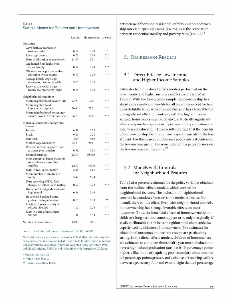
Table 1 shows the mean differences in outcomes, neighbor-hood characteristics, and family background characteristics between children of homeowners and those of renters. The differences are stark. Relative to homeowner children, renter children are 40 percent more likely to give birth as an unmarried teenager, and they are nearly twice as likely to be idle at age twenty and to rely on welfare as an adult. Their high-school graduation rate is 19 percent lower than that of homeowner children, they are only half as likely to acquire some post-secondary education, and their average hourly wage is a dollar less. These differences are all statistically significant.

Differences in the family backgrounds of renter and owner children are also dramatic. The parental income of renter children is half that of owner children, and renter children are twice as likely to grow up in a single-parent household or be on welfare. They experience an average neighborhood poverty rate of 24 percent, compared with 18 percent for owner children, and a substantially lower neighborhood homeownership rate (56 percent versus 72 percent, respectively). Surprisingly, there is little difference in the residential stability of the neighbor-hoods of these two groups. In renter neighborhoods, 57 percent of families had lived in the same residence for five years or more, compared with 58 percent in homeowner neighborhoods. The neighborhood poverty and home-ownership rates experienced by the sample children are somewhat negatively correlated (r =- .45), but the correlation


between neighborhood residential stability and homeowner-ship rates is surprisingly weak (r = .25), as is the correlation between residential stability and poverty rates (r = .11).18

5. Regression Results

5.1 Direct Effects: Low-Income and Higher Income Samples

Estimates from the direct effects models performed on the low-income and higher income samples are presented in Table 2. With the low-income sample, homeownership has statistically significant benefits for all outcomes except for teen unwed childbearing, where homeownership has a favorable but not significant effect. In contrast, with the higher income sample, homeownership has positive, statistically significant effects only on the acquisition of post-secondary education and total years of education. These results indicate that the benefits of homeownership for children are reaped primarily by the less affluent. For this reason, and because policy interest centers on the low-income group, the remainder of this paper focuses on the low-income sample alone.19

5.2 Models with Controls for Neighborhood Features

Table 2 also presents estimates for the policy variables obtained from the indirect effects models, which control for neighborhood features. The inclusion of neighborhood controls has modest effects on some model estimates, but overall, there is little effect. Even with neighborhood controls, homeownership has strong, favorable effects on most outcomes. Thus, the beneficial effects of homeownership on children’s long-term outcomes appear to be only marginally, if at all, attributable to the better neighborhood characteristics experienced by children of homeowners. The estimates for educational outcomes and welfare receipt are particularly strong. In the direct effects models, children of homeowners are estimated to complete almost half a year more of education, have a high-school graduation rate that is 13 percentage points higher, a likelihood of acquiring post-secondary education that is 6 percentage points greater, and a chance of receiving welfare between ages twenty-four and twenty-eight that is 9 percentage

Table 1

Sample Means for Renters and Homeowners

Renters Homeowners p-value

Outcomes

Gave birth as unwed teen (women only) 0.14 0.10 *

Idle at age twenty 0.25 0.14 ***

Years of education at age twenty 11.30 12.0 ***

Graduated from high school by age twenty 0.57 0.70 ***

Obtained some post-secondary education by age twenty 0.12 0.23 ***

Average hourly wage, ages twenty-four to twenty-eight 9.16 10.35

Received any welfare, ages twenty-four to twenty-eight 0.34 0.18 ***

Neighborhood conditions

Mean neighborhood poverty rate 23.9 17.9 ***

Mean neighborhood homeownership rate 56.0 72.2 ***

Mean neighborhood percentage did not move in five or more years 56.7 58.0 ***

Individual and family background features

Female 0.52 0.52

Black 0.44 0.21 ***

Year born 1966 1966 *

Mother’s age when born 25.2 26.8 ***

Whether income is greater than earnings plus transfers 0.55 0.81 ***

Parental earnings 11,080 20,920 ***

Mean amount of family income is greater than earnings plus transfers 2,380 8,070 ***

Years in two-parent family 2.25 3.65 ***

Mean number of children in family 3.64 3.45

Years receiving AFDC, food stamps, or “other” cash welfare 0.62 0.22 ***

Household head graduated from high school 0.36 0.49

Household head had some post-secondary education 0.18 0.30 **

Fraction of years in a city of 100,000-500,000 1.12 0.73 ***

Years in a city of more than 500,000 1.31 0.53 ***

Number of observations 1,495 1,081

Source: Panel Study of Income Dynamics (PSID), 1968-93.

Notes: Monetary figures are expressed in 1997 dollars. Statistical signifi-cance indicators refer to one-tailed t-test results for differences in means, unequal variances assumed. Values are weighted using age fifteen PSID individual weights. AFDC is Aid to Families with Dependent Children.

* Value is less than .05.

** Value is less than .01.

*** Value is less than .0001.


points lower. All of these estimates are highly statistically significant (p = .01), and they decline only slightly, if at all, when controls for neighborhood features are added.

The estimated effects of homeownership on children’s subsequent idleness and wage rates are also favorable, but somewhat less impressive. In the direct effects models, idleness at age twenty among children of homeowners is reduced by 7 percentage points, and their average wage rates between ages twenty-four and twenty-eight increase by $0.70 relative to children of renters. Both of these estimates are statistically significant (p<.05), but when controls for neighborhood features are added, they decline by about 30 percent and are of only moderate statistical significance (p = .15 for idleness and

p = .09 for wage rates). The estimates for the effects of homeownership on teen out-of-wedlock childbearing are also favorable, but weak (p = .29) in the direct effects estimate.

The smaller samples used to estimate homeownership effects on idleness, wage rates, and teen unwed childbearing partially explain the weaker results for these outcomes.20 There may also be greater measurement error for these outcomes, which could produce a downward bias, compared with education or welfare receipt.21 Thus, it would be hazardous to conclude that the effects of homeownership on education and welfare receipt are, in reality, stronger than they are for the other outcomes examined. Instead, homeownership appears to be associated with positive effects across-the-board, although

Table 2

Effects of Homeownership on Early Adult Outcomes

Age Twenty OutcomesAge Twenty-Four to

Twenty-Eight Outcomes

Teen Unwed Birth

(Probit)Idle

(Probit)

Years of Schooling (Ordinary

Least Squares)

High-School Graduate(Probit)

Any Post-Secondary

Education (Probit)

Wage Rate(Ordinary

Least Squares)

Received Welfare (Probit)

Direct effects No controls for neighborhood features

Homeowner family, ages eleven to fifteen, income below 150 percent of poverty

-0.030(0.285)

-0.066(0.038)

0.417(0.000)

0.131(0.000)

0.058(0.002)

0.698(0.018)

-0.091(0.009)

Homeowner family, ages eleven to fifteen, income above 150 percent of poverty

0.011(0.237)

-0.011(0.583)

0.209(0.030)

0.015(0.564)

0.101(0.003)

0.767(0.124)

-0.020(0.416)

Indirect effects With controls for neighborhood features

Homeowner family, ages eleven to fifteen

-0.037(0.198)

-0.045(0.153)

0.039(0.000)

0.124(0.000)

0.052(0.006)

0.514(0.090)

-0.095(0.008)

Neighborhood poverty rate 0.002(0.878)

0.005(0.715)

-0.048(0.164)

-0.016(0.176)

-0.007(0.365)

-0.172(0.133)

0.023(0.072)

Neighborhood homeownership rate

0.010(0.324)

-0.017(0.145)

-0.003(0.913)

-0.005(0.672)

0.000(0.960)

0.072(0.525)

0.016(0.191)

Neighborhood percentage staying five or more years

-0.025(0.035)

-0.005(0.737)

0.040(0.254)

0.020(0.122)

0.012(0.115)

0.227(0.098)

-0.006(0.664)

Joint significance of neighborhood features (p-value of f-test)

0.151 0.238 0.327 0.298 0.300 0.106 0.295

Number of observations 844 1,364 2,404 2,397 2,391 1,240 1,902

Source: Panel Study of Income Dynamics, 1968-93.

Notes: In all probit estimates, the coefficient is transformed to indicate marginal effects with all independent variables set to their means. Wage rates are in 1997 dollars. Huber-White standard errors are used to account for nonindependence of sibling observations. Neighborhood coefficients show the effects of a 10-percentage-point change in neighborhood conditions. p-values are in parentheses.


these effects are statistically significant at conventional levels only for outcomes that are precisely measured and tested using the largest samples.

The estimated effects of neighborhood characteristics are weak.22 Only in the model for wage rates do they jointly attain a moderate level of statistical significance (p = .11). The estimated effects of neighborhood residential stability and poverty, but not the homeownership rate, have the expected sign for virtually all outcomes. Neighborhood residential stability exhibits the strongest effects, with a statistically significant (p<.05) impact on reduced teen out-of-wedlock childbearing and modestly significant (p<.13) positive effects of high-school graduation, acquisition of post-secondary education, and wage rates. Neighborhood poverty is a weaker determinant of long-term outcomes, with a moderate (p<.10) effect on increased probability of welfare receipt and some weak, deleterious effects on other outcomes. Estimates for the effects of neighborhood homeownership are inconsistent and weak. For four of the seven outcomes, it has an unexpected sign, suggesting deleterious effects, and it is not statistically significant for any outcome. Contrary to expectations, these results indicate that there are no spillover benefits of homeownership to the neighborhood beyond the immediate homeowning family. Instead, they suggest that residential stability may foster a neighborhood’s social capital, with beneficial effects on children.23

The finding that the beneficial effects of homeownership cannot be attributed to the better neighborhood characteristics of homeowners may be surprising. It arises because residential stability—the neighborhood characteristic that matters most for children’s outcomes—is nearly identical for homeowners and renters in this sample, as shown in Table 1. Differences in the neighborhood poverty rate, which also appears to affect outcomes, are also fairly modest, at 6 percentage points on average. Only the neighborhood homeownership rate differs substantially between owner and renter families, but this feature has virtually no effect on children’s outcomes. Thus, on the dimensions that matter most for children’s outcomes, the neighborhood characteristics of owner and renter families are very similar, and they differ substantially only on the dimension that matters least, at least in this sample.

5.3 Models with Tenure/Neighborhood Interactions

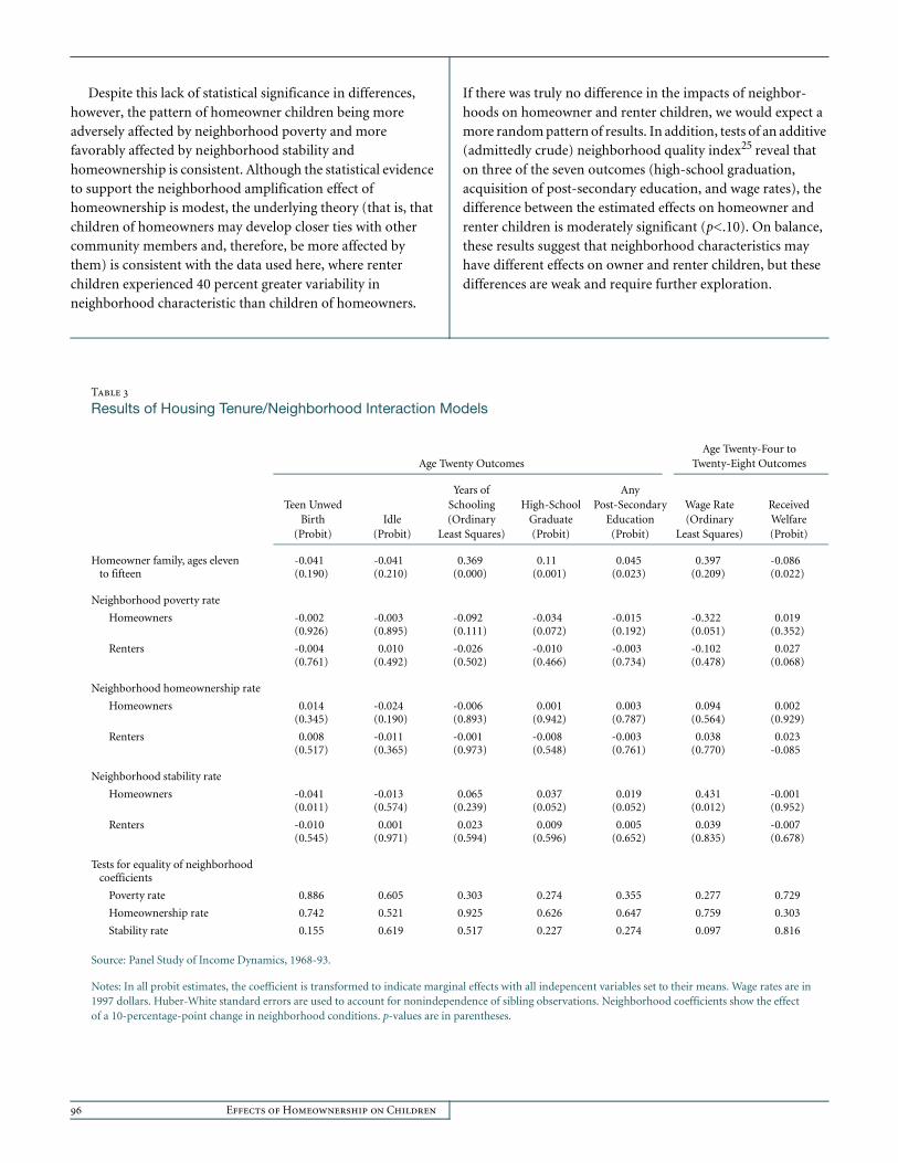
Table 3 shows the results for models testing the interaction of tenure status and neighborhoods.24 The indirect effects models

imposed the assumption that neighborhood characteristics have identical effects on children of homeowners and renters. In the present results, this assumption is relaxed; that is, in the interaction models, the effects of homeownership are allowed to depend upon characteristics of the neighborhood.

The key result of these models is that homeownership does not buffer children against the deleterious effects of bad neighborhoods. If anything, the pattern of results points in the opposite direction—toward an amplification effect. Homeowner children appear to be more adversely affected by neighborhood poverty than renter children, and to benefit more from neighborhood homeownership and residential stability. Effects of neighborhood residential stability, in particular, appear to be better for children of homeowners than for children of renters.

The first row of coefficients in Table 3 shows that in a neighborhood with average sample characteristics (27 percent poverty, 59 percent homeownership, and 57 percent residential stability), the estimated effects of homeownership are nearly the same as in the direct and indirect effects models. Subsequent rows in the table show how these average effects are modified by neighborhood characteristics. For example, the coefficient on homeownership (first row) in the wage rate model is $0.397. A 10-percentage-point increase in the poverty rate of the neighborhood where the child lived between ages eleven and fifteen is estimated to reduce the early adult wage rate of homeowner children by $0.322 and of renter children by $0.102, with a net difference of $0.22. Thus, homeownership in a neighborhood with a 37 percent poverty rate, rather than the sample mean of 27 percent, would raise a child’s early adult wage rate by $0.177 ($0.397 minus $0.22), rather than $0.397.

Comparing coefficients in this way indicates that neighborhood poverty generally has worse effects on the outcomes of homeowner children than on renter children, and neighborhood homeownership and residential stability generally have better effects. But none of the differences between the estimated effects of neighborhoods on children of homeowners and renters are highly statistically significant. In the strongest case, a 10-percentage-point increase in neighborhood residential stability is associated with a statistically significant $0.43 increase in the wage rates of homeowner children (p<.05), but it has no effect on the wage rates of renter children. However, the difference between these two estimates is statistically significant at only a moderate level (p = .10). In another case, the difference between owner and renter children in the impact of neighborhood residential stability on teen out-of-wedlock childbearing is modest (p =.16). None of the other differences is statistically distinguishable at even this weak level.


Despite this lack of statistical significance in differences, however, the pattern of homeowner children being more adversely affected by neighborhood poverty and more favorably affected by neighborhood stability and homeownership is consistent. Although the statistical evidence to support the neighborhood amplification effect of homeownership is modest, the underlying theory (that is, that children of homeowners may develop closer ties with other community members and, therefore, be more affected by them) is consistent with the data used here, where renter children experienced 40 percent greater variability in neighborhood characteristic than children of homeowners.

If there was truly no difference in the impacts of neighbor-hoods on homeowner and renter children, we would expect a more random pattern of results. In addition, tests of an additive (admittedly crude) neighborhood quality index25 reveal that on three of the seven outcomes (high-school graduation, acquisition of post-secondary education, and wage rates), the difference between the estimated effects on homeowner and renter children is moderately significant (p<.10). On balance, these results suggest that neighborhood characteristics may have different effects on owner and renter children, but these differences are weak and require further exploration.

Table 3

Results of Housing Tenure/Neighborhood Interaction Models



Teen Unwed Birth

(Probit)Idle

(Probit)


Least Squares)


Any Post-Secondary

Education(Probit)

Wage Rate(Ordinary

Least Squares)


Homeowner family, ages eleven to fifteen

-0.041(0.190)

-0.041(0.210)

0.369(0.000)

0.11(0.001)

0.045(0.023)

0.397(0.209)

-0.086(0.022)

Neighborhood poverty rate

Homeowners -0.002(0.926)

-0.003(0.895)

-0.092(0.111)

-0.034(0.072)

-0.015(0.192)

-0.322(0.051)

0.019(0.352)

Renters -0.004(0.761)

0.010(0.492)

-0.026(0.502)

-0.010(0.466)

-0.003(0.734)

-0.102(0.478)

0.027(0.068)

Neighborhood homeownership rate

Homeowners 0.014(0.345)

-0.024(0.190)

-0.006(0.893)

0.001(0.942)

0.003(0.787)

0.094(0.564)

0.002(0.929)

Renters 0.008(0.517)

-0.011(0.365)

-0.001(0.973)

-0.008(0.548)

-0.003(0.761)

0.038(0.770)

0.023-0.085

Neighborhood stability rate

Homeowners -0.041(0.011)

-0.013(0.574)

0.065(0.239)

0.037(0.052)

0.019(0.052)

0.431(0.012)

-0.001(0.952)

Renters -0.010(0.545)

0.001(0.971)

0.023(0.594)

0.009(0.596)

0.005(0.652)

0.039(0.835)

-0.007(0.678)

Tests for equality of neighborhood coefficients

Poverty rate 0.886 0.605 0.303 0.274 0.355 0.277 0.729

Homeownership rate 0.742 0.521 0.925 0.626 0.647 0.759 0.303

Stability rate 0.155 0.619 0.517 0.227 0.274 0.097 0.816


Notes: In all probit estimates, the coefficient is transformed to indicate marginal effects with all indepencent variables set to their means. Wage rates are in 1997 dollars. Huber-White standard errors are used to account for nonindependence of sibling observations. Neighborhood coefficients show the effect of a 10-percentage-point change in neighborhood conditions. p-values are in parentheses.


6. Discussion

6.1 Unmeasured Variable Bias

As discussed earlier, the results presented here could be erroneous if the unmeasured characteristics of families that choose different tenure and neighborhood combinations were driving them. In particular, the concern here is that the homeownership coefficients may have much larger upward biases than the neighborhood coefficients. If so, the findings of the preceding analysis would be spurious. However, previous research indicates that estimates for the effects of homeowner-ship and neighborhoods have roughly the same upward bias. Using instrumental variable techniques, Green and White (1997), Haurin, Parcel, and Haurin (2000), and Aaronson (2000) all find a modest upward bias in homeownership effect estimates, while sibling difference analyses and other attempts to gauge the extent of bias associated with neighborhood effect estimates (Aaronson 1997; Duncan, Connell, and Klebanov 1997) also find a modest upward bias associated with neighborhood poverty. These results suggest that conclusions drawn from the uninstrumented results will be qualitatively

correct, although the point estimates may be overstated. In contrast to other studies of homeownership effects, Harkness and Newman (2002) find that homeownership coefficients are biased downward for children of low-income families; that is, the effects of homeownership are even larger than estimates provided by the uninstrumented models.

6.2 Policy Implications

One possible implication of this analysis is that under certain adverse neighborhood characteristics, homeownership could result in worse, not better, outcomes for children, compared with renting. To gain a sense of what these conditions might be, we used the coefficients from the interaction model results to calculate the effects of homeownership if the three neighbor-hood characteristics considered here were worsened by one standard deviation from their means, both individually and simultaneously, with the results presented in Table 4.26 With one exception—the effect of reduced neighborhood residential stability on earnings—all of the estimated effects of homeownership remain favorable. For educational outcomes and welfare receipt, many of these effects remain statistically significant

Table 4

Effects of Homeownership on Early Adult Outcomes under Different Neighborhood Conditions



Teen Unwed Birth

(Probit)Idle

(Probit)


Least Squares)


Any Post-Secondary

Education(Probit)

Wage Rate(Ordinary

Least Squares)


Poverty rate, increase of one standard deviation

-0.037(0.374)

-0.059(0.248)

0.273(0.054)

0.076(0.103)

0.027(0.351)

0.079(0.850)

-0.097(0.062)

Homeownership rate, decrease of one standard deviation

-0.052(0.335)

-0.015(0.779)

0.379(0.014)

0.092(0.092)

0.035(0.270)

0.284(0.610)

-0.043(0.485)

Residential stability, decrease of one standard deviation

-0.005(0.876)

-0.026(0.562)

0.320(0.006)

0.078(0.066)

0.028(0.270)

-0.049(0.903)

-0.092(0.040)

Worsen all neighborhood features by one standard deviation

-0.013(0.800)

-0.018(0.774)

0.235(0.170)

0.026(0.660)

0.001(0.998)

-0.480(0.412)

-0.061(0.357)


Notes: The table uses the coefficients from the interaction models (in Table 3) to show the estimated effects of homeownership when the neighborhood measures are worsened by one standard deviation from their mean values, both individually and simultaneously. In all probit estimates, the coefficient is transformed to indicate marginal effects with all independent variables set to their means. Wage rates are in 1997 dollars. Huber-White standard errors are used to account for nonindependence of sibling observations. p-values are in parentheses.


near conventional levels when individual neighborhood features are worsened. None remain significant when all neighborhood features are simultaneously worsened by one standard deviation, but these sorts of neighborhood characteristics—a poverty rate of 42 percent, a homeownership rate of 39 percent, and only 46 percent of residents remaining in their dwellings for five years or more—roughly represent the worst quintile of neighborhoods in the sample. It is noteworthy that even with these extremely poor neighborhood characteristics, and under the assumption that owner children are, in fact, more adversely affected by these conditions than renter children, effects of homeownership on children’s outcomes tend to be positive.

6.3 Comparison with the Results of Aaronson (2000)

Because this paper uses a different approach than Aaronson (2000) to examine the role of neighborhood in homeownership effects, it is important to compare results. Although both analyses find that neighborhood residential stability enhances the positive effect of homeownership on children’s outcomes, findings on the effect of neighborhood poverty disagree. Aaronson finds that homeownership has a more positive effect on high-school graduation in low-income neighborhoods; we find that neighborhood poverty reduces the positive effect of homeownership on high-school graduation and other outcomes.27

When we attempt to replicate Aaronson’s results using a sample unrestricted by income, our results are consistent with his: homeownership in a high-poverty neighborhood has a significantly more positive effect on high-school graduation than homeownership in a low-poverty neighborhood. Aaronson’s result therefore appears to be attributable to the inclusion of higher income families in the sample. In our results using the low-income sample, homeownership is estimated to increase the probability of high-school graduation by about 10 percentage points, roughly equal in magnitude to the effect Aaronson finds in low-income neighborhoods. Because the families living in low-income neighborhoods in Aaronson’s sample probably have low incomes themselves and, therefore, roughly match the sample we use, our results are consistent with his. Excluded from our sample are the wealthier families who live in the most affluent neighborhoods and for whom homeownership has no effect on children’s high-school graduation, according to Aaronson’s results. Thus, the difference Aaronson finds in high- versus low-income

neighborhoods may, in fact, be attributable to differences in the type of families that live in such neighborhoods, not the neighborhoods themselves.

6.4 Supplementary Models

Measures of home equity and the family’s history of residential mobility were not included in the foregoing models because they could be affected by homeownership or neighborhood characteristics, as discussed earlier. However, when supplementary models that include these measures were tested, the effects of home equity were not statistically significant for any outcome except wage rates. A history of frequent residential moves was associated with the most adverse effects for outcomes, and these effects were statistically significant for all educational outcomes and for wage rates. Like Aaronson (2000), we find the positive effects of homeownership to be weaker when residential moves are added to the model, which suggests that these effects can be partially attributed to the reduced residential mobility of homeowners. But even after we controlled for residential moves, homeownership continued to exhibit statistically significant (p<.05) favorable effects on all three educational outcomes and on reduced welfare usage. It thus appears that the impacts of homeownership on other features, not simply residential stability, need to be examined in order to explain the beneficial effects of homeownership on children.

7. Conclusions

The key finding of this paper is that homeownership is beneficial to children’s outcomes in almost any neighborhood. However, because better neighborhoods are associated with better outcomes for homeowner children, homeownership in better neighborhoods is an even stronger combination. Residentially stable neighborhoods are particularly beneficial to homeowner children, and low neighborhood poverty also increases the benefits of homeownership. Interestingly, however, the neighborhood homeownership rate has no effect.

Are better neighborhoods also better for renter children? The answer appears to be “no.” One possible explanation is that because renter families move more often, renter children do not develop close ties with others in their community and consequently are influenced less by them. The one compensation


is that distressed neighborhoods may also be less deleterious for them, since renters’ children appear to be influenced less by their neighborhoods—good or bad.

These provocative findings imply that the children of most low-income renters would be better served by programs that help their families become homeowners in their current neighborhoods instead of helping them move to better neighborhoods but remain renters. The best evidence to date on the effects of neighborhoods on renter children comes from the Moving-to-Opportunity (MTO) demonstration program. In the program, one group of families living in public housing in highly distressed neighborhoods was offered a Section 8 certificate, counseling, and assistance to help them move out of public housing and into rental housing in very low-poverty neighborhoods. Another group was offered a Section 8 certificate, but no additional assistance, to move as they chose. This latter group generally moved to somewhat better neighborhoods than those of their former public housing residence, but much worse than the experimental group that received assistance in moving to very low-poverty neighborhoods. The early MTO results demonstrate a variety of benefits to both groups of families moving out of public housing. But it is not yet evident whether the children whose families moved to low-poverty neighborhoods are faring much better than those whose families generally remained in fairly

distressed neighborhoods. For example, Ludwig, Duncan, and Ladd (2001) report significant gains in reading scores for both Section 8 mover groups, whether they moved to a low-poverty neighborhood or not. Thus, while it seems clear that helping families to move out of public housing in highly distressed neighborhoods is beneficial, the MTO research has not yet demonstrated that neighborhoods matter significantly for children of renters.28

The research reported here is only an initial strep toward understanding the role of neighborhood characteristics in the effects of homeownership on children. But the research is limited by its small sample size and methodological issues—including the likelihood of upwardly biased estimates because of failure to control for important family characteristics—that render the results of this analysis extremely tenuous. Further research, preferably using an experimental design, is therefore necessary to measure solidly the relative benefits of homeowning and renting for children with a variety of neighborhood characteristics.

Finally, homeownership may generate broader social benefits beyond its favorable effects on children, such as a more active and informed citizenry (DiPasquale and Glaeser 1999) and more residentially stable neighborhoods. The case for greater investment in homeownership must take this full range of potential benefits into account.


Suppose we want to estimate how the neighborhood poverty rate differentially affects children of homeowners and renters. Some children are always homeowners between ages eleven and fifteen, some are always renters, and some experienced both forms of tenure. One solution might be to specify homeownership as years in a homeowning family and multiplicatively interact this variable with the average neighborhood poverty rate experienced over the period. But for those with mixed tenure, the average neighborhood poverty rate comprises both the neighborhood poverty rate while renting and the neighborhood poverty rate while owning, which are two quantities whose effects we want to estimate separately.

Another solution might be to specify separately the average neighborhood poverty rate/level experienced while owning and the average neighborhood poverty rate experienced while renting. The problem here is that average neighborhood poverty rate while owning (renting) is undefined for renters (owners). To correct for this problem, we can set the average neighborhood poverty rate while owning (renting) to zero for renters (owners) and introduce a dummy variable to control for the fact that this substitution has been made. But the dummy variables introduced also act as indicators of zero and five years of homeownership between ages eleven and fifteen,

which means that the model estimates for the effects of homeownership rely solely upon the relatively few cases with mixed tenure status over the period.

The most likely effect of eliminating from the sample children of mixed tenure status between ages eleven and fifteen would be to overestimate the favorable effects of homeownership on children’s outcomes because homeowner-ship is generally indicative of better household conditions, and families that did not become homeowners until their children were age eleven or older are more likely to have been worse off in financial and other ways compared with families that became homeowners earlier. Likewise, families that were already homeowners and became renters after their children were age eleven or older are likely to be undergoing serious difficulties, such as job loss or divorce. (The question of whether homeownership is good for children in families undergoing serious stress is an important one, but it is not examined here.) Thus, the estimates obtained by eliminating families of mixed tenure status should produce the most favorable picture of homeownership effects on children’s outcomes. Tests of basic models (that is, those without tenure/neighborhood interactions) using the full low-income sample support this expectation.

Appendix A: Discussion of Sample Restrictions and Implications


For intercensus years, we interpolated using the values from the two bracketing decennial censuses; for census years and for cases where the data from only one of the bracketing censuses were available, we used values from a single census. (From 1986 on, the Panel Study of Income Dynamics geocode match provided data from the 1990 census only.) Data from two censuses were used in 79 percent of the cases; one census was used for 21 percent of the cases.

Approximately 68 percent of the two-census interpolations were obtained from tract data alone, 10 percent used ZIP code data alone, and 4 percent used a combination of tract and ZIP code measures. In the remaining 18 percent of the two-census cases, data at the tract or ZIP code level were available for only one of the bracketing censuses. For these, we used the value at

the tract or ZIP code level that was available relative to the minor civil division (MCD) value for that census to impute a tract or ZIP code value for the missing census based on its MCD value. That is, we imputed z1 = Z1 * z2 /Z2, where z1 is the missing ZIP code or tract level datum from census year 1, z2 is the available ZIP code or tract level datum from census year 2, and Z1 and Z2 are the MCD level values. (The MCD corresponds roughly to a township or a quarter of a county. Values for the MCD, or something conceptually similar to it, were available for all years.) About 0.4 percent of two-census interpolations used MCD values for both bracketing census years. Of the single-census cases, 73 percent used tract level data, 21 percent used ZIP code level data, and 6 percent used MCD level values.

Appendix B: Data


AppendixAppendix C: Alternative Probit Estimates

Alternative Probit Estimates for Indirect Effects Model

Teen Unwed Birth

(Probit)Idle

(Probit)


Any Post-Secondary

Education(Probit)


Unfavorable family background

Homeowner family, ages eleven to fifteen -0.057(0.176)

-0.056(0.145)

0.128(0.000)

0.029(0.029)

-0.101(0.007)

Neighborhood poverty rate -0.003(0.879)

0.006(0.715)

-0.017(0.178)

-0.004(0.378)

0.024(0.070)

Neighborhood homeownership rate 0.016(0.324)

-0.020(0.142)

-0.005(0.672)

0.000(0.960)

0.017(0.192)

Neighborhood percentage staying five or more years -0.038(0.041)

-0.006(0.737)

0.020(0.122)

0.007(0.132)

-0.006(0.665)

Favorable family background

Homeowner family, ages eleven to fifteen -0.016(0.403)

-0.014(0.373)

0.076(0.010)

0.096(0.006)

-0.072(0.038)

Neighborhood poverty rate -0.001(0.878)

0.001(0.727)

-0.010(0.216)

-0.013(0.363)

0.017(0.103)

Neighborhood homeownership rate 0.004(0.443)

-0.005(0.362)

-0.003(0.672)

-0.001(0.960)

0.012(0.218)

Neighborhood percentage staying five or more years -0.011(0.340)

-0.001(0.739)

0.012(0.151)

0.023(0.122)

-0.004(0.666)


Notes: In all probit estimates, the coefficients were transformed to indicate marginal effects with all variables set to their means. The table shows how these estimates remain stable with different choices for the values of the independent variables. For the “unfavorable family background” estimates, maternal age at birth was set to fifteen, parental earnings to zero, parental education to no high school, years of childhood welfare usage to 100 percent, and asset income to zero. For the “favorable family background” estimates, maternal age at birth was set to thirty, parental earnings to $30,000 annually, parental education to college, years of childhood welfare usage to zero, and asset income to $1,000 annually. Variables other than those mentioned were set to their means. Wage rates are in 1997 dollars. Huber-White standard errors are used to account for nonindependence of sibling observations. p-values are in parentheses.

Endnotes


1. Distressed neighborhoods are typically defined as those with high

rates of poverty, unemployment, and dependence on public

assistance, though researchers differ in their specific operation-

alizations. Some analysts use an index of factors (for example, the

Ricketts-Sawhill definition of underclass neighborhoods) or factor

analysis scores (for example, the papers collected in Brooks-Gunn,

Duncan, and Aber [1997]). Others rely primarily on the poverty rate,

though the cutoff point for “distress” varies from 20 percent (used by

the census to define poverty areas) to 40 percent. These different

definitions are substantively quite similar, because the factors that

characterize distressed neighborhoods are highly interrelated. Most

researchers rely on census tracts as proxies for neighborhoods.

2. See Sandel et al. (1998) for a discussion of health-threatening

conditions in substandard housing. We are aware of only one study

that investigates the effects of milder forms of physical deprivation on

children’s development. Using the National Longitudinal Survey of

Youth (NLSY) child data set, Mayer (1997) constructs a “housing

environment” index, based on whether the interviewer observed the

respondent’s home to be “dark and perceptually monotonous,”

“minimally cluttered,” or “reasonably clean.” She found almost no

effect of this index on young children’s cognitive test scores or

behavioral problems.

3. Data were tabulated from the 1999 American Housing Survey.

4. The better socioeconomic features of homeowning families may be

another factor explaining the improved outcomes of homeowner

children, but all previous studies control for income and other family

features.

5. This speculation follows from the collective socialization and

epidemic models of neighborhood effects (Jencks and Mayer 1990).

6. Green and White (1997) also examine the effect of homeownership

on teen unwed childbearing in one of the three data sets they consider.

Boehm and Schlottman (1999) simulate the indirect effect of

homeownership on lifetime earnings via its impact on educational

attainment, and they also test whether children of homeowners are

more likely to become homeowners themselves.

7. For a four-person, two-child family, 150 percent of the 2001

poverty line was $26,940.

8. Chow tests confirm structural differences between model estimates

obtained from samples of children from families with incomes below

and above 150 percent of the poverty line, indicating that it is not

appropriate to pool the two samples.

9. Green and White (1997) and Haurin, Parcel, and Haurin (2000)

include some rough proxies for neighborhood characteristics in their

models, but acknowledge weaknesses in these proxies. Aaronson

(2000) examines the interaction effects of homeownership by retesting

models on samples split by residence in high- versus low-income

neighborhoods and in high- versus low-stability neighborhoods. But

this technique could produce misleading results for the interactive

effect of homeownership and neighborhood characteristics if the

difference in neighborhood characteristics experienced by

homeowners and renters was unequally distributed in the split

samples.

10. We also experimented with defining low income as having

parental earnings below the regional median for at least two-thirds of

observed years, using the four census-defined regions. This definition

has the advantage of providing a more geographically balanced

sample. It is also more consistent with definitions of low-income

families used in other housing studies, which are usually based on the

median income of the metropolitan area. However, it does not adjust

for family size as does the poverty formula. The two definitions

produce almost identical results.

11. Two other outcomes—whether there are any, and number of,

hours employed between ages twenty-four and twenty-eight—were

also tested and found to be unaffected by parental homeownership.

Results on these two outcomes are not reported below. Hourly wage

rates were constructed by dividing total earnings by work hours. Six

outliers with calculated wage rates of more than $40 an hour and less

than 300 average annual hours of work were excluded from the wage

rate model.

12. Huber-White standard errors are used because the data include

siblings, which may not be independent.

13. Each of these measures was extracted from the PSID census

geocode and averaged over observed years. Census tract level measures

were available for roughly 70 percent of cases, and ZIP code areas were

available for the remainder. Direct census measures were only

obtained for decennial census years. For intercensus years, we linearly

interpolated between the two closest decennial censuses. For example,

for 1975, we interpolated between the 1970 and 1980 census values for

the tract (or ZIP code area). (Appendix B provides more detail on the

construction of neighborhood measures.)


Endnotes (Continued)

14. That is, each neighborhood variable is transformed by subtracting

off its sample mean.

15. A variety of nonlinear specifications for several of these variables

(such as parental earnings, maternal age when born) were tested and

found to have no impact on the key results, and diagnostics for

colinearity problems with these variables using the techniques of

Belsley, Kuh, and Welsch (1980) revealed no such evidence.

16. Annual city size values were obtained by logarithmically

interpolating between place size values in the two closest decennial

census years.

17. The PSID did not begin collecting detailed data on assets until

1984.

18. Diagnostics revealed no colinearity problems with these

neighborhood variables and the other control variables.

19. Harkness and Newman (2002) find that the positive effects of

homeownership on the educational outcomes of the higher income

group are not sustained when instrumental variable techniques are

used to account for unmeasured family background variables. In

contrast, positive effects of homeownership are sustained in the

low-income sample.

20. The smaller sample for teen unwed births is attributable to missing

data and the restriction of the sample to women. A substantial portion

of the data needed to construct the idleness measure is also missing.

The sample used for the wage rate model is smaller because there are

fewer cohorts with data for ages twenty-four to twenty-eight, when

wage rates were measured, and also because it is restricted to cases with

nonzero work hours. (Six cases with fewer than 300 annual average

work hours and wage rates above $40 per hour were also excluded

from the wage rate sample.)

21. An individual’s average wage rate between ages twenty-four and

twenty-eight is likely to be difficult to measure accurately because

earnings and work hours (from which we constructed the wage rate

variable) can be quite volatile from month to month (Duncan 1988),

and it may be difficult for individuals to recall accurately their wage

rates when surveyed annually (as in the PSID). The variables for teen

unwed childbearing and idleness were also constructed from other,

more basic variables in the PSID, which could also introduce

measurement error.

22. For expository purposes, the coefficients on the neighborhood

variables are scaled to represent the effect of a 10-percentage-point

change.

23. It may be that, by fostering greater residential stability, home-

ownership could play an indirect role in creating neighborhood

characteristics beneficial to children’s development. This role appears

to be weak, however. In supplementary models that exclude neighbor-

hood residential stability, the estimated effects of neighborhood

homeownership are only slightly more favorable than those shown

in Table 2.

24. In these results, all interactions were tested simultaneously, not in

separate models or entered in the same model sequentially.

25. This index was formed by adding the homeownership and

residential stability rates and subtracting the poverty rate.

26. These standard deviations are 14, 20, and 11 percentage points for

the poverty rate, homeownership rate, and residential stability rate,

respectively.

27. These findings can be compared because neighborhood poverty

and income are almost perfectly negatively correlated.

28. Complete documentation of the MTO research to date can be

found at <http://www.mtoresearch.org>.

References


Aaronson, Daniel. 1997. “Sibling Estimates of Neighborhood Effects.”

In Jeanne Brooks-Gunn, Greg J. Duncan, and J. Lawrence Aber,

eds., Neighborhood Poverty: Policy Implications in

Studying Neighborhoods. Vol. 2, 80-93. New York: Russell

Sage Foundation.

———. 2000. “A Note on the Benefits of Homeownership.” Journal

of Urban Economics 47, no. 3 (May): 356-69.

Astone, Nan Marie, and Sarah McLanahan. 1994. “Family Structure,

Residential Mobility, and School Dropout: A Research Note.”

Demography 31, no. 4: 575-84.

Austin, Mark D., and Yoko Baba. 1990. “Social Determinants of

Neighborhood Attachment.” Sociological Spectrum 10: 59-78.

Balfour, Danny L., and Janet L. Smith. 1996. “Transforming Lease-

Purchase Housing Programs for Low-Income Families: Towards

Empowerment and Engagement.” Journal of Urban

Affairs 18, no. 2: 173-88.

Barrett, A. Lee, R. S. Oropes, and James W. Kanan. 1994.

“Neighborhood Context and Residential Mobility.”

Demography 31, no. 2: 249-70.

Belsley, David, Edwin Kuh, and Roy Welsch. 1980. Regression

Diagnostics. New York: Wiley Press.

Blum, Terry C., and Paul W. Kingston. 1984. “Homeownership and

Social Attachment.” Sociological Perspectives 27,

no. 2: 159-80.

Boehm, Thomas P., and Alan M. Schlottman. 1999. “Does Home

Ownership by Parents Have an Economic Impact on Their

Children?” Journal of Housing Economics 8: 217-22.

Brooks-Gunn, Jeanne, Greg J. Duncan, and J. Lawrence Aber, eds. 1997.

Neighborhood Poverty: Context and Consequences for

Children. Vol. 1. New York: Russell Sage Foundation.

Conley, Dalton. 1999. Being Black, Living in the Red: Race,

Wealth, and Social Policy in America. Berkeley, Calif.:

University of California Press.

DiPasquale, Denise, and Edward L. Glaeser. 1999. “Incentives and

Social Capital: Are Homeowners Better Citizens?” Journal of

Urban Economics 45: 354-84.

Duncan, Greg J. 1988. “The Volatility of Income over the Life-

Course.” In Paul Baltes, David Featherman, and Richard Lerner,

eds., Life Span Development and Behavior. Vol. 9, 317-58.

Hillsdale, N.J.: Erlbaum.

Duncan, Greg J., James Connell, and Pamela Klebanov. 1997.

“Conceptual and Methodological Issues in Estimating the Causal

Effects of Neighborhoods and Family Conditions on Individual

Development.” In Jeanne Brooks-Gunn, Greg J. Duncan, and

J. Lawrence Aber, eds., Neighborhood Poverty: Context and

Consequences for Children. Vol. 1, 219-50. New York:

Russell Sage Foundation.

Duncan, Greg J., and Stephen W. Raudenbusch. 1998. “Neighborhoods

and Adolescent Development: How Can We Determine the

Links?” Paper presented at the symposium “Does It Take a Village?

Community Effects on Children, Adolescents, and Families.”

Pennsylvania State University, November 5-6.

Ellen, Ingrid Gould, and Margery Austin Turner. 1997. “Does

Neighborhood Matter? Assessing Recent Evidence.” Housing

Policy Debate 8, no. 4: 833-66.

Fitzgerald, John, Peter Gottschalk, and Robert Moffitt. 1998a. “An

Analysis of Sample Attrition in Panel Data: The Michigan Panel

Study of Income Dynamics.” Journal of Human Resources 33,

no. 2: 251-99.

———. 1998b. “An Analysis of the Impact of Attrition on the Second

Generation of Respondents in the Michigan Panel Study of Income

Dynamics.” Journal of Human Resources 33, no. 2: 300-44.

Galster, George C. 1987. Homeowners and Neighborhood

Reinvestment. Durham, N.C.: Duke University Press.

Gephart, Martha A. 1997. “Neighborhoods and Communities as

Contexts for Development.” In Jeanne Brooks-Gunn, Greg J.

Duncan, and J. Lawrence Aber, eds., Neighborhood Poverty:

Context and Consequences for Children. Vol. 1, 1-43.

New York: Russell Sage Foundation.

Green, Richard K., and Michelle J. White. 1997. “Measuring the

Benefits of Homeowning: Effects on Children.” Journal of

Urban Economics 41, no. 3: 441-61.

References (Continued)


Hanushek, Eric, John Kain, and Steven Rivkin. 1999. “The Cost of

Switching Schools.” Unpublished paper, University of Texas at

Dallas. Available at <http://www.utdallas.edu/research/greenctr/

papers/pdfpapers/paper14.html> (November 17, 2000).

Hanushek, Eric, and John Quigley. 1978. “An Explicit Model of

Intra-Metropolitan Mobility.” Land Economics 54, no. 4: 411-29.

Harkness, Joseph M., and Sandra J. Newman. 2002. “The Differential

Impacts of Homeownership on Children from Low-Income and

Higher Income Families.” Unpublished paper, Johns Hopkins

University Institute for Policy Studies.

Haurin, Donald, Tobey Parcel, and R. Jean Haurin. 2000. “The Impact

of Homeownership on Child Outcomes.” Social Science Research

Network Electronic Paper Collection. Available at <http://

papers.ssrn.com/paper.taf?abstract_id=218969>.

Haveman, Robert, Barbara Wolfe, and James Spaulding. 1991.

“Childhood Events and Circumstances Influencing High-School

Completion.” Demography 28, no. 1: 133-57.

Haveman, Robert, and Barbara Wolfe. 1995. “The Determinants of

Children’s Attainments: A Review of Methods and Findings.”

Journal of Economic Literature 33: 1829-78.

Ioannides, Yannis J., and Kamhon Kan. 1996. “Structural Estimation of

Residential Mobility and Housing Tenure Choice.” Journal of

Regional Science 36, no. 3: 335-63.

Jencks, Christopher, and Susan Mayer. 1990. “The Social Consequences

of Growing up in a Poor Neighborhood.” In Laurence Lynn and

Michael McGeary, eds., Inner-City Poverty in the United

States, 111-86. Washington, D.C.: National Academy Press.

Jordan, Will J., et al. 1996. “Exploring the Causes of Early Dropout

among Race, Ethnic, and Gender Groups.” Youth and

Society 28, no. 1: 62-94.

Kan, Kamhon. 2000. “Dynamic Modeling of Housing Tenure Choice.”

Journal of Urban Economics 46: 46-69.

Kasarda, John, and Morris Janowitz. 1974. “Community Attachment

in Mass Society.” American Sociological Review 39: 328-39.

Ludwig, Jens, Greg J. Duncan, and Helen Ladd. 2001. “The Effect of

MTO on Baltimore Children’s Educational Outcomes.”

Northwestern University/University of Chicago Joint Center for

Poverty Research Poverty Research News 5, no. 1: 13-5.

Mayer, Neil S. 1981. “Rehabilitation Decisions in Rental Housing:

An Empirical Analysis.” Journal of Urban Economics 10,

no. 1: 76-94.

Mayer, Susan. 1997. What Money Can’t Buy: Family Income and

Children’s Life Chances. Cambridge: Harvard University Press.

Moffitt, Robert. 1994. “Welfare Effects on Female Headship with Area

Effects.” Journal of Human Resources 29, no. 2: 621-36.

———. 2001. “Policy Interventions, Low-Level Equilibria, and Social

Interactions.” In Steven Durlauf and Peyton Young, eds., Social

Dynamics, 45-82. Cambridge: MIT Press.

Newman, Sandra J., and Greg J. Duncan. 1979. “Residential Problems,

Dissatisfaction, and Mobility.” Journal of the American

Planning Association 45: 154-66.

Page, Maryann, and Gary Solon. 1999. “Correlations between Brothers

and Neighboring Boys in Their Adult Earnings: The Importance of

Being Urban.” Paper presented at the conference “Neighborhood

Effects on Low-Income Families.” Joint Center for Poverty

Research, Chicago, September 9-10.

Quigley, John, and Daniel Weinberg. 1977. “Intra-Urban Residential

Mobility: A Review and Synthesis.” International Regional

Science Review 2, no. 2: 41-66.

Rohe, William M., and Victoria Basolo. 1997. “Long-Term Effects of

Homeownership on the Self-Perceptions and Social Interaction of

Low-Income Persons.” Environment and Behavior 29, no. 6:

793-819.

Rohe, William M., and Michael A. Stegman. 1994. “The Impacts of

Homeownership on the Self-Esteem, Perceived Control, and Life

Satisfaction of Low-Income People.” Journal of the American

Planning Association 60, no. 1: 173-84.

References (Continued)


Rohe, William M., and Leslie S. Stewart. 1996. “Homeownership and

Neighborhood Stability.” Housing Policy Debate 7, no. 1:

37-81.

Rossi, Peter H., and Eleanor Weber. 1996. “The Social Benefits of

Homeownership: Empirical Evidence from National Surveys.”

Housing Policy Debate 7, no. 1: 1-35.

Sampson, Robert J. 1988. “Local Friendship Ties and Community

Attachment in Mass Society: A Multilevel Systemic Model.”

American Sociological Review 53: 766-79.

Sampson, Robert J., Stephen W. Raudenbusch, and Felton Earls. 1997.

“Neighborhoods and Violent Crime: A Multilevel Study of

Collective Efficacy.” Science 277: 918-23.

Sandel, Megan, Joshua Sharfstein, Seth Kaplan, Tracy King, and Mary

Pulaski. 1998. “Not Safe at Home: How America’s Housing Crisis

Threatens the Health of Its Children.” Boston Medical Center and

Children’s Hospital Doc4Kids Project report. Available at

<http://www.bmc.org/program/doc4kids/contents.htm>.

Sherraden, Michael. 1991. Assets and the Poor: A New American

Welfare Policy. Armonk, N.Y.: M. E. Sharpe.

Spivack, Richard. 1991. “Determinants of Housing Maintenance and

Upkeep: A Case Study of Providence, Rhode Island.” Applied

Economics 23: 639-46.

U.S. Department of Housing and Urban Development. 2000. “Cuomo

Sets Goal of Boosting Black and Hispanic Homeownership above

50 Percent in Three Years.” Available at <http://www.hud.gov:80/

pressrel/pr00-132.html>.

Zabel, Jeffry E. 1998. “An Analysis of Attrition in the Panel Study of

Income Dynamics and the Survey of Income and Program

Participation with an Application to a Model of Labor Market

Behavior.” Journal of Human Resources 33, no. 2: 479-506.

The views expressed are those of the authors and do not necessarily reflect the position of the Federal Reserve Bank of New York or the Federal Reserve System. The Federal Reserve Bank of New York provides no warranty, express or implied, as to the accuracy, timeliness, completeness, merchantability, or fitness for any particular purpose of any information contained in documents produced and provided by the Federal Reserve Bank of New York in any form or manner whatsoever.

Effects of Homeownership on Children: The Role of ...€¦ · Neighborhood Characteristics and...

Documents

Transcript of Effects of Homeownership on Children: The Role of ...€¦ · Neighborhood Characteristics and...

References

FRBNY Economic Policy Review / June 2003 105