Graduate Theses, Dissertations, and Problem Reports

2006

Effects of duty cycles on diesel engine component life estimation Effects of duty cycles on diesel engine component life estimation

Dave Jayasinghe West Virginia University

Follow this and additional works at: https://researchrepository.wvu.edu/etd

Recommended Citation Recommended Citation Jayasinghe, Dave, "Effects of duty cycles on diesel engine component life estimation" (2006). Graduate Theses, Dissertations, and Problem Reports. 1733. https://researchrepository.wvu.edu/etd/1733

This Thesis is protected by copyright and/or related rights. It has been brought to you by the The Research Repository @ WVU with permission from the rights-holder(s). You are free to use this Thesis in any way that is permitted by the copyright and related rights legislation that applies to your use. For other uses you must obtain permission from the rights-holder(s) directly, unless additional rights are indicated by a Creative Commons license in the record and/ or on the work itself. This Thesis has been accepted for inclusion in WVU Graduate Theses, Dissertations, and Problem Reports collection by an authorized administrator of The Research Repository @ WVU. For more information, please contact researchrepository@mail.wvu.edu.

EFFECTS OF DUTY CYCLES ON DIESEL ENGINE COMPONENT LIFE ESTIMATION

Dave S. Jayasinghe

Thesis submitted to the College of Engineering and Mineral Resources

At West Virginia University

In partial fulfillment of the requirements For the degree of

Master of Science

In Mechanical Engineering

Mridul Gautam, Ph.D., Chairman Natalia Schmid, Ph.D. W. Scott Wayne, Ph.D.

Department of Mechanical and Aerospace Engineering

Morgantown, West Virginia 2006

Keywords: Duty Cycle, Diesel, Cylinder Pressure, Life Model Copyright 2006 Dave S. Jayasinghe

Effects of Duty Cycles on Diesel Engine Component Life Prediction

Dave S. Jayasinghe

ABSTRACT Engine manufactures have relied on over designed of engines and performance testing to ensure product reliability. The efforts to maximize efficiency and to predict performance characteristics have evoked an interest to study the in-cylinder pressure throughout the respective duty cycle. The duty cycle of an engine is defined as the history of speed and load conditions over which the engine operates in a specific application. Understanding the transient on-road diesel engine duty cycles has been one of major goals for the engine developers. To date there have not been any research performed to identify a wide variety of on-road diesel engine duty cycles. One of the world largest diesel engine manufactures, Cummins Inc., had interest in developing and understanding how the effective life of a diesel engine component is related to its duty cycle. West Virginia University Engine and Emissions Research Laboratory (EERL) was commissioned to conduct this study. The objective of this study is to create a mathematical model that predicts the effective life of diesel engine components with respect to its operational duty cycle. In particular, power cylinder components were considered along with the variations of in-cylinder pressure. Four different duty cycles were evaluated in this study: a concrete mixer, heavy hauler, dump truck, and a transit bus. In-cylinder pressure data for all four duty cycles were statistically analyzed using the tools from non-parametric function and regression analysis. A mathematical model that predicts the power cylinder component lives was created. Mimicking the infield operation, heavy hauler displays the minimum power cylinder component life, while concrete mixer has the maximum life. Ultimately, this mathematical model will enable the engine manufactures to produce more cost effective components for different duty cycle applications, while fulfilling the customer requirements.

ACKNOWLEDGEMENTS

As I write the final chapters at my beloved WVU, I’m compelled to thank a lot

people that made this journey possible. Not for these generous souls I would have not

been the person that I’m today. First and foremost I have to express my deepest gratitude

to Dr. Mridul Gautam. You have been an advisor, a teacher, a friend and a brother to me.

Thank you so much for your guidance, support, believing in me and always been there

for me. Also, my sincere appreciation goes to Dan Carder, who was my direct supervisor

and a great friend. Thanks for your advice, humor and support in and out of the college.

Without Dan, I wouldn’t have ever learned the simplest way of loading a boat on to a

trailer. Thanks for those great memories. The same goes to Tom Spencer and Richard

Atkinson, for all your help and making my life at EERL more pleasurable.

Next, I need to offer my genuine gratitude for the extraordinary support of Dr.

Natalia Schmid. Thanks for all you time and effort towards the fulfillment of my masters

project. Also, I would like to thank the faculty members Dr. Scott Wayne, Dr. Nigel

Clark, Dr. Larry Banta, Dr. Jacky Prucz, Dr. Giampiero Campa and Dr. Greg Thompson

for supporting me in various ways towards the completion of my academics. I would also

like to take this opportunity to thank Mr. Ric Kline and other engineers from Cummins

Inc., in believing me and funding the project and helping us though out all the obstacles.

Also, a group that I can never forget, the staff of our great department, Wes

Riddle, Ryan Barnett, Jean Kopasko, Marilyn Host, Fern Wood, Debbie Willis, Ron

Jarrett, Byron Rapp, Chuck Coleman, Jason England and Ted Christian. You guys made

my life gratifying every second I worked with you all and I’m greatly appreciative of

that.

iii

Raffaello Ardanese, Sam George and Xiaohan Chen, I’m deeply appreciative of

all the time and effort you guys spent making this project a success. I would never forget

all the good times we had working together on this project. Thanks to my contemporaries

– Aaron, Michelangelo, Josh, Chamila, Aseem, Karthik, Ben, Bobby, Mohan, Shashi,

Glenn, Nate, Ram, Guru, Ravi, Hemanth, Mahesh, Viney, Sier, Nick and John. You guys

are awesome and thanks for all the great memories in Morgantown.

Finally, I must reserve my deepest thanks to my family. The support and love that

I received from my parents who are also my role models is the foundation for any success

that I have achieved. From the day I was born, Thaththi and Ammi, you showed me the

light, gave me the courage and hope, taught me patience and provided me with

spirituality, stood next to me like a pillar, sheltered me from sun and rain and gave me the

ultimate, the best parents any son could ever wish for. Also, my loving sister you are so

awesome, and can’t dream of having anyone better than you. Shilpani, my lovely fiancée,

thank you so much for been there encouraging and supporting me every step of the way.

Can’t say enough of all four of you and I’m greatly appreciative of the gift of you that

god have given to me. Also, I want to thank all four of my grand parents, aunt Ruth, little

brothers Prabash and Teddy and my extended family for been who you are.

“Let us rise up and be thankful, for if we didn't learn a lot today, at least we learned a little, and if we didn't learn a little, at least we didn't get sick, and if we got sick, at least

we didn't die; so, let us all be thankful.” Venerable Load Buddha

iv

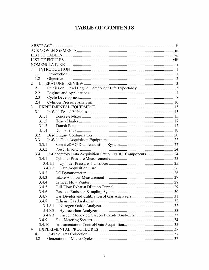
TABLE OF CONTENTS

ABSTRACT........................................................................................................................ ii ACKNOWLEDGEMENTS............................................................................................... iii LIST OF TABLES............................................................................................................ vii LIST OF FIGURES ......................................................................................................... viii NOMENCLATURE ........................................................................................................... x 1 INTRODUCTION ...................................................................................................... 1

1.1 Introduction......................................................................................................... 1 1.2 Objective ............................................................................................................. 2

2 LITERATURE REVIEW ......................................................................................... 3 2.1 Studies on Diesel Engine Component Life Expectancy ..................................... 3 2.2 Engines and Applications ................................................................................... 7 2.3 Cycle Development............................................................................................. 8 2.4 Cylinder Pressure Analysis ............................................................................... 10

3 EXPERIMENTAL EQUIPMENT............................................................................ 15 3.1 In-field Tested Vehicles.................................................................................... 15

3.1.1 Concrete Mixer ......................................................................................... 15 3.1.2 Heavy Hauler ............................................................................................ 17 3.1.3 Transit Bus ................................................................................................ 17 3.1.4 Dump Truck .............................................................................................. 19

3.2 Base Engine Configuration ............................................................................... 20 3.3 In-field Data Acquisition Equipment................................................................ 22

3.3.1 Somat eDAQ Data Acquisition System.................................................... 22 3.3.2 Power Inverter........................................................................................... 24

3.4 In-Laboratory Data Acquisition Setup – EERC Components .......................... 24 3.4.1 Cylinder Pressure Measurements.............................................................. 25

3.4.1.1 Cylinder Pressure Transducer ............................................................... 25 3.4.1.2 Data Acquisition Card........................................................................... 26

3.4.2 DC Dynamometer ..................................................................................... 26 3.4.3 Intake Air flow Measurement ................................................................... 27 3.4.4 Critical Flow Venturi ................................................................................ 28 3.4.5 Full-Flow Exhaust Dilution Tunnel .......................................................... 29 3.4.6 Gaseous Emission Sampling System........................................................ 30 3.4.7 Gas Divider and Calibration of Gas Analyzers......................................... 31 3.4.8 Exhaust Gas Analyzers ............................................................................. 32

3.4.8.1 Nitrogen Oxide Analyzer...................................................................... 32 3.4.8.2 Hydrocarbon Analyzer.......................................................................... 33 3.4.8.3 Carbon Monoxide/Carbon Dioxide Analyzers ..................................... 33

3.4.9 Fuel Metering System............................................................................... 34 3.4.10 Instrumentation Control/Data Acquisition................................................ 35

4 EXPERIMENTAL PROCEDURES......................................................................... 37 4.1 In-Field Data Collection ................................................................................... 37 4.2 Generation of Micro-Cycles ............................................................................. 37

v

4.2.1 Things Considered During Transient Cycle Generation........................... 38 4.3 Engine Set Up and Break-In ............................................................................. 39 4.4 Test Matrix........................................................................................................ 40 4.5 Cylinder Pressure Acquisition .......................................................................... 41

4.5.1 Aspects Considered during Cylinder Pressure Evaluation ....................... 43 4.5.2 Derivation the Volume of Slider-Crank Model ........................................ 45 4.5.3 Work Done by a Piston Cylinder .............................................................. 47 4.5.4 Indicated Mean Effective Pressure ........................................................... 49

4.6 ISM Overhauling Information .......................................................................... 50 5 RESULTS & DISCUSSION .................................................................................... 52

5.1 Introduction....................................................................................................... 52 5.2 Power Cylinder Piston Life Model ................................................................... 52

5.2.1 Cylinder Pressure Evaluation.................................................................... 53 5.2.2 Evaluating the Life Estimation Problem................................................... 57

5.2.2.1 Explain the B-Splines ........................................................................... 58 5.2.2.2 Understanding Radial Basis Functions ................................................. 61 5.2.2.3 Implementation of Radial Basis Function............................................. 63

5.2.3 Numerical Results..................................................................................... 68 6 CONCLUSIONS & RECOMENDATIONS ............................................................ 75

6.1 Conclusions....................................................................................................... 75 6.2 Future Work ...................................................................................................... 76

7 REFERENCES ......................................................................................................... 77 APPENDIX A – Codes Used for Test cell Data Acquisitions and Calculations............. 81

vi

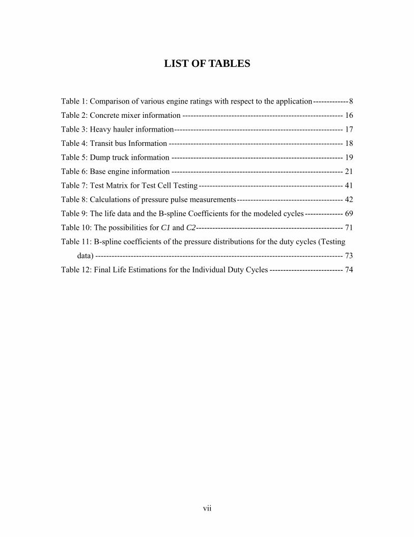
LIST OF TABLES

Table 1: Comparison of various engine ratings with respect to the application-------------8

Table 2: Concrete mixer information ----------------------------------------------------------- 16

Table 3: Heavy hauler information-------------------------------------------------------------- 17

Table 4: Transit bus Information ---------------------------------------------------------------- 18

Table 5: Dump truck information --------------------------------------------------------------- 19

Table 6: Base engine information --------------------------------------------------------------- 21

Table 7: Test Matrix for Test Cell Testing ----------------------------------------------------- 41

Table 8: Calculations of pressure pulse measurements--------------------------------------- 42

Table 9: The life data and the B-spline Coefficients for the modeled cycles -------------- 69

Table 10: The possibilities for C1 and C2------------------------------------------------------ 71

Table 11: B-spline coefficients of the pressure distributions for the duty cycles (Testing

data) ------------------------------------------------------------------------------------------- 73

Table 12: Final Life Estimations for the Individual Duty Cycles --------------------------- 74

vii

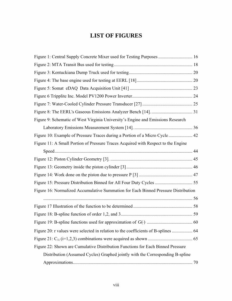
LIST OF FIGURES

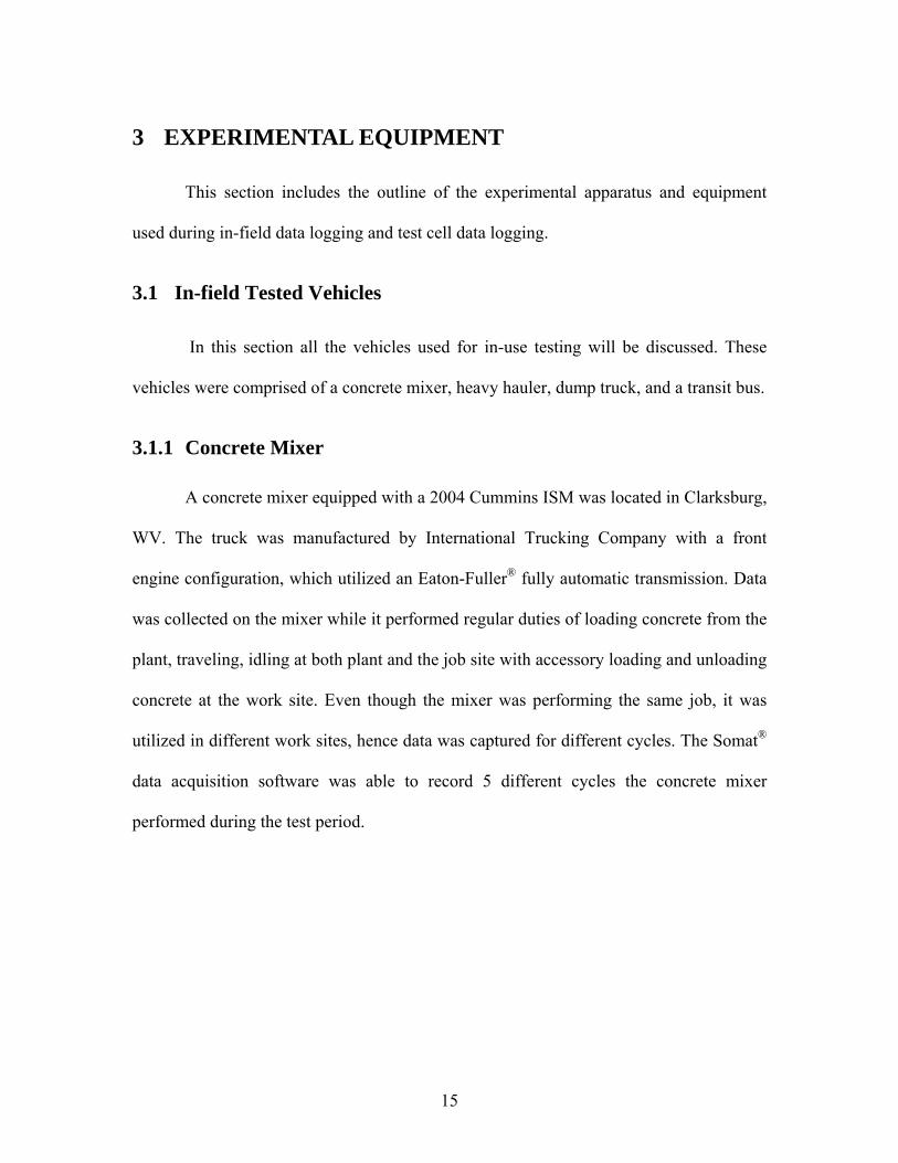
Figure 1: Central Supply Concrete Mixer used for Testing Purposes .............................. 16

Figure 2: MTA Transit Bus used for testing..................................................................... 18

Figure 3: Kentuckiana Dump Truck used for testing........................................................ 20

Figure 4: The base engine used for testing at EERL [18]................................................. 20

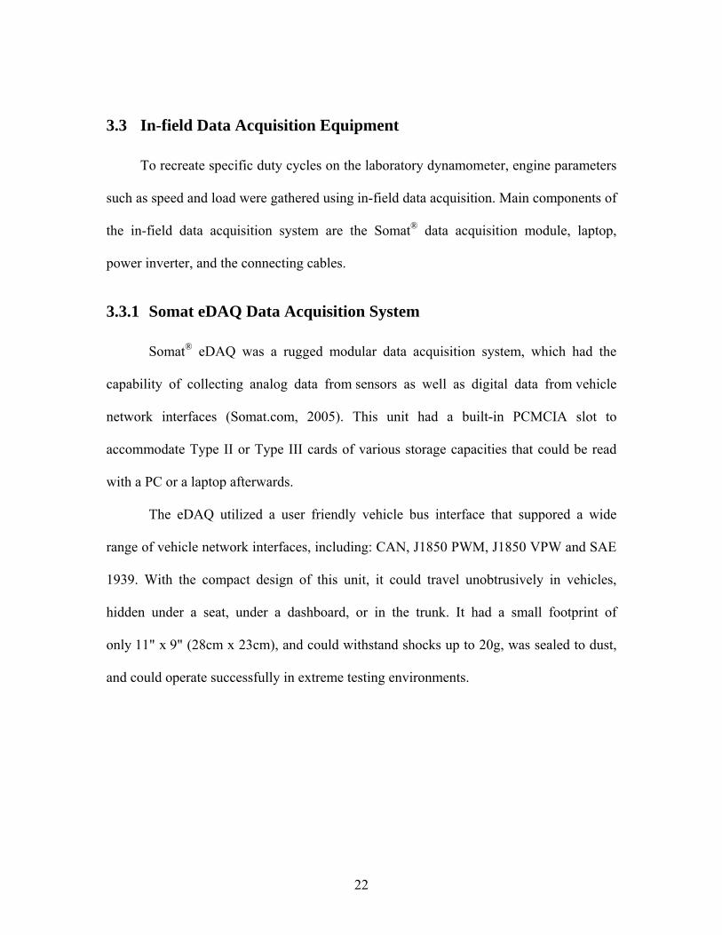
Figure 5: Somat eDAQ Data Acquisition Unit [41] ....................................................... 23

Figure 6 Tripplite Inc. Model PV1200 Power Inverter..................................................... 24

Figure 7: Water-Cooled Cylinder Pressure Transducer [27] ............................................ 25

Figure 8: The EERL's Gaseous Emissions Analyzer Bench [14]. .................................... 31

Figure 9: Schematic of West Virginia University’s Engine and Emissions Research

Laboratory Emissions Measurement System [14]. ................................................... 36

Figure 10: Example of Pressure Traces during a Portion of a Micro Cycle ..................... 42

Figure 11: A Small Portion of Pressure Traces Acquired with Respect to the Engine

Speed......................................................................................................................... 44

Figure 12: Piston Cylinder Geometry [3]. ........................................................................ 45

Figure 13: Geometry inside the piston cylinder [3] .......................................................... 46

Figure 14: Work done on the piston due to pressure P [3] ............................................... 47

Figure 15: Pressure Distribution Binned for All Four Duty Cycles ................................. 55

Figure 16: Normalized Accumulative Summation for Each Binned Pressure Distribution

................................................................................................................................... 56

Figure 17 Illustration of the function to be determined .................................................... 58

Figure 18: B-spline function of order 1,2, and 3............................................................... 59

Figure 19: B-spline functions used for approximation of ( )G ⋅ ........................................ 60

Figure 20: r values were selected in relation to the coefficients of B-splines .................. 64

Figure 21: C1i (i=1,2,3) combinations were acquired as shown ....................................... 65

Figure 22: Shown are Cumulative Distribution Functions for Each Binned Pressure

Distribution (Assumed Cycles) Graphed jointly with the Corresponding B-spline

Approximations......................................................................................................... 70

viii

Figure 23: Shown are Cumulative Distribution Functions for Each Binned Pressure

Distribution (Acquired Duty Cycles) Graphed jointly with the Corresponding B-

spline Approximations. .................................................................................. 72

ix

NOMENCLATURE

AC Alternating Current

BMEP Break Mean Effective Pressure

C-EGR Cooled Exhaust Gas Recirculation

CAN Controller Area Network

CFR Codes of Federal Regulation

CFV Critical Flow Venturi

CVS Constant Flow Sampler

DC Direct Current

DFMEA Design Failure Modes and Effects Analysis

D.I. Direct Injection

ECM Engine Control Module

EERL Engine and Emission Research Laboratory

EPA Environmental Protection Agency

FMEP Frictional Mean Effective Pressure

FTP Federal Transient Procedure

GCS Governor Central Speed

GVWR Gross Vehicle Weight Rating

HFID Heated Flame Ionization Detector

HP Horse Power

IMEP Indicated Mean Effective Pressure

LEF Laminar Flow Element

MEMS Mobile Emissions Monitoring Systems

x

NDIR Non-Dispersive Infrared

NIST National Institute of Standards and Technology

NTE Not-To-Exceed

PCMCIA Personal Computer Memory Card International Association

PFMEA Performance Failure Modes and Effects Analysis

PMEP Pumping Mean Effective Pressure

RBF Radial Basis Function

RPS Revolutions Per Second

RTD Resistive Temperature Device

SAE Society of Automotive Engineers

SCFM Standard Cubic Feet per Minute

SOI Start of Injection

T.D.C. Top Dead Center

UZAM Ultra Zero Air Monitoring

VGT Variable Geometry Turbocharger

WVU West Virginia University

xi

1 INTRODUCTION

1.1 Introduction

Engine manufactures have relied on over-designed engines and performance

testing to ensure product reliability. The effort to maximize efficiency and to predict

performance characteristics have evoked an interest to study the in-cylinder pressure

throughout the respective duty cycles. The duty cycle of an engine is defined as the

history of speed and load conditions over which the engine operates in a specific

application. The different speed and load combinations, the amount of time the engine

spends at those speed and load combinations, and how the engine transitions from one

speed and load combination to another are all key elements of the duty cycle.

Understanding the transient on-road diesel engine duty cycles was a major goal

for the engine developers. One of the world’s largest diesel engine manufacturers,

Cummins Inc., had interest in developing and understanding how the effective life of a

diesel engine component would vary according to its duty cycle. West Virginia

University Engine and Emissions Research Laboratory (EERL) was commissioned to

conduct a study in order to identify these component life predictions.

For this study, a Cummins ISM post-2002 on-road engine was selected. The

selection of the ISM was based upon its versatility and use in on-road applications. This

10.9 liter diesel engine with ratings varying from 280-450 hp, is used in a wide variety of

applications such as line haul trucks, dump trucks, transit buses, concrete mixers, delivery

trucks, recreational vehicles and emergency vehicles.

1

This study comprised of three distinct phases. Phase I involved acquisition of

ECM – broadcast torque, speed and other engine parameters from infield vehicles over

their regular duty cycles. Phase II entailed collection of data on in-cylinder pressure and

other various engine design parameters in an engine dynamometer test cell. During Phase

II the in-laboratory testing was conducted on a Cummins ISM 2004 current product

engine equipped with Cooled Exhaust Gas Recirculation (C-EGR) and the latest ECM

(CM 875). All the engine dynamometer test cell work was conducted at WVU EERL.

Phase III entailed analysis, documentation, and interpretation of data, which was

collected in Phase II.

How the engine duty cycle impacts the life of various diesel engine components is

not well understood or quantified. As the first step in understanding component life,

diesel engine in-cylinder pressure related components were selected. Then, failure and

warranty data were gathered from the component manufacturers. Using manufacturer

data as a model, calculations were performed to evaluate effective life for gathered duty

cycle data.

1.2 Objective

Engine design parameters for multiple duty cycles are essential for ensuring

longevity of engine components. The objective of the study was to predict the life of in-

cylinder pressure related components of a heavy-duty diesel engine using in-cylinder

pressure data. The range over which the in-cylinder pressure operates as a function of

duty-cycle was evaluated to aid component design. This understanding will significantly

minimize the production costs of next generation engines by discounting the engineering

practice of overrating an engine for a certain application.

2

2 LITERATURE REVIEW

This chapter contains a review of published literature on procedures and

methodologies, which have been used in diesel engine duty cycle studies. A more in-

depth review will be done on diesel engine component life expectancy, cylinder pressure

analysis and test cycle generation. A portion of this review discusses previous studies

performed at WVU and information from various engine manufacturers regarding engine

ratings and configurations.

2.1 Studies on Diesel Engine Component Life Expectancy

This section discusses published material on component life expectancy related to

diesel engines. A fewer studies have been performed with regard to other aspects of

diesel engines. Most of the studies involve a mathematical model or a probabilistic

approach based upon field tests.

A method of estimating product durability requirements was reported by Aldridge

(2004). According to this method an understanding of the vehicle usage is a key element

in the general process of defining the product durability requirements.

This method was directed towards virtual testing, in order to analytically

determine product failure distributions, and also create product life distributions. Ability

to predict product life distributions would enhance the life estimations of a certain

product.

Prior to testing, the author conducted a review of Design Failure Modes and

Effects Analysis (DFMEA) and Process Failure Modes and Effect Analysis (PFMEA) to

recognize the highest risk durability parameters. The review was followed up by an

3

exercise to understand and identify parameters, which influence the engine duty cycles,

and those parameters which combined with environmental and customer inputs drive

product operation and damage criterion.

The research done by Shareef and Karmali (2003), focused on failure of diesel

engines due to collapse of fuel injector cam shafts under high friction and load. Some of

the main reasons for the failure of diesel engine fuel injector cams are surface distresses

involving scuffing, frosting, pitting and high friction. Even though it is hard to quantify

the relationship between relative features of failure, the authors reported that some of

those features are “plastic straining, cyclic softening/hardening, crack

initiation/propagation, impact, skidding, and third body formation”. The objectives of

their study (Shareef and Karmali, 2003) were to examine the untimely failure of fuel

injector cams and verify the pitting life of a cam in terms of injection cycles. This study

also attempted to identify how engine load, speed, number of loading cycles, lubrication

condition, and surface roughness affected the life of the injection cam.

Weibull analysis (Wiebull.com, 2005), also known as life data model is a method

to predict the life of all products in a population by fitting a statistical distribution to life

data from a representative sample of units. This parameterized distribution approximates

important life parameters such as probability of failure at a certain time or a failure rate.

Understanding this method requires collecting life data, selecting a model that

will fit the data and be able to model the useful life, approximating the parameters that

will fit the distribution to the given data, and generating results that will guesstimate the

useful life. Life data means measuring the useful life of a product, which could be

expressed and this could be in miles, hours, cycles or any other relevant parameter.

4

A probability density function is a mathematical model that describes the

distribution of a given amount of data. Weibull probability density has the following

form:

( )1 t

tf t e

ββ γηβ γ

η η

− ⎛ ⎞−−⎜ ⎟⎝ ⎠⎛ ⎞−

= ⎜ ⎟⎝ ⎠

, where

η – describes the bulk of the distribution,

β – describes the shape of the distribution, and

γ – describes the location of the distribution in time.

These parameters control the scale, shape and the location of the Weibull

distribution. This distribution could be utilized in a variety of forms using 1, 2 or 3

parameters. Depending on the life distribution, an analyst could choose the parameters

that will make the function fit closely to the data.

Another method was developed by Aldridge (2003) to predict system reliability

and durability using customer usage data, component malfunction distributions, system

failure criteria, manufacturing dissimilarities, and variations in customer severity.

Weibull and Monte Carlo analysis were used in developing this method. Monte Carlo

analysis resolves a problem by generating a suitable amount of random numbers and

observing the fraction of the numbers obeying some property or properties (Mathworld,

2005). The technique is valuable for obtaining numerical solutions to problems which are

too complicated to resolve analytically. The authors cited the following benefits of

utilizing Weibull and Monte Carlo analysis:

• It could provide the ability to create virtual life distribution models based upon

customer usage and production variation data and able to measure and

analytically assess the models.

5

• It could drastically cut down the product delivery time and create a greater

understanding of key failure mechanisms. It could also predict failure time and

failure distribution for a given assembly.

Even though the number of cycles (initial bound was 100 million cycles for an

accelerated test (Aldridge, 2003)) at peak pressure is the main criteria, other parameters

such as engine loading, speed and system operating pressures were considered.

Understanding all the parameters involved in the failure is best described using a matrix,

and building up relationships for individual parameters such as number of cylinder events

at various speed ranges. This is followed up by identifying the cycling requirements for

an accelerated test. As mentioned above, the cycling requirement has been found to be in

the vicinity of 100 million cycles.

After performing the analysis it was concluded that damage from the accelerated

bench test was inadequate in terms of field testing expectations. The virtual testing

demonstrated only less than half of the damage expected in a real life situation. This

outcome demands for an increase in the number of cycles at a higher pressure level.

It was reported that another benefit of this methodology is the ability to define

better and broader accelerated tests for the future, and develop a comprehensive method

to predict reliability for individual components.

Aldridge (2005) developed another method to predict component life in

conjunction with estimations of failure distributions from available warranty data,

customer usage data, and application specific data. This study tests out reasonable

suspension strategy and time based analysis to predict failure distribution. Since neither

one of those methods yields satisfactory results, a distance based suspension strategy was

6

proposed. By means of Monte-Carlo suspension strategy and mixed Wiebull model they

were able to predict failure rates and yield satisfactory results.

Another study conducted by Aldridge (2005) focused on applying and verifying

probabilistic life prediction, while also designing and verifying components for advanced

diesel engines. Probabilistic life prediction of engine components was done using two

parameter Weibull distributions along with maximum likelihood estimation. A dynamic

fatigue test (500-hour rig test) was performed in order to gather sample data for the life

prediction.

2.2 Engines and Applications

This study was conducted on a Cummins ISM 10.9 Liter diesel engine, which was

equipped with a Cooled Exhaust Gas Recirculation (CEGR) unit. Considering the on-

road market, this engine has been the most versatile of all the Cummins engine families

(Cummins.com, 2005). The Cummins ISM engine is utilized in all of the main on-road

heavy-duty truck sectors in the US. The main sectors are on-highway, vocational,

fire/emergency and transit bus. Each of these main categories could be classified into sub

sectors. For an example, concrete mixers and dump trucks are considered to be in the

vocational category. Table 1 illustrates the ratings of similar engine families from a few

diesel engine manufactures. Comparisons were made with Cummins ISM, Caterpillar C-

11 (Cat.com, 2005), Volvo VE D-12 (Volvo.com, 2005), and Detroit Diesel Series 60

(Detroitdiesel.com, 2005). Even though some manufacturers do not manufacture engines

for some of the classifications, they use different engine families to compensate for these

categories. For example, Caterpillar does not have a C-11 engine for the transit bus

sector, but the company manufactures a C-9 engine that is utilized in this category. The

7

table below draws comparisons in rated power (hp) for similar engine families of various

engine manufacturers.

Table 1: Comparison of various engine ratings with respect to the application

Cummins ISM 10.9 L

Caterpillar C 11 11.1 L

Volvo VE D 12 12.1 L

Detroit Diesel Series 60 12.7 L

Engine Ratings in hp

On Highway 280 - 450 305 - 370 365 - 465 330 - 575

Vocational 280 - 450 305 - 370 365 - 465 Fire &

Emergency 340 - 500 305 - 370 350 - 550

App

licat

ions

Transit Bus 280 - 330

2.3 Cycle Development

This section discusses the development of duty cycles for the laboratory testing

purposes. The rarity of published data regarding duty cycle generation for on-road

vehicles leads to exploring the sector of off-road vehicles. Nevertheless, the

considerations and methods were discussed below with respect to duty cycle generation

for test cell purposes.

With the initiation of EPA regulatory program (Phase I – Control of exhaust

emissions of non-road diesel engines over 37 kW) actual test cycles were developed for

off-road applications by Ullman et al., (1999). These cycles were developed using actual

in-use speed and load data acquired from an agricultural tractor, a backhoe loader, and a

crawler tractor. After the data acquisition, using an iterative process, chi-square statistical

data were compared to identify representative micro-trips of the in-use operation. For a

specific application the micro-trips were combined to form a test cycle. This test cycle

8

was statistically analyzed relative to the in-use cycle of the same application for the

validation purposes. After the validation process the test cycle was transformed into

speed and torque points of one second interval. With the help of a reference speed, also

known as the Governor Central Speed (GCS), the speed points were normalized.

Equivalently, the Transient Federal Test Procedure (FTP) was used to normalize the

torque points. Following these procedures Ullman et al., (1999) were able to create a test

cycle that was used for in-laboratory assessments.

Gautam and Krishnamurthy (2005) developed a method to produce an engine test

cycle that would represent real-world heavy-duty truck applications. Development and

use of an on-road cycle in a test cell environment helped better understand in-use

emissions during Not-to-Exceed (NTE) zone operation, engine development and ECM

calibrations. This cycle has developed strictly adhering to the current emissions standards

while collecting and analyzing various engine activity and statistical data within real life

operation of a heavy duty-truck.

Prior to the development of the test cycle, the Mobile Emissions Monitoring

System (MEMS) unit was used to gathering engine operating conditions and in-use-break

specific emissions. After testing a vehicle on a mix of driving routes that included inner

city and highway driving, a database was developed using the representative engine

cycles. Then considering all the driving conditions and routes, a test cycle was developed

that was representative of NTE zone operation.

With a sequence of vibration durability tests, Aldridge (1987) compressed

thousands of hours of customer usage data into realistic length laboratory tests.

According to the author, typical U.S. drivers operate engines from 3,000 to 5,000 hours

9

for each 100,000 mile segment. These operational hours are much higher than the typical

dynamometer tests of 100 to 1,000 hours. This makes it critical to determine the time

basis, which is the time that the engine will spend in each speed range during in-house

testing. Hence, slow RPM sweeps during the field testing were ignored since they are

statistically insignificant and engine wear is minimal during these periods.

2.4 Cylinder Pressure Analysis

Understanding cylinder pressure in regards with different duty-cycles played a

critical role during this study. Hence, the following review was done to understand

cylinder pressure measurement techniques, as well as calculations and analysis involving

cylinder pressure.

The research done by Brunt and Platts (1999) focused on errors in gross heat

release calculations performed during in-cylinder pressure data analysis. Heat release

analysis and burn rate analysis using in-cylinder pressure data are critically important in

order to better understand diesel engines.

Heat release in diesel engines is of huge importance, since it has significant

influence on combustion noise, pressure rise rate and NOx emissions. Nevertheless,

misleading results could produce by both erroneous experimental measurements and heat

release models. The traditional single zone first law heat release model could produce

such errors and the author illustrated these errors when using this model to simulate direct

injection diesel engine pressure diagrams. It was shown that the highest uncertainty errors

could be attributed to the assumption of a wrong rate of heat transfer between power

cylinder charge and combustion chamber walls. To avoid this scenario, an alternative

heat release model was proposed, and it resulted in a large improvement in results over a

10

wide range of operating conditions. The alternative heat release model utilized a variable

polytropic index to account for heat transfer, where it was specifically suited for diesel

engines.

Another study conducted by Assanis et al., (2000) is based upon understanding

transient heat release analysis of diesel engines, created a systematic mythology for

performing these transient heat release analysis. The researchers developed a novel

method to infer the mass of air trapped in the cylinder and the mass of fuel injected on a

cycle-by-cycle basis. The cyclic mass of air trapped in the cylinder was found by

accounting for pressure gradients, piston motion & short-circuiting during the valve

overlap period. The cyclic mass of fuel injected was computed from the measured

injector needle pressure history during the injection period. These parameters were then

used in conjunction with cycle-resolved pressure data to accurately define the

instantaneously thermodynamic state of the mixture and to calculate transient heat release

profiles.

It was understood, unlike in the steady-state operation, where standard flow

meters can be used to measure both fuel & air flow rates, during the transient engine

operation, cycle fuel rates need to be resolved at much faster rates, which could be of the

order of fractions of a second. Hence, a method was developed to deduce critical

parameters for transient analysis from available, measured signals. The method involves

determination of the following.

Start of Fuel Injection – Dynamics of Start of Injection (SOI) is inferred from

measuring the fuel injection pressure profile, and processing of the rocker arm strain gage

signals.

11

Cyclic Fuel Mass & Rate of Injection – In this instance, the fuel injection pressure

profile and in-cylinder pressure profile can be understood by processing the rocker arm

strain gain signal which will ultimately help understanding the rate of injection.

Assuming one-dimensional, quasi-steady, incompressible fuel flow through the nozzle,

the instantaneous mass flow rate was deduced with the same pressure profiles.

Trapped Air Mass – Trapped air mass was calculated assuming that the temperature at

the inlet valve closing is equal to that of the air is in the intake manifold. The

determination of trapped air mass experimentally involves 2 stages: (i) when the exhaust

valve(s) are closed & (ii) when the intake & exhaust valves are both open & overlapping.

Finally, it was concluded that the above mentioned transient effects could be

captured only with the above developed method to analyze a long sequence of cycles

under the transient operation conditions.

Williams and Witter (2001) developed a method to identify misfiring cylinders

with the help of crankshaft angular velocity measurements. To identify the misfiring

cylinders, cylinder pressure and cylinder torque were reconstructed using crank shaft

angular velocity. Calculating IMEP for each cylinder with the help of in-cylinder

pressure data enabled creating a linear parameterization between IMEP and cylinder

excitation torque. Once the IMEP was calculated, indicated torque was determined for

each cylinder using swept volume of the cylinder. Then, the indicated torque was used to

identify the presence of misfire, the misfiring cylinders, the degree of misfire, and most

importantly, the faulty cylinders before excessive damage was done.

Rocco (1993) has performed analysis on how the T.D.C. setting error could affect

the direct injection diesel engine in-cylinder pressure data. Since in-cylinder pressure data

12

are critical in calculating IMEP, and rate of heat release as a method to understand

combustion process, it is imperative that T.D.C. setting error be accounted for. The

authors reported that:

• For a D.I. diesel engine, even a small T.D.C. setting error could produce a

wide uncertainty near the Top Dead Center (T.D.C.) where the highest in-

cylinder pressures rise could be seen.

• With a small error at T.D.C., net heat release rate curves can have substantial

differences in shape and value. Also, it is noticed that an error of 1% at T.D.C.

could yield up to 10% variation in the calculation of net heat release.

• Considering the conversion from net heat release analysis to mechanical work

performed, significant error could be seen in the calculation of mechanical

work. Hence, this could hinder the performance evaluation of an engine.

A study conducted at Detroit Diesel Corporation by Brown and Neill (1992)

explains a non-contact method of determining in-cylinder pressure for a reciprocating

engine. This method was based on a pattern recognition technique, and compared the

crankshaft speed fluctuations to known reference patterns.

It was shown that the non-intrusive method of measurement of in-cylinder

pressure with flywheel angular velocity fluctuations can produce an error less than 6% of

the rms value. Alternatively, when the in-cylinder pressure was less than 10% of the

operating condition, this method had only 1% chance of predicting that a faulty cylinder

was healthy.

13

Further, an under fueling cylinder could reduce the peak cylinder pressure on the

healthy cylinders up to 25%. So, indication of a low cylinder pressure doesn’t necessarily

imply that a certain cylinder is faulty.

The research done by Payri et al., (2005) introduced a novel method to analyze in-

cylinder pressure in a direct injection diesel engine. The reasoning behind this was to

decompose the cylinder pressure signal into three regions during the regular engine

operation, which would provide more complete basis for analysis. These regions are

pseudo-motored, combustion and resonance excitation. Since the combustion process of a

DI diesel engine is a significant source of noise, a combustion noise analysis was

performed to validate this method.

The authors showed that, the amount of energy in the resonance signal, compared

to the amount of energy in the pseudo-motored signal tends to be a more relevant

indicator of the in-cylinder pressure relative to the combustion noise. Also, according to

this approach speed and load dissimilarities have been analyzed and proven that the

combustion signal is mostly controlled by the speed, whereas the resonance signal mostly

depends on the engine load. The resonance signal depends on the load mainly due to its

dependence on temperature.

This study was a powerful example of how the combustion process could be

analyzed with alternative methods, such as combustion noise relative to in-cylinder

pressure.

14

3 EXPERIMENTAL EQUIPMENT

This section includes the outline of the experimental apparatus and equipment

used during in-field data logging and test cell data logging.

3.1 In-field Tested Vehicles

In this section all the vehicles used for in-use testing will be discussed. These

vehicles were comprised of a concrete mixer, heavy hauler, dump truck, and a transit bus.

3.1.1 Concrete Mixer

A concrete mixer equipped with a 2004 Cummins ISM was located in Clarksburg,

WV. The truck was manufactured by International Trucking Company with a front

engine configuration, which utilized an Eaton-Fuller® fully automatic transmission. Data

was collected on the mixer while it performed regular duties of loading concrete from the

plant, traveling, idling at both plant and the job site with accessory loading and unloading

concrete at the work site. Even though the mixer was performing the same job, it was

utilized in different work sites, hence data was captured for different cycles. The Somat®

data acquisition software was able to record 5 different cycles the concrete mixer

performed during the test period.

15

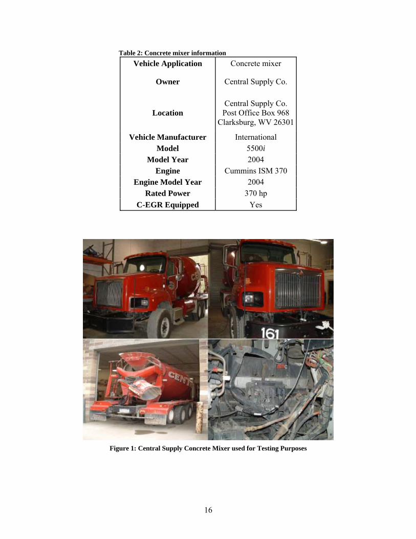
Table 2: Concrete mixer information Vehicle Application Concrete mixer

Owner Central Supply Co.

Location Central Supply Co. Post Office Box 968

Clarksburg, WV 26301

Vehicle Manufacturer International Model 5500i

Model Year 2004 Engine Cummins ISM 370

Engine Model Year 2004 Rated Power 370 hp

C-EGR Equipped Yes

Figure 1: Central Supply Concrete Mixer used for Testing Purposes

16

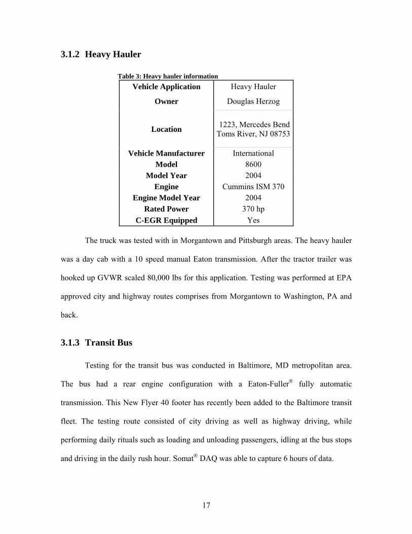
3.1.2 Heavy Hauler

Table 3: Heavy hauler information Vehicle Application Heavy Hauler

Owner Douglas Herzog

Location 1223, Mercedes Bend Toms River, NJ 08753

Vehicle Manufacturer International Model 8600

Model Year 2004 Engine Cummins ISM 370

Engine Model Year 2004 Rated Power 370 hp

C-EGR Equipped Yes The truck was tested with in Morgantown and Pittsburgh areas. The heavy hauler

was a day cab with a 10 speed manual Eaton transmission. After the tractor trailer was

hooked up GVWR scaled 80,000 lbs for this application. Testing was performed at EPA

approved city and highway routes comprises from Morgantown to Washington, PA and

back.

3.1.3 Transit Bus

Testing for the transit bus was conducted in Baltimore, MD metropolitan area.

The bus had a rear engine configuration with a Eaton-Fuller® fully automatic

transmission. This New Flyer 40 footer has recently been added to the Baltimore transit

fleet. The testing route consisted of city driving as well as highway driving, while

performing daily rituals such as loading and unloading passengers, idling at the bus stops

and driving in the daily rush hour. Somat® DAQ was able to capture 6 hours of data.

17

Table 4: Transit bus Information Vehicle Application Transit Bus

Owner Maryland Transit Administration

Location Maryland Transit Administration

6 St. Paul St, Baltimore MD 21202-1614

Vehicle Manufacturer New Flyer Model D40LF

Model Year 2005 Engine Cummins ISM 370

Engine Model Year 2005 Rated Power 370 Hp

C-EGR Equipped Yes

Figure 2: MTA Transit Bus used for testing

18

3.1.4 Dump Truck

The dump truck tested in this study, was located in Clarksville, IN. The vehicle

was used to move earth fill from an excavating site to a near-by dump site. Even though

this wasn’t a lengthy route, the duty cycle comprised of constant loading and unloading

for the entire 10-hour nonstop work shift. The average duty cycle involved loading at the

excavating site, traveling to the dump site, unloading at the dump site, traveling back

empty to the excavating site. The engine was idling while the truck was getting loaded.

The significant difference in this duty cycle was having low engine speeds and high

engine loads for greater amount of time within the operation. The dump truck was

manufactured by International Truck Company and uses a Eaton-Fuller® fully automatic

transmission.

Table 5: Dump truck information

Vehicle Application Dump Truck

Owner Kentuckiyana Trucking Inc.

Location Kentuckiyana Trucking Inc. 380 Emery Ln, Clarksville, IN 47129

Vehicle Manufacturer International

Model 5600i Model Year 2004

Engine Cummins ISM 370 Engine Model Year 2004

Rated Power 370 Hp C-EGR Equipped Yes

19

Figure 3: Kentuckiana Dump Truck used for testing

3.2 Base Engine Configuration

Figure 4: The base engine used for testing at EERL [18]

20

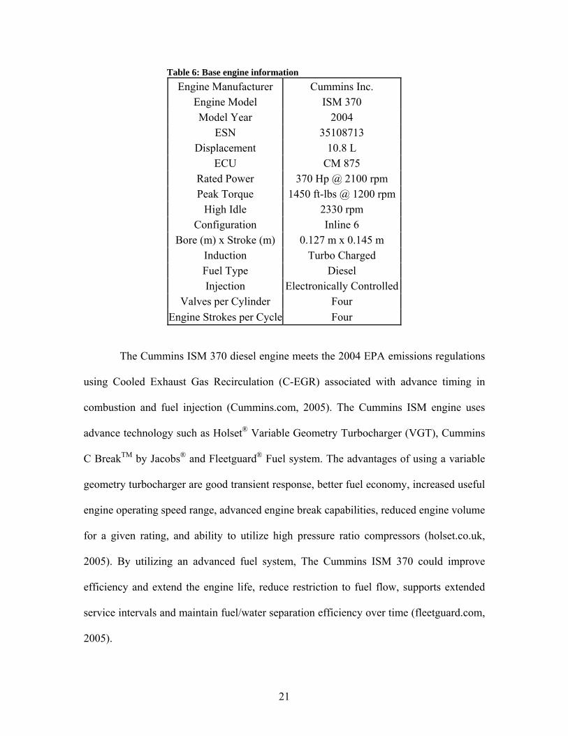
Table 6: Base engine information Engine Manufacturer Cummins Inc.

Engine Model ISM 370 Model Year 2004

ESN 35108713 Displacement 10.8 L

ECU CM 875 Rated Power 370 Hp @ 2100 rpm Peak Torque 1450 ft-lbs @ 1200 rpm

High Idle 2330 rpm Configuration Inline 6

Bore (m) x Stroke (m) 0.127 m x 0.145 m Induction Turbo Charged Fuel Type Diesel Injection Electronically Controlled

Valves per Cylinder Four Engine Strokes per Cycle Four

The Cummins ISM 370 diesel engine meets the 2004 EPA emissions regulations

using Cooled Exhaust Gas Recirculation (C-EGR) associated with advance timing in

combustion and fuel injection (Cummins.com, 2005). The Cummins ISM engine uses

advance technology such as Holset® Variable Geometry Turbocharger (VGT), Cummins

C BreakTM by Jacobs® and Fleetguard® Fuel system. The advantages of using a variable

geometry turbocharger are good transient response, better fuel economy, increased useful

engine operating speed range, advanced engine break capabilities, reduced engine volume

for a given rating, and ability to utilize high pressure ratio compressors (holset.co.uk,

2005). By utilizing an advanced fuel system, The Cummins ISM 370 could improve

efficiency and extend the engine life, reduce restriction to fuel flow, supports extended

service intervals and maintain fuel/water separation efficiency over time (fleetguard.com,

2005).

21

3.3 In-field Data Acquisition Equipment

To recreate specific duty cycles on the laboratory dynamometer, engine parameters

such as speed and load were gathered using in-field data acquisition. Main components of

the in-field data acquisition system are the Somat® data acquisition module, laptop,

power inverter, and the connecting cables.

3.3.1 Somat eDAQ Data Acquisition System

Somat® eDAQ was a rugged modular data acquisition system, which had the

capability of collecting analog data from sensors as well as digital data from vehicle

network interfaces (Somat.com, 2005). This unit had a built-in PCMCIA slot to

accommodate Type II or Type III cards of various storage capacities that could be read

with a PC or a laptop afterwards.

The eDAQ utilized a user friendly vehicle bus interface that suppored a wide

range of vehicle network interfaces, including: CAN, J1850 PWM, J1850 VPW and SAE

1939. With the compact design of this unit, it could travel unobtrusively in vehicles,

hidden under a seat, under a dashboard, or in the trunk. It had a small footprint of

only 11" x 9" (28cm x 23cm), and could withstand shocks up to 20g, was sealed to dust,

and could operate successfully in extreme testing environments.

22

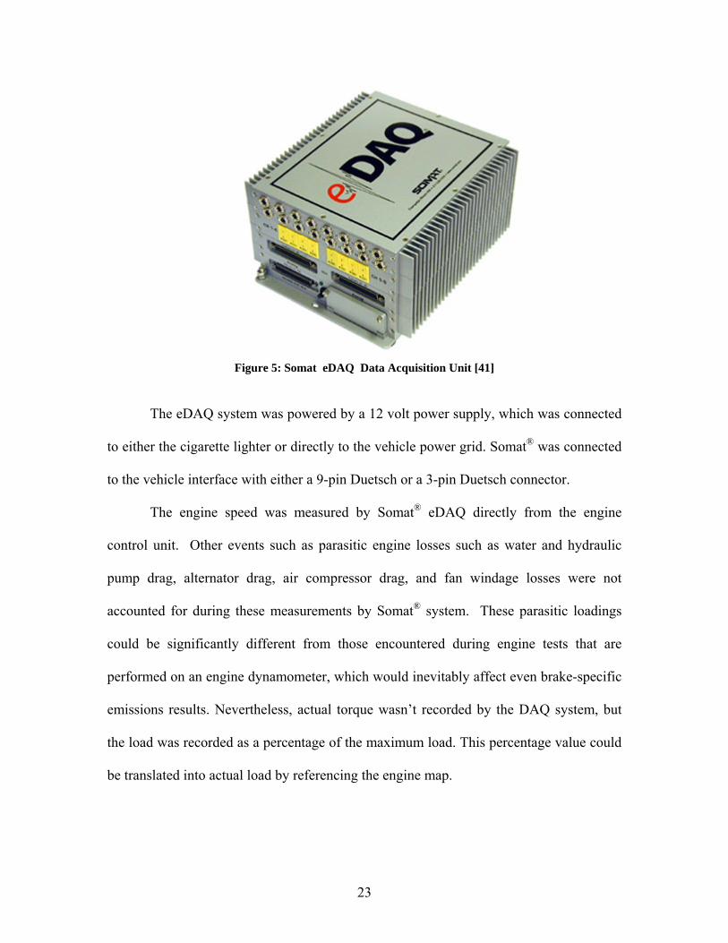
Figure 5: Somat eDAQ Data Acquisition Unit [41]

The eDAQ system was powered by a 12 volt power supply, which was connected

to either the cigarette lighter or directly to the vehicle power grid. Somat® was connected

to the vehicle interface with either a 9-pin Duetsch or a 3-pin Duetsch connector.

The engine speed was measured by Somat® eDAQ directly from the engine

control unit. Other events such as parasitic engine losses such as water and hydraulic

pump drag, alternator drag, air compressor drag, and fan windage losses were not

accounted for during these measurements by Somat® system. These parasitic loadings

could be significantly different from those encountered during engine tests that are

performed on an engine dynamometer, which would inevitably affect even brake-specific

emissions results. Nevertheless, actual torque wasn’t recorded by the DAQ system, but

the load was recorded as a percentage of the maximum load. This percentage value could

be translated into actual load by referencing the engine map.

23

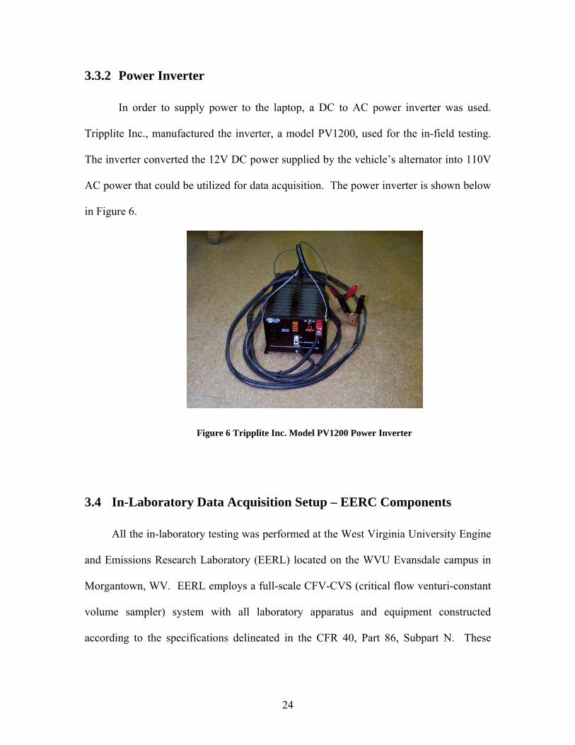
3.3.2 Power Inverter

In order to supply power to the laptop, a DC to AC power inverter was used.

Tripplite Inc., manufactured the inverter, a model PV1200, used for the in-field testing.

The inverter converted the 12V DC power supplied by the vehicle’s alternator into 110V

AC power that could be utilized for data acquisition. The power inverter is shown below

in Figure 6.

Figure 6 Tripplite Inc. Model PV1200 Power Inverter

3.4 In-Laboratory Data Acquisition Setup – EERC Components

All the in-laboratory testing was performed at the West Virginia University Engine

and Emissions Research Laboratory (EERL) located on the WVU Evansdale campus in

Morgantown, WV. EERL employs a full-scale CFV-CVS (critical flow venturi-constant

volume sampler) system with all laboratory apparatus and equipment constructed

according to the specifications delineated in the CFR 40, Part 86, Subpart N. These

24

components will be briefly discussed in this section. Also a schematic of the laboratory

testing setup will be shown in Figure 9.

3.4.1 Cylinder Pressure Measurements

For cylinder pressure acquisition a KISTLER® pressure transducer was used and

for data acquisition a NI® hi-speed daq card was used. A Labview code was written to

facilitate data acquisition and analysis of in-cylinder pressure data (Ardanese, 2005).

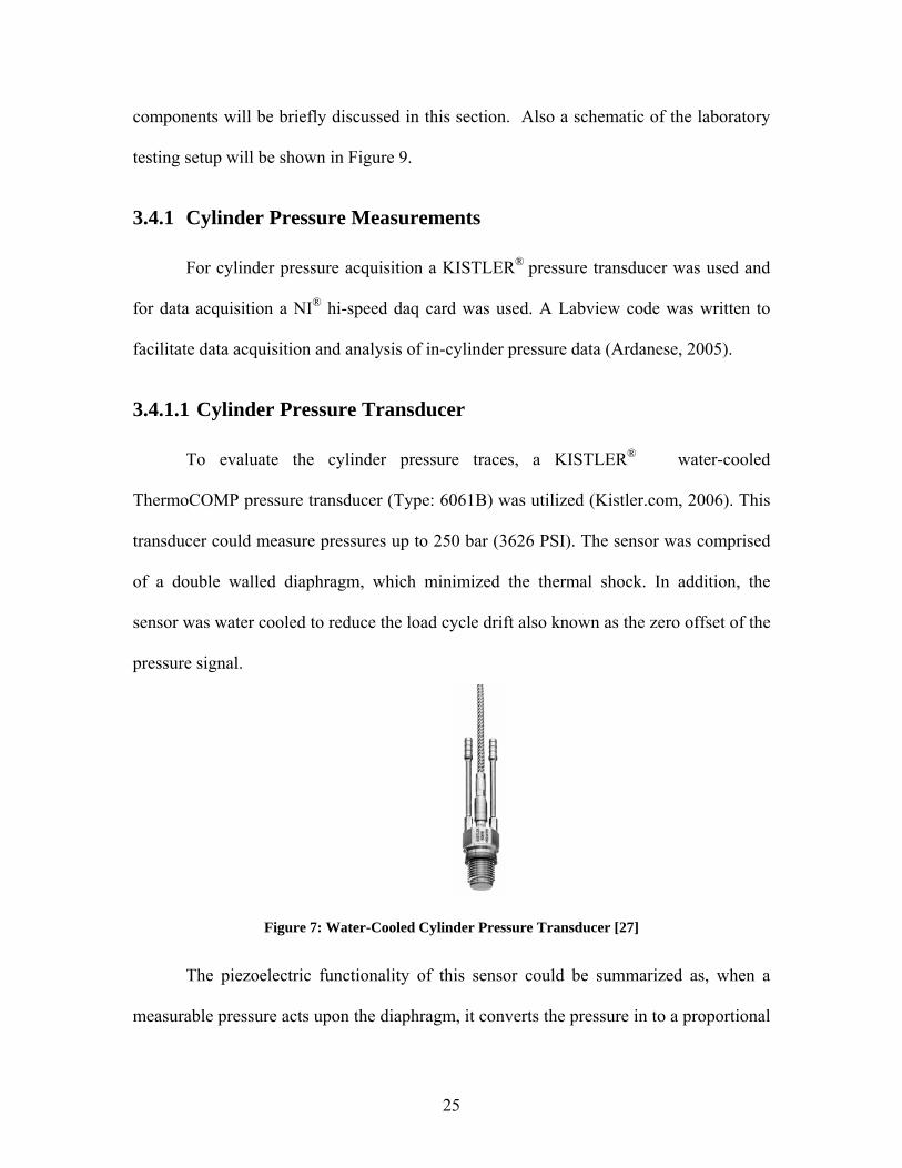
3.4.1.1 Cylinder Pressure Transducer

To evaluate the cylinder pressure traces, a KISTLER® water-cooled

ThermoCOMP pressure transducer (Type: 6061B) was utilized (Kistler.com, 2006). This

transducer could measure pressures up to 250 bar (3626 PSI). The sensor was comprised

of a double walled diaphragm, which minimized the thermal shock. In addition, the

sensor was water cooled to reduce the load cycle drift also known as the zero offset of the

pressure signal.

Figure 7: Water-Cooled Cylinder Pressure Transducer [27]

The piezoelectric functionality of this sensor could be summarized as, when a

measurable pressure acts upon the diaphragm, it converts the pressure in to a proportional

25

force. Then, a quartz packet converts this load into an electrostatic charge, where an

electrode feeds this negative charge into a charge amplifier. Finally the charge amplifier

converts the signal in to a readable positive voltage.

3.4.1.2 Data Acquisition Card

When acquiring cylinder pressure traces roughly around 40 kHz, it was necessary

to utilize a high speed data acquisition card such as a S-Series Multifunction DAQ (250

kS/s, 16-Bit) made by National Instruments (NI.com, 2005). This NI® PCI-6143 daq card

had 8 differential 16-bit analog inputs as well as 8 digital I/O lines and was capable of

simultaneous sampling and high throughput. The NI® PCI-6143 provided a very low cost

per channel while maintaining high dynamic accuracy and simultaneity. During testing,

two digital channels were used for encoder pulses while an analog channel was used for

the pressure transducer signal. A code written in LabVIEW was used since it supported

the platform for NI® PCI-6143 daq card.

3.4.2 DC Dynamometer [Vinay Nagendran, 2003]

EERL employed a GE Model DYC-243 fan cooled, direct current (DC)

dynamometer (power rating of 200 Hp; current rating of 300 amps at 3000 rpm). This

specific dynamometer was capable of absorbing 550 hp and providing up to 500 hp

during motoring of the engine. An electric dynamometer closely resembles the electric

motors in operation. The DC dynamometer consisted of an armature and stator assembly,

which generates the torque. The engine output was measured by a load-cell mounted on

the dynamometer frame and altering the load on the dynamometer also varies the load

applied. The load cell was calibrated by suspending known weights from an arm of

known length, mounted opposite to the load cell. This technique provided tension equal

26

to the maximum value of force reachable by the dynamometer at any given time. Engine

speed was recorded with a digital speed encoder within the dynamometer.

3.4.3 Intake Air flow Measurement

A Meriam Instruments Laminar Flow Element (LFE) was used to quantify the

intake airflow rates. The LFE was made up of a series of small capillary tubes oriented

parallel to the direction of the airflow. The capillary matrix produced a laminar flow of

air from the turbulent flow entering it. A pressure drop was created in the LFE from the

friction of the air passing through the tiny capillaries. A calibration equation was supplied

by Meriam Instruments that helped calibrate the LFE. The absolute temperature and

pressure upstream of the capillary matrix and the pressure downstream of the matrix were

the solitary parameters required for intake volume flow determination and the equation is

shown below (CFR, 2000).

( )2( ) ( ) std

Actualflow

V B P C P µµ

• ⎛ ⎞= × ∆ + × ∆ ×⎜ ⎟⎜ ⎟

⎝ ⎠

Where,

ActualV•

= volume flow rate of air through LFE

B = coefficient supplied by Meriam Instruments

C = coefficient supplied by Meriam Instruments

µstd = standard kinematic viscosity

µflow = actual flow kinematic viscosity

∆P = differential pressure across LFE

A correction factor was used to account for viscosity variations and is as follows:

27

529.67 181.87459.67 ( )oCorrection Factor

T F gµ⎛ ⎞ ⎛

= ×⎜ ⎟ ⎜+⎝ ⎠ ⎝

⎞⎟⎠

⎟⎟⎠

⎞⎜⎜⎝

⎛ ++

⎟⎟⎠

⎞⎜⎜⎝

⎛ ++

=

8.1)(67.4594.110

8.1)(67.45958.14

5.1

FT

FT

go

o

µ

The LFE used for all in-laboratory testing at EERL was a Meriam Model 50MC2-

4 LFE with inside diameter 10.2 cm (4 in.) and maximum flow rate of 11.32 m3/min (400

cfm) [Carder, 1999]. A MKS 223 B differential pressure transducer was used to measure

the differential pressure across the laminar flow element, while absolute upstream

pressure was determined with a Setra Model C280E pressure transducer. The

temperature of the inlet air upstream of the LFE was recorded with a Resistive

Temperature Device (RTD).

3.4.4 Critical Flow Venturi

A CVS system was used to regulate the flow of diluted exhaust gases passing

through the dilution tunnel according to the specifications mentioned in CFR 40. When

the critical flow venturi reached sonic conditions (choked flow); a constant mass flow

rate was maintained in the dilution tunnel. During the sonic operation, flow through the

venturi was a function of the diameter of the throat and the pressure and temperature of

the gas upstream. Pressure data was collected with a Viatran model 1042 AC3AAA20

pressure transducer as the temperature was documented with a resistive temperature

device (RTD). Knowing the absolute temperature and absolute pressure, mass flow rate

was calculated as follows:

28

VK PQT

=

Where,

Q = the flow rate in scfm at standard conditions (20o C and 101.3 Kpa)

Kν = the calibration coefficient of the venturi

P = the absolute pressure at the inlet of the venturi in Kpa

T = the absolute temperature at the inlet of the venturi in oK

3.4.5 Full-Flow Exhaust Dilution Tunnel

Since exhaust emissions testing primarily depends on understanding the effects of

emissions after mixing with the ambient air, it is necessary to simulate “real world”

conditions while acquiring data. Not only does the CVS simulate “real world” conditions

by interacting with dilution air, it also quenches post-cylinder combustion reactions and

decreases the exhaust gas dew point to hamper condensation. Exhaust line quenching is

necessary to prevent measurement inconsistencies of emission. Additionally, by

eliminating water in the sampling stream, it reduces the risk of certain gaseous

components are being soluble such as nitrogen dioxide (NO2), which could unfavorably

influence measurement accuracy.

The EERL utilized a full-flow dilution tunnel for conducting emissions research.

A full-flow dilution tunnel collects the entire exhaust stream from the engine and mixes

with the clean ambient air. The full-flow system housed at EERL was designed and

operated in-accordance with specifications outlined in CFR 40, Part 86, Subpart N. This

system is based upon the CFV-CVS principle. This method embarks a large centrifugal

blower that draws the diluted exhaust gas mixture from the tunnel through critical flow

29

venturi. The primary dilution tunnel was constructed with stainless steel to prevent

oxidation contamination and degradation from occurring. The Primary tunnel was

approximately 0.45 m (18 in.) in diameter and 12.2 m (40 ft.) in length. The blower was

driven by a 56.2 kW (75 Hp) GE electric motor. Four venturis (three 28.32 m3/min (1000

scfm) and one 11.32 m3/min (400 scfm)) were available to provide total flow rates

ranging from 400-3400 scfm. Exhaust gases from the test engine enters the tunnel at its

centerline and pass through a mixing orifice plate located three feet downstream from the

beginning of the mixing region. Dilute gaseous samples were acquired at a distance of

4.6 m (15 ft.) downstream of the plate with heated sampling probes, where the samples

were transferred to the analyzers via electrically heated Teflon lines. The particulate

matter (PM) sampling system utilized a 0.10 m (4 in.) stainless steel secondary dilution

tunnel located at the end of the sampling region to provide additional dilution air to

ensure a soot collection filter face temperatures of less than 51.7º C (125º F).

3.4.6 Gaseous Emission Sampling System

As shown in the Figure 8 below, at EERL gaseous sampling system consisted of

heated probes situated in the dilution tunnel and heated sampling lines linking the probes

with the gas analyzers. Three heated sampling probes were located ten tunnel diameters

(approximately 4.57 m, or 180 in.) downstream of the mixing zone to make sure total

turbulent mixing of the exhaust gases with the background air occured. The sampling

probes and the analyzer bench were connected with electrically heated sampling lines.

The hydrocarbon sampling line was held at a temperature of 190.5ºC ± 5ºC (375ºF ±

10ºF) using Fuji model No. 223-1806 temperature controller. This sampling line was

held at a high temp to prevent high molecular weight hydrocarbons from condensing in

30

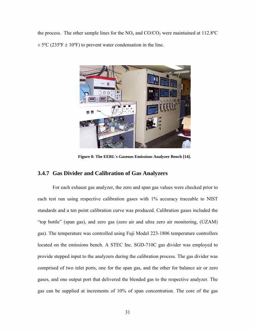
the process. The other sample lines for the NOx and CO/CO2 were maintained at 112.8ºC

± 5ºC (235ºF ± 10ºF) to prevent water condensation in the line.

Figure 8: The EERL's Gaseous Emissions Analyzer Bench [14].

3.4.7 Gas Divider and Calibration of Gas Analyzers

For each exhaust gas analyzer, the zero and span gas values were checked prior to

each test run using respective calibration gases with 1% accuracy traceable to NIST

standards and a ten point calibration curve was produced. Calibration gases included the

“top bottle” (span gas), and zero gas (zero air and ultra zero air monitoring, (UZAM)

gas). The temperature was controlled using Fuji Model 223-1806 temperature controllers

located on the emissions bench. A STEC Inc. SGD-710C gas divider was employed to

provide stepped input to the analyzers during the calibration process. The gas divider was

comprised of two inlet ports, one for the span gas, and the other for balance air or zero

gases, and one output port that delivered the blended gas to the respective analyzer. The

gas can be supplied at increments of 10% of span concentration. The core of the gas

31

divider consists of a set of ten capillaries, and the mass flow rate through each capillary

was proportional to the pressure drop across the capillaries.

3.4.8 Exhaust Gas Analyzers

The exhaust gas analysis bench consisted of laboratory grade (certification

quality) analyzers for measurement of COB2B, CO, NOBxB , and THC. Given below is a

description of each gas analyzer, which is used in the EERL gaseous emissions analyzer

bench.

3.4.8.1 Nitrogen Oxide Analyzer [Rosemount, 1992]

The NO/NOx analyzer used was a Rosemount Model 955 Chemiluminescent

analyzer. This analyzer was capable of detecting concentrations of NO or NO and NO2

together, which also known as NOx. In the NO mode, the analyzer quantitatively

converts NO in the sample into NO2 by gas-phase oxidation with molecular ozone (O3).

Ozone for this reaction is produced by passing air or oxygen over an ultra violet source.

During the oxidation process, approximately 10% of the NO2 molecules are electrically

excited, followed by an immediate return to the non-excited state. This conversion

process generates a photon emission. Then a photomultiplier tube was used to identify the

photon emission quantity, which is proportional to the NO amount present in the sample.

The internal NOx converter was maintained between 660 °F (350 °C) and 750 °F (399

°C) en route for maximum NO2 conversion efficiency. If the determination of NO

concentration only is desired, the sample could bypass the converter and be measured

directly by selecting the NO mode of the analyzer. In the case of NOx detection, the total

analyzer response would determine the amount of NO present in the original sample, as

well as the NO created through the dissociation of NO2 in the converter.

32

3.4.8.2 Hydrocarbon Analyzer [Rosemount, 1992]

A Rosemount Model 402 Heated Flame Ionization Detector (HFID) analyzer was

utilized to measure the Total Hydrocarbon Content (THC) in the diesel exhaust . By

counting the elemental carbon atoms in the exhaust sample the analyzer determined the

amount of hydrocarbon in the exhaust stream. The sample gas flow was synchronized

and flowed through a hydrogen/helium-fueled flame that caused the production of ions.

Ions are produced when a regulated flow of sample gas flows through the flame and are

collected on the polarized electrodes causing current to flow through the associated

electronic measuring circuitry. This assimilation of ions by the electrodes produces a

small current flow, which is then quantified and related to the number of carbon atoms

contained in the exhaust sample. Hydrocarbons are measured wet, which means, water

vapor is not evaporated out from the sample going into the HC analyzer. The multiplier

switch, which is located on the front of the Model 402, allows selection of measurement

ranges which best suits the resolution for the particular gas concentration being sampled.

On the largest scale of the measurement range of the HC analyzer goes up to 250,000

ppm.

3.4.8.3 Carbon Monoxide/Carbon Dioxide Analyzers [Horiba, 2001]

The gaseous constituents of CO and CO2 were determined with Horiba Model

AIA–210LE and Horiba Model AIA-210 Non-Dispersive Infrared (NDIR) analyzers. An

NDIR analyzer operates utilizing the principle of infrared light absorption. NDIR

analyzers use the exhaust gas species being measured to detect itself by the principle of

selective absorption, in which the infrared energy of a particular wavelength, specific to a

certain gas, will be absorbed by that gas. Infrared energy of other wavelengths will be

33

transmitted by that gas, just as the absorbed wavelength will be transmitted by other

gases. This sort of NDIR analyzer does not create a linear output, so calibration curves

were generated for the analyzers before each testing session began.

3.4.9 Fuel Metering System

The fuel metering system was critical, in order to create accurate exhaust

dilution ratios. The total tunnel flow rates were determined with the CFV-CVS system,

but the predicament lies in the understanding of raw exhaust mass flow rates. A few

factors restrain measuring the exhaust flow rate directly, such as engine backpressure

limits, elevated temperatures, and high particulate matter concentrations. So, a different

approach was used to estimate exhaust mass flow rate by understanding intake airflow

rate along with engine fuel consumption rate.

The fuel flow rate was measured with a Max Flow Media 710 Series Fuel

Measurement System [Carder, 1999]. The fuel was drawn from the storage tank exterior

to the lab through a filter and into a vapor removal device, so it could be maintained at

constant pressure of 206.8 kPa (30 psi). Then fuel went through a bypass system where

surplus fuel was routed through a pressure regulator to a heat exchanger and back to the

storage tank. In this process, the heat exchanger used the bypass supply fuel to cool the

engine return fuel. The amount of fuel that was not returned to the tank entered a Model

214 piston-displacement flowmeter and to a level-controlled tank. Within this tank the

metered fuel mixed with the unused engine return fuel which was already cooled by the

internal heat exchanger. The tank maintains its volume constant to measure the fuel used

by the engine. A secondary fuel pump boosted the fuel pressure to the level needed by

high-pressure diesel injection systems such as the common rail system. A bubble

34

detector purged any vapors in the system by controlling a solenoid valve that connected

to-engine and from-engine fuel lines. After departing the solenoid valve, the fuel entered

an external heat exchanger that maintained a constant fuel temperature.

3.4.10 Instrumentation Control/Data Acquisition

Most of the in-laboratory data obtained during the testing undertaken in this study

was collected with software and hardware previously developed and installed at EERL,

other than the software and hardware purchased from National Instruments for cylinder

pressure data acquisition. The in-house data acquisition system used an RTI-815F data

acquisition board for data collection as well as rack-mounted signal conditioning units

(Analog Devices Model 3B). The software and hardware purchased from National

Instruments was discussed above in this chapter. All the laboratory data was recorded in

ADC codes and later converted to the proper engineering units with a Visual Basic based

reduction program developed in-house at WVU EERL.

35

Figure 9: Schematic of West Virginia University’s Engine and Emissions Research Laboratory Emissions Measurement System [14].

36

4 EXPERIMENTAL PROCEDURES

Described below are the procedures and calculations used with in both in-use and

test cell testing phases. These procedures were followed to maintain the accuracy and

distinctiveness of these experiments. Information gathered from Cummins certified

technicians was also mentioned in an attempt to provide some insight on useful life of a

Cummins ISM engines.

4.1 In-Field Data Collection

Since this project was concentrated on Cummins ISM post 2002 engines,

recruitment of on-road vehicles for logging duty cycle data was a challenge. The test

vehicles procured for this project were typically used for mass transportation, commercial

transportation and vocational activities; hence employed on, virtually, a daily basis.

Measures had to be taken to limit downtime and minimize the impact on daily routines.

For instance, the Somat® data logger was installed in all the test vehicles an hour before

the specific vehicle begins its daily schedule. This facilitated the infield data logging with

no additional downtime for the vehicle, thereby limiting the compensation to the owner

that would have been required to pay for the additional time.

4.2 Generation of Micro-Cycles

A diversified collection of data was gathered from four vehicles (heavy hauler,

concrete mixer, transit bus, and dump truck), while they followed operational cycles that

were typical of those encountered in a regular day’s operation. The collection of data

was primarily focused on engine speed and load. After analyzing the whole duty cycle,

37

proportional mini duty cycles were created to capture similar speeds and loads on the

engine. Mini cycles had a duration anywhere from 20 minutes to 45 minutes. The

representative cycles had to be limited to 45 minutes since the limitation of the test cell

data acquisition system. The representative cycles developed from in-field testing were

later recreated in the laboratory using a ISM engine instrumented with a cylinder pressure

transducer, laboratory-grade analyzers and a dynamometer test bed. Before the begin of

test cell testing, speed and load settings applied to the dynamometer were adjusted until

the in-laboratory load and speed data closely correlated with load and speed data taken in

field.

4.2.1 Things Considered During Transient Cycle Generation

The objective of producing a representative transient duty cycle was to include all

the typical, repeatable activities undergone by a vehicle and to record their corresponding

speed-load data in real-time operation. Under transient operation, it is complicated to

optimize the engine parameters. Particulates may be formed due to excess fuel injected

into the cylinder during speed and load changes and a whole host of engine parameters

ranging from turbocharger, in-cylinder temperatures, injection timing, cooled EGR

parameters to exhaust system dynamics and after-treatment systems. Consequently when

developing cycles, the following criteria was observed.

1. The cycle should be representative of similar applications.

2. The developed cycle must involve all in-field operations of the vehicle.

3. The test cycle should go through the maximum range of speed and torque points

in relation to in-field activity.

4. Lengthy idling times should be discarded.

38

5. The cycle should be able to account for the entire accessory load on the original

vehicle.

6. Data should be collected with the same operator during all the in-field trips for a

certain duty cycle.

4.3 Engine Set Up and Break-In

Once the engine arrived in the laboratory, it was set up on a test bed, using engine

mounts as supports. Afterwards, to ensure oil requirements do not affect the emission

measurements, an 80-hour break-in was performed. Any unknown prior damage to the

engine was fixed during the break-in period and so as not to hinder testing afterwards. An

AC dynamometer was used for the break in process and operated the engine at 50%-75%

of the rated load conditions.

For the laboratory testing, a GE® Dynamometer was attached to the engine

flywheel using a driveshaft, an adapter plate, and a bonded-rubber coupling damper made

by Walken®. A new adapter plate was machined to accommodate the fly-wheel bolt

pattern that was unique for this engine. The damper dissipates harmonic vibrations as

well as provides for the absorption of any shock loads that may be encountered during

testing. This drive system has substantial rotational inertia and turns with the same

angular velocity as the engine.

During the testing, charge air cooling was done with water-to-air cooling relative

to air-to-air cooling done in the on-road application. Similarly, engine coolant was

cooled with a water-to-water cross flow heat exchanger relative to the air-to-water

radiator in the field application. Other necessary instrumentations were instrumented to

39

acquire necessary parameters such as EGR inlet/outlet coolant temperature and exhaust

delta pressure.

Additionally, care was taken to keep the retrofit exhaust temperatures and back

pressure values within the CFR specifications for test cell testing. During the testing

backpressure was maintained at 40 (in. of H2O) and the intake restriction was maintained

at 15 (in. of H2O). The exhaust was routed to the primary dilution tunnel by means of

exhaust piping. Joints in the exhaust transfer tube were sealed with aluminum wrap

capable of withstanding the high temperatures. More than 12 ft. (6.1m) of accessible

transfer tube was insulated with exhaust insulation, which was made of fiber-glass wool

and wire mesh. The piping length was insulated in accordance with the requirements of

CFR 40, Part 86. The exhaust transfer tube was insulated to minimize thermophoretic

losses of PM, and to avoid temperatures from falling below 375 °C, which is essential to

avoid condensation of higher molecular weight hydrocarbons. Temperatures were

recorded using J-type thermocouples.

Prior to beginning performance and emissions testing of the engine for its various

duty cycles, the engine was mapped several times to assure the rated conditions and

repeatability. An engine map is a full-load curve for the entire speed domain ranging

from low-idle (700 RPM) through rated speed (2100 RPM) to high idle (2300 RPM).

4.4 Test Matrix

Shown below in Table 7 is the test matrix utilized during the testing. Each duty

cycle was comprised of four micro cycles that was 30-40 minutes in length. Each and

every micro cycle was tested three times to assure repeatability. For the entire testing

intake air was conditioned at 70 C and 50% humidity according to CFR regulations.

40

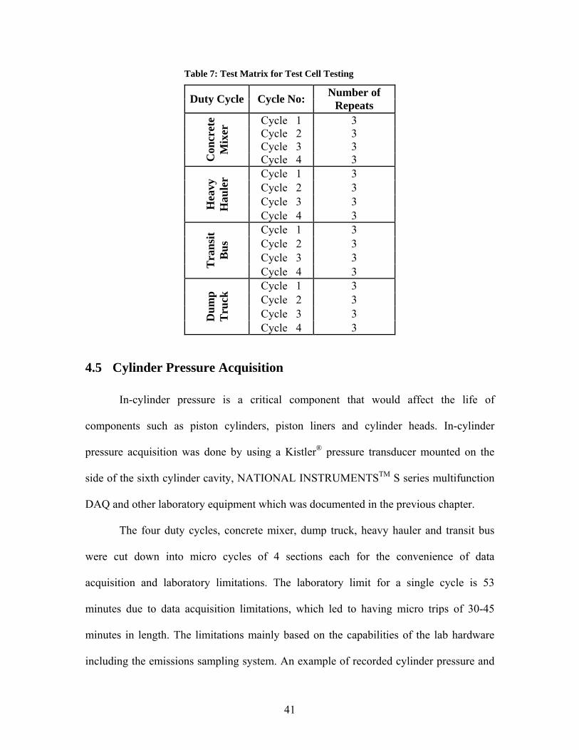
Table 7: Test Matrix for Test Cell Testing

Duty Cycle Cycle No: Number of Repeats

Cycle 1 3 Cycle 2 3 Cycle 3 3

Con

cret

e M

ixer

Cycle 4 3 Cycle 1 3 Cycle 2 3 Cycle 3 3 H

eavy

H

aule

r Cycle 4 3 Cycle 1 3 Cycle 2 3 Cycle 3 3 T

rans

it B

us

Cycle 4 3 Cycle 1 3 Cycle 2 3 Cycle 3 3 D

ump

Tru

ck

Cycle 4 3

4.5 Cylinder Pressure Acquisition

In-cylinder pressure is a critical component that would affect the life of

components such as piston cylinders, piston liners and cylinder heads. In-cylinder

pressure acquisition was done by using a Kistler® pressure transducer mounted on the

side of the sixth cylinder cavity, NATIONAL INSTRUMENTSTM S series multifunction

DAQ and other laboratory equipment which was documented in the previous chapter.

The four duty cycles, concrete mixer, dump truck, heavy hauler and transit bus

were cut down into micro cycles of 4 sections each for the convenience of data

acquisition and laboratory limitations. The laboratory limit for a single cycle is 53

minutes due to data acquisition limitations, which led to having micro trips of 30-45

minutes in length. The limitations mainly based on the capabilities of the lab hardware

including the emissions sampling system. An example of recorded cylinder pressure and

41

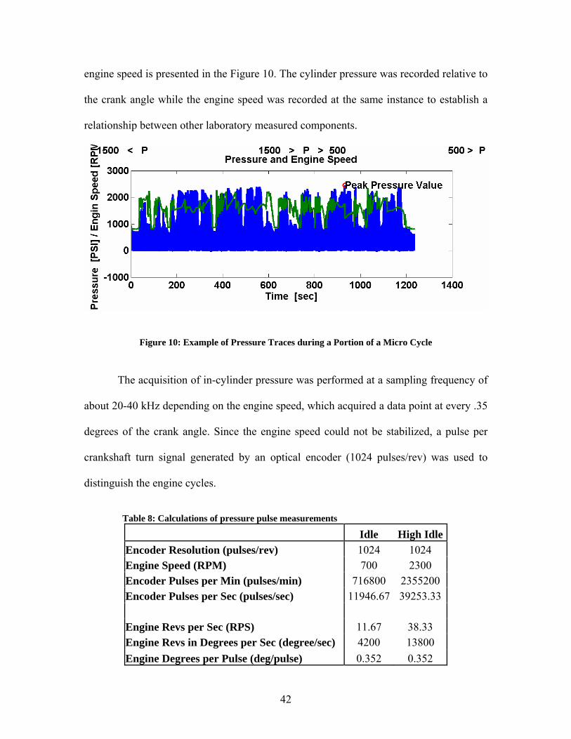
engine speed is presented in the Figure 10. The cylinder pressure was recorded relative to

the crank angle while the engine speed was recorded at the same instance to establish a

relationship between other laboratory measured components.

Figure 10: Example of Pressure Traces during a Portion of a Micro Cycle

The acquisition of in-cylinder pressure was performed at a sampling frequency of

about 20-40 kHz depending on the engine speed, which acquired a data point at every .35

degrees of the crank angle. Since the engine speed could not be stabilized, a pulse per

crankshaft turn signal generated by an optical encoder (1024 pulses/rev) was used to

distinguish the engine cycles.

Table 8: Calculations of pressure pulse measurements

Idle High Idle Encoder Resolution (pulses/rev) 1024 1024 Engine Speed (RPM) 700 2300 Encoder Pulses per Min (pulses/min) 716800 2355200 Encoder Pulses per Sec (pulses/sec) 11946.67 39253.33 Engine Revs per Sec (RPS) 11.67 38.33 Engine Revs in Degrees per Sec (degree/sec) 4200 13800 Engine Degrees per Pulse (deg/pulse) 0.352 0.352

42

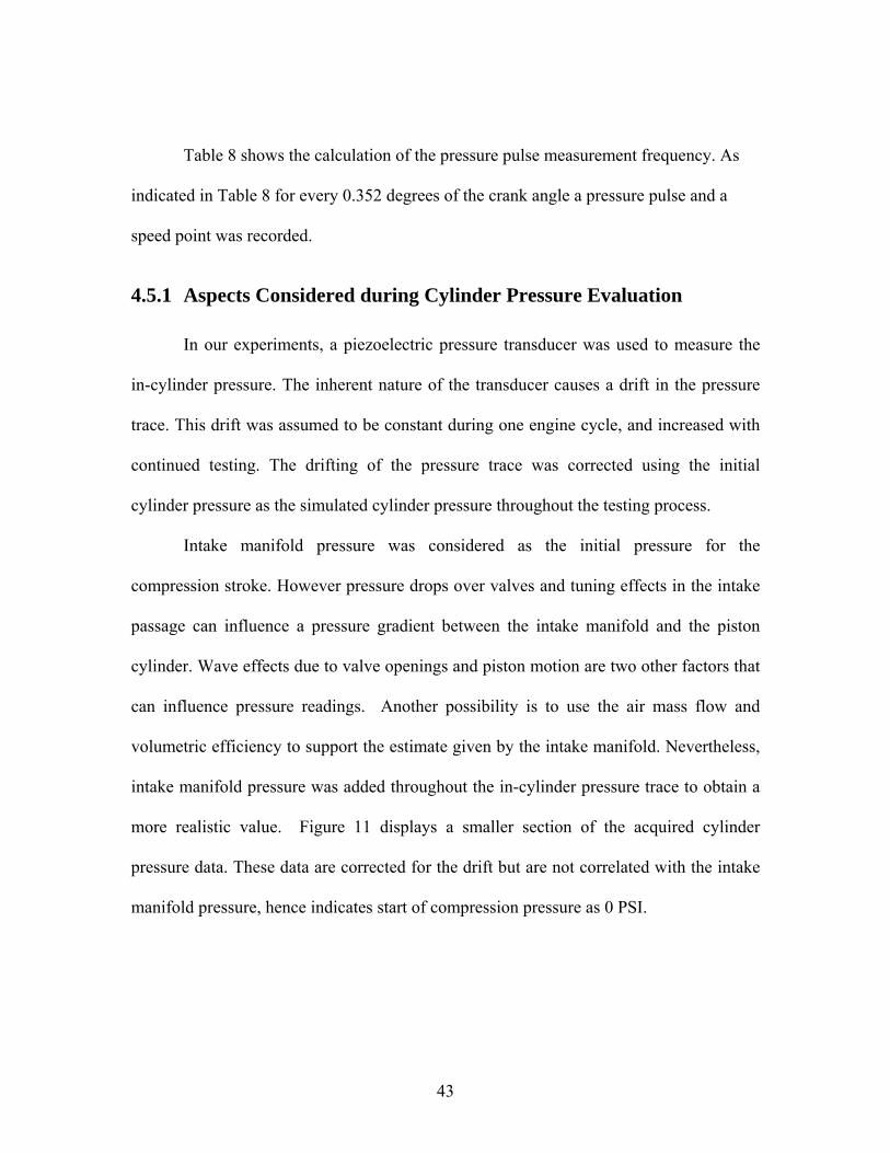
Table 8 shows the calculation of the pressure pulse measurement frequency. As

indicated in Table 8 for every 0.352 degrees of the crank angle a pressure pulse and a

speed point was recorded.

4.5.1 Aspects Considered during Cylinder Pressure Evaluation

In our experiments, a piezoelectric pressure transducer was used to measure the

in-cylinder pressure. The inherent nature of the transducer causes a drift in the pressure

trace. This drift was assumed to be constant during one engine cycle, and increased with

continued testing. The drifting of the pressure trace was corrected using the initial

cylinder pressure as the simulated cylinder pressure throughout the testing process.

Intake manifold pressure was considered as the initial pressure for the

compression stroke. However pressure drops over valves and tuning effects in the intake

passage can influence a pressure gradient between the intake manifold and the piston

cylinder. Wave effects due to valve openings and piston motion are two other factors that

can influence pressure readings. Another possibility is to use the air mass flow and

volumetric efficiency to support the estimate given by the intake manifold. Nevertheless,

intake manifold pressure was added throughout the in-cylinder pressure trace to obtain a

more realistic value. Figure 11 displays a smaller section of the acquired cylinder

pressure data. These data are corrected for the drift but are not correlated with the intake

manifold pressure, hence indicates start of compression pressure as 0 PSI.

43

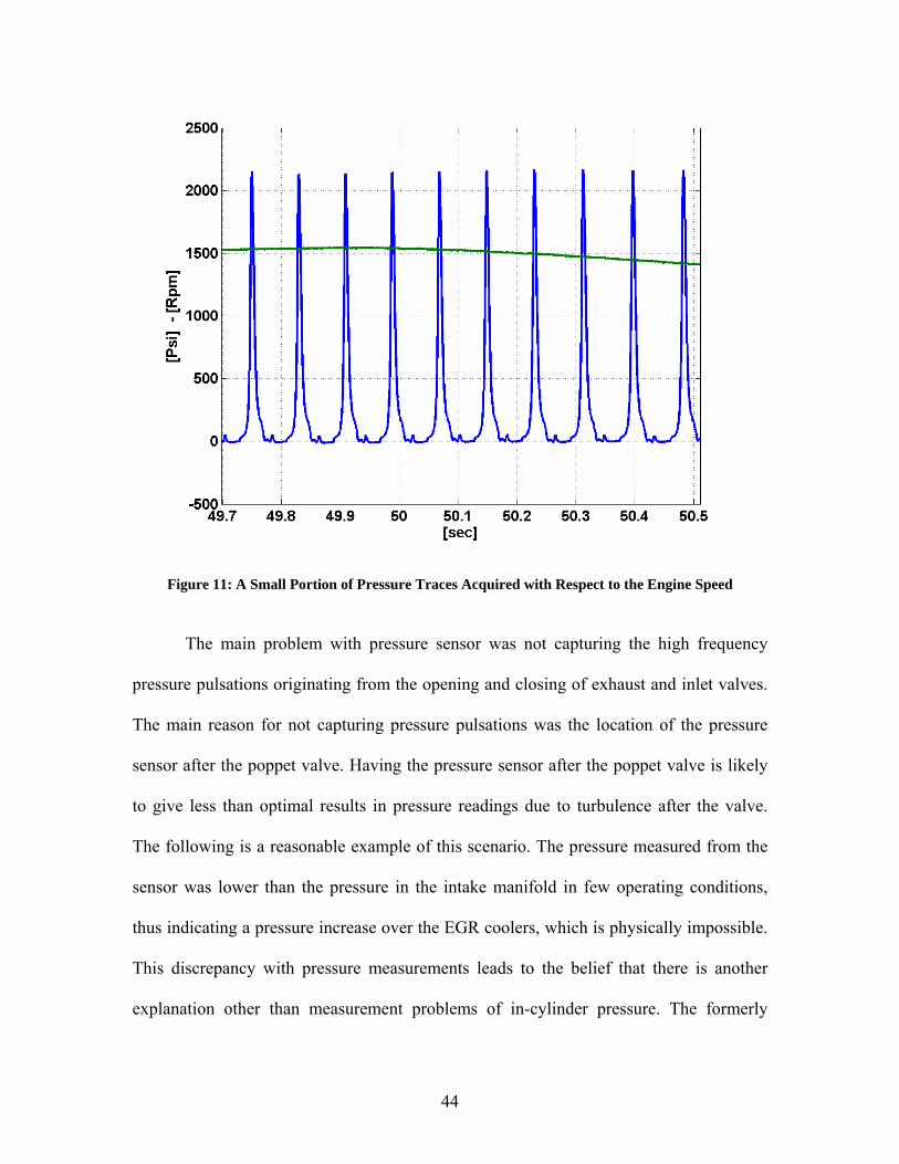
Figure 11: A Small Portion of Pressure Traces Acquired with Respect to the Engine Speed

The main problem with pressure sensor was not capturing the high frequency

pressure pulsations originating from the opening and closing of exhaust and inlet valves.

The main reason for not capturing pressure pulsations was the location of the pressure

sensor after the poppet valve. Having the pressure sensor after the poppet valve is likely

to give less than optimal results in pressure readings due to turbulence after the valve.

The following is a reasonable example of this scenario. The pressure measured from the

sensor was lower than the pressure in the intake manifold in few operating conditions,

thus indicating a pressure increase over the EGR coolers, which is physically impossible.

This discrepancy with pressure measurements leads to the belief that there is another

explanation other than measurement problems of in-cylinder pressure. The formerly

44

discussed pressure pulsations could be one such clarification, where it will drive a flow

through the EGR-system even if the static pressures indicate a flow in the opposite

direction.

4.5.2 Derivation the Volume of Slider-Crank Model

Understanding piston cylinder volume was critical for the calculations of cylinder

pressure. To derive the volume off of a piston cylinder, crank angle is used as a function

of compression ratio, the stroke, bore and connecting rod length (CSU, 2005). These

geometric parameters are identif

ied in the Figure 12.

Figure 12: Piston Cylinder Geometry [3].

b = bore

s = stroke

l = connecting rod length

a = crank radius (= ½ s)

θ = crank angle

TDC = top dead center

BDC = bottom dead center

45

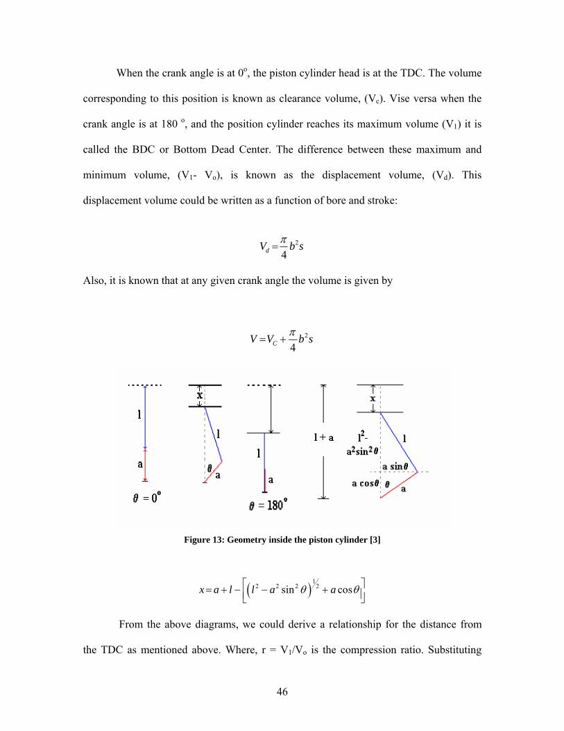
When the crank angle is at 0o, the piston cylinder head is at the TDC. The volume

corresponding to this position is known as clearance volume, (Vc). Vise versa when the

crank angle is at 180 o, and the position cylinder reaches its maximum volume (V1) it is

called the BDC or Bottom Dead Center. The difference between these maximum and

minimum volume, (V1- Vo), is known as the displacement volume, (Vd). This

displacement volume could be written as a function of bore and stroke:

2

4dV b sπ=

Also, it is known that at any given crank angle the volume is given by

2

4CV V b sπ= +

Figure 13: Geometry inside the piston cylinder [3]

( )1

2 2 2 2sin cosx a l l a aθ θ⎡ ⎤= + − − +⎢ ⎥⎣ ⎦

From the above diagrams, we could derive a relationship for the distance from

the TDC as mentioned above. Where, r = V1/Vo is the compression ratio. Substituting

46

known volumes obtained, a final formula was derived for the volume with respect to the

crank angle.

VC = V0 = Minimum Volume

V1 = Maximum Volume

Vd = Displacement Volume

( )

( )

1 1

1

12 2

2

1

1

1 11 cos sin1

d c d c

d c d

c c c

dc

d

V V V V V VV V VVr

V V VVVr

VVr a a

θ θ

= − = +

+= = = +

=−

⎡ ⎤⎛ ⎞⎛ ⎞⎢ ⎥= + + − − −⎜ ⎟⎜ ⎟⎜ ⎟⎢ ⎥− ⎝ ⎠⎝ ⎠⎢ ⎥⎣ ⎦

4.5.3 Work Done by a Piston Cylinder

Figure 14: Work done on the piston due to pressure P [3]

47

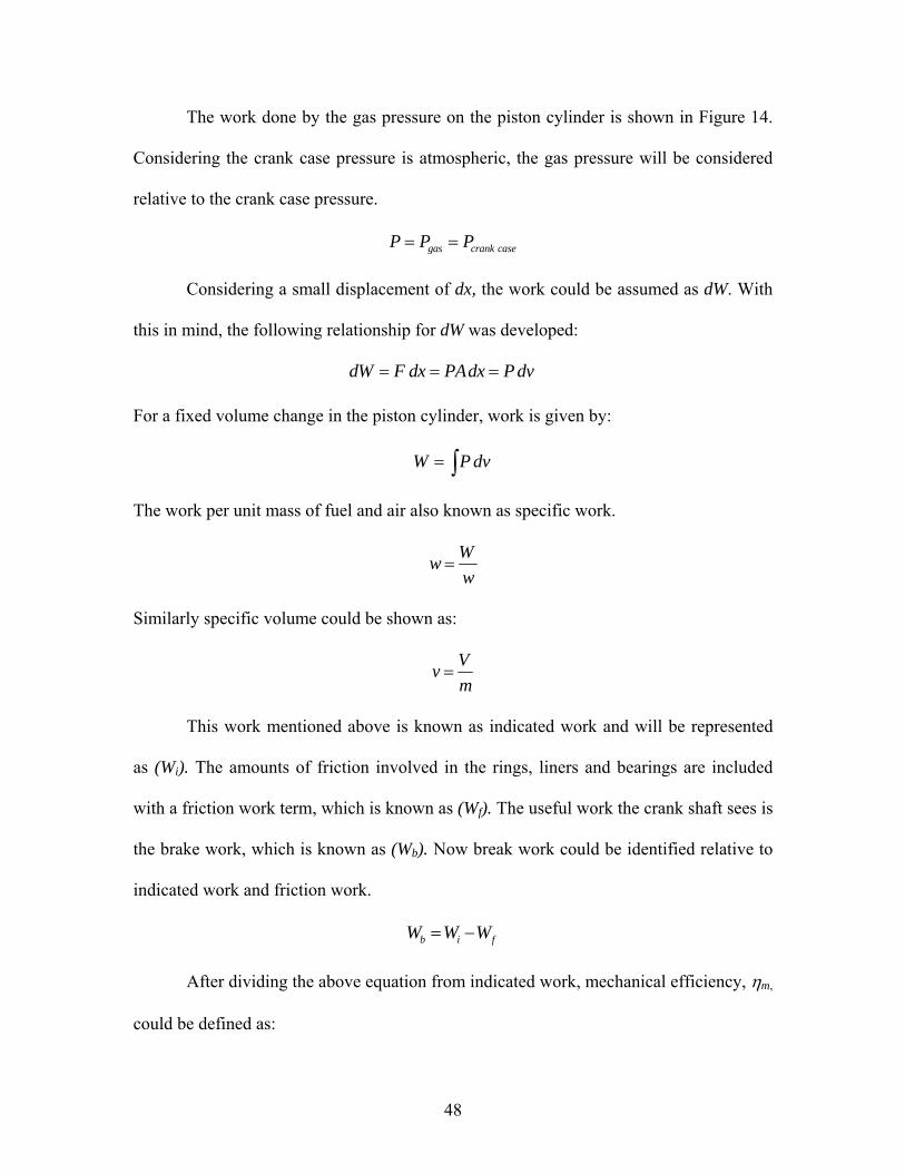
The work done by the gas pressure on the piston cylinder is shown in Figure 14.

Considering the crank case pressure is atmospheric, the gas pressure will be considered

relative to the crank case pressure.

gas crank caseP P P= =

Considering a small displacement of dx, the work could be assumed as dW. With

this in mind, the following relationship for dW was developed:

dW F dx PAdx P dv= = = For a fixed volume change in the piston cylinder, work is given by:

W P d= v∫

The work per unit mass of fuel and air also known as specific work.

Www

=

Similarly specific volume could be shown as:

Vvm

=

This work mentioned above is known as indicated work and will be represented

as (Wi). The amounts of friction involved in the rings, liners and bearings are included

with a friction work term, which is known as (Wf). The useful work the crank shaft sees is

the brake work, which is known as (Wb). Now break work could be identified relative to

indicated work and friction work.

b iW W Wf= −

After dividing the above equation from indicated work, mechanical efficiency, ηm,

could be defined as:

48

1 fbm

i i

WWW W

η = = −

4.5.4 Indicated Mean Effective Pressure

The pressure within a piston cylinder changes regularly with during the expansion

or the power stroke. The pressure increases due to the heat addition, and then decreases

due to the increase in cylinder volume. So, IMEP is used to describe the ideal average

pressure which the engine can output. During the calculation of IMEP, friction of

bearings losses are considered, but the pumping losses of the crankcase are not taken into

account. Now BMEP or brake mean effective pressure can be calculated from the

externally measured torque and, BMEP could be shown in relationship with IMEP as

BMEP IMEP FMEP PMEP= − −

Here FMEP is the friction mean effective pressure (pressure times swept volume

which gives the required work per cycle used for friction) and PMEP is the pumping

mean effective pressure (pressure times swept volume which gives the required work per

cycle used for pumping). BMEP is useful in understanding the engine performance and

state of tune, although, engine rpm should be considered at which the engine is operating

to determine the power potential. Different engines can be compared directly as swept

volume has been removed from the power or torque figures to calculate BMEP, which is

a useful tool in engine performance studies.

Shown below are a few ways of calculating BMEP:

49

2

PowerBMEPSwept Volume RPS

TorqueBMEPSwept Volume

π

=×

× ×=

4.6 ISM Overhauling Information

The overhauling information was obtained from Cummins authorized service

centers, and based upon a majority of their customer’s failure and warranty information.

The overhauling of a diesel engine mainly depends on the mileage it has accumulated.

For a Cummins ISM engine depending on the application, the overhauling intervals are

as follows;

° Short-haul applications – after 500,000 to 600,000 miles.

° Long-haul applications – after 700,000 to 800,000 miles.

Overhauling presents mainly two options, in-frame overhauling and exchanging

the engine for a rebuilt unit. If the option were to have an in-frame overhauling, the

following components will be replaced.

1. Cylinder liners

2. Power cylinder pistons and connecting rods

3. Piston rings

4. Rod bearings

5. Main bearings

6. Cylinder head

7. Optional replacements - Fuel injectors

- Turbo Charger

- Vibrational damper

50

- Lube oil pump

- Water pump

The option of replacing the turbo charger, vibrational damper, fuel injectors,

water pump and the lube oil pump are given to the customer. If the failure occurred in

either the cam-shaft or the crank-shaft or if there’s any visible failure or fatigue signs in

these components, exchanging the engine for a rebuilt unit is recommended.

Considering the external components of the Cummins ISM engine, EGR valve

and the differential pressure tubes have seen the most failure rates. EGR valve failure

occurs due to the sticking of the poppet valve at a certain position inside the EGR valve.

The differential pressure tubes fail due to constant accumulation of particulate matter in

the internal walls.

51

5 RESULTS & DISCUSSION

5.1 Introduction

The objective of this study was to predict the useful life of critical components for

the Cummins ISM diesel engine. Four vehicles (heavy hauler, concrete mixer, transit bus,

and dump truck) were tested on different routes as mentioned earlier in Chapter 3.

Operational cycles were observed in regular days’ operation. The collection of data was

primarily focused on engine speed and load. After analyzing the whole duty cycle,

proportional mini duty cycles were created to capture similar speeds and loads on the

engine. The representative cycles developed from in-field testing were later recreated in

the laboratory environment using an ISM engine.

During the instrumentation process a pressure transducer was installed in the

intake cavity of the sixth cylinder. After the instrumentation, the cylinder pressure

transducer was calibrated to be in-sync with the crank angle.

5.2 Power Cylinder Piston Life Model

The main purpose of this study was to predict the life span of diesel engine

components according to their operating conditions and the duty cycle. If the diesel

engine is considered as a system composed of multiple components for example, n

components, then the system reliability is a product of the individual reliabilities.

( ) ( ) ( )1 2 ...........System nR R R= × × R . En-route to understanding reliability and the life expectations of a diesel engine, it

was important to understand the life of each critical component. This study was

52

performed to evaluate and predict the life cycle of cylinder pressure related to

components such as power piston cylinders, piston liners and cylinder heads. For this, life

and pressure data of the component were gathered from the manufacturers of the

components for the bench tests that have performed. The data was used to create the

model for analyzing and predicting the life of these components. The methodology for

predicting the life of a component proposed in this chapter could be used to evaluate the

life of other critical components and, finally of the diesel engine as a whole system.

5.2.1 Cylinder Pressure Evaluation The acquired pressure data were stored in binary format due to the demanding

nature and storage capabilities. The methods of data storage are described below.

STEP 1 – A MatLab code was developed to translate these binary data into a text file

with three columns for time, pressure and engine speed. These were the only parameters

acquired during the high speed data acquisition phase. While converting binary data, the

program sums up the pressure data with the gathered intake manifold pressures. Intake

manifold pressure data were acquired from the EERL lab setup.

STEP 2 – Another MatLab code was used to create a histogram of the above mentioned

test file with pressure data into a series of bins ranging from 500psi to 2400psi. The

MatLab codes for processing required data can be found in the appendix. After binning

was completed for the pressure data, all four micro cycles in one duty cycle were

combined to form a single cycle. Combining all four cycles had the advantage of

analyzing a single duty cycle as a whole.

Figure 15 illustrates the combined histograms for cylinder pressures in all four

duty cycles. Even though the distributions look somewhat similar, heavy hauler and the

53

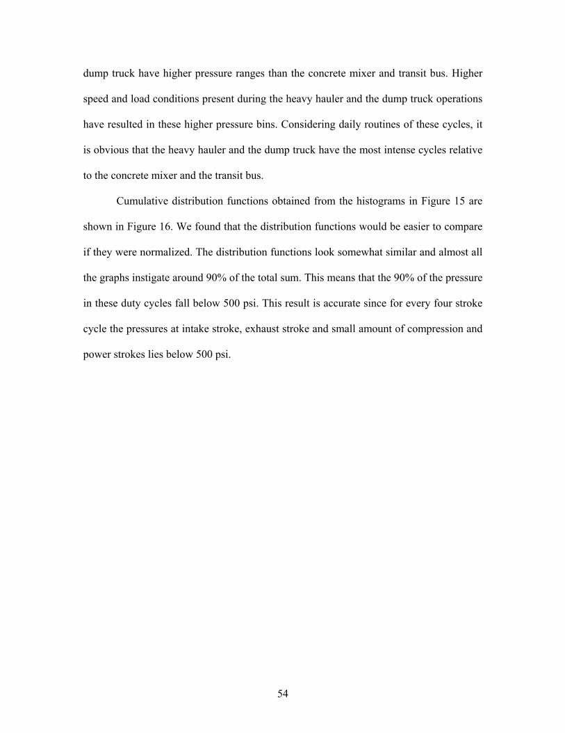
dump truck have higher pressure ranges than the concrete mixer and transit bus. Higher

speed and load conditions present during the heavy hauler and the dump truck operations

have resulted in these higher pressure bins. Considering daily routines of these cycles, it

is obvious that the heavy hauler and the dump truck have the most intense cycles relative

to the concrete mixer and the transit bus.

Cumulative distribution functions obtained from the histograms in Figure 15 are

shown in Figure 16. We found that the distribution functions would be easier to compare

if they were normalized. The distribution functions look somewhat similar and almost all

the graphs instigate around 90% of the total sum. This means that the 90% of the pressure

in these duty cycles fall below 500 psi. This result is accurate since for every four stroke

cycle the pressures at intake stroke, exhaust stroke and small amount of compression and

power strokes lies below 500 psi.

54

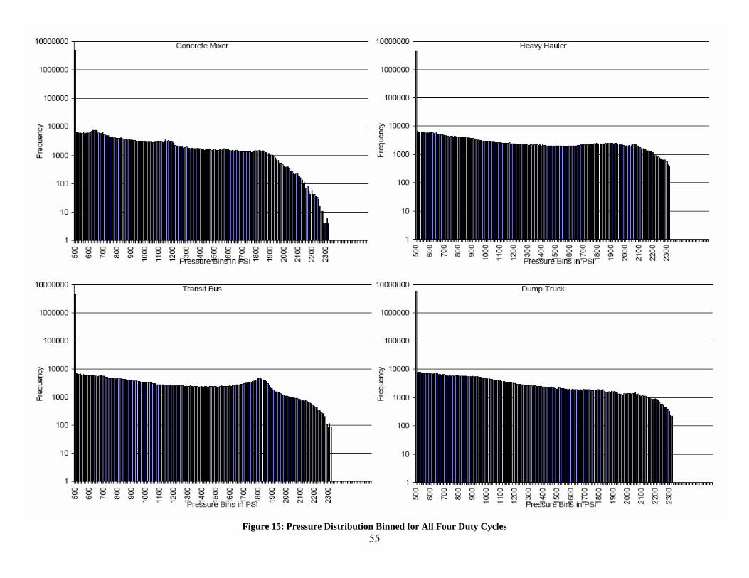
55Figure 15: Pressure Distribution Binned for All Four Duty Cycles

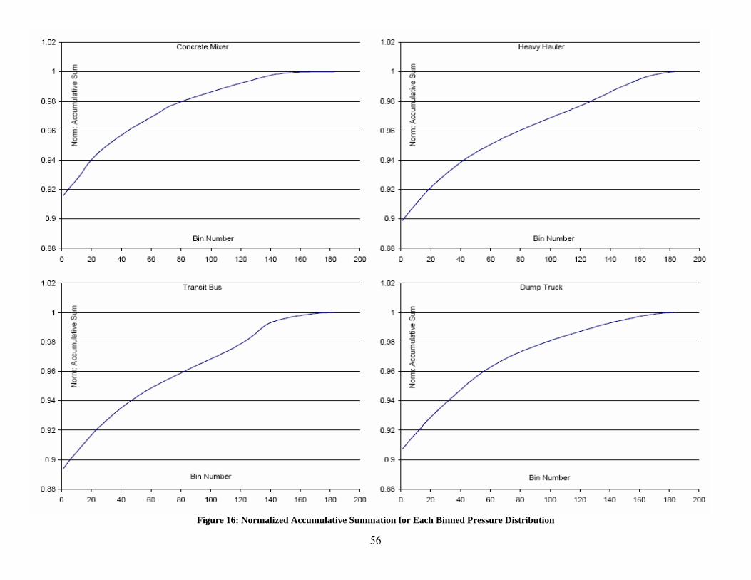
Figure 16: Normalized Accumulative Summation for Each Binned Pressure Distribution

56

5.2.2 Evaluating the Life Estimation Problem Consider two sets of data. The first set includes pressure data for 4 duty cycles.

The other set is composed of four points each representing the average life of power

cylinder pistons for one of the engine duty cycles. The major objective of this section is

to estimate a continuous function that related the pressure data and the “life” points. This

is a non-linear regression problem.

To be more specific, given four sets of data

( )( ) ( )( ) ( )( ) ( )( )(1) (1) (2) (2) (3) (3) (4) (4), , , , , , ,G y G y G y G yi i i i , where ( )( ) ,iG i i=1,…..,4 is

the distribution function of the cycle pressure data for the ith application and y(i), i=1,…,4

is the average life point characterizing the ith application. The life points y(1),…, y(4) are

pre-determined. Ideally, these life data should be obtained from the bench tests that the

component manufactures have performed.

Figure 17 illustrates the forward model: the mapping of input data into the output

data using an unknown function ( )f i . The problem of continuous function estimation

from a finite amount of data (only 4 pairs of input-output data are available) is an ill-

posed problem. In order to regularize the problem, that is, to make it well-posed the

following approach was proposed.

1. We first reduced the dimension of the input data. The entire distribution function

of the pressure data is approximated using a B-spline based approximation with 3

simple B-spline functions. Thus the distribution function, a continuous function,

was now represented by 3 coefficients in the B-spline based approximation.

2. We approximated the mapping function, ( )f i , using linear combination of 2

multidimensional Radial Basis Functions (RBF), that is,

57

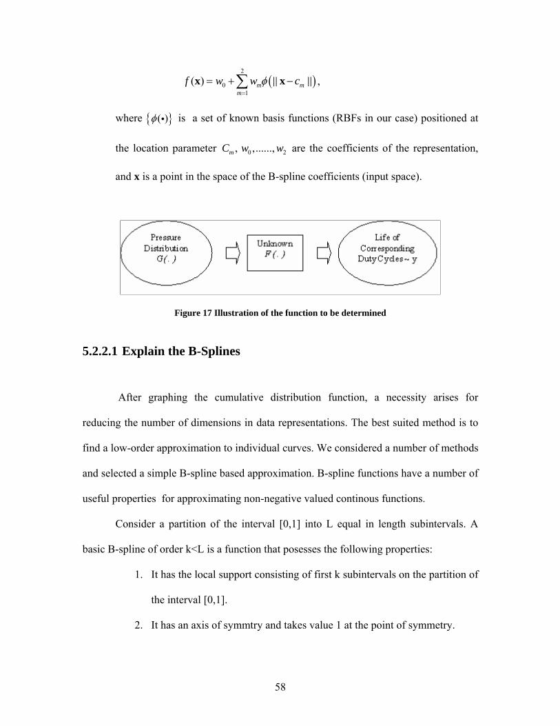
(2

01

( ) mm

f w w cφ=

= + −∑x )mx ,

where { }( )φ i is a set of known basis functions (RBFs in our case) positioned at

the location parameter are the coefficients of the representation,

and x is a point in the space of the B-spline coefficients (input space).

0, ,......,mC w w2

Figure 17 Illustration of the function to be determined

5.2.2.1 Explain the B-Splines

After graphing the cumulative distribution function, a necessity arises for

reducing the number of dimensions in data representations. The best suited method is to

find a low-order approximation to individual curves. We considered a number of methods

and selected a simple B-spline based approximation. B-spline functions have a number of

useful properties for approximating non-negative valued continous functions.

Consider a partition of the interval [0,1] into L equal in length subintervals. A

basic B-spline of order k<L is a function that posesses the following properties:

1. It has the local support consisting of first k subintervals on the partition of

the interval [0,1].

2. It has an axis of symmtry and takes value 1 at the point of symmetry.

58

3. It is (k-1) times continously differentiable at any point within the region

of its support.

4. The B-spline of order k, denote B(k)(t), can be obtained by convolving k

B-splines of order 1, B(1)(t), that is,

( ) (1) (1)( ) ( ) ... ( )k

k fold convolution

B t B t B t

−

= ∗ ∗←⎯⎯⎯⎯⎯⎯→

.

The example of simple B-spline function of order 1,2, and 3 are shown in

Figure 18.

Figure 18: B-spline function of order 1,2, and 3

59

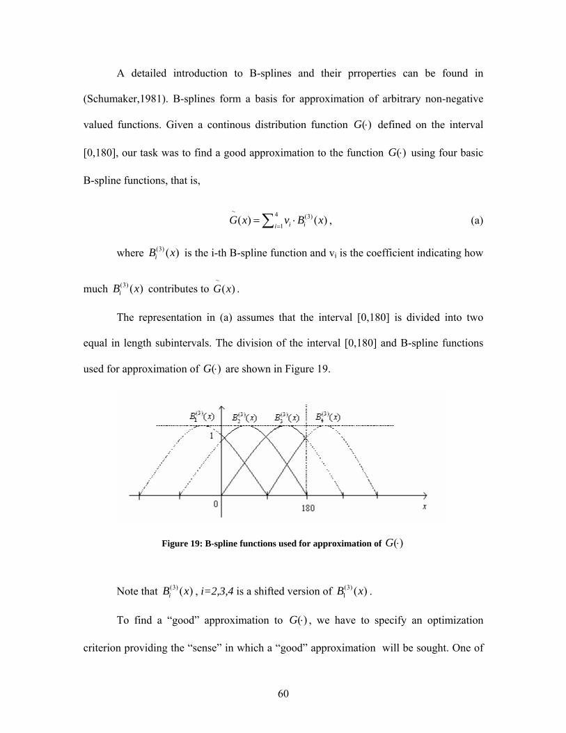
A detailed introduction to B-splines and their prroperties can be found in

(Schumaker,1981). B-splines form a basis for approximation of arbitrary non-negative

valued functions. Given a continous distribution function ( )G ⋅ defined on the interval

[0,180], our task was to find a good approximation to the function using four basic

B-spline functions, that is,

( )G ⋅

, (a) ~ 4 (3)

1( ) ( )i ii

G x v B x=

= ⋅∑

where is the i-th B-spline function and v(3) ( )iB x i is the coefficient indicating how

much contributes to . (3) ( )iB x~

( )G x

The representation in (a) assumes that the interval [0,180] is divided into two

equal in length subintervals. The division of the interval [0,180] and B-spline functions

used for approximation of are shown in Figure 19. ( )G ⋅

Figure 19: B-spline functions used for approximation of ( )G ⋅

Note that , i=2,3,4 is a shifted version of . (3) ( )iB x (3)1 ( )B x

To find a “good” approximation to ( )G ⋅ , we have to specify an optimization

criterion providing the “sense” in which a “good” approximation will be sought. One of

60

the most commonly used criterion in the theory of function approximations is the

integrated least square criterion given by

2180 4

10

min( ) ( )

, 1,...4 k kki

G x v B x dxv i =

− ⋅= ∑∫ . (b)

Note that the function approximation problem is reduced to the problem of

finding v1,…,v4 that solve (b). We used the functions spap2() and fnval() from the spline

toolbox in matlab to solve (b) for v1,…,v4. The results are presented and discussed in

section 5.2.3.

5.2.2.2 Understanding Radial Basis Functions

Understanding the life of certain engine components requires nonlinear mapping

of points in a multi dimensional input space onto the real life (output space). RBFs are a

set of functions that are often used to approximate the unknown nonlinear mapping

function.

The major benefit of using RBFs is the considerable amount of flexibility in

adopting shape and location parameters.

A multidimensional mapping ( )f x can be approximated using a vector based RBF as

( )~

01

( )CN

m mm

f x W W x Cφ=

= + −∑ ,

where ~

( )f x is an approximation to ( )f x , while are the

coefficients of the approximation and

0 ,........,CNw w

, 1,.....,mC m NC= are location parameters.

In a network or a similar system, that is connected with RBFs the input is linked

to the RBF via a center component (c) while the RBF is linked to the output through a

weight component (w). Since the functions that need to be estimated are scalar, a

61

relationship could be established between input ( )x µ and output ( )f µ , using the previous

equation

( )( ) ( )0

1

CN

m mm

f w w x cµ µφ=

= + −∑ .

Expanding this when µ = 1,……, P

( )(1) (1)0

1

CN

m mm

f w w x cφ=

= + −∑

( )( ) ( )0

1

CNP P

m mm

f w w x cφ=

= + −∑

or using the matrix notation

(1)(1) (1)(1)

01 2(2)(2) (2)(2)

11 2

( ) ( )( ) ( )1 2

11

1

C

C

CC

N

N

P PP PNN

f W

wfwf

wf

φφ φφφ φ

φ φ φΦ

⎛ ⎞⎛ ⎞⎛ ⎞⎜ ⎟⎜ ⎟⎜ ⎟⎜ ⎟⎜ ⎟⎜ ⎟ = ⎜ ⎟⎜ ⎟⎜ ⎟⎜ ⎟⎜ ⎟⎜ ⎟⎜ ⎟ ⎜ ⎟⎜ ⎟⎝ ⎠ ⎝ ⎠⎝ ⎠

,

where ( )( ) ( )i i

j X Cφ φ= − j . The above indicated relationship could be written

as f W=Φ , where Ф is known as the interpolation matrix, while W are the weights in

the approximation ~f to the unknown function f.

Solving for a good approximation requires identifying the types of RBFs,

the centers of RBFs, (c

( )~f x

m), and the weights (wm).

Function selection is an important part in solving RBFs. During this study a

Gaussian type of function was used. A Gaussian function has a local representation and is

given by

62

( )2

2reξ

φ ξ⎛ ⎞−⎜ ⎟⎜⎝=

⎟⎠ , where

r is the parameter that determines the effective domain of the RBFs. The Gaussian

RBF positioned at the center Cm is then

( )( )

2 2( )

12exp

mk k

km

x cx c

rφ =

⎛ ⎞−⎜ ⎟

⎜ ⎟− = −⎜ ⎟⎜ ⎟⎝ ⎠

∑.

A multidimensional Gaussian RBF has a nice property of being factored into a

product of one dimensional Gaussian RBFs

( ) ( )2( )2

21

expm

k km

k

x cx c

rφ

=

⎛ ⎞−⎜ ⎟− = −⎜ ⎟⎝ ⎠

∏ .

5.2.2.3 Implementation of Radial Basis Function

To find a “good” approximation to the unknown function ~

( )f x we induce the

least square criterion:

~2f yℑ = − ,

where ~f is the estimated life and y is the actual life obtained from the manufacturer and

solve the following minimization problem

2~4

1 1 2 1min( , , , ) ij j

r y f x= −

⎡ ⎤⎛ ⎞⎢ ⎥= − ⎜ ⎟⎝ ⎠⎢ ⎥

⎣ ⎦∑w c c (c)

63

Thus, the problem of function estimation ~

( )f x is reduced to estimation of a

number of parameters including and C0 1 2, ,w w w 1,C2, and r.

The global optimization in discrete space can be performed exhaustively in three

steps as described below.

STEP 1 – Choosing r parameterizing the Gaussian Radial Basis Function

( )22( ) exp xg x r= − .

Figure 20: r values were selected in relation to the coefficients of B-splines The values of the r-parameters are selected by examining the coefficients of the

B-splines approximating the pressure distributions. Figure 20 illustrates the influence of

increasing the value of the parameter r on the spread of the B-spline coefficients. The

selection criteria are the spread of the coefficients and the minimum and the maximum

values. After careful investigation, four values were selected for the r vector. For every

single r value, calculations were performed to optimize the final result. The values of r

vector are as follows

{ }0.1,0.2,0.3,0.4∈r .

64

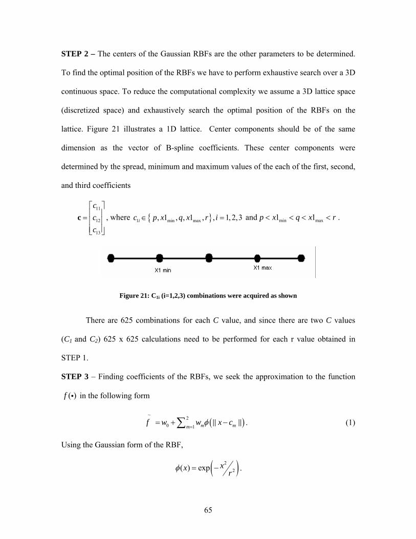
STEP 2 – The centers of the Gaussian RBFs are the other parameters to be determined.

To find the optimal position of the RBFs we have to perform exhaustive search over a 3D

continuous space. To reduce the computational complexity we assume a 3D lattice space

(discretized space) and exhaustively search the optimal position of the RBFs on the

lattice. Figure 21 illustrates a 1D lattice. Center components should be of the same

dimension as the vector of B-spline coefficients. These center components were

determined by the spread, minimum and maximum values of the each of the first, second,

and third coefficients

11

12

13

ccc

⎡ ⎤⎢ ⎥= ⎢ ⎥⎢ ⎥⎣ ⎦

c , where { }1 min max, 1 , , 1 , , 1, 2,3ic p x q x r i∈ = and min max1 1p x q x r< < < < .

Figure 21: C1i (i=1,2,3) combinations were acquired as shown

There are 625 combinations for each C value, and since there are two C values

(C1 and C2) 625 x 625 calculations need to be performed for each r value obtained in

STEP 1.

STEP 3 – Finding coefficients of the RBFs, we seek the approximation to the function

( )f i in the following form

. (1) (~

20 1 mm

f w w x cφ=

= + −∑ )m

Using the Gaussian form of the RBF,

( )22( ) exp xx rφ = − .

65

Thus we have ( )( )2( )

12exp

nm

k kk

m

x cx c

rφ =

⎛ ⎞−⎜ ⎟

⎜ ⎟− = −⎜ ⎟⎜ ⎟⎝ ⎠

∑.

Simplifying further with the multiplicative property of exponent,

( ) ( )2( )

21

expmn

k km

k

x cx c

rφ

=

⎛ ⎞−⎜− = −⎜⎝ ⎠

∏ ⎟⎟

(2)

and substituting (2) into (1),we obtain

( )2( )~2

0 211

expmn

k kmm

k

x cf w w

r==

⎛ ⎞⎛ ⎞−⎜ ⎜= + −⎜ ⎜⎜ ⎟⎝ ⎠⎝ ⎠∑ ∏ ⎟⎟

⎟⎟

)

. (3)

Since there are four input-output pairs ( ) ( )( ,k yµ µx , µ=1,…,4 for the four different duty

cycles, we compose four equations

( )2( ) ( )~

2( )0 21

1

exp , 1,..., 4mn

k kmm

k

x cf w w

r

µµ µ

==

⎛ ⎞⎛ ⎞−⎜ ⎟⎜ ⎟= + − =⎜ ⎟⎜ ⎟⎜ ⎟⎝ ⎠⎝ ⎠∑ ∏ .

Now, consider the objective function,

2~4 ( ) ( )

1J y fµ µ

µ=

⎛ ⎞= −⎜

⎝ ⎠∑ ⎟ (4)

that can be re-written in the vector form as follows

~ ~T

J y f y f⎛ ⎞ ⎛ ⎞= − −⎜ ⎟ ⎜ ⎟⎝ ⎠ ⎝ ⎠

.

Since we know , ~f w

−= Φ ⋅

substituting ~f in (4) ( ) ( )TJ y w y wφ φ= − − .

66

After expanding the above error function we have

T T T TTJ Ty y w y y w w wφ φ φ φ− − − −− − − −

= − − + (5)

where, .

(1) (1)(1)1 2

0(2) (2)(2)1 2

1(3) (3)(3)1 2

2(4) (4)(4)1 2 (3 1)

(4 1) (4 3)

11

, ,11

yw

yy w

yw

y

φ φφ φφ φφ φ

×× ×

⎛ ⎞⎛ ⎞⎛ ⎞⎜ ⎟⎜ ⎟⎜ ⎟⎜ ⎟⎜ ⎟= Φ = =⎜ ⎟⎜ ⎟⎜ ⎟ ⎜ ⎟⎜ ⎟⎜ ⎟ ⎝ ⎠⎜ ⎟ ⎜ ⎟

⎝ ⎠ ⎝ ⎠

w

0

Our goal is to find a set of weights w0,w1, and w2 that minimize the expression in (4).

After differentiating both sides of the equation (5) with respect to and setting the

derivative to zero

w−

( ) T TT Tw J y w y wφ φ φ φ φ

− −− −−∇ = − − = − + =

we obtain the following solution

1( )TT Tw y φ φ φ −

−= .

Thus the optimal set of weights resulting in the optimal approximation to function ( )f i

are given by

* 1( )T Tw yφ φ φ−

− −= . (6)

Together with optimal weights 0

*1

2

www

−

⎡ ⎤⎢ ⎥= ⎢ ⎥⎢ ⎥⎣ ⎦

w we can easily find the corresponding

value of the least square function.

Now, given the estimated weights vector *w−

, coefficient , vectors and

and cylinder pressure data describing a new application, the life of the new application

can be estimated by taking the following steps:

*1r

*

1c *

2c

67

1. Find the distribution function of the cylinder pressure data, describing the

new application.

2. Obtain the best approximation of the distribution function in-terms of B-

splines of the 2nd order. Using 3rd and 4th order B-splines will give us a

better representation on the distribution. Denote B-spline coefficients by

. z−

3. Map the weights of B-splines into the “life” space. To perform this step,

use the estimated function ~f with *w

−, , , and substituted in place

of initially unknown parameters, that is

*r *

1c *

2c

( )( )

2*3

21 *

( )*~ 2* *

0 1( )

ik k

k

z c

rim

f w w e=

⎛ ⎞−⎜ ⎟− ⎜ ⎟⎜⎝

=

∑= + ⋅∑z

⎟⎠ , (7)

where are the coefficients of B-spline approximations obtained using

data for the new application.

z−

5.2.3 Numerical Results For piston cylinders bench test data were modeled in terms of cylinder pressure

and piston cylinder life. The distribution functions obtained from the pressure data

describing cycle 1- cycle 4 are shown in Figure 22. Also, in the same graph the B-spline

based approximations are graphed for the corresponding pressure distribution. The B-

spline coefficients characterizing the distributions of cylinder pressure and the life data

are summarized in Table 9. The lives for the pressure distributions were synthetically

generated considering the roughness and the loads for the individual duty cycle.

68

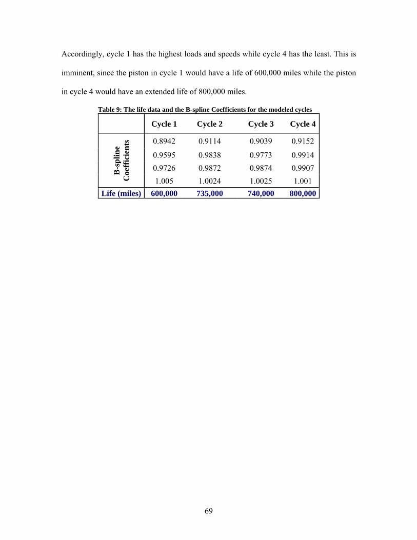
Accordingly, cycle 1 has the highest loads and speeds while cycle 4 has the least. This is

imminent, since the piston in cycle 1 would have a life of 600,000 miles while the piston

in cycle 4 would have an extended life of 800,000 miles.

Table 9: The life data and the B-spline Coefficients for the modeled cycles

Cycle 1 Cycle 2 Cycle 3 Cycle 4

0.8942 0.9114 0.9039 0.9152

0.9595 0.9838 0.9773 0.9914 0.9726 0.9872 0.9874 0.9907 B

-spl

ine

Coe

ffic

ient

s

1.005 1.0024 1.0025 1.001 Life (miles) 600,000 735,000 740,000 800,000

69

70

Figure 22: Shown are Cumulative Distribution Functions for Each Binned Pressure Distribution (Assumed Cycles) Graphed jointly with the Corresponding B-spline Approximations.

As mentioned above in Step 1, four r parameterizing values were selected for the RBFs

that could be used in the calculations of the mapping function ( )f ⋅

{ }0.1,0.2,0.3,0.4∈r .

After solving (c) w.r. to r, we selected r = 0.4. As described in Step 2, it was critical to

find the optimal values for both C1 and C2. There are 625 combinations for each C value, and

since there are two C values (C1 and C2) 625 x 625 calculations need to be performed. Table 10

shows the 25 values that could be selected for both C1 and C2.

Table 10: The possibilities for C1 and C2 CI CII CIII CIV

0.9059 0.9803 0.9957 0.9867 0.9159 0.9903 1.0057 0.9956 0.9259 1.0003 1.0157 0.9768 0.9359 1.0103 1.0257 1.02 0.9459 1.0203 1.0357 1.0356

71

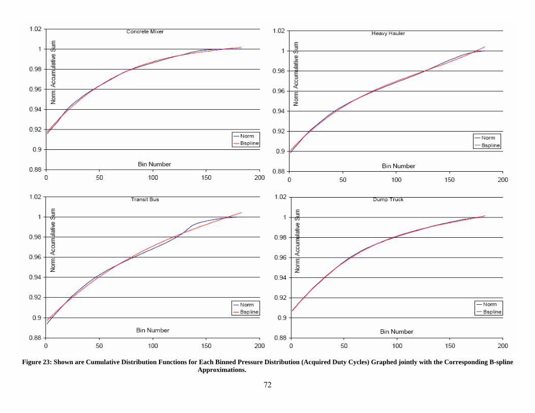
Figure 23: Shown are Cumulative Distribution Functions for Each Binned Pressure Distribution (Acquired Duty Cycles) Graphed jointly with the Corresponding B-spline

Approximations.

72

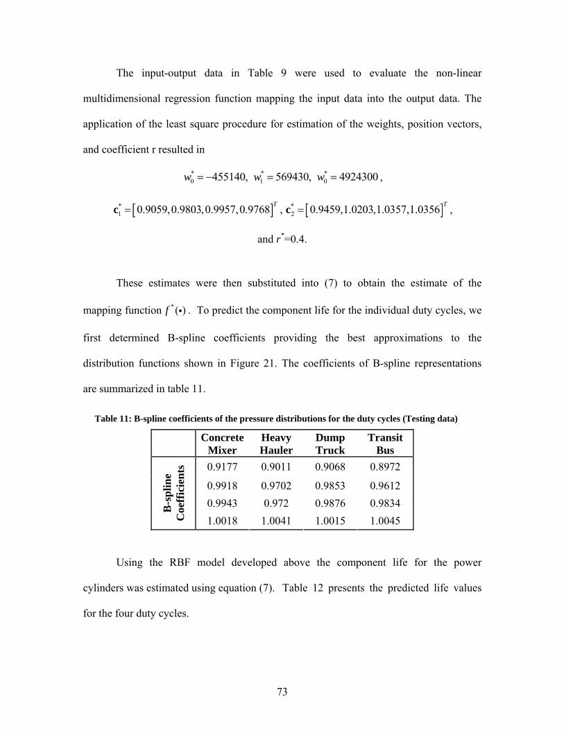
The input-output data in Table 9 were used to evaluate the non-linear

multidimensional regression function mapping the input data into the output data. The

application of the least square procedure for estimation of the weights, position vectors,

and coefficient r resulted in

* * *0 1 0455140, 569430, 4924300w w w= − = = ,

[ ] [ ]* *1 20.9059,0.9803,0.9957,0.9768 , 0.9459,1.0203,1.0357,1.0356T T= =c c ,

and r*=0.4.

These estimates were then substituted into (7) to obtain the estimate of the

mapping function . To predict the component life for the individual duty cycles, we

first determined B-spline coefficients providing the best approximations to the

distribution functions shown in Figure 21. The coefficients of B-spline representations

are summarized in table 11.

*( )f i

Table 11: B-spline coefficients of the pressure distributions for the duty cycles (Testing data)

Concrete Mixer

Heavy Hauler

Dump Truck

Transit Bus

0.9177 0.9011 0.9068 0.8972

0.9918 0.9702 0.9853 0.9612 0.9943 0.972 0.9876 0.9834 B

-spl

ine

Coe

ffic

ient

s

1.0018 1.0041 1.0015 1.0045

Using the RBF model developed above the component life for the power

cylinders was estimated using equation (7). Table 12 presents the predicted life values

for the four duty cycles.

73

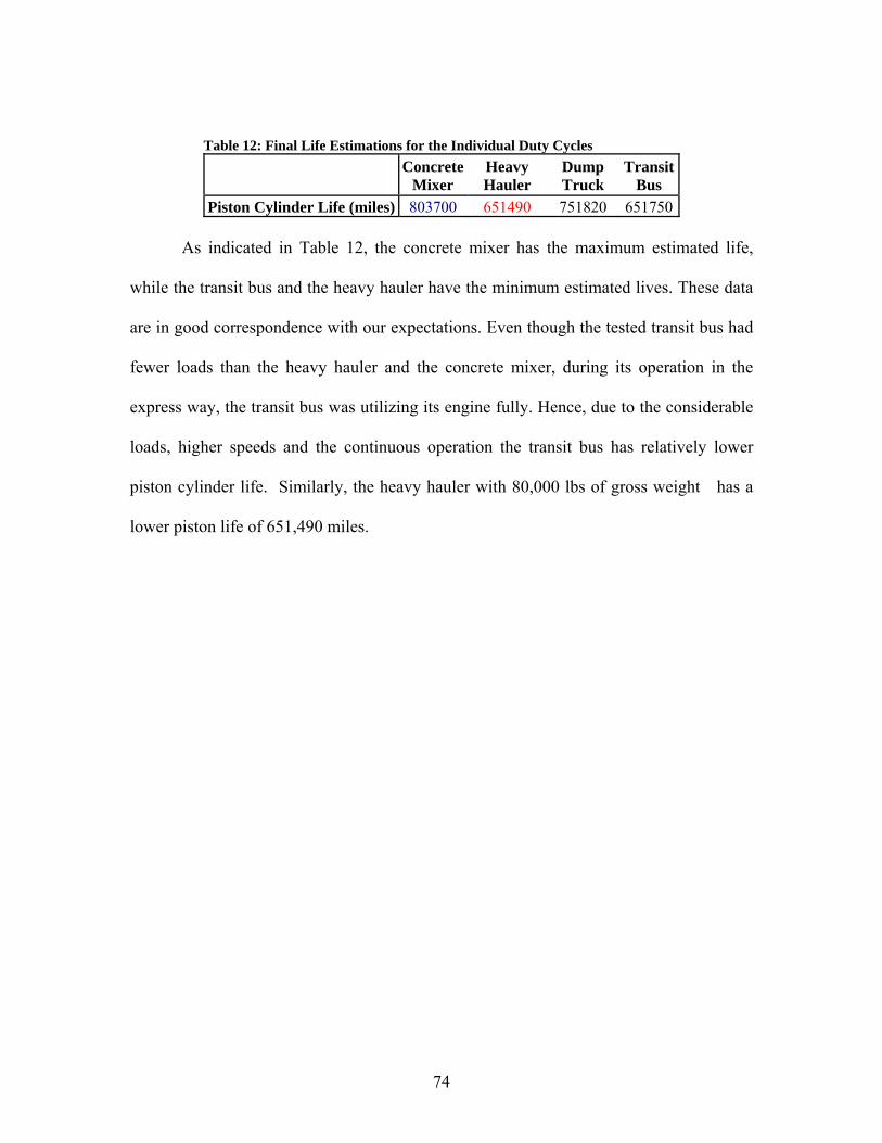
Table 12: Final Life Estimations for the Individual Duty Cycles

Concrete

Mixer Heavy Hauler

Dump Truck

Transit Bus

Piston Cylinder Life (miles) 803700 651490 751820 651750 As indicated in Table 12, the concrete mixer has the maximum estimated life,

while the transit bus and the heavy hauler have the minimum estimated lives. These data

are in good correspondence with our expectations. Even though the tested transit bus had

fewer loads than the heavy hauler and the concrete mixer, during its operation in the

express way, the transit bus was utilizing its engine fully. Hence, due to the considerable

loads, higher speeds and the continuous operation the transit bus has relatively lower

piston cylinder life. Similarly, the heavy hauler with 80,000 lbs of gross weight has a

lower piston life of 651,490 miles.

74

6 CONCLUSIONS & RECOMENDATIONS

6.1 Conclusions The performance testing and cycle development work performed for this study

provides additional information needed for the development of testing protocols for

diesel-powered on-highway equipment. The data produced through this research could

be used to promulgate a better understanding of the various duty-cycles and help develop

requirements for these heavy-duty vehicles.

This study also demonstrates that, even though all vehicles utilize the same engine

with similar ratings, the cylinder loads depend largely on the application. From the

applications discussed, the heavy hauler application has the most detrimental effect on

piston life, while concrete mixer has the least. This is a result of the normal operating

speed and load of the respective engines. The heavy hauler operates twice as fast as the

concrete mixer. These added stresses along with the higher operating load cause the most

rapid decline of piston life. The heavy hauler is rated for operation with a vehicle weight

of 80,000 lb, where the concrete mixer was only rated for 45,000 lb. Though the engine

speed plays a role on component wear, it is shown that in cylinder pressure has the

primary role in determining the component life. It was shown that without affecting the

other parameters, that the in cylinder pressure caused a dramatic reduction of material

life.

The data shows a trend that can be used to predict the loads and subsequent

requirements of engine performance for each respective duty cycle. This will greatly aid

further design and reduce the over design of these engines and components. Production

75

cost should be reduced as less material is required. Vehicle performance will likely be

enhanced from a lighter more efficient engine.

It should be noted that this is an initial study and serves to better inform and direct

the efforts of researchers and designers. Further efforts should include a wider range of

duty cycles. It would be advantageous to have vehicles of the same work rating operate

through a range of duty cycles to better identify the complete impact of each type of duty

cycle. As the duty cycle has a critical role in the component and engine life, the

combined effects of temperature with the duty cycle and in cylinder pressures is not yet

known. This is of concern since these engines must perform in all environments. It is

strongly recommended that an expanded study of temperature, in cylinder pressure, and

more duty cycles be performed.

6.2 Future Work

The work on in-cylinder pressure for various duty cycles can be studied on off-

road vehicles as well. This work also could be performed on other engine families to

establish trends based on the performance of the respective family. From these trends the

engine family will be optimized for performance. Ultimately this research and

development will be expanded to encompass multiple parameters so that the design

models will approach the actual engine. A database could be created with duty cycle

information, in-cylinder pressure data, and component life data. This will allow the

manufacturer to rapidly model or tailor an engine for various customer requirements.

76

7 REFERENCES 1. “Life Data Analysis (Weibull Analysis)”, Weibull.com, 02 Oct 2005, 15 Nov

2005, http://www.weibull.com/basics/lifedata.htm. 2. “Reciprocating Internal Combustion Engines – Exhaust Emissions Measurement”, International Organization for Standardization, ISO/DIS 8178, Geneva, Switzerland, 1993. 3. “Slider Crank Model”, Colorado State University Engineering College, 15 Nov

2005,25 Nov 2005, http://www.engr.colostate.edu/%7Eallan/thermo/page2/page2.html

4. “Accelerated Life Testing Data Analysis ”, Weibull.com, 04 Apr 2005, 15 Nov

2005, http://www.weibull.com/basics/accelerated.htm. 5. Aldridge, D. S., “An Introduction to Generating Vibration Durability Test

Specifications for Automotive Engine Mounted Components”, AC Rochester Division of GMC.

6. Aldridge, D. S., “A General Process for Defining Durability Requirements”,

Delphi-Energy And Chassis Division, 2004. 7. Aldridge, D. S., “Component and System Life Distribution Prediction Using

Weibull and Monte Carlo Analysis with Reliability Demonstration Implications for an Electronic Diesel Fuel Injector”, SAE Paper 2003-01-1363, Mar 2003.

8. Aldridge, D. S., “Prediction of Potential Warrenty Exposure and Life Distribution

Based Upon Early Warranty Data”, Dephi corporation, 2005. 9. Ardanese, R., Mechanical and Aerospace Engineering, West Virginia University,

Morgantown, Wv 26506. 2005 10. Assanis, D. N., Filipi, Z. S., Fiveland, S. B., and Syrimis, M. “A Methodology for

Cycle-By-Cycle Transient Heat Release Analysis in a Turbocharged Direct Injection Diesel Engine”, SAE Paper 2000-01-1185, 2000.

11. Brown, T. S. and Neil,l W. S., “Determination of Engine Cylinder Pressure from

Crankshaft Speed Fluctuations”, SAE Paper 920463, Feb 1992. 12. Barnett, R.A., “Characterization of Infield Vehicle Activity Data and Exhaust

Emissions from Diesel Powered Off-Road Vehicles,” M.S. Thesis, Department of Mechanical and Aerospace Engineering, West Virginia University, Morgantown, WV, 2001.

77

13. Brunt, M. F. J. and Platts, K. C. “Calculation of Heat Release in Direct Injection Diesel Engines”, SAE Paper 1999-01-0187, Mar 1999.

14. Carder, D. K., “Performance Evaluation of Exhaust Aftertreatment Devices Used

for Emissions Control On Diesel Engines Employed in Underground Coal Mines,” M.S. Thesis, Department of Mechanical and Aerospace Engineering, West Virginia University, Morgantown, WV, 1999.

15. Code of Federal Regulations, Title 40, Part 86 Subpart N, .Emission Regulations

for New Otto-Cycle and Diesel Heavy-Duty Engines; Gaseous and Particulate Exhaust Test Procedures., Washington D.C, 1998.

16. Code of Federal Regulations, Title 40 Part 86, U.S. Government Printing Office,

Washington DC, 2000.

17. Code of Federal Regulations, Title 40 Part 89, U.S. Government Printing office, Washington DC, 2000.

18. Cummins.com, 15 December 2005,

http://www.everytime.cummins.com/every/applications/ism.jsp 19. Fleetguard.com, 15 December 2005,

http://fleetguard.com/fleet/en/products/en_prod_fg_fuel.jsp?SMSESSION=NO 20. Gautam, M., Clark, N. N., Thompson, G. J., Carder, D. K., and Lyons, D. W.

(2000), .Evaluation of Mobile Monitoring Technologies for Heavy-Duty Diesel-Powered Vehicle Emissions,. Phase I Report, Submitted to the Settling Heavy-Duty Diesel Engine Manufacturers by West Virginia University, Morgantown, WV, March 2000.

21. Gautam, M., Clark, N. N., Thompson, G. J., Carder, D. K., and Lyons, D. W.

(2000),.Development of In-Use Testing Procedures for Heavy-Duty Diesel-Powered Vehicle Emissions,. Phase II Report, Submitted to the Settling Heavy-Duty Diesel Engine Manufacturers by West Virginia University, Morgantown, WV, March 2000.

22. Gautam, M., Clark, N. N., Thompson, G. J., and Lyons, D. W., “Assessment of

Mobile Monitoring Technologies for Heavy-Duty Vehicle Emissions”, Whitepaper Submitted to the Settling Heavy-Duty Diesel Engine Manufacturers, Department of Mechanical and Aerospace Engineering, West Virginia University, Morgantown, WV, 1999, Hwww.epa.gov/Compliance/civil/programs/caa/diesel/test.htmlH

23. Gautam, M., Clark, N. N., Thompson, G. J., Carder, D. K., and Lyons, D. W.,

“Evaluation of Mobile Monitoring Technologies for Heavy-Duty Diesel-Powered Vehicle Emissions”, Phase I Final Report Submitted to the Settling Heavy-Duty

78

Diesel Engine Manufacturers, Department of Mechanical and Aerospace Engineering, West Virginia University, Morgantown, WV, 2000,Hwww.epa.gov/Compliance/civil/programs/caa/diesel/test.htmlH

24. Gautam, M., Clark, N. N., Thompson, G. J., Carder, D. K., and Lyons, D. W.,

“Development of Inuse Testing Procedures for Heavy-Duty Diesel-Powered Vehicle Emissions”, Phase II Final Report Submitted to the Settling Heavy-Duty Diesel Engine Manufacturers, Department of Mechanical and Aerospace Engineering, West Virginia University, Morgantown, WV, 2000, Hwww.epa.gov/Compliance/civil/programs/caa/diesel/test.htmlH

25. Gibble, J. C., .Comparison of Heavy-Duty Diesel Engine Emissions Between an

On- Road Route and Engine Dynamometer Simulated On-Road Cycle., M.S Thesis, Department of Mechanical and Aerospace Engineering, West Virginia University, Morgantown, WV, 2003.

26. Holset.com, 15 December 2005, http://www.holset.co.uk/files/2_2-

applications.php 27. Kistler.com, 10 January 2006, http://www.kistler.com/mediaaccess/ml/000-020m-

09.95.pdf 28. Konstantas G. and Stamatelos A., “Quality Assurance of Exhaust Emissions Test

Data”, Instn Mech. Engrs Vol. 218 Part D, 2004. 29. Krishnamurthi, M. and Gautam, M., “Development of a Heavy-Duty Engine Test

Cycle Representative of On-Highway Not-to-Exceed Operation”, West Virginia University. 2005

30. Leonhardt, S., Muller, N. and Isermann, R. “Methods for Engine Supervision and

Control Based on Cylinder Pressure Information”, IEEE/ASME Transactions on Mechatronics Vol. 4 No. 3, Sep 1999.

31. Mathworld.com, 23 October 2005,

http://mathworld.wolfram.com/MonteCarloIntegration.html 32. NI.com, 12 August 2005, http://sine.ni.com/nips/cds/view/p/lang/en/nid/13677 33. Payri, F., Broatch, A., Tormos, B. and Marant, V., “New Methodology for In-

Cylinder Pressure Analysis in Direct Injection Diesel Engines-Application to Combustion Noise”, CMT-Motores Termicos, Jan 2005.

34. Rente T., Golovitchev V.I. and Denbratt, “Effect of Injection Parameters on Auto-

ignition and Soot Formation in Diesel Sprays”, SAE Paper 2001-01-3687, 2001.

79

35. Riddle, W.C., .Design and Evaluation of the Emissions Measurement Components for a Heavy-Duty Diesel Powered Vehicle Mobile Emissions Measurement System (MEMS)., M.S Thesis, Department of Mechanical and Aerospace Engineering, West Virginia University, Morgantown, WV, 2001.

36. Rocco, V., “D.I. Diesel Engine In-Cylinder Pressure Data Analysis Under T.D.C.

Setting Error”, SAE Paper 930595, Mar 1993. 37. Rosemount Analytical Model 955 NO/NOx Analyzer Product Data Sheet, 1992,

Rosemount Analytical Inc., La Habra, California. 38. Rosemount Analytical Model 402 Hydrocarbon Analyzer Product Data Sheet,

1992, Rosemount Analytical Inc., La Habra, California. 39. Rosemount Analytical Model 868/880 NDIR Analyzer Product Data Sheet, 1992,

Rosemount Analytical Inc., La Habra, California. 40. Shareef, I. and Karmali, A. D., “Fatigue Life of Diesel Cams in Accelerated Test

Environment”, SAE Paper 2003-01-0052, Mar 2003. 41. Somat.com, 10 December 2005,

http://www.ncode.com/page.asp?section=00010001000100010001 42. Ullman, T. L., Webb, C. C., Jackson, Cleophas C. Jr. and Doorlag, M. H.,

“Nonroad Engine Activity Analysis and Transient Cycle Generation”, SAE Paper 1999-01-2800, 1999.

43. Williams, J. and Witter, M. C., “Individual Cylinder IMEP Estimation Using

Crankshaft Angular Velocity Measurements”, SAE Paper 2001-01-0990, Mar 2001.

44. Nagendran, Vinay, . Characterization of Exhaust Emissions from catalyzed Trap-

Equiped Non-Road Heavy-Duty Diesel Engines (MEMS)., M.S Thesis, Department of Mechanical and Aerospace Engineering, West Virginia University, Morgantown, WV, 2003.

80

APPENDIX A – Codes Used for Test cell Data Acquisitions and Calculations CODE 1- This code was used to transfer cylinder pressure data from binary format to csv format (Ardanese, 2005) unction [Thetha,Pr,ES] = read(offset,d) % clc % clear %%%%%%%%%%%%%%%%%%%%%%%%%%%%%%%%%%%%%%%OPEN FILE >DAT< %offset=1024*0;% position of the indicator % d=1024*40 %points to read fid = fopen('fr1.dat','r'); fid1 = fopen('pr1.dat','r'); % fid2 = fopen('pr1.dat','r'); %%%%%%%%%%%%%%%%%%%%%%%%%%%%%%%%%%%%%%%SHIFT POINTER fseek(fid,offset*4,'bof'); fseek(fid1,offset*4,'bof'); % fseek(fid2,offset*4,'bof'); %%%%%%%%%%%%%%%%%%%%%%%%%%%%%%%%%%%%%%%%READ FILE A = fread(fid,d,'float','ieee-be'); A1 = fread(fid1,d,'float','ieee-be'); % A2 = fread(fid2,d,'float','ieee-be'); %%%%%%%%%%%%%%%%%%%%%%%%%%%%%%%%%%%%%%%%%%%%%%%%% b=size(A); %%%%%%%%%%%%%%%%%%%%%%%%%%%%%%%%%%%%%%%%%%%%%%%%%%CONVERSION Signal-FREQUENCE-RPM for i =1:b(1) if A(i)<2.5 B(i)=0; else B(i)=1; end end C=zeros(size(B)); j=1; prevstate = B(1); for i = 1:b(1) if B(i) ~= prevstate j = j + 1; prevstate = B(i); end C(j) = C(j) + 1; end D=C/1064*60/0.0005;

81

% z=find(C,1,'last'); z=find(C); z=size(z); z=z(2); C=C(1:z); %%%%%%%%%%%%%%%%%%%%%%%%%Thetha deg. DThetha=C*360/1024; Thetha(1)=-180; for i=2:z Thetha(i)=Thetha(i-1)+DThetha(i); end % ES=D(1:z) ; %%%%%%%%%%%%%%%%%%%%%%%%%%%%%%%%%%%%Reduction Pressure and Engine Speed in %%%%%%%%%%%%%%%%%%%%%%%%%%%%%%%%%%%%Resolution of 0.5 ms Pr=zeros(size(C)); x=1; j=1; for i = 1:z for j = 1:C(i) Pr(i) = (Pr(i) + A1(x)); % ES(i) = ES(i)+ A1(x); x = x+1; end end Pr=Pr./C; % ES=ES./C; clear clc %%%%%%%%%%%%%%%%%%Definition of the variable A=-180;%%%%%%%%%%%%% Start Point for Crank Angle A1=1;%%%%%%%%%%%%%%%%Start point for Pressure A2=1;%%%%%%%%%%%%%%%%Start point for Engine speed offset=1024*1;%%%%%%%Indicator Position d=1024*1;%%%%%%%%%%%%n of point to read g=0;%%%%%%%%%%%%%%%%%count varialbe for Intake manifold pressure x=1; %%%%%%%%%%%Intake Manifold Pressure load MPACM11.txt IMP=MPACM11; %IMP=ones(400000,1)/10; sizsec=size(IMP); %%%%Aquisition duration of Intake manifold pressure in sec %%%%%% To read d points each iteration

82

for i=1:35000; % to chose the end of the aquisition [Thetha,PR]=read(offset*(i-1),d);%%%%%%Read from Binary data (Pr1,Fr1,Es1) PR=PR/0.025025*14.503;%%%%Conversion from V to Psi Delta=PR(1)-IMP(x); %%%%%%%%%%%%%%%%%%%%%Error Pressure for drift PR=PR-Delta; %%%%%%%%%%%%%Correction Pressure Intake Manifold A=cat(2,A,Thetha); %%%%%%%%%%%%Crank angle A1=cat(2,A1,PR); %%%%Pressure % A2=cat(2,A2,ES); %%%%Engine Speed siz=size(A); %%%Aquisition duration of in cylinder Pressure in 0.0005ms %%%%condition to stop the calculation if siz(2)*0.0005>sizsec(1) break end %%%%%%%%%%%%Change reference IMP each 1 sec if (siz(2) >=g*2000) & (siz(2) < (g+1)*2000 ) IMP(x)=IMP(x); else x=x+1; IMP(x)=IMP(x); g=g+1; end end %%%%%%%%%%%%%%Time scale z=size(A1); z=z(2); t=[0:0.0005:(z-1)*0.0005]; %%%%%%%%%%%File output Array of Thetha, Pressure, Engine speed array=[A;A1]; fido = fopen('CM11.txt','a'); %---------------------------------------------------------------------------------------------------------------------------------- fprintf(fido,'%g %g \n',array); fprintf(fido,'\n');%----------------------------------------------------------------------------------------------------- fclose(fido); %%%%%%%%%%%Plotting figure(1) plot(t,A1),grid on,xlabel('[sec]'),ylabel('[Psi] - [Rpm]') % set(get(AX(2),'Ylabel'),'String','Engine Speed [Rpm]') % set(get(AX(1),'Ylabel'),'String','[Psi]') figure(2) plot(A,A1),grid on,ylabel('[Psi]'),xlabel('[deg]')

83

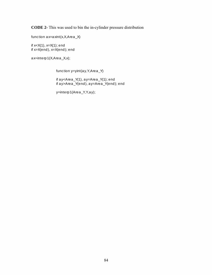
CODE 2- This was used to bin the in-cylinder pressure distribution function ax=axint(x,X,Area_X) if x<X(1), x=X(1); end if x>X(end), x=X(end); end ax=interp1(X,Area_X,x); function y=yint(ay,Y,Area_Y) if ay<Area_Y(1), ay=Area_Y(1); end if ay>Area_Y(end), ay=Area_Y(end); end y=interp1(Area_Y,Y,ay);

84

CODE 3- This code used in summing the area underneath the binned pressure distribution and creating accumulative sum. clear; % Loading data to matlab via excel columns [data,txt]=xlsread('Pressure Bins.xls','Pressure Bins'); x=data(:,1); % x axis of the X distribution y=data(:,1); % x axis of the Y distribution area_x=data(:,12); % y axis of the X distribution area_y=data(:,17); % y axis of the Y distribution figure(1) plot(x,area_x); figure(2) plot(y, area_y); figure(3) plot(x,yint(axint(x,x,area_x),y,area_y)); y_val=yint(axint(x,x,area_x),y,area_y); array=[x;(yint(axint(x,x,area_x),y,area_y))]; fido = fopen('cores.txt','a'); fprintf(fido,'%g %g \n',array); fprintf(fido,'\n'); fclose(fido);

85

CODE 4- This code was used to generate B-spline coefficients for the normalized accumulative summation graphs. lear all, clc, close all; dbstop error % Read in the data data1 = xlsread('Pressure Bins.xls','lifedata'); data = data1(:,15); x = [1:length(data)]'; % Cubic Bspline order = 4; % Generate knots of Bspline knots = linspace(1,length(data),2); knotsaug = augknt(knots, order); % Generate Bspline form sp = spap2(knotsaug,order,x,data); % sp = spap2(3,order,x,data); % Calculate the errors b/w the true data and the appoximated data errors = data-fnval(sp,x); % plot the true data and the appoximated data bspline=fnval(sp,x); fnplt(sp,'*'); figure(1) hold on, plot(x,data,'ro'),hold off; figure(2) plot(errors); % bspline([1 2 3 4 5]) % splinetool(x,data) % fnbrk(sp)

86

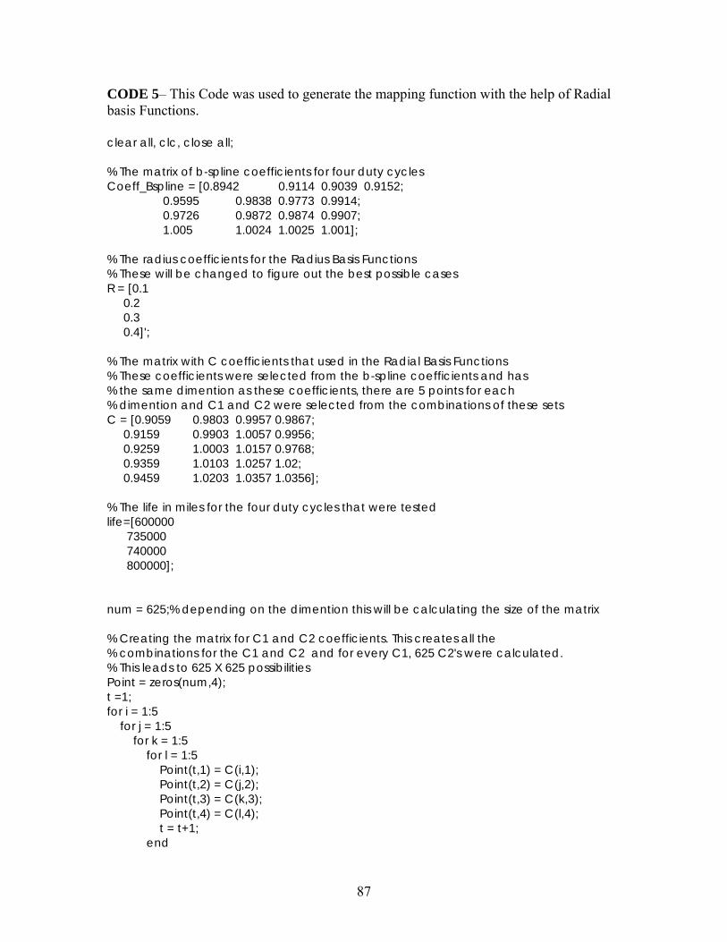
CODE 5– This Code was used to generate the mapping function with the help of Radial basis Functions. clear all, clc, close all; % The matrix of b-spline coefficients for four duty cycles Coeff_Bspline = [0.8942 0.9114 0.9039 0.9152; 0.9595 0.9838 0.9773 0.9914; 0.9726 0.9872 0.9874 0.9907; 1.005 1.0024 1.0025 1.001]; % The radius coefficients for the Radius Basis Functions % These will be changed to figure out the best possible cases R = [0.1 0.2 0.3 0.4]'; % The matrix with C coefficients that used in the Radial Basis Functions % These coefficients were selected from the b-spline coefficients and has % the same dimention as these coefficients, there are 5 points for each % dimention and C1 and C2 were selected from the combinations of these sets C = [0.9059 0.9803 0.9957 0.9867; 0.9159 0.9903 1.0057 0.9956; 0.9259 1.0003 1.0157 0.9768; 0.9359 1.0103 1.0257 1.02; 0.9459 1.0203 1.0357 1.0356]; % The life in miles for the four duty cycles that were tested life=[600000 735000 740000 800000]; num = 625;% depending on the dimention this will be calculating the size of the matrix % Creating the matrix for C1 and C2 coefficients. This creates all the % combinations for the C1 and C2 and for every C1, 625 C2's were calculated. % This leads to 625 X 625 possibilities Point = zeros(num,4); t =1; for i = 1:5 for j = 1:5 for k = 1:5 for l = 1:5 Point(t,1) = C(i,1); Point(t,2) = C(j,2); Point(t,3) = C(k,3); Point(t,4) = C(l,4); t = t+1; end

87

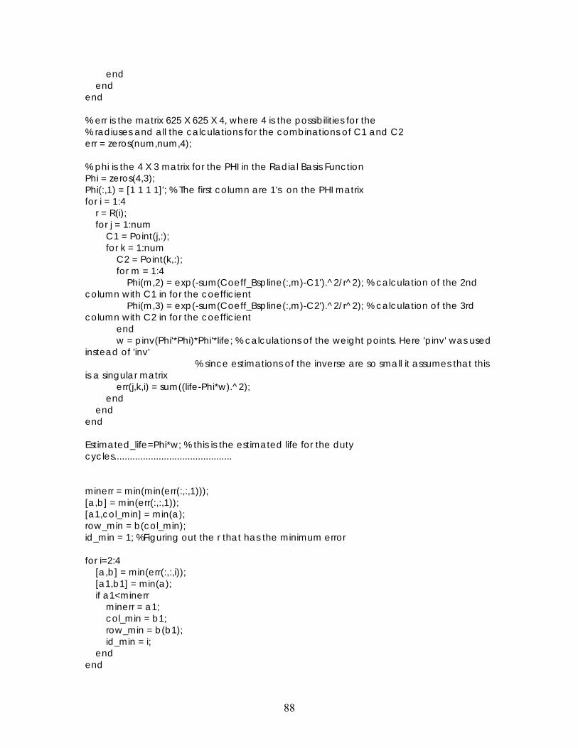
end end end % err is the matrix 625 X 625 X 4, where 4 is the possibilities for the % radiuses and all the calculations for the combinations of C1 and C2 err = zeros(num,num,4); % phi is the 4 X 3 matrix for the PHI in the Radial Basis Function Phi = zeros(4,3); Phi(:,1) = [1 1 1 1]'; % The first column are 1's on the PHI matrix for i = 1:4 r = R(i); for j = 1:num C1 = Point(j,:); for k = 1:num C2 = Point(k,:); for m = 1:4 Phi(m,2) = exp(-sum(Coeff_Bspline(:,m)-C1').^2/r^2); % calculation of the 2nd column with C1 in for the coefficient Phi(m,3) = exp(-sum(Coeff_Bspline(:,m)-C2').^2/r^2); % calculation of the 3rd column with C2 in for the coefficient end w = pinv(Phi'*Phi)*Phi'*life; % calculations of the weight points. Here 'pinv' was used instead of 'inv' % since estimations of the inverse are so small it assumes that this is a singular matrix err(j,k,i) = sum((life-Phi*w).^2); end end end Estimated_life=Phi*w; % this is the estimated life for the duty cycles............................................. minerr = min(min(err(:,:,1))); [a,b] = min(err(:,:,1)); [a1,col_min] = min(a); row_min = b(col_min); id_min = 1; %Figuring out the r that has the minimum error for i=2:4 [a,b] = min(err(:,:,i)); [a1,b1] = min(a); if a1<minerr minerr = a1; col_min = b1; row_min = b(b1); id_min = i; end end

88

C1_min = Point(row_min,:); C2_min = Point(col_min,:); r_min=id_min; save results

89

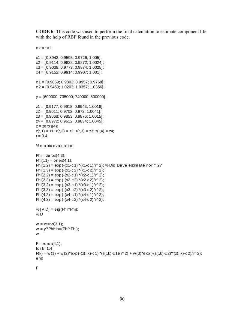
CODE 6- This code was used to perform the final calculation to estimate component life with the help of RBF found in the previous code. clear all x1 = [0.8942; 0.9595; 0.9726; 1.005]; x2 = [0.9114; 0.9838; 0.9872; 1.0024]; x3 = [0.9039; 0.9773; 0.9874; 1.0025]; x4 = [0.9152; 0.9914; 0.9907; 1.001]; c1 = [0.9059; 0.9803; 0.9957; 0.9768]; c2 = [0.9459; 1.0203; 1.0357; 1.0356]; y = [600000; 735000; 740000; 800000]; z1 = [0.9177; 0.9918; 0.9943; 1.0018]; z2 = [0.9011; 0.9702; 0.972; 1.0041]; z3 = [0.9068; 0.9853; 0.9876; 1.0015]; z4 = [0.8972; 0.9612; 0.9834; 1.0045]; z = zeros(4); z(:,1) = z1; z(:,2) = z2; z(:,3) = z3; z(:,4) = z4; r = 0.4; % matrix evaluation Phi = zeros(4,3); Phi(:,1) = ones(4,1); Phi(1,2) = exp(-(x1-c1)'*(x1-c1)/r^2); % Did Dave estimate r or r^2? Phi(1,3) = exp(-(x1-c2)'*(x1-c2)/r^2); Phi(2,2) = exp(-(x2-c1)'*(x2-c1)/r^2); Phi(2,3) = exp(-(x2-c2)'*(x2-c2)/r^2); Phi(3,2) = exp(-(x3-c1)'*(x3-c1)/r^2); Phi(3,3) = exp(-(x3-c2)'*(x3-c2)/r^2); Phi(4,2) = exp(-(x4-c1)'*(x4-c1)/r^2); Phi(4,3) = exp(-(x4-c2)'*(x4-c2)/r^2); % [V,D] = eig(Phi'*Phi); % D w = zeros(3,1); w = y'*Phi*inv(Phi'*Phi); w F = zeros(4,1); for k=1:4 F(k) = w(1) + w(2)*exp(-(z(:,k)-c1)'*(z(:,k)-c1)/r^2) + w(3)*exp(-(z(:,k)-c2)'*(z(:,k)-c2)/r^2); end F

90

CODE 7- A variation of Code 6, used to calculate the final life estimation. %These are the coefficients for the second set of duty cycles that were constructed. load results Coeff_Bspline2 = [0.9177; 0.9918; 0.9943; 1.0018]; Phi = zeros(4,3); Phi(:,1) = [1 1 1 1]'; % The first column are 1's on the PHI matrix Fr = 0.4; FC1 = C1_min; FC2 = C2_min; Phi1 = exp(-sum(Coeff_Bspline2-FC1').^2/(Fr^2)); % calculation of the 2nd column with C1 in for the coefficient Phi2 = exp(-sum(Coeff_Bspline2-FC2').^2/(Fr^2)); % calculation of the 3rd column with C2 in for the coefficient f = w(1)+w(2)*Phi1+w(3)*Phi2;

91