1Scientific RepoRts | 7:42872 | DOI: 10.1038/srep42872

www.nature.com/scientificreports

Effects of abiotic factors on ecosystem health of Taihu Lake, China based on eco-exergy theoryCe Wang1, Jun Bi1 & Brian D. Fath2,3

A lake ecosystem is continuously exposed to environmental stressors with non-linear interrelationships between abiotic factors and aquatic organisms. Ecosystem health depicts the capacity of system to respond to external perturbations and still maintain structure and function. In this study, we explored the effects of abiotic factors on ecosystem health of Taihu Lake in 2013, China from a system-level perspective. Spatiotemporal heterogeneities of eco-exergy and specific eco-exergy served as thermodynamic indicators to represent ecosystem health in the lake. The results showed the plankton community appeared more energetic in May, and relatively healthy in Gonghu Bay with both higher eco-exergy and specific eco-exergy; a eutrophic state was likely discovered in Zhushan Bay with higher eco-exergy but lower specific eco-exergy. Gradient Boosting Machine (GBM) approach was used to explain the non-linear relationships between two indicators and abiotic factors. This analysis revealed water temperature, inorganic nutrients, and total suspended solids greatly contributed to the two indicators that increased. However, pH rise driven by inorganic carbon played an important role in undermining ecosystem health, particularly when pH was higher than 8.2. This implies that climate change with rising CO2 concentrations has the potential to aggravate eutrophication in Taihu Lake where high nutrient loads are maintained.

Water quality management can best be upgraded to aquatic ecosystem health assessment by evaluating multiple environmental stressors that can potentially impair ecosystem structure and function and further undermine ecosystem goods and services. Plankton communities play a significant role in establishing aquatic ecosystems, of which the primary producer, phytoplankton, initiates energy flow and chemical cycling driven by solar radiation, and the primary consumer, zooplankton, largely feeds on phytoplankton, in general, with an inverse relation-ship between their densities because of predator-prey interaction1,2. Together, they constitute the food source for many aquatic organisms in higher trophic levels, e.g., fish species. Particularly, for eutrophication management in shallow lakes under external stress, a hysteresis phenomenon is observed in the plankton community such that the system remains on the same state until a catastrophic bifurcation is reached at which it shifts to the alterna-tive state3,4. Catastrophic regime shift has drawn more attention since it can result in loss of species, functions, ecosystem services, ecological, and economic resources and might fundamentally degrade aquatic ecosystem health5. Therefore, it is important to apply an integrated system-level indicator to assess the variation trend of lake ecosystem health imposed by external forcing functions6–9.

Exergy, a thermodynamic concept, represents the potential for a given amount of energy to perform work to bring the system to thermodynamic equilibrium10,11. Studies of ecological systems also include an exergy weight-ing factor, β , to account for the information embedded in the species genetic complexity12. The species-specific β -value is the work energy of an organism including the information relative to the work energy (exergy) with only the biomass chemical exergy. Hence, an organism without information is considered as a fuel which can-not display direct life processes13. An ecosystem can utilize input of eco-exergy to increase biomass and further move away from thermodynamic equilibrium by ecological network development and information increase14. Eco-exergy could be considered as a holistic ecological indicator of ecosystem development, health and also eco-system services15,16, e.g., tropical rainforest (3200 kEURO/ha per year) presented more valuable than desert (20.7 kEURO/ha per year) based on eco-exergy calculation. Specific eco-exergy (also called structural eco-exergy)

1State Key Laboratory of Pollution Control and Resource Reuse, School of the Environment, Nanjing University, Nanjing, 210023, P.R. China. 2Biology Department, Towson University, Towson, MD 21252, USA. 3Advanced Systems Analysis Program, International Institute for Applied Systems Analysis (IIASA), Laxenburg, Austria. Correspondence and requests for materials should be addressed to J.B. (email: jbi@nju.edu.cn) or B.D.F. (email: bfath@towson.edu)

Received: 18 August 2016

Accepted: 17 January 2017

Published: 21 February 2017

OPEN

www.nature.com/scientificreports/

2Scientific RepoRts | 7:42872 | DOI: 10.1038/srep42872

reflecting the ability of an ecosystem to utilize available resources is defined as the ratio of eco-exergy to total bio-mass. It gives us the composition of the ecosystem (the more developed organisms the higher specific eco-exergy) and therefore it is a good indicator for ecosystem health assessment, particularly when we focus on lake eutroph-ication17. Therefore, we supplement the use of eco-exergy with specific eco-exergy indictors to assess lake ecosys-tem health under external stress.

It is very difficult to elucidate the detailed mechanisms on how a lake ecosystem responds to changing envi-ronmental and anthropogenic pressures because of the ecosystem complexity that includes nonlinear interactions and heterogeneity among components18–20. Therefore, we need a simple and effective mathematical approach to determine ecosystem health changes resulting from external perturbations. Gradient Boosting Machine (GBM) is a decision-tree based approach coupling with a gradient boost algorithm to make accurate estimations of the response variable among highly non-linear relationships in the system of interest, and the principal of the algorithm is to establish new base-learners to be maximally correlated with the negative gradient of the loss function21,22. Meanwhile, the method can also illustrate the marginal effect of the selected independent variable on the response variable while all other covariates were kept constant at their observations using a partial dependence plot23. This kind of modeling has been successfully applied into ecology and biology for simulating non-linear interactions between response and predictor variables24–27. E.g., Randall and Van Woesik 28 investigated the effect of eight sea surface temperature metrics on white-band disease of reef-building corals in the Caribbean, indicating that the dis-ease was associated with climate change, which resulted in the regional population decline. Based on the complexity among components in a lake, GBM can improve the prediction of ecosystem health by combining information from many abiotic factors that individually may not be significant but together are very influential. Using GBM analysis we aim to examine the influence of abiotic factors, e.g., nutrients, temperature, and solar radiation, on the eco-exergy densities of the plankton community to obtain insights into how the ecosystem health of a shallow lake varies.

In this study, we aim to calculate eco-exergy and specific eco-exergy indicators of plankton community at 33 sampling sites in Taihu Lake using monthly-measured phytoplankton and zooplankton biomass during 2013 to illustrate spatiotemporal variation of health level and plankton community dynamics, then apply GBM to determine the effects of abiotic factors on lake ecosystem health. The quantitative relationship between ecological indicators and environmental parameters will help us to predict ecosystem health changes in a shallow lake.

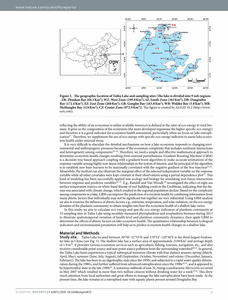
Material and MethodsStudy site. Taihu Lake located between 30°56′ -31°33′ N and 119°53′ -120°36′ E is the third largest freshwa-ter lake in China (see Fig. 1). The shallow lake has a surface area of approximately 2338 Km2 and average depth of 1.9 m29. It provides various ecosystem services such as agriculture, fishing, tourism, navigation, etc., and also receives considerable point-source and non-point source pollution from the surrounding watershed30,31. In general, the Taihu Lake basin experiences a typical subtropical monsoon climate with four distinct seasons: spring (March, April, May), summer (June, July, August), fall (September, October, November) and winter (December, January, February). The lake has been in an oligotrophic state since the 1950 s and subjected to a rapid water quality deterio-ration during the 1980 s, and further suffered from advanced eutrophication since the 1990s32,33, and it appeared to be hypertrophic state in the late 1990s34. A notorious outbreak of non-N2-fixing cyanobacteria Microcystis occurred in May 2007 which resulted in more than two million citizens without drinking water for a week35,36. This drew much attention from local authorities and great efforts to manage the lake eutrophication have been made. At the present time, the lake remains in a eutrophied state with aquatic plants present around Dongtaihu Bay.

Figure 1. The geographic location of Taihu Lake and sampling sites (The lake is divided into 9 sub-regions - ZB: Zhushan Bay (68.3 Km2); WZ: West Zone (199.8 Km2); SZ: South Zone (363 Km2); DB: Dongtaihu Bay (172.4 Km2); EZ: East Zone (268 Km2); GB: Gonghu Bay (163.8 Km2); WB: Wulihu Bay (5.8 Km2); MB: Meilianghu Bay (124 Km2); CZ: Center Zone (972.9 Km2)). The figure is created by ArcGIS 10.2 (http://www.esri.com).

www.nature.com/scientificreports/

3Scientific RepoRts | 7:42872 | DOI: 10.1038/srep42872

Sample collection. Field measurements of the lake ecosystem were regularly carried out at monthly inter-vals in 2013 at 33 sampling locations in Taihu Lake, as shown in Fig. 1. The 33 sampling locations belong to nine sub-regions, namely Zhushan Bay (ZB, two stations), West Zone (WZ, two stations), South Zone (SZ, five stations), Dongtaihu Bay (DB, three stations), East Zone (EZ, four stations), Gonghu Bay (GB, four stations), Wulihu Bay (WB, three stations), Meilianghu Bay (MB, four stations) and Center Zone (CZ, six stations). On the first ten-day period of each month, we collected water samples at a depth of 0.5 m at each site by driving a vessel with the help of an instrument of navigation-GPS. For each field investigation, approximately 10–12 sampling locations could be visited.

Ammonia nitrogen (NH4-N), nitrite nitrogen (NO2-N), nitrate nitrogen (NO3-N), total nitrogen (TN), orthophosphate (PO4-P), dissolved total phosphorous (DTP), total phosphorous (TP), Chlorophyll-a (Chla) and total suspend solids (TSS) concentrations were determined by laboratory analysis within 24 h after sampling. Dissolved oxygen (DO), water temperature (WTEMP), pH, secchi disc depth (SDD) and wind speed (WIND) were directly measured on the spot using a portable monitoring device. Water depth (WD) at each site was cal-culated by subtracting lake bed elevation from the lake water level. During 2013, in the whole lake, we identified a total of 139 species of phytoplankton (Phyt), of which the dominant species were Chlorophyta, Bacillariophyta and Cyanophyta; meanwhile, 102 species of zooplankton (Zoop) were observed, of which the protozoa were the most abundant in number count while cladocera and copepoda had the largest biomass. All of phytoplankton and zooplankton biomass were measured in wet weight. Meteorological data of precipitation (PREC) in Wuxi city and solar radiation (SOLR) in Nanjing city stations were obtained from the China Meteorological Data Sharing Service System of the National Meteorological Information Center. Due to constrained resources, PREC and SOLR observations in time series from respective meteorological station were assumed to be representa-tive of the whole lake, while all other water quality, ecological and meteorological data were determined syn-chronously for each sampling time and site. The detailed information on water sampling, sample pretreatment and laboratory analysis with defined methods for environmental protection standards of China were listed in Supplement Material, Section 1 and Section 2.

Eco-exergy and specific eco-exergy estimates of plankton community. To calculate eco-exergy, we multiplied the biomass concentration of an organism in the plankton community by the corresponding β -value37,38. Empirical conversion factors were used to convert wet weight to dry weight biomass in carbon unit (also see Supplementary Material). Using the C-biomass concentrations, we calculated the eco-exergy density measuring per volume eco-exergy. At each sampling date and site, we summed all eco-exergy densities of phy-toplankton and zooplankton species to obtain an overall index for the plankton community (see Equation (1)). Then, specific eco-exergy was expressed by eco-exergy per unit of total C-biomass of plankton community (see Equation (2)).

∑ ∑ ∑ ∑

∑

β β β β

β

= . ×

+ + +

+

_= = = =

=

E f C f C f C f C

f C

18 7

(1)

X ECO algi

N

phy phy i proj

M

zoo pro j rotj

L

zoo rot j claj

K

zoo cla j

copj

H

zoo cop j

1,

1,

1,

1,

1,

=__E

EBiomass (2)X SP

X ECO

total

where _EX ECO [J/L] is eco-exergy density expressed in detritus equivalent; βalg, βpro, βrot, βcla and βcop [dimension-less] are 20, 39, 163, 232 and 232 for planktonic algae, zooplankton - protozoa, rotifers, cladocera and copepoda, respectively12. Cphy, i, Cpro, j, Crot, j, Ccla, j and Ccop, j [mg/L] represent the wet weight biomass of the ith phytoplankton species and the jth zooplankton species, respectively. fphy and fzoo are 0.16 and 0.06 served as the conversion factors of wet weight to C-biomass for phytoplankton and zooplankton species, respectively39–42; The multiplier factor of 18.7 kJ/g changes _EX ECO into the energy expressed as organic matter equivalent energy, because the average eco-exergy of detritus is 18.7 kJ/g. N, M, L, K and H are equal to the number of phytoplankton and zooplankton species, respectively. _EX SP [kJ/g] is specific eco-exergy and Biomasstotal [mg/L] is the sum of phytoplankton and zooplankton C-biomass in dry weight. Statistical results for _EX ECO and _EX SP calculations cannot be affected, although systematic errors are yield as function of empirical values of dry weight.

Gradient Boosting Machine and model evaluation. GBM analysis was performed on the key ecologi-cal indictors, namely EX_ECO and EX_SP, using the variables filtered by Pearson correlation coefficients to avoid correlation levels higher than 0.724. In our model we specified a Gaussian loss function with a 5-fold cross valida-tion and the number of iterations set to 1500, an interaction depth of 5, and a learning rate of 0.005. A compre-hensive introduction to this technique with parameterization is available43,44. The model was fitted using the R statistical package45. The Chla parameter was not shown in the list of independent covariates since the concentra-tions belonging to phytoplankton biomass were used to calculate EX_ECO and EX_SP indicators. The model perfor-mance was evaluated using four quantitative statistical methods: coefficient of determination (R2), Nash-Sutcliffe efficiency (NSE), ratio of the root-mean-square to the standard deviation of measured data (RSR), and percent bias (PBIAS), and the model prediction was judged as agreeable if NSE > 0.5, RSR ≤ 0.7 and PBIAS∈[− 25%, 25%]46,47. The whole process of modeling was illustrated in Supplementary Material, Section 3.

www.nature.com/scientificreports/

4Scientific RepoRts | 7:42872 | DOI: 10.1038/srep42872

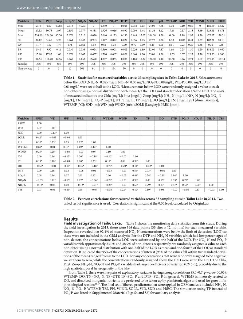
ResultsField investigation of Taihu Lake. Table 1 shows the monitoring data statistics from this study. During the field investigation in 2013, there were 396 data points (33 sites × 12 months) for each measured variable. Inspection revealed that 92.4% of measured NO2-N concentrations were below the limit of detection (LOD) so these were not included in the GBM analysis. For the DTP and NH4-N variables which had low percentages of non-detects, the concentrations below LOD were substituted by one-half of the LOD. For NO3-N and PO4-P variables with approximately 23.0% and 38.9% of non-detects respectively, we randomly assigned a value to each non-detect using a normal distribution with one-half of the LOD as mean and one-fourth of the LOD as standard deviation. It indicated that 95% of the concentrations of interest (95% of the values fell within two standard devia-tions of the mean) ranged from 0 to the LOD. For any concentrations that were randomly assigned to be negative, we set them to zero, while the concentrations randomly assigned above the LOD were set to the LOD. The Chla, Phyt, Zoop, NH4-N, NO3-N and PO4-P variables had larger coefficients of variation (CV > 1), probably due to the high spatiotemporal heterogeneity in the lake.

From Table 2, there were five pairs of explanatory variables having strong correlations (R > 0.7, p-value < 0.05): WTEMP~DO, TN~NO3-N, TP~DTP, TP~PO4-P and DTP~PO4-P. In general, WTEMP is inversely related to DO, and dissolved inorganic nutrients are preferred to be taken up by planktonic algae and used for growth for physiological reasons48,49. The final set of filtered predicators that were applied in GBM analysis included NH4-N, NO3-N, PO4-P, WTEMP, TSS, PH, WIND, SOLR, WD, SDD and PREC. The simulation using TP instead of PO4-P was listed in Supplemental Material (Figs S4 and S5) for auxiliary analysis.

Variables Chla Phyt Zoop NH4-Na NO2-N NO3-Nb TN PO4-Pb DTPa TP DO TSS pH WTEMP SDD WD WIND SOLR PREC

Min 2.10 0.67 0.058 0.013 < 0.03 0 0.340 0 0.005 0.018 3.03 24.00 7.56 1.30 0.10 0.89 0 186.69 13.22

Mean 27.52 30.78 2.97 0.150 0.077 0.881 1.926 0.016 0.030 0.080 9.44 61.36 8.42 17.68 0.37 2.18 3.69 323.15 88.71

Max 238.00 224.00 45.30 2.070 0.210 4.070 7.060 0.173 0.190 0.448 13.07 164.00 9.58 34.60 1.18 2.97 9.20 472.67 178.51

SD 32.12 34.60 5.26 0.264 0.043 0.903 1.177 0.022 0.027 0.056 1.75 27.77 0.38 8.93 0.086 0.44 1.39 102.31 60.18

CV 1.17 1.12 1.77 1.76 0.562 1.03 0.61 1.38 0.90 0.70 0.19 0.45 0.05 0.51 0.23 0.20 0.38 0.32 0.68

P5 5.40 3.92 0.14 0.030 0.033 0.024 0.560 0.001 0.005 0.026 6.89 32.00 7.87 1.60 0.28 1.30 1.20 188.03 13.60

P50 15.80 17.95 1.00 0.070 0.067 0.637 1.700 0.007 0.021 0.066 9.20 53.00 8.38 18.35 0.37 2.27 3.70 323.33 92.06

P95 94.64 111.70 12.56 0.460 0.152 2.620 4.297 0.065 0.088 0.184 12.22 124.00 9.10 30.60 0.46 2.74 5.87 471.15 177.14

Samples 396 396 396 396 396 396 396 396 396 396 396 396 396 396 396 396 396 396 396

Non-detects 0 0 0 10 366 91 0 154 30 0 0 0 0 0 0 0 0 0 0

Table 1. Statistics for measured variables across 33 sampling sites in Taihu Lake in 2013. aMeasurements below the LOD (NH4-N: 0.025 mg/L; NO2-N: 0.03 mg/L; NO3-N: 0.08 mg/L; PO4-P: 0.005 mg/L; DTP: 0.01 mg/L) were set to half to the LOD. bMeasurements below LOD were randomly assigned a value to each non-detect using a normal distribution with mean 1/2 the LOD and standard deviation 1/4 the LOD. The units of measured indicators are: Chla [mg/L]; Phyt [mg/L]; Zoop [mg/L]; NH4-N [mg/L]; NO2-N [mg/L]; NO3-N [mg/L]; TN [mg/L]; PO4-P [mg/L]; DTP [mg/L]; TP [mg/L]; DO [mg/L]; TSS [mg/L]; pH [dimensionless], WTEMP [°C]; SDD [m]; WD [m]; WIND [m/s]; SOLR [Langley]; PREC [mm].

Variables PREC WD SDD SOLR PH WTEMP WIND TN TP DO DTP PO4-P NO3-N NH4-N TSS

PREC 1.00

WD 0.07 1.00

SDD 0.00 − 0.13* 1.00

SOLR 0.41* − 0.01 − 0.08 1.00

PH 0.10* 0.25* 0.05 0.12* 1.00

WTEMP 0.60* 0.01 0.10* 0.69* 0.44* 1.00

WIND 0.25* 0.20* − 0.03 − 0.07 0.07 0.10 1.00

TN 0.00 0.16* − 0.15* 0.20* − 0.18* − 0.20* − 0.02 1.00

TP 0.19* 0.18* − 0.09 0.10* 0.33* 0.17* 0.00 0.39* 1.00

DO − 0.57* − 0.01 − 0.19* − 0.45* − 0.18* − 0.78* − 0.20* 0.14* − 0.12* 1.00

DTP 0.09 0.16* 0.02 − 0.06 0.04 − 0.03 − 0.01 0.54* 0.73* − 0.01 1.00

PO4-P 0.08 0.16* 0.07 0.00 0.12* 0.06 − 0.05 0.48* 0.74* − 0.10* 0.94* 1.00

NO3-N − 0.09 0.12* − 0.15* 0.17* − 0.36* − 0.29* − 0.01 0.90* 0.08 0.15* 0.33* 0.27* 1.00

NH4-N − 0.12* 0.03 0.00 − 0.12* − 0.21* − 0.26* − 0.03 0.65* 0.29* 0.13* 0.57* 0.52* 0.50* 1.00

TSS 0.07 0.04 − 0.29* 0.09 − 0.07 − 0.08 0.22* 0.12* 0.19* 0.00 − 0.07 − 0.06 0.13* − 0.03 1.00

Table 2. Pearson correlations for measured variables across 33 sampling sites in Taihu Lake in 2013. Two-tailed test of significance is used. *Correlation is significant at the 0.05 level, calculated by OriginLab.

www.nature.com/scientificreports/

5Scientific RepoRts | 7:42872 | DOI: 10.1038/srep42872

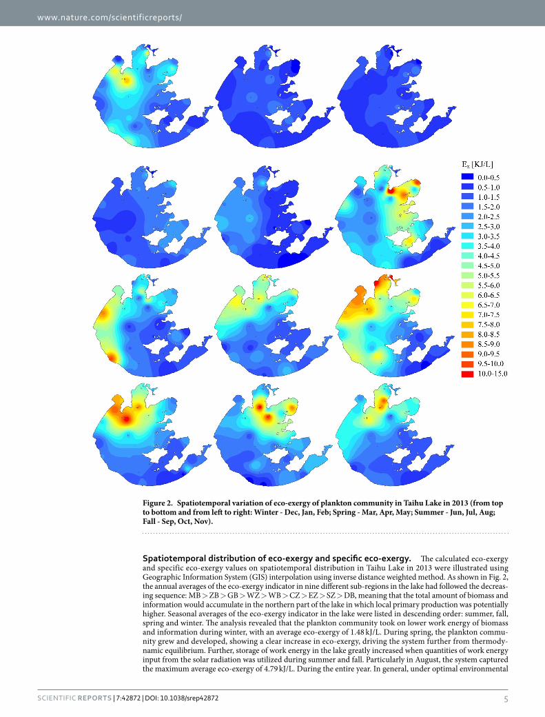
Spatiotemporal distribution of eco-exergy and specific eco-exergy. The calculated eco-exergy and specific eco-exergy values on spatiotemporal distribution in Taihu Lake in 2013 were illustrated using Geographic Information System (GIS) interpolation using inverse distance weighted method. As shown in Fig. 2, the annual averages of the eco-exergy indicator in nine different sub-regions in the lake had followed the decreas-ing sequence: MB > ZB > GB > WZ > WB > CZ > EZ > SZ > DB, meaning that the total amount of biomass and information would accumulate in the northern part of the lake in which local primary production was potentially higher. Seasonal averages of the eco-exergy indicator in the lake were listed in descending order: summer, fall, spring and winter. The analysis revealed that the plankton community took on lower work energy of biomass and information during winter, with an average eco-exergy of 1.48 kJ/L. During spring, the plankton commu-nity grew and developed, showing a clear increase in eco-exergy, driving the system further from thermody-namic equilibrium. Further, storage of work energy in the lake greatly increased when quantities of work energy input from the solar radiation was utilized during summer and fall. Particularly in August, the system captured the maximum average eco-exergy of 4.79 kJ/L. During the entire year. In general, under optimal environmental

Figure 2. Spatiotemporal variation of eco-exergy of plankton community in Taihu Lake in 2013 (from top to bottom and from left to right: Winter - Dec, Jan, Feb; Spring - Mar, Apr, May; Summer - Jun, Jul, Aug; Fall - Sep, Oct, Nov).

www.nature.com/scientificreports/

6Scientific RepoRts | 7:42872 | DOI: 10.1038/srep42872

conditions eco-exergy increases due to zooplankton growth from abundance of phytoplankton. However, the lake suffered from eutrophication due to the massive propagation of planktonic algae during the second half of 2013 (see Fig. 3). When the lake eutrophication emerged, we do have more biomass of phytoplankton for a time and the eco-exergy to measure biomass and information increased as well. Therefore, we cannot judge whether the aquatic ecosystem’s health is only based on the eco-exergy indicator.

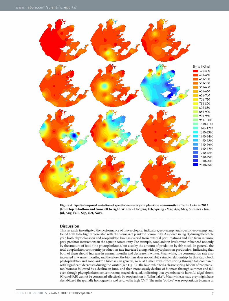
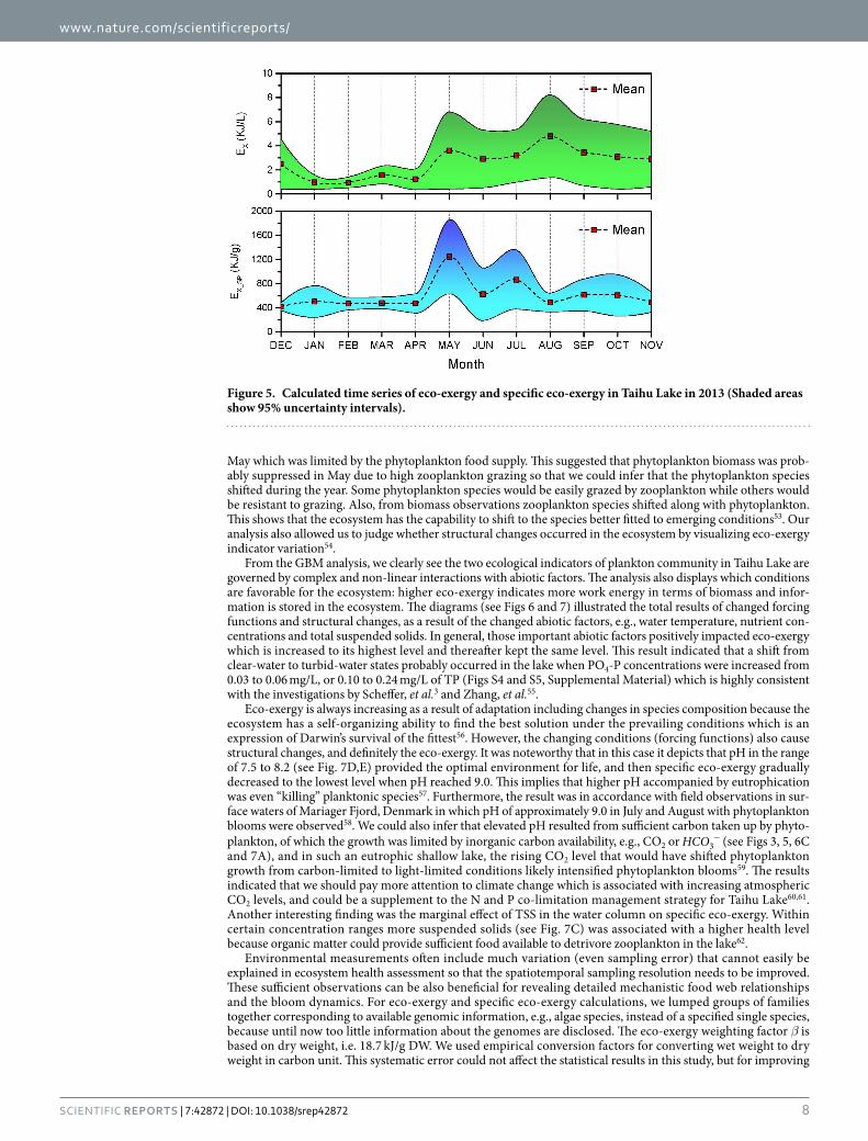
The specific eco-exergy indictor which expressed the dominance of the higher organisms carrying more infor-mation per unit of biomass was applied to assess lake ecosystem health50. The annual averages of the specific eco-exergy indicator in nine different sub-regions in the lake had followed the increasing sequence: ZB < WB < WZ < SZ < MB < CZ < DB < GB < EZ (see Fig. 4). Compared with eco-exergy values, Zhushan Bay had a great potential for eutrophication in that it exhibited a very high exergy but low specific eco-exergy, indicating that the biomass would be dominated by planktonic algae with low β-values. In general, Gonghu Bay presented a more healthy status as both eco-exergy (3.46 kJ/L) and specific eco-exergy (676.0 kJ/g) were relatively high in compar-ison with the other counterparts. As evidenced by both ecological indicators reaching the high level, as shown in Fig. 5, the lake remained healthy in May. From the time-varying trends, in August the plankton community with increasing eco-exergy but decreasing specific eco-exergy implied that the lake was prone to be eutrophic. It could also be demonstrated in Fig. 3 that phytoplankton biomass was in the highest level in August in 2013.

Effects of abiotic factors on eco-exergy and specific eco-exergy. Both eco-exergy and specific eco-exergy were satisfactorily predicted by non-linear relationships with multiple abiotic factors. The statistical analysis resulted in values of 0.784 and 0.710 of R2, 0.77 and 0.69 of NES, 0.49 and 0.55 of RSR, and − 8.7% and − 4.6% of PBIAS for eco-exergy and specific eco-exergy, respectively (see Figs S2 and S3, Supplemental Material). For each ecological indicator, the top three variables having the highest relative influence together explained over 50% of the model variability. As shown in Fig. 6A–C, eco-exergy experienced a notable increase at water temper-ature higher than 16 °C, and a gradual increase over 20 °C. For dissolved inorganic nutrients, above the threshold of 1.75 μ g/L of PO4-P, small increases in nutrient concentrations resulted in a dramatic increases in eco-exergy, followed by a plateau at higher concentrations. Increasing PH, in general, resulted in the elevated eco-exergy. Obviously, interaction analysis illustrated the interactive effect of any two-variable pair of WTEMP, PO4-P and PH on eco-exergy. Particularly, eco-exergy reached the highest level at moderate PH and PO4-P concentrations (see Fig. 6D–F).

Specific eco-exergy was largely explained by PH (15.5%), WTEMP (18.7%) and TSS (19.2%) (see Fig. 7A–C). Slight increases in pH up to 8.2 predicted an almost linear decline in the specific eco-exergy. Again, specific eco-exergy increased gradually at low WTEMP, tipping at 17 °C and then started escalating, and finally kept steady above 20 °C. Specific eco-exergy was approximately directly proportional to TSS, however there was a flat relationship after TSS concentration reached 115 mg/L. The relationship between WTEMP and specific eco-exergy was weak at higher PH whereas decreased PH resulted in elevated specific eco-exergy at high WTEMP (Fig. 7D–F). At lower TSS and WTEMP (rising PH), the relationship between specific eco-exergy and the two variables were relatively inactive, however, elevated TSS and WTEMP (falling PH) was associated with increasing specific eco-exergy with two sharp thresholds. From Figs 6C and 7A, it was clearly shown that higher pH probably triggered propagation of planktonic algae.

Figure 3. Time series of monthly observed phytoplankton and zooplankton biomass across 33 sampling sites in Taihu Lake in 2013 (Box and whisker represent 25th–75th and 5th–95th respectively; line within box represents median; quadrate within box represents mean; triangle and reverse triangle represent 1th and 99th respectively; upper and lower short strings represent maximum and minimum respectively).

www.nature.com/scientificreports/

7Scientific RepoRts | 7:42872 | DOI: 10.1038/srep42872

DiscussionThis research investigated the performance of two ecological indicators, eco-exergy and specific eco-exergy and found both to be highly correlated with the biomass of plankton community. As shown in Fig. 3, during the whole year, both phytoplankton and zooplankton biomass varied from external perturbations and also from intrinsic prey-predator interactions in the aquatic community. For example, zooplankton levels were influenced not only by the amount of food (the phytoplankton), but also by the amount of predation by fish stock. In general, the total zooplankton community production rate increased along with phytoplankton production, indicating that both of them should increase in warmer months and decrease in winter. Meanwhile, the consumption rate also increased in warmer months, and therefore, the biomass does not exhibit a simple relationship. In this study, both phytoplankton and zooplankton biomass, in general, were at higher levels from spring through fall compared with significant decreases during the winter (see Fig. 3). The lake exhibited a classic spring bloom of zooplank-ton biomass followed by a decline in June, and then more steady decline of biomass through summer and fall even though phytoplankton concentrations stayed elevated, indicating that cyanobacteria harmful algal bloom (CyanoHAB) cannot be consumed effectively by zooplankton in Taihu Lake51. Meanwhile, a toxic prey might have destabilized the spatially homogeneity and resulted in high CV52. The main “outlier” was zooplankton biomass in

Figure 4. Spatiotemporal variation of specific eco-exergy of plankton community in Taihu Lake in 2013 (from top to bottom and from left to right: Winter - Dec, Jan, Feb; Spring - Mar, Apr, May; Summer - Jun, Jul, Aug; Fall - Sep, Oct, Nov).

www.nature.com/scientificreports/

8Scientific RepoRts | 7:42872 | DOI: 10.1038/srep42872

May which was limited by the phytoplankton food supply. This suggested that phytoplankton biomass was prob-ably suppressed in May due to high zooplankton grazing so that we could infer that the phytoplankton species shifted during the year. Some phytoplankton species would be easily grazed by zooplankton while others would be resistant to grazing. Also, from biomass observations zooplankton species shifted along with phytoplankton. This shows that the ecosystem has the capability to shift to the species better fitted to emerging conditions53. Our analysis also allowed us to judge whether structural changes occurred in the ecosystem by visualizing eco-exergy indicator variation54.

From the GBM analysis, we clearly see the two ecological indicators of plankton community in Taihu Lake are governed by complex and non-linear interactions with abiotic factors. The analysis also displays which conditions are favorable for the ecosystem: higher eco-exergy indicates more work energy in terms of biomass and infor-mation is stored in the ecosystem. The diagrams (see Figs 6 and 7) illustrated the total results of changed forcing functions and structural changes, as a result of the changed abiotic factors, e.g., water temperature, nutrient con-centrations and total suspended solids. In general, those important abiotic factors positively impacted eco-exergy which is increased to its highest level and thereafter kept the same level. This result indicated that a shift from clear-water to turbid-water states probably occurred in the lake when PO4-P concentrations were increased from 0.03 to 0.06 mg/L, or 0.10 to 0.24 mg/L of TP (Figs S4 and S5, Supplemental Material) which is highly consistent with the investigations by Scheffer, et al.3 and Zhang, et al.55.

Eco-exergy is always increasing as a result of adaptation including changes in species composition because the ecosystem has a self-organizing ability to find the best solution under the prevailing conditions which is an expression of Darwin’s survival of the fittest56. However, the changing conditions (forcing functions) also cause structural changes, and definitely the eco-exergy. It was noteworthy that in this case it depicts that pH in the range of 7.5 to 8.2 (see Fig. 7D,E) provided the optimal environment for life, and then specific eco-exergy gradually decreased to the lowest level when pH reached 9.0. This implies that higher pH accompanied by eutrophication was even “killing” planktonic species57. Furthermore, the result was in accordance with field observations in sur-face waters of Mariager Fjord, Denmark in which pH of approximately 9.0 in July and August with phytoplankton blooms were observed58. We could also infer that elevated pH resulted from sufficient carbon taken up by phyto-plankton, of which the growth was limited by inorganic carbon availability, e.g., CO2 or −HCO3 (see Figs 3, 5, 6C and 7A), and in such an eutrophic shallow lake, the rising CO2 level that would have shifted phytoplankton growth from carbon-limited to light-limited conditions likely intensified phytoplankton blooms59. The results indicated that we should pay more attention to climate change which is associated with increasing atmospheric CO2 levels, and could be a supplement to the N and P co-limitation management strategy for Taihu Lake60,61. Another interesting finding was the marginal effect of TSS in the water column on specific eco-exergy. Within certain concentration ranges more suspended solids (see Fig. 7C) was associated with a higher health level because organic matter could provide sufficient food available to detrivore zooplankton in the lake62.

Environmental measurements often include much variation (even sampling error) that cannot easily be explained in ecosystem health assessment so that the spatiotemporal sampling resolution needs to be improved. These sufficient observations can be also beneficial for revealing detailed mechanistic food web relationships and the bloom dynamics. For eco-exergy and specific eco-exergy calculations, we lumped groups of families together corresponding to available genomic information, e.g., algae species, instead of a specified single species, because until now too little information about the genomes are disclosed. The eco-exergy weighting factor β is based on dry weight, i.e. 18.7 kJ/g DW. We used empirical conversion factors for converting wet weight to dry weight in carbon unit. This systematic error could not affect the statistical results in this study, but for improving

Figure 5. Calculated time series of eco-exergy and specific eco-exergy in Taihu Lake in 2013 (Shaded areas show 95% uncertainty intervals).

www.nature.com/scientificreports/

9Scientific RepoRts | 7:42872 | DOI: 10.1038/srep42872

accuracy it will be necessary to obtained site-specific plankton dry weight biomass based on laboratory analysis. Furthermore, to better assess ecosystem health, benthos, macrophytes (the abundance of macrophytes is decreas-ing) and fish species in the lake should also be included.

Figure 6. Single-variable and two-variable partial dependence plots for the three most influential predictor variables of eco-exergy in GBM model.

Figure 7. Single-variable and two-variable partial dependence plots for the three most influential predictor variables of specific eco-exergy in GBM model.

www.nature.com/scientificreports/

1 0Scientific RepoRts | 7:42872 | DOI: 10.1038/srep42872

Ecological systems may undergo catastrophic shifts, which abruptly shifts from one state to a contrasting one, across a tipping point as a result of changing external conditions, leading to substantial loss of ecosystem services63,64. Therefore, it is important to detect early-warning signals for critical transitions so that quick and effective management action can be implemented to prevent the “collapse”. On the one hand, based on eco-exergy theory and sufficient observations, we might judge the system behavior that might undergo development, suc-cession and modification when exposed to variation in environmental conditions65,66. On the other hand, we also recommend that eco-exergy and specific eco-exergy indicators be applied to calculate statistical early warning signals such as variance, return rate and skewness to predict regime shifts from oligotrophic to hypertrophic state in Taihu Lake during the past six decades, using either long-term temporal or high-resolution spatial mon-itoring data67,68. Unfortunately, relevant research on anticipating critical transitions using these two ecological indicators has been scarce, possibly due to limited data availability. However, connecting eco-exergy theory with catastrophic theory opens up obvious new perspectives in the field of aquatic ecology, including ecosystem health assessments of shallow lakes worldwide.

References1. Reece, J. et al. Campbell biology. (Pearson Higher Education AU, 2011).2. Medvinsky, A. B., Petrovskii, S. V., Tikhonova, I. A., Malchow, H. & Li, B.-L. Spatiotemporal complexity of plankton and fish

dynamics. Siam Review 44, 311–370 (2002).3. Scheffer, M., Carpenter, S., Foley, J. A., Folke, C. & Walker, B. Catastrophic shifts in ecosystems. Nature 413, 591–596 (2001).4. Scheffer, M. & Carpenter, S. R. Catastrophic regime shifts in ecosystems: linking theory to observation. Trends Ecol Evol 18, 648–656,

doi: 10.1016/j.tree.2003.09.002 (2003).5. Kéfi, S., Dakos, V., Scheffer, M., Van Nes, E. H. & Rietkerk, M. Early warning signals also precede non-catastrophic transitions. Oikos

122, 641–648 (2013).6. Scheffer, M. & Jeppesen, E. Regime shifts in shallow lakes. Ecosystems 10, 1–3 (2007).7. Ibelings, B. W. et al. Resilience of alternative stable states during the recovery of shallow lakes from eutrophication: Lake Veluwe as

a case study. Ecosystems 10, 4–16 (2007).8. Dai, L., Vorselen, D., Korolev, K. S. & Gore, J. Generic indicators for loss of resilience before a tipping point leading to population

collapse. Science 336, 1175–1177 (2012).9. Jørgensen, S. E., Xu, L. & Costanza, R. Handbook of ecological indicators for assessment of ecosystem health. (CRC press, 2010).

10. Ulanowicz, R. E., Jørgensen, S. E. & Fath, B. D. Exergy, information and aggradation: An ecosystems reconciliation. Ecol Model 198, 520–524, doi: 10.1016/j.ecolmodel.2006.06.004 (2006).

11. Ludovisi, A. & Jørgensen, S. E. Comparison of exergy found by a classical thermodynamic approach and by the use of the information stored in the genome. Ecol Model 220, 1897–1903, doi: 10.1016/j.ecolmodel.2009.04.019 (2009).

12. Jørgensen, S. E., Ladegaard, N., Debeljak, M. & Marques, J. C. Calculations of exergy for organisms. Ecol Model 185, 165–175, doi: 10.1016/j.ecolmodel.2004.11.020 (2005).

13. Jørgensen, S. E. New method to calculate the work energy of information and organisms. Ecol Model 295, 18–20, doi: 10.1016/j.ecolmodel.2014.09.001 (2015).

14. Jørgensen, S. E. Description of aquatic ecosystem’s development by eco-exergy and exergy destruction. Ecol Model 204, 22–28, doi: 10.1016/j.ecolmodel.2006.12.034 (2007).

15. Jørgensen, S. E. Ecosystem services, sustainability and thermodynamic indicators. Ecol Complex 7, 311–313, doi: 10.1016/j.ecocom.2009.12.003 (2010).

16. Jørgensen, S. E. Application of holistic thermodynamic indicators. Ecol Indic 6, 24–29 (2006).17. Tang, D. et al. Integrated ecosystem health assessment based on eco-exergy theory: A case study of the Jiangsu coastal area. Ecol Indic

48, 107–119, doi: 10.1016/j.ecolind.2014.07.027 (2015).18. Janse, J. H. et al. Critical phosphorus loading of different types of shallow lakes and the consequences for management estimated

with the ecosystem model PCLake. Limnologica - Ecology and Management of Inland Waters 38, 203–219, doi: 10.1016/j.limno.2008.06.001 (2008).

19. Kosten, S. et al. Warmer climates boost cyanobacterial dominance in shallow lakes. Global Change Biol 18, 118–126 (2012).20. Scheffer, M. et al. Anticipating critical transitions. Science 338, 344–348 (2012).21. Atkinson, E. J. et al. Assessing fracture risk using gradient boosting machine (GBM) models. Journal of Bone and Mineral Research

27, 1397–1404, doi: 10.1002/jbmr.1577 (2012).22. Natekin, A. & Knoll, A. Gradient boosting machines, a tutorial. Frontiers in neurorobotics 7, 21, doi: 10.3389/fnbot.2013.00021

(2013).23. Ridgeway, G. Generalized boosted models: A guide to the gbm package, URL: http://cran.open-source-solution.org/web/packages/

gbm/vignettes/gbm. pdf (2007).24. Brillante, L. et al. Investigating the use of gradient boosting machine, random forest and their ensemble to predict skin flavonoid

content from berry physical–mechanical characteristics in wine grapes. Computers and Electronics in Agriculture 117, 186–193, doi: 10.1016/j.compag.2015.07.017 (2015).

25. Hobley, E. U., Baldock, J. & Wilson, B. Environmental and human influences on organic carbon fractions down the soil profile. Agriculture, Ecosystems & Environment 223, 152–166 (2016).

26. Howard, J. T., Haile-Mariam, M., Pryce, J. E. & Maltecca, C. Investigation of regions impacting inbreeding depression and their association with the additive genetic effect for United States and Australia Jersey dairy cattle. BMC Genomics 16, 813, doi: 10.1186/s12864-015-2001-7 (2015).

27. Kotta, J. et al. Establishing Functional Relationships between Abiotic Environment, Macrophyte Coverage, Resource Gradients and the Distribution of Mytilus trossulus in a Brackish Non-Tidal Environment. Plos One 10, e0136949, doi: 10.1371/journal.pone.0136949 (2015).

28. Randall, C. & Van Woesik, R. Contemporary white-band disease in Caribbean corals driven by climate change. Nature Climate Change 5, 375–379 (2015).

29. Huang, J., Gao, J., Hörmann, G. & Fohrer, N. Modeling the effects of environmental variables on short-term spatial changes in phytoplankton biomass in a large shallow lake, Lake Taihu. Environ Earth Sci 72, 3609–3621, doi: 10.1007/s12665-014-3272-z (2014).

30. Wang, C., Bi, J. & Ambrose, R. B. Development and application of mathematical models to support total maximum daily load for the Taihu Lake’s influent rivers, China. Ecological Engineering 83, 258–267 (2015).

31. Wang, C. & Bi, J. TMDL development for the Taihu Lake’s influent rivers, China using variable daily load expressions. Stoch Env Res Risk A 30, 911–921, doi: 10.1007/s00477-015-1076-7 (2016).

32. Lin, L., Wu, J. & Wang, S. Evidence from isotopic geochemistry as an indicator of eutrophication of Meiliang Bay in Lake Taihu, China. Science in China Series D 49, 62–71 (2006).

www.nature.com/scientificreports/

1 1Scientific RepoRts | 7:42872 | DOI: 10.1038/srep42872

33. Wu, J., Lin, L., Gagan, M. K., Schleser, G. H. & Wang, S. Organic matter stable isotope (δ 13C, δ 15N) response to historical eutrophication of Lake Taihu, China. Hydrobiologia 563, 19–29 (2006).

34. Chen, Y., Qin, B., Teubner, K. & Dokulil, M. T. Long-term dynamics of phytoplankton assemblages: Microcystis-domination in Lake Taihu, a large shallow lake in China. J Plankton Res 25, 445–453 (2003).

35. NOR, I. China aims to turn tide against toxic lake pollution. Science 333, 1210–1211 (2011).36. Guo, L. Doing battle with the green monster of Taihu Lake. Science 317, 1166–1166 (2007).37. Jørgensen, S. E. Evolution and exergy. Ecol Model 203, 490–494, doi: 10.1016/j.ecolmodel.2006.12.035 (2007).38. Jørgensen, S. E., Ludovisi, A. & Nielsen, S. N. The free energy and information embodied in the amino acid chains of organisms. Ecol

Model 221, 2388–2392, doi: 10.1016/j.ecolmodel.2010.06.003 (2010).39. Yamaguchi, A. et al. Biomass and chemical composition of net-plankton down to greater depths (0–5800m) in the western North

Pacific Ocean. Deep Sea Research Part I: Oceanographic Research Papers 52, 341–353, doi: 10.1016/j.dsr.2004.09.007 (2005).40. Wiebe, P. H., Boyd, S. & Cox, J. L. Relationships between zooplankton displacement volume, wet weight, dry weight, and carbon.

Available from the National Technical Information Service, Springfield VA 22161 as ADA-022 723, Price codes: A 02 in paper copy, A 01 in microfiche. Fishery Bulletin 73, 777–786 (1975).

41. Yacobi, Y. Z. & Zohary, T. Carbon:chlorophyll a ratio, assimilation numbers and turnover times of Lake Kinneret phytoplankton. Hydrobiologia 639, 185–196, doi: 10.1007/s10750-009-0023-3 (2009).

42. Madin, L. P., Horgan, E. F. & Steinberg, D. K. Zooplankton at the Bermuda Atlantic Time-series Study (BATS) station: diel, seasonal and interannual variation in biomass, 1994–1998. Deep Sea Research Part II: Topical Studies in Oceanography 48, 2063–2082 (2001).

43. Ridgeway, G. Generalized Boosted Models: A guide to the gbm package. Update 1, 2007 (2007).44. Friedman, J. H. Greedy function approximation: a gradient boosting machine. Annals of statistics, 1189–1232 (2001).45. Furuya, S., Oku, T., Miyazaki, F. & Kinoshita, H. Secrets of virtuoso: neuromuscular attributes of motor virtuosity in expert

musicians. Sci Rep 5, 8, doi: 10.1038/srep15750 (2015).46. Moriasi, D. N. et al. Model evaluation guidelines for systematic quantification of accuracy in watershed simulations. T Asabe 50,

885–900 (2007).47. Wang, C., Feng, Y., Gao, P., Ren, N. & Li, B. L. Simulation and prediction of phenolic compounds fate in Songhua River, China.

Science of the Total Environment 431, 366–374 (2012).48. Wool, T. A., Ambrose, R. B., Martin, J. L. & Comer, E. A. Water quality analysis simulation program (WASP) Version 6.0 Draft: User’s

Manual. (U.S. Environmental Protection Agency-Region 4, Atlanta, GA, 2001).49. Cox, B. A. A review of dissolved oxygen modelling techniques for lowland rivers. Science of the Total Environment 314, 303–334

(2003).50. Jørgensen, S. Application of exergy and specific exergy as ecological indicators of coastal areas. Aquatic Ecosystem Health &

Management 3, 419–430 (2000).51. Paerl, H. W. & Otten, T. G. Blooms Bite the Hand That Feeds Them. Science 342, 433–434, doi: 10.1126/science.1245276 (2013).52. Scotti, T., Mimura, M. & Wakano, J. Y. Avoiding toxic prey may promote harmful algal blooms. Ecol Complex 21, 157–165 (2015).53. Jørgensen, S. E. Handbook of Ecological Models Used in Ecosystem and Environmental Management. 416–417 (CRC Press, 2011).54. Jørgensen, S. E. & Fath, B. D. Fundamentals of Ecological Modelling. 4th edn (Elsevier, 2011).55. Zhang, J., Jørgensen, S. E., Beklioglu, M. & Ince, O. Hysteresis in vegetation shift—Lake Mogan prognoses. Ecol Model 164, 227–238,

doi: 10.1016/s0304-3800(03)00050-4 (2003).56. Jørgensen, S. E. et al. A new ecology: Systems perspective. (Elsevier, 2011).57. Buskey, E. J. How does eutrophication affect the role of grazers in harmful algal bloom dynamics? Harmful Algae 8, 152–157, doi:

10.1016/j.hal.2008.08.009 (2008).58. Hansen, P. J. Effect of high pH on the growth and survival of marine phytoplankton: implications for species succession. Aquat

Microb Ecol 28, 279–288, doi: 10.3354/ame028279 (2002).59. Verspagen, J. M. H. et al. Contrasting effects of rising CO2 on primary production and ecological stoichiometry at different nutrient

levels. Ecology Letters 17, 951–960, doi: 10.1111/ele.12298 (2014).60. Paerl, H. W. et al. Controlling harmful cyanobacterial blooms in a hyper-eutrophic lake (Lake Taihu, China): The need for a dual

nutrient (N & P) management strategy. Water Research 45, 1973–1983 (2011).61. Paerl, H. W., Gardner, W. S., McCarthy, M. J., Peierls, B. L. & Wilhelm, S. W. Algal blooms: Noteworthy nitrogen. Science 346,

175–175 (2014).62. Mao, Z. Fish community and food web structure of Lake Taihu (in Chinese) (2012).63. Scheffer, M. et al. Early-warning signals for critical transitions. Nature 461, 53–59, doi: 10.1038/nature08227 (2009).64. Barnosky, A. D. et al. Approaching a state shift in Earth’s biosphere. Nature 486, 52–58, doi: 10.1038/nature11018 (2012).65. Marques, J. C., Nielsen, S. N., Pardal, M. A. & Jørgensen, S. E. Impact of eutrophication and river management within a framework

of ecosystem theories. Ecol Model 166, 147–168, doi: 10.1016/s0304-3800(03)00134-0 (2003).66. Patrı́ cio, J., Ulanowicz, R., Pardal, M. A. & Marques, J. C. Ascendency as an ecological indicator: a case study of estuarine pulse

eutrophication. Estuarine, Coastal and Shelf Science 60, 23–35, doi: 10.1016/j.ecss.2003.11.017 (2004).67. Carpenter, S. R. et al. Early warnings of regime shifts: a whole-ecosystem experiment. Science 332, 1079–1082 (2011).68. Guttal, V. & Jayaprakash, C. Spatial variance and spatial skewness: leading indicators of regime shifts in spatial ecological systems.

Theoretical Ecology 2, 3–12 (2009).

AcknowledgementsThis research was supported by Major Science and Technology Program for Water Pollution Control and Treatment (2012ZX07506-03) (2012ZX07506-004-004) (2012ZX07506-008-002) (2012ZX07506-001-005), and the National Natural Science Foundation of China (41601509). We gratefully acknowledge great supports from Monitoring Bureau of Hydrology and Water Resources of Taihu Basin for water sampling and laboratory analysis.

Author ContributionsCe Wang collected all data, completed this research and wrote the paper. Jun Bi provided the idea on ecosystem health assessment and conducted this research. Brian D. Fath provided precious guidance and support on eco-exergy theory.

Additional InformationSupplementary information accompanies this paper at http://www.nature.com/srepCompeting financial interests: The authors declare no competing financial interests.How to cite this article: Wang, C. et al. Effects of abiotic factors on ecosystem health of Taihu Lake, China based on eco-exergy theory. Sci. Rep. 7, 42872; doi: 10.1038/srep42872 (2017).

www.nature.com/scientificreports/

1 2Scientific RepoRts | 7:42872 | DOI: 10.1038/srep42872

Publisher's note: Springer Nature remains neutral with regard to jurisdictional claims in published maps and institutional affiliations.

This work is licensed under a Creative Commons Attribution 4.0 International License. The images or other third party material in this article are included in the article’s Creative Commons license,

unless indicated otherwise in the credit line; if the material is not included under the Creative Commons license, users will need to obtain permission from the license holder to reproduce the material. To view a copy of this license, visit http://creativecommons.org/licenses/by/4.0/ © The Author(s) 2017