1

T h e   U n i v e r s i t y   o f   N o r t h   C a r o l i n a   a t   C h a p e l   H i l l   I n s t i t u t e   o f   M a r i n e   S c i e n c e s  

Quantifying Several Environmental Effects Associated With Floating Docks in a Commercial Marina  Christina Bergemann, Neill Bullock, Joshua Edwards, Brett Fickes, Maite Ghazaleh, Adam Gold, Brendon Greene, Kyle Hinson, Joseph Morton, Kristin Oliver, Joy‐Lynn Rhoton, 

Madelyn Roycroft, Gregory Sorg, Amelia Schirmer, Eric Vorst 

Fall 13

This report represents work done by a UNC-Chapel Hill undergraduate student team. It is not a formal report of the Institute for the Environment, nor is it the work of UNC-Chapel Hill faculty. 

2

Table of Contents

Introduction ............................................................................................................................................... 4

Background and Marina Policy ............................................................................................................... 5

Chapter 1: Circulation and Flushing ...................................................................................................... 9I. INTRODUCTION .................................................................................................................................................92. METHODS ............................................................................................................................................................9

2.1 Current Profilers ............................................................................................................................................ 102.2 Drifters ........................................................................................................................................................... 10

3. RESULTS ............................................................................................................................................................ 113.1 Current Profilers ............................................................................................................................................ 113.2 Drifters ........................................................................................................................................................... 12

4. DISCUSSION ...................................................................................................................................................... 13

Chapter 2: Total Suspended Solids, Chlorophyll-a and Nutrients .................................................... 211. INTRODUCTION .............................................................................................................................................. 212. METHODS .......................................................................................................................................................... 22

2.1 Field Sampling ............................................................................................................................................... 222.2 Water Sample Analysis ................................................................................................................................... 22

3. RESULTS ............................................................................................................................................................ 233.1 Total Suspended Solids and Chlorophyll-a .................................................................................................... 233.2 Nitrogen and Phosphorus .............................................................................................................................. 24

4. DISCUSSION ...................................................................................................................................................... 24

Chapter 3: Microbial Activity................................................................................................................ 311. INTRODUCTION .............................................................................................................................................. 312. METHODS .......................................................................................................................................................... 32

2.1 Sampling Sites ................................................................................................................................................ 322.2 Laboratory procedures ................................................................................................................................... 32

3. RESULTS ............................................................................................................................................................ 333.1 Fecal Indicator Bacteria ................................................................................................................................ 333.3 Rainfall, Salinity and Water temperature ...................................................................................................... 33

4. DISCUSSION ...................................................................................................................................................... 344.1 Fecal Indicator Bacteria ................................................................................................................................ 344.2 Total Suspended Solids .................................................................................................................................. 344.3 Other Parameters Examined .......................................................................................................................... 34

Chapter 4: Light Attenuation ................................................................................................................ 401. INTRODUCTION .............................................................................................................................................. 402. METHODS .......................................................................................................................................................... 40

2.1 Light Available for SAV ................................................................................................................................. 402.2 Light Extinction with Depth ........................................................................................................................... 41

4. DISCUSSION ...................................................................................................................................................... 424.1 Light Available For SAV ................................................................................................................................ 424.2 Light Extinction with Depth ........................................................................................................................... 42

Chapter 5: Sediment and Microphytobenthic Community Analysis ................................................. 501. INTRODUCTION ........................................................................................................................................... 502. METHODS .......................................................................................................................................................... 51

2.1 Sample Collection .......................................................................................................................................... 512.2 Chlorophyll-a Acidification Processing ......................................................................................................... 512.3 Sediment Organic Matter Processing ............................................................................................................ 512.4 Accessory Pigment Analysis ........................................................................................................................... 52

3

2.5 Sediment Grain Size Analysis ......................................................................................................................... 523. RESULTS ............................................................................................................................................................ 52

2.1 Levels of Chlorophyll-a .................................................................................................................................. 522.2 Percent Sediment Organic Matter ................................................................................................................. 522.3 Accessory Pigment Analysis ........................................................................................................................... 522.4 Average Grain Sizes ....................................................................................................................................... 532.5 SOM and Grain Size Relationship ................................................................................................................. 532.6 Multivariate Analysis ..................................................................................................................................... 53

4. DISCUSSION ...................................................................................................................................................... 54

Chapter 6: Fouling Organisms and Fish Communities....................................................................... 641. INTRODUCTION .............................................................................................................................................. 642. METHODS .......................................................................................................................................................... 65

2.1 Scrape Analysis .............................................................................................................................................. 652.2 Fish Abundance and Behavior ....................................................................................................................... 65

3. RESULTS ............................................................................................................................................................ 653.1 Scrape Analysis .............................................................................................................................................. 653.2 Fish Abundance and Behavior ....................................................................................................................... 67

4. DISCUSSION ...................................................................................................................................................... 68

Chapter 7: Synthesis ............................................................................................................................... 77Summary of Main Findings .................................................................................................................................. 77

Acknowledgements ................................................................................................................................. 79

References ................................................................................................................................................ 80

4

Introduction The Capstone Project is a course designed to bring together different students to research and present findings on a common study utilizing their own individual and overlapping areas of expertise. The assigned project for the Morehead City Field Site’s class of 2013 involved assessing several environmental factors associated with floating docks, focusing upon the Morehead City Yacht Basin (MCYB) as a case study. Research efforts undertaken to characterize the policies governing the types of structures in question as well as their potential impacts of environmental health. Field samples were conducted in areas of circulation patterns, light attenuation, primary production of the benthic communities, microbial and nutrient dependent water quality, fouling communities, and fish abundances. Questions that were addressed in particular were the impacts of the floating dock structure on the factors studied and the impacts of the marina as a whole on the ecological community structure. The research group studied how the floating dock structures impacted currents and influenced shading effects throughout the marina. Groups studying microbial and nutrient water quality focused upon the health of the marina resulting from physical parameters and the surrounding development. The benthic, fouling, and fishing communities then applied the results of physical mechanisms and water quality to their own studies of community structure and their response to the effects of floating docks and marina development.

5

Background and Marina Policy The Morehead City Yacht Basin (MCYB) is a commercial marina that sits on the banks of Calico Creek. A commercial marina in North Carolina is described as “any public or privately owned dock with more than ten boat slips and providing any of the services: transient or permanent docking, dry storage, fueling facilities, haul out facilities, and repair services” (North Carolina, 2009). MCYB provides these services to recreational boaters and contains 110 boat slips between 20 and 125 feet long. The marina utilizes two types of docks to accommodate vessels, these being fixed and floating docks. Since 2000, the marina has undergone various projects to remove its fixed docks and replace them with floating alternatives. Three floating docks that are able to move vertically with changing water height are constructed in the marina and provide 106 of the marina’s 110 boat slips. A fourth dock, fixed structurally to the shoreline, is also contained within the marina and has six boat slips. Fixed docks are rigid structures that are permanently attached to the shoreline. These docks, constructed of untreated timber, are the dominant docking structure observed in the southeastern United States (Dissen, 2005). The main difference between a fixed dock and a floating dock is the response of each to a change in water height. The deck of a fixed dock does not change with this tidally effected variation in water height while the deck of a floating dock does. In areas that experience significant fluctuations in water height (>4ft.) due to tides or seasonal variations in water levels, disembarking from and boarding boats can be made more difficult if the deck of the dock does not adjust to the height of the water (Dissen, 2005). Changes in water height are observed in the MCYB to be slightly less than three feet, but even this slight difference in water height can still make boarding and disembarking vessels difficult. A floating dock structure with a deck that rises and falls with water height offers greater safety and convenience for recreational boaters using the marina. When significant changes in water height occur, the floating dock offers a safer option for boat storage because the dock’s deck continues to rise with the height of the water (FEMA, 2009). The simultaneous change in height of the dock’s deck and the boat prevents collisions between the hull of the boat and the dock, avoiding potential damage to the dock or boat. The primary docking structure in the MCYB is a floating dock. The dock’s deck is constructed of mortar and rock ceramic tiles that sit on top of a wooden framing system (Dissen, 2005). Flotation units are submerged beneath the dock’s deck which allow the deck to rise and fall with the fluctuations in the water’s surface height. A mooring system is utilized to maintain the dock’s position. Rows of timber pilings, with a few steel pilings at more exposed dock locations to prevent destruction of the dock should a boat crash into the piling, are anchored into the bottom of the basin and serve as the mooring system for the basin’s floating docks. Power lines and fuel lines are contained beneath tiles inside the dock’s framing systems. These utility lines are part of the marina’s refueling and electrical system. For floating docks, more laborious engineering is required because the dock must remain balanced and dissipate forces as it experiences stresses from currents and wave action, but is easier to maintain over time (N. Littman, personal communication, Sept 18, 2013).

In order to gain more insight on the marina’s construction of their floating dock, multiple interviews were conducted with the Neal Littman, the general manager of MCYB in August and September 2013. It was noted by Mr. Littman that MCYB was one of the first marinas in North Carolina to construct floating docks. Over the past decade, floating docks have increased in prevalence

6

throughout North Carolina marinas (N. Littman, personal communication, Sept 18, 2013). Lack of experience at the state level initially made coastal land managers reluctant to issue permits for floating dock structures.

Currently when marinas seek construction permits from the state, applications for floating docks are accepted frequently as ones for fixed docks. Recreational boaters have vocalized their preferences for floating docks because of their added safety to marina patrons and ability to keep boats better protected from crashing against the dock (FEMA, 2009). When MCYB first constructed their floating docks in 2002, Mr. Littman commented that the yacht basin was required to undertake extra initiatives before having their plans for construction approved (N. Littman, personal communication, Sept 18, 2013). This included extra consulting meetings with the Division of Coastal Management, multiple blueprints for construction, and an environmental impact statement. The Division of Coastal management had initial concerns that floating dock structures would have a greater shading effect on the benthic environment than its fixed counterpart (N. Littman, personal communication, Aug 28, 2013). The separation between a fixed dock’s deck and the tide’s height enables light to penetrate further and reach benthic communities surrounding the structure. Coastal land managers were concerned that a potentially greater shading effect produced by floating docks would negatively impact the environmental integrity of the marina. Concerns were also raised by coastal land managers that pertained to the structural integrity and longevity of floating docks.

The Coastal Area Management Act (CAMA) was a piece of legislation passed in 1974 by the state of North Carolina and governs structural development in North Carolina’s twenty coastal counties (North Carolina, 2009). Access and use of the waters surrounding the marina are considered public rights, meaning any individual holds the right to use these resources. The CAMA protects public rights for individuals through regulations that foster environmental conservation. Oversight and enforcement of these regulations is left to the state and federal agencies involved in the CAMA permitting process. Regulation and monitoring is performed by these agencies in order to make certain that state marinas are following the guidelines set forth by CAMA. In an interview with CAMA District Manager for Morehead City, Roy Brownlow, he mentioned that marina construction is difficult to regulate with a one size fits all policy (R. Brownlow, personal communication, Oct 10, 2013). Local geography uniquely alters each marina and enables planners to shape marinas in a myriad of ways. Protecting the environmental integrity of coastal landscapes is a focal point of the CAMA, thereby allowing individuals to pursue coastal development.

Before beginning construction on a marina, an application for major development must first be submitted to the Division of Coastal Management (DCM) for a CAMA permit. A CAMA permit is the written approval from the DCM that includes a project plan, a deed to the property, and a listing of adjacent property owners which authorizes an individual to pursue their coastal development project (North Carolina, 2007). Once an application has been submitted, a CAMA field officer first surveys the project site and then reviews the application before a “scoping meeting” is held (R. Brownlow, personal communication, Oct 10, 2013). This “scoping meeting” brings together the regional land manager for the Department of Coastal Management, the individual pursuing construction, and a local CAMA field officer. This is done in order to outline the desires of the individual seeking a CAMA permit and address any concerns with the planned development. The local field officer for the Morehead City district is Heather Styron. An interview was also conducted with Mrs. Styron in October 2013. Mrs. Styron

7

described her job’s purpose as an individual who paints the picture of the construction project for the CAMA permitting coordinator and the fourteen state and federal agencies who enforce the environmental regulations that a marina must uphold (H. Styron, personal communication, Oct 10, 2013). Mrs. Styron takes notes of areas of environmental concern such as shellfish beds, subaquatic vegetation, water quality, barriers to natural erosion, and areas of waterfowl breeding and migration (North Carolina, 2007). The information synthesized by the field officer is aggregated into a field investigation report and is sent to the state and federal agencies who also conduct their own assessments and provide recommendations for the applicants’ permitting decision.

Once the reports have been submitted from the various agencies and are reviewed by a permit coordinator, a recommendation is given to the director of the DCM who makes the final decision regarding the permit. The review length for the major construction process is 75-120 days (North Carolina, 2007). If the permit is denied, the individual pursuing construction can make minor adjustments to their construction plan and resubmit it for approval or apply for a variance. Applying for variance recognizes that the legal restrictions halting permit approval are valid but requests an exception due to hardships faced by unique construction conditions (North Carolina, 2013). Once construction is underway and completed, compliance of the marina to abide by the CAMA is enforced by a CAMA compliance officer. If a marina is found to be in violation of the CAMA, then the owner is subjected to a penalty ranging from 1,000 to 10,000 dollars and is required to perform site restoration where the natural landscape has been damaged (North Carolina, 2007). A flow chart depicting the steps required to obtain a CAMA permit is included at the end of this document (Figure 1).

Fpt

Figure 1. Approcess an intheir constru

ppendix C, Cndividual purction project

CAMA Handrsuing marint.

dbook for Cona constructi

oastal Develion must foll

lopment in Clow in order

Coastal Caror to receive a

olina. Outlinea CAMA per

8

e of the rmit for

9

Chapter 1: Circulation and Flushing

I. INTRODUCTION

Currents throughout the Morehead City Yacht Basin have important implications for assessing the environmental impacts of the marina. Current velocities can alter the amount of organic matter available for suspension or surface deposit feeders, and filtration rates of filter feeders within the basin (Jenness & Duineveld, 1985; Walne, 1972). Longer residence times within a marina can potentially result in greater contaminant concentrations such as pesticides from surface run-off, heavy metals from boat anti-foulants, and organic compounds from service facilities (Schwartz & Imberger, 1988). An introduction of these compounds coupled with poor flushing rates can result in decreased water quality within the basin, a state that is accentuated by lower dissolved oxygen concentrations and greater incidences of algal blooms resulting from higher nutrient inputs (Schwartz & Imberger, 1988; Nece et al., 1976). A physical understanding of current speeds on a spatial and temporal scale can provide more insight into flushing mechanisms occurring throughout the basin (Lisi et al., 2009). Other factors influencing flushing in the marina include the state of enclosure from more open channels and planform geometry within the basin (Falconer, 1980). Applying an understanding of tidal action to the resultant current patterns and mixing processes can benefit analyses of flushing times in the marina. Developing an understanding of circulation within the marina necessitated a study of the spatial structure of flow and the time variation of currents throughout the marina. This was accomplished by utilizing current profiler instruments that recorded current fluctuations over time while drifter deployments contributed to a spatial understanding of flow patterns. Data from these two methods were used to determine relationships between velocity and depth, velocity and tidal cycles, and an overall spatial pattern of currents throughout the marina.

2. METHODS Studies of circulation patterns within the marina necessitated the deployment of current profilers and drifters. Points were chosen that permitted analyses of velocities for different tidal cycles, introduced the effects of docks upon velocities, and demonstrated variation in fluid kinematics based upon the geometry of the marina. Measurements of current data were collected by current profilers at fixed locations in the main channel and beneath Dock B (Fig. 1). Currents were also studied utilizing drifters during ebb and flood tidal cycles. Drifters that follow the currents throughout the basin provided valuable data in understanding the spatial structure of currents in the subsurface layer of the basin (Johnson et al., 2003).

10

2.1 Current Profilers To measure the marina currents over shorter diurnal tidal cycles and long-term averaged flows, two Nortek Aquadopp current profilers (Fig. 2) were deployed by divers. The deployment period began on Sept 24 and ended on Oct 23, 2013, lasting a total of 30 days. The specific dates of deployments, latitudinal, and longitudinal coordinates are provided (Table 1). The Acoustic Doppler Current Profilers (ADCPs) function by transmitting a signal that is reflected off of particles in the water, thereby measuring the speed of the currents throughout the entire water column. A single current profiler was deployed in the main channel at the open channel point for the entire duration of the testing period. Keeping a single profiler in the main channel for the entire deployment ensured that a control point was maintained. This control point took into account variations of spring and neap tidal cycles and was not altered by any potential shearing forces exerted by the dock. The second profiler was deployed underneath Dock B in the marina at the less exposed point for a period of 10 days (Sept 24-Oct 3) before being moved to the most protected point beneath Dock B. The deployment of the second profiler further south and closer to the mainland served the purpose of measuring effects of the docks upon currents in locations that may be less exposed to or most protected from currents driven by tidal fluctuations. Upon retrieval of the current profilers on Oct 23, data were analyzed to determine several factors. Before the analysis of current velocities began, the axes of the profilers at each point were resolved so that they aligned with the dominant mean velocities for along and across channel directions. This was accomplished by first calculating the angle between East and North oriented velocities and then using vector geometry to orient and set the dominant current flows as the x-direction, or along channel velocities. This same process was repeated to determine the y-direction for across channel velocities at each profiler site. After the current orientations were resolved thus, root mean squared (rms) velocities of currents were calculated at each profiler location for depths throughout the entire water column. In order to avoid fluctuations in rms velocities associated with the raising and lowering of the water level over a tidal cycle, these values were only calculated up to the lowest recorded depth at each location. The depths were recorded by a pressure sensor within the profiler, and were evaluated to be lowest and highest during data analysis. Further analysis was conducted that involved the calculation of mean velocities in both the positive and negative along channel directions in order to determine whether there existed a net residual flow in a specific direction. This analysis was only performed at the open channel location. Lastly, the maximum flow at both flood and ebb tides were calculated at each profiler location.

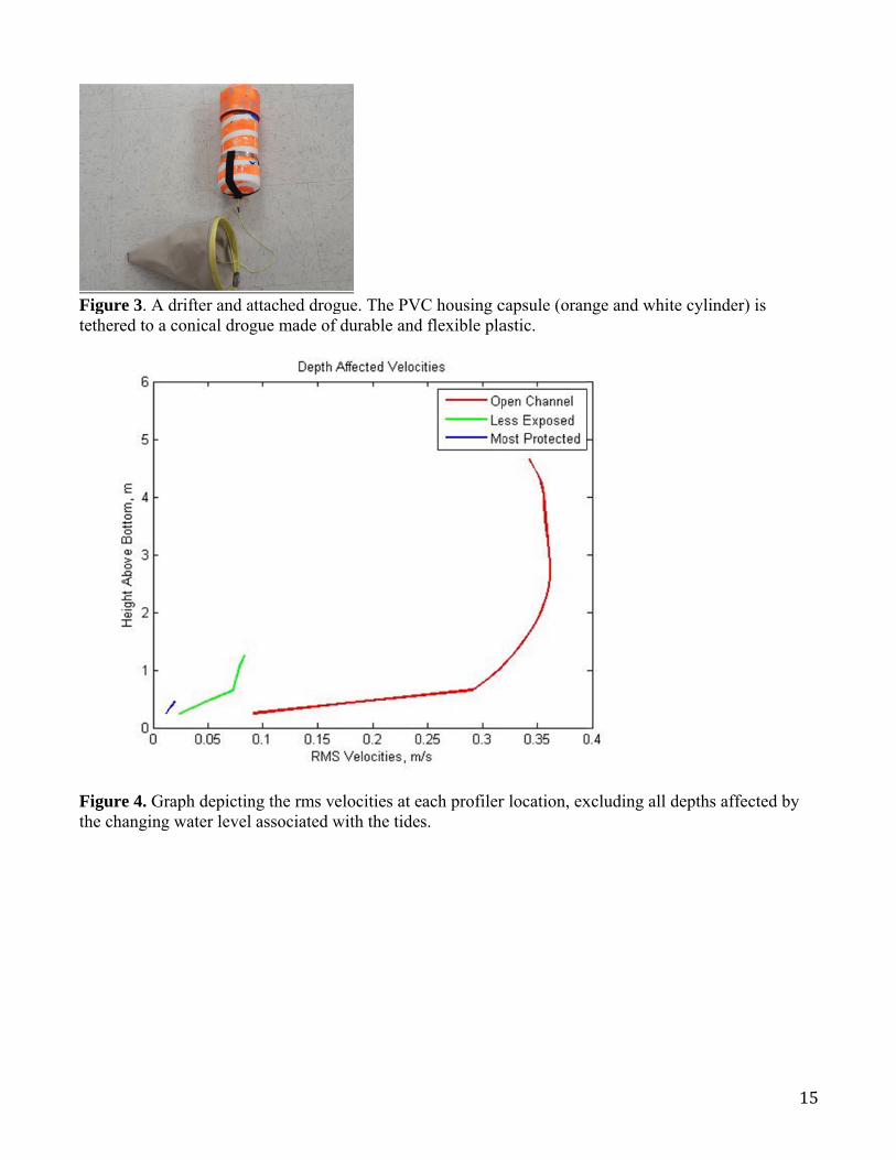
2.2 Drifters Complementing the current profiler data is a set of data gathered by drifters that were deployed throughout the marina for both a flood and ebb tide cycle. The drifters (Fig. 3) are comprised of a parachute drogue tethered to a hollow float that contained a 2-lbs weight to stabilize the float’s upright position and also included a Garmin Rino 520 or Garmin Rino 610 GPS device. The casing which houses the weight and GPS device is a cylindrical polyvinyl chloride (PVC) tube capped and sealed on both ends. The parachute drogue is conical in shape and functions by turning so that the open face is perpendicular to the orientation of the current flow. The current then pushes the drogue so that the drifter moves with the subsurface flow. GPS units were programmed to record their locations every two seconds as they moved around the marina. Deployments began for the ebb and flood tides (Oct 23 and Oct 3, respectively) at the outer edges of the marina in the path of the main channel; flood tide tracks

11

began on the eastern edge of the marina (closer to the ocean) while ebb tide tracks began on the western edge of the marina (closer to inputs from Calico Creek and the Newport River). Deployments continued for ebb and flood tides in between docks and on the outer edges of Docks A and D. After GPS data was collected from all drifter deployments, plots of velocity versus time were generated for each track. Due to large variations in GPS measurements of velocity, plots of distance traveled per signal versus cumulative time between drifter signals were created. These plots were then smoothed using a cubic spline curve, and the velocities were plotted onto an image of the marina. Current profiler data were reviewed to determine if tidal fluctuations for dates of drifter deployments were similar to other dates or exhibited unusual patterns that may bias the observed spatial structure of drifters.

3. RESULTS

3.1 Current Profilers Current profiler data were examined to determine the root mean squared (rms) flow speed for each point at which a profiler was deployed, the mean flow speed of water in the marina over the entire length of the deployment, and maximum velocities of flow for flood and ebb tides (Table 2, Table 3). Rms velocities were calculated at each of the three profiler locations. To avoid biases in data resulting from the changing water height at different tidal cycles, the rms velocities were only taken for the minimum height of the water (Fig. 4). These heights varied at each profiler location, and there is an obvious change in water height between the deeper open channel location and the shallower most protected location. The rms velocities of each of the profiles were also calculated (Table 2). There is a much greater rms velocity for the open channel point, which is most exposed to the constant tidal fluctuations and inputs from the Newport River and Calico Creek. The rms velocity is approximately 5 times greater than the rms velocity at the less exposed point beneath Dock B. The rms velocity at the less exposed point is itself approximately 5 times greater than the rms velocity measured at the most protected location. This intensive slowing of currents farther south into the marina suggests that the basin geometry effects the slowing of the currents on a much greater scale than any effects of the floating docks. This can be seen especially clearly when considering the discrepancy in rms velocities between the two profiler locations that were both stationed beneath Dock B. The mean flow speed for the duration of the entire deployment was calculated by first taking the mean of each recorded current profile, meaning that the velocities were averaged at each 25 cm above the current profiler for each measurement taken. These averages were taken up to the point at which water height was affected by tidal variation, producing values for high tide that were nonexistent during low tides. This profile average was then averaged for all profiles at the open channel location (Fig. 5). The open channel location was utilized for this calculation because the current profiler remained fixed while the second profiler was moved partway through the study period from the less exposed location to the most protected location. The mean flow speed was determined to be approximately -0.002 ± 0.334 m/s in the along channel direction and -0.005 ± 0.051 m/s in the across channel direction. These negative values are closely aligned with a southwest orientation, which would be indicative of currents associated with flood tide as water moves in from the Newport River and Morehead City port towards Calico Creek. The

12

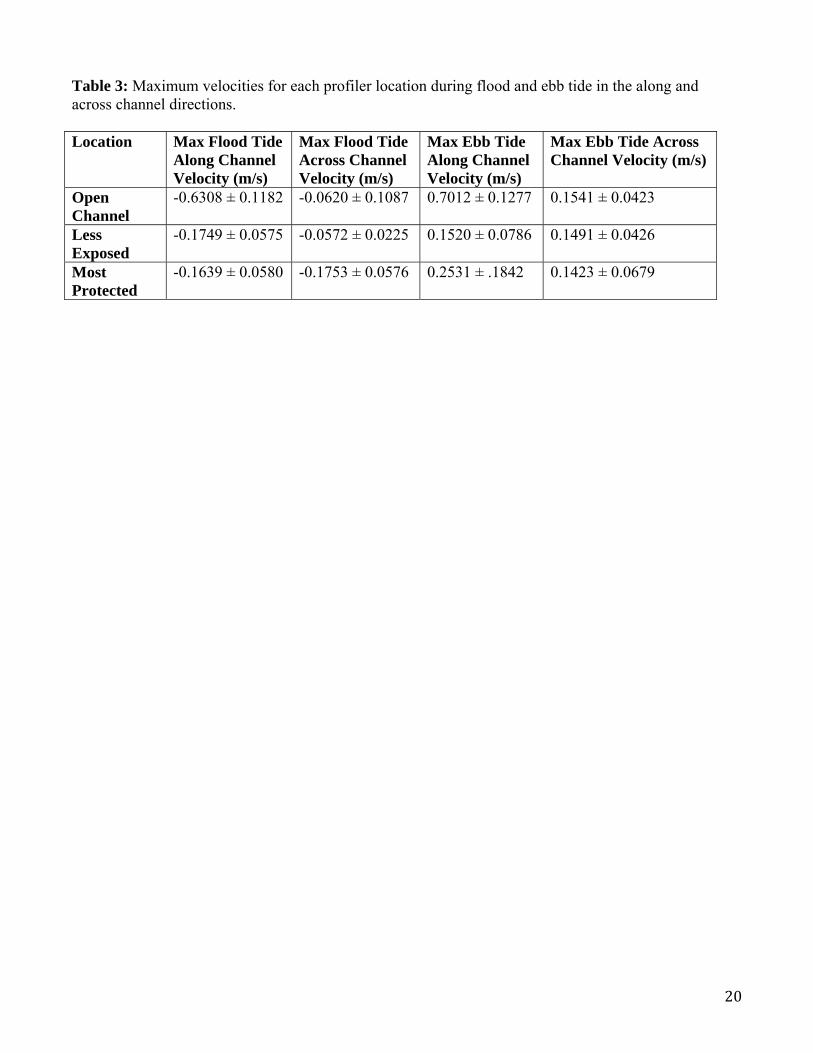
mean flow in this direction is indicative of stronger currents acting during flood tide in comparison with those during ebb tide. Stronger flood tide currents also indicate that they are likely to influence the circulation patterns more so than the currents prominent during ebb tide. The maximum flood and ebb tide velocities values were first calculated by taking the mean of the water column velocities for each current profile (Table 3). The maximum of these averages was then taken for both the along and across channel components of velocity to determine the maximum flood tide velocities. The minimum of these averages produced the maximum ebb tide velocities because ebb tide values were oriented such that they corresponded to the negative orientations for along and across channel velocities. Standard deviations were also calculated for each maximum and minimum average current velocity. These calculations were performed for each current profiler location. The date and time for each of these current velocities was also determined. The maximum average current velocities are found in the open channel, and these currents are approximately three to four times greater than the maximum currents found at either the less exposed or most protected locations. The differences in velocities between the less exposed and most protected locations are more peculiar and warrant further observation. While the current moving in the along channel direction (approximately East-West) at the less exposed location is almost three times greater than the across channel direction (approximately North-South) during the maximum flood tide, these two velocity components are almost equivalent during the maximum ebb tide. There exists a similar relationship for the maximum flood and ebb tides found at the most protected location, though the characteristics are reversed. In the case of the most protected location the maximum ebb tide velocity is almost doubled for the along channel component when compared with the across channel component. However, the two components are almost equivalent for the maximum flood tide velocity. While the values of maximum velocities for these components at the profiler locations can provide some information about the circulation patterns of the marina, it is necessary to incorporate data gathered by the drifters to develop a fuller conceptual spatial pattern.

3.2 Drifters Drifter deployments for both the ebb and flood tide measurements were graphed onto a satellite image of the MCYB (Fig. 9, 10). To ensure that the measurements of subsurface currents made by the drifters were not biased by the choice of deployment date, mean profile velocities from the open channel profiler data were compared with overall mean profile velocities. In this way, it was easier to discern if the particular lunar cycle or wind speed or other factors may have had a much larger influence than that which was anticipated. While over half of the velocity measurements made during flood tide measurements were greater than absolute mean velocity measurements (which avoided the impractical averaging of positive and negative measurements for this scenario), they did not vary appreciably or approach any of the calculated maximum velocity profiles. The absolute value of velocity measurements was determined to be 0.285 m/s, and the measurements made during the flood tide drifter deployments ranged from 0.2404 to 0.4886 m/s. Ebb tide deployments were made after the profilers had been removed from the basin, but recorded observations indicate that the ebb tide drifter deployments were made as the lunar cycle was waning and approaching a half moon. The subsurface measurements made by the drifters indicate that there is a large circulation cell occurring during flood tide, the momentum of which is compounded by the current patterns of ebb tide. During flood tide the currents originating from the Newport River move quickly through the main

13

channel, without moving laterally across the marina in any way near B, C, or Dock D. This water then entrains water that it passes by, drawing down the water level in the basin as water moves out from between and beneath the docks and also moves westward out of the basin towards Calico Creek. This movement necessitates some replacement of water, and this is accomplished by water moving along the west side of the marina near A and then spreading across the entire basin. Altogether, this movement of water creates a circulation pattern that rotates counterclockwise and flushes almost all of the basin. During ebb tide, currents move in from Calico creek eastward across the entire basin. Some currents continue unabated along the open channel, while others spread out across the basin. These currents slow down as they move into and across the basin but then are forced out on the eastward side of Dock D towards the open channel, where they are also flushed out of the basin. There are interesting current patterns near Dock A during flood tide where it appears that the southwest corner of the basin is unaffected in terms of flushing, but the currents moving past the more stagnant water are rotated and create a small eddy which remains relatively still in the isolated corner of the marina.

4. DISCUSSION The deployment of current profilers served to help provide information about how currents move throughout the basin over time, while the drifter deployments helped to develop a spatial scale at which an observer could determine how the entire body of water moves throughout the basin. According to data analysis and calculations of rms flow and the drifter patterns, it is apparent that the basin is relatively well flushed. This flushing occurs well within 12 hours for the slowest moving water volumes in the marina, the time required for two tidal cycles. In a single tidal cycle lasting 6 hours it is possible for a volume of water to enter the basin from the Newport River and move along the channel and around the entire basin before being flushed out towards Calico Creek. The same can be said for the ebb tide wherein a volume of water can be pushed across the entire basin to at least the other side of Dock D. Should the volume of water not be flushed within the ebb tide cycle, then it will likely be flushed out of the basin during the flood tide. The mean residual flow moving in a direction indicative of flood tide helps to assert an assumption that the flood tide is contributing to the currents encountered during ebb tide. This can be seen especially clearly at the less exposed profiler location, where the along and across channel velocities are slower than those reported during flood tide. This can be thought of as a volume of water being flushed out towards Calico Creek meeting another volume of water originating from Calico Creek and slowing down the volume as they are moving in opposite directions. The summary of this research indicates that the basin is well flushed, the docks have a negligible impact on the currents that move throughout the marina, and it is the geometry of the basin that dictates the speed of the currents. The speed of the currents then dictates the sediment size composition, faster flows seen in the channel matched with qualitative samples of a sandier bottom seen during the open channel profiler deployment. The slower currents within the marina ensure that much finer sediments will settle throughout the basin, also seen qualitatively during the under dock drifter deployments. The currents can therefore impact larger areas of study outside of those brought up in this study.

F

F

Fh

Figures and

Figure 1. Curr

Figure 2. Anhead of the in

d Tables

rent Profiler

n Aquadopp nstrument (r

Locations in

Current Proright).

n the Moreh

ofiler mounte

head City Ya

ed upon a ba

acht Basin.

ase after retriieval. The seensors are at

14

t the

Ft

Ft

Figure 3. A tethered to a

Figure 4. Grthe changing

drifter and aconical drog

raph depicting water level

attached droggue made of

ng the rms veassociated w

gue. The PVf durable and

elocities at ewith the tide

VC housing cd flexible pla

each profileres.

capsule (oranastic.

r location, ex

nge and whit

xcluding all

te cylinder)

depths affec

15

is

cted by

FS

Fv

Figure 5. GrStandard dev

Figure 6. Grvelocities for

raph depictinviation error

raph depictinr the open ch

ng mean resibars are also

ng velocitieshannel locati

idual velocito included.

s in the alongion.

ties for the op

g channel (X

pen channel

X, top) and ac

l profile at ea

cross channe

ach depth lo

el (Y, bottom

16

ocation.

m)

FvFigure 7. Grvelocities for

raph depictinr the less exp

ng velocitiesposed locatio

s in the alongon.

g channel (XX, top) and accross channe

el (Y, bottom

17

m)

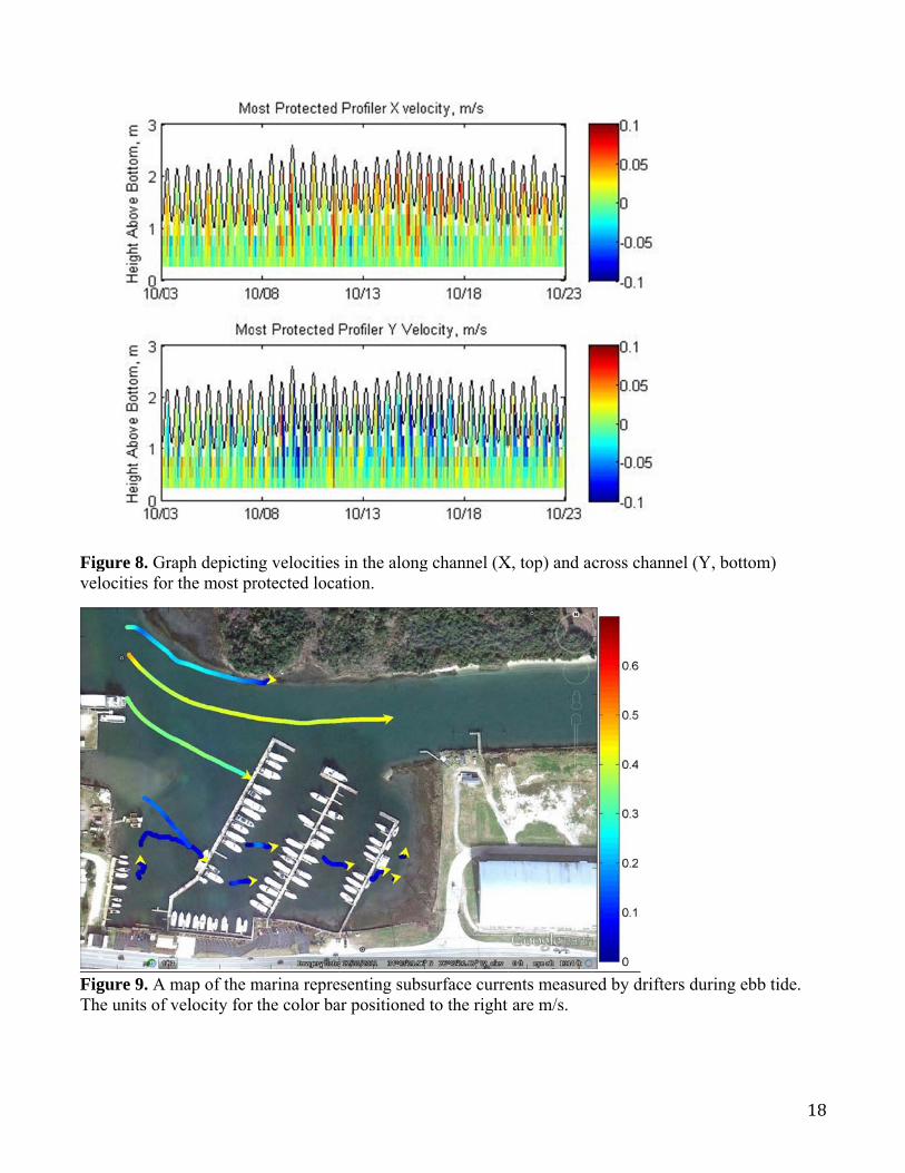
Fv

FT

Figure 8. Grvelocities for

Figure 9. A The units of

raph depictinr the most pr

map of the mvelocity for

ng velocitiesrotected loca

marina reprethe color ba

s in the alongation.

esenting subsar positioned

g channel (X

surface curred to the right

X, top) and ac

ents measure are m/s.

cross channe

ed by drifter

el (Y, bottom

rs during ebb

18

m)

b tide.

Fu

TLOLM TbwL

OCLEMP

Figure 10. Munits of the v

Table 1: GPLocation Open ChannLess ExposeMost Protec

Table 2: Velbecause the mwere deployeLocation

Open Channel Less Exposed Most Protected

Map of the mvelocity for t

S coordinateL

nel 3ed 3cted 3

locities recomean along ed.

RMS Ve 0.3337

0.0672

0.0169

marina showithe color bar

es and deploLatitude 34°43'21.9434°43'20.4134°43'18.30

rded for eacand across c

elocity (m/s)

ing subsurfacr on the right

oyment perio

"N "N "N

h profiler lochannel veloc

) MeanVeloc-0.00

N/A

N/A

ce currents rt of the imag

ods for each Longitude76°42'14.2276°42'14.8176°42'16.18

cation. N/A cities were i

n Along Chcity (m/s)

077 ± 0.0752

recorded by ge are m/s.

current prof

2"W 1"W 8"W

values are pinfluenced by

annel

2

drifters duri

filer. Deploymen9/24 – 10/29/24 – 10/310/3 – 10/2

provided for y the time du

Mean AcVelocity-0.0038 ±

N/A

N/A

ing flood tide

nt Period 23 3 23

two of the luring which

cross Channy (m/s) ± 0.0380

19

e. The

ocations h they

nel

20

Table 3: Maximum velocities for each profiler location during flood and ebb tide in the along and across channel directions. Location Max Flood Tide

Along Channel Velocity (m/s)

Max Flood Tide Across Channel Velocity (m/s)

Max Ebb Tide Along Channel Velocity (m/s)

Max Ebb Tide Across Channel Velocity (m/s)

Open Channel

-0.6308 ± 0.1182 -0.0620 ± 0.1087 0.7012 ± 0.1277 0.1541 ± 0.0423

Less Exposed

-0.1749 ± 0.0575 -0.0572 ± 0.0225 0.1520 ± 0.0786 0.1491 ± 0.0426

Most Protected

-0.1639 ± 0.0580 -0.1753 ± 0.0576 0.2531 ± .1842 0.1423 ± 0.0679

21

Chapter 2: Total Suspended Solids, Chlorophyll-a and Nutrients

1. INTRODUCTION

Water quality is important because it can provide an estimate of the condition of an aquatic ecosystem. In order to properly evaluate the water quality of a body of water and provide information to those who manage waterways, the spatial-temporal distribution of chlorophyll a, total suspended solids, and nutrients must first be assessed (Xu et al., 2012). As populations in coastal areas continue to grow, pressure from development is extending to riverine, estuarine, and coastal habitats (Peierls et al., 1991). This may have negative impacts on these ecosystems in the form of biodiversity loss, harmful algal blooms, hypoxia, and disease from pathogens and cyanobacterial toxins (Huisman et al., 2005). Eutrophication due to excessive nutrient-loading can affect nutrient cycling and lower water quality (Paerl, 1997). The main contributors are likely nonpoint sources where pollutants, such as gas and petroleum products, pesticides, and fertilizers, are scoured from the earth’s surface in the form of storm runoff (Sliva et al., 2001). Recreational water quality programs monitor water quality by noting levels of certain indicator bacteria such as total coliforms, fecal coliforms, and enterococci in order to help protect public health from risk of illness (Noble et al., 2003; NCDENR, 2013). Maintaining good water quality is necessary not only for the organisms that live in aquatic habitats, but also for the people that use it for drinking, recreation or fisheries management purposes, but also for the organisms.

One way to obtain a relative level of water quality is by measuring levels of chlorophyll a, total suspended solids, and nutrients and comparing these to other waterways and standards created as a benchmark of the levels of nutrient, chlorophyll-a and TSS that are expected and appropriate within a system to obtain an estimate of water quality. Chlorophyll-a allows one to gauge phytoplankton biomass and relative nutrient abundance (Wang et al., 2013). Chlorophyll-a concentrations can also be used to conclude a water body’s trophic status by evaluating its productive state (ibid). Chlorophyll-a serves as a useful indicator of water quality in water body management practices because it is rather easy to sample and measure (ibid).

Total suspended solids (TSS) are classified as a pollutant by the U.S. Clean Water Act (ibid). TSS has the ability to reduce water quality by clouding the water and consequently limiting light penetration and inhibiting photosynthesis of aquatic macrophytes (ibid). Sedimentation can also adversely affect aquatic life if suspended matter settles in excessive amounts and covers important habitat for marine organisms (ibid). Also, sometimes when individual particles are small (<63μm) they can carry harmful or toxic substances (ibid). This can be harmful for aquatic ecosystems as these suspended particles are transported and settle (ibid). Bio-magnification of chemical pollutants as particles transfer from filter feeders to larger consumers can also be a problem (ibid).

Phosphorus has long been thought to play a central role in controlling freshwater primary production and algal blooms (Likens, 1972; Paerl, 1988) with P input restrictions having been implemented since the 1960s to slow eutrophication rates (Schindler, 1977). Nitrogen commonly regulates primary production and phytoplankton biomass in estuarine and coastal waters (Nixon, 1992)

22

but anthropogenic nitrogen loading has increased in recent years and is now a large catalyst for coastal eutrophication (Paerl, 1987). In the end, the composition and concentration of nutrients will depend on how the watershed has been altered by agricultural and industrial activities (ibid).

The objective of this study was to assess the parameters commonly associated with water quality which includes chlorophyll-a, total suspended solids, and nutrients, in order to determine the relative water quality of the Morehead City Yacht Basin. This is important for the purposes of this study overall because our goal is to determine whether or not the activities occurring in the Morehead City Yacht Basin are responsible for greater environmental effects than those that would occur naturally, including a reduction in water quality. The null hypothesis being posed is that the yacht basin does not differ in water quality from nearby waters surrounding the marina. The conclusions reached in this study could help determine the impacts of yacht basins on the surrounding environment while also guiding management practices on how to best mitigate anthropogenic impacts.

2. METHODS

2.1 Field Sampling This study assessed the water quality of eighteen water samples collected from five different

locations within the Morehead City Yacht Basin in Morehead City, NC over a total of four days, one in September and three in October 2013. Our sample days involved traveling to the yacht basin to take water samples from five locations (Fig. 1), with sites 1-3 being sampled off the dock while 4 and 5 were accessed by boat. Samples were collected at high tide on day 1, low tide on day 2, at high tide and during a storm on day 3, and high tide on day 4. All samples were taken at approximately noon.

Samples were taken 1 m above the bottom using a Van Dorn water sampler. The Van Dorn was lowered with both ends open. The Van Dorn had a 1 m extension on it that hit the bottom first and allowed us to collect water from approximately 1 m above the bottom each time. When the Van Dorn reached the bottom, we dropped a messenger to shut both ends and entrap water inside. We then brought the Van Dorn to the surface and poured the sample into a 4L container using a funnel. The containers were rinsed with sample liquid before proceeding with pouring the entire sample. Each container was then filled with approximately 2L of liquid from its assigned sample site and then brought back to the lab.

2.2 Water Sample Analysis We prepared to quantify total suspended solids (TSS) by cleaning the filter rig with detergent

and deionized water and placing GF/F 47 mm diameter filters (0.7 microns pore size) on the filter rig wrinkle-side up. Each filter was flushed three times with 50 ml of deionized water and placed into tin boats within a foil pan covered with aluminum foil. We put this pan inside an oven (Thermo Electron

Corporation) at 60C, raised the temperature to 104C for 2.5 hours, and then lowered the oven

temperature to 60C. Once the filters cooled, they were removed from the oven and weighed (Mettler Toledo Classic Plus).

We then removed the rinsed and dried TSS filters from the oven and replaced them on the filter rig. 400 mL of sample water from each site was poured through an individual filtering device on the filter rig so that the suspended solids would accumulate on the filter. Two samples from each site were

23

filtered. After we filtered the samples, we put the filters back into their foil boats and placed them in the

oven once again. The oven’s temperature was increased to 104C for 2.5 hours to dry the filters. While the filters were drying, we filtered the sample water for nutrient analysis and froze the

filters for chlorophyll analysis. To do this the nutrient filter rig was cleaned with 3 rinses of deionized water and a 0.1 N hydrochloric acid rinse. We placed the 25 mm (0.7 microns pore size) filters atop the filter rig and then attached 30 mL magnetic graduated cylinders over top of the filters. 50 mL of water was filtered into 50mL vials and placed in the freezer for nutrient analysis. We did not replicate nutrient samples, but one replicate filter for each sample site was procured for chlorophyll analysis. The 25 mm filters were folded in half, dried with paper towels, and wrapped in tin foil and labeled before being placed in the freezer.

To assess chlorophyll a concentration in our water samples, we first kept the chlorophyll filters in the freezer for 24 hours. After this, we took them out, let them thaw, then ground them in an acetone solution in order to release their pigments. The grinding process took place under subdued lighting. Each filter was placed in a glass vial and filled with 3 mL of 90% acetone. We then ground the filter into a fine slurry using a grinder (Arrow Engineering CO., INC). The filter and acetone mixture was then decanted into a 15mL vial. The glass vial was rinsed with acetone and poured into the 15mL vial in order to ensure that all of the filter material was removed. We then filled capped the 15mL vial with 90% acetone up to the 10mL mark. Each sample was processed similarly and the set of samples were placed in the freezer overnight.

To complete quantification of TSS, the TSS filters were weighed a second time once they had cooled after being in the oven for 2.5 hours at 104°C. The new weight was noted and the difference was indicative of the weight of the suspended solids in the filtered water. The chlorophyll samples were also ready to be processed after 24 hours in the freezer. The tubes taken out of the freezer were shaken before placing them in the centrifuge (HermleLabnet) for 10 minutes at 6000 rpm. Then the fluorometer (Turner Designs Trilogy) was calibrated using a solid standard and an acetone blank. We filtered approximately 3ml of each of sample through a 25mm filter (0.7 micron pore size) using a syringe into a cuvette, being careful not to disturb the material that has been centrifuged to the sides. Cuvettes were then inserted into the fluorometer in order to measure the fluorescence of the sample.

3. RESULTS

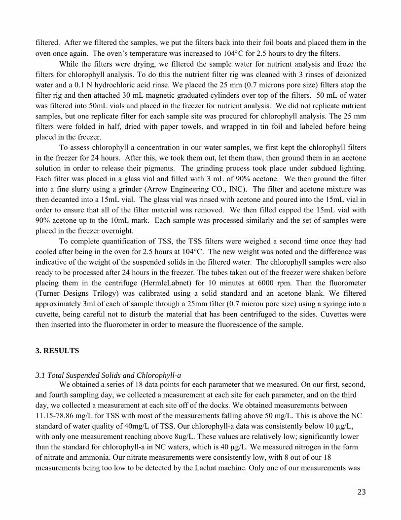
3.1 Total Suspended Solids and Chlorophyll-a We obtained a series of 18 data points for each parameter that we measured. On our first, second, and fourth sampling day, we collected a measurement at each site for each parameter, and on the third day, we collected a measurement at each site off of the docks. We obtained measurements between 11.15-78.86 mg/L for TSS with most of the measurements falling above 50 mg/L. This is above the NC standard of water quality of 40mg/L of TSS. Our chlorophyll-a data was consistently below 10 µg/L, with only one measurement reaching above 8ug/L. These values are relatively low; significantly lower than the standard for chlorophyll-a in NC waters, which is 40 µg/L. We measured nitrogen in the form of nitrate and ammonia. Our nitrate measurements were consistently low, with 8 out of our 18 measurements being too low to be detected by the Lachat machine. Only one of our measurements was

24

above 5 µg/L. Our ammonia levels ranged from 16.9-64.1 µg/L. These values, and the values found for nitrate concentrations are at or below the levels found in the Newport River and Calico Creek waterways (Kirby-Smith). Using separate 1-way ANOVA tests and Tukey’s HSD post-hoc multiple comparisons, we assessed whether TSS, chlorophyll-a, nitrate, ammonia, and phosphate concentrations differed between sites and over time throughout the course of our study. When analyses were conducted with data collected during the storm, only sites 1, 2, and 3 were included because sites 4 and 5 were inaccessible on that date. When data was analyzed without the storm measurements, all five sites were used. In these analyses, only data collected on the 1st, 2nd, and 4th sampling days were included. Our analysis of Total Suspended Solids (TSS) did not indicate significant differences within the basin, either between sites (p = 0.485; Fig. 2) or between sampling times (p = 0.202; Fig. 3).

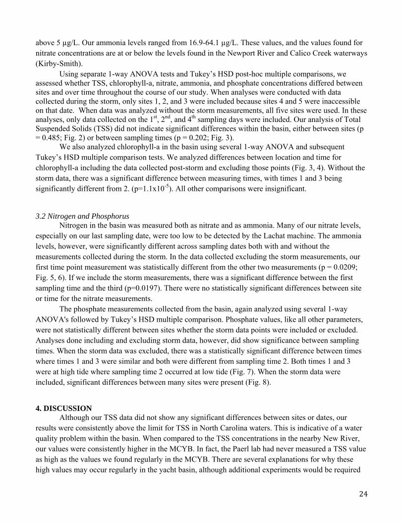
We also analyzed chlorophyll-a in the basin using several 1-way ANOVA and subsequent Tukey’s HSD multiple comparison tests. We analyzed differences between location and time for chlorophyll-a including the data collected post-storm and excluding those points (Fig. 3, 4). Without the storm data, there was a significant difference between measuring times, with times 1 and 3 being significantly different from 2. (p=1.1x10-5). All other comparisons were insignificant.

3.2 Nitrogen and Phosphorus Nitrogen in the basin was measured both as nitrate and as ammonia. Many of our nitrate levels,

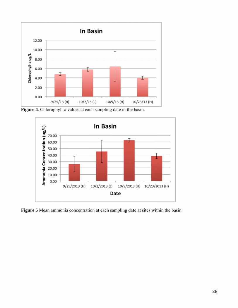
especially on our last sampling date, were too low to be detected by the Lachat machine. The ammonia levels, however, were significantly different across sampling dates both with and without the measurements collected during the storm. In the data collected excluding the storm measurements, our first time point measurement was statistically different from the other two measurements (p = 0.0209; Fig. 5, 6). If we include the storm measurements, there was a significant difference between the first sampling time and the third (p=0.0197). There were no statistically significant differences between site or time for the nitrate measurements.

The phosphate measurements collected from the basin, again analyzed using several 1-way ANOVA's followed by Tukey’s HSD multiple comparison. Phosphate values, like all other parameters, were not statistically different between sites whether the storm data points were included or excluded. Analyses done including and excluding storm data, however, did show significance between sampling times. When the storm data was excluded, there was a statistically significant difference between times where times 1 and 3 were similar and both were different from sampling time 2. Both times 1 and 3 were at high tide where sampling time 2 occurred at low tide (Fig. 7). When the storm data were included, significant differences between many sites were present (Fig. 8).

4. DISCUSSION Although our TSS data did not show any significant differences between sites or dates, our

results were consistently above the limit for TSS in North Carolina waters. This is indicative of a water quality problem within the basin. When compared to the TSS concentrations in the nearby New River, our values were consistently higher in the MCYB. In fact, the Paerl lab had never measured a TSS value as high as the values we found regularly in the MCYB. There are several explanations for why these high values may occur regularly in the yacht basin, although additional experiments would be required

25

in order to ascertain which mechanisms are active in the yacht basin. One explanation is that the yacht basin is a fairly enclosed geographical feature, and the combination of its fairly shallow depths paired with low current speeds may increase the accumulation and resuspension of finer sediments at the within the basin (Chapter 2, 12; Fig. 4; Fig. 8). There is also likely sediment input from nearby Calico Creek that contributes to the overall sediment load, and organic matter input from organisms attached to the floating docks (i.e. feces and pseudofeces or organisms that had become detached from the docks). The marina itself likely is only responsible for causing increased boat traffic as well as providing hard substrate for the attached organisms, and may contribute to increased levels of TSS through those mechanisms.

The levels of chlorophyll-a in the basin were consistently low; well below the state standard of 40 µg/L. These chlorophyll levels are also comparable with the levels of chlorophyll-a found by the Paerl lab in Pamlico Sound. Pamlico Sound is a water body that is known to have very good water quality, indicating that the MCYB is likely not experiencing problems with eutrophication or excessive algal production. The differences in chl-a across sampling times did coincide with tide; chlorophyll-a was higher during low tide than high tide. This general pattern was noticeable in our nutrient data as well, even where the differences were not large enough to be statistically significant, suggesting that tidal phase may influence nutrient availability and, therefore, phytoplankton growth.

The nitrate and ammonia levels found in the basin were similar to the usual levels found in the Newport River Estuary area (Kirby-Smith & Costlow, 1989). No significant differences in either nitrate or ammonia were found across sites. This likely indicates that the presence of the marina does not have a strong impact on nutrient levels in the area; they remain consistently similar to established normal levels. Our ammonia measurements did differ across time, both with the inclusion of storm data and without it, and was higher at low tide than at high tide. We did not have enough time points to draw conclusions from this difference, although it may be due to tidal influence and other natural processes such as the input of freshwater from nearby creeks.

Phosphate, similarly, was not significantly different between sites. Levels were also relatively low within the basin, indicating that the phosphate levels in the basin are not largely impacted by the presence of the marina. The phosphate levels did differ between sampling times, again being higher at low tide than high, whether the storm data points were included or excluded. When the storm data points are included, the phosphate levels during the storm were comparable with the levels at our low tide sampling date. Again, we did not sample at enough time points to be able to determine whether these differences are correlated with tidal stage, although this could be reasonably expected to play a role in the flushing and addition of nutrients to the basin by assisting in the transport of nutrients in and out of the basin. The lower levels of nutrients at high tide seem reasonable, as this may be when a large amount of oligotrophic seawater is carried into the basin. When the storm data is included in the analysis, there are still statistically significant differences between the sampling times, but the storm itself does not seem to largely increase phosphate levels in the basin.

Looking at these water quality parameters is helpful in assessing the overall impact of the yacht basin. Although the presence of the marina does not seem to be causing an extreme decrease in water quality in the basin, it is possible that some of the differences we encountered in our data are due to the presence of human activity in the area. Our TSS data especially shows an area where the marina may have an environmental impact through the suspension of sediments by boats and the input of organic

mrbmF

F004W

F

matter by serequire additbetter picturmanagementFigures and

Figure 1. W076"42.253')076"42.265')4 (N 34"43.4W 076"42.04

Figure 2. Me

essile organitional researe of the impt solutions to

d Tables

ater quality ) is located n) at the midp437' W 076"444') also in th

ean TSS val

sms on the rch. Certainpact the mao the marina

sampling sitnear a storm point of Dock42.373') in the channel b

ues found at

floating docnly, ongoing arina has on .

tes at the Modrain at the k B, site 3 (Nhe adjacent but closer to

t each sampl

cks, althoughmonitoringwater quali

orehead Citycorner of Do

N 34"43.355channel towBogue Soun

ling site.

h a certain ag of water qity, and wou

y Yacht Basiocks B and S

5' W 076"42wards Calico nd.

assessment oquality paramuld help pro

in. Site 1 (NS, site 2 (N 3.240') at the Creek, and

of this impameters woulovide more

N 34"43.264' 34"43.315' Wend of Docksite 5 (N 34"

26

act would ld give a effective

W W k B, site "43.380'

F

F

Figure 3. Th

Figure 3. Me

he mean conc

ean chloroph

centration of

hyll-a values

f TSS found

s at each sam

d in the MCY

mpling date a

YB at each sa

at the channe

ampling date

el sites.

e.

27

F

F

Figure 4. Ch

Figure 5 Me

hlorophyll-a

ean ammonia

values at ea

a concentrati

ach sampling

ion at each s

g date in the

sampling dat

basin.

te at sites wi

ithin the basiin.

28

F

F

Figure 6. Me

Figure 7. Me

ean ammoni

ean phospha

ia concentrat

ate concentra

tion at each

ation at each

sampling da

h sampling d

ate for chann

ate for chann

nel sites.

nel sites.

29

F

Figure 8. Me

ean phosphaate concentraation at eachh sampling date for basin

n sites.

30

31

Chapter 3: Microbial Activity

1. INTRODUCTION The importance of monitoring surrounding waters for the presence of harmful bacteria and

pathogens has increased as a result of increasing statistical knowledge of water-related deaths and increasing population density of coastal communities. In 2010, 39 percent of the United States’ human population lived near the coast, and this number is projected to increase another 8 percent by 2020 (NOAA, 2013). With high population densities near the ocean, the importance of finding water contamination in a timely manner is essential to the water-related health of the population. Human contact with fecal contamination either through skin contact or ingestion can cause gastrointestinal illness and other side effects (Fries et al., 2006). Measurements of indicator bacteria are used to calculate potential health risks to society (Shibata et al., 2004; USEPA, 2011) and to provide a basis for decisions toward recreational and commercial uses of water (USEPA, 2011).

Fecal indicator bacteria, such as Enterococcus and Escherichia (E. coli), are found in the gut of warm-blooded animals and are not normally found in open environments. These non-pathogenic bacteria are often used to indicate the presence of fecal contamination (Dufour & Ballentine, 1986). The presence of fecal contaminants in open marine environments may be attributable to wastewater discharge, direct discharge into waterways, or stormwater outfall. Studies show that urban stormwater runoff is a major non-point source of water contamination to surrounding waters (Selvakumar & Borst, 2006). Rainfall increases stormwater contamination through the rinsing of fecal contamination on land, such as animal feces, into the surrounding water. This output contains both contamination and indicator bacteria (Selvakumar & Borst, 2006). High levels of enterococci in recreational waters have been identified as a causal factor for gastrointestinal illnesses (Currieo et al., 2001; Fries et al., 2006). Other studies support the use of indicator bacteria for monitoring recreational waters, such as beaches and estuaries (Lipp et al., 2001; Desmarais et al., 2002; Boehm et al., 2004; Bare et al., 2013).

Currently, North Carolina has three classifications of tidal waters: SA (saltwaters satisfactory for commercial shellfishing and all other saltwater uses), SB (saltwaters intended for primary recreation), and SC (saltwaters protected for secondary recreation, fishing and and aquatic life). These tidal waters are categorized by their uses and have varying respective water quality standards. SA has the lowest set allowable bacteriological limit and SC has the highest allowable bacteriological limit (NCAC). To retain these classifications of tidal waters, managers are required to maintain fecal indicator bacteria levels so that they do not fall below set limits. These levels are set at 320 MPN per 100 mL for E. coli and 104 MPN per 100 mL for Enterococcus for single samples so that safe recreational water health may be preserved (NCAC).

There are many factors that affect the levels of fecal indicator bacteria. Documented laboratory studies show decreased microbial death due to predation or environmental exposure if bacteria are attached to particles (Davies & Bavor, 2000). Stenstrom (1989) found that Enterococcus has greater attachment rates to inorganic particles (56-77%) than E. coli (21-29 %). Another study found similar differences between the bacteria in attachment to inorganic particles in stormwater with Enterococcus (38-52%) having a greater attachment rate than E. coli (16-34%) (Characklis et al., 2005). Other factors such as visible light, salinity and water temperature affect microbial activity. However, increased salinity was observed to only have a toxic effect on E. coli compared to Enterococcus (Barcina et al.,

32

1990). Water temperature can also affect growth rates of bacteria. Studies have found supporting data that indicate low water temperatures are optimal for bacterial growth in water (Edberg et al., 2000; Faust et al., 1975).

McMahon (1989) suggested that while an individual marina may not impact the quality of the surrounding water bodies, the cumulative impact of several marinas may significantly degrade the surrounding marine environments. Potential impacts on the water system include increased turbidity, lower dissolved oxygen, increased nutrient and bacteria loading, and increased hydrocarbon loading (McAllister, 1996).

The overall goal of the microbiological study was to identify how a tidal-water marina with floating docks would affect the surrounding ecosystem by measuring surface particle suspension characteristics and the concentrations of selected fecal indicators in Morehead City Yacht Basin. We hypothesized that there would be a significant difference in total suspended solids and fecal indicator bacteria outside the marina versus inside the marina. Another goal was to see the effect of stormwater draining into the marina on the water bacteriological levels. These hypotheses were tested by taking and analyzing water samples from locations in the channel beside the marina and within the marina itself with one location at the stormwater pipe.

2. METHODS

2.1 Sampling Sites Water samples were collected on Sept 25, Oct 2, and Oct 23, 2013 at six locations within the Morehead City Yacht Basin (Fig. 1). Two high tide samplings occurred on Sept 25 and Oct 23 and a low tide sampling occurred on Oct 2. Site 1 was located on Dock S at the back of the yacht basin near a stormwater drain output. Site 2 was near a gasoline pump station on Dock B. Site 3 is at the end of Dock B near the channel. Sites 4 and 5 were located in the channels leading to the yacht basin. Site 6 was located in the corner of the yacht basin where the water depth became relatively shallow during low tides. Samples were taken 30 cm below the water surface in sterile Nalgene bottles. Two sets of water samples, one 250 mL and one 500 mL, were taken at each site. The smaller of the two water samples (250 mL) was used to test for total coliforms, E. coli, and Enterococcus and the other water sample (500 mL) was used to quantify total suspended solids. The water samples were placed in a cooler with ice packs to slow microbial activity and were transported immediately back to the lab and placed in a refrigerator.

2.2 Laboratory procedures Total coliforms and E. coli were enumerated using an IDEXX Colilert-18 test kit and

Enterococcus using an IDEXX Enterolert test kit. For each analysis, a 10 mL water sample was mixed with 90 mL of deionized water and the appropriate media. The solutions was transferred into a 51-well Quanti-Tray, sealed and incubated for 18 hours at 35°C and 41°C for E. coli and Enterococcus respectively. After incubation, the trays were examined under an ultraviolet light and fluorescing wells were counted. The most probable number (MPN) was determined for each sample by correlating the amount of fluorescent wells to the IDEXX 51-Well Quanti-Tray MPN table. Calculations were made to correct for the amount of water sampled by multiplying the MPN by 10 since only 10 mL of water of the 100 mL sample was used.

33

Along with testing for fecal indicator bacteria, measures of salinity and pH were taken from each 500 mL water sample once in the lab. To measure salinity, a digital refractometer model HI 96822 was used. Once calibrated, 2 drops of sample were placed on the well and the salinity was recorded. Wind velocity and water temperature were retrieved from a buoy station in Beaufort, NC (N 34.72’ W 76.67’). Rainfall data for 24, 48, and 72 hours were taken from NDBC Station CLKN7 (N 34.622’ W 76.525’).

To determine the total suspended solids within a 500 mL water sample, two 100 mL subsamples were taken after mixing and measured using a 100 mL graduated cylinder. Water was vacuum filtered through 0.7-micrometer pore-sized glass fiber filters. The filters were prepped prior to filtering by being placed in aluminum foil packets and stored at 105°C for 24 hours. After drying, the filter packets were weighed on an analytical balance capable of weighing to 0.001 g to determine pre-filtering mass. Deionized water was used to rinse off any particle residue from the filter funnel. After filtration, the filters were placed back into the oven at 105°C to dry. After 24 hours, the filter packets were taken out and weighed again to calculate the weight difference.

3. RESULTS

3.1 Fecal Indicator Bacteria Total coliforms, E. coli, and Enterococcus concentrations at each site were compared between the sampling days (Fig. 2, Fig. 3). One-way ANOVA showed total coliforms between sampling days were not significant (p=0.05). E. coli concentrations significantly decreased between days 1 and 3 (p=0.0334) and days 2 and 3 (p=0.0141) but were not significant between days 1 and 3. Total coliforms, E. coli and Enterococcus concentrations between sites showed no significant differences (Fig. 4, Fig. 5). To determine if the floating docks contributed to higher concentrations in bacteria, sites located within the marina (Site 1, 2, 6) were compared to the sites located along the channel of the yacht basin (sites 3, 4, 5). Bacterial concentrations within the marina did not significantly vary with the locations outside of the marina. For all sites and sampling days, Enterococcus showed no positive wells and the corresponding MPN was <10. 3.2 Total Suspended Solids Total suspended solid (TSS) concentrations from each site were compared among the three different sampling days (Fig. 6). TSS significantly increased on sampling days 1 and 2 with a p-value of 0.0299 but showed no significant difference between each site (Fig. 7). For each sampling day, fecal indicator bacteria concentrations were compared to TSS which showed no correlation to weak correlations (Table 1). All TSS levels were above the set US EPA standard of 20 mg per liter (NCDENR, 2007).

3.3 Rainfall, Salinity and Water temperature Other parameters were also observed at the Yacht Basin that could contribute to bacteria concentrations. Previous rainfall data were looked at 24, 48, and 72 hours prior to sampling date (Table 2). On sampling day 3 within 72 hours there was a total of 5.90 cm3 of rainfall. The average salinity for each sampling day remained consistent, ranging from 35.5-36.17 psu (Table 3). The average water temperature was taken for each sampling day, which ranged from 20-24°C (Table 4).

34

4. DISCUSSION The goal of this study was to examine the biological characteristics and surface suspended solids

of water within the Morehead City Yacht Basin in order to understand the effects of marinas on biological water quality. We found few significant correlations in fecal indicator bacteria and total suspended solids within the marina compared to tide specification, sampling location, and stormwater outfall.

4.1 Fecal Indicator Bacteria The significant decrease in concentration levels between high tide sampling days 1 and 3 can be due

to different sampling times. During flood tide, water coming from the ocean through Beaufort Inlet and into the yacht basin will have lower bacterial concentrations than during ebb tide. Ebb tide will have higher concentrations of total coliforms and E. coli due to more input from land runoff (Selvakumar & Borst, 2006). If sampling occurred on Sept 25 slightly prior to high tide, bacterial concentrations could be higher due to less dilution than on Oct 25, resulting in a significant difference between sampling days. The significant decrease in concentrations between low tide sampling and high tide sampling on days 2 and 3 is due to increased drainage into the yacht basin from land due to low tide bringing in higher bacterial concentrations (Selvakumar & Borst, 2006).

The US EPA water quality standard for E. coli is 320 MPN/100 mL. Out of all six sampling sites during the three sampling days, only one site on day 2 had a MPN/100 mL higher than the set standard. This was site 1 on low tide, which was directly next to the stormwater drain. For all sampling sites and days Enterococcus concentrations were less than 10 MPN/100 mL. These levels were well below the US EPA set standard of 104 MPN/100 mL for Enterococcus (NCAC). Therefore, there was no indication of inputs or impacts from the marina to introduce Enterococci into the water. Contrary to Bare’s study, the concentrations from this study between each sampling site and sites located inside the marina versus sites outside the marina were not significant during a one-way ANOVA test. The impact of the floating docks did not show a significant effect on the flow rates to increase concentrations within the marina (Chapter 1).

4.2 Total Suspended Solids TSS significantly increased between low tide and high tide on days 1 and 2. This can be due to

shallower water on day 2 and wind velocity increasing suspended solids due to re-suspension from bottom sediments (Schoellhamer, 1996). Since bacteria have been shown to attach to particles, an increase in suspended solids would result in higher bacterial concentrations (Stenstrom, 1989; Barcina et al., 1990; Davies & Bavor, 2000; Characklis et al., 2005; Fries et al., 2006). However, there was no correlation between concentrations and TSS for all three sampling days. This could be due to lower TSS values seen within the yacht basin compared to outside the basin and attachment from bacteria could occur at relatively higher TSS values than were present.

4.3 Other Parameters Examined Few data points and replicates reduce the accuracy of rainfall amount, salinity level, and water

temperature comparisons to fecal indicator bacteria concentrations. Additional data, including water sampling after storms and year-round sampling, would provide information about the effects of increased amount of rainfall and stormwater outfall and different levels of water temperature. Data from

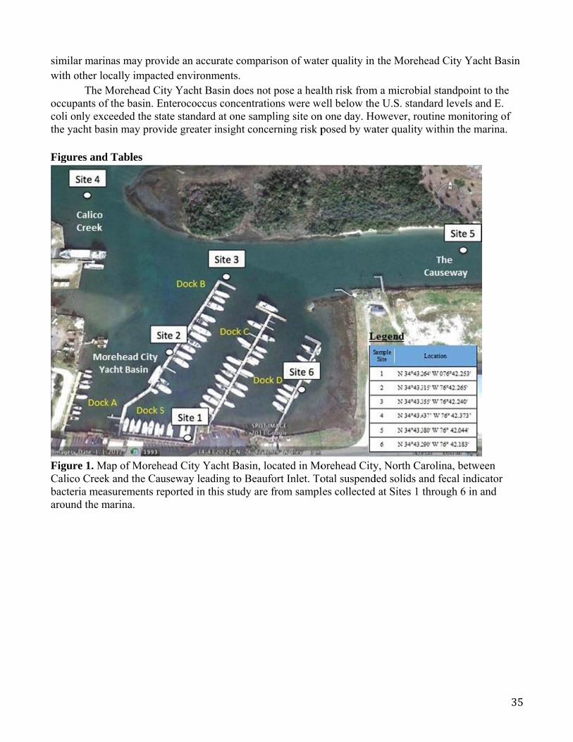
sw oct F

FCba

similar marinwith other lo

The Moccupants ofcoli only excthe yacht bas

Figures and

Figure 1. MaCalico Creekbacteria meaaround the m

nas may provocally impactMorehead Cf the basin. Eceeded the stsin may prov

d Tables

ap of Morehk and the Cauasurements remarina.

vide an accuted environmity Yacht Ba

Enterococcustate standardvide greater

head City Yauseway leadeported in th

urate comparments. asin does nots concentratid at one sampinsight conc

acht Basin, loding to Beauhis study are

rison of wate

t pose a healions were wepling site oncerning risk p

ocated in Mofort Inlet. Tofrom sampl

er quality in

lth risk fromell below the

n one day. Hoposed by wa

orehead Cityotal suspendles collected

the Morehe

m a microbiale U.S. standowever, rout

ater quality w

y, North Carded solids and at Sites 1 th

ad City Yac

l standpoint dard levels antine monitor

within the m

rolina, betwend fecal indichrough 6 in a

35

cht Basin

to the nd E. ring of arina.

een cator and

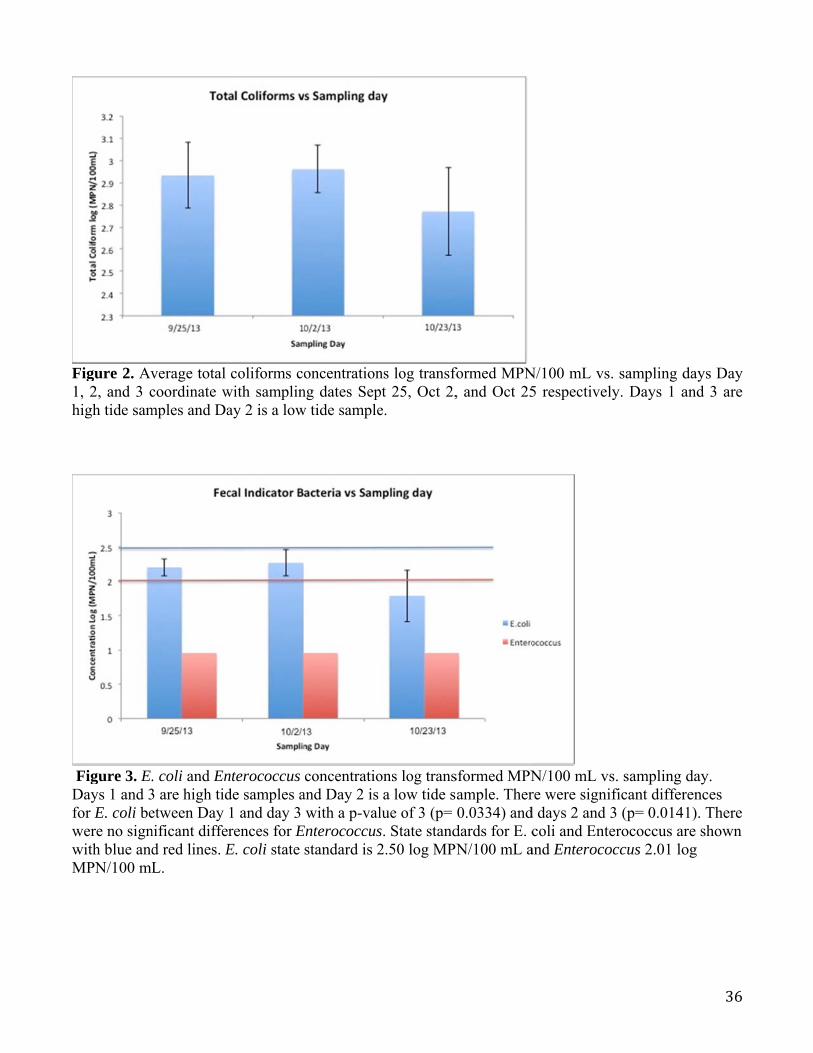
F1h

DfwwM

Figure 2. Av1, 2, and 3 chigh tide sam

Figure 3. E.Days 1 and 3for E. coli bewere no signwith blue andMPN/100 mL

verage total coordinate wmples and Da

. coli and En3 are high tidetween Day nificant diffed red lines. EL.

coliforms cowith samplinay 2 is a low

nterococcus de samples a1 and day 3 rences for EE. coli state

oncentrationng dates Sepw tide sample

concentratioand Day 2 is with a p-val

Enterococcusstandard is 2

ns log transfopt 25, Oct 2,e.

ons log transa low tide s

lue of 3 (p= s. State stand2.50 log MPN

formed MPN, and Oct 25

sformed MPNample. Ther0.0334) and

dards for E. cN/100 mL a

N/100 mL vs5 respectivel

N/100 mL vre were signid days 2 and coli and Ent

and Enteroco

s. sampling dly. Days 1 a

vs. sampling ificant differ3 (p= 0.014

terococcus aroccus 2.01 lo

36

days Day and 3 are

day. rences 1). There re shown og

Fs

FTsl

Figure 4. Avsignificant di

Figure 5. E. There was nostandards forlog MPN/100

verage total ifferences be

coli and Ento significantr E. coli and 0 mL and En

coliforms coetween site l

terococcus ct difference bEnterococcu

nterococcus

oncentrationlocations (p

concentrationbetween siteus are shown2.01 log MP

ns log transfo> 0.05)

ns log transfe locations fon with blue aPN/100 mL.

formed MPN

formed MPNor either fecaand red lines

N/100 mL vs

N/100 mL vsal indicator bs. E. coli stat

s. site. There

s. site locatiobacteria. State standard i

37

e were no

ons. ate is 2.50

Fsa

Fe

Figure 6. Avsample. TSSall sampling

Figure 7. Averror, all site

verage TSS v showed a sidays had lev

verage TSS es had levels

vs. samplingignificant invels of TSS

vs. site locaof TSS high

g day. Days crease on sahigher than

ation. TSS shher than the

1 and 3 are hampling daysthe set EPA

howed no siset EPA stan

high tide sams 1 and 2 (p=standard of

ignificant difndard of 20 m

mples and D=0.0299). Wf 20 mg per l

fference betwmg per liter.

ay 2 is a lowWithin error r

liter.

ween each s.

38

w tide region,

site. With

39

Table 1. Bacterial Concentration vs. Total Suspended Solids Pearson coefficient R2 values.

Day Total Coliforms E. coli

1 0.01141 0.02582

2 0.35464 0.27286

3 0.16699 0.37415

Table 2. Cumulative Rainfall over 72 hour period prior to sampling day.

Day 24 hours 48 hours 72 hours

1 0 0 0

2 0 0 0

3 5.41 cm3 5.90 cm3 0

Table 3. Average salinity. All water samples had approx. 35 or 36 psu.

Day Average Salinity Tide

1 36.17 psu High

2 34.83 psu Low

3 35.50 psu High

Table 4. Average Water Temperature. Day 1 through 3 data had decreasing water temperatures respectively.

Day Average Water Temperature (Degrees Celsius)

1 23.3

2 22.8

3 20.6

40

Chapter 4: Light Attenuation

1. INTRODUCTION Marsh plants and submerged aquatic vegetation (SAV) provide a nursery habitat and source of primary production for a vast amount of shellfish, mollusks, birds, mammals, and fish (Weinstein 1996). Both marsh grass and sea grass species have evolved to photoacclimate to varying amounts of incident light at different latitudes but struggle to survive without at least 15 – 25% incident light (Dennison et al., 1993, Kenworthy and Haunert 1991). The amount of light reaching the SAV from the surface based on the optical properties of the water can be calculated using the Beer-Lambert law and then taken as a percent of surface incident light. The two most abundant species of sea grass found along the shores of North Carolina are near the limits of their preferred ranges. The more northern species Zostera marina generally inhabits sandy bottoms up to 6 meters in depth with a minimum of 15 - 18.6% incident light (Io) (Burdick and Short 1999, Dennison, 1993). The more tropical species, Halodule wrightii, is found in shallower depths of up to 1.9 meters with a minimum of 13 - 17.4% Io (Shaefer and Robinson 2001, Dennison et al., 1993). These minimum incident light requirements were calculated using secchi disk methods and by recording the median values of the intersection point of the light extinction curves with the maximum depth of SAV survival curves during the growing months of each species (Dennison et al., 1993). Light limitation from the shading effects of marinas may lead to physiological stress possibly resulting in diminished growth, increased shoot mortality, and limited depth distribution (Kenworthy 1996).

In order to determine the shading effects of floating docks on the ecosystem we measured the level of incident light reaching the bottom and the rate of light attenuation in the water column. These measurements were conducted beneath, between, and away from docks in the marina and compared with a control completely removed from the water column.

2. METHODS

2.1 Light Available for SAV To measure light intensity on the basin floor of the Morehead City Yacht Basin twelve HOBO

Pendant® Temperature/Light Data Loggers were deployed. These sensors were attached individually to cinderblocks (Fig. 1, Fig. 2) using Zipties and anchored to a piling close by in order to prevent loss. The GPS coordinates where each sensor was placed were taken and the anchor line was tied to selected pilings. A boat and dive team were used to deploy the sensors for the four light sensors deployed between the docks. Six other sensors lines were lowered from the dock and left for divers to place underneath the dock. One sensor was lowered from a boat away from the marina’s floating docks and closer towards the fixed dock on the west side of the basin to keep it away from most shading effects. A control light sensor was then used to estimate incident light and was attached to a brick using the same method and was placed on the roof of a pump house at the University of North Carolina Chapel Hill’s Institute of Marine Sciences.

Each sensor then recorded the light intensity at constant five-minute intervals and was left in place for a period of three weeks. Data collection began on September 26, 2013 and the light sensors were removed from the marina on October 22 (Fig. 3). To show the viability of SAV in the basin, we

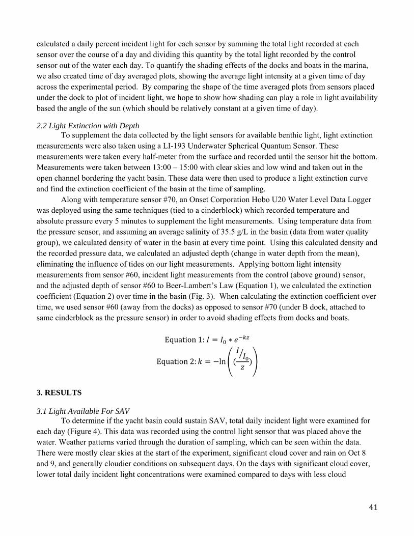
41

calculated a daily percent incident light for each sensor by summing the total light recorded at each sensor over the course of a day and dividing this quantity by the total light recorded by the control sensor out of the water each day. To quantify the shading effects of the docks and boats in the marina, we also created time of day averaged plots, showing the average light intensity at a given time of day across the experimental period. By comparing the shape of the time averaged plots from sensors placed under the dock to plot of incident light, we hope to show how shading can play a role in light availability based the angle of the sun (which should be relatively constant at a given time of day).

2.2 Light Extinction with Depth To supplement the data collected by the light sensors for available benthic light, light extinction measurements were also taken using a LI-193 Underwater Spherical Quantum Sensor. These measurements were taken every half-meter from the surface and recorded until the sensor hit the bottom. Measurements were taken between 13:00 – 15:00 with clear skies and low wind and taken out in the open channel bordering the yacht basin. These data were then used to produce a light extinction curve and find the extinction coefficient of the basin at the time of sampling. Along with temperature sensor #70, an Onset Corporation Hobo U20 Water Level Data Logger was deployed using the same techniques (tied to a cinderblock) which recorded temperature and absolute pressure every 5 minutes to supplement the light measurements. Using temperature data from the pressure sensor, and assuming an average salinity of 35.5 g/L in the basin (data from water quality group), we calculated density of water in the basin at every time point. Using this calculated density and the recorded pressure data, we calculated an adjusted depth (change in water depth from the mean), eliminating the influence of tides on our light measurements. Applying bottom light intensity measurements from sensor #60, incident light measurements from the control (above ground) sensor, and the adjusted depth of sensor #60 to Beer-Lambert’s Law (Equation 1), we calculated the extinction coefficient (Equation 2) over time in the basin (Fig. 3). When calculating the extinction coefficient over time, we used sensor #60 (away from the docks) as opposed to sensor #70 (under B dock, attached to same cinderblock as the pressure sensor) in order to avoid shading effects from docks and boats.

Equation1: ∗

Equation2: ln

3. RESULTS 3.1 Light Available For SAV To determine if the yacht basin could sustain SAV, total daily incident light were examined for each day (Figure 4). This data was recorded using the control light sensor that was placed above the water. Weather patterns varied through the duration of sampling, which can be seen within the data. There were mostly clear skies at the start of the experiment, significant cloud cover and rain on Oct 8 and 9, and generally cloudier conditions on subsequent days. On the days with significant cloud cover, lower total daily incident light concentrations were examined compared to days with less cloud

42

coverage. In order to calculate the daily percent incident light, the daily incident light from the sensors placed within the yacht basin was compared to the control sensor. To conclude whether the floating docks within the marina had substantial shading affects, light concentrations from underneath the docks were compared to between the docks (Figure 5, 6). Data from both sites showed that light concentrations were below 0.5%. These percentages were then compared to Sensor 60, which was placed away from the docks as a control within the yacht basin to examine light patterns without potential shading affects (Figure 7). At this site percent incident light did not reach above 2% still well below the 12% need to sustain SAV. The average incident light was compared to time of day for both the control sensor above the water and the sensors placed underneath the floating docks (Figure 8, 9). For the control, the peak light concentration occurred around 13:00. With the exception of the sensor placed under Dock C, underneath the docks did not show a significant midday peak, a feature that we expected to find in all locations since incident light intensity is much higher during mid-day. The peak in light intensity under Dock C during the morning suggests shading effects from the dock and boats during the middle of the day and the afternoon. This is further shown by the lack of significant peaks in the other light sensor data. 3.2 Light Extinction With Depth Because we used light intensities at sensor #60 (instead of #70 where the pressure sensor was located), the average water depth is not extremely accurate because we only have a single depth measurement (from when the sensor was deployed). Assuming that water level varies equally across the marina over tidal fluctuations, we can consider the shape of Fig. 3 to be an precise representation of the change in light attenuating characteristics of water in the basin, while we are less confident in the accuracy of our calculated extinction coefficient at a given point in time.

4. DISCUSSION

4.1 Light Available For SAV From Fig. 5 and Table 1, we see that light reaching the bottom is insufficient for seagrass survival at every sensor location in the marina. Even sensor number 60, which was placed in open water away from the shading effects of the docks and yachts, received less than 1% of incident light on a daily basis, far less than the 12-15% minimum needed for seagrasses like Zostera marina and Halodule wrightii to grow (Dennison et al., 1993, Kenworthy & Haunert, 1991). We conclude that light levels in the basin are too low to support the growth of SAV, even without the shading effects of the docks and yachts in the marina.

4.2 Light Extinction with Depth While the extinction coefficient found from the light extinction curve made from the PAR sensor

(Fig.10) agrees with common literature values found in similar systems (Denison et al., 1993), our time based analysis of extinction coefficient values (Fig. 3) suggests that characterizations of the light attenuation in the basin using a single value are inadequate. The variation in light attenuation is constant and significant, with changes every day that have no correlation with time of day or tide levels. The variation is not due to random fluctuations in the data either, as changes occur slowly and gradually over the course of a day, ostensibly as changes occur in the light attenuating properties of the water column such as total suspended solids and biomass from primary production. Unfortunately, these parameters

43

were not recorded over similar time intervals, so we cannot make any conclusions on what was responsible for the hourly changes in the water’s extinction coefficient. The literature on the subject is usually concerned with the results of light attenuation (such as primary production through the water column or SAV), and as a result there is little study on the changes in light scattering properties of the water on an hourly basis. Figures and Tables Table 1. Light sensor data from the 26-day deployment which shows location, depth, and average light levels in terms of % surface irradiance for each.

Sensor # Longitude Latitude Position % Surface Irradiance

Depth

70 76°42'16.14"W 34°43'18.42"N Under beginning of Dock B 0.023 % 2.5 m 71 76°42'15.24"W 34°43'20.04"N Under end of Dock B 0.056 % 2.5 m 69 76°42'13.98"W 34°43'16.62"N Under beginning of Dock C 0.148 % 2 m 67 76°42'10.80"W 34°43'16.98"N Under beginning of Dock D 0.005 % 2 m 66 76°42'12.04"W 34°43'19.08"N Under side dock off C 0.003 % 1.5 m 68 76°42'10.30"W 34°43'18.73"N Under side dock off D 0.010 % 3.5 m 65 76°45'07.79"W 34°43'19.29"N Control: UNC IMS Facility 100 % 0 64 76°42'12.13"W 34°43'17.22"N Between docks C and D 0.007 % 2.5 m 63 76°42'11.09"W 34°43'18.66"N Between docks C and D 0.008 % 2.5 m 62 76°42'15.30"W 34°43'17.98"N Between docks A and B 0.003 % 2.5 m 61 76°42'14.15"W 34°43'19.88"N Between docks A and B 0.260 % 2 m 60 76°42'17.68"W 34°43'20.17"N Away from docks to west 0.469 % 2 m

F

F

Figure 1. Lig

Figure 2. De

ght sensor lo

esign for ligh

ocations in th

ht sensor exp

he Morehead

periment for

d City Yacht

r the bottom

t Basin.

of the yacht

t basin.

44

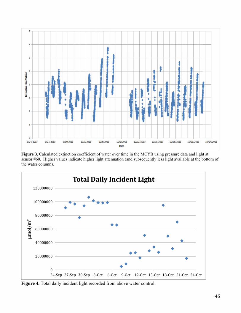
Fst

F

Figure 3. Calsensor #60. Hthe water colu

Figure 4. To

20000

40000

60000

80000

100000

120000

μmol/m

2

culated extincHigher values umn).

otal daily inc

0

0000

0000

0000

0000

0000

0000

24‐Sep 27

ction coefficiindicate high

cident light r

7‐Sep 30‐Sep

Total

ent of water oher light atten

recorded from

3‐Oct 6‐O

DailyIn

over time in thnuation (and s

m above wat

Oct 9‐Oct 1

ncident

the MCYB usubsequently l

ter control.

12‐Oct 15‐Oc

tLight

sing pressure less light avai

ct 18‐Oct 21

data and lighilable at the b

1‐Oct 24‐Oct

45

ht at bottom of

F1

Figure 5. Dai12% incident

ily percent inclight (minimu

cident light atum requireme

t sensor #60, ent for seagra

away from thass production

he shading effn) is the red li

fects of docksine at top

s and most bo

46

oats. The

47

Figure 6. Daily % of incident light recorded under docks. Note: sensor #71 (end of B dock) became obscured by barnacle cover over the course of the experiment; measurements taken after Oct 8 are not shown.

Figure 7. Daily % of incident light recorded from between dock sensors.

0

0.05

0.1

0.15

0.2

0.25

0.3

0.35

0.4

0.45

24‐Sep 27‐Sep 30‐Sep 3‐Oct 6‐Oct 9‐Oct 12‐Oct 15‐Oct 18‐Oct 21‐Oct 24‐Oct

%ofIncidentLight

Date

DailyPercentIncidentLightUnderDocks

SidedockoffC

SidedockoffD

StartofDDock

StartofCDock

StartofBDock

EndofBDock

0

0.05

0.1

0.15

0.2

0.25

0.3

0.35

0.4

0.45

24‐Sep 27‐Sep 30‐Sep 3‐Oct 6‐Oct 9‐Oct 12‐Oct 15‐Oct 18‐Oct 21‐Oct 24‐Oct

μmol/m

2

Date

DailyPercentIncidentLightBetweenDocks

61

62

63

64

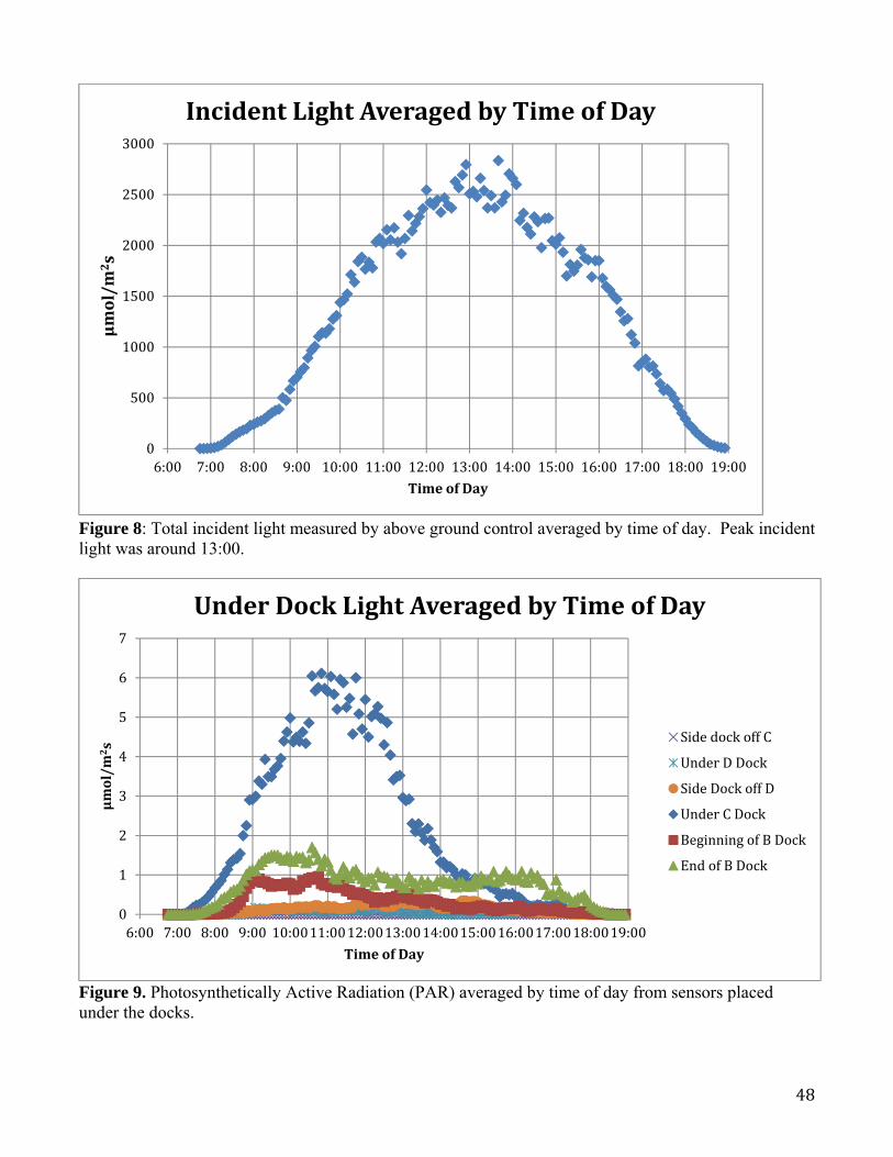
48

Figure 8: Total incident light measured by above ground control averaged by time of day. Peak incident light was around 13:00.

Figure 9. Photosynthetically Active Radiation (PAR) averaged by time of day from sensors placed under the docks.

0

500

1000

1500

2000

2500

3000

6:00 7:00 8:00 9:00 10:00 11:00 12:00 13:00 14:00 15:00 16:00 17:00 18:00 19:00

μmol/m

2s

TimeofDay

IncidentLightAveragedbyTimeofDay

0

1

2

3

4

5

6

7

6:00 7:00 8:00 9:00 10:0011:0012:0013:0014:0015:0016:0017:0018:0019:00

μmol/m

2s

TimeofDay

UnderDockLightAveragedbyTimeofDay

SidedockoffC

UnderDDock

SideDockoffD

UnderCDock

BeginningofBDock

EndofBDock

49

Figure 10. Light extinction curve from LI-Cor PAR sensor, taken around 2 pm. An extinction coefficient of 1.2 L/mol*cm was found.

y=‐1.1896x

‐4

‐3.5

‐3

‐2.5

‐2

‐1.5

‐1

‐0.5

0

0 0.5 1 1.5 2 2.5 3 3.5

ln(I/I0)

Depth(m)

50

Chapter 5: Sediment and Microphytobenthic Community Analysis

1. INTRODUCTION The microphytobenthic layer (MPB layer) consists of photosynthetic microorganisms that colonize the benthic substrata in marine and coastal environments (Macintyre et al., 1996). The MPB layer is an area of intense microbial and biochemical cycling and often is essential in the exchange of nutrients between the water column and the sediments (MacIntyre et al.,1996). The organisms of the MPB layer provide valuable ecosystem services in their respective areas, for example, the benthic algae can contribute up to 50% of primary productivity in estuaries (Underwood & Kromkamp, 1999), can mediate nutrient fluxes between the sediment and water column (Dong et al., 2000), and can provide food for herbivores (Defew et al., 2002). Sediment grain size is the main controlling factor of MPB community assemblage (Perkins et al., 2003, Paterson & Hagerthy, 2001). However, the MPB communities also influence the characteristics of the sediments, creating a relationship between grain size and density of the algal organic matter. Benthic communities help hold sediments together and protect the sediments from resuspension (MacIntyre et. al., 1996; Delgado et al., 1991). The algal communities form a mat on top of the sediments that stabilizes the community. However, if one portion of the mat is disturbed, the integrity of the sheet is damaged and the sediments are exposed to higher velocity flows which increases mean grain size (MacIntyre et. al., 1996). Diatoms dominate fine sediments with smaller grain size ranging from 63 to 125 microns, whereas diatoms dominate sandy sediments with grain sizes of 125 to 500 microns. These sediments may also feature some cyanobacteria and euglenoids (Underwood & Barnett, 2006).

Irradiance is also a factor in benthic community structure because it drives photosynthetic activity. There is a non-linear relationship between photosynthesis and light that depends on light intensity and the irradiance at which the photosynthesis is saturated (Maclntyre et al., 1996). Muddy sediments have a photosynthetically active region (PAR) that reaches approximately 1.3 mm into the top of the sediment, and sandy sediments have slightly deeper light penetration (Kühl & Jørgensen, 1994). The MPB is most efficient at light intensities of 100-800 μmol photons m ⁻ ² second ⁻ ¹. At light levels greater than 1200 μmol photons m ⁻ ² second ⁻ ¹, benthic microalgae migrate deeper into sediments to avoid photoinhibition. We collected and analyzed samples for chlorophyll-a, sediment organic matter (SOM), HPLC, and grain size to uncover any effects of the Morehead City Yacht Basin on the sediments and MPB community within the basin. More specifically, we asked if there was a difference in MPB community assemblage, average grain size, and SOM between the shaded benthos under the floating docks and the un-shaded benthos that is not under the docks. We hypothesized that the docks would not have an effect on chlorophyll-a concentrations, average grain size, or microphytobenthic community structure, and that the docks would have an effect on the sediment organic matter content because of the fouling communities present on the floating docks. We also hypothesized that there would be a difference in MPB community structure and sediment properties between inside the basin and in the channel outside of the basin. The MPB is an extremely important area for photosynthesis, respiration, and nutrient cycling between the sediments and the water column in estuaries, but any impacts on the MPB within the marina would go unseen without scientific analysis of the benthos.

51

2. METHODS

2.1 Sample Collection Inside the Morehead City Yacht Basin (MCYB), twelve cores were taken from a boat and nine were taken from floating docks. Three sample sites were established under each dock, between each dock, and in the channel across from the marina (Fig. 1).

Sediment cores were collected from the MCYB using the Stephenson Apparatus (from the Piehler lab – Fig. 2). This corer uses a clear plastic insert that is exchanged between each sample to prevent cross-contamination. This apparatus has multiple extensions of PVC piping that makes it long enough to reach to the target depth of 2 to 3 meters.

Each large core was subsampled for chlorophyll-a, accessory pigments, sediment organic matter (SOM), and grain size analysis. The cores were pulled onto the boat or dock and the bottom was stoppered with size 13 stoppers to prevent movement and disturbance of the sample. Next, a circular metal disk replaced the stopper on the bottom of the core, and the sample was pushed even with the surface of the corer to remove water and to bring it to a height that was easier to sub-sample. Five cc syringes that had the tops removed to form a cylinder were used to extract the top centimeter of sediment to subsample for HPLC and chlorophyll-a. Each sample was separately placed into labeled 15 ml centrifuge tubes. For SOM, 30 cc syringes were used to extract the subsample. The deepest 4 centimeters and the shallowest centimeter were separated and placed into separate, labeled metal trays. The sediment grain size sample was taken from the remaining core content by pouring approx. 30 grams of sediment into a Whirl-pak. All samples were kept dark and cool in a cooler containing two ice packs until being stored back at the UNC-IMS. Chlorophyll-a and HPLC samples were stored in a freezer at -

20 C. Sediment organic matter was immediately placed into drying ovens for analysis. The sediment

samples were stored in a cold room at 7 C.

2.2 Chlorophyll-a Acidification Processing In the laboratory, chlorophyll-a was quantified using the acidification method and a spectrophotometer (Lorenzen, 1967). The samples were first mixed with a mixture of 45:45:10, acetone, methanol, and diH20, to burst the chloroplast of the cells. Each sample was sonicated for 30

seconds. They were then stored overnight in a freezer set to -20 C to extract the chlorophyll-a. The samples were then poured through a syringe filter with a pore size of 0.7 microns and collected into a cuvette. The cuvette was placed in the spectrophotometer and readings of absorbance at wavelengths of 750 nm and 664 nm were recorded. The cuvette was removed and 100 microliters of 10% hydrochloric acid were added. This further broke down the chlorophyll-a into pheo-pigments. The sample was measured again and readings for absorbance at the wavelengths of 750 nm and 665 nm were recorded.

2.3 Sediment Organic Matter Processing For sediment organic matter, the samples were put into an oven set at 105° C to dry for

approximately twelve hours upon returning to UNC-IMS. They were then weighed to determine the mass of the sediment without the water weight. The samples were then combusted at 525° C for a three-hour period. The combusted material was weighed, and the difference between the combusted and dried sediment revealed the mass of the sediment organic matter. Percent organic matter was determined by dividing the difference of dried mass and combusted mass by the dried mass.

52

2.4 Accessory Pigment Analysis For MPB community analysis using HPLC, sediment sub-cores were placed into 15 mL

centrifuge vials and kept frozen at -20C. The samples were then freeze-dried over a 12-hour period and

returned to the -20C freezer. Each tube was individually covered with aluminum foil to prevent light from degrading sensitive pigments. 3mL of acetone was added to each tube. Samples were immediately sonicated for 30 seconds while held in a beaker with ice water. All samples were again returned to the freezer for 24 hours. Samples were centrifuged for 10 minutes at 5000 rpm. The centrifuge was refrigerated at -20° C. A Millipore syringe driven filter was used to separate the liquid phase (solvent containing pigments) from the solid phase. The resulting liquid was placed into individual 3 mL vials used for HPLC. Samples were stored in -20° C until analysis.

2.5 Sediment Grain Size Analysis Sediment grain size analysis was performed using the Cilas 1180 Particle Size Analyzer. This method implements laser particle size analysis to determine grain size for samples of mostly uniform spherical shape. From each of the 30-gram samples, two rounded scoops, approx. 5 cm3 were taken from the center of the sample with a scoopula. These were taken from the center of the Whirl-pak to obtain accurate average grain size for each sample rather than sampling from the outer sediments that may not be representative of natural patterns. These scoops were diluted with water until they reached a particle concentration at which 8-12% of light is attenuated. This is measured by putting the dilute solution in the Cilas machine and observing the reading from the laser that passes through the sample. Each sample was analyzed to determine average grain size and standard deviation.

3. RESULTS

2.1 Levels of Chlorophyll-a Raw data for all four procedures were collected and analyzed separately as well as in

combination in multivariable analysis. The chlorophyll-a data had an average amount of 89.923 g/L (σ=27.253) (Table 1). There were not significantly lower chlorophyll-a values at the channel site (p=0.822) and no significant detectable differences in sites between docks and under docks (p=0.650) (Table 3).

2.2 Percent Sediment Organic Matter Sediment organic matter percentages were processed for 15 of the 21 sites because there were

some lost in the transfer of trays. The average measurement was 8.131% (σ=3.645) (Table 2). Once again there were significantly lower SOM percentages for the channel (p=0.0081) and not a significant detectable difference in sites between dock and under docks (p=0.371) (Table 3). There were indications of trends between the under dock and between dock locations but there were not enough between dock samples to support the trend.

2.3 Accessory Pigment Analysis HPLC analysis revealed the presence of fucoxanthin and zeaxanthin in all locations of the

MCYB (Table 3). In tests of significance, sample sites I1 and I2 are omitted as the differences in environmental factors (high current velocity and sediment composition) would incur bias in the results. Samples B-D are considered “Under dock” samples, and the letter relates to each floating dock in the

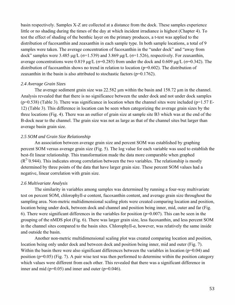
53

basin respectively. Samples X-Z are collected at a distance from the dock. These samples experience little or no shading during the times of the day at which incident irradiance is highest (Chapter 4). To test the effect of shading of the benthic layer on the primary produces, a t-test was applied to the distribution of fucoxanthin and zeaxanthin in each sample type. In both sample locations, a total of 9 samples were taken. The average concentration of fucoxanthin in the “under dock” and “away from dock” samples were 3.485 μg/L (σ=1.539) and 3.869 μg/L (σ=1.526), respectively. For zeaxanthin, average concentrations were 0.819 μg/L (σ=0.285) from under the dock and 0.609 μg/L (σ=0.342). The distribution of fucoxanthin shows no trend in relation to location (p=0.602). The distribution of zeaxanthin in the basin is also attributed to stochastic factors (p=0.1762).

2.4 Average Grain Sizes The average sediment grain size was 22.582 µm within the basin and 158.72 µm in the channel.

Analysis revealed that that there is no significance between the under dock and not under dock samples (p=0.538) (Table 3). There was significance in location when the channel sites were included (p=1.57 E-12) (Table 3). This difference in location can be seen when categorizing the average grain sizes by the three locations (Fig. 4). There was an outlier of grain size at sample site B3 which was at the end of the B-dock near to the channel. The grain size was not as large as that of the channel sites but larger than average basin grain size.

2.5 SOM and Grain Size Relationship An association between average grain size and percent SOM was established by graphing

percent SOM versus average grain size (Fig. 5). The log value for each variable was used to establish the best-fit linear relationship. This transformation made the data more comparable when graphed (R2=0.944). This indicates strong correlation between the two variables. The relationship is mostly determined by three points of the data that have larger grain size. These percent SOM values had a negative, linear correlation with grain size.

2.6 Multivariate Analysis The similarity in variables among samples was determined by running a four-way multivariate

test on percent SOM, chlorophyll-a content, fucoxanthin content, and average grain size throughout the sampling area. Non-metric multidimensional scaling plots were created comparing location and position, location being under dock, between dock and channel and position being inner, mid, outer and far (Fig. 6). There were significant differences in the variables for position (p=0.007). This can be seen in the grouping of the nMDS plot (Fig. 6). There was larger grain size, less fucoxanthin, and less percent SOM in the channel sites compared to the basin sites. Chlorophyll-a, however, was relatively the same inside and outside the basin.

Another non-metric multidimensional scaling plot was created comparing location and position, location being only under dock and between dock and position being inner, mid and outer (Fig. 7). Within the basin there were also significant differences between the variables in location (p=0.04) and position (p=0.05) (Fig. 7). A pair wise test was then performed to determine within the position category which values were different from each other. This revealed that there was a significant difference in inner and mid (p=0.05) and inner and outer (p=0.046).

54

To determine the factors that contributed to the differences in the position and location, a principle component analysis (PCA) was performed on the sampling site factors. The first principle component is the amount of chlorophyll-a that determines the difference in between inner and mid dock positions. The second principle component is percent SOM which determines the difference between dock and between dock locations. The PCA plot shows that the difference in position is determined by chlorophyll-a amount and the difference in location is determined percent SOM (Fig. 8). There was a trend of more percent of SOM under the docks when compared to between the docks locations. The levels of chl-a is lower at the inner position than it is at mid or outer position.

4. DISCUSSION Within the MCYB, there was a significant difference between under the docks and not under the docks, between inner and mid dock positions, and between sample sites within the basin and in the channel. There are many possible dock effects that could suppress the microphytobenthic community. Dock shading could decrease chlorophyll-a under the dock, increased organic matter under the docks is possibly due to the fouling communities present on the docks, and the docks may be slowing currents, which would decrease resuspension of the benthic microalgae. Less chlorophyll-a is present closer to the shoreline surrounding the marina, but fucoxanthin is homogenous throughout the basin, indicating that diatoms are not adversely affected by different factors within the basin controlling chlorophyll-a concentrations. Sediment organic matter was slightly higher underneath the docks than not under the docks, and grain size was approx. homogenous throughout the basin.

Benthic chlorophyll-a measures are widely used as a proxy for primary producer biomass. This method is not an exact measure of primary producer biomass. Chlorophyll-a degrades unless it is kept in complete darkness and sub-freezing temperatures; therefore, the chlorophyll-a amounts that we measured are degraded from levels actually present in nature. Sediment chlorophyll-a measurements in the basin were lower and more variable closer to shore, in what we termed the “Inner” section of the marina. There were also areas of low light (under the docks) within the basin that could theoretically not support microalgae (<1% incident irradiance) (Chapter 4, Fig. 6). Larger current velocities may increase resuspension of the sediments and MPB in the Inner and Outer areas, and lower current velocities in the Mid area could decrease amount of MPB resuspension and allow more light to reach the benthos, resulting in higher chlorophyll-a levels, or more MPB biomass. We accepted our hypothesis that the docks do not have an effect on the amount of benthic chlorophyll-a. Chlorophyll-a was one of the two controlling factors in our multivariate analysis but it determined position within the basin differences rather than difference in dock location (Fig. 8). Also, there was no significant difference between channel sites and sites within the basin. We hypothesized that there may have been a difference in SOM percentage between under the docks and not under the docks because of the fouling communities present on the floating dock structures, and this hypothesis was confirmed. There was an apparent difference in sediment organic matter by location (between under and not under the docks), but no difference in position (inner, mid, outer) within the marina. There was also a statistical difference between sample sites within the basin and in the channel. This difference in location within the basin was only significant in our multivariate analysis, and it was not significant in our one-way ANOVA of SOM values. There were not sediment organic matter samples available for all of the sites, which could have weakened the statistical ability to

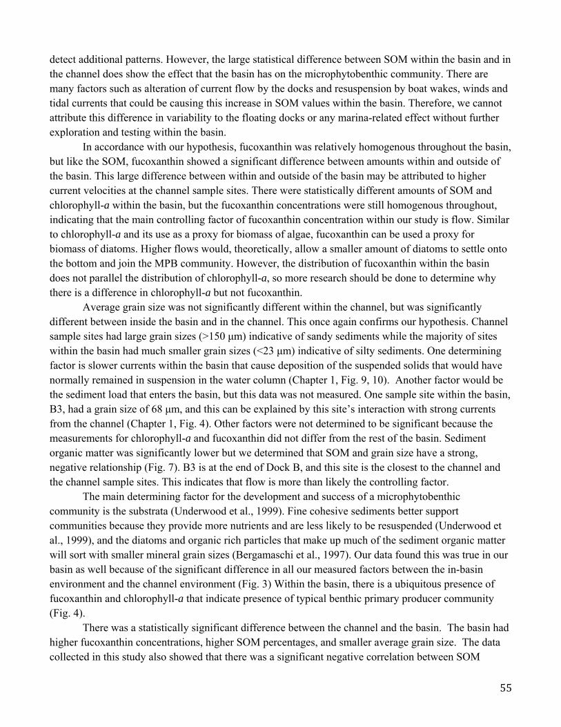
55

detect additional patterns. However, the large statistical difference between SOM within the basin and in the channel does show the effect that the basin has on the microphytobenthic community. There are many factors such as alteration of current flow by the docks and resuspension by boat wakes, winds and tidal currents that could be causing this increase in SOM values within the basin. Therefore, we cannot attribute this difference in variability to the floating docks or any marina-related effect without further exploration and testing within the basin.

In accordance with our hypothesis, fucoxanthin was relatively homogenous throughout the basin, but like the SOM, fucoxanthin showed a significant difference between amounts within and outside of the basin. This large difference between within and outside of the basin may be attributed to higher current velocities at the channel sample sites. There were statistically different amounts of SOM and chlorophyll-a within the basin, but the fucoxanthin concentrations were still homogenous throughout, indicating that the main controlling factor of fucoxanthin concentration within our study is flow. Similar to chlorophyll-a and its use as a proxy for biomass of algae, fucoxanthin can be used a proxy for biomass of diatoms. Higher flows would, theoretically, allow a smaller amount of diatoms to settle onto the bottom and join the MPB community. However, the distribution of fucoxanthin within the basin does not parallel the distribution of chlorophyll-a, so more research should be done to determine why there is a difference in chlorophyll-a but not fucoxanthin.

Average grain size was not significantly different within the channel, but was significantly different between inside the basin and in the channel. This once again confirms our hypothesis. Channel sample sites had large grain sizes (>150 μm) indicative of sandy sediments while the majority of sites within the basin had much smaller grain sizes (<23 μm) indicative of silty sediments. One determining factor is slower currents within the basin that cause deposition of the suspended solids that would have normally remained in suspension in the water column (Chapter 1, Fig. 9, 10). Another factor would be the sediment load that enters the basin, but this data was not measured. One sample site within the basin, B3, had a grain size of 68 μm, and this can be explained by this site’s interaction with strong currents from the channel (Chapter 1, Fig. 4). Other factors were not determined to be significant because the measurements for chlorophyll-a and fucoxanthin did not differ from the rest of the basin. Sediment organic matter was significantly lower but we determined that SOM and grain size have a strong, negative relationship (Fig. 7). B3 is at the end of Dock B, and this site is the closest to the channel and the channel sample sites. This indicates that flow is more than likely the controlling factor. The main determining factor for the development and success of a microphytobenthic community is the substrata (Underwood et al., 1999). Fine cohesive sediments better support communities because they provide more nutrients and are less likely to be resuspended (Underwood et al., 1999), and the diatoms and organic rich particles that make up much of the sediment organic matter will sort with smaller mineral grain sizes (Bergamaschi et al., 1997). Our data found this was true in our basin as well because of the significant difference in all our measured factors between the in-basin environment and the channel environment (Fig. 3) Within the basin, there is a ubiquitous presence of fucoxanthin and chlorophyll-a that indicate presence of typical benthic primary producer community (Fig. 4). There was a statistically significant difference between the channel and the basin. The basin had higher fucoxanthin concentrations, higher SOM percentages, and smaller average grain size. The data collected in this study also showed that there was a significant negative correlation between SOM

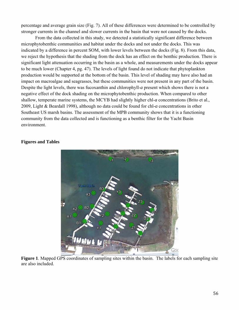
ps

miwstpiDns2Sce

F

Fa

percentage astronger curr

Frommicrophytobndicated by

we reject thesignificant lito be much loproduction wmpact on m

Despite the lnegative effeshallow, tem2009, Light &Southeast UScommunity fenvironment

Figures and

Figure 1. Maare also inclu

nd average grents in the c

m the data colbenthic comm

a differencee hypothesis ght attenuatiower (Chapt

would be supacroalgae anlight levels, tect of the doc

mperate marin& Beardall 1S marsh basifrom the datat.

d Tables

apped GPS cuded.

grain size (Fchannel and llected in thimunities ande in percent Sthat the shadion occurrinter 4, pg. 47)

pported at thend seagrassethere was fuck shading one systems, t1998), althouins. The assea collected a

coordinates

Fig. 7). All ofslower curreis study, we

d habitat undSOM, with lding from thg in the basi). The levelse bottom of ts, but these c

ucoxanthin anon the micropthe MCYB hugh no data essment of thand is functio

of sampling

f these differents in the badetected a s

der the docksower levels

he dock has ain as a wholes of light fouthe basin. Thcommunitiesnd chlorophyphytobenthihad slightly could be fouhe MPB comoning as a be

sites within

rences were asin that werstatistically ss and not undbetween the

an effect on e, and measu

und do not inhis level of ss were not pyll-a presentc productionhigher chl-a

und for chl-ammunity shoenthic filter

n the basin. T

determined re not causedsignificant dider the docke docks (Fig.the benthic purements unndicate that pshading may

present in anyt which shown. When coma concentratia concentratiows that it is for the Yach

The labels fo

to be controd by the docifference bet

ks. This was . 8). From thproduction. der the dockphytoplanktoy have also hy part of thews there is nmpared to othions (Brito eions in othera functionin

ht Basin

or each samp

56

olled by cks. tween

his data, There is

ks appear on had an basin.

not a her

et al., r ng

pling site

Ff TdSBBBCCCDDDXXXYYYZZZ

Figure 2. Scfor collecting

Table 1. Rawdesignated. Sample LB1 UB2 UB3 UC1 UC2 UC3 UD1 UD2 UD3 UX1 BX2 BX3 BY1 BY2 BY3 BZ1 BZ2 BZ3 B

chematic Diag underwater

w data for Ch

Location Under Dock Under Dock Under Dock Under Dock Under Dock Under Dock Under Dock Under Dock Under Dock Between DocBetween DocBetween DocBetween DocBetween DocBetween DocBetween DocBetween DocBetween Doc

agram of the r sediment c

hl-a amount

PosiNeaMidOuteNeaMidOuteNeaMidOute

ck Neack Midck Outeck Neack Midck Outeck Neack Midck Oute

Stephensoncores.

ts per sample

ition Amar 56.d 168er 88.

ar 98.d 102er 94.

ar 55.d 95.er 87.

ar 40.d 84.er 113

ar 98.d 104er 117

ar 48.d 72.er 107

n Apparatus b

e along with

mount of Chl.71 8.39 .71 .27 2.52 .02 .77 .61 .65 .37 .45 3.14 .27 4.11 7.92 .87 .77 7.83

borrowed fro

location and

l-a (ug/L)

om the Piehl

d position pa

ler Lab and

arameters

57

its use

58

I1 Channel Far 67.99 I2 Channel Far 95.08 Average 89.92 Standard Deviation 27.25 Table 2. Raw data for the sediment organic matter percentages per sample along with location and position parameters designated. There was not a complete set of samples sites because some of the samples were lost during processing. Sample Location Position Percent SOM (%) B1 Under Dock Near 10.87 B2 Under Dock Mid 10.22 B3 Under Dock Outer 2.73 C1 Under Dock Near 11.17 C2 Under Dock Mid 7.15 C3 Under Dock Outer 11.04 D1 Under Dock Near 6.45 D2 Under Dock Mid 13.66 D3 Under Dock Outer 11.29 X1 Between Dock Near 8.32 Y2 Between Dock Mid 9.28 Z2 Between Dock Outer 8.33 Z3 Between Dock Near 9.72 I1 Channel Mid 0.71 I2 Channel Outer 1.03 Average 8.13 Standard Deviation 3.64 Table 3. Pigments used for benthic community composition. Sample Location

Sample Weight (g) Analyte Volume(uL)

Total Volume (ml)

Fucoxanthin (µg/ g)

Zeaxanthin (µg/ g)

B1 0.422 200 3 2.566323 0.483428 B2 0.203 200 3 3.496121 1.240853 B3 0.443 200 3 4.943679 0.646774 C1 0.445 200 3 3.301254 0.887073 C2 0.313 200 3 6.637031 1.097324 C3 0.326 200 3 2.661829 0.510288 D1 0.36 200 3 4.439132 1.046181 D2 0.389 200 3 1.916201 1.023594 D3 0.421 200 3 1.404276 0.443374 I1 1.323 200 3 0.393027 0 I2 1.421 200 3 0.444521 0 X1 0.538 200 3 2.702486 0.31291 X2 0.562 200 3 3.076798 0.421832 X3 0.537 200 3 3.93762 0.364097 Y1 0.287 200 3 6.166551 0.707506 Y2 0.292 200 3 6.95097 1.517664 Y3 0.439 200 3 3.764802 0.463086 Z1 0.439 200 3 2.295316 0.495981 Z2 0.32 200 3 2.775215 0.578582

59

Z3 0.341 200 3 3.156851 0.619565 Table 4. One-way, Simple ANOVA of various factors within the MCYB

One-Way, Simple ANOVA

Chl-a, Between all groups Mean SE P-Value Under Dock 94.18245 10.89507228 0.82199 Outside Dock 87.52744 9.374978854Channel 81.53685 13.54521038

Chl-a, Between under dock and not under dock Under Dock 94.18245 10.89507228 0.64959 Outside Dock 87.52744 9.374978854

Chl-a, Between Inner and Mid areas Inner 66.37662 10.3650361 0.0494339 Mid 104.64339 13.6291414

Sediment Organic Matter, Between all groups Under Dock 11.85468 1.779988206 0.0081 Outside Dock 9.52028 0.461262198 Channel 0.7495 0.106562432

Sediment Organic matter, Between under dock and not under dock Under Dock 11.85468 1.779988206 0.37098 Outside Dock 9.52028 0.461262198 Average Grain Size, Between all groups Under Dock 24.39222 5.516938256 1.57E-12 Outside Dock 20.77222 1.633288926Channel 158.1833 4.64 Average Grain Size, Between Under dock and not under dock Under Dock 24.39222 5.516938256 0.538119 Outside Dock 20.77222 1.633288926

Fdl

Fo

Figure 3. HPdocks. The plocation type

Figure 4. Groutlier from

0

20

40

60

80

100

120

140

160

180

GrainSize(µm)

ST

PLC pigmenp-value resules is 0.602. W

raphic distribthe under do

0

1

2

3

4

5

6

Concentration(ug/g)

SedimhreeL

nt between unlting from anWhen the t-te

bution of aveock location

Fucoxan

Avera

entGrLocatio

UnderDock

nder docks an unpaired t-est is applied

erage grain sis the B3 da

nthin

agePigm

rainSionsSa

BetweDoc

and out from-test of fucoxd to zeaxanth

sizes for eacata point clos

Zeaxanth

mentDi

izeforampled

eenck

m an area of exanthin conchin, the p-va

h sampling sse to the cha

hin

istribut

rd

Channel

expected shacentration bealue is 0.176

site of the thannel.

tion

UnderDock

Awayfromd

ading effect etween samp6.

hree location

Avg

dock

60

from the ple

ns. The

FT

FSsc

Figure 5. A This relation

Figure 6. MuSOM, Chl-a show the trenchannel and

Chann

Channel

graph of thenship is contr

ultivariable amounts, fu

nds in locatiother locatio

nel

e log value orolled by thr

analysis nMucoxanthin leon and positons with a p-

f sediment oree of the fou

MDS plot of aevels and gration. There i-value of 0.0

Dock

organic matteurteen sampl

all samples sain size. Thes significanc

007.

TransfoResemb

er over the lles that have

sites, taking ie figure is noce in these fa

orm: Square rootblance: D1 Euclidea

Dock

D

Doc

Dock

Doc

Dock

Do

Doc

Between

Between

Between

Betwe

2D S

log value of e larger grain

into accounton-metric buactors betwe

an distance

Posin

m

o

fa

Dock

kckock

ck

een

tress: 0.01

average grain size.

t factors of p

ut the groupineen the locat

itionnner

mid

uter

ar

61

in size.

percent ngs ion of

62

Figure 7. Multivariable analysis nMDS plot of samples sites without the channel sites, taking into account factors of percent SOM, Chl-a amounts, fucoxanthin levels and grain size. The figure is non-metric but the groupings show the trends in location and position. There is significance in these factors between the locations with a p-value of 0.04 and position with a p-value of 0.05.

Figure 8. Multivariable analysis PCA plot for nMDS plot in Figure 7. This shows the 15 sample site with four components of Chl-a amounts, fucoxanthin levels, grain size and percent SOM. The first principle component is amount Chl-a that determines the difference in between dock and under dock

Transform: Square rootResemblance: D1 Euclidean distance

Positioninnermidouter

Dock

Dock

Dock

Dock

Dock

DockDock

DockDock

Between

Between

Between

Between

Between

Between

Between

BetweenBetween

2D Stress: 0.1

-4 -2 0 2 4PC1

-2

0

2

4

PC

2

Positioninnermidouter

Dock

Dock

Dock

Dock

Dock

Dock

Dock

Dock

Dock

Between

BetweenBetween

Between

Between

BetweenBetween

Between

Between

Chl-a (ug/L)

SOM (%)

Fuco (ug/g)

Grain Size (um)

63

locations. The second principle component is percent SOM which determines the difference between inner and mid position (p=0.05) and between inner and outer positions (p=0.046).

64

Chapter 6: Fouling Organisms and Fish Communities

1. INTRODUCTION Epibiota are the plants and animals that attach to hard surfaces (Clynick et al., 2007). Epibiota play a vital role in providing a biotic structure on the surface of an artificial substrate, which can enable further colonization of species. Floating dock structures provide habitats for a large number of subtidal plants and animals that would normally be attached to a rocky reef (Connell & Glasby, 1999). A study in Sydney Harbor, Australia revealed that urban habitats create novel habitats for epibiotic assemblages regardless of the composition of the substratum (Connell, 2001). Connell & Glasby (1999) also indicate that artificial structures may increase the abundance and diversity of subtidal epibiota, but are not an exact substitute for epibiotic assemblages that occur on nearby natural substrates. Therefore, there is growing concern that urban structures do not adequately replace natural reefs and could support epibiota that would not otherwise naturally settle. Artificial structures that provide novel habitat for flora and fauna have the potential to attract herbivorous and carnivorous fish species because epifauna living in the biota attached to structures may be a source of food (Lopez-Jamar et al, 1984). Investigations of epibiota population dynamics indicate that habitats created due to beach development can contribute to increasing fish biomass (Bohnsack, 1989; Fabi et al., 2004) and abundances (Rooker et al., 1997). Epifauna and epiflora may also provide protection for small fish species such as adult blennies and juveniles as they seek refuge from predators. However, not all studies support these claims. Coleman & Connell (2001) experimentally removed epibiota from pier pilings and found that the variation in the amount of epibiota had only minor effects on the abundances of fish around pilings. Therefore, it is necessary to employ caution when making generalizations regarding the value provided to epibiota by artificial habitat structures because such relationships can be location-specific. The first part of the present study investigated factors that govern epibenthic assemblage structure in the Morehead City Yacht Basin. We hypothesized that there would be a significant difference in the floating dock communities based upon the directions in which the floats face (aspect) and distance from land. This hypothesis was tested by taking and analyzing scrape samples from the floating docks at several locations throughout the marina. The second part of this study investigated how the Morehead City Yacht Basin acts as a habitat for fish species in an urban coastal ecosystem. The goal was to identify spatial patterns in the distribution and abundance of fish within the marina. Specifically, we tested the hypothesis that the behavior and composition of fish assemblages would differ within the marina. We predicted that fish species would utilize all of the floating docks for refuge and food, but that currents and distance from land would explain the variation in species abundance throughout the marina. To determine the generality of these patterns, this hypothesis was tested at several locations and during high, ebb, and low tides. In order to further describe overall anthropogenic effects of the marina on the ecosystem, we juxtaposed our epibiota and fish abundance data with the light, current, and dock orientation data gathered by other groups.

65

2. METHODS

2.1 Scrape Analysis We completed an assessment of the epibiota within the Morehead City Yacht Basin to explore ecological gradients and interpret the effects of dock aspect, dock orientation, dock location, tides, and current flow on the characteristics of the dock communities. This assessment was completed by performing a scrape analysis. We determined the scraping sample locations by using a stratified random sample of Dock B, Dock C, and D-dock (Figure 1). We divided each dock into three sampling strata based on distance from land (near, mid, far) and within each strata we randomly chose two sampling locations based on the boat slip numbers. To make sure we included the ends of the dock, we also took four haphazard samples at the end of B, C, and D docks. Our design yielded a total of 22 sampling locations (Figure 1). However, a single sample was lost due to processing error (n=21). At each location, we used a 25 cm by 25 cm PVC (20 mm diameter) quadrat to standardize and designate the scraping sample space. The quadrat was held against the vertical float surface in a haphazardly-chosen location within the aforementioned slip numbers. We used a 5 mm mesh size net supported by a 1 m2 square frame of PVC (20 mm diameter) pipes to collect falling organic material as they were scraped off of the float surface using a 15 mm x 25 mm square metal spatula. Each sample was bagged, labeled and placed in a cooler with ice. Samples were then transported to the lab where they were stored in a walk-in cooler (7ºC) to preserve the samples. Within 24-48 hours of collection each sample was deposited into a white tray and rinsed with saltwater collected from Bogue Sound. Species were sorted and individuals were counted while colonial species were quantified by weight using a top loading balance or by measuring the surface area. Using marina blueprints, an estimate of the total float surface area available to the epibenthic communities was calculated in order to estimate the total biomass of colonial species in the marina.

2.2 Fish Abundance and Behavior To qualitatively assess the fish species abundance and behavior at the marina, our group made observations along the docks during high, mid, and low tides and identified fish species based on visual characteristics. Two observers spent five minutes at each of the designated near, mid, far, and end portions of the dock recording fish species. To record fish abundances, a scale adopted from the Reef Environmental Education Foundation (2013) roving diver survey technique was used: S (single; 1), F (few; 2-10), M (many; 11-99) and A (abundant; 100+). One observer monitored one side east of the dock while the other monitored the western side. Observers then switched sides after each five-minute trial. This method was used for the three docks under study and for the three chosen tide phases. In addition, the observers qualitatively recorded swimming patterns and direction, habitat use, and other general observations. Observations were only made for one day (n=1) and visibility was often limited.

3. RESULTS

3.1 Scrape Analysis To supplement the dispersion and variability statistics for the scrape data, dominant taxa were

subjected to an analysis of variance of their abundance or mass relative to their dock (B, C, or D), their relative position (inner, mid, outer, end), and their float aspect (north, east, or west). ANOVA tables

66

were produced using R-statistical software. For all of the ANOVA tests, significant results were found to exist for Codium fragile between the parameters of mass and aspect (p=0.0136), as well as the parameters of mass and position (p=0.0393) (Table 5). The difference in the means between shrimp species with respect to aspect was also significant (p<0.05). There were only two samples that contained Codium, both of which were taken at the north-facing end position of Dock C. Both of these samples also contained shrimp. Although these results indicate a tight coupling between shrimp and Codium, the paucity of data limits the extent to which significant conclusions between the two species may be drawn.

Species richness, the number of different species per scrape sample, was averaged for each dock, aspect, and position relative to land (Figure 2). Although there was slightly greater species richness on Dock B, on eastern facing slips, and at outer points compared to other measured points around the marina, these differences were not statistically significant (p>0.05).

In order to gain a better understanding of the epibiota community species distribution throughout the marina, we examined the colonial species mass data. Of the approximately 1.19 kg of total colonial species collected from the scrape samples, Codium fragile constituted the largest percentage (41.2%) of colonial species mass, closely followed by Bugula spp. (37.6%) (Figure 3). Further analysis of wet mass for each parameter was conducted to examine the spread of the colonial species relative to dock, aspect, and position (Figure 4). Compared to the other docks, Dock C had the greatest colonial species mass (approximately 808 g). Codium fragile constituted approximately 65% and Bugula spp. approximately 25% of the total mass for Dock C. The samples collected from the north-facing slips had an overall greater mass than those facing east and west, in large part due to the presence of Codium (83% of total mass). West-facing slips had colonial species mass made up of nearly 38% Porifera spp. while east-facing slips only had approximately 5% sponge. The ends of the three docks had the highest overall wet mass (589 g) compared to the other dock positions. Because Codium spp. colonies are on average denser than the other colonial species present at the marina, this may have contributed to the greater combined mass for the north-facing end positions on Dock C. If the two Codium species found in the scrape samples were not included in the data, the far slips, west aspect, and Dock C would have the greatest mass. Therefore, it is important to note that although Codium fragile contributes such a high percentage to total colonial species mass, it occurs so infrequently that its relative importance to the overall epibiota community may be limited. Lastly, using dock and float surface area measurements, we estimated that approximately 2555 kg of colonial epibiota are supported by the yacht basin’s floating docks (Table 1).

Relative abundance and distribution for each species was calculated for each dock, aspect and position. Relative species abundance is denoted by percent by mass or count depending upon the feasibility of quantifying each species (Table 2). Species distribution, denoted by percent presence for each 625 cm2 quadrat, was also calculated for each species (Table 2). Neither species abundance nor distribution is statistically significant between any of the factors. Bugula spp., Tunicata spp., C. virginica, and Ulva spp. were evenly distributed between the inner, middle, outer, and end locations of the docks, but approximately 50% of each species’ mass was found on the eastern side of the docks. Bugula spp. had the lowest abundance (13%) at Dock D, and the lowest abundance of Ulva spp. was found at the inner dock positions (8%). Balanus spp. were fairly evenly distributed among the dock, dock position, and aspect parameters. B. exustus was present in several locations and showed greater abundances on eastern slips (56%), on Dock B (64%), and in the middle positions (49%), compared to other aspect, dock, and position options. B. anisotoxa presented abundances at inner locations (90%), on

67

west-facing slips (90%), and on Dock C (51%) that were much greater than other parameter options. B. anisotoxa was not found at the end and outer dock positions. 100% of Codium spp. abundances and 96% of shrimp abundances were concentrated at the north end of Dock C. In addition, 49% of the crabs were found on the west side of Dock C, while crabs were least abundant (only 9%) at the north-facing ends of each dock.

Analyses revealed no clear effect of dock orientation and position on the epibiota community composition. Distance-based tests for homogeneity of multivariate dispersions using PRIMER 6 software and the PERMDISP built-in function were performed on square-root transformed data of combined epibiota taxa. These tests yielded statistical significance (p=0.021) between the variability among community composition with regard to sample position (Table 3). Subsequent pairwise comparisons revealed significant differences in variability between the following positions: end and inner (p=0.036), end and outer (p=0.014), mid and outer (p=0.045), inner and outer (p=0.017) (Table 4). The inner section is moderately variable as compared to the end and mid positions. The outer position was the least variable (but contained only three sample points). However, when the dock parameter was inputted as the contributing factor in this same test, no significant interaction between specific dock and community structure was shown (p=0.851) (Table 3). Moreover, there was evidence that the abundance of Brachidontes exustus and Balanus spp. were the drivers of this variability; however, they did so independently (Figure 5).

3.2 Fish Abundance and Behavior The most common pelagic fish species observed at the Morehead City Yacht basin were Menidia menidia (Atlantic silverside), Anchoa mitchilli (bay anchovy), Lagodon rhomboides (pinfish), and Archosargus probatocephalus (sheepshead). At slack-high tide, there were approximately the same number of silversides and/or bay anchovies (the two could not be distinguished from the docks) at all three docks and they tended to reside approximately 1-1.5 meters from the floating dock structure at a depth of less than 0.25 m. D-dock evidenced the most balanced silverside and/or bay anchovy abundances in relation to aspect and distance from land (Figure 6). Stationary schools favored the east side of Dock C and Dock D. In comparison, more active and larger schools of silversides and/or bay anchovies were located on the west side of Dock B. The larger and more active schools were located farther away from the dock (3-4 m) and at a greater depth (>0.5 m), and their behavior indicated swimming behavior rather than foraging behavior. Pinfish were observed less frequently than silversides and/or bay anchovies and were more evenly spaced within the marina at high tide (Figure 6). Two sheepshead fish were observed at a vacant slip under the east side Dock C. During mid-ebb tide, silversides and/or bay anchovies were still the most prevalent fish species sighted at the marina (Figure 6). Large schools of bay anchovies and/or silversides were observed on the west side of Dock B and were traveling north to south, opposite the general schooling direction observed during high tide. There were fewer silversides and/or bay anchovies near the end of the docks and closer inland during mid-ebb tide. Pinfish abundances were much lower during mid-ebb tide throughout the marina with no detectable distribution pattern while showing a similar foraging behavior as during high tide (Figure 6). A single sheepshead was observed on the west side of Dock C closer to shore. At slack-low tide, even fewer silversides and/or bay anchovies were observed. Silversides and/or bay anchovies were concentrated inland and exhibited similar behavior as those during high and ebb tides (Figure 6). A single, less active school of silversides and/or bay anchovies was observed off of the

68

west side of Dock B. In no discernible pattern, single pinfish were observed throughout the marina (Figure 6).

Anecdotal evidence of other marine life in and around the marina was provided by marina slip owners. These individuals told of a porpoise sighting outside of the marina in June 2013, sea otter sightings during the summer months of 2013, and the aggregation of feeding fish at night, a pattern that was suggested to be effected by the marina lights during the night. In addition, a plethora of stone crabs were found on and inside of cinder blocks deployed for the light attenuation data, suggesting that the epibiota can also support large benthic crustaceans within the basin.

4. DISCUSSION

The goal of this study was to examine the characteristics and spatial trends of epibiota and fish assemblages within the Morehead City Yacht basin in order to interpret the role of the floating docks as a habitat for marine organisms. It is apparent that the docks support a diverse and abundant community of marine species, as almost no bare space was sighted on the surface of the submerged floats. Interestingly, we found few significant trends in epibiota community composition, species richness, and species abundance within the marina relative to dock aspect, position relative to land, and the docks under study.

The distance-based tests for homogeneity of multivariate dispersions revealed the significant impact of position on the variability of community structure. This test showed that the variability of the community structure was greatest at the end and mid dock positions and that the outer position showed the least variability. This may have been a result affected by a lesser number of collected samples at the outer position, in comparison with other positions. There was no overlying pattern relating community variability to the sample site’s proximity to the shore or channel. However, there were some positions (end, mid) that showed significantly greater variability compared to other positions. The end of B dock experiences stronger and more variable flows compared to other locations (Chapter 1, pg. 11). Stronger flows may create a physically stressful environment causing haphazard removal of species living on the floating dock. As supported by Sutherland and Karlson (1977), the recruitment of new settlers to unoccupied space varies based upon the time of year, placing community structure in a state of constant flux with the unpredictable threat of removal.

The majority of the ANOVA tests between individual epibiota species and dock, aspect, and position did not yield significant results. These findings indicate that the parameters of dock choice, aspect, and position relative to land exert a minimal impact upon species in the marina’s epibiotic communities. Because the lack of significance for such factors does not reveal any further insight into the effectiveness of the floating docks as a substrate for epibiota, trends throughout the marina that were observed during the sampling period can be used to describe the general characteristics of the communities. For example, it is evident that the floating docks provide a surrogate substrate; from our general observations during our scrape analysis we rarely saw more than 10% bare space on the floats. Also, the barnacles and oysters settled directly on the float substrate, which may drive succession and recruitment by providing greater surface area for the settlement of other epibiotic species capable of settling on secondary substrate. Another noteworthy find was that 96% of shrimp individuals found during our scrape analysis were located directly on the Codium fragile. This suggests that the shrimp

69

may utilize this macroalgae for refuge from predators, a food source, or protection from the high flow environment.

The concentration of Ulva spp. greatly depends on the amount of sunlight available (Altamirano et al., 2005). Although higher concentrations of Ulva spp. were observed on the east side of the docks and the lowest concentration of Ulva spp. was observed in inner parts of the dock. Balanus spp. have increased tolerance to adverse environmental conditions which may explain the species’ more evenly spaced distribution around the marina (Desai, 2009). It is unclear why B. anisotoxa was most abundant on the inner positions (90%) and the west sides (90%) of the docks.

Crabs that favored the west side of Dock C, where fish were least abundant during high tide, may have found protection and decreased predation from sheepshead that feed on invertebrates (Hernandez & Motta, 1997). Future studies could measure crab abundances during different tidal stages to provide insight into whether the locations of crabs were related to current direction.

For all observation periods, the silversides and/or bay anchovies favored the inland east side of all three docks. Although we did not measure flow on the fish survey day, our direct observations from the docks suggested flow was slower on the east side of the docks both at high and low tides perhaps providing regions for fish to escape the highest flow velocities.

The majority of the observed silversides and/or bay anchovies were located inland during ebb tide. The inland portion of the marina receives lower flow rates, therefore fish may occupy this area to reduce energy exertion (Chapter 1, Fig. 9). Another recurring observation was that the silversides and/or bay anchovies tended to school behind the pilings on the east sides of docks. During ebb tide, marina current flow followed a west to east pattern, therefore fish would find slower current and protection behind the east side of the pilings (Chapter 1, Fig. 9). Pilings attract plankton from all depths and provide an aggregated food source as well as protection from predators (Clynick, 2008; Hamner et al., 1988). No obvious distribution was seen for the pinfish or sheepshead; however, they were always observed to be feeding directly on the floating dock epibiota. Also, very few fish were detected in boat slips with chemical slicks and visible trash pollution contained between the dock float and the stern of the boat. It is possible that this pollution could have interfered directly with fish behavior by acting as a deterrent. For example, pinfish have been known to effectively learn to avoid consumption of material through trial and error (Lopanik et al., 2004). The pinfish and other fish species may have learned to avoid the polluted areas in a similar manner.

Dock D evidenced the most balanced silverside and/or bay anchovy abundances in relation to aspect and distance from land. Clynick (2008) attributed the increased abundance and diversity of fish at Davis Marina, Sydney, Australia to the relative proximity of the marina to a natural rock reef. Likewise, we attribute the higher abundance of fishes on Dock D to the dock’s proximity to a salt marsh bordering the east side of the marina. Salt marshes are sites of deposition of sediments and organic matter that could provide a food source to fishes utilizing Dock D (Koch et al., 2009).

Our findings support the claim that artificial structures have a strong effect on fish spatial distributions (Clynick, 2008). Fish are likely to be attracted to the marina since it provides a form of shelter, protection from predators and food source (Edgar, 1999; Mobley & Fleeger, 1999; Hixon & Beets, 1993). Other studies have suggested that fish biomass increases in the presence of artificial structures such as marinas (Bohnsack, 1989; Fabi et al., 2004). However, because only one day of

om

svwt

dahsdsshmp

F

F2d

observationsmore signific

The yserve as a suvalue to the ewere likely tthat support

Humdecline and eand terrestriahabitat for a sheepshead. docks presenstudied suppstructures. Mhabitat directmarina may hprovides nov

Figures and

Figure 1. An28557. Circldock epibiota

were made cant analysisyacht basin prrogate subsecosystem bo consume eepibiota in than alterationextinction, anal communitvariety of mBoth the scr

nt a valuableort an estima

Moreover, mtly on dock fhave initially

vel habitat an

d Tables

nnotated diages indicate ra on Docks B

(n=1) and vs of fish behaprovides a unstrate for the y filtering th

epibiota attache marina, b

n of the naturnd understanties is critica

marine specierape analysis habitat for oated 2500 kg

many other nofloats. We coy been destrnd indirect b

gram of the randomly genB, C, and D.

visibility wasavior and renique habitaepibiota and

he water thatched to pilinbut do not neral environmnding the rol

al. The Morees, from filtes and fish aborganisms. Tg of colonialon-colonial sonclude that

ructive to thebenefits for a

Morehead Cnerated slip .

s often limitesponse to do

at for variousd many of tht is rich withngs and floatecessarily exment is increale of artificiahead City Y

er-feeding enbundance andThe docks sel species, andspecies sucht although the natural suba host of epib

City Yacht Bnumbers cho

ed, more triaock presences marine orghe epibiotic oh TSS and nuts, which wexclusively deasingly citedal surfaces a

Yacht Basin cncrusting spod behavior aerve as a subd fish were c

h as barnaclehe constructibstrata, the prbiotic and pe

Basin. 2208 Aosen for scra

als are necese. ganisms. Theorganisms liutrients (Chaere some of tepend upon td as a driver as alternate hclearly provionges to the analysis indicbstrate for epconcentrateds and crabs a

ion and redevresence of thelagic specie

Arendell St, ape sampling

sary to prov

e floating doike bivalves apter 2, pg. 2the only struthe epibiota of populatio

habitats for mides a structuomnivorous

cate that floapibiota, as thd near the also find suivelopment ohe floating des.

Morehead Cg of the floa

70

vide a

cks provide

23). Fish uctures

for food. on marine ural s ating

he docks

itable of the docks

City, NC ating

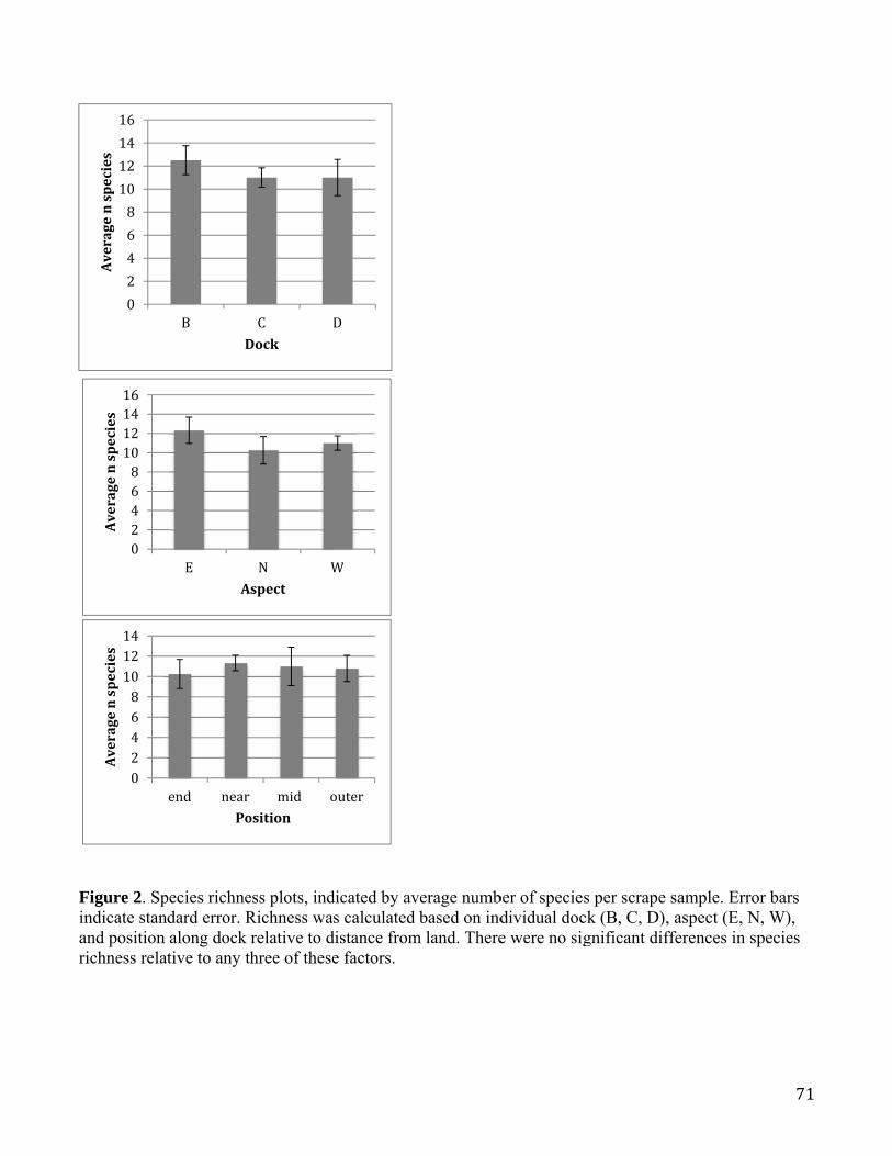
Fiar

Figure 2. Spndicate stan

and position richness rela

0

2

4

6

8

10

12

14

16Averagenspecies

0246810121416

Averagenspecies

02468101214

Averagenspecies

pecies richnedard error. Ralong dock tive to any th

B

D

E

A

end near

Po

ess plots, indRichness wasrelative to dhree of these

C D

Dock

N W

spect

mid o

osition

dicated by avs calculated

distance frome factors.

D

W

outer

verage numbbased on ind

m land. There

ber of speciesdividual doce were no sig

s per scrape ck (B, C, D),gnificant dif

sample. Err, aspect (E, Nfferences in s

71

ror bars N, W), species

72

Figure 3. Pie chart representing percentages of Bugula spp., Codium spp., Ulva spp., Porifera spp., and other colonial species relative to the entire wet mass of colonial species sampled from the floating dock epibiota communities.

37.60%

41.24%

9.32%

10.96%

0.87%

TotalColonialSpeciesWetMassBugula Codium Ulva Porifera Other

73

Figure 4. Wet masses of colonial species relative to individual dock, aspect, and position on the dock relative to distance from land.

0100200300400500600700800900

B C D

Mass(g)

Dock

Other

Porifera

Ulva

Codium

Bugula

0

100

200

300

400

500

600

700

E N W

Mass(g)

Aspect

Other

Porifera

Ulva

Codium

Bugula

0

100

200

300

400

500

600

700

end far mid inner

Mass(g)

Position

Other

Porifera

Ulva

Codium

Bugula

Fv

Figure 5. Privariability dr

incipal Comrivers were l

mponents Analikely musse

alysis plot gls and Balan

enerated fronus (barnacle

m PRIMERe) spp.

R 6 software

showing tha

74

at

FmLa

Figure 6. Dimid, and lowLagodon rhoand Abundan

igital image w-slack tidesomboides (Pint (100+) sca

of the Moreh. Menidia minfish) abundale.

head City Yenidia (Atladances are d

acht Basin fantic Silversidenoted using

for fish obseride), Anchoag the Single

rvations mada mitchilli (B

(1), Few (2-

de at high-slBay Anchovy-10), Many (

75

lack, y), and (11-99),

76

Table 1. Data summary of dock surface area, estimated float surface area, and total colonial species wet mass collected from the scrape samples. From this data, an estimate of the total wet mass of colonial species supported by the floating docks as the marina was calculated.

Dock Dock surface area (cm2)

Float surface area (cm2)

Total wet mass (g)

B 8.85E+06 1.18E+07 289.30

C 6.80E+06 9.04E+06 808.60

D 3.11E+06 4.14E+06 93.11

Other 2.42E+06 3.21E+06 N/A

Total 2.12E+07 2.82E+07 1191.01

Total n 21 Surface area (cm2) /n 625 Mean wet mass (g)/ cm2 9.07E‐02 Estimate total wet mass (kg) 2.56E+03

Table 2. Relative species abundance (denoted using percentages of total mass or count) and species distribution (denoted percent by presence) for each dock, aspect and position. Relative abundance of B. anisotoxa found on Dock B excludes a negligible mass in percent by mass calculation that is considered in distribution presence/absence percentages.

Bugula spp.  Tunicata spp.  C. virginica  Balanus spp.  B. exustus  Ulva spp.  B. anisotoxa  Codium spp.  Shrimp  Crab 

  % by mass 

% Pres. 

% by count  % Pres. 

% by count  % Pres. 

% by count  % Pres. 

% by count  % Pres. 

% by mass  % Pres. 

% by count  % Pres. 

% by mass  % Pres. 

% by count 

% Pres. 

% by count  % Pres. 

B  41%  29%  33%  30%  23%  32%  32%  29%  64%  32%  45%  33%  39%  33%  0%  0%  0%  0%  21%  21% 

C  45%  38%  42%  40%  38%  32%  34%  38%  26%  42%  37%  40%  51%  33%  100%  100%  96%  67%  49%  43% 

D  13%  38%  25%  30%  39%  37%  34%  33%  10%  26%  17%  27%  10%  33%  0%  0%  4%  33%  30%  36% 

E  49%  43%  50%  45%  48%  47%  38%  43%  56%  42%  50%  40%  10%  33%  0%  0%  0%  0%  42%  50% 

W  35%  38%  37%  40%  30%  37%  44%  38%  25%  37%  25%  40%  90%  67%  0%  0%  4%  33%  49%  36% 

N  16%  19%  14%  15%  22%  16%  18%  19%  20%  21%  24%  20%  0%  0%  100%  100%  96%  67%  9%  14% 

Inner  16%  29%  20%  30%  26%  32%  18%  19%  5%  26%  8%  20%  90%  67%  0%  0%  0%  0%  35%  29% 

Mid  31%  29%  33%  30%  28%  32%  26%  29%  49%  32%  36%  33%  10%  33%  0%  0%  0%  0%  19%  21% 

Outer  37%  24%  34%  25%  24%  21%  24%  29%  26%  21%  32%  27%  0%  0%  0%  0%  4%  33%  37%  36% 

End  16%  19%  14%  15%  22%  16%  33%  24%  20%  21%  24%  20%  0%  0%  100%  100%  96%  67%  9%  14% 

77

Table 3. Variability of community structure with regard to scrape sample position by deviance from centroid. Group Factor F-value P-value Position 5.6483 0.021

Dock 0.2099 0.851

Table 4. Pairwise comparisons between dock position for square-root transformed epibiota data.

PAIRWISE COMPARISONS

Groups P-value (end,mid) 0.89

(end,inner) 0.036

(end,outer) 0.014

(mid,inner) 0.127

(mid,outer) 0.045 (inner,outer) 0.017

Table 5. ANOVA table for Codium fragile mass relative to aspect and position. Both factors yield statistically significant p-values.

Codium fragile Df F value Pr(>F)

Aspect 2 5.514 0.0136

Residuals 18

Codium fragile Df F value Pr(>F)

Position 3 3.472 0.0393

Residuals 17

Chapter 7: Synthesis

Summary of Main Findings

After analysis of the individual components of the marina basin, it is important to consider the environment as a whole. The two questions addressed in the investigative research were whether the docks had any impact and whether the marina as a whole had

78

an impact on the quality of the basin. We looked at both the physical and biological interactions within the marina.

Data revealed there was extreme light attenuation within the basin that is highly variable and very loosely related to possible dock effect shading. This attenuation is better explained by the high levels of total suspended solids (TSS) that were found within the basin. The TSS measured 0.5 meters from the bottom within the basin were much higher than the limit set by NCDENR as well as higher than values from samples in New River collected by Paerl Lab. The TSS found at the surface were not as concentrated within the basin compared to outside the basin. High levels of TSS in the basin may be the result of frequent re-suspension of sediment from current movements. The sediment grain size analysis revealed very fine sediments that are the size of silts and clays within the boundaries of the basin (Chapter 4, Fig. 4). These smaller particles are more likely to be re-suspended through the proposed mechanism of currents thus increasing TSS levels near the bottom. These physical factors combine to create the low light and high suspended solid environment of the basin.

Water quality data analysis showed that TSS values for surface samples were found to be consistently in the 20-40 mg/L range while bottom samples were regularly in the 60-80 mg/L range (Chapter 2, Fig. 3 and Chapter 3, Fig. 6). TSS values appear to be lower during flood tide and higher during ebb tide for both the surface and bottom values which may be indicative of suspended sediments being brought in from Calico Creek during ebb tide. Higher levels of chlorophyll-a and nutrients were also found during ebb tide. The channel currents during flood tide were shown by the physical group to be much faster than waters that leave the basin during ebb tide. These data suggest that slower moving water at ebb tide may be drawing on incoming waters from Calico Creek leading to relatively large concentrations of the above measured parameters.

The levels of light attenuation at the bottom of the basin do not indicate a high enough light level to support phytoplankton growth, but the sampling has shown that there is a benthic mat present. This leads to the conclusion that the primary producers present in the microphytobenthic community are sufficiently resuspended by currents and boat traffic to allow them access to the light that penetrates the water column. Despite the high TSS levels and high light attenuation, the basin supports a microbenthic community that is equal to standards found in literature (Brito et Al. 2009, Light and Beardall 1998). These levels of light and fine sediments do not support macrophyte growth (Hizon-Fradejas et al. 2010). Light and sediment restrictions structure the microphtytobenthic community.

As stated before, there was no negative impact detected on the epibiota and fish from the presence of floating docks. The positive effects of increased surface area, settling, and possible shedding of organisms off the dock to the benthos are a phenomenon worth noting. The large floats underneath the dock provided large areas for epibiota settlement and contained a large amount of wet mass, approximately 2500 kg.

79

This mass was described as being easily removed and susceptible to displacement by drag from strong currents or wake. The transport of organic mass from the floats to the benthos provides a mechanism for maintaining a high abundance of invertebrate species in the yacht basin. The organic matter from epibiota provided detritus and nutrients for the benthic community. Large stone crabs were observed to be hiding in the cinder blocks used to fix light sensors to the bottom of the basin. Also, a few unidentified species of shrimp, polychaete worm, and small crabs had settled on all available space of other equipment deployed in this experiment. The presence of these species and their rapid settlement in depths of light inhibition suggest that source water and nutrient rich, detritus rain from docks are providing valuable nutrient flux to these benthic invertebrates. Therefore, benthic invertebrate limitations may be related more to sediment type and lack of available substrate, not available food.

As a whole, the marina basin ecosystem is not detectably impacted by the floating docks or the marina presence. Some positive impacts have come from increased hard substrate available for the fouling communities that would not have otherwise existed. Microbial activity was well below the level of health concern for NC based on EPA recreational water quality criteria. The nutrient levels and chlorophyll-a levels in the basin are normal and similar to healthy levels found in Pamlico Sound. These levels are also well below the state standard for water quality as established by the North Carolina Division of Water Quality. There was little nitrate detected within the basin and channel but comparably greater amounts of ammonia. These levels of ammonia compared to organic nitrogen is indicative of healthy biological activity and productivity. Benthic analysis revealed the presence of a microphytobenthic community equal to that found in other current literature (Brito et Al. 2009, Light and Beardall 1998). Fucoxanthin was present throughout the basin and channel illustrating diatom communities. Diatoms are a preferred food source for higher order consumers and are indicative of healthier, better mixed water columns. In conclusion, the investigative research of the physical and biological components of the marina basin has revealed that the marina has no detectable negative impact on the environment when compared to the other current literature and relevant data.

Acknowledgements Special thanks should be given to all research partners in this study, without whom this project could not have achieved any sort of success. Thanks also goes to research mentors Dr. Fegley and Dr. Rosman for their patience in long days of assisting with research questions and many hours spent around the marina with the students. Thanks also goes to IMS faculty and staff who helped provide resources and guidance to conduct analyses and push groups to discover more. Thanks also goes to Captain Joe Purifoy for driving the boat all around the marina over numerous days. Finally, we should acknowledge the help and support provided by the staff and administration of the Morehead City Yacht Basin who permitted all sorts of odd activities in the marina throughout the fall.

80

References Altamirano, M., Flores-Moya, A., & Figueroa, F. L. (2000). Long-term effects of natural sunlight under various ultraviolet radiation conditions on growth and photosynthesis of intertidal Ulva rigida (Chlorophyceae) cultivated in situ. Botanica Marina, 43(2), 119-126. Barcina, I., Gonzalez, J. M., Iriberri, J., & Egea, L. (1990). Survival strategy of Escherichia coli and Enterococcus faecalis in illuminated fresh and marine systems. Journal of Applied Microbiology, 68(2), 189-198. Bare, R., Guidroz, K., McCann, K., & Bohanon, C. (2013). Effects of wet and dry

weather events on bacteria (Enterococci) levels and detection of hotspots in a brackish water marina in Texas.

Bergamaschi, B. A., Tsamakis, E., Keil, R. G., Eglinton, T. I., Montluçon, D. B., & Hedges, J. I. (1997). The effect of grain size and surface area on organic matter, lignin and carbohydrate concentration, and molecular compositions in Peru Margin sediments. Geochimica et Cosmochimica Acta, 61(6), 1247-1260.

Berman, J. (2009, October 29). WHO: Waterborne Disease is World's Leading Killer. VOA - Voice of America English News. Retrieved September 21, 2013, from http://www.voanews.com/content/a-13-2005-03-17-voa34-67381152/274768.html

Blockley, D. J. (2007). Effect of wharves on intertidal assemblages on seawalls in Sydney Harbour, Australia. Marine environmental research, 63(4), 409-427. Blockley, D. J., & Chapman, M. G. (2006). Recruitment determines differences between assemblages on shaded or unshaded seawalls. Marine Ecology Progress Series-, 327, 27. Boehm, A. B., Shellenbarger, G. G., & Paytan, A. (2004). Groundwater discharge:

potential association with fecal indicator bacteria in the surf zone.Environmental science & technology, 38(13), 3558-3566.

Bohnsack, J.A. (1989). Are high densities of fishes at artificial reefs the result of habitat limitation or behavioral preference. Bulletin of Marine Science 44, 631–645.

Boogert, N. J., Paterson, D. M., & Laland, K. N. (2006). The implications of niche construction and ecosystem engineering for conservation biology. Bioscience, 56(7), 570-578.

Brito, A., Newton, A., Tett, P., & Fernandes, T. F. (2009). Temporal and spatial variability of microphytobenthos in a shallow lagoon: Ria Formosa (Portugal). Estuarine, Coastal and Shelf Science, 83(1), 67-76.

Bulleri, F., & Chapman, M. G. (2010). The introduction of coastal infrastructure as a driver of change in marine environments. Journal of Applied Ecology, 47(1), 26-35.

Burdick, D. M., & Short, F. T. (1999). The effects of boat docks on eelgrass beds in coastal waters of Massachusetts. Environmental Management, 23(2), 231-240.

Characklis, G. W., Dilts, M. J., Simmons III, O. D., Likirdopulos, C. A., Krometis, L. A. H., & Sobsey, M. D. (2005). Microbial partitioning to settleable particles in stormwater. Water Research, 39(9), 1773-1782.

Clynick, B. G. (2008). Characteristics of an urban fish assemblage: distribution of fish associated with coastal marinas. Marine environmental research, 65(1), 18-33.

81

Clynick, B. G., Chapman, M. G., & Underwood, A. J. (2007). Effects of epibiota on assemblages of fish associated with urban structures. Marine Ecology Progress Series, 332, 201-210.

Connell, S. D. (2000). Floating pontoons create novel habitats for subtidal epibiota. Journal of Experimental Marine Biology and Ecology, 247(2), 183-194.

Connell, S. D. (2001). Urban structures as marine habitats: an experimental comparison of the composition and abundance of subtidal epibiota among pilings, pontoons and rocky reefs. Marine Environmental Research, 52(2), 115-125.

Connell, S. D., & Glasby, T. M. (1999). Do urban structures influence local abundance and diversity of subtidal epibiota? A case study from Sydney Harbour, Australia. Marine Environmental Research, 47(4), 373-387.

Curriero, F. C., Patz, J. A., Rose, J. B., & Lele, S. (2001). The association between extreme precipitation and waterborne disease outbreaks in the United States, 1948–1994. Journal Information, 91(8).

D'Amours, O., & Scheibling, R. E. (2007). Effect of wave exposure on morphology, attachment strength and survival of the invasive green alg Codium fragile ssp. Tomentosoides. Journal of Experimental Marine Biology and Ecology, 351(1), 129-142.

Davies, C. M., & Bavor, H. J. (2000). The fate of stormwater‐associated bacteria in constructed wetland and water pollution control pond systems. Journal of Applied Microbiology, 89(2), 349-360.

Defew, E., Paterson, D., Hagerthey, S., (2002). The use of natural microphytobenthic assemblagesas laboratory model systems. Marine Ecology Progress Series, 237, 15–25.

Delgado, M., De Jonge, V. N., & Peletier, H. (1991). Experiments on resuspension of natural microphytobenthos populations. Marine Biology, 108(2), 321-328.

Dennison, W. C., Orth, R. J., Moore, K. A., Stevenson, J. C., Carter, V., Kollar, S., ... & Batiuk, R. A. (1993). Assessing water quality with submersed aquatic vegetation. BioScience, 43(2), 86-94.

Desai, D. V. (2009). Physiological responses to hypoxia and anoxia in Balanus amphitrite (Cirripedia: Thoracica). Marine Ecology Progress Series, 390, 157-166.

Desmarais, T. R., Solo-Gabriele, H. M., & Palmer, C. J. (2002). Influence of soil on fecal indicator organisms in a tidally influenced subtropical environment.Applied and Environmental Microbiology, 68(3), 1165-1172.

Dissen, Gil. (2005). Product Focus, Docks: A Contractor offers his Perspectives on Fixed and Floating Docks. Marina Dock Age, June 2005, 29-31. http://www.dissen-juhn.com/in-the-news/Marina%20Dock%20Age%20Article%20by%20GW%200605.pdf

Dong, L. F., Thornton, D. C. O., Nedwell, D. B., & Underwood, G. J. C. (2000). Denitrification in sediments of the River Colne estuary, England. Marine ecology progress series, 203(2315), 109-122.

Dufour, A. P., Ericksen, T. H., Ballentine, R. K., Cabelli, V. J., Goldberg, M., & Fox, W. E. (1986). Bacteriological ambient water quality criteria for marine and fresh recreational waters. Ambient water quality criteria for bacteria.

82

Edberg, S. C., Rice, E. W., Karlin, R. J., & Allen, M. J. (2000). Escherichia coli: the best biological drinking water indicator for public health protection. Journal of Applied Microbiology, 88(S1), 106S-116S.

Edgar, G. J. (1999). Experimental analysis of structural versus trophic importance of seagrass beds. II. Effects on fishes, decapods and cephalopods. Life and Environment 49, 249–260.

Fabi, G., Grati, F., Puletti, M., Scarcella, G., 2004. Effects of fish community induced by installation of two gas platforms in the Adriatic Sea. Marine Ecology Progress Series 273, 187–197.

Falconer, R. A. (1980). Modelling of planform influence on circulation in harbours. Coastal Engineering Proceedings, 1(17).

Faust, M. A., Aotaky, A. E., & Hargadon, M. T. (1975). Effect of physical parameters on the in situ survival of Escherichia coli MC-6 in an estuarine environment. Applied microbiology, 30(5), 800-806.

Federal Emergency Management Act. (2002). Floating Docks Prevent Severe Damage to Boats during Hurricanes. North Fort Myers, Florida: Department of Homeland Security.

Fernandez, L. P. H., & Motta P. J. (1997). Trophic consequences of differential performance: ontogeny of oral jaw-crushing performance in the sheepshead, Archosargus probatocephalus (Teleostei, Sparidae). Journal of Zoology, 243(4), 737-756.

Fries, J. S., Characklis, G. W., & Noble, R. T. (2006). Attachment of fecal indicator bacteria to particles in the Neuse River Estuary, NC. Journal of Environmental Engineering, 132(10), 1338-1345.

Glasby, T. M. (1999). Differences between subtidal epibiota on pier pilings and rocky reefs at marinas in Sydney, Australia. Estuarine, Coastal and Shelf Science, 48(2), 281-290.

Glasby, T. M., Connell, S. D., Holloway, M. G., & Hewitt, C. L. (2007). Nonindigenous biota on artificial structures: could habitat creation facilitate biological invasions?. Marine Biology, 151(3), 887-895.

Hamner, W. M., Jones, M.S., Carleton, J.H., Hauri, I.R., & Williams, D.McB. (1988). Zooplankton, planktivorous fish and water currents on a windward reef face: Great Barrier Reef, Australia. Bulletin of Marine Science 42, 459–479.

Hixon, M. A., & Beets, J.P. (1993). Predation, prey refuges and the structure of coral-reef fish assemblages. Ecological Monographs 63, 77–101.

Holloway, M. G., & Connell, S. D. (2002). Why do floating structures create novel habitats for subtidal epibiota?. Marine Ecology-Progress Series, 235, 43-52.

Huisman, J., Matthijs, H. C., & Visser, P. P. M. (Eds.). (2005). Harmful cyanobacteria (Vol. 3). Springer.

Jenness, M. I., & Duineveld, G. C. A. (1985). Effects of tidal currents on chlorophyll a content of sandy sediments in the southern North Sea. Marine ecology progress series. Oldendorf, 21(3), 283-287.

Johnson, D., Stocker, R., Head, R., Imberger, J., & Pattiaratchi, C. (2003). A compact, low-cost GPS drifter for use in the oceanic nearshore zone, lakes, and estuaries. Journal of atmospheric and oceanic technology, 20(12), 1880-1884.

83

Kenworthy, W. J., & Haunert, D. E. (1991). Light requirement of seagrasses: proceedings of a workshop to examine the capability of water quality criteria, standards and monitoring programs to protect seagrasses. NOAA Technical Memorandum Series, (287).

Kenworthy, W. J., & Fonseca, M. S. (1996). Light requirements of seagrasses Halodule wrightii and Syringodium filiforme derived from the relationship between diffuse light attenuation and maximum depth distribution. Estuaries, 19(3), 740-750. Kirby-Smith, W. W., and J. D. Costlow. 1989. The Newport River Estuarine

System. UNC-SG-89-04 UNC Sea Grant. Koch, E. W., Barbier, E. B., Silliman, B. R., Reed, D. J., et al. (2009). Non-linearity in

ecosystem services: temporal and spatial variability in coastal protection. Frontiers in Ecology 7(1), 29–37.

Kühl, M., Lassen, C., & Jørgensen, B. B. (1994). Optical properties of microbial mats: light measurements with fiber-optic microprobes. In Microbial mats (pp. 149-166). Springer Berlin Heidelberg.

Light, Brett R., Beardall, John. (1998). Distribution and spatial variability of benthic microalgal biomass in a temperate, shallow-water marine system. Aquatic Botany, 61(1), 39-54.

Likens, G. E. (1972). Nutrients and eutrophication. Lipp, E. K., Farrah, S. A., & Rose, J. B. (2001). Assessment and impact of microbial

fecal pollution and human enteric pathogens in a coastal community.Marine Pollution Bulletin, 42(4), 286-293.

Lisi, I., Taramelli, A., Di Risio, M., Cappucci, S., & Gabellini, M. (2009). Flushing efficiency of Augusta Harbour (Italy). Journal of Coastal Research, 841-845.

Lopanik, N., Lindquist, N., Targett, N. (2004). Potent cytotoxins produced by a microbial symbiont protect host larvae from predation. Oecologia, 139, 131–139.

Lopez-Jamar, E., Iglesias, J., & Otero, J. J. (1984). Contribution of infauna and mussel-raft epifauna to demersal fish diets. Marine ecology progress series. Oldendorf, 15(1), 13-18.

Lorenzen, C. J. (1967). Determination of chlorophyll and pheo-pigments: spectrophotometric equations. Limnology and oceanography, 12(2).

MacIntyre, H. L., Geider, R. J., & Miller, D. C. (1996). Microphytobenthos: the ecological role of the “secret garden” of unvegetated, shallow-water marine habitats. I. Distribution, abundance and primary production. Estuaries, 19(2), 186-201.

McAllister, T. L. (1989). The cumulative impacts of marinas on estuarine systems: A management perspective. MS Thesis. Department of Civil Engineering, North Carolina State University, Raleigh, North Carolina.

McMahon, P. J. T. (1989). The impact of marinas on water quality. Water Science & Technology, 21(2), 39-43.

Mobley, K.B., & Fleeger, W. (1999). Diet of Scartella Cristata: an artificial habitat-associated blenny (Pisces: Blenniidae). Life and Environment 49, 221–228.

N.C. Recreational Water Quality Program, Division of Marine Fisheries. N.C. Department of Environment and Natural Resources. 2013. Web. 04 Nov. 2013. <http://portal.ncdenr.org/web/mf/recreational-water-quality>.

84

National Ocean and Atmospheric Administration. (2013, March 26). What percentage of the American population lives near the coast?. http://oceanservice.noaa.gov/facts/population.html.

Nece, R. E., Falconer, R. A., & Tsutsumi, T. (1976). Planform influence on flushing and circulation in small harbors. Coastal Engineering Proceedings, (15).

Nixon, S. W. (1992). Quantifying the relationship between nitrogen input and the productivity of marine ecosystems. In Proc. Adv. Mar. Tech. Conf (Vol. 5, pp. 57-83).

Noble, R. T., Moore, D. F., Leecaster, M. K., McGee, C. D., & Weisberg, S. B. (2003). Comparison of total coliform, fecal coliform, and enterococcus bacterial indicator response for ocean recreational water quality testing. Water Research, 37(7), 1637-1643.

North Carolina Division of Coastal Management. (2007). Coastal Area Management Handbook for Development in Coastal Carolina. Raleigh, NC: North Carolina Department of Environment and Natural Resources.

North Carolina Division of Coastal Management. (2009). The Coastal Area Management Act (North Carolina Administrative Code 15A, Chapter 7, Coastal Management). Raleigh, NC: North Carolina Department of Environment and Natural Resources.

North Carolina Division of Coastal Management. (2013). Coastal Area Management: Enforcement. Raleigh, NC: North Carolina Department of Environment and Natural Resources.

North Carolina Division of Coastal Management. (2013). Coastal Area Management: Enforcement. Raleigh, NC: North Carolina Department of Environment and Natural Resources.

North Carolina Division of Environment and Natural Resources. (2004). Surface waters and wetland standards. Division of Water Quality Redbook, NC Administrative Code 15A NCAC 18A .3400.

Paerl, H. W. (1988). Nuisance phytoplankton blooms in coastal, estuarine, and inland waters. Limnology and Oceanography, 823-847.

Paerl, H. W. (1997). Coastal eutrophication and harmful algal blooms: Importance of atmospheric deposition and groundwater as" new" nitrogen and other nutrient sources. Limnology and oceanography, 42(5), 1154-1165.

Paterson, D. M., & Hagerthey, S. E. (2001). Microphytobenthos in Constrasting Coastal Ecosystems: Biology and Dynamics. In Ecological comparisons of sedimentary shores (pp. 105-125). Springer Berlin Heidelberg.

Peierls, B. L., Caraco, N. F., Pace, M. L., & Cole, J. J. (1991). Human influence on river nitrogen. Nature, 350, 386-387.

Perkins, R. G., Honeywill, C., Consalvey, M., Austin, H. A., Tolhurst, T. J., & Paterson, D. M. (2003). Changes in microphytobenthic chlorophyll a and EPS resulting from sediment compaction due to de-watering: opposing patterns in concentration and content. Continental Shelf Research, 23(6), 575-586.

REEF. 2013. Reef Environmental Education Foundation Volunteer Survey Project Database. World Wide Web electronic publication. www.reef.org, September 2013.

Rivero, N. K., Dafforn, K. A., Coleman, M. A., & Johnston, E. L. (2013). Environmental and ecological changes associated with a marina. Biofouling, 29(7), 803-815.

85

Shafer, D. J., & Robinson, J. (2001). An Evaluation of the Use of Grid Platforms to Minimize Shading Impacts to Seagrasses. WRAP Technical Notes Collection (ERDC TN-WRAP-01-02). US Army Engineer Research and Development Center, Vicksburg, Mississippi. Schindler, D. W. (1977). Evolution of phosphorus limitation in lakes. Science, 195(4275),

260-262. Schoellhamer, D. H. (1996). Factors affecting suspended-solids concentrations in south

San Francisco Bay, California. Journal of Geophysical Research,101(C5), 12087-12.

Schwartz, R. A., & Imberger, J. (1988). Flushing behaviour of a coastal marina. Coastal Engineering Proceedings, 1(21).

Selvakumar, A., & Borst, M. (2006). Variation of microorganism concentrations in urban stormwater runoff with land use and seasons. J Water Health, 4, 109-124.

Shibata, T., Solo-Gabriele, H. M., Fleming, L. E., & Elmir, S. (2004). Monitoring marine recreational water quality using multiple microbial indicators in an urban tropical environment. Water research, 38(13), 3119-3131.

Sliva, L., & Dudley Williams, D. (2001). Buffer zone versus whole catchment approaches to studying land use impact on river water quality. Water Research, 35(14), 3462-3472.

Sutherland, J. P., & Karlson, R. H. (1977). Development and stability of the fouling community at Beaufort, North Carolina. Ecological Monographs, 425-446. Underwood, G. J. C. (2001). Microphytobenthos. Encyclopedia of Ocean Sciences, 6, 1770-1777.

Underwood, G. J. C., & Kromkamp, J. (1999). Primary production by phytoplankton and microphytobenthos in estuaries. Advances in ecological research, 29, 93-153.

Underwood, G. J. C., Perkins, R. G., Consalvey, M. C., Hanlon, A. R. M., Oxborough, K., Baker, N. R., & Paterson, D. M. (2005). Patterns in microphytobenthic primary productivity: species-specific variation in migratory rhythms and photosynthetic efficiency in mixed-species biofilms. Limnology and oceanography, 50(3), 755-767.

United States Environmental Protection Agency. (2011). Water Quality Standards. CFR Title 40:Part 131. AE 2.106/3:40

Walne, P. R. (1972). The influence of current speed, body size and water temperature on the filtration rate of five species of bivalves. J. Mar. Biol. Assoc. UK, 52(2), 345-374.

Wang, F., Wang, X., Zhao, Y., & Yang, Z. (2012). Long-term Changes of Water Level Associated with Chlorophyll< i> a</i> Concentration in Lake Baiyangdian, North China. Procedia Environmental Sciences, 13, 1227-1237.

Weinstein, J.E. (1996). Anthropogenic Impacts on Salt Marshes—A Review.In Sustainable Development in the Southeastern Coastal Zone.Eds. Vernberg, F.J., W.B. Venberg and T. Siewicki.University of South Carolina Press. Xu, H. S., Xu, Z. X., Wu, W., & Tang, F. F. (2012). Assessment and Spatiotemporal Variation Analysis of Water Quality in the Zhangweinan River Basin, China. Procedia Environmental Sciences, 13, 1641-165.