METRICS FOR MEASURING HR EFFECTIVENESS - HR SCORE CARD Presented by Ken. Vijayakumar.
American Journal of Theoretical and Applied Business 2019; 5(1): 1-13
http://www.sciencepublishinggroup.com/j/ajtab
doi: 10.11648/j.ajtab.20190501.11
ISSN: 2469-7834 (Print); ISSN: 2469-7842 (Online)
Effectiveness of F-SCORE on the Loser Following Online Portfolio Strategy in the Korean Value Stocks Portfolio
Taegyu Jeong*, Kyuhyong Kim
Department of Business Administration, Faculty of Finance, Chung-Ang University, Seoul, Korea
Email address:
*Corresponding author
To cite this article: Taegyu Jeong, Kyuhyong Kim. Effectiveness of F-SCORE on the Loser Following Online Portfolio Strategy in the Korean Value Stocks
Portfolio. American Journal of Theoretical and Applied Business. Vol. 5, No. 1, 2019, pp. 1-13. doi: 10.11648/j.ajtab.20190501.11
Received: December 26, 2018; Accepted: January 17, 2019; Published: February 9, 2019
Abstract: This paper compares the effectiveness of six online portfolio strategies when they are applied to the Korean value
stock portfolio. Firstly, using F-SCORE of Piotroski the value stock portfolio is divided into buying group and selling group.
Then the six loser following online portfolio strategies are applied for each group and the whole portfolio. RMR strategy for the
whole stock portfolio is far superior to the other strategies in terms of the total cumulative return, Sharpe ratio and Calmar ratio.
This implies that value stock portfolio has mean reverting or trend following properties that can be utilized by various machine
learning techniques.
Keywords: Loser Following Online Portfolio Strategies, Machine Learning, F-SCORE, Korean Value Stock Portfolio,
Buying Stock Group, Selling Stock Group, Whole Stock Group
1. Introduction
Since the study of Fama and French, there has been a trend
to invest in stocks with a low market value relative to high
book value [2, 3, 4]. However, an empirical study by Piotroski
found that only a mere 44% of stocks with a market-adjusted
return over the next two years had a portfolio with high
book-to-market stock prices [1]. So, if we could divide these
value stocks into strong stocks and weak stocks, could we get
better returns? Piotroski draws attention to this point and
develops a method of distinguishing between strong and weak
value stocks using additional accounting information. When a
strategy of buying strong value stocks and selling weak value
stocks is conducted, he shows that accounting information is
very useful for stock investment.
This study forms a portfolio of value stocks based on the
2007 financial statements in the Korean stock market. Then
apply the F-SCORE of Pitotroski to pick up the highest score
group of 24 stocks and the lowest score group of 9 stocks. The
next step is to apply the online portfolio-loser following
strategies to each group and the whole [1]. The 11-year daily
price data from April 1, 2007 to September 28, 2018 are
analyzed.
This paper shows that the RMR strategy for the whole
group is the best in terms of the cumulative rate of return,
Sharpe ratio and Calmar ratio. It is not necessary to
distinguish between buying and selling groups in the value
stock portfolio to get the highest cumulative rate of return
once a value portfolio is formed as a basis of online portfolio
strategies.
The contribution of this study is that a combination of an
accounting information based portfolio selection
methodology with machine learning techniques is a valid
strategy in the Korean stock market. It is a better idea to
confine the portfolio to value stocks when choosing target
stocks in implementing online portfolio strategies.
Section 2 explores related works, and Section 3 introduces
F-SCORE and six loser following online portfolio strategies.
Section 4 shows the results of empirical test. Section 5 is the
conclusion.
2. Related Works
Fama and French show that the performance of the value
portfolio is higher than that of the growth portfolio [2]. They
argue that this is because the book to market value ratio (BM)
is a variable that indicates the financial distress. Lakonishok,
Shleifer, and Vishny also interpret BM as a variable that
2 Taegyu Jeong and Kyuhyong Kim: Effectiveness of F-SCORE on the Loser Following Online Portfolio
Strategy in the Korean Value Stocks Portfolio
indicates that a company with a high BM is a good performing
company, and that its future performance will be good [5]. In
reality, analysts do not recommend these high BM stocks as an
investment target. Of course, the value of the portfolio is high,
but the high performance of individual value stock is not
guaranteed.
What is interesting is that there is a lot of information
available from financial statements when valuing these value
stocks. For example, it is known that we can predict a
relatively accurate future stock price pattern from basic
changes in the financial statements in the past (leverage,
liquidity, profitability, suitability of cash flow, etc.). If we can
grasp the intrinsic value of the firm (or the systematic error
inherent in market expectations), then the will be able to
predict the ultimate loser and winner.
Ou and Penman and Holthausen and Larcker are examples
of studies that try to predict returns using financial statements.
They showed that using a variety of financial ratios derived
from past financial statements can predict changes in future
earnings [7, 8]. However, their limitations are that their
methodology is too complicated and that it requires too much
historical data. In order to avoid these problems, Lev and
Thiagarajan showed that 12 financial signals can be used to
predict the current rate of return [9]. Since then, Abarbanell
and Bushee have shown that investment strategies using 12
basic signals can achieve significant abnormal returns [10].
On the other hand, recent portfolio selection studies
construct online portfolios based on the predicted value of the
stocks using machine learning techniques. A study on the
composition of the portfolio by machine learning can be seen
to originate from the Constant Rebalanced Portfolio and the
Universal Portfolio of Cover [11]. After the study of Cover,
the Exponential Gradient strategy of Helmbold et al. and the
follow the Leader strategy of Gaivoronski and Stella were
developed [12-14]. However, it is well known that those
follow the leader strategies, which are a kind of momentum
strategies, have not performed satisfactorily.
In the 2000s, follow the Loser strategies, contrarian
strategies, were developed as an alternative to the follow the
Leader strategies. The passive aggressive mean reversion
strategy, the Confidence Weighted Mean Reversion strategy,
the anti-correlation strategy and Robust Median Reversion
strategy are typical contrarian strategies that have proven to be
much better than follow the Winner strategies [15-19].
Recently Huang et al. proposed a combination forecasting
strategy for online portfolio selection and named it as CFR.
They exploit the reversion phenomenon in financial markets
by combining several forecasting estimators to improve the
prediction accuracy. They claim that CFR overcomes the
instability problem of single prediction model. They show
that the result of CFR is far better than any single strategy
[20].
In the meantime, Pattern Matching Strategy has been
developed, various non-parametric strategies led by Gyorfi et
al. are quite typical examples. The pattern matching strategy is
not to adjust the relative weight by a certain rule but to find a
past pattern that is most similar to the current price pattern and
construct a portfolio based on the pattern [21-23].
The Meta Learning Algorithm strategy can be seen as a
timely strategy that combines the three strategies described
above. For example, the Aggregating Algorithm Strategy of
Vovk, Online Gradient Updates Strategy of Das and Banerjee,
and Online Newton Updates Strategy are categorized as Meta
Learning Algorithm strategies [25-28].
Nowadays artificial intelligence (AI) approach is applied
to adaptive portfolio management. Obeidat et al. use Long
Short Term Memory approach to estimate expected return,
volatility and correlation for selected assets and applied
Mean-Variance Optimization framework to generate better
risk-adjusted returns than conventional passive management
[29].
Moreover reinforcement learning is also applied in
portfolio management. However, Liang claims that the
algorithm demands stationary transition, while the financial
market is irregular due to government intervention [24]. They
show that the performance of reinforcement learning is still
unstable. Generally, it would take a while that artificial
intelligence approaches would overwhelm the classical
approaches as far as portfolio management is concerned. This
study is not aiming at developing a new kind of approach, but
rather showing that the performance of online strategy can be
improved by adding some accounting information.
3. Methodology
3.1. F-SCORE
As was mentioned earlier, many studies have shown that
companies with high book-to-market ratios (BM firms) have
high stock returns. The problem is that only 44% of high BM
companies have positive (+) stock returns in the future. As a
result, it is not possible to embody the fact that high BM
companies have positive stock price returns in the future as an
investment strategy.
To solve this problem, Piotroski developed a screening
model that can separate high-return stocks from losers and
low-return stocks [1]. He used financial statement data, and
identified three characteristics of the company and developed
F-SCORE using those characteristics.
The three characteristics of the firm are profitability,
financial leverage and liquidity, and operational efficiency.
Nine financial variables are selected to represent those
characteristics, and each variable is given 1 or 0 depending on
whether it had positive impact (1) or negative impact (0) on
the price and return of a given firm. The F-SCORE is
calculated by adding all the scores of the nine financial
variables such that the maximum score is nine, while the
minimum score is 0. Piotroski used F-SCORE to determine
the financial status of the target company and made
investment decisions. Let's take a closer look at the nine
financial variables selected by Piotroski.
3.1.1. Profitability
He first selected four variables to measure profitability
related factors: ROA, CFO, △ ROA, and ACCRUAL. ROA is
American Journal of Theoretical and Applied Business 2019; 5(1): 1-13 3
calculated by dividing net profit by the total amount of
underlying assets. If the ROA is greater than 0, then 1 is
assigned to the indicator variable F-ROA. If the ROA is less
than 0, then 0 is given to F-ROA. The CFO is calculated by
dividing the cash flow from operating activities by the total
amount of underlying assets. If the CFO is greater than 0, then
1 is given to the indicator variable F-CFO. Otherwise, 0 is
given to F-CFO. △ ROA is the value obtained by subtracting
the current ROA from the previous ROA. If △ ROA is greater
than 0, then 1 is assigned to the indicator variable F-ROA,
otherwise, 0 is given.
If the net profit is greater than cashflow from operating
activities, then it is a negative signal of the future
profitability and stock return [30, 31]. ACCRUAL is adopted
to supplement the relationship between net profit and cash
flow. ACCRUAL is calculated by dividing (net profit- cash
flow from operating activities) by the total amount of
underlying assets. If ACCRUAL is less than 0, 1 is assigned to
the indicator variable F-ACCRUAL, otherwise, 0 is assigned
to F-ACCRUAL.
3.1.2. Leverage and Liquidity
Three variables were selected to measure the debt
repayment ability that is dependent on the capital structure
changes: △ LEVER, △ LIQUID, and EQ_OFFER. As most of
the high BM firms experience financial difficulties, we may
assume that an increase in leverage, a decline in liquidity, and
equity funding to raise funds are bad signals that increase
financial risk [32, 33]. LEVER is calculated by dividing the
non-current liabilities by the total amount of the assets.
∆LEVER is the value obtained by subtracting the previous
LEVER from the current LEVER and the decrease in leverage
is interpreted as a positive signal. If ∆LEVER is less than 0,
then 1 is assigned to the indicator variable F-LEVER,
otherwise, 0 is given to F-LEVER. △ LIQUID is the value
obtained by subtracting the past liquidity ratio from the
current liquidity ratio. The increase △ LIQUID is interpreted
as a positive signal. So that if ∆LIQUID is greater than 0, 1 is
assigned to the indicating variable F- ∆LIQUID. Otherwise 0
is assigned to F- ∆LIQUID. If new stock is not issued, 1 is
assigned to the indicator variable F-EQ_OFFER of
EQ_OFFER, If new stock is issued, then 0 is given. This is
because the issuance of new stock by the company is
interpreted as a negative signal that it lacks the ability to
generate internal reserves [32, 33].
3.1.3. Operational Efficiency
Finally, we used two variables, ∆MARGIN and △ TURN,
to measure the operational efficiency. MARGIN refers to
gross profit margin, where the gross margin is divided by sales. △ MARGIN is the difference between current MARGIN and
previous MARGIN, where positive △ MARGIN translates
into an increase in gross profit margin. If ∆MARGIN is
greater than 0, then 1 is assigned to the indicator variable
F-MARGIN, otherwise, 0 is assigned to F-MARGIN. TURN
is the total assets turnover, where total sales is divided by total
assets. △ TURN is obtained by subtracting the prior TURN
from the current TURN, and the increase in total asset
turnover is interpreted as a positive signal. If △ TURN is
greater than 0, 1 is assigned to the indicator variable F-TURN.
F-SCORE is calculated by summing the nine indicator
variables described so far.
F-SCORE = F-ROA + F-△ROA + F-CFO + F-ACCRUAL + F-△LEVER +
F-△LIQUID+F-EQ_OFFER + F-△MARGIN + F-△TURN (1)
F-SCORE is an indicator of how desirable a firm is, and is
the sum of the signals of the company's financial status, such
that the score ranges between 0 and 9. Piotroski (2000) used
this indicator to tell winners from losers.
Piotroski expects that the present F-SCORE is positively
related to the future performance and stock price returns,
assuming that the current fundamental factors predict future
fundamental factors [1]. In particular, by using F-SCORE, he
thinks that he can make a better decision than using only one
specific variable out of 9 [1].
However, one of the limitations of F-SCORE is that it is
possible to lose a lot of information by replacing the values of
variables with indicators 0 and 1. As an alternative, you may
want to consider the ordering and summing of the values of
each variable. There is also no theoretical background, but
simply adding up and using them as investment criteria is a
catch-all. However, Piotroski attempted to distinguish
between strong and weak companies, so it would be no
different from using other complex methods [1].
In this study, Korean stocks (KOSPI) were selected using
Piotroski's F-SCORE. We calculated Piotroski's F-SCORE for
non-financial listed companies listed in the Kis-Value
database. In particular, Piotroski classified the winners and
losers every year and used strategies to buy and retain winners
for one year and to shorten the losers for one year [1].
However, in this study, we selected value stocks using 2007
financial data and classified the winners and losers by using
F-SCORE, then applied the online portfolio strategies 11
years.
3.2. The Strategies for Benchmark
Online portfolio should be constructed based on forecasted
future prices. Recently, future prices forecasting is done by
machine learning. From now on, we will examine various
benchmark strategies and follow the loser strategies where
forecasting is done by machine learning.
In order to evaluate online portfolio strategies, we need
benchmarks. There are three benchmark strategies. The first is
the buy and hold strategy, the second is the post-market best
stock strategy, and the third is the continuous rebalancing
strategy. Let's look at each of them.
3.2.1. Buy and Hold Strategy
The buy and hold strategy is the most fundamental
4 Taegyu Jeong and Kyuhyong Kim: Effectiveness of F-SCORE on the Loser Following Online Portfolio
Strategy in the Korean Value Stocks Portfolio
benchmark strategy for evaluating the performance of a
portfolio. The strategy is to initially construct portfolio b1 and
keep it until the last moment of cashing. Therefore, the value �� of the portfolio at the time of cashing can be expressed as
follows. �� is the rate of return at time t.
������� � = �� ∙ ⊙���� �� (2)
For example, if you invest 1/m each in m kinds of shares,
the portfolio will be
b� = � �� , ⋯ , ��� (3)
And ��does not change until it is cashed. This is called a
uniform BAH strategy, which is a strategy that follows the
market index.
3.2.2. Best Stock Strategy
This strategy is an ex post de facto strategy that is not
practically possible and is used only as a benchmark to
evaluate the portfolio’s performance. The strategy selects the
best stock from the cashed out portfolio ex post, such that 100%
is invested in that stock.
�� = � ∙ ⊙���� �� �∈∆��� �!" (4)
The final value of the best stock portfolio is calculated as
follows.
���$%& = � ∙ ⊙���� �� = ������� ��∈∆��!" (5)
3.2.3. Constant Rebalanced Portfolio
The third benchmark strategy is constant rebalanced
portfolio (CRP) strategy where the weight for each stock at
every rebalancing is kept constant. Such that we must
rebalance the portfolio in order to keep the investment weight
constant.
��� = '�, �,⋯ ( (6)
For example, if we maintain a constant investment weight
for each stock at each portfolio adjustment, b is defined as the
Uniform Constant Rebalanced Portfolio (UCRP).
b� = � �� , ⋯ , ��� (7)
For UCRP, the value of the accumulated portfolio after n
periods is as follows.
���)*+� � = Π���� �-�. We can get ex post �∗ that maximizes ���)*+� �using
the following convex function.
�∗ = log ���3∈∆�!45�!" �)*+� � = ∑ log�7�� �����∈∆�!45�!"
(8)
The CRP strategy with b * is called the Best Constant
Rebalanced Portfolio (BCRP). This portfolio is practically
impossible because we can get the best portfolio only ex post.
The final cumulative portfolio value of the BCRP and the
corresponding exponential growth rate are defined as follows:
���)*+ = ���)*+� ��∈∆�!45�!" = ���)*+�∗ � (9)
8��)*+ = �� 9:;���)*+ = �
� 9:;���)*+�∗ � (10)
Cover proposed to use BCRP returns as benchmark returns
because BCRP returns are better than any of the following
returns. The return of the best stock strategies, the geometric
mean return of the value line index, the average return of Dow
Jones Index and the return of the buy and hold strategy [11]. In
addition, Cover suggested to use BCRP as a benchmark
because BCRP has the same rate of return even when the order
of prices is changed [11].
3.3. The Loser-Following Strategy
The BCRP strategy assumes i.i.d returns. However, the i.i.d
assumption does not always hold in real world. If the i.i.d.
assumption does not hold, follow the winner strategy cannot
have good performance consistently. Stock prices in real life
tend to show a pattern that good performance in one period is
followed by bad performance in the next period [34-36]. That
is, the stock price shows a pattern that returns to the average
rather than the i.i.d.
If the return to the average is assumed, stocks with good
performance in this period will have bad performance in the
next period, and stocks with bad performances in this period
will have good performance in the next period. Therefore, it
would be a better strategy to reduce the weight of investment
in good stocks and to increase the weight of investments in
bad stocks in this period. The strategy that reduces the weight
of investment in the winners and increase the weight of
investment in losers of this period is called follow the loser
strategy. There are many kinds of follow the loser strategies.
In this paper, we look at Anti Correlation Strategy, Passive
Aggressive Mean Reversion Strategy, Confidence Weighted
Mean Reversion Strategy, Online Moving Average Strategy,
and Robust Median Reversion Strategy.
3.3.1. Anti-Correlation Strategy
The anticor strategy of Borodin et al. is the first to appear
as a follow the loser strategy. Assuming that market prices
follow an average regression, they proposed an anticor
strategy, where the cross-correlations have a positive value
and the autocorrelation has a negative value [37, 38]. Firstly,
the log value of the relative price matrix of the first window
and the second window is defined by the following
equation.
<� = 9:;��=>?@��=? (11)
and
<> = 9:;��=?@�� (12)
Here, ��=?=�� is the relative price matrix w × m ) from
time t − w − 1 to time t, m is the number of stocks
constituting the portfolio, w is the window size. Once the
matrices <� and <> are given, the cross-correlation
coefficient matrix between <� and <> is obtained by the
following equation.
American Journal of Theoretical and Applied Business 2019; 5(1): 1-13 5
GH�IJ, K = �?=� �<�,L − <M��7�<>,L − <M>� (13)
GH�44J, K = N OPQR.,S TU. ∗TVS 0
X�J , X>K ≠ 0:&ℎ$[\J%$ (14)
Where stock i belongs to the first window and stock j
belongs to the second window. Once the cross-correlation
coefficient matrix is obtained, the next step is to adjust the
investment proportion according to the average
regression-based trading strategy.
Let’s denote ]9^J_.→S as the transfer of the investment
from the stock i in the first window to the stock j in the second
window. The transfer is done when <M�J > <M>K and
GH�44J, K > 0 hold, and ]9^J_.→S = GH�44J, K + �J +�K , where Ah = |GH�44ℎ, ℎ | when GH�44ℎ, ℎ <0, otherwise0. When ]9^J_.→S is obtained, ��@�J is
calculated using the following equation. ��@�J is the
component vector of the next period portfolio.
��@�J = ��J + ∑ l&[^m%n$[S→. − &[^m%n$[.→SoSp. (15)
Here
&[^m%n$[.→S = ��J ∙ Hq!.�r→s∑ Hq!.�r→ss (16)
The most important variable in Anticor is \,the size of the
window. We may be able to get the window size that gives the
highest return ex post, but we can not get it a priori. We have to
choose the window size arbitrarily.
Of course, you may be able to learn the size from a lot of
experience, but if the fluctuation is so great, there is no
guarantee that you can choose the best size even when we
have a lot of experience.
Also Anticor has to use arbitrary correlation as we do have
to choose arbitrary length of period to calculate the
correlations. It is for sure that we can not take full advantage
of the characteristic of average regression. However, at the
time when Anticor was announced in 2003, it had the best
empirical results.
3.3.2. Passive Aggressive Mean Reversion (PAMR)
The basic idea of PAMR is that if the previous rate of return
is greater than the threshold, then we expect the rate of return
in the next period will be negative, so that the proportion of the
investment is reduced in proportion to the rate of increase in
the previous period [15]. If the rate of return is smaller than the
threshold, then we expect the rate of return will be zero in the
next period, so that we keep the share of investment as it is as
before. To explain this in more detail, let's first explain the loss
function.
ℓu�; w� = x 0� ∙ w� − y � ∙ w� ≤ y:&ℎ$[\J%$ (17)
Where 0 ≤ ε ≤ 1 is a sensitivity parameter that is given
externally and controls the threshold of average regression. If
the loss function is '0', the portfolio is maintained as it is, and if
the loss function is positive, then the portfolio is readjusted so
that the loss function becomes '0'. In other words, PAMR gets
the portfolio of the next period solving the following
optimization problem.
��@� = �>�∈∆�
!45�!" ‖� − ��‖> s. tℓu�; w� = 0 (18)
Solving this optimization problem, we reconstruct a new
portfolio following equation (19). (Li et al. 2012, Proposition
1).
��@� = �>�∈∆�
!45�!" ‖� − ��‖> s. tℓu�; w� = 0 (19)
According to this equation, the proportion of investment is
decreased for stocks with a higher return than the average
return, and increased for stocks with lower return than the
average return. In some cases, the investment proportion may
have a negative value. To take this into consideration, the
simplex projection step is sometimes adopted [39].
Like Anticor, PAMR has rather a very weak theoretical
background. However, in 2012 when PAMR was announced,
it performed better than any other algorithms. One drawback
of PAMR is that in the absence of an average regression in the
next period, performance can be very bad in terms of risk
management. Borodin et al. and Li et al. showed very poor
performance when this method was applied to DJIA [15, 18,
37, 38].
3.3.3. Confidence Weighted Mean Reversion (CWMR)
Li et al. proposed a confidence-weighted mean-regression
strategy (CWMR) that estimates the weight of a new portfolio
using not only the average weight but also the variance of the
existing portfolio [16]. The basic idea is that the portfolio
vector b itself has a multivariate normal distribution, that is, a
variance-covariance matrix ∑ ∈ ℝ�∗� with a non-diagonal
term of zero and average vector } ∈ ℝ�.
Of course, whenever the new information arrives, the
mean and variance are modified to obtain ��ϵΝ}� , ∑� , and ��@� is obtained using all available information at time t. In
other words, we apply next period’s portfolio weight to the
current period and check if probability that the rate of
return } ∙ �� is smaller than ϵ is greater than
threshold� . If the probability is greater than � we do not
change the portfolio, otherwise, we have to change the
portfolio. Therefore, the optimization problem is defined as
follows.
}�@�, ∑�@� = ����}, ∑ ��}�,∑� ��∆�,∑!45�.�
s. t. Pr�} ∙ w� ≤ y� ≥ � (20)
To solve this optimization problem, Li et al. (2013)
transformed using two methods. The first transformed
optimization problem is as follows [19].
6 Taegyu Jeong and Kyuhyong Kim: Effectiveness of F-SCORE on the Loser Following Online Portfolio
Strategy in the Korean Value Stocks Portfolio
}�@�, ∑�@� = ^[;_Jm 12log�$&∑�det ∑ + �[∑�=�∑ + }� − } �� }� − } =�
� s.t. ε − }⊺w� ≥ �w�⊺∑w� , }⊺1 = 1, } ≥ 0 (21)
Solving this optimization problem gives us the following solutions. (Li et al.’s proposition 4.1) [19].
}�@� = }� − ��@�∑ �� − ���1 , ∑ ==��@�� ∑ +2��@� + 1�����⊺=�� (22)
In this equation, λt + 1 is the Lagrangian multiplier [19].
��� = �⊺∑�"��⊺∑�� (23)
Represents the confidence weighted price relative average.
From equation (22), we can see that we use the mean reversion trading strategy, and use the first and second moments of the
portfolio vector.
Since Σ is a positive semi-definite matrix, it can be decomposed. In other words, given the eigenvalues ��, ⋯ , �� of Σ and
the orthonormal matrix Q, we can get γ = Q diag��UV , ⋯ , ��
UV �, that satisfies Σ = �>. �nd γ also becomes a semi definite matrix.
In this case, the optimization problem is defined as follows.
}�@�, ��@� = �>�,�!45�.� �log �� ���V� ��V� + �[�=>�> ¡ + �> �}� − } 7��¢V}� − } �s. t. ε − log} − �� ≥�‖� ∙ ��‖, �J%+��
μ ∙ 1 = 1, μ ≽ 0 (24)
Solving this optimization problem gives us the following
solutions. (Li et al.’s Proposition 4.2)[19].
}�@� = }� − ��@�∑ "�="�MMM∙���∙"�� , ∑ ==��@� ∑ +=�� ��@�� "�"�¥
¦§� (25)
Where
¦ �̈ = =©�ªUI�«@¬©�ªUV I�V«V@I�>
(26)
Here ®. = ��7∑��� and ¦ �̈ = =©�ªUI�«@¬©�ªUV I�V«V@I�>
represents the variance of t and t + 1 trading day respectively. ��@�is the Lagrangian multiplier and the confidence weighted
average ��� is defined as �̅� = �¥°�"��¥°��
Like Anticor and PMAR, CWMR also uses mean reversion,
which makes it difficult to explain theoretically. When
CWMR was announced, it was treated to be better than PAMR,
which uses only average. However, since CWMR also uses a
single period mean reversion, there is no guarantee that the
results will necessarily be better when data do not exhibit the
characteristics of single period mean reversion.
3.3.4. Online Moving Average Reversion
As we have seen, PAMR and CWMR assume a
single-period mean reversion, so that applying this method to
actual data does not produce such a successful result. Li et Hoi
proposed an online portfolio strategy using multi-period mean
reversion called OLMAR (Online Moving Average Reversion)
[18].
If we look closely at PAMR and CWMR, we implicitly
assume ±̂�@� = ±�=�. In other words, the assumption is that
daily prices vary extensively. Mostly actual data do not
conform to this extreme assumption. To overcome these
shortcomings, Li et al. proposed a multi-period mean
reversion that uses mean reversion and multi-period moving
averages [18].
First, given the price pi vector and window size w, we use
the following simplest moving average to predict the relative
return of the next period.
G�� = �?∑ +.�.��=?@� (27)
Then the relative price of the next period by Li and Hoi’s Eq.
(1) is as follows [18].
�³�@�\ = O´�? µ� = �
? ¶1 + �"� +⋯+ �
⊙r·¸¹¢V"�¢rº (28)
Here, ⊙ denotes the product of the elements. It is possible
to increase the size of the window to reflect all the historical
prices, but according to the empirical analysis, as the window
size increases, the performance decreases [18].
The moving average when considering the whole data, not
the window, is obtained by the following equation.
EMA½ = ½+�+ 1 − α ¿G��=�½ =½+�+1 − α ½+�=� + 1 − ½ >½+�=> + ∙∙∙ +1 − α �=�+� (29)
Where ½ ∈ 0,1 is decaying factor. Using EMA(α , the next period’s relative price is obtained by the following equation.
American Journal of Theoretical and Applied Business 2019; 5(1): 1-13 7
�³�@�½ = ÀO´�Á µ� = Áµ�@�= ÀO´�¢UÁ
µ� = α1 + 1 − α ÀO´�¢UÁ µ�¢U µ�¢Uµ� = α1 + 1 − α "³�"� (30)
Whichever method is used, once�³�@�\ is obtained, we
can use either PAMR or CWMR. Li and Hoi applied PAMR
and called it online moving average reversion (OLMAR) [18].
That is, as in PAMR, we obtain bt+1 using the following
equation.
��@� = �>�∈∆�!45�.� ‖� − ��‖>%. &� ∙ �³�@� ≥ y (31)
It differs from PAMR in that it uses the moving average and
obtain the composition of the portfolio based on it. OLMAR is
also known to have achieved the best results that were
available in 2012 [18]. OLMAR got best performance where
PAMR and CWMR failed [18].
3.3.5. Robust Median Reversion
All of the strategies discussed so far are likely to distort
the estimation results because they take both noise and
outliers in the data into consideration. That is, there is a
possibility that the performance of the portfolio is distorted
because the noise and outliers in the data. An attempt to
exclude the effects of these noises and outliers was made by
Huang, which is called Robust Median Reversion (RMR)
strategy.
The basic idea of the RMR is to find themedian estimate �
at time t using the following equation: +�@� =�� ��@�\ = }�@�. Where w is the window size
and }�@� is obtained by the following equation (Weber 1929,
Fermat-Weber problem).
}�@� = argmin� ∑ ||±�=� − }||?=�.�Æ (32)
Where ∥∙∥ denotes Euclidean distance. That is, Ã�� �.!�
is the value when the sum of Euclidean distances is minimized,
where k price vectors are given. In this case, if the data are not
linearly dependent, there is a unique solution. Therefore, the
expected relative price using �� �.!� is given as follows.
�³�@�\ = �UÈÉÊ�ªU�? µ� =
��ªUµ� (33)
Once an estimate of the price at time t + 1 is given, the RMR
constructs the portfolio in the same manner as we did in
PAMR or OLMAR [18]. In other words, we optimize the
following equation.
��@� = �> ‖� − ��‖>�∈∆�!45�.� %. &b ∙ ��Ë ≥ y (34)
Empirically, RMR has shown better performance than any
other algorithms for almost all data [19].
3.4. Performance Evaluation
The first criteria for assessing the performance of online
portfolio is the final cumulative return. Since the original
investment size is normalized as 1�Æ = 1), �� is the final
accumulation size. Of course, the bigger �� is, the better
the strategy is.
Another performance measure is (APY = ¦��Í -1) where
y is the number of years corresponding to the n trading days.
Of course, the larger the ��, the larger the APY, so that they
can be regarded as the same standard.
Since we rebalance online portfolios on daily basis, it is
essential to evaluate the risk and return-to-risk ratio of
Sharpe [40, 41]. The volatility risk (σ) is annualized, and
the risk adjusted return like Sharpe ratio is also annualized
[40, 41].
That is, the Sharpe ratio is obtained by SR(= ´µÎ=ÏÐT
when the risk-free interest rate*Ñ is given. Of course, the
higher the Sharpe ratio, the better the performance of the
trading strategy [40, 41].
The drawdown measures how much the current
cumulative rate of return has fallen from the past maximum
cumulative rate of return [42].
Given, the cumulative return series at each point ��, �>, ⋯ �� , the reduction rate at time t is defined by DDt = max�0,_^�.∈Æ,� �. − ��� . The maximum
drawdown (MMD) is maximum from among the DDt and is
defined as MMDn = _^�.∈Æ,� ���& � . This is a good
methodology for measuring the downside risk of online
portfolio strategy. The smaller the MDD, the lower the
downside risk.
Calmar Ratio is defined as CR = ´µÎOÖÖ and shows the
annual return over the maximum reduction rate. That is, the
larger the APY and the smaller the MDD, the better the
performance.
In order to test the performance of the strategy, we divide
the return of the portfolio into the return related to the
benchmark and the return not related to the benchmark [43].
To do this, we obtain a simple regression equation with the
daily excess return of the strategy as the dependent variable
and the excess return of the benchmark as the independent
variable. ( %� − %�× = ½ + Ø�%�� − %�× � + Ù ,
where%� is the rate of return of the strategy, %�× is the risk
free rate of return and %�� is the rate of return of the market
index. If α has a statistically significant positive value, it can
be judged that the reliability of the online portfolio strategy is
very high. If Ø is greater than 1 and statistically significant,
then the higher return of the portfolio is not from a simple
luck.
4. Empirical Analysis
Following Piotroski’s methodology, we classified all
non-financial companies listed in the Kis-Value database in
2007 into 10 groups. The criterion for the classification was
book-to-market value ratios (BM). We selected 33 high BM
stocks at the top 10%.
For those 33 high BM stocks (i.e. value stocks), we applied
Piotroski’s F-Score to divide them into buying (8 to 9) and
selling (0 to 1) groups. As is shown in Table 1 the buying
group is composed of 24 stocks, and the selling group is
composed of 9 stocks.
8 Taegyu Jeong and Kyuhyong Kim: Effectiveness of F-SCORE on the Loser Following Online Portfolio
Strategy in the Korean Value Stocks Portfolio
Table 1. Constructing of Portfolios with F-Score.
rtfolio Name F-Score Number of shares
Buying Group 8.9 24
Selling Group 0.1 9
Whole Group 0.1,8.9 33
We applied various loser following online portfolio
strategies to the buying group, selling group and the whole
group. The data is composed of 2,851 trading days’ adjusted
closing prices from April 1, 2007 to September 28, 2018.
Table 2 shows the cumulative returns over the ten years of four
basic benchmarks’ strategies (market, uniform, best stock,
BCRP) and following the loser strategies (PAMR, CWMR,
OLMAR and RMR).
Table 2. The cumulative return of the loser following online portfolio
strategies by groups.
Strategy Whole Buying Selling
Market 2.9803 3.1644 2.5418
Uniform 4.3051 4.1802 4.2815
Best Stock 9.0544 9.0544 6.7148
BCRP 16.4546 14.7797 11.2722
PAMR 40.7166 56.3599 13.6239
CWMR-V 65.2073 88.8332 17.1204
CWMR-S 65.2205 89.2317 17.1345
OLMAR-S 1196.00 1191.50 115.8473
OLMAR-E 745.406 2109.90 77.0120
RMR 2514.80 1418.50 126.434
The cumulative returns of the two most profitable strategies
in bold.
Table 2 shows that following the loser strategies are
superior to the basic strategies for every group. From the
perspective of long-term investment, we can see that we
have to choose following the loser strategies rather than
basic strategies. Among following the loser strategies,
RMR and OLMAR are the most profitable strategies, while
CWMR and PAMR are inferior strategies. This implies that
the next day returns to the mean assumption employed by
CWMR and PAMR does not reflect the reality, while the
five day return to the mean of OLMAR and RMR does
reflect the reality.
In Korea, as in other countries, the performance of the
RMR strategy is superior to that of any other strategies [19].
For the RMR strategy, it is much better to apply it to the
whole than to apply it to buying and selling groups
separately. In other word, the long-term outcome of the
RMR strategy is better when it does not distinguish
between groups using accounting information. If we have to
divide them into two groups, we can see that the
performance of buying group is better than that of selling
group. This is because the regression to the mean of the
buying stock group is more evident than the average
regression of the selling stock group.
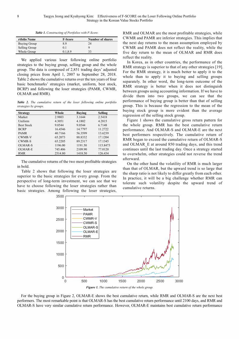
Figure 1 shows the cumulative gross return pattern for
the whole group. RMR has the best cumulative return
performance. And OLMAR-S and OLMAR-E are the next
best performers respectively. The cumulative return of
RMR began to exceed the cumulative return of OLMAR-S
and OLMAR_E at around 850 trading days, and this trend
continues until the last trading day. Once a strategy started
to overwhelm, other strategies could not reverse the trend
afterward.
On the other hand the volatility of RMR is much larger
than that of OLMAR, but the upward trend is so large that
the sharp ratio is not likely to differ greatly from each other.
In practice, it will be a big challenge whether RMR can
tolerate such volatility despite the upward trend of
cumulative returns.
Figure 1. The cumulative return of the whole group.
For the buying group in Figure 2, OLMAR-E shows the best cumulative return, while RMR and OLMAR-S are the next best
performers. The most remarkable point is that OLMAR-S has the best cumulative return performance until 2100 days, and RMR and
OLMAR-S have very similar cumulative return performance. However, OLMAR-E maintains best cumulative return performance
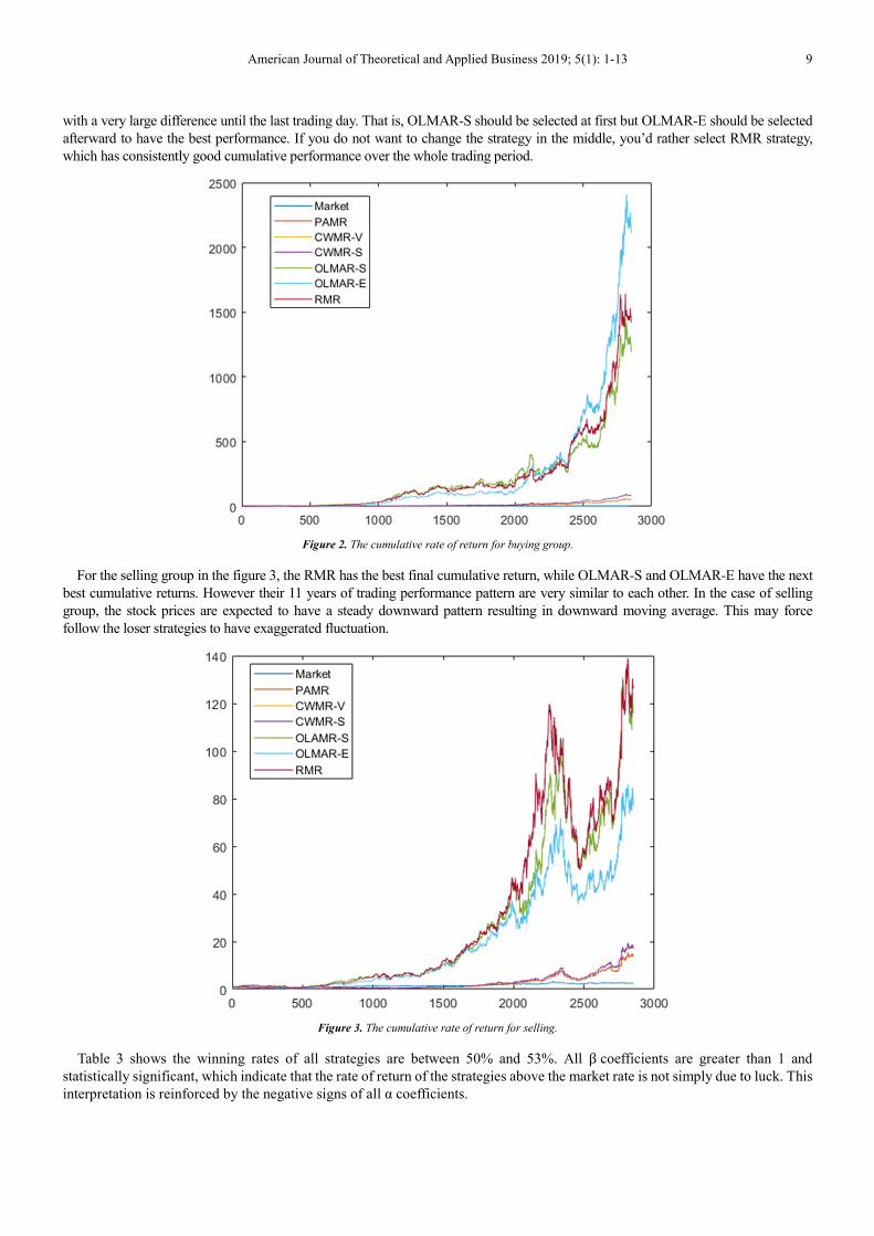
American Journal of Theoretical and Applied Business 2019; 5(1): 1-13 9
with a very large difference until the last trading day. That is, OLMAR-S should be selected at first but OLMAR-E should be selected
afterward to have the best performance. If you do not want to change the strategy in the middle, you’d rather select RMR strategy,
which has consistently good cumulative performance over the whole trading period.
Figure 2. The cumulative rate of return for buying group.
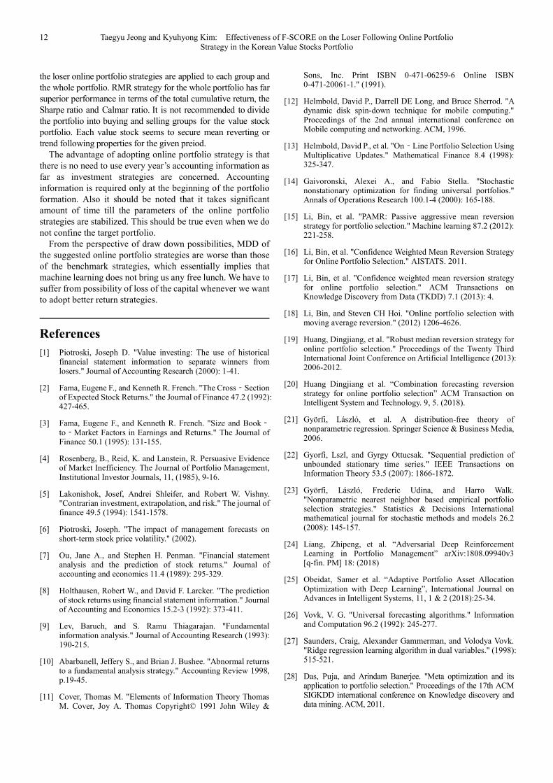
For the selling group in the figure 3, the RMR has the best final cumulative return, while OLMAR-S and OLMAR-E have the next
best cumulative returns. However their 11 years of trading performance pattern are very similar to each other. In the case of selling
group, the stock prices are expected to have a steady downward pattern resulting in downward moving average. This may force
follow the loser strategies to have exaggerated fluctuation.
Figure 3. The cumulative rate of return for selling.
Table 3 shows the winning rates of all strategies are between 50% and 53%. All βcoefficients are greater than 1 and
statistically significant, which indicate that the rate of return of the strategies above the market rate is not simply due to luck. This
interpretation is reinforced by the negative signs of all α coefficients.

10 Taegyu Jeong and Kyuhyong Kim: Effectiveness of F-SCORE on the Loser Following Online Portfolio
Strategy in the Korean Value Stocks Portfolio
Table 3. The regression on the performance of each strategy.
Features Buying Group Selling Group Whole Group
Total trading days 2851 2851 2851
The market average return (Benchmark) 0.00111 0.000892 0.001045
PAMR average return 0.019768 0.004779 0.014282
PAMR winning rate 0.531042 0.508593 0.53946 β1 9.499396 4.037767 7.272506
α1 -14.3057 -4.29594 -10.4799
T-Statistics1 49.35281 78.31946 49.14247
ρ−Value1 0.00 0.00 0.00
CWMR-V average return 0.031159 0.006005 0.022872
CWMR-V winning rate 0.537355 0.509295 0.543669 β2 14.10343 4.938937 10.90435
α2 -21.7435 -5.2506 -16.0479
T-Statistics2 45.663 73.16106 45.84819
ρ−Value2 0.00 0.00 0.00
CWMR-S average return 0.031298 0.00601 0.022876
CWMR-S winning rate 0.537355 0.509295 0.543669 β3 14.16349 4.938718 10.89656
α3 -21.8393 -5.25042 -16.0343
T-Statistics3 45.64476 73.0806 45.81434
ρ−Value3 0.00 0.00 0.00
OLMAR-S average return 0.417924 0.040634 0.419502
OLMAR-S winning rate 0.525079 0.507892 0.535251 β4 196.9162 49.50736 242.1685
α4 -299.186 -53.7872 -359.704
T-Statistics4 45.59244 126.3328 59.81326
ρ−Value4 0.00 0.00 0.00
OLMAR-E average returm 0.740056 0.027012 0.261454
OLMAR-E winning rate 0.531743 0.50228 0.537005 β5 258.1571 33.94083 101.7783
α5 -415.855 -35.6815 -146.589
T-Statistics5 32.42573 150.2631 39.58982
ρ−Value5 0.00 0.00 0.00
RMR average returm 0.497545 0.044347 0.882076
RMR winning rate 0.529639 0.512101 0.537706 β6 208.6969 55.76158 458.3175
α6 -319.4 -61.0716 -732.053
T-Statistics6 38.97511 136.136 53.67906
ρ−Value6 0.00 0.00 0.00
Independent variable is market index rate of return, the
six dependent variables are the rate of return of each of
the six strategies. t-statistic for beta is not reported.
However every beta show the value that is greater than 1,
which implies that results are not just out of luck.
Figure 4 shows that the six loser following strategies
have relatively higher volatility than the rest four
benchmark strategies. This suggests that the higher return
pattern that is possible by active portfolio strategies is
accompanied by higher volatilities. The volatility of the six
loser following strategies are at a similar level with no
significant difference may imply that we may have to
choose the strategy that shows highest cumulative return
performance.
MDDs for the 10 strategies are shown in Figure 5. We see
that the MDD of the buying group is lower than that of the other
groups. The figure clearly shows that we have to suffer from
high Maximum draw down possibilities if we want to have
higher cumulative rate of return. In addition, selling group has
higher drawdown possibilities than other groups. And it would
be a better idea to limit our portfolio to buying group only if we
do not want to suffer from maximum draw down.
Figure 4. Volatility.

American Journal of Theoretical and Applied Business 2019; 5(1): 1-13 11
Figure 5. MDD.
Figure 6 shows the Sharpe ratios for the 10 strategies, where
return and risk are considered simultaneously. OLMAR-E has
the highest Sharpe ratio in the buying group, RMR has the
next. The RMR shows the highest Sharp ratio in the selling as
well as the whole group, OLMAR-S has the next. CWMRs
show poor Sharpe ratios. We have seen that RMR and
OLMAR have very good cumulative rate of return patterns in
Figure 1, and that they have high volatility. Sharpe ratio shows
that risk taking through OLMAR and RMR are very good
strategies when the return is considered together with risk.
Figure 6. Sharpe Ratio.
Figure 7 shows the Calmar ratio, which is very similar to
the Sharpe ratio results in Figure 4. OLMAR-E shows the
highest rate of Calmar in the buying group, OLMAR-S shows
the next. The RMR shows the highest Calmar in the selling
group as well as the whole group, OMMAR-S is the next.
Empirically, RMR and OLMAR show good Calmar ratio
regardless of the portfolio groups.
Figure 7. Calmar Ratio.
So far, we have seen that the RMR strategy for the entire
group is far superior to those the two groups. We used
accounting information at the beginning of the portfolio
formation according to Piostroski’s methodology. For the rest
of the period we do not need accounting information.
In order to apply the results of this paper in practice, we
should consider the transaction costs of daily portfolio
adjustment and the possibility of leveraging when high returns
are expected. We would like to leave the two possibility as a
subject for next research.
From the observations above, we may conclude that it is
worthwhile to adopt active loser following strategies. And
from among active lose following strategies, we may choose
either RMR or OLMAR strategies. In addition we have to
consider the fact that it takes at least 5 years to let the
parameters in the model to settle down and usable in later
periods.
5. Conclusion
For a value stock portfolio, Piotroski’s F-SCORE is used to
construct buying stock group and selling stock group. Six follow
12 Taegyu Jeong and Kyuhyong Kim: Effectiveness of F-SCORE on the Loser Following Online Portfolio
Strategy in the Korean Value Stocks Portfolio
the loser online portfolio strategies are applied to each group and
the whole portfolio. RMR strategy for the whole portfolio has far
superior performance in terms of the total cumulative return, the
Sharpe ratio and Calmar ratio. It is not recommended to divide
the portfolio into buying and selling groups for the value stock
portfolio. Each value stock seems to secure mean reverting or
trend following properties for the given preiod.
The advantage of adopting online portfolio strategy is that
there is no need to use every year’s accounting information as
far as investment strategies are concerned. Accounting
information is required only at the beginning of the portfolio
formation. Also it should be noted that it takes significant
amount of time till the parameters of the online portfolio
strategies are stabilized. This should be true even when we do
not confine the target portfolio.
From the perspective of draw down possibilities, MDD of
the suggested online portfolio strategies are worse than those
of the benchmark strategies, which essentially implies that
machine learning does not bring us any free lunch. We have to
suffer from possibility of loss of the capital whenever we want
to adopt better return strategies.
References
[1] Piotroski, Joseph D. "Value investing: The use of historical financial statement information to separate winners from losers." Journal of Accounting Research (2000): 1-41.
[2] Fama, Eugene F., and Kenneth R. French. "The Cross‐Section of Expected Stock Returns." the Journal of Finance 47.2 (1992): 427-465.
[3] Fama, Eugene F., and Kenneth R. French. "Size and Book‐to‐Market Factors in Earnings and Returns." The Journal of Finance 50.1 (1995): 131-155.
[4] Rosenberg, B., Reid, K. and Lanstein, R. Persuasive Evidence of Market Inefficiency. The Journal of Portfolio Management, Institutional Investor Journals, 11, (1985), 9-16.
[5] Lakonishok, Josef, Andrei Shleifer, and Robert W. Vishny. "Contrarian investment, extrapolation, and risk." The journal of finance 49.5 (1994): 1541-1578.
[6] Piotroski, Joseph. "The impact of management forecasts on short-term stock price volatility." (2002).
[7] Ou, Jane A., and Stephen H. Penman. "Financial statement analysis and the prediction of stock returns." Journal of accounting and economics 11.4 (1989): 295-329.
[8] Holthausen, Robert W., and David F. Larcker. "The prediction of stock returns using financial statement information." Journal of Accounting and Economics 15.2-3 (1992): 373-411.
[9] Lev, Baruch, and S. Ramu Thiagarajan. "Fundamental information analysis." Journal of Accounting Research (1993): 190-215.
[10] Abarbanell, Jeffery S., and Brian J. Bushee. "Abnormal returns to a fundamental analysis strategy." Accounting Review 1998, p.19-45.
[11] Cover, Thomas M. "Elements of Information Theory Thomas M. Cover, Joy A. Thomas Copyright© 1991 John Wiley &
Sons, Inc. Print ISBN 0-471-06259-6 Online ISBN 0-471-20061-1." (1991).
[12] Helmbold, David P., Darrell DE Long, and Bruce Sherrod. "A dynamic disk spin-down technique for mobile computing." Proceedings of the 2nd annual international conference on Mobile computing and networking. ACM, 1996.
[13] Helmbold, David P., et al. "On‐Line Portfolio Selection Using Multiplicative Updates." Mathematical Finance 8.4 (1998): 325-347.
[14] Gaivoronski, Alexei A., and Fabio Stella. "Stochastic nonstationary optimization for finding universal portfolios." Annals of Operations Research 100.1-4 (2000): 165-188.
[15] Li, Bin, et al. "PAMR: Passive aggressive mean reversion strategy for portfolio selection." Machine learning 87.2 (2012): 221-258.
[16] Li, Bin, et al. "Confidence Weighted Mean Reversion Strategy for Online Portfolio Selection." AISTATS. 2011.
[17] Li, Bin, et al. "Confidence weighted mean reversion strategy for online portfolio selection." ACM Transactions on Knowledge Discovery from Data (TKDD) 7.1 (2013): 4.
[18] Li, Bin, and Steven CH Hoi. "Online portfolio selection with moving average reversion." (2012) 1206-4626.
[19] Huang, Dingjiang, et al. "Robust median reversion strategy for online portfolio selection." Proceedings of the Twenty Third International Joint Conference on Artificial Intelligence (2013): 2006-2012.
[20] Huang Dingjiang et al. “Combination forecasting reversion strategy for online portfolio selection” ACM Transaction on Intelligent System and Technology. 9, 5. (2018).
[21] Györfi, László, et al. A distribution-free theory of nonparametric regression. Springer Science & Business Media, 2006.
[22] Gyorfi, Lszl, and Gyrgy Ottucsak. "Sequential prediction of unbounded stationary time series." IEEE Transactions on Information Theory 53.5 (2007): 1866-1872.
[23] Györfi, László, Frederic Udina, and Harro Walk. "Nonparametric nearest neighbor based empirical portfolio selection strategies." Statistics & Decisions International mathematical journal for stochastic methods and models 26.2 (2008): 145-157.
[24] Liang, Zhipeng, et al. “Adversarial Deep Reinforcement Learning in Portfolio Management” arXiv:1808.09940v3 [q-fin. PM] 18: (2018)
[25] Obeidat, Samer et al. “Adaptive Portfolio Asset Allocation Optimization with Deep Learning”, International Journal on Advances in Intelligent Systems, 11, 1 & 2 (2018):25-34.
[26] Vovk, V. G. "Universal forecasting algorithms." Information and Computation 96.2 (1992): 245-277.
[27] Saunders, Craig, Alexander Gammerman, and Volodya Vovk. "Ridge regression learning algorithm in dual variables." (1998): 515-521.
[28] Das, Puja, and Arindam Banerjee. "Meta optimization and its application to portfolio selection." Proceedings of the 17th ACM SIGKDD international conference on Knowledge discovery and data mining. ACM, 2011.
American Journal of Theoretical and Applied Business 2019; 5(1): 1-13 13
[29] Vovk, Volodya, and Chris Watkins. "Universal portfolio selection." Proceedings of the eleventh annual conference on Computational learning theory. ACM, pp.1998.
[30] Sloan, R. "Do stock prices fully reflect information in accruals and cash flows about future earnings? (Digest summary)." Accounting review 71.3 (1996): 289-315.
[31] Sweeny, A. "Debt-Covenant Violations and Managers' Accounting Responses." Journal of Accounting and Economics 17 (1994): 281-308.
[32] Myers, Stewart C., and Nicholas S. Majluf. "Corporate Financing and Investment Decisions When Firms Have Information That Investors Do Not Have." Journal of Financial Economics 13.2 (1984): 187-221.
[33] Miller, M., and K. Rock. "Dividend Policy under Asymmetric Information." Journal of Finance 40 (1985): 1031-1051.
[34] Bondt, Werner FM, and Richard Thaler. "Does the stock market overreact" The Journal of finance 40.3 (1985): 793-805.
[35] Poterba, James M., and Lawrence H. Summers. "Mean reversion in stock prices: Evidence and implications." Journal of financial economics 22.1 (1988):27-59.
[36] Lo, Andrew W., and A. Craig MacKinlay. "When are contrarian
profits due to stock market overreaction." Review of Financial studies 3.2 (1990): 175-205.
[37] Borodin, Oleg, et al. "Molecular dynamics study of the influence of solid interfaces on poly (ethylene oxide) structure and dynamics." Macromolecules 36.20, 2003, p.7873-7883.
[38] Borodin, Allan, Ran El-Yaniv, and Vincent Gogan. "Can We Learn to Beat the Best Stock." J. Artif. Intell. Res. (JAIR) 21 (2004, 579-594.
[39] Duchi, John, et al. "Efficient projections onto the l 1-ball for learning in high dimensions." Proceedings of the 25th international conference on Machine learning. ACM, 2008.
[40] Sharpe, William F. "Capital asset prices: A theory of market equilibrium under conditions of risk." The journal of finance 19.3 (1964): 425-442.
[41] Sharpe, William F. "The sharpe ratio." Journal of portfolio management 21.1 (1994): 49-58.
[42] Magdon-Ismail, Malik, et al. "On the maximum drawdown of a Brownian motion." Journal of applied probability 41.1 (2004): 147-161.
[43] Kahn, R., and R. Grinold. "Active Portfolio Management." New York, NY: McGraw-Hil1 (1999).