Effective Methods to Tackle the Equivalent Mutant...
195
Effective Methods to Tackle the Equivalent Mutant Problem when Testing Software with Mutation Marinos Kintis A thesis submitted in fulfilment of the requirements for the degree of Doctor of Philosophy of the Athens University of Economics and Business Department of Informatics Athens University of Economics and Business June 2016
Transcript of Effective Methods to Tackle the Equivalent Mutant...
Effective Methods to Tackle the EquivalentMutant Problem when Testing Software with
Mutation
Marinos Kintis
A thesis submitted in fulfilment of the
requirements for the degree of
Doctor of Philosophy
of the
Athens University of Economics and Business
Department of Informatics
Athens University of Economics and Business
June 2016

c© 2016 Marinos Kintis

Abstract
Mutation Testing is undoubtedly one of the most effective software testing tech-
niques that has been applied to different software artefacts at different testing levels.
Apart from mutation’s versatility, its most important characteristic is its ability to
detect real faults. Unfortunately, mutation’s adoption in practice is inhibited, pri-
marily due to the manual effort involved in its application. This effort is attributed
to the Equivalent Mutant Problem.
The Equivalent Mutant Problem is a well-known impediment to mutation’s
practical adoption that affects all phases of its application. To exacerbate the sit-
uation, the Equivalent Mutant Problem has been shown to be undecidable in its
general form. Thus, no complete, automated solution exists. Although previous re-
search has attempted to address this problem, its circumvention remains largely an
open issue. This thesis argues that effective techniques that considerably ameliorate
the problem’s adverse effects can be devised. To this end, the thesis introduces and
empirically evaluates several such approaches that are based on Mutant Classifica-
tion, Static Analysis and Code Similarity.
First, the thesis proposes a novel mutant classification technique, named Isolat-
ing Equivalent Mutants (I-EQM) classifier, whose salient feature is the utilisation of
second order mutants to automatically isolate first order equivalent ones. The em-
pirical evaluation of the approach, based on real-world test subjects, suggests that
I-EQM outperforms the existing techniques and results in a more effective testing
process.
Second, the thesis formally defines nine data flow patterns that can automati-
cally detect equivalent and partially equivalent mutants. Their empirical evaluation

Abstract 4
corroborates this statement, providing evidence of their existence in real-world soft-
ware and their equivalent mutant detection capabilities.
Third, MEDIC (Mutants’ Equivalence Discovery), an automated framework
that implements the aforementioned patterns and manages to detect equivalent and
partially equivalent mutants in different programming languages, is introduced. The
experimental investigation of the tool, based on a large set of manually analysed
mutants, reveals that MEDIC can detect efficiently more than half of the considered
equivalent mutants and provides evidence of automated stubborn mutant detection.
Finally, the thesis proposes the concept of mirrored mutants, that is mutants af-
fecting similar code fragments and, more precisely, analogous code locations within
these fragments. It is postulated that mirrored mutants exhibit analogous behaviour
with respect to their equivalence. The empirical evaluation of this concept supports
this statement and suggests that the number of the equivalent mirrored mutants that
have to be manually analysed can be reduced approximately by half.

To my family

Acknowledgements
First of all, I would like to thank my supervisor, Prof. Nicos Malevris, for his
guidance, tireless support and for sharing his time and knowledge with me. I would
also like to thank my co-supervisors, Prof. Emmanouil Giakoumakis and Prof.
Yannis Kotidis, for their advice, encouragement and constructive suggestions.
I am particularly grateful to Prof. Panos Constantopoulos for his counsel and
kind support and to Prof. Ion Androutsopoulos, Prof. Maria Virvou and Prof. Em-
manuel Yannakoudakis for taking the time to be on my defence committee and for
their insightful comments.
My sincere thanks go to Mike Papadakis for his assistance and our endless
discussions and Matthew Patrick and Yue Jia for their positive advice. I would also
like to thank Vassilis Zafeiris and Nikos Diamantidis for their generous help during
my studies.
Many thanks go to my colleagues at the Information Systems and Databases
Laboratory and the Department of Informatics for their support and fruitful discus-
sions. I would also like to thank the anonymous reviewers of my submitted papers
for their helpful comments and valuable feedback.
I particularly appreciated working with several exceptional undergraduate
and postgraduate students, including Andreas Papadopoulos, Evaggelos Valvis,
Maria Markaki, Ioannis Babakas, Sotiria Giannitsari, Makrina Polydorou, Foivos
Anagnou-Misyris, Loukas-Pavlos Basios, Nikolaos Panagopoulos and Dimitrios
Spiliotis.
I gratefully acknowledge financial support for my studies from Empirikion
Foundation, AUEB’s Basic Research Funding Program (BRFP) 3 and RC AUEB.

Acknowledgements 7
Finally, I would like to express my deepest gratitude to my fiancee and my
family who continuously supported me throughout this difficult journey.

Contents
1 Introduction 16
1.1 Context of the Thesis: Mutation Testing . . . . . . . . . . . . . . . 17
1.1.1 Mutation Testing: An Example . . . . . . . . . . . . . . . . 18
1.2 Motivation . . . . . . . . . . . . . . . . . . . . . . . . . . . . . . . 20
1.2.1 Mutation’s Effectiveness: Fault Detection . . . . . . . . . . 20
1.2.2 Mutation’s Manual Cost: An Open Issue . . . . . . . . . . 21
1.3 Scope of the Thesis . . . . . . . . . . . . . . . . . . . . . . . . . . 22
1.4 Contributions of the Thesis . . . . . . . . . . . . . . . . . . . . . . 23
1.5 Organisation of the Thesis . . . . . . . . . . . . . . . . . . . . . . 24
2 Mutation Testing: Background and Cost-Reduction Techniques 27
2.1 General Infomation . . . . . . . . . . . . . . . . . . . . . . . . . . 27
2.1.1 Underlying Principles . . . . . . . . . . . . . . . . . . . . 28
2.1.2 The Mutation Analysis Process . . . . . . . . . . . . . . . 30
2.1.3 Mutation’s Cost . . . . . . . . . . . . . . . . . . . . . . . . 32
2.1.4 The Equivalent Mutant Problem . . . . . . . . . . . . . . . 34
2.2 Manual Analysis of Equivalent Mutants . . . . . . . . . . . . . . . 35
2.3 Cost-Reduction Techniques . . . . . . . . . . . . . . . . . . . . . . 36
2.3.1 Tackling the Equivalent Mutant Problem . . . . . . . . . . 37
2.3.2 Reducing Mutation’s Computational Cost . . . . . . . . . . 41
2.4 Summary . . . . . . . . . . . . . . . . . . . . . . . . . . . . . . . 45
3 Equivalent Mutant Isolation via Higher Order Mutation 47
3.1 Background . . . . . . . . . . . . . . . . . . . . . . . . . . . . . . 49

Contents 9
3.1.1 Mutants’ Impact . . . . . . . . . . . . . . . . . . . . . . . 49
3.1.2 Mutation Analysis using Mutant Classifiers . . . . . . . . . 50
3.2 First Order Mutant Classification via Second Order Mutation . . . . 54
3.2.1 HOM Classifier: Mutant Classification Process . . . . . . . 55
3.2.2 Isolating Equivalent Mutants (I-EQM) Classifier . . . . . . 59
3.3 Empirical Study . . . . . . . . . . . . . . . . . . . . . . . . . . . . 60
3.3.1 Research Questions . . . . . . . . . . . . . . . . . . . . . . 60
3.3.2 Subject Programs and Supporting Tool . . . . . . . . . . . 61
3.3.3 Benchmark Mutant Sets . . . . . . . . . . . . . . . . . . . 62
3.3.4 Experimental Setup . . . . . . . . . . . . . . . . . . . . . . 64
3.4 Empirical Findings . . . . . . . . . . . . . . . . . . . . . . . . . . 67
3.4.1 RQ 3.1 and RQ 3.2: Precision and Recall . . . . . . . . . . 67
3.4.2 RQ 3.1 and RQ 3.2: Accuracy and Fβ scores . . . . . . . . 73
3.4.3 RQ 3.3: Classifiers’ Stability . . . . . . . . . . . . . . . . . 75
3.4.4 Statistical Analysis . . . . . . . . . . . . . . . . . . . . . . 76
3.4.5 Discussion . . . . . . . . . . . . . . . . . . . . . . . . . . 78
3.4.6 Mutants with Higher Impact . . . . . . . . . . . . . . . . . 79
3.4.7 Threats to Validity . . . . . . . . . . . . . . . . . . . . . . 82
3.5 Summary . . . . . . . . . . . . . . . . . . . . . . . . . . . . . . . 84
4 Equivalent Mutant Detection via Data Flow Patterns 86
4.1 Background . . . . . . . . . . . . . . . . . . . . . . . . . . . . . . 87
4.1.1 Employed Mutation Operators . . . . . . . . . . . . . . . . 87
4.1.2 Static Single Assignment (SSA) Form . . . . . . . . . . . . 89
4.2 Equivalent Mutants and Data Flow Analysis . . . . . . . . . . . . . 90
4.2.1 Function Definitions . . . . . . . . . . . . . . . . . . . . . 91
4.2.2 Use-Def (UD) and Use-Ret (UR) Categories of Patterns . . 94
4.2.3 Def-Def (DD) and Def-Ret (DR) Categories of Patterns . . . 102
4.3 Empirical Study and Results . . . . . . . . . . . . . . . . . . . . . 106
4.3.1 Experimental Setup . . . . . . . . . . . . . . . . . . . . . . 106
4.3.2 Empirical Findings . . . . . . . . . . . . . . . . . . . . . . 107

Contents 10
4.4 Summary . . . . . . . . . . . . . . . . . . . . . . . . . . . . . . . 109
5 A Static Analysis Framework for Equivalent Mutant Identification 110
5.1 Background: Problematic Data Flow Patterns . . . . . . . . . . . . 111
5.1.1 Use-Def (UD) Category of Patterns . . . . . . . . . . . . . 112
5.1.2 Use-Ret (UR) Category of Patterns . . . . . . . . . . . . . 116
5.1.3 Def-Def (DD) Category of Patterns . . . . . . . . . . . . . 118
5.1.4 Def-Ret (DR) Category of Patterns . . . . . . . . . . . . . . 120
5.2 MEDIC – Mutants’ Equivalence DIsCovery . . . . . . . . . . . . . 122
5.2.1 T. J. Watson Libraries for Analysis (WALA) . . . . . . . . . 122
5.2.2 MEDIC’s Implementation Details . . . . . . . . . . . . . . 123
5.3 Empirical Study . . . . . . . . . . . . . . . . . . . . . . . . . . . . 130
5.3.1 Research Questions . . . . . . . . . . . . . . . . . . . . . . 131
5.3.2 Experimental Procedure . . . . . . . . . . . . . . . . . . . 131
5.4 Empirical Findings . . . . . . . . . . . . . . . . . . . . . . . . . . 137
5.4.1 RQ 5.1: MEDIC’s Effectiveness and Efficiency . . . . . . . 137
5.4.2 RQ 5.2: Equivalent Mutant Detection in Different Program-
ming Languages . . . . . . . . . . . . . . . . . . . . . . . 141
5.4.3 RQ 5.3: Partially Equivalent Mutants’ Killability . . . . . . 142
5.4.4 Threats to Validity . . . . . . . . . . . . . . . . . . . . . . 144
5.5 Summary . . . . . . . . . . . . . . . . . . . . . . . . . . . . . . . 145
6 Eliminating Equivalent Mutants via Code Similarity 148
6.1 Background: Code Similarity . . . . . . . . . . . . . . . . . . . . . 149
6.2 Mirrored Mutants . . . . . . . . . . . . . . . . . . . . . . . . . . . 151
6.2.1 Mirrored Mutants: Definition . . . . . . . . . . . . . . . . 151
6.2.2 Mirrored Mutants and Equivalent Mutant Discovery . . . . 154
6.3 Empirical Study and Results . . . . . . . . . . . . . . . . . . . . . 155
6.3.1 Research Questions . . . . . . . . . . . . . . . . . . . . . . 155
6.3.2 Experimental Study . . . . . . . . . . . . . . . . . . . . . 156
6.3.3 Experimental Results . . . . . . . . . . . . . . . . . . . . . 162

Contents 11
6.3.4 Threats to Validity . . . . . . . . . . . . . . . . . . . . . . 164
6.4 Summary . . . . . . . . . . . . . . . . . . . . . . . . . . . . . . . 165
7 Conclusions and Future Work 167
Appendices 172
A Publications 172
A.1 Refereed Journal Papers . . . . . . . . . . . . . . . . . . . . . . 172
A.2 Refereed Conference and Workshop Papers . . . . . . . . . . . . 172
Bibliography 174

List of Figures
1.1 Examples of Killable and Equivalent Mutants . . . . . . . . . . . . 19
2.1 Example of a Second Order Mutant . . . . . . . . . . . . . . . . . 30
2.2 Mutation Analysis Process . . . . . . . . . . . . . . . . . . . . . . 31
3.1 Mutation Analysis using Mutant Classifiers . . . . . . . . . . . . . 51
3.2 HOM Classifier’s Hypothesis . . . . . . . . . . . . . . . . . . . . . 56
3.3 Mutant Classifiers’ Comparison: Control Mutant Set 1 . . . . . . . 73
3.4 Mutant Classifiers’ Comparison: Control Mutant Set 2 . . . . . . . 74
3.5 Mutant Classifiers’ Comparison: Control Mutant Sets 1+2 . . . . . 75
3.6 Classifiers’ Stability . . . . . . . . . . . . . . . . . . . . . . . . . . 76
3.7 Variation of the Effectiveness Measures . . . . . . . . . . . . . . . 77
3.8 Coverage Impact Classifier: Higher Impact Values . . . . . . . . . . 81
3.9 HOM Classifier: Higher Impact Values . . . . . . . . . . . . . . . . 81
3.10 Differences between Studied Control Mutant Sets . . . . . . . . . . 82
4.1 Static Single Assignment Form Example . . . . . . . . . . . . . . . 90
4.2 Source Code of the Bisect test subject . . . . . . . . . . . . . . . 95
5.1 SSA Representation Example (generated by WALA) . . . . . . . . 113
5.2 Problematic Situations Detected by the Use-Def Category of Patterns 115
5.3 Problematic Situations Detected by the Use-Ret Category of Patterns 117
5.4 Problematic Situations Detected by the Def-Def Category of Patterns 119
5.5 SameBB-DR Pattern: Handling Non-local Variables . . . . . . . . . 121
5.6 MEDIC’s Data Model . . . . . . . . . . . . . . . . . . . . . . . . . 125
5.7 Example Cypher Query . . . . . . . . . . . . . . . . . . . . . . . . 127

List of Figures 13
5.8 SameLine-UD Pattern: Instantiation of MEDIC’s Generic Algorithm 129
5.9 Equivalent Mutants per Mutation Operator . . . . . . . . . . . . . . 133
5.10 MEDIC’s Application Process . . . . . . . . . . . . . . . . . . . . 134
5.11 Automatically Identified Equivalent Mutants per Mutation Operator 139
5.12 Venn Diagram: Relation between PE and K, E and S Mutant Sets . . 143
6.1 Source Code of the Triangle test subject. . . . . . . . . . . . . . 152
6.2 Examples of Mirrored Mutants . . . . . . . . . . . . . . . . . . . . 153
6.3 Generating a Random Sample of Mirrored Mutants . . . . . . . . . 159

List of Tables
2.1 Mutation Operators for FORTRAN 77 programs . . . . . . . . . . . 28
2.2 Causes of Mutants’ Equivalence . . . . . . . . . . . . . . . . . . . 36
3.1 I-EQM Evaluation: Subject Program Details . . . . . . . . . . . . . 61
3.2 JAVALANCHE’s Mutation Operators . . . . . . . . . . . . . . . . . 62
3.3 Control Mutant Sets’ Profile w.r.t. Subject Programs . . . . . . . . 63
3.4 Control Mutant Sets’ Profile w.r.t. Mutation Operators . . . . . . . 64
3.5 Mutant Classification using the Coverage Impact Classifier . . . . . 68
3.6 Mutant Classification using the HOM Classifier: Control Set 1 . . . 68
3.7 Mutant Classification using the HOM Classifier: Control Set 2 . . . 69
3.8 Mutant Classification using the I-EQM Classifier: Control Set 1 . . 70
3.9 Mutant Classification using the I-EQM Classifier: Control Set 2 . . 70
3.10 Mutant Classification using the Coverage Impact Classifier: Sets 1+2 72
3.11 Mutant Classification using the I-EQM Classifier: Sets 1+2 . . . . . 72
3.12 Statistical Significance based on the Wilcoxon Signed Rank Test . . 78
4.1 Mutation Operators of MUJAVA . . . . . . . . . . . . . . . . . . . . 88
4.2 Data Flow Patterns’ Evaluation: Subject Program Details . . . . . . 107
4.3 Data Flow Patterns’ Detection Power . . . . . . . . . . . . . . . . . 108
5.1 MEDIC’s Evaluation: Java Test Subjects’ Details . . . . . . . . . . 132
5.2 MEDIC’s Evaluation: JavaScript Test Subjects’ Details . . . . . . . 135
5.3 Automatically Identified Equivalent Mutants per Java Test Subject . 138
5.4 Equivalent Mutant Detection Run-time . . . . . . . . . . . . . . . . 140
5.5 Automatically Identified Equiv. Mutants per JavaScript Test Subject 141
List of Tables 15
5.6 Automatically Identified Part. Equiv. Mutants per JavaScript Program141
5.7 Partially Equivalent Mutants’ Killability . . . . . . . . . . . . . . . 142
6.1 Mirrored Mutants’ Evaluation: Test Subjects’ Details . . . . . . . . 158
6.2 Randomly Selected Mirrored Mutants’ Details . . . . . . . . . . . . 159
6.3 Manual Analysis of Mirrored Mutants . . . . . . . . . . . . . . . . 160
6.4 Mirrored Mutants: Experimental Results . . . . . . . . . . . . . . . 163
6.5 Mirrored Mutants: Cost Reduction . . . . . . . . . . . . . . . . . . 164
Chapter 1
Introduction
Among the various software development phases, testing typically accounts for
more than 50% of total development costs, even more for safety-critical applica-
tions [1–3]. Despite this fact, testing constitutes an invaluable activity of software
development: it provides a systematic way of uncovering software faults, and, thus,
increases the practitioners’ confidence in the software’s correctness.
Software testing utilises formal coverage criteria to guide the testing process.
These criteria require specific elements of the artefact under test, called test require-
ments, to be covered or satisfied by test cases [3]. For instance, statement coverage
requires all statements of the source code of the program under test to be covered
by at least one test case and branch coverage necessitates covering all branches of
the program’s control flow graph.
In other words, coverage criteria constitute a means of distinguishing between
test cases that possess a specific property and ones that do not and, thus, guide the
testing process towards those particular test cases. Additionally, they can act as
stopping rules for the testing process [3].
Unfortunately, covering certain coverage criteria is quite demanding in terms
of computational resources and, more importantly, human effort. There are three
main reasons for this problem:
1. Various coverage criteria impose a vast number of test requirements.
2. The generation of appropriate test cases that cover the imposed test require-
ments is a difficult task that cannot be automated in its entirety.

1.1. Context of the Thesis: Mutation Testing 17
3. Infeasible test requirements, i.e. test requirements that cannot be covered by
any test case, require human intervention to be identified.
The present thesis introduces several techniques that attempt to address the
aforementioned shortcomings in the context of mutation testing. The motivation of
such a decision is presented in the next sections, along with an outline of mutation’s
problems and the remedies that this thesis proposes.
1.1 Context of the Thesis: Mutation TestingMutation testing is a very powerful technique for testing software with a rich history
that began in 1971 by a class term paper of Richard Lipton [4]. Mutation has been
increasingly studied since its introduction with several available literature surveys
[5–9] and introductory book chapters [3, 10].
Mutation has a plethora of applications in software testing: it has been utilised
in the context of many programming languages, e.g. FORTRAN [11–13], C [14–
16], Java [17–22], Smalltalk [23], Python [24], Haskell [25], JavaScript [26, 27],
SQL [28–32], and different testing levels, e.g. specification level [33], unit level
[34], integration level [35], system level [36, 37].
Mutation is not restricted to testing program source code, it has also been
applied to other software artefacts, e.g. finite state machines [38, 39], net-
work protocols [40], security policies [41–43], software product lines [44, 45],
databases [28, 46, 47]. Finally, it has been utilised to support many testing activi-
ties, e.g. test case generation [48–55], regression testing [56, 57], fault localisation
[58–60], Graphical User Interface (GUI) testing [61, 62].
Mutation is a fault-based technique: it induces artificial faults to the artefact
under test. These faults, which constitute the imposed test requirements, are called
mutants and are simple syntactic changes that are based on specific rules known as
mutation operators.
The application of mutation entails the generation of the mutants of the evalu-
ated artefact, each one containing one artificial fault, and requires their coverage by
appropriate test cases. If such a test case is found, the mutant is termed killed. In

1.1. Context of the Thesis: Mutation Testing 18
a different situation, it is termed alive. A live mutant can be either a killable or an
equivalent one.
A killable mutant is one that can be killed but the available test cases are inad-
equate for this task, thus, new ones must be created. An equivalent mutant is one
that cannot be killed by any test case, that is an equivalent mutant is semantically
equivalent to the artefact under test despite being syntactically different. Examples
of such mutants are presented in the next section (see Figure 1.1).
For the purposes of this introduction, this succinct description of mutation suf-
fices. All the aforementioned concepts will be revisited and elaborated further in
Chapter 2.
This thesis primarily focuses on program mutation, i.e. the application of mu-
tation testing to the source code of a program under test. In this case, mutants cor-
respond to different versions of this program, which is called the original program,
and their “coverage” to the discovery of appropriate test cases that will differentiate
the behaviour of the mutants from that of the original program.
1.1.1 Mutation Testing: An Example
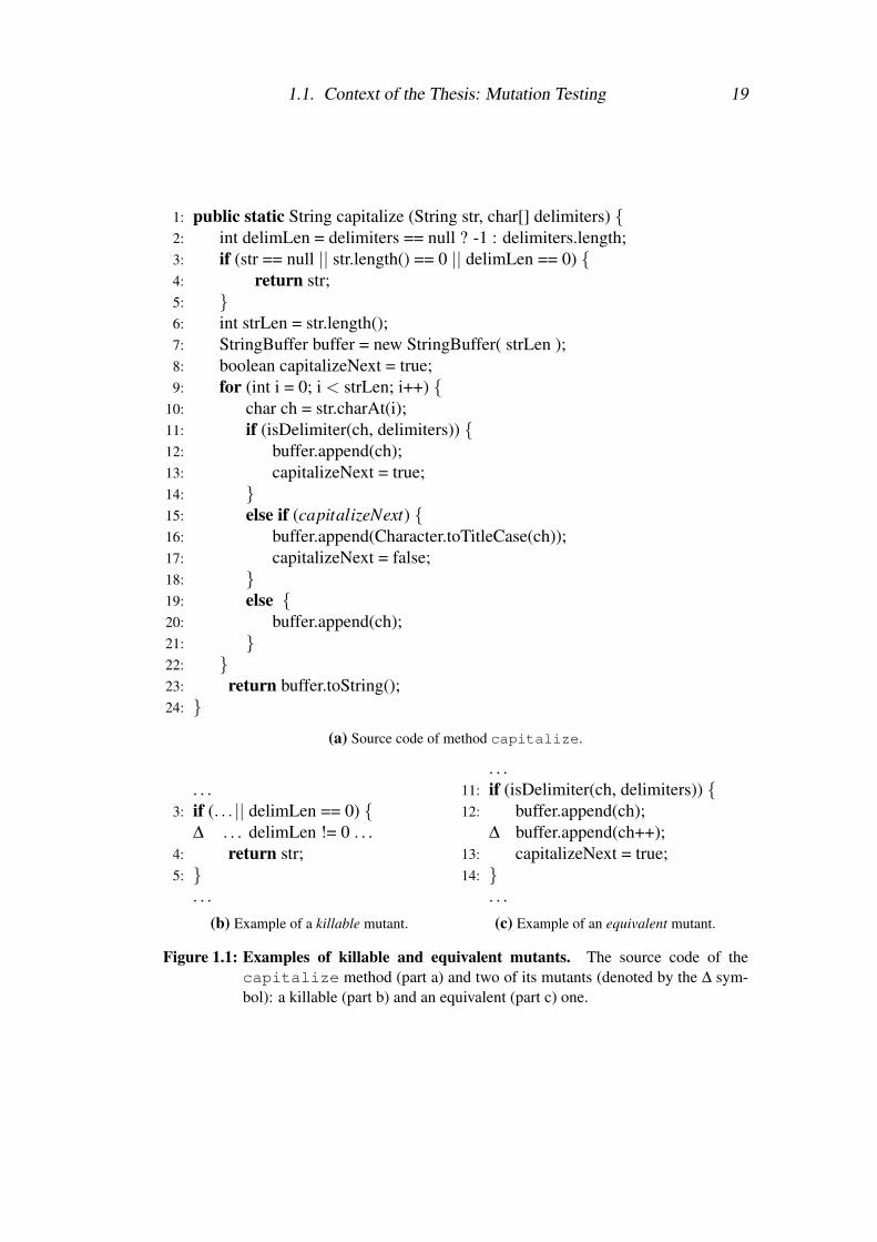
An illustrative example of the aforementioned concepts is depicted in Figure 1.1.
The figure presents the source code of the capitalize method1 (Figure 1.1a),
along with two of its mutants (Figure 1.1b and Figure 1.1c). Method capitalize
capitalises all the delimiter-separated words of its first argument; for example,
capitalize("hello world", null) returns Hello World.
Figure 1.1b illustrates the code fragment of a killable mutant, that is a mutant
that can be killed. This particular mutant is generated by the Relational Operator
Replacement (ROR) mutation operator (see Table 4.1 for more details) and affects
the statement of line 3 of the original program. Note that the mutated statement is
denoted by the ∆ symbol in the figure and will replace that of the original program.
After examining the source code of the method, it becomes apparent that this
mutant can be easily killed by non-empty argument values. Indeed, a test case with
1The method belongs to the WordUtils class of the Apache Commons Lang project (https://commons.apache.org).
1.1. Context of the Thesis: Mutation Testing 19
1: public static String capitalize (String str, char[] delimiters) {2: int delimLen = delimiters == null ? -1 : delimiters.length;3: if (str == null || str.length() == 0 || delimLen == 0) {4: return str;5: }6: int strLen = str.length();7: StringBuffer buffer = new StringBuffer( strLen );8: boolean capitalizeNext = true;9: for (int i = 0; i < strLen; i++) {
10: char ch = str.charAt(i);11: if (isDelimiter(ch, delimiters)) {12: buffer.append(ch);13: capitalizeNext = true;14: }15: else if (capitalizeNext) {16: buffer.append(Character.toTitleCase(ch));17: capitalizeNext = false;18: }19: else {20: buffer.append(ch);21: }22: }23: return buffer.toString();24: }
(a) Source code of method capitalize.
. . .3: if (. . . || delimLen == 0) {
∆ . . . delimLen != 0 . . .4: return str;5: }
. . .(b) Example of a killable mutant.
. . .11: if (isDelimiter(ch, delimiters)) {12: buffer.append(ch);
∆ buffer.append(ch++);13: capitalizeNext = true;14: }
. . .(c) Example of an equivalent mutant.
Figure 1.1: Examples of killable and equivalent mutants. The source code of thecapitalize method (part a) and two of its mutants (denoted by the ∆ sym-bol): a killable (part b) and an equivalent (part c) one.

1.2. Motivation 20
str="hello world" and delimiters={ " " } will kill the mutant: the
original program will return Hello World, whereas the mutant hello world.
Figure 1.1c presents an example of another mutant of the method. This mu-
tant is generated by the Arithmetic Operator Insertion Short-cut (AOIS) mutation
operator (see Table 4.1 for more details) and affects line 12 of the original program.
By carefully executing this mutant, it can be concluded that it is an equivalent one:
after the execution of the mutated statement, there is no use of variable ch capable
of revealing the imposed change.
1.2 MotivationFrom the previous sections, it is immediately apparent that mutation is an extremely
versatile technique. It can be applied to different programming languages at differ-
ent testing levels, to either test various software artefacts or support the testing pro-
cess. Although mutation’s flexibility is impressive, its most important characteristic
is its fault-detection capabilities.
1.2.1 Mutation’s Effectiveness: Fault Detection
Mutation’s fundamental premise is that mutants resemble real faults. As coined by
Geist et al. [63]:
“If the software contains a fault, it is likely that there is a mutant that
can only be killed by a test case that also reveals the fault.”
Several research studies have empirically investigated whether this premise
holds [64–68]. More precisely, the findings of Daran and Thevenod-Fosse [64]
indicate that the erroneous program states that are caused by mutants resemble the
ones caused by real faults. The studies of Andrews et al. [65, 66] suggest that
mutants provide a good indication of the fault-detection ability of a test suite.
Do and Rothermel [67] evaluated the use of mutants in the empirical assess-
ment of test case prioritisation techniques and concluded that mutants can provide
practical replacements of hand-seeded faults. Finally, the findings of Just et al. [68]
demonstrate that there is a correlation between a test suite’s mutation score and its
real-fault detection rate.

1.2. Motivation 21
Apart from its fault-detection capabilities, researchers have empirically com-
pared mutation with several coverage criteria, e.g. control flow [69, 70] and data
flow [71–74]. Specifically, Offutt and Voas [69] formally showed that mutation
testing subsumes various control flow coverage criteria. Li et al. [70] compared
mutation with four unit-level coverage criteria and concluded that test suites gener-
ated to cover mutation detected more faults.
Analogous results were obtained in the case of data flow criteria. Several stud-
ies compared mutation testing with the all-uses data flow criterion [75–77], e.g.
[71–74], and suggest that test suites that cover mutation are very close to covering
all-uses and detect more faults.
The aforementioned studies provide corroborating evidence to support muta-
tion’s effectiveness. Their results suggest that test data generated to cover mutation
are of high quality and are effective in detecting real faults, thus, increasing the
practitioners’ confidence in the software’s dependability and robustness.
1.2.2 Mutation’s Manual Cost: An Open Issue
Despite its effectiveness, mutation lacks widespread adoption in practice, with the
main culprit being its cost. Mutation’s cost can be largely attributed to:
1. The vast number of generated mutants.
2. The Equivalent Mutant Problem, i.e. the undesirable consequences caused
by the presence of equivalent mutants.
As discussed later in Chapter 2, mutation generates an enormous number of
mutants by applying the employed mutation operators to all possible source code
locations of the program under test. These mutants require high computational
resources in order to be executed with the available test cases and considerable
human effort in order to be killed. Thus, impairing mutation’s ability to scale to
real-world programs.
To worsen the situation, equivalent mutants cannot be killed, thus, affecting
negatively all phases of the mutation’s application process (see also Section 2.1.4):
(1) equivalent mutants are generated without contributing to the testing process, (2)
1.3. Scope of the Thesis 22
they waste computational resources when executed with test data and (3) substantial
human effort is misspent when attempting to kill them.
Research studies have shown that an equivalent mutant requires approximately
15 minutes of manual analysis in order to be identified [78–80]. Additionally, sev-
eral studies provide evidence that equivalent mutants are harder to detect than in-
feasible test requirements of other coverage criteria, e.g. all-uses [72, 74]. By con-
sidering these facts, along with the vast number of generated mutants, it becomes
clear that the equivalent mutant problem constitutes a major hindrance to mutation’s
practical adoption.
Although researchers have proposed various approaches to manage the number
of generated mutants, e.g. selective mutation [81], weak mutation [82–84], higher
order mutation [85–88], automated techniques to tackle the equivalent mutant prob-
lem are scarce, mainly, due to the problem’s undecidable nature [89].
1.3 Scope of the ThesisFrom the previous sections, it becomes evident that there are several obstacles to be
surmounted before mutation can be widely adopted in practice. This thesis attempts
to tip the scales in favour of mutation by introducing several automated techniques
that reduce the manual effort involved in its application.
Particularly, this thesis investigates ways of ameliorating the adverse effects
of the equivalent mutant problem. To this end, the following questions are investi-
gated:
Q1 Can a considerable number of equivalent mutants be automatically de-
tected?
The equivalent mutant problem, being undecidable in its general form, is only
susceptible to partial solutions. Nevertheless, if a large number of equivalent
mutants can be automatically detected, then the human effort involved in the
application of mutation can be considerably reduced, boosting the technique’s
practical adoption.
Q2 Can mutant classification constitute a viable alternative to mutation?

1.4. Contributions of the Thesis 23
Various researchers have proposed approximation techniques that reduce the
number of the considered equivalent mutants at the cost of the techniques’
effectiveness (cf. Section 2.3.1). Mutant classification techniques are one
such example. Approaches based on mutation classification classify mutants
as possibly equivalent and possibly killable ones and suggest the utilisation of
the resulting possibly killable mutant set for the purposes of mutation testing.
If such approaches can classify most of the killable mutants correctly while
maintaining the number of the misclassified equivalent ones at a reasonably
low level, then their effectiveness will be significantly high and the manual
cost involved in their application will be substantially reduced.
Q3 Can knowledge about the equivalence of the already analysed mutants be
leveraged to identify new equivalent mutants in the presence of software
clones?
Research studies suggest that software systems include cloned code. Thus,
if mutants belonging to software clones exhibit analogous behaviour with re-
spect to their equivalence or killability, then considerable effort savings can
be achieved by automatically classifying mutants based on the equivalence or
killability of the already analysed ones.
1.4 Contributions of the ThesisThe contributions of this dissertation can be summarised in the following points:
1. The introduction of a novel mutant classification technique, termed Higher
Order Mutation (HOM) classifier, that utilises higher order mutants to auto-
matically classify first order ones (Chapter 3).
2. The proposal of a combined mutant classification scheme, named Isolating
Equivalent Mutants (I-EQM), that is synthesised by two mutant classification
approaches and outperforms the previously proposed ones (Chapter 3).
3. The introduction and formal definition of several data flow patterns that can
automatically detect equivalent and partially equivalent mutants (Chapter 4).

1.5. Organisation of the Thesis 24
4. MEDIC, an automated, static analysis tool that can efficiently detect equiv-
alent and partially equivalent mutants in different programming languages
(Chapter 5).
5. An investigation of whether or not mutants belonging to software clones,
termed mirrored mutants, exhibit analogous behaviour with respect to their
equivalence (Chapter 6).
6. An investigation of the relationship between mutants’ impact and mutants’
killability (Chapter 3).
7. An investigation of the relationship among equivalent, partially equivalent
and stubborn mutants (Chapter 5).
8. Experimental results pertaining to the utilisation of mirrored mutants for test
case generation purposes (Chapter 6).
9. A publicly available data set for comparing mutant classifiers (Chapter 3).
10. An empirical study evaluating the effectiveness and stability of various mu-
tant classification techniques (Chapter 3).
11. An empirical study that investigates the detection power of the proposed data
flow patterns and their existence in real-world software (Chapter 4).
12. An empirical study that evaluates the effectiveness, efficiency and cross-
language nature of MEDIC (Chapter 5).
13. An empirical study that examines the usefulness of mirrored mutants in de-
tecting equivalent ones and generating test cases that target other mirrored
mutants (Chapter 6).
1.5 Organisation of the ThesisThe remaining of this thesis is organised as follows:

1.5. Organisation of the Thesis 25
Chapter 2 furnishes a more detailed view of mutation testing. It begins by de-
scribing the two fundamental hypotheses of the approach, along with mutation’s ap-
plication process. Next, it presents the sources of mutation’s cost and the equivalent
mutant problem and continues by discussing the main causes of mutants’ equiva-
lence. Finally, the chapter concludes by describing previous work on the detection
of equivalent mutants, minimum mutant sets and the reduction of mutation’s com-
putational cost.
Chapter 3 introduces a novel, dynamic mutant classification scheme, named
Isolating Equivalent Mutants (I-EQM), that isolates first order equivalent mutants
via higher order ones. The chapter begins by detailing the core concepts of the
study and by presenting how mutation testing can be applied using mutant classi-
fiers. Next, the proposed classification techniques are introduced and the conducted
empirical study is presented, along with the analysis of the obtained results. Finally,
the chapter concludes with a recapitulation of the most important findings.
Chapter 4 proposes a series of data flow patterns whose presence in the source
code of the original program will lead to the generation of equivalent mutants. First,
the chapter introduces the corresponding patterns, defining formally the conditions
that need to hold in order to detect problematic code locations. Next, an empirical
study, investigating their presence in real-world software and their detection power,
is presented, along with a discussion of the obtained results. Finally, the chapter
concludes by summarising key findings.
Chapter 5 introduces a static analysis framework for equivalent and partially
equivalent mutant identification, named Mutants’ Equivalence Discovery (MEDIC),
which implements the aforementioned problematic data flow patterns. The chapter
begins by presenting various examples of problematic situations, belonging to the
studied test subjects, that were automatically detected by MEDIC. Next, the im-
plementation details of the tool are presented and the conducted empirical study
is described. The chapter continues by discussing the obtained results and possi-
ble threats to validity. Finally, the chapter concludes with a summary of the most
important findings.
1.5. Organisation of the Thesis 26
Chapter 6 investigates whether mutants belonging to similar code fragments,
i.e. software clones, exhibit analogous behaviour with respect to their equivalence.
To this end, the concept of mirrored mutants is introduced, that is mutants belonging
to similar code fragments of the program under test and, particularly, to analogous
code locations within these fragments. First, the chapter describes the conditions
that need to hold for two mutants to be considered mirrored ones and, next, it details
the conducted empirical study. The obtained results support the aforementioned
statement, indicating that considerable effort savings can be achieved in the pres-
ence of mirrored mutants. Additionally, experimental results suggesting that mir-
rored mutants can be beneficial to test case generation processes are also provided.
Finally, the chapter recapitulates on major findings.
Chapter 7 concludes this thesis by summarising its contributions and providing
possible avenues for future research.

Chapter 2
Mutation Testing: Background and
Cost-Reduction Techniques
This chapter details the core concepts of mutation testing, along with the main
sources of its cost and the related work on managing it. Although this succinct
description suffices for the purposes of this thesis, a more detailed introduction can
be found in the work of Offutt and Untch [8] and Jia and Harman [9].
The remainder of the chapter is organised as follows. Section 2.1 presents
mutation’s fundamental hypotheses, along with a description of its application and
the cost of its phases. Section 2.2 describes the process of manually analysing
equivalent mutants and Section 2.3 discusses previous work on the reduction of
mutation’s cost. Finally, Section 2.4 concludes this chapter.
2.1 General InfomationMutation testing is a well-studied technique with a rich history that began in 1971 by
a class term paper of Richard Lipton [4]. At the end of the same decade, major work
on the subject was published by Hamlet [90] and DeMillo, Lipton and Sayward [34].
As mentioned in the previous chapter, mutation is a fault-based technique. It
induces artificial faults to the program under test. These faults are simple syntactic
changes derived from predefined sets of rules which are called mutation operators.
Generally, a mutation operator resembles typical programmer mistakes or forces
the adoption of a specific testing heuristic [3]. Mutation’s efficacy is closely related
to the adopted set of mutation operators. In fact, a carefully chosen set can aug-

2.1. General Infomation 28
Table 2.1: First set of mutation operators for FORTRAN 77 programs (adapted from [13]).
Mutation Operator DescriptionAAR array reference for array reference replacementABS absolute value insertionACR array reference for constant replacementAOR arithmetic operator replacementASR array reference for scalar variable replacementCAR constant for array reference replacementCNR comparable array name replacementCRP constant replacementCSR constant for scalar variable replacementDER DO statement alterationsDSA DATA statement alterationsGLR GOTO label replacementLCR logical connector replacementROR relational operator replacementRSR RETURN statement replacementSAN statement analysisSAR scalar variable for array reference replacementSCR scalar for constant replacementSDL statement deletionSRC source constant replacementSVR scalar variable replacementUOI unary operator insertion
ment mutation’s capabilities, whereas a poorly selected one can greatly impair its
effectiveness [65, 66].
Table 2.1 depicts the first set of such operators that were included in MOTHRA,
a mutation testing system for FORTRAN 77 programs [13, 91]. The first column of
the table presents the name of the operators and the second one, a brief description
of the imposed changes. For instance, the Relational Operator Replacement (ROR)
mutation operator replaces each relational operator of the original program with
others. An example of a mutant produced by such an operator was depicted in
Figure 1.1b.
2.1.1 Underlying Principles
Mutation attempts to simulate real faults by inducing artificial faults to the program
under test. These faults are restricted to simple syntactic changes based on two hy-
potheses: the Competent Programmer Hypothesis (CPH) [12, 34] and the Coupling
2.1. General Infomation 29
Effect (CE) [34].
The Competent Programmer Hypothesis, which was introduced by DeMillo
et al. [34], states that programs written by competent programmers are close to be-
ing correct. Based on this assumption, if such a program is incorrect, it will contain
only a few simple faults that can be corrected by a small number of simple syntactic
changes. Thus, mutation attempts to mimic the faults that competent programmers
make by introducing simple syntactic changes to the program under test. In the
work of Budd et al. [92], a theoretical discussion on CPH is presented.
Based on the above observation, DeMillo et al. [34] introduced the Coupling
Effect:
“Test data that distinguishes all programs differing from a correct one
by only simple errors is so sensitive that it also implicitly distinguishes
more complex errors.”
Or, equally:
“A test suite that detects all simple faults in a program is so sensitive
that it will also detect more complex faults.”
Thus, complex faults are coupled to simple ones. This definition was extended by
Offutt [93, 94] who introduced the Mutation Coupling Effect (MCE):
“Complex mutants are coupled to simple mutants in such a way that a
test data set that detects all simple mutants in a program will detect a
large percentage of the complex mutants.”
There is an analogy between the aforementioned definitions: a simple fault is rep-
resented by a simple mutant and a complex fault by a complex mutant. Simple
mutants are the ones that induce one syntactic change and complex mutants, the
ones that induce more. The former mutants are termed first order mutants and the
latter ones, higher order mutants.
Higher order mutants introduce more than one syntactic changes to the pro-
gram under test. According to the number of the induced changes, higher order

2.1. General Infomation 30
1: public static String capitalize (String str, char[] delimiters) {2: int delimLen = delimiters == null ? -1 : delimiters.length;3: if (str == null || str.length() == 0 || delimLen != 0) {4: return str;5: }6: int strLen = str.length();7: StringBuffer buffer = new StringBuffer( strLen );8: boolean capitalizeNext = true;9: for (int i = 0; i < strLen; i++) {
10: char ch = str.charAt(i);11: if (isDelimiter(ch, delimiters)) {12: buffer.append( ch++ );13: capitalizeNext = true;14: }15: else if (capitalizeNext) {16: buffer.append(Character.toTitleCase(ch));17: capitalizeNext = false;18: }19: else {20: buffer.append(ch);21: }22: }23: return buffer.toString();24: }
Figure 2.1: Example of a second order mutant. The mutant introduces both changes ofthe first order mutants presented in Figure 1.1 to the examined method (thesechanges are highlighted in the figure).
mutants are termed second order mutants (if they introduce two changes), third or-
der mutants (in the case of three changes), etc. Figure 2.1 depicts an example of
a second order mutant that introduces both changes of the first order mutants pre-
sented in Figure 1.1.
Based on the aforementioned principle, mutation testing focuses on simple
syntactic changes, i.e. first order mutants. CE and MCE have been empirically
investigated by several research studies which provide evidence supporting their
validity [93–99].
2.1.2 The Mutation Analysis Process
Figure 2.2 illustrates the traditional mutation analysis process [8]. In summary,
mutation involves the following phases:

2.1. General Infomation 31
Figure 2.2: Mutation Analysis Process (adapted from [8]). The mutants of the origi-nal program are generated (Mutant Generation Phase) and executed againstthe available test cases (Mutant Execution Phase). The live mutants are thenmanually analysed to determine their equivalence or to produce new test cases(Equivalent Mutant Identification Phase). The process repeats from MutantExecution phase.
• Phase I Mutant Generation. The first step of the process is the generation
of the mutants of the program under test. This step is fully automated by tools
that apply specific mutation operators to the program under test. Examples of

2.1. General Infomation 32
such tools are the MUJAVA testing framework [19] for the Java programming
language and the MILU framework [16] for C.
• Phase II Mutant Execution. The next step entails the execution of the orig-
inal program and its mutants with test data1. First, the original program is
executed in order to verify whether its output is correct. If the output is in-
correct, then a bug has been discovered and the program must be fixed before
continuing. In the opposite situation, the mutants are executed with the avail-
able test data and their output is compared with the original’s one in order to
discover which mutants are killed. Killed mutants are no longer considered
in the process.
• Phase III Equivalent Mutant Identification. After the execution of the mu-
tants, the mutation score is calculated. As can be seen from Equation 2.1,
the mutation score is the ratio of the killed mutants to the total number of
killable ones. If all killable mutants have been killed or the mutation score
is deemed adequate, the process stops; in a different case, the process con-
tinues as follows: the mutants that have not been killed must be manually
inspected to determine whether they are equivalent ones or the available test
cases are inadequate for killing them. In the former case, the detected mu-
tants are marked as equivalent ones and are removed from the process. In the
latter, new test data must be created and the process repeats from the previous
phase. It should be mentioned that a test suite that manages to kill all killable
mutants is called mutation adequate test suite.
Mutation Score =Killed Mutants
All Mutants−Equivalent Mutants(2.1)
2.1.3 Mutation’s Cost
As mentioned in Chapter 1, the coverage of a test criterion is a laborious task;
covering mutation is no exception. Mutation requires significant computational re-
1In this thesis, the terms test data and test cases are used interchangeably.
2.1. General Infomation 33
sources and, more importantly, substantial human effort in order to be covered. In
the following, this cost is outlined per considered phase:
• Phase I Mutant Generation. At this stage, mutation generates a vast number
of mutants, i.e. a vast number of test requirements. Research studies suggest
that this number is proportional to the product of the number of data refer-
ences and the number of data objects (O(Re f s ∗Vars)), for a software unit
[81, 100]; a number that can be large even for simple programs. This large
number of generated mutants influences the remaining phases negatively.
• Phase II Mutant Execution. This phase includes two activities that con-
tribute to mutation’s cost: the manual verification of the correctness of the
original program’s output and the execution of the original program and its
mutants with the available test cases. The former activity, which is generally
known as the human oracle problem [101], necessitates human intervention
and, thus, increases the effort involved. It should be mentioned that this prob-
lem is not unique to mutation testing, on the contrary, it pertains to almost
every testing scenario [101]. The latter activity requires the execution of the
original program and all of its mutants with at least one test case, and, poten-
tially many. This activity is the main source of mutation’s high computational
cost.
• Phase III Equivalent Mutant Identification. This phase is responsible for
mutation’s manual cost: it includes two challenging tasks that cannot be auto-
mated in their entirety. The first task is the generation of additional test cases
to kill the live mutants and the second one, the identification of the equiva-
lent mutants of the original program. Both of these tasks are complicated and
involved and require an excellent understanding of the internal mechanics of
the program under test.
From the aforementioned, it becomes clear that mutation testing involves con-
siderable human effort and computational resources. Although many solutions to
mutation’s computational cost have been proposed, its manual cost remains a ma-

2.1. General Infomation 34
jor hindrance to its adoption in practice. This cost can be primary attributed to the
Equivalent Mutant Problem, which is detailed below.
2.1.4 The Equivalent Mutant Problem
The Equivalent Mutant Problem is a well-known impediment to the practical adop-
tion of mutation. In consequence of its undecidable nature, a complete automated
solution is unattainable [89]. To worsen the situation, detecting equivalent mutants
is an error-prone and time-consuming task.
The manual identification of equivalent mutants is often prohibitive due to the
large number of mutants that have to be considered and the complexity of the under-
lying process. This manual effort has been estimated to require approximately 15
minutes per equivalent mutant [78, 79]. Taking this fact into consideration, along
with the estimated number of equivalent mutants per program which ranges between
10% and 40% of the generated ones [9], it can be easily concluded that the required
human effort can become unbearable even for small projects.
Additionally, owing to the human judgement involved, human errors cannot
be precluded. In the study of Acree [102], 20% of the studied mutants were erro-
neously classified, i.e. a killable mutant mistakenly classified as equivalent or vice
versa.
Every step of the mutation analysis process is influenced by the presence of
equivalent mutants. At the Mutant Generation phase, equivalent mutants are cre-
ated without increasing the quality of the testing process; at the Mutant Execution
phase, equivalent mutants waste computational resources by being executed with
all the available test data without the possibility of being killed; and, finally, at the
Equivalent Mutant Identification phase, manual effort is misspent by attempting to
kill live mutants that are equivalent ones and by trying to identify equivalent mu-
tants.
Considering the above-mentioned facts, the need to develop heuristics to tackle
mutation’s cost, and particularly the equivalent mutant problem, becomes apparent.
Before introducing the techniques suggested by the present thesis, the procedure of
manually analysing a mutant is detailed and previous work on reducing mutation’s
2.2. Manual Analysis of Equivalent Mutants 35
cost is discussed.
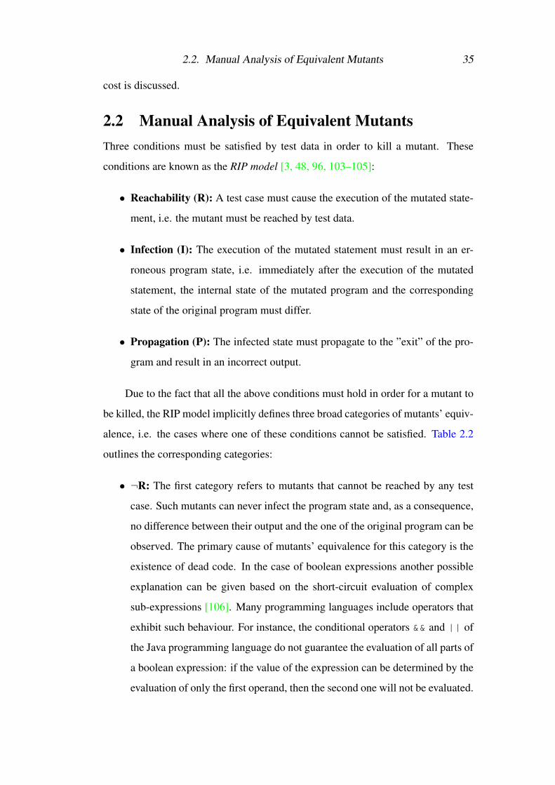
2.2 Manual Analysis of Equivalent MutantsThree conditions must be satisfied by test data in order to kill a mutant. These
conditions are known as the RIP model [3, 48, 96, 103–105]:
• Reachability (R): A test case must cause the execution of the mutated state-
ment, i.e. the mutant must be reached by test data.
• Infection (I): The execution of the mutated statement must result in an er-
roneous program state, i.e. immediately after the execution of the mutated
statement, the internal state of the mutated program and the corresponding
state of the original program must differ.
• Propagation (P): The infected state must propagate to the ”exit” of the pro-
gram and result in an incorrect output.
Due to the fact that all the above conditions must hold in order for a mutant to
be killed, the RIP model implicitly defines three broad categories of mutants’ equiv-
alence, i.e. the cases where one of these conditions cannot be satisfied. Table 2.2
outlines the corresponding categories:
• ¬R: The first category refers to mutants that cannot be reached by any test
case. Such mutants can never infect the program state and, as a consequence,
no difference between their output and the one of the original program can be
observed. The primary cause of mutants’ equivalence for this category is the
existence of dead code. In the case of boolean expressions another possible
explanation can be given based on the short-circuit evaluation of complex
sub-expressions [106]. Many programming languages include operators that
exhibit such behaviour. For instance, the conditional operators && and || of
the Java programming language do not guarantee the evaluation of all parts of
a boolean expression: if the value of the expression can be determined by the
evaluation of only the first operand, then the second one will not be evaluated.

2.3. Cost-Reduction Techniques 36
Table 2.2: Causes of Mutants’ Equivalence (based on the RIP Model).
Category Description
¬R The mutant cannot be reachedR¬I The mutant cannot infect
RI¬P The infected state cannot propagate
Thus, if a mutant affects an operand that will never be evaluated, the mutant
cannot be reached and, thus, can be identified as an equivalent one.
• R¬I: The second category pertains to mutants that can be reached but cannot
infect the original program’s state. The output of such mutants is always the
same as the one of the original program. This situation can be attributed solely
to the change of the mutant or the change of the mutant and the state of the
program at that particular location [106]: for example, if a mutant changes the
statement int i = a to int i = -a and the value of a is always zero
at this program location, then the mutant cannot infect the program state.
• RI¬P: The last category corresponds to mutants that can be reached and can
infect the original program’s state but this infected state cannot propagate to
the ”exit” of the program. Thus, the imposed change can never be discerned.
Two specific cases belong to this particular category [106]: first, the case
where no parts of the infected state can be observed, e.g. an infected variable
that is not used at any return statement; and, second, the case where the
state of the program is infected but, at a later point, this infected state is
coincidentally ”corrected”, e.g. an infected variable that can be returned by
the program but is re-defined before the return statement.
2.3 Cost-Reduction TechniquesAs discussed in the previous sections, mutation is a demanding testing technique. It
requires high computational resources for mutant execution and significant human
effort for equivalent mutant identification.
Researchers have proposed several techniques to manage mutation’s cost. A
2.3. Cost-Reduction Techniques 37
synopsis can be found in the work of Jia and Harman [9] and Madeyski et al. [80].
The former focuses on mutation testing in general, whereas the latter on the equiv-
alent mutant problem in particular. This section describes several of mutation’s
cost-reduction techniques, starting with the ones introduced to tackle the equivalent
mutant problem.
2.3.1 Tackling the Equivalent Mutant Problem
At the core of the equivalent mutant problem is its undecidable nature [89], which
prohibits the creation of fully automated solutions. As a consequence, the prob-
lem is solely amenable to partial, semi-automated ones. Despite this fact, re-
searchers have proposed several techniques to ameliorate its adverse effects. These
approaches can be divided into three general categories2: Equivalent Mutant Re-
duction techniques, Equivalent Mutant Detection techniques and Equivalent Mutant
Classification techniques.
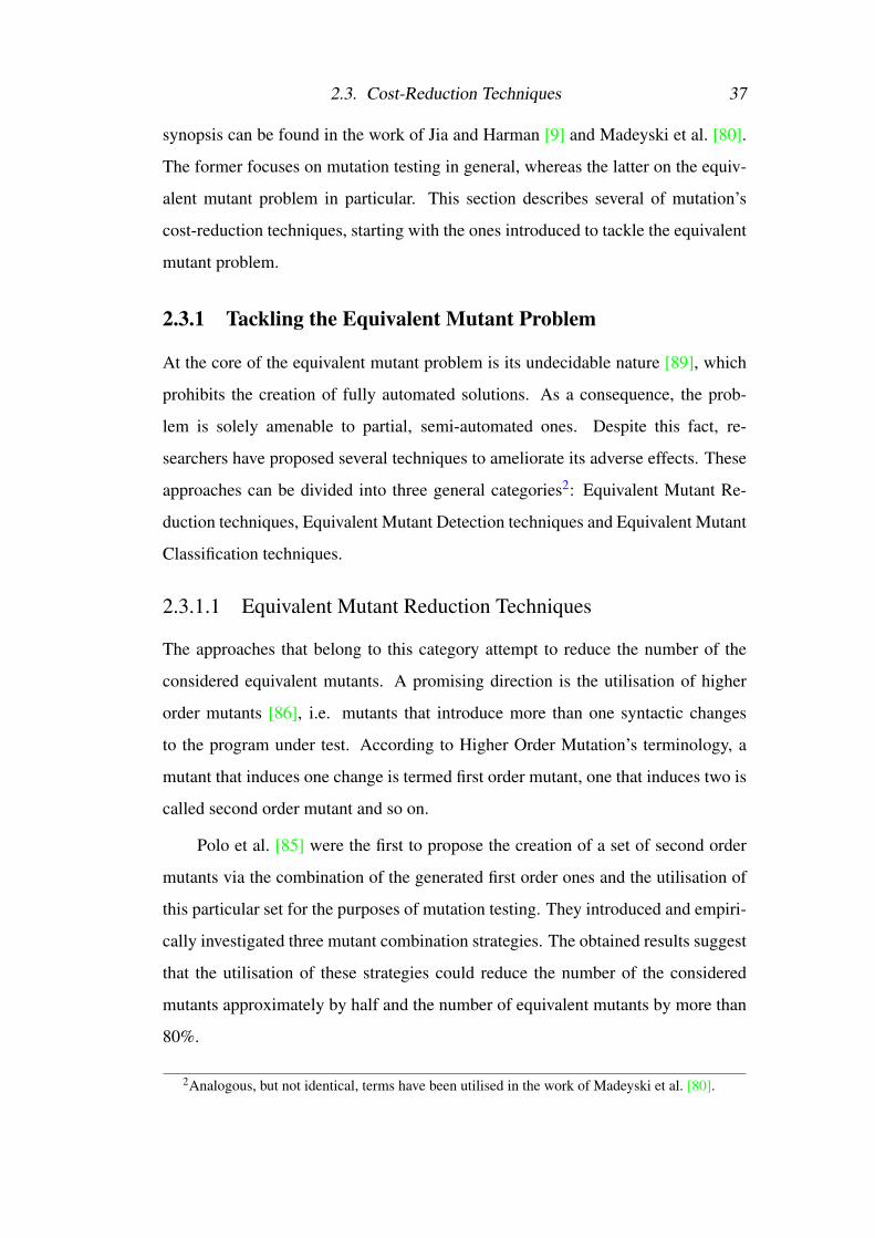
2.3.1.1 Equivalent Mutant Reduction Techniques
The approaches that belong to this category attempt to reduce the number of the
considered equivalent mutants. A promising direction is the utilisation of higher
order mutants [86], i.e. mutants that introduce more than one syntactic changes
to the program under test. According to Higher Order Mutation’s terminology, a
mutant that induces one change is termed first order mutant, one that induces two is
called second order mutant and so on.
Polo et al. [85] were the first to propose the creation of a set of second order
mutants via the combination of the generated first order ones and the utilisation of
this particular set for the purposes of mutation testing. They introduced and empiri-
cally investigated three mutant combination strategies. The obtained results suggest
that the utilisation of these strategies could reduce the number of the considered
mutants approximately by half and the number of equivalent mutants by more than
80%.
2Analogous, but not identical, terms have been utilised in the work of Madeyski et al. [80].
2.3. Cost-Reduction Techniques 38
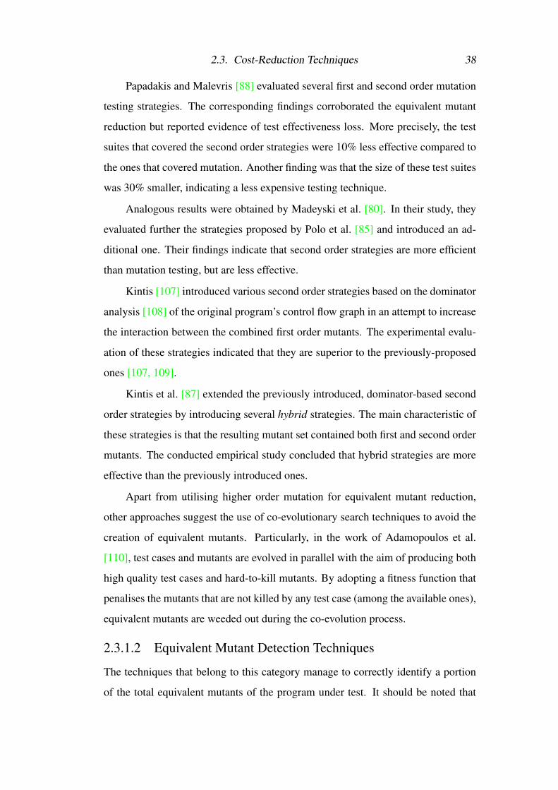
Papadakis and Malevris [88] evaluated several first and second order mutation
testing strategies. The corresponding findings corroborated the equivalent mutant
reduction but reported evidence of test effectiveness loss. More precisely, the test
suites that covered the second order strategies were 10% less effective compared to
the ones that covered mutation. Another finding was that the size of these test suites
was 30% smaller, indicating a less expensive testing technique.
Analogous results were obtained by Madeyski et al. [80]. In their study, they
evaluated further the strategies proposed by Polo et al. [85] and introduced an ad-
ditional one. Their findings indicate that second order strategies are more efficient
than mutation testing, but are less effective.
Kintis [107] introduced various second order strategies based on the dominator
analysis [108] of the original program’s control flow graph in an attempt to increase
the interaction between the combined first order mutants. The experimental evalu-
ation of these strategies indicated that they are superior to the previously-proposed
ones [107, 109].
Kintis et al. [87] extended the previously introduced, dominator-based second
order strategies by introducing several hybrid strategies. The main characteristic of
these strategies is that the resulting mutant set contained both first and second order
mutants. The conducted empirical study concluded that hybrid strategies are more
effective than the previously introduced ones.
Apart from utilising higher order mutation for equivalent mutant reduction,
other approaches suggest the use of co-evolutionary search techniques to avoid the
creation of equivalent mutants. Particularly, in the work of Adamopoulos et al.
[110], test cases and mutants are evolved in parallel with the aim of producing both
high quality test cases and hard-to-kill mutants. By adopting a fitness function that
penalises the mutants that are not killed by any test case (among the available ones),
equivalent mutants are weeded out during the co-evolution process.
2.3.1.2 Equivalent Mutant Detection Techniques
The techniques that belong to this category manage to correctly identify a portion
of the total equivalent mutants of the program under test. It should be noted that

2.3. Cost-Reduction Techniques 39
these techniques reduce mutation’s cost without affecting its effectiveness.
One of the earliest studies is the one of Baldwin and Sayward [111] who sug-
gested the utilisation of compiler optimisation techniques to identify equivalent mu-
tants. The key intuition behind this approach is that mutants are, in a sense, opti-
mised or de-optimised versions of the program under test. In their work, Baldwin
and Sayward proposed six types of compiler optimisation strategies that could iden-
tify equivalent mutants produced by specific mutation operators.
Offutt and Craft [112] implemented the aforementioned strategies in MOTHRA
[91], a mutation testing framework for FORTRAN 77 programs. Their implemen-
tation was based on the data flow analysis of the program under test and utilised
an intermediate representation of this program. The empirical evaluation of these
strategies revealed that they can detect 10% of the equivalent mutants, on average.
The idea of utilising compiler optimisation techniques to identify equivalent
mutants was revisited by Papadakis et al. [113], who investigated whether the avail-
able compiler optimisation strategies of the GCC compiler3 could be leveraged to
identify equivalent mutants. The obtained results suggest that 30% of the equivalent
mutants could be automatically detected, for the studied C programs.
Offutt and Pan [114, 115] proposed another approach to tackle the equiva-
lent mutant problem that is based on mathematical constraints. Specifically, they
formally introduced a heuristic-based set of strategies in order to determine the in-
feasibility of constraint systems that modelled the conditions under which a mutant
can be killed (see also the RIP model in Section 2.2). If such an infeasible con-
straint system is detected, then the corresponding mutant can be safely identified
as equivalent. The experimental evaluation of this approach revealed that it could
detect approximately 50% of the examined equivalent mutants.
Nica and Wotawa [116, 117] proposed a similar technique for equivalent mu-
tant detection. Their approach creates a constraint representation of the program
under test and its mutants and attempts to generate test cases that kill them based
on this representation. If such test cases cannot be generated, then the examined
3https://gcc.gnu.org/

2.3. Cost-Reduction Techniques 40
mutant could be an equivalent one.
Bardin et al. [118] focused on the identification of infeasible test requirements
of several coverage criteria4, including weak mutation (see also Section 2.3.2.4).
The proposed approach combined two static analysis techniques, a forward data
flow analysis (Value Analysis) and a technique to prove program properties (Weak-
est Precondition calculus), to identify weak equivalent mutants, i.e. equivalent mu-
tants generated by the weak mutation technique5. The obtained results suggest that
a considerable number of the weak equivalent mutants generated by the studied
mutation operators can be automatically detected.
Finally, another direction in equivalent mutant identification is the utilisation
of program slicing [122]. Voas and McGraw [123] were the first to propose that
program slicing can identify code locations that are unaffected by some statement
and, thus, should not be mutated because the resulting mutants would be equivalent
ones. Hierons et al. [124] developed this proposal and suggested that amorphous
slicing [125, 126] can be used to support the manual analysis of particularly hard-to-
kill mutants. Finally, Harman et al. [127] showed how dependence-based analysis
can be leveraged to assist in the detection of equivalent mutants.
2.3.1.3 Equivalent Mutant Classification Techniques
Mutant classification has been proposed as another possible direction for equivalent
mutant isolation. The approaches that belong to this category do not detect equiva-
lent mutants, but rather classify mutants as possibly killable or possibly equivalent
ones based on specific characteristics of the program under test. It is postulated that
mutants exhibiting these characteristics are more likely to be killable.
Ellims et al. [128] reported that mutants having the same output as the original
program for a given test suite can have different running profiles in terms of execu-
tion time and CPU and memory usage. Thus, they suggested that such differences
could be used as a means of detecting killable mutants.
4Several studies have also considered ways to circumvent infeasible test requirements, e.g. [119–121].
5Note that if a mutant is equivalent under weak mutation is also equivalent under strong mutation.

2.3. Cost-Reduction Techniques 41
Grun et al. [129] made a similar suggestion: they proposed that changes in
the program behaviour between the original program and one of its mutants could
indicate that the mutant is killable. They investigated whether mutants that impact
the control flow of the original program’s execution are more likely to be killable
ones, and whether the ones that do not are more likely to be equivalent ones. The
obtained results provided evidence supporting this statement.
Schuler et al. [130] examined whether the impact on dynamic invariants is a
good indicator of mutants’ killability. More precisely, their approach deduced pre-
and post-conditions for every function of the program under test from its execution
with test data and examined whether mutants violating such invariants are more
likely to be killable. Its experimental evaluation supported this hypothesis.
Schuler and Zeller [78, 79] investigated further the classification power of the
mutants’ impact on control flow coverage and on methods’ return values. The ob-
tained empirical evidence suggested that impact on coverage is a better indicator of
mutants’ killability than the previously-proposed ones.
Finally, Papadakis and Le Traon [131] and Papadakis et al. [132] investigated
the effectiveness of two mutant classification strategies based on the impact on con-
trol flow coverage. The conducted empirical study revealed that the examined mu-
tant classification strategies managed to reduce the number of the considered equiv-
alent mutants but were less effective than mutation testing.
2.3.2 Reducing Mutation’s Computational Cost
Apart from mutation’s manual effort, mutation requires considerably high compu-
tational resources. As discussed in Section 2.1.3, this computational cost springs
from the fact that a large number of mutants have to be executed, at least once and
potentially many times, against the available test cases. Researchers have proposed
various techniques to deal with this problem. A brief description of several key
approaches follows.

2.3. Cost-Reduction Techniques 42
2.3.2.1 Mutant Sampling
One of the simplest approaches to reduce the number of the considered mutants
is Mutant Sampling [100, 102]. Mutant Sampling selects a small subset of the
generated mutants and performs mutation based on this subset.
Wong [133] investigated different sampling percentages ranging from 10% to
40% in steps of 5%. The experimental results revealed that a sampling percentage of
10% is only 16% less effective than the full set of generated mutants, implying that
mutation testing strategies with a sample percentage greater than 10% form viable
alternatives to mutation. This finding is in accordance to the studies of DeMillo
et al. [91] and King and Offutt [13].
Papadakis and Malevris [88] empirically examined the test effectiveness of
various mutant sampling strategies, ranging from 10% to 60% in steps of 10%.
They found that the recorded test effectiveness loss, ranges between 26% and 6%.
2.3.2.2 Selective Mutation
Selective Mutation [81, 134] is another approximation technique that reduces the
number of the considered mutants. It seeks to find a small set of mutation oper-
ators whose mutants can simulate the mutants generated by all the available op-
erators. Selective Mutation was first introduced by Mathur [135] and was termed
Constrained Mutation.
Mathur [135] proposed the application of mutation without the mutation oper-
ators that generated the most mutants. Offutt et al. [81, 134] developed further this
idea and examined the effectiveness of different, reduced mutation operator sets.
The corresponding findings revealed that from the 22 mutation operators of the
MOTHRA system [91], 5 are sufficient to perform mutation effectively. It should be
mentioned that the number of mutants generated by Selective Mutation is propor-
tional to the number of data references in the program under test (O(Re f s)), which
is considerably smaller than the one of standard mutation (cf. Section 2.1.3).
Barbosa et al. [136] proposed 6 guidelines to determine sufficient mutation op-
erators. The application of these guidelines resulted in a set of 10 operators which
achieved a mutant reduction of 65% with approximately no loss in test effectiveness.
2.3. Cost-Reduction Techniques 43
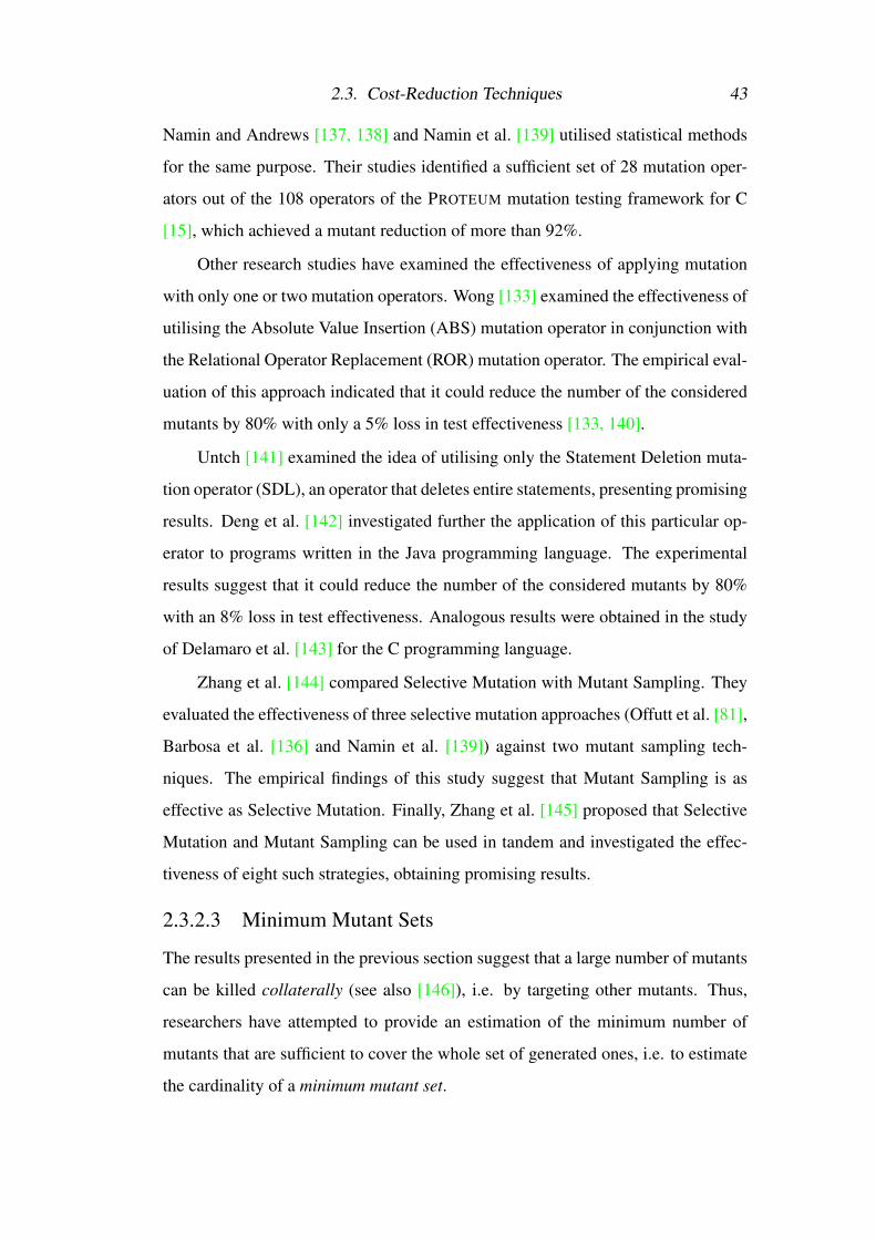
Namin and Andrews [137, 138] and Namin et al. [139] utilised statistical methods
for the same purpose. Their studies identified a sufficient set of 28 mutation oper-
ators out of the 108 operators of the PROTEUM mutation testing framework for C
[15], which achieved a mutant reduction of more than 92%.
Other research studies have examined the effectiveness of applying mutation
with only one or two mutation operators. Wong [133] examined the effectiveness of
utilising the Absolute Value Insertion (ABS) mutation operator in conjunction with
the Relational Operator Replacement (ROR) mutation operator. The empirical eval-
uation of this approach indicated that it could reduce the number of the considered
mutants by 80% with only a 5% loss in test effectiveness [133, 140].
Untch [141] examined the idea of utilising only the Statement Deletion muta-
tion operator (SDL), an operator that deletes entire statements, presenting promising
results. Deng et al. [142] investigated further the application of this particular op-
erator to programs written in the Java programming language. The experimental
results suggest that it could reduce the number of the considered mutants by 80%
with an 8% loss in test effectiveness. Analogous results were obtained in the study
of Delamaro et al. [143] for the C programming language.
Zhang et al. [144] compared Selective Mutation with Mutant Sampling. They
evaluated the effectiveness of three selective mutation approaches (Offutt et al. [81],
Barbosa et al. [136] and Namin et al. [139]) against two mutant sampling tech-
niques. The empirical findings of this study suggest that Mutant Sampling is as
effective as Selective Mutation. Finally, Zhang et al. [145] proposed that Selective
Mutation and Mutant Sampling can be used in tandem and investigated the effec-
tiveness of eight such strategies, obtaining promising results.
2.3.2.3 Minimum Mutant Sets
The results presented in the previous section suggest that a large number of mutants
can be killed collaterally (see also [146]), i.e. by targeting other mutants. Thus,
researchers have attempted to provide an estimation of the minimum number of
mutants that are sufficient to cover the whole set of generated ones, i.e. to estimate
the cardinality of a minimum mutant set.

2.3. Cost-Reduction Techniques 44
Kintis et al. [87] were the first to empirically approximate this number in the
context of the Java programming language. They introduced the concept of disjoint
mutants, that is, mutants whose killing test cases are as disjoint as possible. The
conducted empirical study considered minimal mutant disjointness in the context of
two mutant sets: the set of all generated mutants and the set of hard-to-kill, stub-
born6 ones. The obtained results revealed that only a small portion of the generated
mutants (9%) is required to cover the whole set even in the case of the hard-to-kill
ones (35%).
Ammann et al. [147] investigated further this problem, both theoretically and
empirically. They utilised dynamic subsumption to minimise the number of mu-
tants. Given a test suite, mutant x dynamically subsumes mutant y iff the test cases
that kill x also kill y. The experimental evaluation of dynamic subsumption, in the
context of the C programming language, revealed that only 1.2% of the generated
mutants is required to cover the whole set.
Finally, Kurtz et al. [148, 149] provided additional insights regarding mutant
subsumption and investigated whether dynamic and static analysis techniques can
be used to approximate this relationship. Their findings suggest that static analysis
techniques should be used in tandem with dynamic ones in order to achieve the best
results.
2.3.2.4 Strong, Weak and Firm Mutation
Apart from restricting the number of the considered mutants to manage mutation’s
cost, researchers have introduced various techniques to reduce the execution cost
of running all mutants against the available test suite. The most prominent of these
techniques is Weak Mutation, proposed by Howden [82, 83].
Weak Mutation attempts to reduce the computational resources required to per-
form mutation by avoiding the complete execution of the original program and its
mutants. To achieve this, Weak Mutation redefines the condition that needs to hold
for a mutant to be considered killed (see also the RIP model in Section 2.2): instead
of comparing the final output of the original program and the mutant, the internal
6A stubborn mutant is a killable mutant that is difficult to be killed [106, 124].

2.4. Summary 45
states of these programs are compared immediately after the execution of the mu-
tant or the mutated component. It should be mentioned that standard mutation is
referred to as Strong Mutation when compared with Weak Mutation.
Woodward and Halewood [84] introduced the concept of Firm Mutation, a
mutation approach that occupies the middle ground between Strong and Weak Mu-
tation. They argue that the comparison between the states of the original program
and its mutants can be performed at any point between the first execution of the
mutated statement and the end of the program.
Various research studies corroborate Weak Mutation’s cost-effectiveness. Gir-
gis and Woodward [150] developed a Weak Mutation framework for FORTRAN 77
programs and empirically evaluated its performance. The obtained results suggest
that Weak Mutation requires less computational resources than Strong Mutation.
Horgan and Mathur [151] showed that test suites that satisfy Weak Mutation
can satisfy Strong Mutation with a high probability. Marick [152] presented results
indicating that Weak Mutation is nearly as effective as Strong Mutation. The study
of Kintis et al. [87] revealed that Weak Mutation also reduces mutation’s manual
effort by considering fewer equivalent mutants.
Offutt and Lee [153, 154] evaluated the effectiveness and efficiency of Weak
Mutation, along with different implementations of the technique. Their results sug-
gest that it forms a cost-effective alternative to Strong Mutation. Regarding the
examined implementations, the authors suggest that the internal states of the orig-
inal program and its mutants should be compared after the first execution of the
mutated statement or the basic block that contains it.
2.4 Summary
This chapter presented the core concepts of mutation testing. First, mutation’s fun-
damental hypotheses were described, along with the phases of the traditional mu-
tation analysis process. Next, the cost of mutation per phase was outlined, with
an emphasis on the equivalent mutant problem and its negative effects. Finally,
the conditions that need to hold for a mutant to be equivalent or killable were de-

2.4. Summary 46
tailed and previous work on equivalent mutant elimination, minimum mutant sets
and mutant reduction techniques was introduced.
This chapter presented the necessary background of this thesis. The subsequent
chapters will discuss the techniques that the thesis proposes to tackle the equivalent
mutant problem.

Chapter 3
Equivalent Mutant Isolation via Higher
Order Mutation
As stated in Chapter 2, equivalent mutants constitute a major obstacle to the practi-
cal adoption of mutation. This chapter introduces and empirically evaluates a novel,
mutant classification technique, named Isolating Equivalent Mutants (I-EQM), that
is able to automatically isolate first order equivalent mutants via higher order ones.
In an attempt to ameliorate the adverse effects of the equivalent mutant prob-
lem, Schuler and Zeller [78, 79] suggested a technique, hereafter referred to as the
coverage impact method, that is able to isolate equivalent mutants. This method
is based on the observation that mutants affecting the program execution are more
likely to be killable than those that do not do so [128, 129]. According to this,
mutants can be classified as possibly killable and possibly equivalent ones.
The empirical results of the study of Schuler and Zeller [78, 79] revealed that
75% of the mutants of the resulting possibly killable mutant set were indeed killable
ones. Thus, they suggested that practitioners should target this mutant set in order to
minimise the consequences of equivalent mutants. Although such a practice reduces
the possibility of encountering equivalent mutants, this set was found to include
only the 56% of the total killable ones, thus, missing a large number of them. The
approach described in the present chapter expands the coverage impact method by
aiming at overcoming the aforementioned limitation.
The proposed technique uses second order mutants to isolate possible first or-
der equivalent ones and is the first one to utilise higher order mutants in this context.

48
As mentioned in Chapter 2, a second order mutant is a mutant that induces two syn-
tactic changes to the program under test (see Figure 2.1 for an example).
The approach is based on the intuition that since equivalent mutants have a
small effect on the state of the program, they should not have an apparent impact
on the state of another mutant. Thus, it is argued that a killable mutant is likely to
impact the output of another first order mutant when these mutants are combined,
i.e. forming a second order one. Although such a technique is not clearly competi-
tive to the coverage impact method, it enables the correct classification of different
mutants. This fact motivated the design of a combined classification scheme that
utilises both aforementioned techniques with promising results.
This chapter describes three variations of the proposed technique and investi-
gates their ability to classify killable mutants. Additionally, it empirically validates
the coverage impact method and compares it with the proposed ones. Experimental
evaluation, conducted on two independently selected sets of manually classified mu-
tants, confirms the coverage impact method’s published results and reveals that its
combination with the proposed approaches is capable of retrieving approximately
20% more killable mutants. In general, the contributions of this chapter are the
following:
1. A novel, dynamic method to effectively and automatically classify first order
mutants using second order ones.
2. An empirical study validating the coverage impact method and the proposed
approaches. In particular, the coverage impact method achieves a classifica-
tion precision of 73% and a classification recall of 65%, whereas the proposed
technique realises a precision score of 71% and a recall value of 81%.
3. A manually identified set of killable and equivalent mutants which amplifies
an existing benchmark set [78, 79] and is made publicly available1 with the
aim of enabling replication and comparative studies.
1This set and the results of the present study are publicly available at http://pages.cs.aueb.gr/˜kintism/#stvr2014.

3.1. Background 49
The rest of the chapter is organised as follows. Section 3.1 introduces back-
ground information and briefly describes the coverage impact method. Section 3.2
details the proposed mutant classification schemes and Section 3.3 the conducted
empirical study. Next, Section 3.4 analyses and discusses the obtained results, along
with possible threats to the validity of this study. Finally, Section 3.5 concludes this
chapter, summarising key findings.
3.1 BackgroundThe work presented in this chapter suggests the use of a mutant classification ap-
proach in order to isolate equivalent mutants. The proposed classification scheme
utilises second order mutants and the mutants’ impact in order to highlight the ma-
jority of the killable mutants. This section details these techniques and concepts.
3.1.1 Mutants’ Impact
The approaches studied in this chapter were founded on an assertion, known as the
mutants’ impact, which pertains to killable mutants. The intuition behind mutants’
impact is that mutants altering certain aspects of the original program’s execution
are more likely to be killable. In other words, given a test case, if some aspect
of the execution of the original program and a mutant differs, then the mutant can
be classified as possibly killable. These differences are referred to as the mutants’
impact. Various research studies have investigated how to measure mutants’ impact,
e.g. violated dynamic program invariants [130], different execution program traces
[78, 79, 129] and different methods’ return values [78, 79].
Mutants’ impact represents a variation in the behaviour of the original program
and its mutants. Such differences appear during program executions and, in partic-
ular, after executing the mutated location up to the exit of the program [129]. Along
these lines, impact on coverage measures the differences in the control flow cover-
age between the original program and its mutants [78, 79]. Impact on return values
measures the differences in the values returned by the public methods encountered
during program execution [78, 79]. Impact on dynamic program invariants mea-
sures the number of invariants that were violated by the introduction of mutants

3.1. Background 50
[130].
Generally, it has been empirically found that mutants with impact are more
likely to be killable than those with no impact, regardless of the impact measure
[78, 79]. However, different impact metrics, or their combinations, result in dif-
ferent mutant classifiers with variations in their effectiveness. Constructing a more
effective classifier forms the objective of the present work, which proposes the use
of higher order mutants as impact measures. Based on this novel measure, different
mutants from the previously introduced approaches can be classified appropriately.
3.1.2 Mutation Analysis using Mutant Classifiers
As described in Section 2.1.2, applying mutation testing entails the generation of a
mutant set. Next, the mutants of this set are executed with the available test cases
to determine the killed ones. Finally, the live mutants are analysed by the tester to
produce new test cases or to determine their equivalence. This process iteratively
continues until all killable mutants have been killed.
It can be easily seen that the ratio of the equivalent to killable mutants increases
as more test cases are added to the test suite. This is attributed to the fact that the
number of equivalent mutants remains constant, whereas the number of killable
ones decreases (because they are killed). Thus, if the live mutants could be auto-
matically classified as possibly killable and possibly equivalent ones, considerable
effort savings could be achieved by analysing only the possibly killable mutants
[78, 79, 130, 155].
Based on the aforementioned argument, automated mutant classification ap-
proaches have been proposed in the literature. A typical mutant classification pro-
cess is depicted in Figure 3.1. Steps (a)-(c) divide up the set of live mutants into
two disjoint sets, the possibly killable mutant set and the possibly equivalent one.
Before applying the classification scheme, the set of live mutants must be found,
i.e. the first order mutants of the original program must be generated (Figure 3.1
(a)) and executed with the available test data (Figure 3.1 (b)).
At this point, a set of killed and a set of live mutants have been created. Killed
mutants do not add any value to the testing process and are discarded. In contrast,
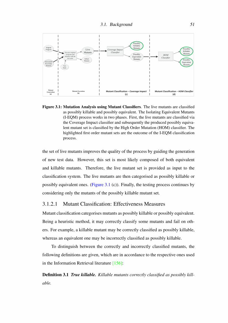
3.1. Background 51
Execute original
program and
mutants with the
test suite
Original
Program Live
Mutants
Killed
Mutants
Test
Suite
Coverage Impact
Classifier
Possibly
Killable
Mutants
Possibly
Equivalent
Mutants
Generated
First Order
Mutants
Mutant
Generation
(a)
Mutant Execution
(b)Mutant Classification – Coverage Impact
(c)
HOM
Classifier
Mutant Classification – HOM Classifier
(d)
Possibly
Killable
Mutants
Possibly
Equivalent
Mutants
Figure 3.1: Mutation Analysis using Mutant Classifiers. The live mutants are classifiedas possibly killable and possibly equivalent. The Isolating Equivalent Mutants(I-EQM) process works in two phases. First, the live mutants are classified viathe Coverage Impact classifier and subsequently the produced possibly equiva-lent mutant set is classified by the High Order Mutation (HOM) classifier. Thehighlighted first order mutant sets are the outcome of the I-EQM classificationprocess.
the set of live mutants improves the quality of the process by guiding the generation
of new test data. However, this set is most likely composed of both equivalent
and killable mutants. Therefore, the live mutant set is provided as input to the
classification system. The live mutants are then categorised as possibly killable or
possibly equivalent ones. (Figure 3.1 (c)). Finally, the testing process continues by
considering only the mutants of the possibly killable mutant set.
3.1.2.1 Mutant Classification: Effectiveness Measures
Mutant classification categorises mutants as possibly killable or possibly equivalent.
Being a heuristic method, it may correctly classify some mutants and fail on oth-
ers. For example, a killable mutant may be correctly classified as possibly killable,
whereas an equivalent one may be incorrectly classified as possibly killable.
To distinguish between the correctly and incorrectly classified mutants, the
following definitions are given, which are in accordance to the respective ones used
in the Information Retrieval literature [156]:
Definition 3.1 True killable. Killable mutants correctly classified as possibly kill-
able.

3.1. Background 52
Definition 3.2 False killable. Equivalent mutants incorrectly classified as possibly
killable.
Definition 3.3 True equivalent. Equivalent mutants correctly classified as possibly
equivalent.
Definition 3.4 False equivalent. Killable mutants incorrectly classified as possibly
equivalent.
To quantify the classification ability and provide a basis for comparison be-
tween the examined approaches, the following measures were utilised. Note that
these metrics are usually employed to compare classifiers in Information Retrieval
experiments [156].
Precision =True killable
True killable+False killable(3.1)
Recall =True killable
True killable+False equivalent(3.2)
Accuracy =True killable+True equivalent
True killable+False killable+True equivalent +False equivalent(3.3)
Fβ = (1+β2)× Precision×Recall
β 2×Precision+Recall(3.4)
Equation 3.1 and Equation 3.2 quantify the ability of the classifier to correctly
classify killable mutants. Specifically, the precision metric quantifies the ability of
the classifier to categorise correctly killable mutants, whereas the recall value mea-
sures the capability of the classifier in retrieving killable mutants. Thus, a high pre-
cision value indicates that the classifier can sufficiently distinguish between killable
and equivalent mutants, whereas a high recall value shows that the classification
scheme is able to recover the majority of the live killable mutants.
Equation 3.3 and Equation 3.4 are utilised to better compare the examined
classifiers. The accuracy metric depicts the percentage of the correctly classified

3.1. Background 53
mutants. The Fβ score2 constitutes a general metric that combines the precision
and recall values into a single measure of overall performance and enables different
weighting between the two measures. Thus, by changing the value of β , different
performance scenarios could be investigated. For instance, a scenario where the
classification precision and recall are equally balanced corresponds to a β value
of 1. In this chapter, three such scenarios are explored, which are described in
Section 3.3.4.
Mutation testing requires the employed test cases to be capable of killing all
killable mutants. Mutant classification changes this requirement to killing all pos-
sibly killable mutants. Thus, mutant classification can be seen as an approximation
method to mutation. The effectiveness of this approximation can be measured as
the number of killable mutants that are correctly classified as such, i.e. by the re-
call metric, because the testing process will be based only on these mutants. The
efficiency of the method can be measured by the number of equivalent mutants that
are incorrectly classified as possibly killable, because these mutants will be manu-
ally analysed by the tester. Thus, the methods’ efficiency can be expressed by the
precision value3 of the classifier.
In general, high precision is difficult to be achieved, but is extremely desirable
for efficiency reasons. However, if high precision is not accompanied by a relatively
high recall, the process might lose some valuable mutants. Because low recall indi-
cates that many killable mutants are ignored, such processes will experience losses
of their strength. On the contrary, high recall is easily achieved by classifying most
or all undetected mutants as possibly killable. In such a case, higher testing quality
is achieved at a considerable cost.
It is obvious that a combination of high precision and high recall is more suit-
able for a mutant classification scheme. In this manner, most of the killable mutants
would be correctly classified as such and, at the same time, testing based on the
retrieved killable mutants can be deemed adequate. In a different situation, the clas-
2For non-negative real values of β .3The percentage of the equivalent mutants that are incorrectly classified as possibly killable is
actually (1− precision). Thus, higher precision indicates that fewer equivalent mutants are to beconsidered and, hence a higher efficiency.

3.2. First Order Mutant Classification via Second Order Mutation 54
sifier would be deficient as it would categorise many equivalent mutants as possibly
killable ones (a case of a classifier with low precision) or it would classify many
killable mutants as possibly equivalent ones (a classifier with low recall). Con-
sequently, it is the reconciliation of a classifier’s precision and recall scores that
stipulates its success.
3.1.2.2 Mutant Classification using Code Coverage
Classifying mutants using code coverage has been empirically found to be superior
to previously proposed classifiers, such as those using dynamic program invariants
and methods’ return values [78, 79]. Following the suggestions of Schuler and
Zeller [78], a coverage measure is determined by counting how many times each
program statement is executed during a test case run. The comparison of the cover-
age measures of both the original program’s and a mutant’s execution results in the
impact measure (coverage difference) of the examined mutant.
Mutants’ impact is defined based on the coverage impact as “the number of
methods that have at least one statement that is executed at a different frequency in
the mutated run than in the normal run, while leaving out the method that contains
the mutated statement” [78]. This approach is also adopted in the present study and
referred to as the Coverage Impact classifier.
3.2 First Order Mutant Classification via Second Or-
der MutationThe primary purpose of this chapter is the introduction of a new mutant classifi-
cation scheme, hereafter referred to as Higher Order Mutation (HOM) classifier,
which would further attenuate the negative effects of the equivalent mutant prob-
lem. The salient feature of the suggested approach is the employment of higher
order mutation in the classification process.
The HOM classifier categorises mutants based on the impact they have on each
other. In view of this, it produces pairs of mutants by combining each examined
(first order) mutant with others. The classifier works based on the intuition that
since equivalent mutants have a small effect on the state of the original program, in

3.2. First Order Mutant Classification via Second Order Mutation 55
a similar fashion, they should also have no apparent impact on the state of another
mutant when combined as a second order mutant. Hence, a possibly equivalent
mutant will have a minor impact on the execution and no observable impact on the
output of another mutant. Any departure from this situation implies that the mutant
is possibly killable, leading to the HOM Classifier Hypothesis.
HOM Classifier’s Hypothesis. Let fom be a first order mutant, umut an un-
classified mutant, umut.fom the second order mutant created by the combination of
the two corresponding mutants and Killable the set of killable mutants of the con-
sidered program under test. The HOM classifier hypothesis states that if the results
of the executions of the first order mutant fom and the second order mutant umut.fom
differ, then the first order mutant umut is killable. More formally:
out putO f ( f om, test) 6= out putO f (umut. f om, test)⇒ umut ∈ Killable
The aforementioned hypothesis forms the basis of the proposed classification
scheme. Thus, if the condition of the aforementioned formula holds, then umut is
classified as possibly killable. Otherwise, umut is classified as possibly equivalent.
This practice is presented in Figure 3.2. Although this condition may not always
hold, the conducted experimental study suggests that it can provide substantial guid-
ance on identifying killable and equivalent mutants.
3.2.1 HOM Classifier: Mutant Classification Process
The mutant classification process of the HOM Classifier requires three main inputs.
These inputs are requisites for the evaluation of the HOM Classifier Hypothesis:
• The first input is the set of the live-unclassified mutants that need to be classi-
fied. The mutants of this set will be categorised as possibly killable or possi-
bly equivalent based on the truth or the falsehood of the classification’s pred-
icate.
• The second required input is the set of mutants, referred to as the classifica-
tion mutant set (CM), that will be used for constructing the sought mutant

3.2. First Order Mutant Classification via Second Order Mutation 56
output
umut
first order mutant
…………………
…………………
…………………
…………………
…………………
…………………
…………………
…………………
…………………
…………………
…………………
umut.fom
second ordermutant
…………………
…………………
…………………
…………………
…………………
…………………
…………………
…………………
…………………
…………………
…………………
fom
first order mutant
…………………
…………………
…………………
…………………
…………………
…………………
…………………
…………………
…………………
…………………
…………………
ProgramUnder Test
…………………
…………………
…………………
…………………
…………………
…………………
…………………
…………………
…………………
…………………
…………………
outputoutput
umut is
killable
output
Test1 Test2 Test3 Test4 Test5 Test6 . . . TestN
Figure 3.2: HOM Classifier’s Hypothesis. The unclassified first order mutant umut isclassified as possibly killable based on its impact on other fom mutants.
pairs. The mutant pairs are constructed by combining these mutants with the
unclassified ones.
• The final input of the classification process is the test suite, with which the
second order mutants and their corresponding first order ones will be exe-
cuted.
Algorithm 3.1 presents the underlying classification process. The algorithm
takes as inputs: (a) the set of the live-unclassified first order mutants; (b) the first
order mutants of the CM set that will be used for the generation of the second order
ones; and, (c) the available test suite. The mutants’ impact is defined as the number
of first order mutants in the CM set whose output is changed after being combined
with the live-unclassified mutant.

3.2. First Order Mutant Classification via Second Order Mutation 57
Algorithm 3.1 HOM Classifier’s Classification Process.Let Live represent the live-unclassified mutant setLet CM represent the classification mutant setLet T represent the available test suiteLet PK represent the resulting set of possibly killable mutantsLet PE represent the resulting set of possibly equivalent mutants
1: PK = /02: PE = /03: foreach umut ∈ Live do4: foreach f om ∈CM do5: foreach test ∈ T do6: fom output = EXECUTEORRETRIEVEOUTPUT(fom, test)7: umut.fom = COMBINE(umut, fom)8: som output = EXECUTEORRETRIEVEOUTPUT(umut.fom, test)9: if fom output 6= som output then
10: PK.ADD(umut)11: continue with the next umut12: end if13: end for14: end for15: PE.ADD(umut)16: end for17: return PK, PE
3.2.1.1 Classification Mutant (CM) Set
As already stated, the proposed classification technique determines the impact of
mutants using other mutants which are referred to as the CM set. For example, in
Figure 3.2, the CM set is the set of the fom mutants to be employed in order to
perform an effective classification process. The question that is raised here is which
mutants are suitable to support the mutant classification process. Specifically, it
has been found that not all mutants are of the same value in assessing the mutants’
impact. Perhaps, by utilising all the available mutants, one could obtain the best
results. However, such an approach is prohibitive because it requires executing all
mutants with all test cases for each mutant to be classified.
Considering the aforementioned issue, a necessary restriction was imposed on
the utilised CM mutant set; only mutants appearing in the same class as the aimed
unclassified mutant were considered. Thus, for each mutant to be classified, a differ-

3.2. First Order Mutant Classification via Second Order Mutation 58
ent CM set was used. This choice was based on the intuition that mutants belonging
to the same class are more likely to interact and be exercised by the same test cases.
It is noted that since there is no available test case able to kill umut, if there is no
interaction between the mutants composing the second order one (umut and fom),
then the outputs of fom and umut.fom will be the same for all the employed test
cases.
3.2.1.2 HOM Classifier Variations
Three variations of the HOM classifier have been considered in the present study:
“HOM classifier (all foms)”, “HOM classifier (killed foms)” and “HOM classifier
(same method foms)”. These approaches differ in the sets of mutants that will be
used for the creation of the second order ones. Recall that the employed CM set
is the one composed of the mutants that belong to the same class as the aimed
unclassified mutant.
The “HOM classifier (all foms)” variation considers the whole CM set,
whereas the other approaches utilise only a specific subset. “HOM classifier (killed
foms)” uses only those mutants that have been killed by the employed test cases,
whereas “HOM classifier (same method foms)” employs only those that appear in
the same method as the aimed unclassified mutant.
The reason for using only the already killed mutants is that these mutants are
more sensitive to the utilised test cases (easy-to-kill) than the live ones and, thus,
they will be more sensitive to the impact of the examined ones. Similarly, using mu-
tants belonging to the same method as the examined mutant increases the chances
of these mutants to be coupled. Besides these reasons, their application was em-
pirically found to be sound. Furthermore, constructing the sought second order
mutants based on the killed mutant set or the mutants of the same method results in
the reduction of the overall computational cost of the technique due to the reduced
number of mutant combinations and their respective executions.
3.2. First Order Mutant Classification via Second Order Mutation 59
3.2.2 Isolating Equivalent Mutants (I-EQM) Classifier
In addition to the techniques described in the previous section, the possibility of em-
ploying a combined strategy is also investigated. To this end, the Isolating Equiva-
lent Mutants (I-EQM) classification scheme is proposed.
The I-EQM classifier constitutes a combination of the coverage impact classi-
fier [78, 79] and the variations of the HOM classifier. The utilisation of the coverage
impact classifier is based on its evaluation, which presented the best results among
those examined in previous studies [78, 79]. Specifically, it resulted in a classifica-
tion precision of 75% and a recall value of 56%.
In addition, the coverage impact classifier manages to successfully classify
most of the mutants that are correctly classified by the rest of the examined ap-
proaches [78, 79]. Due to the fact that the precision measure of the coverage impact
classifier can be considered as an accurate one, i.e. it does not misclassify many
equivalent mutants; effort should be put into improving the recall measure. Achiev-
ing higher recall results in considering a larger number of killable mutants, thus,
strengthening the testing process.
In order to effectively combine different classifiers, they must satisfy the fol-
lowing two requirements: first, the precision of both classification schemes must
be reasonably high; and, second, they should classify different killable mutants as
possibly killable. In other words, both produced sets must be accurate and their
intersection must be of small size. As a result, the precision of the combined classi-
fiers will not be greatly affected, whereas their recall will be significantly improved.
Combining classifiers has been attempted by Schuler and Zeller [78, 79] but without
success.
The I-EQM classification process is summarised in Figure 3.1. After obtain-
ing the set of live mutants (Figure 3.1 (a), (b)), the coverage impact classifier is
employed in order to perform the first step of the I-EQM’s classification procedure
(Figure 3.1 (c)). This step will produce the set of the possibly killable and the
possibly equivalent mutants of the coverage impact classifier.
Next, the HOM classifier is applied to the possibly equivalent mutant set that

3.3. Empirical Study 60
was previously generated (Figure 3.1 (d)). This phase will create the set of the
possibly killable mutants and the set of the possibly equivalent ones of the HOM
classifier. The I-EQM classifier’s resulting set of possibly killable mutants is the
union of the possibly killable mutant set of the coverage impact classifier and the
corresponding killable set of the HOM classifier. The possibly equivalent mutant
set of the I-EQM classifier is the one generated by the HOM classifier. The afore-
mentioned sets appear highlighted in Figure 3.1.
It should be noted that the order in which the coverage impact and HOM clas-
sifiers are applied to the set of live mutants is indifferent, that is, the resulting sets
of the possibly killable and the possibly equivalent mutants would be the same re-
gardless of the application order of the two classifiers. This is due to the fact that
the resulting set of the possibly killable mutants will be composed of the mutants
that are categorised as such by at least one of the combined classifiers. The possibly
equivalent mutant set will contain the mutants that are categorised as such by all the
combined classifiers. This can also be generalised to a classification process that
includes more than two classifiers.
3.3 Empirical StudyThe present study investigates a new aspect of higher order mutants, their ability to
classify first order ones. This characteristic constitutes the basis of the HOM and
I-EQM classifiers, detailed in the previous section.
The present section describes the empirical evaluation of these approaches,
which is based on two independently selected sets of manually classified mutants
and directly compares them to the coverage impact classifier [78, 79]. Additionally,
a revalidation of the coverage impact classifier is performed.
3.3.1 Research Questions
The following research points summarise the primary purpose of the presented em-
pirical evaluation:
• RQ 3.1 Can second order mutation provide adequate guidance in equivalent
mutant isolation, or equally, how effective are the HOM and I-EQM classi-

3.3. Empirical Study 61
Table 3.1: Subject Program Details.
Program Description Version LOC Test CasesAspectJ AOP extension to Java cvs: 2007-09-15 25,913 336Barbecue Bar code creator svn: 2007-11-26 4,837 153Commons Helper utilities svn: 2009-08-24 19,583 1,608Jaxen XPath engine svn: 2008-12-03 12,438 689Joda-Time Date and time library svn: 2009-08-17 25,909 3,497JTopas Parser tools 1.0 (SIR) 2,031 128XStream XML object serialisation svn: 2009-09-02 16,791 1,122
fiers in terms of their recall and precision metrics?
• RQ 3.2 Do the HOM and I-EQM classifiers perform better than the coverage
impact classifier?
• RQ 3.3 How stable is the categorisation ability of the HOM, I-EQM and
coverage impact classifiers across the two different mutant sets? Are there
any important differences between the two sets?
3.3.2 Subject Programs and Supporting Tool
The evaluation of the examined classification schemes is based on a set of seven
open source projects. The motivation behind the selection of these test subjects is
twofold. First, they were also used in the empirical evaluation of the coverage im-
pact classifier [78, 79], hence they facilitate a direct comparison. Second, these pro-
grams constitute real-world examples and therefore would provide valuable insights
into the practical applicability and the efficacy of the examined mutant classification
techniques.
Table 3.1 presents the corresponding details. Specifically, the table reports the
subjects’ name, a brief description of their usage, their versions, the lines of code
and the number of accompanying test cases. It should be noted that in the case of
AspectJ, only the org.aspectj.ajdt.core package was considered.
For mutant generation and execution, the JAVALANCHE mutation testing
framework (version 0.3.6) [20] for the Java programming language was utilised.

3.3. Empirical Study 62
Table 3.2: JAVALANCHE’s Mutation Operators.
Mutation Operator Description
Replace Numerical Constant (RNC)Replaces a numerical constant instanceby +1, −1 or 0
Negate Jump Condition (NJC)Inserts the negation operator to logicalconditional instances
Replace Arithmetic Operator (RAO)Replaces an arithmetic operator instanceby another one
Omit Method Calls (OMC)Omits a method call and replaces it witha default value (the default value replacesthe returned one)
The main reason for selecting this framework is because it implements the cov-
erage impact classification method and it was utilised in its empirical evalua-
tion. JAVALANCHE enables the efficient application of mutation by implement-
ing a large number of optimisations and has been used in many previous studies
[78, 79, 129, 130, 157], providing evidence of its usefulness. Table 3.2 records
details about the mutation operators supported by the tool.
3.3.3 Benchmark Mutant Sets
In order to investigate the effectiveness of the proposed approaches, the mutant
set of the studies of Schuler and Zeller [78, 79] was utilised, hereafter referred to
as “control mutant set 1”. “Control mutant set 1” is composed of 140 manually
classified mutants, each one belonging to a different class of the subject programs,
with a total number of 20 mutants per test subject.
To avoid overfitting or coincidental results, a second set of mutants was also
considered. The second set, referred to as “control mutant set 2”, was constructed
for the purposes of the present study, in a similar fashion to “control mutant set
1”. Specifically, for each test subject, 10 live mutants were randomly selected for
manual classification, each one belonging to a different class. Thus, “control mutant
set 2” is comprised of 70 manually classified mutants, with a total number of 10
mutants per test subject.
Details about the considered control mutant sets with respect to the examined
programs and utilised mutation operators are recorded in Table 3.3 and Table 3.4.

3.3. Empirical Study 63
Table 3.3: Control Mutant Sets’ Profile w.r.t. Subject Programs.
Considered Mutants Manually Classified MutantsSubject Number of Reached Killable EquivalentProgram Mutants Mutants Set1 Set2 Sets1+2 Set1 Set2 Sets1+2
AspectJ 6,613 2,878 15 6 21 5 4 9Barbecue 3,283 1,603 14 9 23 6 1 7Commons 8,693 8,305 6 6 12 14 4 18Jaxen 6,619 3,944 10 7 17 10 3 13Joda-Time 5,322 4,197 14 7 21 6 3 9JTopas 1,676 1,402 10 4 14 10 6 16XStream 2,156 1,730 8 5 13 12 5 17Total 34,362 24,059 77 44 121 63 26 89
The former presents the number of killable and equivalent mutants per control mu-
tant set and subject program and the latter, the same information per mutation oper-
ator. manually identified set. It must be noted that these sets are among the largest
manually analysed sets of mutants utilised in the literature (cf. Table 4 in the study
of Yao et al. [106]).
More precisely, the “Considered Mutants” column of Table 3.3 refers to the
number of the considered mutants, among those generated by the JAVALANCHE
framework. It should be mentioned that the considered mutants are the ones that be-
long to the same classes as the manually classified ones. Column “Number of Mu-
tants” presents the total number of the corresponding mutants and column “Reached
Mutants”, the ones reached by the available test cases. Finally, the “Manually Clas-
sified Mutants” column reports the number of the equivalent and killable mutants
among the manually classified ones.
Table 3.4 records the contribution of each mutation operator to the employed
control mutant sets. Specifically, the number of mutants per operator and the num-
ber of killable and equivalent ones are reported. From the table, it can be ob-
served that the Replace Numerical Constant (RNC) and Replace Arithmetic Op-
erator (RAO) operators contribute 20% more equivalent mutants than the Negate
Jump Condition (NJC) and Omit Method Calls (OMC) operators.
By examining the two control mutant sets, it can be seen that they have dif-
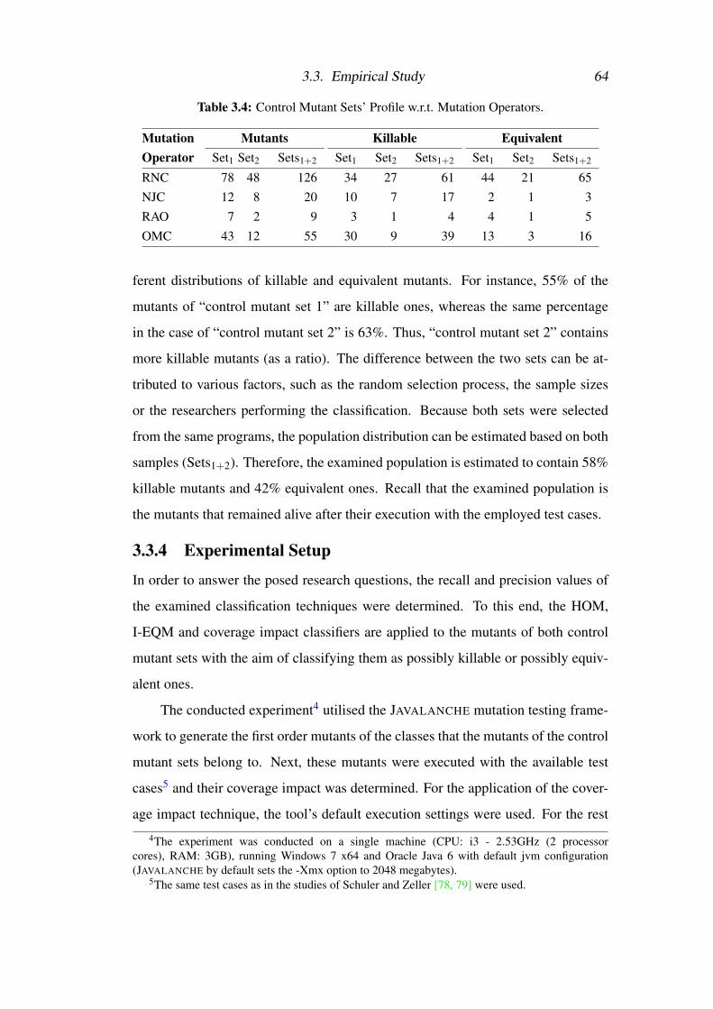
3.3. Empirical Study 64
Table 3.4: Control Mutant Sets’ Profile w.r.t. Mutation Operators.
Mutation Mutants Killable EquivalentOperator Set1 Set2 Sets1+2 Set1 Set2 Sets1+2 Set1 Set2 Sets1+2
RNC 78 48 126 34 27 61 44 21 65NJC 12 8 20 10 7 17 2 1 3RAO 7 2 9 3 1 4 4 1 5OMC 43 12 55 30 9 39 13 3 16
ferent distributions of killable and equivalent mutants. For instance, 55% of the
mutants of “control mutant set 1” are killable ones, whereas the same percentage
in the case of “control mutant set 2” is 63%. Thus, “control mutant set 2” contains
more killable mutants (as a ratio). The difference between the two sets can be at-
tributed to various factors, such as the random selection process, the sample sizes
or the researchers performing the classification. Because both sets were selected
from the same programs, the population distribution can be estimated based on both
samples (Sets1+2). Therefore, the examined population is estimated to contain 58%
killable mutants and 42% equivalent ones. Recall that the examined population is
the mutants that remained alive after their execution with the employed test cases.
3.3.4 Experimental Setup
In order to answer the posed research questions, the recall and precision values of
the examined classification techniques were determined. To this end, the HOM,
I-EQM and coverage impact classifiers are applied to the mutants of both control
mutant sets with the aim of classifying them as possibly killable or possibly equiv-
alent ones.
The conducted experiment4 utilised the JAVALANCHE mutation testing frame-
work to generate the first order mutants of the classes that the mutants of the control
mutant sets belong to. Next, these mutants were executed with the available test
cases5 and their coverage impact was determined. For the application of the cover-
age impact technique, the tool’s default execution settings were used. For the rest
4The experiment was conducted on a single machine (CPU: i3 - 2.53GHz (2 processorcores), RAM: 3GB), running Windows 7 x64 and Oracle Java 6 with default jvm configuration(JAVALANCHE by default sets the -Xmx option to 2048 megabytes).
5The same test cases as in the studies of Schuler and Zeller [78, 79] were used.
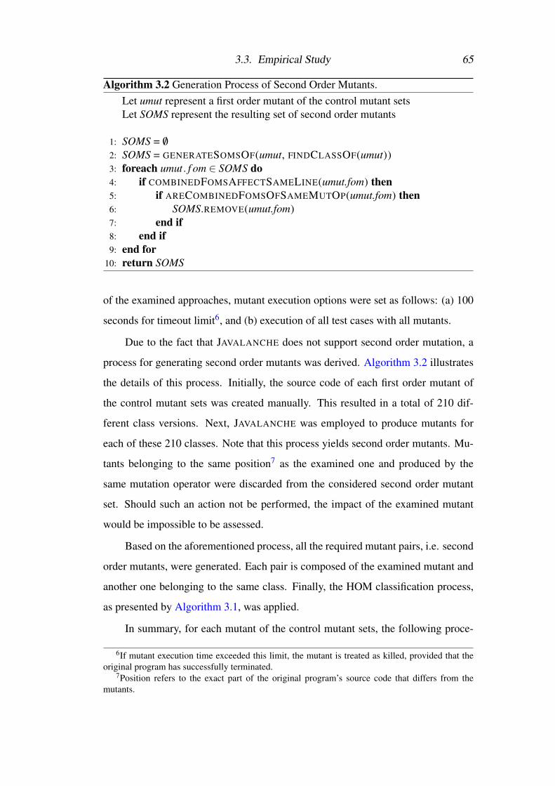
3.3. Empirical Study 65
Algorithm 3.2 Generation Process of Second Order Mutants.Let umut represent a first order mutant of the control mutant setsLet SOMS represent the resulting set of second order mutants
1: SOMS = /02: SOMS = GENERATESOMSOF(umut, FINDCLASSOF(umut))3: foreach umut. f om ∈ SOMS do4: if COMBINEDFOMSAFFECTSAMELINE(umut.fom) then5: if ARECOMBINEDFOMSOFSAMEMUTOP(umut.fom) then6: SOMS.REMOVE(umut.fom)7: end if8: end if9: end for
10: return SOMS
of the examined approaches, mutant execution options were set as follows: (a) 100
seconds for timeout limit6, and (b) execution of all test cases with all mutants.
Due to the fact that JAVALANCHE does not support second order mutation, a
process for generating second order mutants was derived. Algorithm 3.2 illustrates
the details of this process. Initially, the source code of each first order mutant of
the control mutant sets was created manually. This resulted in a total of 210 dif-
ferent class versions. Next, JAVALANCHE was employed to produce mutants for
each of these 210 classes. Note that this process yields second order mutants. Mu-
tants belonging to the same position7 as the examined one and produced by the
same mutation operator were discarded from the considered second order mutant
set. Should such an action not be performed, the impact of the examined mutant
would be impossible to be assessed.
Based on the aforementioned process, all the required mutant pairs, i.e. second
order mutants, were generated. Each pair is composed of the examined mutant and
another one belonging to the same class. Finally, the HOM classification process,
as presented by Algorithm 3.1, was applied.
In summary, for each mutant of the control mutant sets, the following proce-
6If mutant execution time exceeded this limit, the mutant is treated as killed, provided that theoriginal program has successfully terminated.
7Position refers to the exact part of the original program’s source code that differs from themutants.
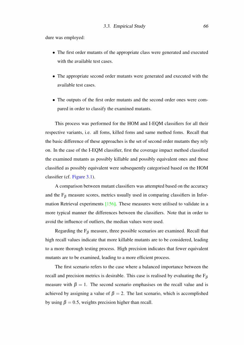
3.3. Empirical Study 66
dure was employed:
• The first order mutants of the appropriate class were generated and executed
with the available test cases.
• The appropriate second order mutants were generated and executed with the
available test cases.
• The outputs of the first order mutants and the second order ones were com-
pared in order to classify the examined mutants.
This process was performed for the HOM and I-EQM classifiers for all their
respective variants, i.e. all foms, killed foms and same method foms. Recall that
the basic difference of these approaches is the set of second order mutants they rely
on. In the case of the I-EQM classifier, first the coverage impact method classified
the examined mutants as possibly killable and possibly equivalent ones and those
classified as possibly equivalent were subsequently categorised based on the HOM
classifier (cf. Figure 3.1).
A comparison between mutant classifiers was attempted based on the accuracy
and the Fβ measure scores, metrics usually used in comparing classifiers in Infor-
mation Retrieval experiments [156]. These measures were utilised to validate in a
more typical manner the differences between the classifiers. Note that in order to
avoid the influence of outliers, the median values were used.
Regarding the Fβ measure, three possible scenarios are examined. Recall that
high recall values indicate that more killable mutants are to be considered, leading
to a more thorough testing process. High precision indicates that fewer equivalent
mutants are to be examined, leading to a more efficient process.
The first scenario refers to the case where a balanced importance between the
recall and precision metrics is desirable. This case is realised by evaluating the Fβ
measure with β = 1. The second scenario emphasises on the recall value and is
achieved by assigning a value of β = 2. The last scenario, which is accomplished
by using β = 0.5, weights precision higher than recall.

3.4. Empirical Findings 67
In the present experiment, special care was taken to handle certain cases be-
cause of some inconsistencies of the utilised tool. Specifically, it was observed that
in the case of execution timeouts, the tool gave different results when some mutants
were executed in isolation than together with others. To circumvent this problem,
in the case of the HOM and I-EQM classifiers, when mutants were categorised as
possibly killable owing to timeout conditions (if either the first order mutant or the
second order one resulted in a timeout), the corresponding mutants of the considered
mutant pairs were isolated and re-executed individually with an increased timeout
limit.
Similarly, in the case of the coverage impact, the mutants that were classified
differently with respect to the previous study [78], were re-executed in isolation with
a greater timeout limit. Although the previous study’s results [78] could be used,
this would constitute a potential threat to the validity of the comparison because of
the different execution environments and the use of “control mutant set 2”.
Other special considerations include issues concerning the comparison of the
programs’ output. Note that such a comparison is performed between every first
order mutant and its respective second order one. Many programs had outputs de-
pendent on each specific execution. Execution outputs containing time informa-
tion, e.g. the Joda-Time and AspectJ test subjects, or directory locations, e.g.
JTopas, are examples of such cases. To effectively handle these situations, the ex-
ecution dependent portions of the considered outputs were replaced with predefined
values via the employment of appropriate regular expressions.
3.4 Empirical Findings
3.4.1 RQ 3.1 and RQ 3.2: Precision and Recall
The evaluation results of the coverage impact classifier are recorded in Table 3.5,
which presents the classification precision and recall for the examined control mu-
tant sets and test subjects. On average, the coverage impact method achieves a
precision of 72% and a recall of 66% for “control mutant set 1”. In the case of
“control mutant set 2”, the obtained precision score is 76% and the corresponding

3.4. Empirical Findings 68
Table 3.5: Mutant Classification using the Coverage Impact Classifier.
Subject ProgramPossibly Killable Set 1 Possibly Killable Set 2Precision Recall Precision Recall
AspectJ 72% 87% 60% 100%Barbecue 77% 71% 100% 89%Commons 0% 0% 100% 17%Jaxen 57% 40% 100% 43%Joda-Time 79% 79% 57% 57%JTopas 100% 80% 100% 50%XStream 56% 63% 67% 80%Total 72% 66% 76% 64%
Table 3.6: Mutant Classification using the HOM Classifier: Control Mutant Set 1 (w.r.t. allfoms, killed foms and same method foms variations).
Subject ProgramPossibly killable Set 1
Precision RecallAll Killed Method All Killed Method
AspectJ 73% 73% 80% 53% 53% 27%Barbecue 90% 88% 88% 64% 50% 50%Commons 50% 50% 67% 67% 67% 67%Jaxen 67% 63% 60% 60% 60% 30%Joda-Time 82% 90% 90% 64% 64% 64%JTopas 100% 100% 100% 30% 30% 30%XStream 42% 45% 42% 63% 63% 63%Total 69% 70% 71% 57% 55% 45%
recall value is 64%.
It is noted that these results were obtained by executing JAVALANCHE with
the settings described in the previous section. Thus, the difference between the
aforementioned results and the ones reported in the respective studies of Schuler
and Zeller [78, 79] is attributed to the execution environment used for performing
the present study.
The respective results of the HOM classifier are recorded in Table 3.6 and Ta-
ble 3.7, for the corresponding control mutant sets. Both tables have similar structure
to Table 3.5, except that each figure of each cell refers to a different variation of the
method. Thus, the first figure corresponds to the “HOM classifier (all foms)” varia-
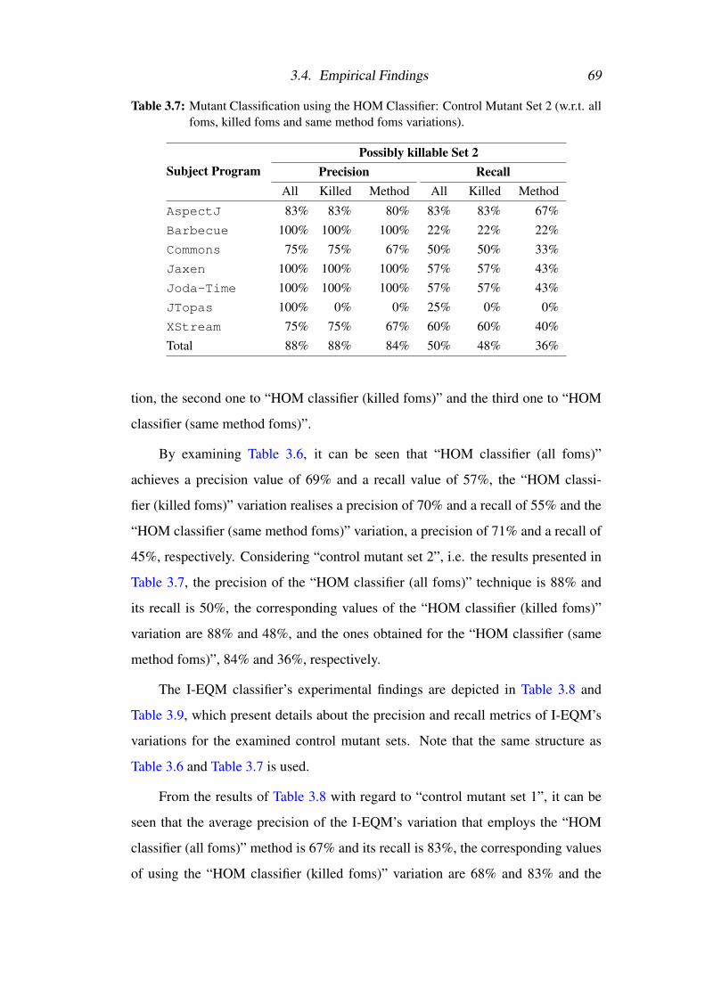
3.4. Empirical Findings 69
Table 3.7: Mutant Classification using the HOM Classifier: Control Mutant Set 2 (w.r.t. allfoms, killed foms and same method foms variations).
Subject ProgramPossibly killable Set 2
Precision RecallAll Killed Method All Killed Method
AspectJ 83% 83% 80% 83% 83% 67%Barbecue 100% 100% 100% 22% 22% 22%Commons 75% 75% 67% 50% 50% 33%Jaxen 100% 100% 100% 57% 57% 43%Joda-Time 100% 100% 100% 57% 57% 43%JTopas 100% 0% 0% 25% 0% 0%XStream 75% 75% 67% 60% 60% 40%Total 88% 88% 84% 50% 48% 36%
tion, the second one to “HOM classifier (killed foms)” and the third one to “HOM
classifier (same method foms)”.
By examining Table 3.6, it can be seen that “HOM classifier (all foms)”
achieves a precision value of 69% and a recall value of 57%, the “HOM classi-
fier (killed foms)” variation realises a precision of 70% and a recall of 55% and the
“HOM classifier (same method foms)” variation, a precision of 71% and a recall of
45%, respectively. Considering “control mutant set 2”, i.e. the results presented in
Table 3.7, the precision of the “HOM classifier (all foms)” technique is 88% and
its recall is 50%, the corresponding values of the “HOM classifier (killed foms)”
variation are 88% and 48%, and the ones obtained for the “HOM classifier (same
method foms)”, 84% and 36%, respectively.
The I-EQM classifier’s experimental findings are depicted in Table 3.8 and
Table 3.9, which present details about the precision and recall metrics of I-EQM’s
variations for the examined control mutant sets. Note that the same structure as
Table 3.6 and Table 3.7 is used.
From the results of Table 3.8 with regard to “control mutant set 1”, it can be
seen that the average precision of the I-EQM’s variation that employs the “HOM
classifier (all foms)” method is 67% and its recall is 83%, the corresponding values
of using the “HOM classifier (killed foms)” variation are 68% and 83% and the

3.4. Empirical Findings 70
Table 3.8: Mutant Classification using the I-EQM Classifier: Control Mutant Set 1. (w.r.t.all foms, killed foms and same method foms variations).
Subject ProgramPossibly killable Set 1
Precision RecallAll Killed Method All Killed Method
AspectJ 74% 74% 72% 93% 93% 87%Barbecue 75% 75% 75% 86% 86% 86%Commons 40% 40% 50% 67% 67% 67%Jaxen 60% 60% 63% 60% 60% 50%Joda-Time 76% 81% 81% 93% 93% 93%JTopas 100% 100% 100% 90% 90% 90%XStream 40% 43% 40% 75% 75% 75%Total 67% 68% 69% 83% 83% 81%
Table 3.9: Mutant Classification using the I-EQM Classifier: Control Mutant Set 2. (w.r.t.all foms, killed foms and same method foms variations).
Subject ProgramPossibly killable Set 2
Precision RecallAll Killed Method All Killed Method
AspectJ 60% 60% 60% 100% 100% 100%Barbecue 100% 100% 100% 89% 89% 89%Commons 75% 75% 67% 50% 50% 33%Jaxen 100% 100% 100% 71% 71% 71%Joda-Time 63% 63% 63% 71% 71% 71%JTopas 100% 100% 100% 75% 50% 50%XStream 63% 63% 63% 100% 100% 100%Total 76% 76% 75% 80% 77% 75%
ones obtained by utilising “HOM classifier (same method foms)” are 69% and 81%,
respectively8.
With respect to “control mutant set 2”, i.e. the results of Table 3.9, the I-EQM
classifier’s variation that utilises the “HOM classifier (all foms)” technique realises
a precision score of 76% and a recall value of 80%, the one that employs the “HOM
classifier (killed foms)” variation achieves a precision of 76% and a recall of 77%,
whereas the variation that uses “HOM classifier (same method foms)” achieves a
8The difference between these results and the previously published ones [155] is due to thecoverage impact method’s re-evaluation; the previous results were based on the reported results ofSchuler and Zeller [78], whereas the new ones on the method’s re-evaluation

3.4. Empirical Findings 71
precision and recall value of 75%.
These results provide evidence that the HOM Classifier Hypothesis is an ap-
propriate mutant classification property. Therefore, the employment of second order
mutation can be beneficial to equivalent mutant isolation. Additionally, the results
of the HOM classifier’s variations indicate that the utilisation of only the killed, first
order mutants as the CM set achieves approximately the same classification effec-
tiveness as the employment of all the generated first order mutants. Regarding the
“HOM classifier (same method foms)” technique, it is less effective than the other
two variations, but in most cases is more efficient because of the reduced size of the
considered CM set.
By considering the above-mentioned facts, the utilisation of the “HOM clas-
sifier (killed foms)” technique is advised, mainly because it is more efficient than
“HOM classifier (all foms)”. Compared with the coverage impact classifier, the
HOM classifier attains lower precision and recall values, indicating that the cover-
age impact classifier is a better one.
Regarding the I-EQM classifier’s results, it is evident that it forms an effective
classification scheme. It achieves to retrieve more than 80% of the killable mutants
with a reasonably high precision of approximately 70% for each control mutant set.
This high retrieval capability is attributed to the ability of the HOM classifier to
classify different killable mutants than the coverage impact one. As a consequence,
their combination enhances the corresponding recall value by nearly 20%, meaning
that approximately 20% more killable mutants are to be considered.
To better compare these two classifiers, Table 3.10 presents the classification
precision and recall values of the coverage impact technique when applied to the
union of the control mutant sets and Table 3.11 the same results for I-EQM’s vari-
ations. Note that the tables are structured in a similar manner to the previously
described ones.
On average, the coverage impact method achieves a classification precision of
73% and a recall value of 65%. The I-EQM classifier’s variation that uses the “HOM
classifier (all foms)” approach realises a precision score of 70% and a recall value of

3.4. Empirical Findings 72
Table 3.10: Mutant Classification using the Coverage Impact Classifier: Control MutantSets 1+2.
Subject ProgramPossibly Killable Sets 1+2Precision Recall
AspectJ 68% 90%Barbecue 86% 78%Commons 33% 8%Jaxen 70% 41%Joda-Time 71% 71%JTopas 100% 71%XStream 60% 69%Total 73% 65%
Table 3.11: Mutant Classification using the I-EQM Classifier: Control Mutant Sets 1+2.(w.r.t. all foms, killed foms and same method foms variations).
Subject ProgramPossibly killable Sets 1+2
Precision RecallAll Killed Method All Killed Method
AspectJ 69% 69% 68% 95% 95% 90%Barbecue 83% 83% 83% 87% 87% 87%Commons 50% 50% 55% 58% 58% 50%Jaxen 73% 73% 77% 65% 65% 59%Joda-Time 72% 75% 75% 86% 86% 86%JTopas 100% 100% 100% 86% 79% 79%XStream 48% 50% 48% 85% 85% 85%Total 70% 71% 71% 82% 81% 79%
82%, the one that employs the “HOM classifier (killed foms)” variation achieves a
precision of 71% and a recall of 81%, and the variation that utilises “HOM classifier
(same method foms)” achieves a precision of 71% and a recall value of 79%.
These results indicate that the coverage impact technique, by realising a recall
score of 65%, misses 35% of the killable mutants, thus, leading to a potential in-
effective testing process. In contrast, all three variations of I-EQM realise a high
recall value, with a maximum recall of 82%, thus, improving the effectiveness of
the testing process by considering 17% more killable mutants and by achieving a
reasonably high precision score.
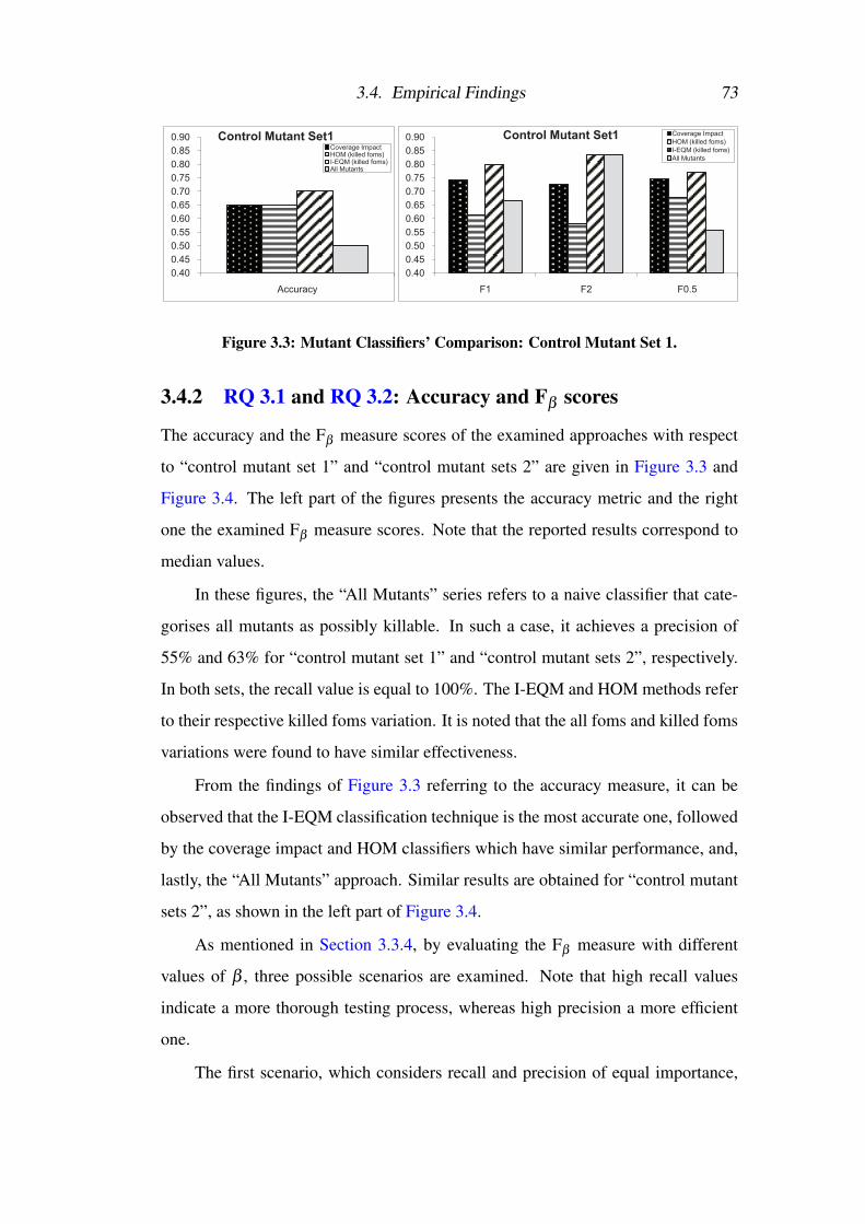
3.4. Empirical Findings 73
0.40
0.45
0.50
0.55
0.60
0.65
0.70
0.75
0.80
0.85
0.90
Accuracy
Control Mutant Set1Coverage ImpactHOM (killed foms)I-EQM (killed foms)All Mutants
0.40
0.45
0.50
0.55
0.60
0.65
0.70
0.75
0.80
0.85
0.90
F1 F2 F0.5
Control Mutant Set1 Coverage Impact
HOM (killed foms)
I-EQM (killed foms)
All Mutants
Accuracy
Coverage ImpactHOM (killed foms)
EQM (killed foms)All Mutants
F1 F2 F0.5
Coverage Impact
HOM (killed foms)
EQM (killed foms)
All Mutants
Accuracy
Coverage Impact
HOM (killed foms)
EQM (killed foms)
All Mutants
F1 F2 F0.5
Coverage ImpactHOM (killed foms)
EQM (killed foms)All Mutants
Figure 3.3: Mutant Classifiers’ Comparison: Control Mutant Set 1.
3.4.2 RQ 3.1 and RQ 3.2: Accuracy and Fβ scores
The accuracy and the Fβ measure scores of the examined approaches with respect
to “control mutant set 1” and “control mutant sets 2” are given in Figure 3.3 and
Figure 3.4. The left part of the figures presents the accuracy metric and the right
one the examined Fβ measure scores. Note that the reported results correspond to
median values.
In these figures, the “All Mutants” series refers to a naive classifier that cate-
gorises all mutants as possibly killable. In such a case, it achieves a precision of
55% and 63% for “control mutant set 1” and “control mutant sets 2”, respectively.
In both sets, the recall value is equal to 100%. The I-EQM and HOM methods refer
to their respective killed foms variation. It is noted that the all foms and killed foms
variations were found to have similar effectiveness.
From the findings of Figure 3.3 referring to the accuracy measure, it can be
observed that the I-EQM classification technique is the most accurate one, followed
by the coverage impact and HOM classifiers which have similar performance, and,
lastly, the “All Mutants” approach. Similar results are obtained for “control mutant
sets 2”, as shown in the left part of Figure 3.4.
As mentioned in Section 3.3.4, by evaluating the Fβ measure with different
values of β , three possible scenarios are examined. Note that high recall values
indicate a more thorough testing process, whereas high precision a more efficient
one.
The first scenario, which considers recall and precision of equal importance,

3.4. Empirical Findings 74
0.40
0.45
0.50
0.55
0.60
0.65
0.70
0.75
0.80
0.85
0.90
Accuracy
Control Mutant Set2
Coverage ImpactHOM (killed foms)I-EQM (killed foms)All Mutants
0.40
0.45
0.50
0.55
0.60
0.65
0.70
0.75
0.80
0.85
0.90
F1 F2 F0.5
Control Mutant Set2 Coverage Impact
HOM (killed foms)
I-EQM (killed foms)
All Mutants
Accuracy
Coverage Impact
HOM (killed foms)
EQM (killed foms)
All Mutants
F1 F2 F0.5
Coverage ImpactHOM (killed foms)
EQM (killed foms)All Mutants
Figure 3.4: Mutant Classifiers’ Comparison: Control Mutant Set 2.
is represented by the F1 measure (β = 1). The corresponding results, depicted
in the right part of Figure 3.3 and Figure 3.4, suggest that the I-EQM approach
outperforms the rest.
The second scenario, described by the F2 measure (β = 2), emphasises on
the recall value. It can be seen that the I-EQM classification approach achieves
far better results than the coverage impact and HOM techniques for both examined
control mutant sets, but worse than the “All Mutants” classifier for “control mutant
set 2”. This is expected, because the “All Mutants” categorises all examined mutants
as possibly killable.
The last scenario, which limits the selection of equivalent mutants, favours the
precision metric over the recall one. For this case, described by the F0.5 measure
(β = 0.5), the I-EQM classifier achieves better results than the rest of the examined
approaches for “control mutant set 1”. Regarding “control mutant set 2”, the I-EQM
classifier achieves approximately the same (slightly worse) results as the coverage
impact one. However, in this case, the HOM classifier scores better than the rest.
Generally, the I-EQM classification method provides better results than the
coverage impact one with respect to accuracy and all the considered scenarios. De-
spite the variation of HOM classifier’s classification ability between the two control
mutant sets, I-EQM achieves a higher accuracy for both examined sets. This fact
indicates that the coverage impact and HOM classifiers detect-classify different mu-
tants, hence their combination is effective.
Figure 3.5 presents the overall, i.e. with respect to the union of the control mu-

3.4. Empirical Findings 75
0.40
0.45
0.50
0.55
0.60
0.65
0.70
0.75
0.80
0.85
0.90
Accuracy
Control Mutant Sets 1 + 2
Coverage Impact
HOM (killed foms)
I-EQM (killed foms)
All Mutants
0.40
0.45
0.50
0.55
0.60
0.65
0.70
0.75
0.80
0.85
0.90
F1 F2 F0.5
Control Mutant Sets 1 + 2 Coverage ImpactHOM (killed foms)I-EQM (killed foms)All Mutants
Figure 3.5: Mutant Classifiers’ Comparison: Control Mutant Sets 1+2.
tant sets, accuracy and Fβ measure scores of the classification approaches. Again,
the results refer to the killed foms variations of the I-EQM and HOM classifiers
using median values. From the presented findings, it can be argued that I-EQM
constitutes a better mutant classifier than the rest of the examined approaches.
3.4.3 RQ 3.3: Classifiers’ Stability
In order to examine the stability of the considered classifiers across the test subjects,
the standard deviation of the precision and recall metrics with respect to the union of
the control mutant sets was calculated per examined technique. Figure 3.6 displays
these findings. The columns of the charts depict the mean precision and recall
values per utilised program for each of the examined approaches, and, the vertical
bars, the corresponding values that lie within one standard deviation of the mean.
Again, the presented results for the HOM and I-EQM techniques refer to the killed
foms variation.
Regarding precision, the coverage impact technique presents the greatest varia-
tion among the examined methods with a standard deviation of 21%. The HOM and
I-EQM classifiers demonstrate similar variation levels of approximately 18%. With
respect to the recall metric, the coverage impact approach experiences a variation
level of 28%, whereas the HOM and I-EQM classifiers 16% and 13%, respectively.
From the presented data, it can be concluded that the I-EQM approach tends to
be more stable than the rest of the examined techniques. To visualise the variation
among the precision and recall values of the classifiers, Figure 3.7 presents two
groups of boxplots for the corresponding measures. It can be seen that the coverage

3.4. Empirical Findings 76
0.00
0.20
0.40
0.60
0.80
1.00
Precision
Coverage Impact HOM I-EQM
0.00
0.20
0.40
0.60
0.80
1.00
Recall
Coverage Impact HOM I-EQM
Figure 3.6: Classifiers’ Stability. Mean and standard deviation of the precision and recallmetrics for control mutant sets 1+2.
impact (CI) and I-EQM techniques have a similar spread regarding their precision
values, with coverage impact having a slight advantage. However, regarding the
recall values, the I-EQM is clearly better.
By comparing the three classification approaches based on the results presented
both here and in the previous subsections, it becomes evident that the I-EQM tech-
nique manages to provide better recall values with only a minor loss on its precision
and with the highest level of stability, for the examined test subjects.
3.4.4 Statistical Analysis
In order to investigate whether the previously described differences among the ex-
amined classifiers are statistically significant, the Wilcoxon Signed Rank Test was
employed per compared technique. The Wilcoxon Signed Rank Test is a non-
parametric test for two paired samples that tests whether or not the two populations
from which the corresponding samples are drawn are identical. A non-parametric
test was utilised, instead of a parametric one, because it is based on no distributional
assumptions for the considered data observations.
A series of two-tailed hypothesis tests were performed to investigate whether
the HOM and I-EQM classifiers have similar effectiveness to the coverage impact
technique, regarding the precision and recall metrics. For example, the hypotheses
that were tested in the case of the HOM classifier, regarding its precision metric, are
the following:

3.4. Empirical Findings 77
0.00
0.20
0.40
0.60
0.80
1.00
CI HOM I-EQM
(a) Precision
0.00
0.20
0.40
0.60
0.80
1.00
CI HOM I-EQM
(b) Recall
Figure 3.7: Variation of the Classifiers’ Precision and Recall Metrics: Control MutantSets 1+2.
H0: The HOM and Coverage Impact classifiers perform the same with regard to
the precision metric.
H1: The HOM and Coverage Impact classifiers perform differently with regard to
the precision metric.
Similar hypotheses were tested with respect to the I-EQM classifier and the
recall metric. A significance level of α = 0.05 was employed for all conducted tests.
Thus, the tests reject the null hypothesis H0 if a p-value smaller than α is obtained;
otherwise the null hypothesis is accepted. Table 3.12 presents the corresponding
findings.
The first column of the table refers to the considered effectiveness measures,
the second one to the classification methods being compared and the last one
presents the obtained p-values (two-tailed). Regarding the precision metric, the
null hypothesis is rejected only in the case of “HOM versus I-EQM”, i.e. there is a
statistically significant difference in the effectiveness of the two classifiers. For the
remaining cases, i.e. “CI versus HOM” and “CI versus I-EQM”, the null hypothesis

3.4. Empirical Findings 78
Table 3.12: Statistical Significance based on the Wilcoxon Signed Rank Test.
Compared Techniquesp-value
(two-tailed)
PrecisionCI versus HOM 0.094CI versus I-EQM 0.563HOM versus I-EQM 0.031
RecallCI versus HOM 0.469CI versus I-EQM 0.016HOM versus I-EQM 0.031
is accepted.
With respect to the recall measure, the null hypothesis is rejected in the cases
of “CI versus I-EQM” and “HOM versus I-EQM”, thus, it can be concluded that
there is strong evidence to establish a difference in the effectiveness of the I-EQM
classifier with respect to the HOM and coverage impact methods. Finally, in the
case of “CI versus HOM”, the null hypothesis is accepted.
These findings suggest that there is statistically insufficient evidence to estab-
lish a difference in the performance of the coverage impact and I-EQM classifiers,
concerning precision. On the contrary, there is a strong, statistically significant dif-
ference in their performance regarding recall, with a p-value of 0.016.
3.4.5 Discussion
Comparing the coverage impact method’s results between the two sets, a slight
increase in the precision metric for “control mutant set 2” and a minor decrease in
the corresponding recall value can be observed. These variations indicate that the
coverage impact’s classification ability is not greatly affected by different mutants.
Considering the classification results of the HOM classifier, the aforemen-
tioned trend is also present, i.e. the precision for “control mutant set 2” is increased
while its recall is decreased. It must be mentioned that in this case, the deviation
is higher, indicating that HOM’s classification ability is more affected by different
mutants than the one of the coverage impact technique.
Finally, the trend observed for the previous classifiers is consistent with the
differences between the results of the I-EQM technique. Concerning its results, it is

3.4. Empirical Findings 79
obvious that I-EQM manages to enhance the recall of the coverage impact technique
for both examined control mutant sets (Table 3.8 and Table 3.9) while maintaining
its precision at a reasonably high level.
Another aspect of the presented results that should be noted relates to the
“HOM classifier (same method foms)” approach. By examining the entries of Ta-
ble 3.6 and Table 3.7, it is apparent that this approach experiences a decrease of
nearly 10% on its recall value compared with the other variations of the HOM clas-
sifier (i.e., killed foms and all foms) and approximately 20% compared with the
one of the coverage impact method. Interestingly, the I-EQM (same method foms)
classification scheme, according to Table 3.11, suffers only a loss of 3% compared
with the rest of the approaches of the I-EQM classifier and has an enhanced recall
of nearly 15% compared with the coverage impact classifier. These findings sug-
gest that the majority of the misclassified killable mutants of the coverage impact
classifier can be correctly classified by the “HOM classifier (same method foms)”
variation.
Generally, the application of the I-EQM classifier on the studied subjects re-
sults in the identification of 81% of the live killable mutants and 46% of the total
equivalent mutant instances. The coverage impact classifier identifies 65% of the
live killable mutants and 33% of the equivalent ones. These values suggest that
by killing the identified killable mutants, a mutation score9 such as 95.2% will be
achieved for the coverage impact technique and one of 97.4% for I-EQM. There-
fore, it becomes obvious that a more thorough testing process is established by the
I-EQM method. However, this is borne with the overhead of analysing 1.17% more
equivalent mutants10.
3.4.6 Mutants with Higher Impact
The behaviour of the considered approaches with respect to higher impact values is
also investigated. To this end, the impact values of the examined mutants based on
9These scores were evaluated by counting the mutants killed by the employed tests plus theidentified killable mutants of the totally estimated killable ones.
10This number was evaluated by counting the identified equivalent mutants of the totally estimatednumber of equivalent ones.

3.4. Empirical Findings 80
the coverage impact and HOM classifiers are determined for both examined control
mutant sets.
Note that the impact value of a mutant based on the coverage impact technique
is defined as “the number of methods that have at least one statement that is executed
at a different frequency in the mutated run than in the normal run, while leaving out
the method that contains the mutated statement” [78]. The corresponding impact
value of the HOM classifier is defined as the number of first order mutants in the
CM set whose output has changed after being combined with the live-unclassified
mutant (see also Section 3.2.)
Figure 3.8 presents the results of the coverage impact technique for both ex-
amined control mutant sets. The left part of the figure provides information about
the precision metric (y-axis) and how it changes according to different impact value
thresholds (x-axis). Based on different thresholds, different mutants are classified
as possibly killable or possibly equivalent. For instance, by employing a thresh-
old value of 50, mutants with higher impact values will be classified as possibly
killable, otherwise they will be classified as possibly equivalent.
From the left part of the figure, it can be seen that for impact values lower
than 20, the precision metric increases, whereas for impact values between 20 and
100, the opposite holds. Note that the highest precision scores are obtained when
the impact value thresholds are between 10 and 20. The right part of the figure
describes a plot between precision (y-axis) and the percentage of mutants with the
highest impact (x-axis); for example, an x1 value of 0.2 indicates that 20% of these
mutants are examined. Thus, lower values of the x-axis represent mutants with
higher impact values.
It can be observed that, in general, the precision metric decreases as the per-
centage of the examined mutants with the highest impact decreases. Consider the
top 10% of the mutants with the highest impact (i.e. x1 = 0.1), by examining only
these mutants a precision value of approximately 70% is obtained. In contrast, by
examining the top 30%, a precision score of 80% is realised. These findings suggest
that an analogy between mutants with the highest impact and high killability ratios

3.4. Empirical Findings 81
0
0.2
0.4
0.6
0.8
1
0 10 20 30 40 50 60 70 80 90 100
Pre
cisi
on
Impact threshold
Precision w.r.t. impact values
0
0.2
0.4
0.6
0.8
1
0 0.1 0.2 0.3 0.4 0.5 0.6 0.7 0.8 0.9 1
Pre
cisi
on
Mutants with highest impact
Precision w.r.t. mutants with the highest impact
Set1
Set2
Figure 3.8: Coverage Impact Classifier: Higher Impact Values. The left part of thefigure presents the precision metric w.r.t. impact values and the right one, pre-cision w.r.t. mutants with the highest impact.
0
0.2
0.4
0.6
0.8
1
0 10 20
Pre
cisi
on
Impact threshold
Precision w.r.t. impact values
0
0.2
0.4
0.6
0.8
1
0 0.1 0.2 0.3 0.4 0.5 0.6 0.7 0.8 0.9 1
Pre
cisi
on
Mutants with highest impact
Precision w.r.t. mutants with the highest impact
Set1
Figure 3.9: HOM Classifier: Higher Impact Values. The left part of the figure presentsthe precision metric w.r.t. impact values and the right one, precision w.r.t. mu-tants with the highest impact.
cannot be drawn.
Figure 3.9 depicts the same results as Figure 3.8 in the case of the HOM clas-
sifier. By examining the two figures, it is apparent that the same trends exist.
In conclusion, it can be argued that mutants with the highest impact do not nec-
essarily guarantee the highest killability ratios. On the contrary, the results suggest
that the precision metric for higher impact values decreases. This trend is in accor-
dance with the findings of Schuler and Zeller [78, 79], where the precision of the top
25% of the mutants with the highest impact was found higher than the one obtained
by examining only the top 15% (cf. Table IX [78]). The presented results indicate
that the relationship between impact and killability needs further investigation.
To investigate the differences between “control mutant set 1” and “control mu-
tant set 2”, Figure 3.10 illustrates the coverage impact’s classification precision (y-

3.4. Empirical Findings 82
0
0.1
0.2
0.3
0.4
0.5
0.6
0.7
0.8
0.9
1
0 2 4 6 8 10 12
Pre
cisi
on
Impact threshold
Set1 vs Set2
Set1
Set2
Figure 3.10: Differences between Studied Control Mutant Sets. Coverage Impact Clas-sifier’s precision w.r.t. impact values for “control mutant set 1” and “controlmutant set 2”.
axis) with respect to the different impact value thresholds (x-axis). It must be noted
that the maximum impact value considered for this diagram is 12 because it is the
maximum impact value of “control mutant set 2”.
From this graph, it can be observed that for impact values lower than 8, both
sets demonstrate a similar behaviour. For impact values greater than 8, the precision
of “control mutant set 1” remains approximately the same, whereas the one of “con-
trol mutant set 2” decreases. Overall, due to the fact that the differences between
the two sets are small, it is believed that the above-mentioned conclusions hold for
both studied sets.
3.4.7 Threats to Validity
This section discusses potential threats to the validity of the present study. Threats
to the internal, external and construct validity are presented, along with the actions
taken to mitigate their consequences.
• Internal Validity. The internal validity concerns the degree of confidence in
the causal relationship of the studied factors and the observed results. One
such factor is the utilisation of the specified test subjects and the use of the
JAVALANCHE framework. As mentioned in Section 3.3.2, their choice was
mainly based on enabling a direct comparison between the proposed clas-

3.4. Empirical Findings 83
sification techniques and the coverage impact classifier. Owing to the fact
that the employed subjects are large in size and of different application do-
mains, they are considered as appropriate. Furthermore, various empirical
studies, e.g. [78, 79, 130, 157], utilised the same tool, thus, increasing the
confidence in its results. The employed mutation operators constitute an-
other possible issue. Different operator sets, as those suggested by Offutt
et al. [81], might give different classification results. However, the present
study focuses on mutants’ impact, which is believed to be an attribute inde-
pendent of the nature of the studied mutants [79]. Additionally, the present
study replicates the findings of the coverage impact technique [78, 79], thus
it is natural to use the same mutants. Another potential threat that falls into
this category concerns the employed test suites. It is possible that different
test suites could produce different classification results. However, the utilised
test suites were independently created by the developers of the considered
programs without using mutation testing. Furthermore, the manually classi-
fied mutants were randomly selected among those that were executed and not
killed by the employed test cases. These two facts give confidence in that the
studied methods can provide useful guidance in increasing the quality of the
testing process and that the mutants’ impact constitutes an effective mutant
classification property that can lead to a better testing process.
• External Validity. The external validity of an experiment refers to the poten-
tial threats that inhibit the generalisation of its results. The generalisation of
a study’s results is difficult to be achieved because of the range of different
aspects that the experimental study must consider. The results presented in
this chapter are no exception. Despite this, actions have been taken to atten-
uate the effects of these threats. First, the empirical evaluation of this study
was based on a benchmark set of real-world programs which has been used
in similar research studies, e.g. [78, 79, 130, 157]. Second, the examined
programs vary in size and complexity. Finally, the evaluation of the proposed
classification techniques was based on two independently created sets of man-

3.5. Summary 84
ually classified mutants; one created for the evaluation of the coverage impact
classifier [78, 79] and the other, for the purposes of the present experimental
study.
• Construct Validity. The construct validity refers to the means of defining the
employed measurement of an experiment and the extent to which it measures
the intended properties. A possible threat pertains to the manual classification
of the mutants of the examined control mutant sets. The mutants classified as
killable pose no threat as the basis of their classification is a test case that
is able to “kill” them, whereas the mutants classified as equivalent could do
so due to the complexity of the involved manual analysis. To ameliorate the
effects of this threat, the studied programs and control mutant sets were made
publicly available.
3.5 SummaryThis chapter introduced a novel mutant classification technique, named Higher Or-
der Mutation (HOM) classifier. The originality of the proposed technique stems
from the fact that it leverages higher order mutation to automatically isolate first
order equivalent mutants. Specifically, the HOM classifier utilises second order
mutation to classify a given set of first order mutants as possibly killable or possi-
bly equivalent ones.
This chapter also investigated the possibility of introducing a combined mutant
classification scheme. To this end, the Isolating Equivalent Mutants (I-EQM) clas-
sifier was proposed. I-EQM combines the HOM classifier with the state-of-the-art
Coverage Impact classifier.
The conducted empirical study, based on two independently developed sets
of manually analysed mutants, revealed that I-EQM managed to correctly classify
more killable mutants than the other studied approaches with approximately no loss
on its precision, indicating that I-EQM is a better mutant classifier. This finding was
also supported by the performed statistical analysis.
Additionally, the relationship between mutant’ impact and killability was in-

3.5. Summary 85
vestigated. The obtained results indicate that mutants with the highest impact do
not necessarily guarantee the highest killability ratios. On the contrary, for higher
impact values the precision metric decreased. These results suggest that the rela-
tionship between impact and killability warrants further investigation.
The introduced mutant classification technique, albeit more powerful than the
previously proposed ones, cannot overcome the inherent characteristics of mutant
classification, i.e. the possibility of misclassifying mutants. The next chapter intro-
duces and formally describes a series of data flow patterns that can be leveraged to
automatically identify equivalent mutants.

Chapter 4
Equivalent Mutant Detection via Data Flow
Patterns
Detecting equivalent mutants is an arduous task, primarily due to the undecidable
nature of the underlying problem. Chapter 3 introduced a mutant classification
technique that managed to automatically isolate possibly equivalent mutants, thus,
ameliorating their adverse effects. This chapter also targets the equivalent mutant
problem by focusing on specific source code locations that can generate equivalent
mutants.
Harman et al. [127] proposed the use of dependence analysis [158] as a means
of avoiding the generation of equivalent mutants. This chapter augments their work
by formalising a set of data flow patterns that can reveal source code locations able
to generate equivalent mutants. For each pattern, a formal definition is given, based
on the Static Single Assignment (SSA) [159, 160] intermediate representation of the
program under test, and the necessary conditions implying the pattern’s existence
in the program’s source code are described. By identifying such problematic sit-
uations, the introduced patterns can provide advice on code locations that should
not be mutated and can automatically detect equivalent mutants that belong to these
locations.
Apart from dealing with equivalent mutants, the proposed patterns are able to
identify specific paths for which a mutant is functionally equivalent to the origi-
nal program; such a mutant is termed partially equivalent. Thus, if one of these
paths is to be executed with test data, the output of the mutant and the original pro-
4.1. Background 87
gram would be the same. This knowledge can be leveraged by test case generation
techniques in order to avoid targeting these paths when attempting to kill partially
equivalent mutants.
The contributions of this chapter can be summarised in the following points:
1. The introduction and formal definition of nine problematic data flow patterns
that are able to automatically detect equivalent and partially equivalent mu-
tants.
2. An empirical study, based on a set of approximately 800 manually identified
mutants from several open source projects, which indicates that the intro-
duced patterns exist in real-world software and provides evidence regarding
their detection power.
It should be mentioned that Chapter 5 examines further the proposed data flow
patterns. More precisely, it introduces an automated framework, named Mutants’
Equivalence Discovery (MEDIC), which implements the corresponding patterns
and empirically assesses the tools’ effectiveness and efficiency.
The rest of the chapter is organised as follows: Section 4.1 introduces the
necessary background information and Section 4.2 details the proposed data flow
patterns along with illustrative examples. In Section 4.3, the empirical study and
the obtained results are presented. Finally, Section 4.4 summarises this chapter.
4.1 Background
4.1.1 Employed Mutation Operators
As mentioned in Section 2.1, mutation’s effectiveness depends largely on the em-
ployed set of mutation operators. The present study considers the mutation opera-
tors utilised by the MUJAVA mutation testing framework [19]. MUJAVA is a mutation
testing tool for the Java programming language that has been widely used in the lit-
erature of mutation testing. Note that the utilisation of this particular set does not
reduce the applicability of the proposed data flow patterns since analogous mutation
operators have been developed for other programming languages and have been in-

4.1. Background 88
Table 4.1: Mutation operators of MUJAVA.
Mutation Operator DescriptionArithmetic Operator Replacement {(op1,op2) | op1,op2 ∈ {+,-,*,/,%} ∧Binary (AORB) op1 6= op2}Arithmetic Operator Replacement {(op1,op2) | op1,op2 ∈ {++,--} ∧Short-Cut (AORS) op1 6= op2}Arithmetic Operator Insertion {(v,-v)}Unary (AOIU)
Arithmetic Operator Insertion {(v,--v),(v,v--),(v,++v),(v,v++)}Short-cut (AOIS)
Arithmetic Operator Deletion {(+v,v),(-v,v)}Unary (AODU)
Arithmetic Operator Deletion {(--v,v),(v--,v),(++v,v),(v++,v)}Short-cut (AODS)
Relational Operator Replacement {((a op b), false),((a op b), true),(ROR) (op1, op2) | op1,op2 ∈ {>,>=,<,<=,
==,!=}∧op1 6= op2}Conditional Operator Replacement {(op1,op2) | op1,op2 ∈ {&&,||,∧ } ∧(COR) op1 6= op2}Conditional Operator Deletion {(!cond,cond)}(COD)
Conditional Operator Insertion {(cond, !cond)}(COI)
Shift Operator Replacement {(op1,op2) | op1,op2 ∈ {>>,>>>,(SOR) <<} ∧ op1 6= op2}Logical Operator Replacement {(op1,op2) | op1,op2 ∈ {&,|,∧ } ∧(LOR) op1 6= op2}Logical Operator Insertion {(v,∼v)}(LOI)
Logical Operator Deletion {(∼v,v)}(LOD)
Short-Cut Assignment Operator {(op1,op2) | op1,op2 ∈ {+=,-=,*=,Replacement (ASRS) /=, %=,&=,|=,∧=,>>=,>>>=,
<<=}∧ op1 6= op2}
corporated into appropriate tools, e.g. the Unary Operator Insertion (UOI) of the
MILU mutation testing tool [16] for C.

4.1. Background 89
MUJAVA is based on the selective mutation approach, i.e. it utilises a sub-
set of mutation operators that are considered particularly effective (see also Sec-
tion 2.3.2.2). Table 4.1 presents the employed mutation operators, along with a
brief description of the imposed changes. In total, the tool implements 15 muta-
tion operators, which fall into 6 general categories: arithmetic operators, relational
operators, conditional operators, shift operators, logical operators, and assignment
operators.
The Arithmetic Operator Insertion Short-cut (AOIS) mutation operator inserts
the pre- and post-increment and decrement arithmetic operators to valid variables
of the original program. The inserted post-increment or decrement operators are
of particular interest. The basic characteristic of such operators is that they do not
change the value of the affected variable at the evaluation of the affected expres-
sion. The variable is used unchanged and the next time it is referenced, it will be
incremented or decremented by one. As discussed in Section 4.2.2, the application
of these operators can result in the generation of equivalent mutants.
Note that the AOIS operator is not specific to Java: other programming lan-
guages, e.g. C, support such arithmetic operators and other mutation tools have im-
plemented it as well, e.g. the PROTEUM mutation testing tool [15] for C. The data
flow patterns of the Use-Def and Use-Ret categories, described in Section 4.2.2,
detect problematic situations where the application of this operator results in the
creation of equivalent mutants.
4.1.2 Static Single Assignment (SSA) Form
The definition of the proposed data flow patterns is based on an intermediate repre-
sentation of the program under test, which is known as the Static Single Assignment
(SSA) form [159, 160]. Many modern compilers use the SSA form to represent
internally the input program and perform various optimisations. Furthermore, sev-
eral research studies have utilised the SSA form as a means of program analysis,
e.g. [161].
The basic characteristic of the SSA representation is that each variable of the
program under test is assigned exactly once. More precisely, for each assignment

4.2. Equivalent Mutants and Data Flow Analysis 90
v = 4x = v + 5v = 6y = v + 7
(a) Source Code Fragment.
v1 = 4x1 = v1 + 5v2 = 6y1 = v2 + 7
(b) Its SSA representation.
Figure 4.1: Static Single Assignment Form Example. (adapted from [162]).
to a variable, that variable is given a unique name and all its uses reached by that
assignment are appropriately renamed [162]. Figure 4.1 depicts an example of a
code fragment and its SSA form (adapted from the work of Cytron et al. [162]): the
left part of the figure illustrates the source code fragment and the right one, its SSA
representation.
Cytron et al. [162] presented the first algorithm to efficiently translate a pro-
gram to its SSA form. Note that this translation restricts the definition points of
a variable: after the translation, each variable is bound to have only one defini-
tion point, instead of multiple in the original program (cf. variables v1, v2 and v
of Figure 4.1). This fact enables a more compact representation of the underly-
ing data flow information and facilitates powerful code analysis and optimisation
techniques. This simple example suffices for the purposes of this chapter, a more
detailed one is presented in Section 5.1 of Chapter 5.
4.2 Equivalent Mutants and Data Flow AnalysisThis work focuses on detecting equivalent mutants by leveraging the data flow in-
formation of the program under test. To this end, the SSA representation of the
program is utilised. This is believed to lead to a more powerful analysis and a
clearer definition of the conditions that need to hold for a particular situation to be
pathogenic.
Four groups of problematic patterns are introduced: the Use-Def (UD), the
Use-Ret (UR), the Def-Def (DD) and the Def-Ret (DR) categories of patterns. The
first two categories target equivalent mutants that are due to mutation operators that
insert the post-increment (e.g. var++) or decrement (e.g. var−−) arithmetic
operators or other similar operators. The remaining categories target problematic

4.2. Equivalent Mutants and Data Flow Analysis 91
situations that are caused by mutation operators that affect variable definitions, e.g.
the Arithmetic Operator Replacement Binary (AORB) mutation operator.
The search for these patterns is performed on the source code of the original
program. Therefore, these patterns can be used in two ways: (a) they can be in-
corporated into mutation testing frameworks to avoid the generation of equivalent
mutants, or (b) in the case where the mutants have already been generated, they
can be used to detect equivalent or partially equivalent mutants. Before elaborating
on these categories, the necessary functions, used in the patterns’ definitions, are
described.
4.2.1 Function Definitions
This subsection introduces a set of functions that will be used in the definition of
the problematic data flow cases. First, functions related to the control and data flow
of the program under test are described and, subsequently, the concept of a partially
equivalent mutant is formally introduced.
4.2.1.1 Control Flow Functions
reach(p,s, t) Denotes that path p traverses nodes s and t, starting at node s and
ending at node t. Note that s and t need not be the starting and
ending nodes of the corresponding control flow graph.
f rstIns(i) A function that returns the first instruction of the node that con-
tains instruction i.
bb(i) A function that returns the node which contains instruction i.
isExit(n) Denotes that node n contains a statement that forces the program
to exit.
The aforementioned functions utilise the control flow analysis of the program
under test. Note that the terms node and basic block are used interchangeably;
the nodes of a Control Flow Graph (CFG) are the basic blocks of the respective
program. For the purposes of this study: a path is a sequence of two or more nodes,
where each pair of adjacent nodes represents an edge of the corresponding CFG and

4.2. Equivalent Mutants and Data Flow Analysis 92
an instruction is considered to be a simple statement that belongs to a single line
and one basic block.
4.2.1.2 Data Flow Functions
de f (vx) A function that returns the instruction that defines variable vx.
use(n,vx) A function that returns the instruction that contains the nth use of
variable vx.
de f A f tr(i,vx) A function that returns the instruction of the first definition of the
variable of the original program denoted by vx, after instruction
i. The scope of this function is limited to the basic block that
contains instruction i.
useB f r(i,vx) A function that returns the instruction of the first use of the vari-
able of the original program denoted by vx, before instruction i.
The scope of this function is limited to the basic block that con-
tains instruction i.
useA f r(i,vx) A function that returns the instruction of the first use of the vari-
able of the original program denoted by vx, after instruction i. The
scope of this function is limited to the basic block that contains in-
struction i.
de fClr(p,vx) Denotes that except from the starting and ending nodes of path
p, no other node can include a definition of the variable of the
original program denoted by vx, i.e. no intermediate node of p
defines that particular variable.
useClr(p,vx) Denotes that except from the starting and ending nodes of path
p, no other node can include a use of the variable of the original
program denoted by vx, i.e., no intermediate node of p uses that
particular variable.

4.2. Equivalent Mutants and Data Flow Analysis 93
As mentioned at the beginning of this subsection, the data flow analysis is
based on the SSA representation of the program under test. Although the definitions
of the last five functions refer to the original program, the desired behaviour is
achieved by utilising information from the corresponding SSA form.
4.2.1.3 Equivalent and Partially Equivalent Mutants
This work introduces the concept of a partially equivalent mutant, a mutant that
is equivalent to the original program for a specific subset of paths. Recall that
this study refers to strong mutation testing, thus, the following definitions will be
tailored to that particular approach.
Definition 4.1 Partially Equivalent Mutant.
∃ m ∈Muts, ∃ p ∈ Paths, ∀ t ∈ Tp
(out put(orig, t) = out put(m, t))
where p refers to a path of the CFG of the program under test that contains the
basic block of the mutated statement. Muts refers to the mutants of the examined
program, Tp to the set of test cases that cause the execution of p and output(prog,t)
to a function that returns the output of program prog with input t.
This definition states that there is at least one path of the program under test
whose execution will not reveal the induced change of mutant m, i.e. mutant m is
equivalent to the original program with respect to path p.
Given the definition of a partially equivalent mutant, an equivalent mutant can
be defined as follows:
Definition 4.2 Equivalent Mutant.
∃ m ∈Muts, ∀ p ∈ Paths, ∀ t ∈ Tp
(out put(orig, t) = out put(m, t))
that is, the execution of each path p with all available test data will result in the
same output for the original program and mutant m.
It follows from the definitions that:

4.2. Equivalent Mutants and Data Flow Analysis 94
“A partially equivalent mutant is a mutant that is equivalent to the orig-
inal program only for a specific set of paths, while an equivalent one is
equivalent to the original program for all paths.”
It should be mentioned that the partial equivalence of a mutant does not indi-
cate that a mutant is equivalent. It indicates that the path for which the mutant is
partially equivalent should not be used to kill that mutant.
4.2.2 Use-Def (UD) and Use-Ret (UR) Categories of Patterns
The Use-Def (UD) and Use-Ret (UR) categories of patterns target equivalent mu-
tants that are created by mutation operators that insert the post-increment or decre-
ment arithmetic operators, e.g. the AOIS mutation operator, or similar mutation
operators. These operators do not change the value of the affected variable at the
evaluation of the affected expression. Therefore, if such a mutant affects a use of
a variable that cannot reach another use, the induced change is bound to be indis-
cernible, leading to the generation of equivalent mutants.
An instance of the application of AOIS is depicted in Figure 4.2, which
presents the source code of the Bisect program1, along with its corresponding
basic blocks. The application of AOIS at line 10 results in 8 mutants that affect
variables x and M; the two subsequent lines of the figure depict two of these mu-
tants. By examining them, it becomes apparent that they are equivalent ones.
This example reveals a data flow pattern that is able to detect equivalent mu-
tants generated by the application of AOIS: a code location where a variable is used
and defined at the same statement. The data flow patterns of the UD category can
detect equivalent mutants generated by such problematic situations.
The UD category is comprised of three problematic patterns: the SameLine-
UD, the SameBB-UD and the DifferentBB-UD patterns. All three attempt to reveal
equivalent or partially equivalent mutants by searching the source code of the orig-
inal program for uses of variables that reach a definition and can be mutated by
AOIS or a similar mutation operator.
1This program was also used in various previous studies, e.g. [85].

4.2. Equivalent Mutants and Data Flow Analysis 95
1: sqrt (double N) {2: double x = N; // BB:13: double M = N;4: double m = 1;5: double r = x;6: double diff = x * x - N;7: while (ABS(di f f )> mE psilon) { // BB:28: if (di f f < 0) { // BB:39: m = x; // BB:4
10: x = (M + x) / 2;∆ x = (M + x++) / 2∆ x = (M + x−−) / 2
11: }12: else if (di f f > 0) { // BB:513: M = x; // BB:614: x = (m + x) / 2;15: }16: diff = x * x - N; // BB:717: }18: r = x; // BB:819: mResult = r;20: return r;21: }
Figure 4.2: Source Code of the Bisect test subject. The depicted mutants (denotedby the ∆ symbol) are equivalent and can be automatically detected by theSameLine-UD problematic pattern.
As a special case of the UD category of patterns, the UR category is also in-
troduced. The patterns of this category search the source code of the examined
program for uses of variables that do not reach another use. It can be easily seen
that the application of AOIS to that particular code locations would result in the
creation of equivalent mutants. The UR category consists of the SameLine-UR, the
SameBB-UR and the DifferentBB-UR problematic patterns.
4.2.2.1 SameLine-UD Problematic Pattern
The SameLine-UD problematic pattern detects equivalent mutants that affect a vari-
able that is being used and defined at the same statement. More formally:
Definition 4.3 SameLine-UD Pattern.
∃ vk,v j ∈ SVars, i ∈ N+

4.2. Equivalent Mutants and Data Flow Analysis 96
(use(i,vk) = de f (v j) ∧
@ m ∈ N+ ((m > i) ∧ (use(m,vk) = use(i,vk))))
where SVars is the set of variables of the SSA representation of the program under
test that refers to the same variable of the original program (cf. variables v, v1, v2 of
Figure 4.1).
The first condition states that an instruction must exist that uses and defines the
same variable with respect to the original program and the second one necessitates
that the ith use of variable vk is the last one in the corresponding instruction. It
must be mentioned that variable vk should be a valid target for AOIS, otherwise
the discovered source code locations do not constitute a problem. Examples of this
problematic situation are depicted in Figure 4.2 and Figure 5.2a of Chapter 5.
4.2.2.2 SameLine-UR Problematic Pattern
SameLine-UR is a special case of the SameLine-UD problematic pattern. It detects
problematic situations which involve uses of variables at return statements, or
statements that cause the program to exit, in general. The conditions that must be
satisfied for the manifestation of a problematic situation are the following:
Definition 4.4 SameLine-UR Pattern.
∃ vk ∈ SVars, iε ∈ ExitIns, i ∈ N+
(use(i,vk) = iε ∧
@ m ∈ N+ ((m > i) ∧ (use(m,vk) = iε)))
where ExitIns is the set of instructions that cause the program to exit.
The first condition states that the instruction of the ith use of variable vk must
be an instruction that can exit the program. The next one requires the ith use to be
the last one in the corresponding instruction.
An example of this problematic situation is present in Figure 4.2 at line 20,
where variable r is used at a return statement. The application of AOIS will result
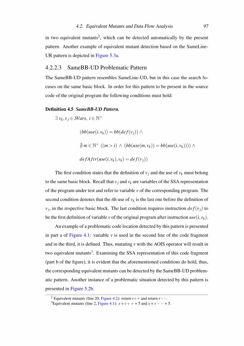
4.2. Equivalent Mutants and Data Flow Analysis 97
in two equivalent mutants2, which can be detected automatically by the present
pattern. Another example of equivalent mutant detection based on the SameLine-
UR pattern is depicted in Figure 5.3a.
4.2.2.3 SameBB-UD Problematic Pattern
The SameBB-UD pattern resembles SameLine-UD, but in this case the search fo-
cuses on the same basic block. In order for this pattern to be present in the source
code of the original program the following conditions must hold:
Definition 4.5 SameBB-UD Pattern.
∃ vk,v j ∈ SVars, i ∈ N+
(bb(use(i,vk)) = bb(de f (v j)) ∧
@ m ∈ N+ ((m > i) ∧ (bb(use(m,vk)) = bb(use(i,vk)))) ∧
de f A f tr(use(i,vk),vk) = de f (v j))
The first condition states that the definition of v j and the use of vk must belong
to the same basic block. Recall that v j and vk are variables of the SSA representation
of the program under test and refer to variable v of the corresponding program. The
second condition denotes that the ith use of vk is the last one before the definition of
v j, in the respective basic block. The last condition requires instruction de f (v j) to
be the first definition of variable v of the original program after instruction use(i,vk).
An example of a problematic code location detected by this pattern is presented
in part a of Figure 4.1: variable v is used in the second line of the code fragment
and in the third, it is defined. Thus, mutating v with the AOIS operator will result in
two equivalent mutants3. Examining the SSA representation of this code fragment
(part b of the figure), it is evident that the aforementioned conditions do hold, thus,
the corresponding equivalent mutants can be detected by the SameBB-UD problem-
atic pattern. Another instance of a problematic situation detected by this pattern is
presented in Figure 5.2b.
2 Equivalent mutants (line 20, Figure 4.2): return r++ and return r−−.3Equivalent mutants (line 2, Figure 4.1): x = v++ + 5 and x = v−− + 5.

4.2. Equivalent Mutants and Data Flow Analysis 98
4.2.2.4 SameBB-UR Problematic Pattern
As a special case of SameBB-UD, consider line 18 of Figure 4.2: it can be seen that
the application of AOIS will result in two equivalent mutants4. This is due to the
fact that variable x is never used between lines 18 and 20.
This problematic situation leads to the SameBB-UR problematic pattern,
which searches the source code of the original program for uses of variables that
belong to a basic block that can exit the program. More formally:
Definition 4.6 SameBB-UR Pattern.
∃ vk ∈ SVars, i ∈ N+
(isExit(bb(use(i,vk))) ∧
@ m ∈ N+ ((m > i) ∧ (bb(use(m,vk)) = bb(use(i,vk)))) ∧
@ v j ∈ SVars (de f A f tr(use(i,vk),vk) = de f (v j)))
The first condition necessitates the existence of a use inside a basic block that
can exit the program and the second one is the same as in the case of the SameBB-
UD pattern. The last condition requires the absence of any definitions of the used
variable after the using instruction.
Although the last condition is not required, its exclusion would cause instances
of the SameBB-UD pattern to be treated as instances of this particular one. For
the same reason, it is added in analogous cases of the Def-Def (DD) and Def-Ret
(DR) categories of patterns. An example of a problematic situation detected by this
pattern is illustrated in Figure 5.3b.
4.2.2.5 DifferentBB-UD Problematic Pattern
The DifferentBB-UD problematic pattern manages to detect partially equivalent
mutants and in specific cases, equivalent ones. This pattern searches for uses of
variables that can reach definitions by different paths, i.e. a variable is used in one
basic block and the same variable is defined in another one and these basic blocks
are connected via one or more paths.
4Equivalent mutants (line 18, Figure 4.2): r = x++ and r = x−−.

4.2. Equivalent Mutants and Data Flow Analysis 99
In order for this pattern to detect a problematic situation, the intermediate
nodes of at least one of the connecting paths must not include any uses or defi-
nitions of the respective variable. Such being the case, the change imposed on the
used variable (due to AOIS) cannot be revealed by targeting that path because the
variable is redefined prior to being used. More formally:
Definition 4.7 DifferentBB-UD Pattern.
∃ p ∈ Paths, vk,v j ∈ SVars, i ∈ N+
(reach(p,bb(use(i,vk)),bb(de f (v j))) ∧
@ m ∈ N+ ((m > i) ∧ (bb(use(m,vk)) = bb(use(i,vk)))) ∧
@ vq ∈ SVars (de f (vq) = de f A f tr(use(i,vk),vk)) ∧
de f A f tr( f rstIns(de f (v j)),v j) = de f (v j) ∧
@ vq ∈ SVars, n ∈ N+ (useB f r(de f (v j),v j) = use(n,vq)) ∧
useClr(p,vk) ∧
de fClr(p,vk))
where Paths is the set of paths of the CFG of the program under test.
Elaborating on these conditions, the first one requires the existence of a path
traversing the node that uses variable vk and the one that defines variable v j, i.e. the
nodes that use and define variable v of the original program. The next two conditions
refer to the basic block that contains the instruction of the ith use of variable vk (as
returned by use(i,vk)), hereafter referred to as the using basic block. The first one
states that the ith use of vk must be the last use of that variable in the using basic
block, i.e. there are no other uses of vk after instruction use(i,vk). The other one
prohibits the existence of a definition of variable v of the original program after the
ith use of v j (belonging to the using basic block).
The fourth and fifth conditions refer to the basic block that contains the in-
struction that defines variable v j (as returned by de f (v j)), hereafter referred to as
the defining basic block. The first of them states that de f (v j) is the first instruction
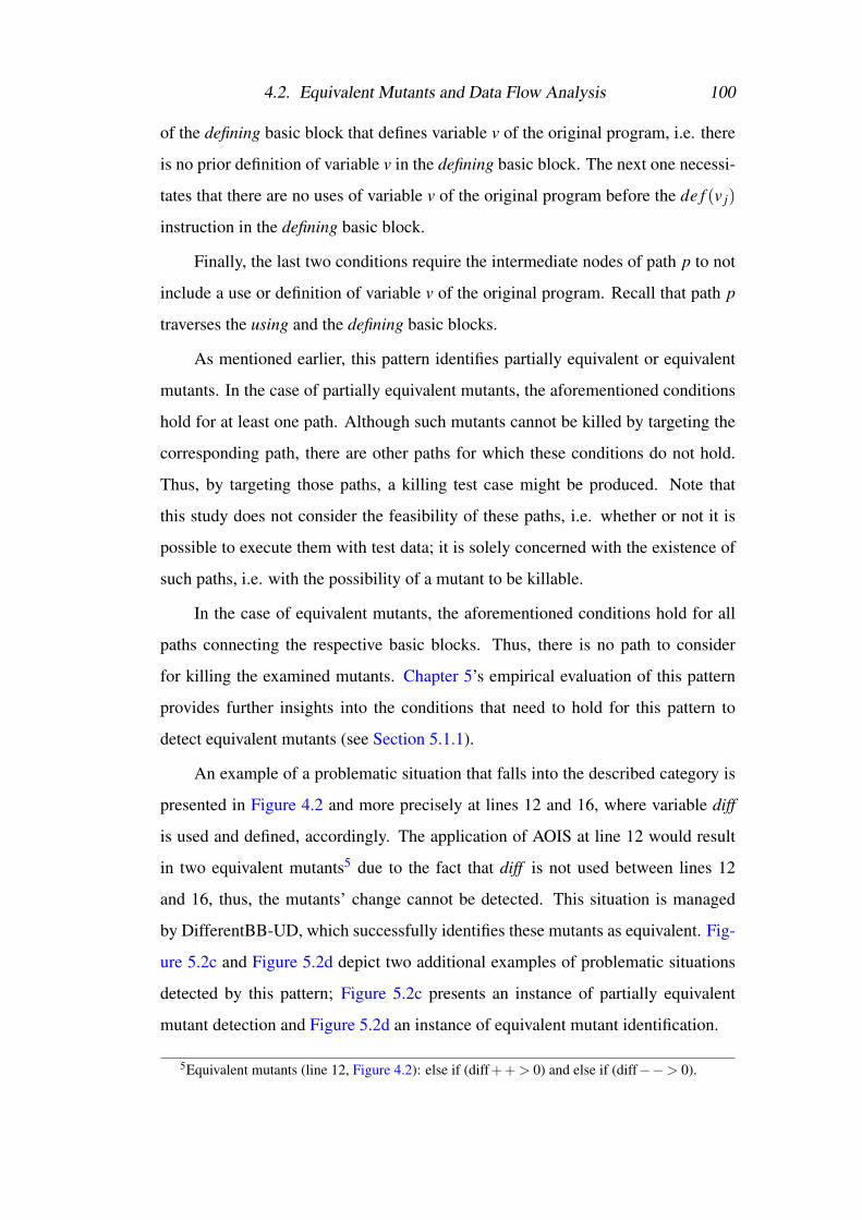
4.2. Equivalent Mutants and Data Flow Analysis 100
of the defining basic block that defines variable v of the original program, i.e. there
is no prior definition of variable v in the defining basic block. The next one necessi-
tates that there are no uses of variable v of the original program before the de f (v j)
instruction in the defining basic block.
Finally, the last two conditions require the intermediate nodes of path p to not
include a use or definition of variable v of the original program. Recall that path p
traverses the using and the defining basic blocks.
As mentioned earlier, this pattern identifies partially equivalent or equivalent
mutants. In the case of partially equivalent mutants, the aforementioned conditions
hold for at least one path. Although such mutants cannot be killed by targeting the
corresponding path, there are other paths for which these conditions do not hold.
Thus, by targeting those paths, a killing test case might be produced. Note that
this study does not consider the feasibility of these paths, i.e. whether or not it is
possible to execute them with test data; it is solely concerned with the existence of
such paths, i.e. with the possibility of a mutant to be killable.
In the case of equivalent mutants, the aforementioned conditions hold for all
paths connecting the respective basic blocks. Thus, there is no path to consider
for killing the examined mutants. Chapter 5’s empirical evaluation of this pattern
provides further insights into the conditions that need to hold for this pattern to
detect equivalent mutants (see Section 5.1.1).
An example of a problematic situation that falls into the described category is
presented in Figure 4.2 and more precisely at lines 12 and 16, where variable diff
is used and defined, accordingly. The application of AOIS at line 12 would result
in two equivalent mutants5 due to the fact that diff is not used between lines 12
and 16, thus, the mutants’ change cannot be detected. This situation is managed
by DifferentBB-UD, which successfully identifies these mutants as equivalent. Fig-
ure 5.2c and Figure 5.2d depict two additional examples of problematic situations
detected by this pattern; Figure 5.2c presents an instance of partially equivalent
mutant detection and Figure 5.2d an instance of equivalent mutant identification.
5Equivalent mutants (line 12, Figure 4.2): else if (diff++> 0) and else if (diff−−> 0).

4.2. Equivalent Mutants and Data Flow Analysis 101
4.2.2.6 DifferentBB-UR Problematic Pattern
A special case of DifferentBB-UD is the DifferentBB-UR problematic pattern,
which investigates pathogenic situations that arise when a use of a variable does
not reach another use, either because there is none or due to a statement that can
cause the program to exit, e.g. a return statement. In this case, the following
conditions need to hold for a code location to constitute a problematic situation:
Definition 4.8 DifferentBB-UR Pattern.
∃ p ∈ Paths, vk ∈ SVars, iε ∈ ExitIns, i ∈ N+
(reach(p,bb(use(i,vk)),bb(iε)) ∧
@ m ∈ N+ ((m > i) ∧ (bb(use(m,vk)) = bb(use(i,vk)))) ∧
@ vq ∈ SVars (de f A f tr(use(i,vk),vk) = de f (vq)) ∧
@ vq ∈ SVars (bb(de f (vq)) = bb(iε)) ∧
@ vq ∈ SVars, n ∈ N+ (bb(use(n,vq)) = bb(iε)) ∧
useClr(p,vk) ∧
de fClr(p,vk))
where ExitIns is the set of instructions that cause the program to exit.
These conditions are in accordance to the ones of the DifferentBB-UD prob-
lematic pattern. The first one requires the existence of a path connecting the basic
blocks that contain the use of variable vk and an instruction that forces the program
to exit. The next two state that at the basic block containing the use(i,vk) instruc-
tion, the ith use of vk is the last one and that there is no definition of variable v of
the original program after the corresponding use.
The following two conditions require that there are no definitions or uses of
variable v of the original program at the basic block containing instruction iε , re-
spectively. Finally, due to the last two conditions the intermediate nodes of path p
must not contain definitions or uses of variable v. Examples of partially equivalent

4.2. Equivalent Mutants and Data Flow Analysis 102
and equivalent mutant detection, based on this pattern, are presented in Figure 5.3c
and Figure 5.3d, respectively.
4.2.3 Def-Def (DD) and Def-Ret (DR) Categories of Patterns
As already mentioned, the Def-Def (DD) and Def-Ret (DR) categories of patterns
target equivalent mutants that are generated by mutation operators that affect vari-
able definitions. These categories are composed of the DD problematic pattern and
the SameBB-DR and DifferentBB-DR patterns, respectively.
4.2.3.1 DD Problematic Pattern
Th DD problematic pattern identifies problematic code locations based on subse-
quent definitions of a variable. Expanding on this, if a definition can reach another
definition of the same variable and there is no intermediate use of that variable, then
any change affecting the first definition cannot be revealed due to the fact that the
variable is redefined prior to being used.
Thus, mutants affecting that definition are bound to be partially equivalent, or
in specific cases, equivalent ones. It should be clarified that this category is not
restricted to a particular type of mutation operator; any mutation operator that can
affect the right part of an assignment statement (or a variable definition in general)
constitutes a possible target for the respective patterns.
An instance of a problematic situation that is detected by the present pattern
involves lines 3 and 13 of Figure 4.2, where variable M is defined. The only use
of the variable is at line 10 of basic block 4. Thus, mutants affecting the definition
of line 3 are bound to be partially equivalent for all paths from node 1 that include
node 6 and do not include node 4. Additional examples of partially equivalent and
equivalent mutant detection, based on this pattern, are presented in Figure 5.4a and
Figure 5.4b, respectively.
Recall that the equivalent mutant problem, in this study, is addressed for the
case of strong mutation, i.e. a mutant is considered equivalent if its output is the
same as the one of the original program for every possible input. Furthermore, it
should be mentioned that the partial equivalence of a mutant does not imply that the

4.2. Equivalent Mutants and Data Flow Analysis 103
mutant is equivalent; this knowledge should be utilised in order to avoid targeting
those paths that will not yield a killing test case for the examined mutant.
Unlike the UD and UR categories of patterns, DD is solely concerned with
problematic situations involving code locations that belong to different basic blocks.
Although, two definitions of the same variable can belong to the same basic block,
if these definitions are not accompanied with intermediate uses, they constitute a
problematic situation on their own. A more obscure problematic situation arises
when one definition of a variable can reach another one (of the same variable) along
a path that does not contain a node that uses that variable.
Mutants affecting such definitions would be partially equivalent and the corre-
sponding paths would never result in a test case that is able to kill the respective mu-
tants. Furthermore, if all paths traversing the basic blocks of the two definitions do
not include a node that uses the defined variable, then the above mentioned mutants
can be safely classified as equivalent. Thus, the identification of such problematic
cases will result in saving valuable resources, human and machine alike.
More formally, the necessary conditions that need to hold in order to detect the
described problematic situations are the following:
Definition 4.9 DD Pattern.
∃ p ∈ Paths, vk,v j ∈ SVars
(reach(p,bb(de f (vk)),bb(de f (v j))) ∧
@ vq ∈ SVars (de f A f tr(de f (vk),vk) = de f (vq)) ∧
@ vq ∈ SVars, n ∈ N+ (useA f r(de f (vk),vk) = use(n,vq)) ∧
de f A f tr( f rstIns(de f (v j)),v j) = de f (v j) ∧
@ vq ∈ SVars, n ∈ N+ (useB f r(de f (v j),v j) = use(n,vq)) ∧
useClr(p,vk) ∧
de fClr(p,vk))

4.2. Equivalent Mutants and Data Flow Analysis 104
These conditions are analogous to the ones of DifferentBB-UD, except that in
this case two definitions of a variable are considered and not a use and a definition.
The first condition requires the existence of a path traversing the node that defines
variable vk and the one that defines variable v j. The next two conditions state that
the de f (vk) instruction is the last definition of variable v of the original program in
the corresponding basic block and that there are no uses of v between the defining
instruction and the end of the basic block.
The remaining conditions are the same as in the case of the DifferentBB-UD
pattern and are restated here for completeness: they state that the de f (v j) instruction
is the first definition of variable v of the original program in the corresponding basic
block and that there are no uses of v between the first instruction of the basic block
and the defining instruction. Finally, the last two conditions require path p not to
contain any intermediate nodes that use or define variable v of the original program.
4.2.3.2 SameBB-DR Problematic Pattern
The patterns of the DR category resemble the previously described one, but instead
of searching for two definitions without an intermediate use, they search for a defi-
nition that cannot reach a use, either because there is none or due to a statement that
forces the program to exit.
This situation can manifest in the same or different basic blocks of a program
under test. In the former case, the SameBB-DR problematic pattern, the defining
statement belongs to a basic block that can exit the program. It should be mentioned
that in both cases the variable whose definition is affected must be local, i.e. it
should not be possible to access that variable after the exit of the corresponding
method (see also Section 5.1.4). In order for this pattern to become problematic the
following conditions must hold:
Definition 4.10 SameBB-DR Pattern.
∃ vk ∈ SVars
(isExit(bb(de f (vk))) ∧
@ vq ∈ SVars, n ∈ N+ (useA f r(de f (vk),vk) = use(n,vq)) ∧

4.2. Equivalent Mutants and Data Flow Analysis 105
@ v j ∈ SVars (de f A f tr(de f (vk),vk) = de f (v j)))
The first condition states that the instruction that defines variable vk belongs to
a basic block that can exit the program. The next one requires that there are no uses
of variable v of the original program after the corresponding defining instruction and
the last one prohibits the existence of another defining instruction of the considered
variable after instruction de f (vk).
4.2.3.3 DifferentBB-DR Problematic Pattern
The remaining pattern of the DR category, the DifferentBB-DR problematic pattern,
searches for problematic situations that manifest in different basic blocks, i.e. one
basic block which defines a variable is connected by at least one path (that does not
contain any intermediate nodes that use the corresponding variable) to a basic block
that can exit the program. More formally:
Definition 4.11 DifferentBB-DR Pattern.
∃ p ∈ Paths, vk ∈ SVars, iε ∈ ExitIns
(reach(p,bb(de f (vk)),bb(iε)) ∧
@ vq ∈ SVars (de f A f tr(de f (vk),vk) = de f (vq)) ∧
@ vq ∈ SVars, n ∈ N+ (useA f r(de f (vk),vk) = use(n,vq)) ∧
@ vq ∈ SVars (bb(de f (vq)) = bb(iε)) ∧
@ vq ∈ SVars, n ∈ N+ (bb(use(n,vq)) = bb(iε)) ∧
useClr(p,vk) ∧
de fClr(p,vk))
where ExitIns is the set of instructions that cause the program to exit.
These conditions are analogous to the ones of the DD problematic pattern. The
first one requires the existence of a path that traverses the basic block that contains
the definition of variable vk and one that can exit the program. The next two state
that, at the defining basic block, the de f (vk) instruction is the last one that defines

4.3. Empirical Study and Results 106
variable v of the original program and that there is no use of the variable in the
corresponding basic block after the definition.
The following two conditions require that there are no definitions or uses of
variable v of the original program at the node containing instruction iε , respectively.
Finally, the last two conditions require path p not to contain any intermediate nodes
that use or define variable v of the original program.
4.3 Empirical Study and ResultsThis study tackles the equivalent mutant problem by identifying problematic situ-
ations in the data flow information of the program under test that can lead to the
generation of equivalent or partially equivalent mutants. In order to investigate the
detection power of the introduced patterns as well as their presence in real-world
software, an empirical study was conducted based on a set of manually classified
mutants, hereafter referred to as the control mutant set. In the next subsections,
details about the experimental setup, the considered test subjects and the obtained
results are given.
4.3.1 Experimental Setup
4.3.1.1 Control Mutant Set and Subject Programs
This study is based on six Java test subjects6 which vary in size and application
domain. Table 4.2 presents the corresponding details. The first two columns of
the table depict the name of the studied test subjects and a short description of
their usage. The remaining columns introduce the corresponding lines of code and
the number of killable and equivalent mutants that were manually analysed for the
purposes of this study and comprise the control mutant set.
As can be seen from the table, the control mutant set is comprised of 747 man-
ually classified mutants, 663 of which are killable and 84 are equivalent ones. These
mutants were generated by the application of all method-level mutation operators
of the MUJAVA (version 3) mutation testing framework [19, 163].
6Note that the same test subjects and manually analysed mutants were utilised in the study pre-sented in Chapter 6.

4.3. Empirical Study and Results 107
Table 4.2: Subject Program Details.
Program Description LOC Killable EquivalentBisect Square root calculation 36 40 4Commons Various utilities 19,583 110 28Joda-time Date and time utilities 25,909 42 4Pamvotis WLAN simulator 5,149 142 10Triangle Returns triangle type 32 183 30Xstream XML object serialisation 16,791 146 8Total 67,500 663 84
Since this study targets the equivalent mutant problem and the introduced pat-
terns do not yield false positive results, only the equivalent mutants of the control
mutant set are utilised. Studying the respective killable ones would be valuable in
the case of partially equivalent mutants. Note that Chapter 5 presents more infor-
mation about this kind of mutants.
4.3.1.2 Experimental Procedure
In order to investigate the detection power of the introduced problematic patterns,
the mutated location of each equivalent mutant was manually investigated in order
to determine whether or not this particular location can be identified as problematic
by the proposed patterns, i.e. if the conditions of at least one of the introduced
patterns are satisfied.
Note that the manual investigation is performed solely for the purposes of this
experiment. The proposed data flow patterns can be incorporated into an automated
framework and, thus, can facilitate the automated detection of equivalent mutants.
Chapter 5 presents such a framework.
4.3.2 Empirical Findings
The empirical results of the conducted study are presented in Table 4.3. The second
and third columns of the table present the number of the manually detected equiva-
lent mutants and the number of these mutants that can be automatically detected by
the application of the proposed data flow patterns per test subject, respectively. The
last column presents the achieved reduction in the number of mutants that have to
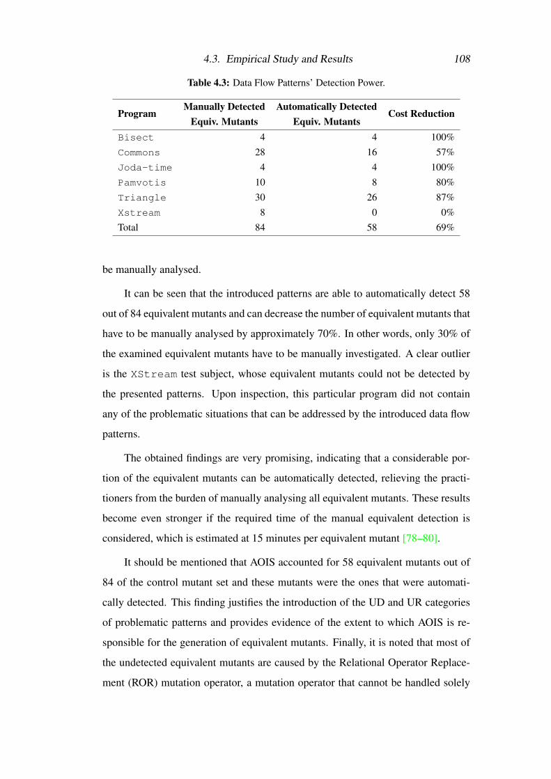
4.3. Empirical Study and Results 108
Table 4.3: Data Flow Patterns’ Detection Power.
ProgramManually Detected Automatically Detected
Cost ReductionEquiv. Mutants Equiv. Mutants
Bisect 4 4 100%Commons 28 16 57%Joda-time 4 4 100%Pamvotis 10 8 80%Triangle 30 26 87%Xstream 8 0 0%Total 84 58 69%
be manually analysed.
It can be seen that the introduced patterns are able to automatically detect 58
out of 84 equivalent mutants and can decrease the number of equivalent mutants that
have to be manually analysed by approximately 70%. In other words, only 30% of
the examined equivalent mutants have to be manually investigated. A clear outlier
is the XStream test subject, whose equivalent mutants could not be detected by
the presented patterns. Upon inspection, this particular program did not contain
any of the problematic situations that can be addressed by the introduced data flow
patterns.
The obtained findings are very promising, indicating that a considerable por-
tion of the equivalent mutants can be automatically detected, relieving the practi-
tioners from the burden of manually analysing all equivalent mutants. These results
become even stronger if the required time of the manual equivalent detection is
considered, which is estimated at 15 minutes per equivalent mutant [78–80].
It should be mentioned that AOIS accounted for 58 equivalent mutants out of
84 of the control mutant set and these mutants were the ones that were automati-
cally detected. This finding justifies the introduction of the UD and UR categories
of problematic patterns and provides evidence of the extent to which AOIS is re-
sponsible for the generation of equivalent mutants. Finally, it is noted that most of
the undetected equivalent mutants are caused by the Relational Operator Replace-
ment (ROR) mutation operator, a mutation operator that cannot be handled solely

4.4. Summary 109
by data flow information.
4.4 SummaryThis chapter introduced and described formally nine data flow patterns that are able
to automatically detect equivalent and partially equivalent mutants. For each pat-
tern, the specific conditions, between variable definitions and uses, that need to hold
for the existence of the respective problematic situations in the source code of the
program under test are defined.
The Static Single Assignment (SSA) intermediate representation of the exam-
ined program was utilised for the purposes of the patterns’ definition. The salient
feature of this representation is that each variable is assigned exactly once, thus,
it facilitates powerful code analysis and a clearer definition of the aforementioned
conditions.
An empirical study, conducted on approximately 800 manually analysed mu-
tants from several open source projects, investigated the detection power of the pro-
posed data flow patterns and their existence in real-world software. The obtained
results revealed that the introduced patterns were indeed present in such software
and were able to detect approximately 70% of the examined equivalent mutants,
thus, considerably reducing mutation’s manual effort.
The next chapter investigates further the proposed data flow patterns. An au-
tomated tool, named Mutants’ Equivalence Discovery (MEDIC), that incorporates
these patterns is implemented and its effectiveness and efficiency are empirically
evaluated.

Chapter 5
A Static Analysis Framework for Equivalent
Mutant Identification
It is generally known that the equivalent mutant problem impedes the adoption of
mutation testing in practice. This situation is exacerbated further by its undecidable
nature. Thus, the need to introduce automated solutions, albeit partial, to tackle this
problem becomes apparent. In view of this, this chapter introduces a static anal-
ysis framework for equivalent mutant identification, named Mutants’ Equivalence
Discovery (MEDIC).
MEDIC implements the data flow patterns introduced in Chapter 4. The pres-
ence of these patterns in the source code of the program under test was found to
lead to the generation of equivalent and partially equivalent mutants. Recall that a
partially equivalent mutant is equivalent to the original program for specific paths
and, as a consequence, these paths cannot produce killing test cases for the corre-
sponding mutant. Despite this fact, partially equivalent mutants can be killable.
A salient characteristic of the utilised patterns is that they are determined stat-
ically, i.e. they can be incorporated into mutation testing frameworks to weed out
a portion of the total equivalent mutants before their generation, without the need
to execute the considered mutants. Thus, their utilisation would greatly boost the
frameworks’ efficiency. The empirical assessment of MEDIC evaluates this state-
ment and investigates further the detection power of the implemented patterns.
Apart from examining MEDIC’s effectiveness and efficiency, this chapter also
explores the cross-language nature of the aforementioned patterns, i.e. whether or

5.1. Background: Problematic Data Flow Patterns 111
not they can detect equivalent and partially equivalent mutants in programs written
in different programming languages. Finally, the killability of the detected partially
equivalent mutants and the difficulty in performing such a task were also investi-
gated.
In summary, the present chapter makes the following contributions:
1. An automated framework, named Mutants’ Equivalence Discovery (MEDIC)
which implements the data flow patterns introduced in Chapter 4 and is able
to detect equivalent and partially equivalent mutants in different programming
languages.
2. An empirical study, based on 1,287 manually analysed mutants from real-
world projects, which investigates MEDIC’s detection power, performance
and cross-language nature.
3. Insights into the nature of partially equivalent mutants and the difficulty in
killing them.
The rest of this chapter is organised as follows. Section 5.1 succinctly describes
the implemented data flow patterns in conjunction with examples belonging to the
examined test subjects, in order for this chapter to be self-contained. Section 5.2
presents the implementation details of MEDIC and Section 5.3 the conducted em-
pirical study. Next, Section 5.4 describes the obtained experimental results and
discusses possible threats to validity. Finally, Section 5.5 concludes this chapter,
summarising key findings.
5.1 Background: Problematic Data Flow PatternsChapter 4 introduced several data flow patterns that detect source code locations
capable of generating equivalent mutants. These patterns examine the data flow in-
formation of the program under test. The underlying analysis is based on the Static
Single Assignment (SSA) intermediate representation [159, 160]; a form utilised by
modern compilers for the internal representation of the input program.

5.1. Background: Problematic Data Flow Patterns 112
The basic characteristic of the SSA representation is that each variable of the
program under test is assigned exactly once. Essentially, for each assignment to a
variable, that variable is uniquely named and all its uses, reached by that assignment,
are appropriately renamed [162]. An example of this representation is illustrated in
Figure 5.1.
The first part of the figure presents a portion of the source code of the
uncapitalize method of the Commons test subject1 and the second part its
SSA representation, as obtained by the T. J. Watson Libraries for Analysis (WALA)
framework [164], a program analysis tool utilised by MEDIC. The lines of each part
of the figure are numbered in such a way that directly relates the source code with
its SSA representation: the SSA representation of line 1 of the source code (part a)
is line 1 of part b, for line 5 of part a, the corresponding line is part b’s line 5 and so
on.
By examining this figure, it becomes clear that each variable is uniquely named
in the SSA representation based on its assignments in the source code and that its
uses are also renamed appropriately. Section 5.2 elaborates on this example and
describes the WALA and MEDIC frameworks in more detail.
The considered data flow patterns can lead to the detection of equivalent and
partially equivalent mutants. A partially equivalent mutant is a mutant that is equiv-
alent to the original program only for a specific set of paths, whereas an equivalent
one is equivalent to the original program for all paths.
The identification of partially equivalent mutants is considered valuable due
to the discovery of the subset of paths that will not yield a killing test case for the
corresponding mutant. The present work empirically studies the concept of partially
equivalent mutants and discusses the corresponding findings in Section 5.4.
5.1.1 Use-Def (UD) Category of Patterns
As mentioned in Section 4.2.2, the Use-Def (UD) category of patterns targets equiv-
alent mutants that are due to mutation operators that insert the post-increment or
decrement arithmetic operators or other similar operators. The patterns belonging
1Apache Commons Lang project (https://commons.apache.org).
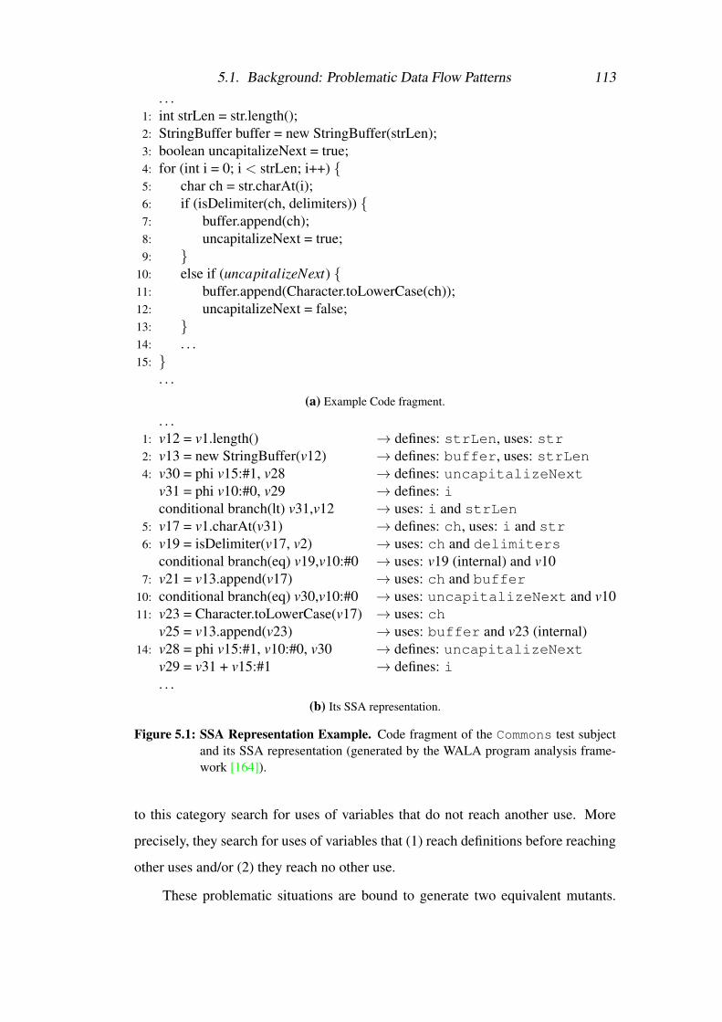
5.1. Background: Problematic Data Flow Patterns 113. . .
1: int strLen = str.length();2: StringBuffer buffer = new StringBuffer(strLen);3: boolean uncapitalizeNext = true;4: for (int i = 0; i < strLen; i++) {5: char ch = str.charAt(i);6: if (isDelimiter(ch, delimiters)) {7: buffer.append(ch);8: uncapitalizeNext = true;9: }
10: else if (uncapitalizeNext) {11: buffer.append(Character.toLowerCase(ch));12: uncapitalizeNext = false;13: }14: . . .15: }
. . .(a) Example Code fragment.
. . .1: v12 = v1.length() → defines: strLen, uses: str2: v13 = new StringBuffer(v12) → defines: buffer, uses: strLen4: v30 = phi v15:#1, v28 → defines: uncapitalizeNext
v31 = phi v10:#0, v29 → defines: iconditional branch(lt) v31,v12 → uses: i and strLen
5: v17 = v1.charAt(v31) → defines: ch, uses: i and str6: v19 = isDelimiter(v17, v2) → uses: ch and delimiters
conditional branch(eq) v19,v10:#0 → uses: v19 (internal) and v107: v21 = v13.append(v17) → uses: ch and buffer
10: conditional branch(eq) v30,v10:#0 → uses: uncapitalizeNext and v1011: v23 = Character.toLowerCase(v17) → uses: ch
v25 = v13.append(v23) → uses: buffer and v23 (internal)14: v28 = phi v15:#1, v10:#0, v30 → defines: uncapitalizeNext
v29 = v31 + v15:#1 → defines: i. . .
(b) Its SSA representation.
Figure 5.1: SSA Representation Example. Code fragment of the Commons test subjectand its SSA representation (generated by the WALA program analysis frame-work [164]).
to this category search for uses of variables that do not reach another use. More
precisely, they search for uses of variables that (1) reach definitions before reaching
other uses and/or (2) they reach no other use.
These problematic situations are bound to generate two equivalent mutants.

5.1. Background: Problematic Data Flow Patterns 114
Consider, for instance, the use of variable ch at line 11 of Figure 5.1. This variable
constitutes a valid target for the Arithmetic Operator Insertion Short-cut (AOIS)
mutation operator of the MUJAVA framework. Furthermore, note that the use of line
11 will either reach another use only after a definition of the same variable or will
not reach another use (in the case the for block exits).
Taking these facts into account, it becomes clear that the application of the
post-increment and decrement operators to this variable, i.e. the application of
AOIS, will result in two equivalent mutants. Analogous cases are handled by the
patterns of this category, which are briefly described subsequently:
• SameLine-UD Problematic Pattern. The SameLine-UD problematic pat-
tern detects solely equivalent mutants that affect a variable that is being used
and defined at the same statement. In this particular case, the changes in-
duced by the post-increment and decrement operators can never be distin-
guished. Figure 5.2a presents an example from the classify method of
the Triangle test subject: the application of AOIS at line 29 will generate
two equivalent mutants, denoted by the symbol ∆, affecting variable trian.
The SameLine-UD pattern discovers this problematic source code location
by identifying the use and the definition of trian at the corresponding line, as
highlighted in the figure.
• SameBB-UD Problematic Pattern. This pattern also detects solely equiva-
lent mutants, but in this case the use of the variable and its definition belong
to the same basic block. Thus, SameBB-UD searches for basic blocks that
contain uses and definitions of the same variable and the use precedes the
definition with no intermediate uses. The application of AOIS to such a case
will inevitably lead to the generation of equivalent mutants. An example of
this problematic situation belonging to the wrap method of the Commons
test subject, is depicted in Figure 5.2b, where variable offset, which consti-
tutes a valid target for AOIS, is used at line 56 and is later defined at line 57.
This situation is detected by SameBB-UD, leading to the discovery of the two
equivalent mutants depicted in the figure.

5.1. Background: Problematic Data Flow Patterns 115
. . .28: if (a == c) {29: trian = trian + 2;
∆ . . . trian++ . . .∆ . . . trian−− . . .
30: }. . .(a) Triangle: SameLine-UD – Equiv.
. . .55: else {56: . . . (str.substring( offset ));
∆ . . . (offset++));∆ . . . (offset−−));
57: offset = inputLineLength;58: }
. . .
(b) Commons: SameBB-UD – Equiv.
. . .30: while (ABS(diff) > mEpsilon) {31: if (diff < 0) {32: m = x; // BB:433: x = ( M + x) / 2;
∆ . . . M++ . . .∆ . . . M−− . . .
34: }35: else if (diff > 0) {36: M = x; // BB:637: x = (m + x) / 2;38: }39: diff = x * x - N;40: }
. . .(c) Bisect: DifferentBB-UD – Partially Eq.
117: for (; i < length; i++) {118: char c = name.charAt(i);119: if (. . .) {120: . . .122: }123: else if (. . .) {124: . . .125: }126: else {127: result.append( c );
∆ . . . (c++);∆ . . . (c−−);
128: }129: }
. . .(d) XStream: DifferentBB-UD – Equiv.
Figure 5.2: Problematic Situations Detected by the Use-Def (UD) Category of Patterns.Each part presents a code fragment of a studied test subject, the name of thediscovering pattern and the type of the detected mutants (denoted by the ∆
symbol).
• DifferentBB-UD Problematic Pattern. The DifferentBB-UD pattern de-
tects partially equivalent mutants and in specific cases equivalent ones. This
pattern searches for uses and definitions of variables between different basic
blocks. More precisely, it searches for uses of variables at one basic block
(the using basic block) that can reach a definition of that variable at another
basic block (the defining basic block), without other intermediate uses or def-
initions. Such being the case, a path connecting the using and defining basic
blocks cannot yield a killing test case for the considered mutants (ones gener-
ated by the AOIS mutation operator). Thus, these mutants can be identified as

5.1. Background: Problematic Data Flow Patterns 116
partially equivalent for this specific path. An instance of this case is illustrated
in Figure 5.2c. This figure presents a code fragment of the sqrt method of
the Bisect test subject. It can been seen that variable M is used at basic
block 4 and is defined at basic block 6. Thus, a path that contains these ba-
sic blocks with that particular order and no other uses of M cannot yield a
killing test case for the mutants depicted in the figure. Apart from detect-
ing partially equivalent mutants, DifferentBB-UD can also detect equivalent
ones: in this case, (1) the previously stated conditions must hold for all paths
connecting the using and defining basic blocks and (2) no path should exist
that connects the using basic block with another one that uses the respective
variable and does not include an intermediate basic block that defines the cor-
responding variable. It should be mentioned that this last condition was not
included in the original definition of this pattern and was added to address a
corner case belonging to a studied test subject. Figure 5.2d, which depicts
a code fragment of the decodeName method of the XStream test subject,
presents an instance of equivalent mutant detection. The problematic pattern
resides in lines 127 and 118. At the former, variable c is used and at the lat-
ter it is defined. The application of AOIS at this specific code location will
lead to the generation of two equivalent mutants, which are discovered by the
DifferentBB-UD pattern. Another example of equivalent detection based on
this pattern was presented at the beginning of this subsection.
The aforementioned patterns search for uses of variables that can reach a def-
inition. As a special case, the Use-Ret (UR) category of patterns searches for uses
that do not reach another use.
5.1.2 Use-Ret (UR) Category of Patterns
The Use-Ret (UR) family of patterns, introduced in Section 4.2.2, searches for uses
of variables that do not reach another use. Thus, the application of the AOIS muta-
tion operator at these specific code locations will lead to the generation of equivalent
or partially equivalent mutants. This category includes three patterns that are anal-
ogous to the previously presented ones.

5.1. Background: Problematic Data Flow Patterns 117
. . .187: if (divisor == 1) {188: return this;189: }190: return mins(getVal()/ divisor );
∆ . . . /divisor++);∆ . . . /divisor−−);. . .
(a) Joda-time: SameLine-UR – Equiv.
. . .83: if (position != -1) {84: . . . rmElementAt( position );
∆ . . . (position++);∆ . . . (position−−);
85: return true;86: } else {
. . .88: }
(b) Pamvotis: SameBB-UR – Equiv.
. . .214: for (. . . ; i < isize; i++) {215: if ( ch == delimiters[i]) {
∆ (ch++ . . . )∆ (ch−− . . . )
216: return true;217: }218: }219: return false;
. . .(c) Commons: DifferentBB-UR – Partially Eq.
. . .49: else {50: if (tr == 3 && b + c>a) {
∆ . . . && b++ . . .∆ . . . && b−− . . .
51: return ISOSCELES;52: }53: }
. . .55: return INVALID;
(d) Triangle: DifferentBB-UR – Equiv.
Figure 5.3: Problematic Situations Detected by the Use-Ret (UR) Category of Patterns.Each part presents a code fragment of a studied test subject, the name of thediscovering pattern and the type of the detected mutants (denoted by the ∆
symbol).
• SameLine-UR Problematic Pattern. This pattern targets equivalent mutants
that relate to problematic situations where a variable is used at an exiting
statement, e.g. a return statement. An example of such a case is present in
Figure 5.3a, which illustrates a code fragment of the dividedBy method of
the Joda-time test subject. It can be seen that variable divisor is used at the
return statement of line 190; the application of AOIS at this particular line
will result in two equivalent mutants (depicted in the figure) that are detected
by this pattern.
• SameBB-UR Problematic Pattern. The SameBB-UR pattern is analogous
to the SameBB-UD one, but instead of searching for uses of a variable that
coexist with definitions of the same variable inside a basic block, it searches

5.1. Background: Problematic Data Flow Patterns 118
for basic blocks that contain exiting statements and include uses of variables
that do not reach other uses. An instance of this situation is illustrated in
Figure 5.3b, which presents a code fragment of the removeSource method
of the Pamvotis test subject. It can be seen that the highlighted use of
variable position does not reach another use before the return statement of
line 85. Thus, the application of the AOIS mutation operator will generate
two equivalent mutants that are discovered by this pattern.
• DifferentBB-UR Problematic Pattern. This pattern constitutes a special
case of the DifferentBB-UD one in that it searches for uses of variables at
a basic block that can reach an exiting basic block without any intermediate
uses or definitions. In this particular circumstance, the application of AOIS
can lead to the generation of partially equivalent mutants or equivalent ones.
An example of the former case is depicted in Figure 5.3c. This code frag-
ment belongs to the isDelimiter method of the Commons test subject. It
can be seen that the only use of variable ch is at line 215 which lies inside
a for block. Consequently, any path that does not contain more than one
loops, i.e. more than one uses of this variable, cannot produce killing test
cases for the AOIS mutants. The DifferentBB-UR pattern identifies this fact
and marks this code location as problematic and the corresponding mutants
as partially equivalent. Figure 5.3d presents an instance of a code location
that will generate equivalent mutants. This figure illustrates a code fragment
of the classify method of the Triangle test subject. It can be seen that
variable b is used at line 50 and has no other uses after this line. Thus, the
mutants created by the insertion of the post-increment and decrement arith-
metic operators can never be killed. The DifferentBB-UR pattern discovers
this problematic situation.
5.1.3 Def-Def (DD) Category of Patterns
The Def-Def (DD) category of patterns, presented in Section 4.2.3, targets prob-
lematic situations that are caused by definitions of variables instead of uses. This

5.1. Background: Problematic Data Flow Patterns 119
. . .76: int position = -1;
∆ . . . = 1;77: for (int i = 0; . . . ; i++) {78: if (. . .) {79: position = i;80: break;81: }82: }
. . .(a) Pamvotis: DD – Partially Eq.
1089: float nAifsd = sifs + 2 * slot;∆ . . . / slot;
1090: switch (ac) {1091: case 1 :1092: { . . .1095: nAifsd = sifs + aifs1 * slot;1096: . . .1097: }
. . .1115: default :1116: { . . .1119: nAifsd = sifs + aifs0 * slot;1120: . . .1121: }
(b) Pamvotis: DD – Equiv.
Figure 5.4: Problematic Situations Detected by the Def-Def (DD) Category of Patterns.Each part presents a code fragment of a studied test subject, the name of thediscovering pattern and the type of the detected mutants (denoted by the ∆
symbol).
constitutes the main difference between this category and the aforementioned ones.
The only pattern that belongs to this family is the DD problematic pattern.
• DD Problematic Pattern. This pattern detects problematic situations that
arise from the existence of two consecutive definitions of a variable, belong-
ing to different basic blocks, with no intermediate uses. Such being the case,
any mutation operator that changes the first definition is bound to generate
partially equivalent mutants or equivalent ones. In the former situation, the
two definitions must be reached by at least one path with no intermediate
uses – these paths cannot produce a killing test case for the respective mu-
tants. In the latter case, every path reaching the first definition must reach a
second one (with no intermediate uses), thus, the change induced by mutation
operators affecting the first definition cannot be discerned. Examples of such
mutation operators are: the Arithmetic Operator Deletion Unary (AODU) and
the Arithmetic Operator Replacement Binary (AORB) mutation operators of
the MUJAVA framework. An instance of a code location that will generate
partially equivalent mutants is presented in Figure 5.4a. This code fragment

5.1. Background: Problematic Data Flow Patterns 120
belongs to the removeSource method of the Pamvotis test subject. It
can be seen that variable position is defined twice, at lines 76 and 79 respec-
tively, and there is no use of that variable prior to the second definition. Due to
the fact that these two definitions can be reached by at least one path and there
is no use between them, it can be concluded that mutants affecting the defini-
tion of line 76 are partially equivalent. The depicted mutant, produced by the
AODU mutation operator which deletes unary arithmetic operators, falls into
this category. The DD pattern can also detect equivalent mutants: Figure 5.4b
illustrates an example belonging to the addNode method of the Pamvotis
test subject. In this code fragment, variable nAifsd, which is defined at line
1089, is later redefined at every case block and at the default block of
the switch statement, without any intermediate uses. Consequently, every
path reaching the definition of line 1089 will definitely reach a second one.
The DD pattern identifies this fact and reports that the mutants affecting the
right expression of this definition are equivalent ones. An instance of such
a mutant, generated by the AORB mutation operator which replaces binary
arithmetic operators, is presented in the figure.
5.1.4 Def-Ret (DR) Category of Patterns
The Def-Ret (DR) category of patterns, introduced in Section 4.2.3, constitutes a
special case of the aforementioned one. The patterns of this category search for
definitions of variables that do not reach a use. In such a case, the induced change of
the mutants affecting that particular definition is indistinguishable. Unfortunately,
this implies the existence of unused variables in the program under test, which is
or should be scarce in a real-world application. The empirical assessment of these
patterns showed no instances of equivalent mutant detection (see Section 5.4 for
more details), thus, their description is not accompanied by appropriate source code
examples.
• SameBB-DR Problematic Pattern. The SameBB-DR pattern searches for
definitions of variables at a basic block that contains (1) an exiting statement
and (2) no use of those variables between the considered definition and the

5.1. Background: Problematic Data Flow Patterns 121. . .
41: r = x;42: mResult = r; // mResult is not a local variable
∆ . . . = -r;43: return r;
Figure 5.5: SameBB-DR Pattern: Handling Non-local Variables. A detected problem-atic situation based on the original definition of SameBB-DR. The depictedmutant (denoted by the ∆ symbol) is killable because mResult is not a localvariable. The refined definition of this pattern rectifies this situation.
exiting statement. It is obvious that such a case will generate equivalent mu-
tants. The empirical evaluation of this pattern revealed an additional require-
ment: (3) it should not be possible to access the variable whose definition is
affected after the exit of the corresponding method, e.g. the case of a non-
local variable. Consider for example Figure 5.5. This figure presents a code
fragment of the Bisect test subject. According to the original definition of
the SameBB-DR pattern, the highlighted definition of variable mResult will
be detected as a problematic code location that will generate equivalent mu-
tants. Upon closer inspection, it becomes apparent that these mutants can be
easily killed by examining the value of mResult after the end of the respective
method since it is not a local variable. The newly added requirement refines
SameBB-DR’s definition and rectifies the aforementioned situation.
• DifferentBB-DR Problematic Pattern. The DifferentBB-DR pattern
searches for definitions of variables at one basic block that reach an exit-
ing basic block, without any intermediate uses. This pattern can detect both
equivalent and partially equivalent mutants. In the first case, every path reach-
ing the considered definition must also reach an exiting basic block (with no
intermediate uses) and in the second one, at least one such path must exist
between the defining and exiting basic blocks. The empirical evaluation of
this pattern revealed no cases of equivalent mutant detection, similarly to
the SameBB-DR one, although it did reveal instances of partially equivalent
mutants.
5.2. MEDIC – Mutants’ Equivalence DIsCovery 122
5.2 MEDIC – Mutants’ Equivalence DIsCoveryThe primary focus of this chapter is the empirical evaluation of the problematic
patterns described in Chapter 4. To fulfil this, an automated framework, named Mu-
tant’s Equivalence Discovery (MEDIC), incorporating these patterns has been im-
plemented. MEDIC is written in the Jython programming language and leverages
several frameworks to perform its analyses. MEDIC’s components and implemen-
tation details are presented in the following sections.
MEDIC utilises the Static Single Assignment (SSA) form [159, 160] of a pro-
gram under test to perform its analysis. As mentioned at the beginning of Sec-
tion 5.1, the SSA form is an internal representation of a program whose basic char-
acteristic is that every variable has exactly one definition. MEDIC obtains such a
representation by leveraging the T. J. Watson Libraries for Analysis (WALA) frame-
work [164].
5.2.1 T. J. Watson Libraries for Analysis (WALA)
The WALA framework [164] is a static analysis tool for the Java and the JavaScript
programming languages. It can perform various analyses, control and data flow
alike. The following information is obtained by the application of WALA to the
program under test:
• SSA form of the artefact under test. WALA transforms the source code of
the input program into SSA instructions which form its SSA representation.
An instance of this transformation was depicted in Figure 5.1, which presents
a code fragment of the Commons test subject, along with the generated SSA
instructions. WALA applies several optimisations to the transformation pro-
cess. Most notably, it constructs pruned SSA forms [165] and employs copy
propagation [166]. Note that these optimisations are not a prerequisite for the
application of MEDIC. In fact, their employment prevents MEDIC from dis-
covering all problematic source code locations that the implemented patterns
would have in theory2.
2This results in MEDIC’s missing 7 equivalent mutants, cf. Table 5.3.

5.2. MEDIC – Mutants’ Equivalence DIsCovery 123
• Control Flow Graph of the SSA form. WALA divides the produced SSA
instructions into basic blocks, creating an SSA-based control flow graph.
MEDIC utilises this graph to examine the requirements of each implemented
pattern.
• Definitions and uses per SSA instruction. Typically, each SSA instruction
has a single definition and one or more uses. These definitions and uses re-
fer to variables in the SSA representation of the program under test and do
not necessarily map to ones in its source code. By examining the second
part of Figure 5.1, it becomes evident that even though the uses of the SSA
form match the ones of the corresponding code fragment (first part of the fig-
ure), the definitions do not. For instance, the definitions of lines 3 and 4 of
the source code do not directly correspond to appropriate ones in the SSA
form. Instead, these definitions appear as phi statements, or more precisely
as φ -functions, in the SSA representation. A φ -function is a special form of
an assignment which is added to the SSA representation of a program when
there are variables in its source code that are defined along two converging
paths [167]. In other words, two or more definitions of a variable in the source
code can reach the same use of that variable via different paths. Such a case is
present in Figure 5.1 where variable i is defined at the initialisation expression
of the for statement (i = 0) and it is redefined at its increment expression
(i++). These two definitions both reach the use of i at the termination expres-
sion of the for statement (i < strLen) via different paths. Thus, WALA
adds an appropriate φ -function (v31 = phi v10:#0,v29) before that par-
ticular use in the produced SSA representation. A similar situation pertaining
to the definitions of variable uncapitalizeNext (lines 3, 8, 12) is treated
analogously, as shown in the figure.
5.2.2 MEDIC’s Implementation Details
The previously described data form the basis for the operation of MEDIC. In order
to increase MEDIC’s extensibility, these data are not used in their raw format. In-

5.2. MEDIC – Mutants’ Equivalence DIsCovery 124
stead, a custom data model has been developed that encapsulates all the necessary
information for MEDIC’s operation.
The main advantage of such an approach is that MEDIC is decoupled from the
internal mechanics of WALA and can leverage other program analysis frameworks
that can potentially support different programming languages. Due to the fact that
the data to be modelled were graph-centric, i.e. interconnected basic blocks contain-
ing uses and definitions of variables, the utilisation of graph databases was deemed
appropriate. In particular, MEDIC utilises the NEO4J graph database [168].
Graph databases model the underlying data based on nodes and relationships
which can have properties. A property augments the corresponding model with
additional information pertinent to the respective node or relationship. MEDIC
defines two kinds of nodes in its data model, the Basic Block nodes and the
Variable ones, and introduces three types of relationships, the goes relationship
that connects two Basic Block nodes and the uses and defines relationships
that connect a Basic Block node with a Variable one.
Figure 5.6 presents an illustrative example of the aforementioned data model
that belongs to the Bisect test subject. By examining this figure, it becomes
apparent that the developed model clearly captures both control and data flow infor-
mation of basic block bb2. This figure also presents the properties that individual
nodes and relationships can possess. For instance, a Basic Block node can con-
tain only one property, the id property, whereas a Variable node can contain
more. Regarding the corresponding relationships, uses and defines include
similar properties and the goes relationship includes none.
The information described by the previously presented data model suffices for
the application of MEDIC, i.e. MEDIC examines this information to discover prob-
lematic code locations in the source code of the program under test that can gener-
ate equivalent or partially equivalent mutants. Note that even though this analysis
is based on the SSA representation of the examined program, the discovered code
locations refer to its source code.
In the following subsections, the generic algorithm that MEDIC employs for
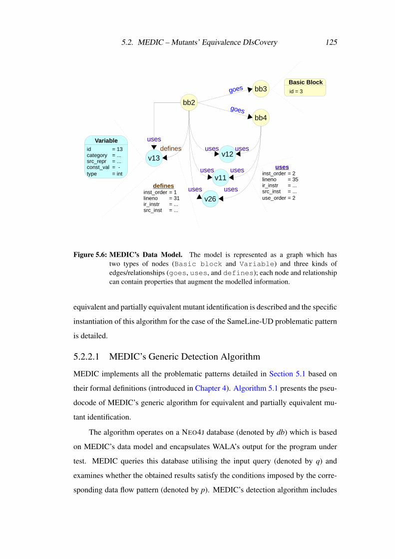
5.2. MEDIC – Mutants’ Equivalence DIsCovery 125
bb2
bb3
v12
v26
v11
uses
v13
bb4
uses
uses
uses
uses
uses
goes
goes
Basic Block
id = 3
Variableid = 13category = ... src_repr = ...const_val = -type = int
definesinst_order = 1lineno = 31ir_instr = ...src_inst = ...
usesinst_order = 2lineno = 35ir_instr = ...src_inst = ...use_order = 2
defines
uses
Figure 5.6: MEDIC’s Data Model. The model is represented as a graph which hastwo types of nodes (Basic block and Variable) and three kinds ofedges/relationships (goes, uses, and defines); each node and relationshipcan contain properties that augment the modelled information.
equivalent and partially equivalent mutant identification is described and the specific
instantiation of this algorithm for the case of the SameLine-UD problematic pattern
is detailed.
5.2.2.1 MEDIC’s Generic Detection Algorithm
MEDIC implements all the problematic patterns detailed in Section 5.1 based on
their formal definitions (introduced in Chapter 4). Algorithm 5.1 presents the pseu-
docode of MEDIC’s generic algorithm for equivalent and partially equivalent mu-
tant identification.
The algorithm operates on a NEO4J database (denoted by db) which is based
on MEDIC’s data model and encapsulates WALA’s output for the program under
test. MEDIC queries this database utilising the input query (denoted by q) and
examines whether the obtained results satisfy the conditions imposed by the corre-
sponding data flow pattern (denoted by p). MEDIC’s detection algorithm includes

5.2. MEDIC – Mutants’ Equivalence DIsCovery 126
Algorithm 5.1 MEDIC’s Generic Algorithm for Equivalent and Partially EquivalentMutant Identification.
Let p represent a problematic data flow patternLet q represent a Cypher query for pLet db represent a NEO4J database modelling WALA’s output
1: function EQUIVALENTMUTANTDIAGNOSIS(q, p, db)2: qres← execute(q,db)3: foreach r ∈ qres do4: if ISVALIDPROBLEMATICSITUATION(R,P) then5: return DESCRIBEPROBLEMATICSITUATION(R,P)6: end if7: end for8: end function
three generic parts that are instantiated differently based on the employed data flow
pattern:
• Input query. The first step in MEDIC’s identification process is the execu-
tion of the specified query on the target database (line 2 of Algorithm 5.1).
This query is written in Cypher, NEO4J’s graph query language. Cypher
is a declarative, SQL-inspired language that describes patterns of connected
nodes and relationships in a graph. In Cypher’s syntax, nodes are represented
by pairs of parentheses and relationships by pairs of dashes. An example of a
Cypher query that is based on MEDIC’s data model and returns all variables
that are used in basic block 2 of a program under test is illustrated in Fig-
ure 5.7. The presented query has three clauses: a MATCH clause that searches
for the specified pattern in the underlying graph; a WHERE clause that fil-
ters the previously matched results based on the id property of the matched
Basic Block nodes; and a RETURN clause that returns the value of the
src repr3 property of all matched Variable nodes. It should be men-
tioned that an appropriate Cypher query has been created and incorporated
into MEDIC for each implemented data flow pattern.
• Evaluation of input query’s results. The next generic step in MEDIC’s de-
3The src repr property of a Variable node refers to the source code name of the modelledvariable.

5.2. MEDIC – Mutants’ Equivalence DIsCovery 127
MATCH (bb:BasicBlock)-[:uses]->(var:Variable)WHERE bb.id = 2RETURN var.src repr
Figure 5.7: Example Cypher Query based on MEDIC’s Data Model. The query returnsall variables that are used in basic block 2 of the program under test.
tection algorithm is the evaluation of the results obtained by the execution of
the input query (line 4 of Algorithm 5.1). More precisely, it is examined, per
obtained result, whether it describes a problematic source code location that
could generate equivalent or partially equivalent mutants. Each considered
data flow pattern necessitates several conditions in order to detect equivalent
and partially equivalent mutants. Thus, the first objective of this step is to ex-
amine whether these conditions hold. Additionally, certain corner cases that
were revealed during the problematic patterns’ empirical evaluation are also
handled in this step. For instance, in the case of the UD and UR categories of
patterns some code locations were identified as problematic even though they
were not valid targets for the examined mutation operators (e.g. a boolean
variable erroneously considered a valid target for AOIS). MEDIC filters out
these corner cases and reports only valid problematic source code locations
that could generate equivalent and partially equivalent mutants.
• Description of problematic situations. The final step in MEDIC’s generic
algorithm pertains to the description of the discovered problematic situations
(line 5 of Algorithm 5.1). Recall that MEDIC’s data model contains informa-
tion regarding both the SSA representation of the program under test and its
source code. These data, which can be returned by the RETURN clauses of
the corresponding Cypher queries, are utilised by MEDIC in order to describe
the detected problematic source code locations. Since problematic situations
that belong to different data flow patterns require different amounts of infor-
mation in order to be adequately described, MEDIC incorporates appropriate
descriptive functions per problematic pattern. For instance, in order to report
a problematic source code location that is detected by the SameLine-UD pat-

5.2. MEDIC – Mutants’ Equivalence DIsCovery 128
tern, MEDIC utilises the name of the examined variable and the number of
the source code line of the statement that includes the problematic use.
5.2.2.2 A Concrete Example
The previous subsection presented the generic algorithm that forms the basis for
MEDIC’s operation. This subsection delineates the concrete algorithm that MEDIC
employs to detect problematic situations that belong to the SameLine-UD data flow
pattern. The detection algorithms of the remaining problematic patterns are imple-
mented in an analogous fashion.
As mentioned earlier, MEDIC’s identification algorithm consists of three
generic parts that are instantiated differently per data flow pattern. Figure 5.8 de-
picts the instantiation of these parts for the SameLine-UD problematic pattern. The
first part of the figure presents the corresponding input query; the second part, the
evaluation algorithm; and the third one, the function that reports the detected prob-
lematic source code locations. Next, these parts are presented in greater detail:
• Input query. As can be seen from the first part of Figure 5.8, the input
query for the SameLine-UD problematic pattern consists of three clauses. The
MATCH clause matches definitions and uses of variables inside the same basic
blocks. The WHERE clause filters these matches according to the src repr
property of the var1 and var2 matched nodes and the inst order property
of the use and def matched relationships. The first condition of this clause
ensures that the matched definition and use refer to the same variable and
the second one that they belong to the same statement. Finally, the RETURN
clause returns per matched result: the name of the corresponding variable (as
vname); the number of the source code line that contains the problematic use
and definition (as uline); and, the corresponding source code statement (as
src inst). Note that these data will be utilised to describe the discovered
problematic situations of this pattern.
• Evaluation of input query’s results. The second part of Figure 5.8 depicts
the evaluation algorithm that examines whether the results obtained by the

5.2. MEDIC – Mutants’ Equivalence DIsCovery 129
MATCH (var1:Variable)<-[use:uses]-(:BasicBlock)-[def:defines]->(var2:Variable)WHERE var1.src repr = var2.src repr AND use.inst order = def.inst orderRETURN var1.src repr as vname, use.lineno as uline, use.src inst as src inst
(a) The input query q utilised by MEDIC for the SameLine-UD problematic pattern.
1: function ISVALIDPROBLEMATICSITUATION(r, ’SameLine-UD’)2: invalid cases← [r.get(′vname′).concat(′++′), . . . ]3: foreach invalid case ∈ invalid cases do4: if r.get(′src inst ′).contains(invalid case) then5: return False6: end if7: end for8: return True9: end function
(b) The evaluation algorithm utilised by MEDIC for the purposes of SameLine-UD.
function DESCRIBEPROBLEMATICSITUATION(r, ’SameLine-UD’)des← ’Problematic use and def of variable ’var name← r.get(′vname′)lineno← r.get(′uline′)return des.concat(var name).concat(′ at ′).concat(lineno)
end function(c) The function that MEDIC utilises to describe the problematic situations that belong to the
SameLine-UD pattern.
Figure 5.8: SameLine-UD Pattern: Instantiation of MEDIC’s Generic Algorithm.Each part of the figure corresponds to an instantiated part of MEDIC’s genericalgorithm for the purposes of the SameLine-UD data flow pattern (see also Al-gorithm 5.1).
execution of the input query are valid problematic situations based on the
SameLine-UD pattern. It should be mentioned that the WHERE clause of the
input query covers the conditions imposed by SameLine-UD4 – the presented
algorithm handles certain corner cases that were revealed during the empiri-
cal evaluation of this pattern. For instance, the i++ source code expression is
transformed into an assignment that uses and defines the same variable in the
SSA form of the program under test. Thus, it is matched by the corresponding
input query. It is obvious that this expression is not problematic based on the
4Note that this is not the case for all problematic patterns.
5.3. Empirical Study 130
considered data flow pattern. Such invalid cases are stored in the invalid cases
variable of the algorithm (line 2 of the second part of Figure 5.8). At line 4
of the algorithm, the source code statement (accessible via the src inst
property of matched result r) is examined in order to determine whether it
contains an invalid case. If it does, the corresponding matched result is dis-
carded; in the opposite situation, it is returned as a valid problematic source
code location that will generate equivalent mutants.
• Description of problematic situations. The final part of MEDIC’s generic
algorithm corresponds to the description of the discovered problematic situa-
tions. In the case of SameLine-UD, MEDIC utilises the name of the variable
that is involved in the problematic use and definition and the number of the
corresponding source code line, as can be seen from the last part of Figure 5.8.
Recall that this information is returned by the RETURN clause of the respec-
tive input query. To exemplify, a problematic source code location that is
detected by the SameLine-UD pattern could be described by the following:
Problematic use and def of variable b at line 10. It
should be mentioned that this description is intended to be human-friendly;
the same information can be utilised in various ways by MEDIC or other
automated frameworks.
5.3 Empirical StudyThe primary goal of this work is to provide insights regarding MEDIC’s effective-
ness and efficiency in detecting equivalent mutants. Additionally, it investigates the
cross-language nature of the implemented data flow patterns and the killability of
partially equivalent mutants, i.e. whether the detected partially equivalent mutants
are easy-to-kill or stubborn ones.
The conducted empirical study is the first one that provides evidence for au-
tomated stubborn mutant detection and equivalent mutant detection in the context
of different programming languages. This section begins by outlining the posed
research questions and continues by detailing the corresponding empirical study.
5.3. Empirical Study 131
5.3.1 Research Questions
The research questions that this study attempts to answer are summarised in the
following:
• RQ 5.1 How effective is MEDIC in detecting equivalent mutants? How effi-
cient is this process?
• RQ 5.2 Can MEDIC detect equivalent mutants in different programming lan-
guages?
• RQ 5.3 What is the nature of partially equivalent mutants? Do they tend to
be killable? How easily can they be killed?
The first research question examines both the effectiveness and efficiency of
MEDIC. It is important to quantify these two properties for any automated frame-
work in order to investigate the tool’s practicality. The second research question
is relevant to the applicability of MEDIC and examines its cross-language nature.
The final research objective aims at providing insights into the nature of partially
equivalent mutants. More precisely, it explores their killability, i.e. whether or not
they can be killed and the difficulty in performing this task.
5.3.2 Experimental Procedure
In order to answer the above-mentioned research questions an empirical study was
conducted. This study was based on test subjects of various size and complexity
that are implemented in different programming languages, namely the Java and
JavaScript languages. These two languages were chosen because they are natively
supported by WALA and their application domains differ substantially.
5.3.2.1 RQ 5.1: Experimental Design
To address the first research question, a set of manually analysed mutants was cre-
ated. This set resulted from the application of all method-level mutation operators
of the MUJAVA mutation testing framework (version 3) [19, 163] to specific classes
of the Java test subjects. Note that these test subjects are the same as the ones
utilised in Chapter 4.
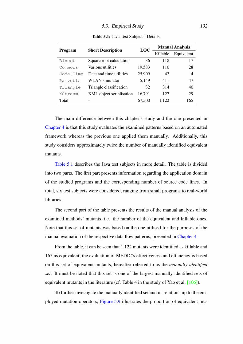
5.3. Empirical Study 132
Table 5.1: Java Test Subjects’ Details.
Program Short Description LOCManual Analysis
Killable Equivalent
Bisect Square root calculation 36 118 17Commons Various utilities 19,583 110 28Joda-Time Date and time utilities 25,909 42 4Pamvotis WLAN simulator 5,149 411 47Triangle Triangle classification 32 314 40XStream XML object serialisation 16,791 127 29Total - 67,500 1,122 165
The main difference between this chapter’s study and the one presented in
Chapter 4 is that this study evaluates the examined patterns based on an automated
framework whereas the previous one applied them manually. Additionally, this
study considers approximately twice the number of manually identified equivalent
mutants.
Table 5.1 describes the Java test subjects in more detail. The table is divided
into two parts. The first part presents information regarding the application domain
of the studied programs and the corresponding number of source code lines. In
total, six test subjects were considered, ranging from small programs to real-world
libraries.
The second part of the table presents the results of the manual analysis of the
examined methods’ mutants, i.e. the number of the equivalent and killable ones.
Note that this set of mutants was based on the one utilised for the purposes of the
manual evaluation of the respective data flow patterns, presented in Chapter 4.
From the table, it can be seen that 1,122 mutants were identified as killable and
165 as equivalent; the evaluation of MEDIC’s effectiveness and efficiency is based
on this set of equivalent mutants, hereafter referred to as the manually identified
set. It must be noted that this set is one of the largest manually identified sets of
equivalent mutants in the literature (cf. Table 4 in the study of Yao et al. [106]).
To further investigate the manually identified set and its relationship to the em-
ployed mutation operators, Figure 5.9 illustrates the proportion of equivalent mu-

5.3. Empirical Study 133
Arithmetic Operator Deletion Unary (1%)Conditional Operator Insertion (1%)Conditional Operator Replacement (2%)Logical Operator Insertion (4%)Arithmetic Operator Insertion Unary (5%)Arithmetic Operator Replacement Binary (7%)Relational Operator Replacement (19%)Arithmetic Operator Insertion Short-cut (61%)
Figure 5.9: Equivalent Mutants Per Mutation Operator. Contribution of each mutationoperator to the manually identified set of equivalent mutants.
tants per mutation operator (without including the ones that did not generate such
mutants). Recall that the employed mutation operators are all the method-level
operators of the MUJAVA framework. The depicted data suggest that the Arith-
metic Operator Insertion Short-cut (AOIS) and the Relational Operator Replace-
ment (ROR) mutation operators generated most of the studied equivalent mutants,
with AOIS generating more than 50% of them.
In order to measure MEDIC’s effectiveness, MEDIC was employed to the stud-
ied test subjects and the resulting set of automatically identified equivalent mutants
was compared to the manually identified one. Figure 5.10 presents this process. In
essence, the following steps were performed per test subject:
Step 1. WALA was applied to the classes that contained the manually identified
equivalent mutants of the corresponding subject.
Step 2. The output of WALA was automatically transformed into a format compat-
ible with MEDIC’s data model and then stored in a graph database.
Step 3. MEDIC utilised these data to detect the underlying equivalent and partially
equivalent mutants.
The first step of the aforementioned process entailed the application of the
WALA framework to randomly selected methods of the classes that were mutated

5.3. Empirical Study 134
ProgramunderTest WALA
PostAnalysis
Program Analysis
PartiallyEquivalentMutants
EquivalentMutants
Equivalent Mutant Identification
MEDIC
Neo4j
Figure 5.10: MEDIC’s Application Process. First, the program under test is analysedby WALA; second, WALA’s output is transformed into a format compatiblewith MEDIC’s data model and is stored in a NEO4J database; finally, MEDICutilises this model to identify the equivalent and partially equivalent mutantsof the examined program.
during the manual analysis phase. Next, the output of WALA was processed in
order to transform it into an appropriate format that was compatible with the data
model of MEDIC. This transformation was performed automatically by a script and
the adjusted output was stored in a NEO4J database. Finally, this database was given
as input to the MEDIC system in order to perform its analysis.
This process resulted in two sets of mutants: the set of automatically identified
equivalent mutants and the set of the partially equivalent ones. The former of these
sets is contrasted with the manually identified one in order to investigate MEDIC’s
effectiveness and the latter is utilised for the purposes of the RQ 5.3 research ques-
tion.
To study the efficiency of MEDIC, the run-time of the above-mentioned steps
was measured. The experiment was conducted on a physical machine running
GNU/Linux, equipped with an i7 processor (3,40 GHz, 4 cores) and 16GB of mem-
ory. Note that since the detection of partially equivalent mutants is integral to the
detection of equivalent ones, the corresponding findings refer to the time that both
these analyses required.

5.3. Empirical Study 135
Table 5.2: JavaScript Test Subjects’ Details.
Program Short Description LOCdojox.calendar Calendar widget 8,524D3 Visualisation library 11,594mathjs Mathematics library 13,112DateJS Date library 29,880Total - 63,110
5.3.2.2 RQ 5.2: Experimental Design
This research question examines whether MEDIC can detect equivalent and par-
tially equivalent mutants in programs implemented in different programming lan-
guages (apart from Java). To answer this question, MEDIC was also applied to a set
of test subjects written in JavaScript. This particular language was chosen because
WALA natively supports it and its application domain differs greatly from the one
of Java.
Table 5.2 presents details regarding the corresponding test subjects in a similar
fashion to the Java test subjects (cf. Table 5.1). As can be seen, a total of four test
subjects were considered, which vary in size and application domain; the latter of
these being the primary reason for their selection.
Owing to the fact that the studied research question is solely concerned with
the feasibility of detecting equivalent and partially equivalent mutants in different
programming languages, no exhaustive manual analysis of mutants was performed,
but rather the mutants that were identified by MEDIC as equivalent or partially
equivalent were manually inspected to ensure the correctness of the analysis.
The undertaken steps, for the purposes of this research question, are the same
as the steps of the first one with two exceptions. At the first step, WALA was
applied to randomly selected functions and, at the second step, the transformation
of WALA’s output was performed in a semi-automated fashion.
To elaborate on this, WALA’s support for the JavaScript programming lan-
guage did not cater for all the necessary information pertinent to MEDIC’s data
model. Specifically, it did not report the type of the examined variables. This fact
is not due to a limitation of the tool, but rather it is an inherent characteristic of the

5.3. Empirical Study 136
dynamic nature of JavaScript. To circumvent this issue, the corresponding informa-
tion was added manually, based on either available comments in the corresponding
source code or by inspecting the variables’ usage. The rest of WALA’s output was
transformed via an automated script.
5.3.2.3 RQ 5.3: Experimental Design
The final research question refers to the partially equivalent mutants and investigates
their killability. Recall that the examined set of partially equivalent mutants is the
one generated by MEDIC when applied to the Java test subjects.
The first step in addressing this question was to examine whether this set con-
sisted of killable or equivalent mutants based on the results of the manual analysis
(performed for the purposes of RQ 5.1). Next, the difficulty in killing these mutants
was investigated. To quantify such an intangible property the concept of stubborn
mutants [124] was utilised.
For the purposes of this study, a stubborn mutant is considered to be a killable
mutant that remains alive by a test suite that covers all the feasible branches of the
control flow graph of the program under test. The same definition was also adopted
in the study of Yao et al. [106]. Since a stubborn mutant cannot be killed by a branch
adequate test suite, it is considered harder to kill than a non-stubborn one. Thus,
if the partially equivalent mutant set consisted mainly of stubborn mutants then it
would contain hard-to-kill mutants, or, in the opposite situation, easy-to-kill ones.
The investigation of this research question is based on three metrics: (1) the
proportion of the partially equivalent mutants that are equivalent; (2) the proportion
of the partially equivalent mutants that are stubborn; and, (3) the proportion of the
stubborn mutants that are partially equivalent. In order to calculate these metrics,
the subsequent process was followed per test subject:
Step 1. The corresponding test subject was executed with the mutation adequate
test suite to discover the remaining uncovered branches.
Step 2. The discovered branches were manually inspected to determine their
(in)feasibility.

5.4. Empirical Findings 137
Step 3. The mutants of the test subject were executed against a set of five manually
constructed branch adequate test suites in order to determine the stubborn
ones.
Step 4. The stubborn partially equivalent mutants were discovered.
Step 5. The final results were averaged over the five repetitions.
The previously described process entails the identification of the branches of
the considered test subjects that were not covered by the mutation adequate test
suites and their manual inspection to determine their (in)feasibility. Note that the
mutation adequate test suites were created for the purposes of RQ 5.1.
Next, five branch adequate test suites were constructed in order to discover the
underlying stubborn mutants. These test suites were created in such a way that they
did not overlap each other. The reason for utilising five branch adequate test suites
instead of one is to cater for discrepancies caused by high quality test suites, i.e.
branch adequate test suites that kill more mutants than other analogous ones.
The next stage was to execute the mutants of each test subject with the previ-
ously constructed branch adequate test suites to determine the stubborn ones. The
stubborn mutants were the ones that remained alive and were not equivalent. Af-
ter the identification of the stubborn mutants, the stubborn partially equivalent ones
were determined. Finally, the aforementioned metrics were calculated based on all
five executions.
5.4 Empirical FindingsThis section details the empirical findings of the conducted experimental study. The
corresponding results are presented according to the relevant research question.
5.4.1 RQ 5.1: MEDIC’s Effectiveness and Efficiency
The first research question, RQ 5.1, investigates the effectiveness and efficiency
of MEDIC in detecting equivalent mutants. Table 5.3 presents the corresponding
findings with respect to the tool’s effectiveness.

5.4. Empirical Findings 138
Table 5.3: Automatically Identified Equivalent Mutants per Data Flow Pattern and JavaTest Subject. The middle part of the table presents the corresponding findingsgrouped by the relevant categories of the considered patterns.
ProgramCategories of Problematic Patterns
TotalUD DD UR DRSL SB DB SL SB DB SB DB
Bisect - 4 2 - 2 - - - - 8Commons - - 12 - - - 4 - - 16Joda-Time - - - - - - 4 - - 4Pamvotis - - - 11 - - 32 - - 43Triangle 4 - - - - - 14 - - 18XStream - - 4 - - - - - - 4Total 4 4 18 11 2 - 54 - - 93
The table is divided into three parts: the first part refers to the Java test sub-
jects; the middle part presents the automatically identified equivalent mutants per
data flow pattern; and the last one depicts the automatically identified equivalent
mutants per test subject. It should be mentioned that the results presented in the
middle part of the table are grouped by the corresponding categories of the studied
patterns. To exemplify, the UD column of the table refers to the Use-Def category
of patterns and its SL, SB and DB columns to the SameLine-UD, SameBB-UD and
DifferentBB-UD patterns, respectively. The results of the remaining patterns are
presented analogously.
By examining the table, it becomes obvious that MEDIC manages to automat-
ically identify 93 equivalent mutants for the Java test subjects, which corresponds
to a 56% reduction in the number of the examined equivalent mutants that have to
be manually analysed (cf. Table 5.1). Additionally, it can be seen that the UD and
UR categories of patterns identified the most equivalent mutants, followed by the
DD category of patterns.
Interestingly, three problematic patterns did not identify any equivalent mutant
for the Java test subjects. This fact does not limit their usefulness; the SameBB-
UR problematic pattern detected equivalent mutants of the JavaScript test subjects
and DifferentBB-DR identified partially equivalent ones belonging to the examined

5.4. Empirical Findings 139
0
20
40
60
80
100
AODU AOIS AOIU AORB COI COR LOI ROR
Nu
mbe
r of
Equ
ivale
nt M
uta
nts
Mutation Operators
Automatically identified
Figure 5.11: Automatically Identified Equivalent Mutants per Mutation Operator.The figure depicts the proportion of the automatically identified equivalentmutants per mutation operator for the Java test subjects.
Java programs. The only pattern that did not detect equivalent or partially equivalent
mutants for all test subjects is the SameBB-DR pattern.
In order to better investigate the nature of the automatically identified equiv-
alent mutants, Figure 5.11 visualises the proportion of these mutants (with respect
to all studied equivalent ones) per mutation operator. It is evident that the majority
of the equivalent mutants produced by the Arithmetic Operator Insertion Short-cut
(AOIS) and Arithmetic Operator Replacement Binary (AORB) mutation operators
were automatically identified. Recall that AOIS was the operator that produced the
most equivalent mutants (cf. Figure 5.9).
Additionally, equivalent mutants created by the Arithmetic Operator Insertion
Unary (AOIU) and Logical Operator Insertion (LOI) were also detected, although
in a smaller scale. It should be mentioned that all mutants detected by MEDIC as
equivalent were indeed equivalent ones and, thus, they can be weeded out safely.
The previous results lend colour to MEDIC’s effectiveness in detecting equiv-
alent mutants. Even though these findings are encouraging, the practicality of any

5.4. Empirical Findings 140
Table 5.4: Run-time of MEDIC’s Equivalent Mutant Detection Process for the Java TestSubjects (results are presented in seconds).
ProgramWALA Analysis MEDIC Analysis
Total(seconds)
Bisect 3 7 10Commons 5 7 12Joda-Time 4 3 7Pamvotis 10 18 28Triangle 3 15 18XStream 4 46 50Total 29 96 125
automated framework depends greatly on its efficiency. To provide insights regard-
ing the performance of MEDIC, Table 5.4 depicts the run-time of the corresponding
analysis. More precisely, it presents the run-time of the WALA framework when
applied to the examined test subjects and the respective one of the MEDIC system.
Note that all figures are in seconds.
It can be seen that MEDIC required approximately 96 seconds to complete
the equivalent mutant detection, utilising the program analysis data that had been
collected in 29 seconds. Recall that the program analysis was performed only for
the classes of the considered test subjects that contained the manually identified
equivalent mutants.
By examining the table, it becomes apparent that most of the studied classes
were analysed in under 30 seconds, with XStream’s one being the exception. The
increased run-time for the corresponding class is attributed to its internal complex-
ity and the large number of the available combinations of uses and definitions of
variables that MEDIC had to evaluate, which exceeded 150,000!
To summarise, MEDIC managed to automatically detect 93 equivalent mutants
in just 125 seconds. Assuming an equivalent mutant requires approximately 15
minutes of manual analysis [79], the analysis of the examined equivalent ones would
necessitate 165× 15 = 41 man-hours! The utilisation of MEDIC decreases this
cost from 41 to 18 man-hours, a 56% reduction in the manual effort involved, thus
boosting the practical adoption of mutation.

5.4. Empirical Findings 141
Table 5.5: Automatically Identified Equivalent Mutants per Data Flow Pattern andJavaScript Test Subject. The middle part of the table presents the correspondingfindings grouped by the relevant categories of the considered patterns.
ProgramCategories of Patterns
TotalUD DD URSL SB DB - SL SB DB
nthRoot 4 - - - - 4 4 12BisectJS - - 8 - 4 - - 12StorageManager - - - - - 2 2 4DateJS - - - - - - 2 2Total 4 - 8 - 4 6 8 30
Table 5.6: Automatically Identified Partially Equivalent Mutants per Data Flow Pattern andJavaScript Test Subject. The middle part of the table presents the correspondingfindings grouped by the relevant categories of the considered patterns.
ProgramData Flow Patterns
TotalDifferentBB-UD DD DifferentBB-UR
nthRoot - - 16 16BisectJS 4 - 8 12StorageManager - - 2 2DateJS - - - 0Total 4 - 26 30
5.4.2 RQ 5.2: Equivalent Mutant Detection in Different Pro-
gramming Languages
The results of this subsection are relevant to the cross-language nature of the
MEDIC framework, i.e. its capability to detect equivalent and partially equivalent
mutants in programs implemented in different programming languages. The corre-
sponding findings are depicted in Table 5.5 and Table 5.6. The former one presents
the automatically identified equivalent mutants and the latter, the partially equiv-
alent ones per studied data flow pattern and JavaScript test subject. Note that the
SameBB-DR and DifferentBB-DR patterns are not included in the tables because
they did not detect any such mutant.
From Table 5.5, which is structured in a similar fashion to Table 5.3, it can
be seen that 30 equivalent mutants were automatically identified, supporting the

5.4. Empirical Findings 142
Table 5.7: Partially Equivalent Mutants’ Killability. Proportion of equivalent and stubbornmutants w.r.t. the partially equivalent ones (column Part. Equivalent Mutants)and proportion of the stubborn partially equivalent mutants w.r.t. the total stub-born ones (column Stubborn Mutants).
ProgramPart. Equivalent Mutants Stubborn Mutants% Equivalent % Stubborn % Part. Equivalent
Bisect 5 4 11Commons 43 0 0Joda-Time 0 65 17Pamvotis 0 19 3Triangle 27 17 20XStream 0 4 5Grand Total 16 14 6
statement that MEDIC can detected equivalent mutants in different programming
languages. The findings of Table 5.6 lead to the same conclusion but in this case for
partially equivalent mutant detection.
The results of this subsection regarding the JavaScript test subjects and the
findings of the previous one regarding the examined Java programs provide clear
evidence to support the cross-language nature of the MEDIC framework. MEDIC
is the first tool that has been empirically evaluated to achieve such a task.
5.4.3 RQ 5.3: Partially Equivalent Mutants’ Killability
The final research question investigates the killability of the partially equivalent
mutants. Table 5.7 presents the corresponding findings. The table is divided into
two groups of columns: the first group presents the partially equivalent mutant set’s
proportion of equivalent and stubborn mutants; and the second one, the proportion
of the stubborn mutants that are partially equivalent ones.
It can be seen that 16% of the partially equivalent mutant set is composed
of equivalent mutants and 14% of stubborn ones, on average. Furthermore, these
stubborn mutants account for 6% of the total stubborn ones.
Figure 5.12 presents a Venn diagram illustrating the detected partially equiv-
alent mutant set (denoted as PE) and the corresponding killable (K), equivalent
(E) and stubborn (S) ones, in order to better visualise the relation between each of

5.4. Empirical Findings 143
All mutants
K S
PE E
Figure 5.12: Relation between PE and K, E and S Mutant Sets. The relation betweenthe Partially Equivalent (PE) mutant set and the corresponding Killable (K),Equivalent (E) and Stubborn (S) ones. (The size of the shapes is analogous tothe cardinality of the illustrated sets.)
them. From the depicted data, it becomes clear that the partially equivalent mutant
set contains equivalent and stubborn mutants, but consists largely of non-stubborn
ones, i.e. easy-to-kill ones.
Considering the above findings, one might decide to discard this set altogether.
Such a decision would result in a 12% additional reduction in the number of equiv-
alent mutants that have to be manually analysed and a 9% reduction in the number
of killable ones, for the studied test subjects. Although, such an act is not without
its perils, i.e. the removal of valuable mutants, the fact that only a small portion
of the killable mutants needs to be targeted in order to kill the whole generated set
seems to mitigate the underlying risk (see also Section 2.3.2.3).
To recapitulate this section’s findings, MEDIC managed to automatically de-
tect equivalent and partially equivalent mutants in the Java test subjects. MEDIC
identified 56% of the corresponding equivalent mutants in just 125 seconds. A re-
duction that can be further increased by 12% if the discovered partially equivalent
mutant set is discarded. These results indicate that MEDIC is a very cost-effective
tool, managing to detect a considerable number of equivalent mutants in a negligible
amount of time. Additionally, MEDIC identified equivalent and partially equivalent

5.4. Empirical Findings 144
mutants in the JavaScript test subjects. These findings support the cross-language
nature of the tool and suggest that the aforementioned benefits are not bound to a
specific programming language.
5.4.4 Threats to Validity
All empirical studies inevitably face specific limitations on the interpretation of their
results, this one is no exception. The present subsection discusses the corresponding
threats and presents the actions taken to ameliorate their effects. First, threats to
the construct validity are described and subsequently, the ones to the external and
internal validity are discussed.
• Threats to Construct Validity. This particular category is concerned with
the appropriateness of the measures utilised in the conducted experiments.
One threat that belongs to this category is relevant to the investigation of
the difficulty in killing the partially equivalent mutants. For the purposes of
this investigation, the proportion of the stubborn partially equivalent mutants
was utilised. Owing to the fact that a stubborn mutant is harder to kill than
a non-stubborn one, this metric is considered adequate for gaining insights
regarding the nature of the partially equivalent mutants.
• Threats to External Validity. This category of threats refers to the general-
isability of the obtained results. No empirical study can claim that its results
are generalisable in their entirety. Indeed, different studied programs or pro-
gramming languages could yield different results for any empirical study. To
mitigate these threats, the conducted empirical study was based on test sub-
jects of various size and application domain and a considerable number of
manually identified mutants. It should be mentioned that many of the studied
programs have also been utilised in previous research studies, e.g. [79, 145].
• Threats to Internal Validity. The threats to internal validity pertain to the
correctness of the conclusions of an empirical study. One such threat is rel-
evant to the manual analysis of the examined mutants and more precisely to
the detection of equivalent ones. To control this threat, a mutant was evalu-

5.5. Summary 145
ated thoroughly in order to be identified as equivalent. It should be mentioned
that this threat is a direct consequence of the undecidability of the equivalent
mutant problem and affects all the relevant mutation testing studies. Anal-
ogous considerations arise from the detection of stubborn mutants and, by
extension, the detection of stubborn partially equivalent ones. To mitigate
the effects of this threat, the corresponding process was based on five, non-
overlapping branch adequate test suites. A final threat to the internal validity
of the presented work is the correctness of the implementation of the WALA
and MEDIC frameworks. In order to cater for this threat, the results of both
tools were manually inspected to ascertain their correctness.
5.5 SummaryThis chapter introduced an automated, static analysis framework for equivalent and
partially equivalent mutant identification, named Mutants’ Equivalence Discovery
(MEDIC). MEDIC’s analysis is based on the problematic data flow patterns pro-
posed in the previous chapter whose presence in the source code of the program
under test leads to the generation of equivalent and partially equivalent mutants.
In order to investigate MEDIC’s effectiveness and efficiency, an empirical
study was conducted based on a manually analysed set of mutants from real-world
programs written in the Java programming language. In particular, this set consisted
of 1,122 killable mutants and 165 equivalent ones. The obtained results indicate that
MEDIC detected 56% of the considered equivalent mutants in just 125 seconds, a
run-time cost that is far from comparable to the corresponding manual effort which
approximates 23 man-hours (93 mutants × 15 minutes).
Apart from evaluating the detection power and performance of MEDIC, this
chapter was also concerned with the cross-language capabilities of the tool, i.e. it
was examined whether or not it could detect equivalent and partially equivalent
mutants in programs written in different programming languages. For this reason,
MEDIC was additionally applied to test subjects written in JavaScript. The respec-
tive findings suggest that MEDIC can indeed detect such mutants in the studied

5.5. Summary 146
JavaScript programs, indicating that the tool’s benefits are not confined to a specific
programming language.
The final research question that this chapter addresses pertains to the killability
of the partially equivalent mutants, i.e. whether or not they tend to be killable, and
the difficulty in performing such a task. To answer this question, (a) the proportion
of the partially equivalent mutants that are equivalent, (b) the proportion of the
partially equivalent mutants that are stubborn and (c) the proportion of the stubborn
mutants that are partially equivalent were calculated.
The obtained data indicate that 16% of the partially equivalent mutant set is
composed of equivalent mutants and 14% of stubborn ones, which account for 6%
of the total stubborn mutants. Thus, this set consists largely of non-stubborn mu-
tants, while containing equivalent ones. Based on these findings, one might decide
to discard the partially equivalent mutant set completely, realising a total reduction
of 68% in the number of the equivalent mutants that have to be manually analysed.
This translates into an additional 5 man-hour reduction in the involved manual ef-
fort, salvaging a total of 28 man-hours that would have been wasted otherwise.
Apart from the cross-language nature, the automated stubborn mutant detection
constitutes another unique feature of MEDIC.
Most of the previously introduced techniques for detecting equivalent mutants
require the generation, compilation and analysis of the corresponding mutants of
the program under test. In contrast, MEDIC is only applied to the original program.
Thus, it can be argued that MEDIC has a clear advantage over these techniques, as
far as efficiency is concerned.
The next chapter presents another approach to deal with the equivalent mutant
problem in the presence of software clones. To this end, the chapter introduces
the concept of mirrored mutants denoting mutants that belong to similar code frag-
ments of the examined program. It is postulated that such mutants exhibit similar
behaviour with respect to their equivalence and, thus, knowledge about the equiv-
alence of one of them could be utilised to classify others as possibly equivalent or
possibly killable ones. The conducted empirical investigation supports this intuition

5.5. Summary 147
and suggests that considerable effort savings can be achieved.
Chapter 6
Eliminating Equivalent Mutants via Code
Similarity
As mentioned in Chapter 2, mutation testing is a very powerful technique for testing
software, but is considered prohibitively expensive for practical adoption. This cost
is primarily attributed to the computational resources required for the execution
of the generated mutants and the human effort involved in finding appropriate test
cases to kill these mutants or determine their equivalence.
This chapter argues that knowledge about the already identified killable and
equivalent mutants can reduce mutation’s cost in the presence of software clones.
More precisely, given two similar code fragments, this work investigates whether
the killability or equivalence of the mutants of the one code fragment can determine
the killability or equivalence of the mutants of the other.
To this end, the concept of mirrored mutants is introduced, that is mutants that
belong to similar code fragments and, more precisely, to analogous code locations
within these fragments. The intuition behind this idea is that mirrored mutants
exhibit analogous behaviour with respect to their equivalence. If this argument
is true, then knowledge about the equivalence of one of them could be used to
determine the equivalence of the others. Thus, effort savings can be achieved by
manually analysing only one of the mirrored mutants and automatically inferring
the killability or equivalence of the others.
The contributions of the present chapter can be summarised in the following
points:

6.1. Background: Code Similarity 149
1. The introduction of the concept of mirrored mutants for alleviating the effects
of the equivalent mutant problem.
2. An empirical study, based on a set of approximately 800 manually analysed
mutants1 from several real-world programs, which provides evidence to sup-
port the usefulness of mirrored mutants at both the intra- and inter-method
level.
3. Experimental results pertaining to the utilisation of mirrored mutants for test
case generation purposes.
The rest of the chapter is organised as follows. Section 6.1 introduces the
necessary background information and Section 6.2 elaborates on the concept of
mirrored mutants. In Section 6.3, details about the conducted empirical study, the
experimental procedure, the obtained results and possible threats to their validity
are presented. Finally, Section 6.4 concludes this chapter.
6.1 Background: Code SimilarityThis section describes the necessary concepts with respect to code similarity, along
with examples from the conducted study.
Similar code fragments, which are termed code clones or software clones, exist
in software systems [169–171]. Their existence is attributed to the reuse of already
developed code, by means of copy and paste, with or without minor modifications.
The detection of these fragments is achieved by the employment of appropriate code
detection techniques [170, 171].
In clone detection terminology, a code fragment is any sequence of code lines,
with or without comments. A code clone of a code fragment c f 1 is another code
fragment, c f 2, which is similar to c f 1 by a given definition of similarity, i.e. given
a similarity function g, g(c f 1) = g(c f 2) [170]. The code fragments c f 1 and c f 2
form the clone pair (c f 1,c f 2). Note that code clones can appear at any level of
granularity (e.g. class level, method level, etc.).
1This set, along with the rest of the data of this chapter, is publicly available at: http://pages.cs.aueb.gr/˜kintism/#apsec2013

6.1. Background: Code Similarity 150
Clone detection techniques are based on two primary definitions of similarity
between code fragments, similarity based on program text and similarity based on
functionality [170]. In the former case, the syntactic similarity of their source code
is examined, whereas, in the latter, their semantic similarity is evaluated.
From the aforementioned definitions, different types of code clones are derived
(adapted from [170]):
• Type-1. Identical code fragments, except for variations in whitespace, layout
and comments.
• Type-2. Syntactically identical fragments, except for variations in identifiers,
literals, types, whitespace, layout and comments.
• Type-3. Copied fragments with further modifications such as changed, added
or removed statements, in addition to variations in identifiers, literals, types,
whitespace, layout and comments.
• Type-4. Two or more code fragments that perform the same computation, but
are implemented by different syntactic variants.
This chapter considers syntactic clones only, i.e. Type-1 to Type-3, and char-
acterises them as intra-method or inter-method according to whether or not they
belong to the same method. Type-4 code clones, although interesting, are left for
future research.
To denote a clone pair belonging to one file, the following notation is used:
([sl1 : sc1− el1 : ec1], [sl2 : sc2− el2 : ec2])
where sl1 and sc1 are the starting line and column of the first code fragment and el1
and ec1 the corresponding ending ones. Accordingly, sl2, sc2, el2 and ec2 refer to the
starting and ending lines and columns of the second code fragment. Note that in the
case of clone pairs that belong to different files, an identifier of the corresponding
files must be added to this notation.
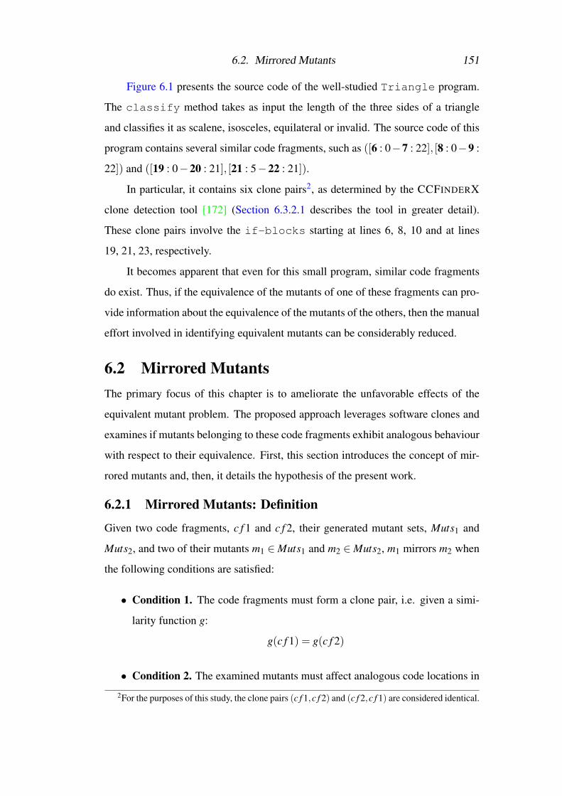
6.2. Mirrored Mutants 151
Figure 6.1 presents the source code of the well-studied Triangle program.
The classify method takes as input the length of the three sides of a triangle
and classifies it as scalene, isosceles, equilateral or invalid. The source code of this
program contains several similar code fragments, such as ([6 : 0−7 : 22], [8 : 0−9 :
22]) and ([19 : 0−20 : 21], [21 : 5−22 : 21]).
In particular, it contains six clone pairs2, as determined by the CCFINDERX
clone detection tool [172] (Section 6.3.2.1 describes the tool in greater detail).
These clone pairs involve the if-blocks starting at lines 6, 8, 10 and at lines
19, 21, 23, respectively.
It becomes apparent that even for this small program, similar code fragments
do exist. Thus, if the equivalence of the mutants of one of these fragments can pro-
vide information about the equivalence of the mutants of the others, then the manual
effort involved in identifying equivalent mutants can be considerably reduced.
6.2 Mirrored MutantsThe primary focus of this chapter is to ameliorate the unfavorable effects of the
equivalent mutant problem. The proposed approach leverages software clones and
examines if mutants belonging to these code fragments exhibit analogous behaviour
with respect to their equivalence. First, this section introduces the concept of mir-
rored mutants and, then, it details the hypothesis of the present work.
6.2.1 Mirrored Mutants: Definition
Given two code fragments, c f 1 and c f 2, their generated mutant sets, Muts1 and
Muts2, and two of their mutants m1 ∈Muts1 and m2 ∈Muts2, m1 mirrors m2 when
the following conditions are satisfied:
• Condition 1. The code fragments must form a clone pair, i.e. given a simi-
larity function g:
g(c f 1) = g(c f 2)
• Condition 2. The examined mutants must affect analogous code locations in
2For the purposes of this study, the clone pairs (c f 1,c f 2) and (c f 2,c f 1) are considered identical.

6.2. Mirrored Mutants 152
1: classify (int a, int b, int c) {2: int trian;3: if (a <= 0 || b <= 0 || c <= 0)4: return INVALID;5: trian = 0;6: if (a == b)7: trian = trian+1;8: if (a == c)9: trian = trian+2;
10: if (b == c)11: trian = trian+3;12: if (trian == 0)13: if (a + b < c || a + c < b || b + c < a)14: return INVALID;15: else16: return SCALENE;17: if (trian > 3)18: return EQUILATERAL;19: if (trian == 1 && a + b > c)20: return ISOSCELES;21: else if (trian == 2 && a + c > b)22: return ISOSCELES;23: else if (trian == 3 && b + c > a)24: return ISOSCELES;25: return INVALID;26: }
Figure 6.1: Source Code of the Triangle test subject.
these fragments, i.e. given l1 ∈ c f 1 and l2 ∈ c f 2 the lines that are affected by
m1 and m2, respectively, and linemap, a mapping3 between the lines of c f 1
and c f 2:
linemap(l1) = l2
• Condition 3. The mutants must induce analogous syntactic changes, i.e.
given op1 and op2 the mutation operators of m1 and m2, and a similarity
function f :
op1 = op2 ∧ f (l1) = f (l2)
Mutants m1 and m2 are termed mirrored mutants. According to whether or not
3Techniques to automatically generate such a mapping exist in the literature, cf. [173].

6.2. Mirrored Mutants 153
Mirrored Mutants Mutated Statement
AOIS 25 7: trian = trian ++ +1;
AOIS 37 9: trian = trian ++ +2;
AOIS 105 19: if (trian == 1 && a+b ++ > c)
AOIS 121 21: if (trian == 2 && a+ c ++ > b)
AORB 4 7: trian = trian − 1;
AORB 12 11: trian = trian − 3;
Figure 6.2: Examples of Mirrored Mutants from the Triangle test subject.
c f 1 and c f 2 belong to the same method, mirrored mutants can be characterised as
intra-method or inter-method ones.
Figure 6.2 presents three instances of mirrored mutants from the Triangle
test subject (presented in Figure 6.1). For each mutant, its name, the number of
the affected line, the induced change and the resulting statement are depicted. For
instance, the first pair, AOIS 25 and AOIS 37, which belongs to the ([6 : 0−
7 : 22], [8 : 0− 9 : 22]) clone pair4, is generated by inserting the post-increment
arithmetic operator (e.g. var++) at lines 7 and 9 of Figure 6.1, respectively.
Note that the mutation operator of the first pair of mirrored mutants, Arithmetic
Operator Insertion Short-cut (AOIS), generates three additional mutants per consid-
ered line at these specific code locations (++trian, −−trian and trian−−),
resulting in a total of four mutants per line. Although all these mutants affect the
same lines employing the same mutation operator, they form different mirrored mu-
tant sets.
By examining Figure 6.2 closely, it can be seen that the presented mutants af-
fect analogous code locations belonging to similar code lines of similar code frag-
ments, thus, they constitute mirrored mutants. It is argued that mirrored mutants
exhibit analogous behaviour with respect to their equivalence; the next subsection
discusses this hypothesis and presents a motivating example.
4The other mutants belong to: ([19 : 0− 20 : 21], [21 : 5− 22 : 21]) and ([6 : 0− 7 : 22], [10 :0−11 : 22]) clone pairs, respectively.

6.2. Mirrored Mutants 154
6.2.2 Mirrored Mutants and Equivalent Mutant Discovery
This work is based on the intuition that if a mutant mirrors other mutants and
has been identified as equivalent (or killable), then its mirrored ones could also
be equivalent (or killable). More formally, given two mirrored mutants, m1 and m2:
m1 ∈ equivs⇒ m2 ∈ equivs
where equivs is the set of equivalent mutants of the original program. Note that
although this statement does not constitute a mathematical theorem, its empirical
investigation suggests that it manages to provide substantial guidance in detecting
more equivalent mutants from the already identified ones (cf. Section 6.3.3).
Consider again Figure 6.2, the first two mirrored mutant pairs consist solely of
equivalent mutants (determined by manual analysis). In the first case, the value of
variable trian is used unmodified, then it is incremented by one (due to the post-
increment operator) and finally, it is redefined by the evaluation of the whole state-
ment. Thus, the induced change can never be detected. Although, the equivalent
mutants of the first pair can be considered trivial, i.e. they are relatively easy to
identify, the ones of the second pair require a more thorough examination and a
better understanding of the internal mechanics of the program.
In both cases, the effort involved in manually analysing the examined mutants
could be considerably reduced by leveraging the previously described property; in-
stead of manually analysing four mutants, the analysis could be restricted to two
mutants that mirror the others, e.g. AOIS 25 and AOIS 105, and thus the equiv-
alence of the mirrored ones, i.e. AOIS 37 and AOIS 121, could be automatically
determined.
This statement also holds true in the case of automated equivalent mutant iden-
tification. For example, since AOIS 25 can be automatically detected as equivalent
by the SameLine-UD data flow pattern, described in Section 4.2.2.1, in the presence
of mirrored mutants, the automated detection of one of these mutants suffices.
The last mirrored mutant pair of Figure 6.2 demonstrates the opposite situation.
It can be easily seen that AORB 4 and AORB 12 can be killed, thus, knowledge

6.3. Empirical Study and Results 155
about the non-equivalence of the one of them could be used to determine the non-
equivalence of the other. In this study, experimental results suggesting that mirrored
mutants can be beneficial to test case generation processes are also provided.
More precisely, it is postulated that a test case that kills a mutant can be trans-
formed into an appropriate one that kills its mirrored ones. For instance, the test
case (a = 2, b = 2, c = 1) that kills AORB 4 can be appropriately transformed to
kill AORB 12 based on information derived from the corresponding clone pair. By
examining the ([6 : 0−7 : 22], [10 : 0−11 : 22]) clone pair, it becomes evident that
variable a is replaced with b and b with c, thus, a similar transformation at the test
case level could produce a test case able to kill AORB 12. Indeed, the resulting test
case (a= 1, b= 2, c= 2) manages to kill the corresponding mutant. Although find-
ing such an automatic transformation technique is out of the scope of this work, it is
presented as another interesting aspect of mirrored mutants and a possible direction
for future research.
To summarise, mirrored mutants contribute to the elimination of equivalent
mutants and potentially to test case generation processes that target these particular
mutants. The next section furnishes a detailed view of the experimental study, along
with the research questions that are being investigated.
6.3 Empirical Study and ResultsThe present study examines whether mirrored mutants can be of assistance in dis-
covering more equivalent mutants from the already identified ones. To this end, an
experimental study based on a set of manually analysed mirrored mutants was con-
ducted. This section describes the underlying experimental procedure, the obtained
results and the actions taken to mitigate possible threats to validity.
6.3.1 Research Questions
The research questions that are investigated by this study are the following:
• RQ 6.1 Do mirrored mutants exhibit analogous behaviour with respect to
their equivalence?

6.3. Empirical Study and Results 156
• RQ 6.2 In the case of killable mutants, can mirrored mutants contribute to
the test case generation process?
Although the above research objectives are sound, an additional point should
be investigated: Do mirrored mutants appear in adequate numbers in real-world
programs?
This is an important question because if mirrored mutants appear scarcely in
software systems, then their underlying benefits would be negligible. In a different
case, significant effort savings could be achieved. By definition, mirrored mutants
are closely related to the number of similar code fragments in the program under
test. Thus, the above question can be restated as: To what extent do real world
programs contain duplicated code?, or equally, Does a considerable number of
clone pairs exist in software systems?
Fortunately, this question has already been answered in the literature of clone
detection. In particular, studies suggest that the percentage of cloned code of a
typical software system lies between 7% and 23% [169, 174]. Considering that
applying mutation testing to a program of 30 lines could produce over 300 mutants,
then its application to even the 7% of the lines of a large software system would
produce a considerable number of mirrored mutants.
6.3.2 Experimental Study
6.3.2.1 Supporting Tools
For the purposes of this study, the CCFINDERX clone detection tool [172, 175]
(version 10.2.7.4) and the MUJAVA mutation testing framework [19, 163] (version
3) were utilised. A brief description of these tools follows:
• Clone Detection. CCFINDERX is a state-of-the-art token-based clone de-
tection tool and constitutes a major upgrade of CCFINDER [175]. The
tool supports various programming languages, e.g. Java, C, COBOL, etc.,
and has been applied to large software systems [175]. Several experimen-
tal studies have evaluated its ability to detect software clones, e.g. [170],
and concluded that it manages to successfully detect all types of syntactic

6.3. Empirical Study and Results 157
clones. In this study, CCFINDERX was employed to detect similar code frag-
ments in the considered test subjects with the minimumclonelength and
minimumTKS options set to 10.
• Mutant Generation. The MUJAVA testing framework is a tool for applying
mutation testing to programs implemented in the Java programming language.
It supports method-level and class-level mutation operators. The method-
level operators target the unit level and were designed based on the selective
mutation approach [81] (see also Table 4.1), whereas the class-level operators
target specific object-oriented features. The MUJAVA tool is a rather mature
framework that has been utilised by many research studies, e.g. [87, 176].
In this study, the considered mutants were generated by applying all method-
level mutation operators of the tool.
6.3.2.2 Test Subjects
This empirical study was conducted on a set of six test subjects (written in Java),
most of which have been utilised in previous research studies, e.g. [78]. Table 6.1
presents details about the corresponding programs.
The first four columns of the table outline the id of the test subjects that
uniquely identifies them and will be used in subsequent tables, e.g. Table 6.3, their
name, a brief description of their usage and the corresponding source code lines5.
The last column presents the number of the corresponding clone sets, as determined
by CCFINDERX. Note that a clone set contains one or more clone pairs.
It should be mentioned that some minor modifications to Pamvotis were
performed in order to enable the application of the MUJAVA framework. This was
necessary due to specific limitations of the tool, e.g. it cannot handle programs util-
ising the generics feature of Java. These modifications did not affect the semantics
of the program.
5Generated by SLOCCOUNT (http://www.dwheeler.com/sloccount/).

6.3. Empirical Study and Results 158
Table 6.1: Test Subjects’ Details.
Id Program Description LOC Clone Sets1 Bisect Square root calculation 36 12 Commons Various utilities 19,583 1,1263 Joda-Time Date and time utilities 25,909 1,6784 Pamvotis WLAN simulator 5,149 4685 Triangle Triangle classification 32 36 Xstream XML object serialisation 16,791 710- Total - 67,500 3,986
6.3.2.3 Experimental Design
The experimental procedure of this study necessitated two steps; the discovery of a
random sample of mirrored mutants and its corresponding manual analysis. These
steps allowed the investigation of whether or not mirrored mutants share common
characteristics with respect to their equivalence.
The process of finding a random sample of mirrored mutants is illustrated in
Figure 6.3. For each test subject, the CCFINDERX tool was employed to detect
all possible similar code fragments. Next, a clone pair was chosen at random and
its mutants were generated by MUJAVA. If their number was greater than 40, the
corresponding mirrored mutants were discovered by mapping the mutants of the
one code fragment onto the ones of the other. Recall that a clone pair comprises
two similar code fragments. This restriction on the number of mutants was imposed
in order to prohibit the selection of clone pairs that produced very few mutants. The
aforementioned process was repeated, until a suitable match was found.
Table 6.2 presents information on the obtained mirrored mutant pairs. Column
“Rand. CPs” refers to the number of the randomly selected clone pairs per test
subject, column “MMPs” to the number of the respective mirrored mutant pairs,
column “Mutants” to the number of mutants that were manually analysed and col-
umn “Test Cases” to the number of test cases that were generated during the manual
analysis process. It should be mentioned that these test cases do not form a mini-
mum test set that is able to kill the corresponding mutants.
As can be seen from the table, the previously described procedure yielded 409
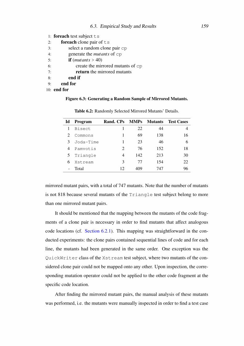
6.3. Empirical Study and Results 159
1: foreach test subject ts2: foreach clone pair of ts3: select a random clone pair cp4: generate the mutants of cp5: if (mutants > 40)6: create the mirrored mutants of cp7: return the mirrored mutants8: end if9: end for
10: end for
Figure 6.3: Generating a Random Sample of Mirrored Mutants.
Table 6.2: Randomly Selected Mirrored Mutants’ Details.
Id Program Rand. CPs MMPs Mutants Test Cases1 Bisect 1 22 44 42 Commons 1 69 138 163 Joda-Time 1 23 46 64 Pamvotis 2 76 152 185 Triangle 4 142 213 306 Xstream 3 77 154 22- Total 12 409 747 96
mirrored mutant pairs, with a total of 747 mutants. Note that the number of mutants
is not 818 because several mutants of the Triangle test subject belong to more
than one mirrored mutant pairs.
It should be mentioned that the mapping between the mutants of the code frag-
ments of a clone pair is necessary in order to find mutants that affect analogous
code locations (cf. Section 6.2.1). This mapping was straightforward in the con-
ducted experiments: the clone pairs contained sequential lines of code and for each
line, the mutants had been generated in the same order. One exception was the
QuickWriter class of the Xstream test subject, where two mutants of the con-
sidered clone pair could not be mapped onto any other. Upon inspection, the corre-
sponding mutation operator could not be applied to the other code fragment at the
specific code location.
After finding the mirrored mutant pairs, the manual analysis of these mutants
was performed, i.e. the mutants were manually inspected in order to find a test case

6.3. Empirical Study and Results 160
Table 6.3: Manual Analysis of Mirrored Mutants.
Gran. Class(es) Killable Equiv.
Method1:Bisect 40 45:Triangle 183 306:XmlFriendlyNameCoder 72 8
Class2:WordUtils 110 286:QuickWriter 74 0
I-Class3:Minutes,Seconds 42 44:Simulator,SourceManager 142 10
Total - 663 84
able to kill them. If such a test case could be found, the mutant was identified as
killable. In the opposite situation, it was classified as equivalent.
The results are presented in Table 6.3. The corresponding mirrored mutants are
divided into three categories according to the granularity level of their respective
clone pairs: the ”Method” and ”Class” categories, which refer to the intra-method
and intra-class levels and the ”I-Class” category, which denotes the inter-class level.
In the first category, mirrored mutants belong to the same method, in the second,
to different methods of the same class, and in the last one, to different methods of
different classes.
The first column of the table presents the aforementioned categories, the sub-
sequent ones, the id of the corresponding test subject, along with the name of the
considered class (or classes in the case of I-Class) and the number of killable and
equivalent mirrored mutants. In summary, 747 mirrored mutants were manually
analysed, 663 of which were determined killable and 84 equivalent.
In order to answer RQ 6.1, i.e. whether mirrored mutants can be of benefit
when dealing with the equivalent mutant problem, the following procedure was
undertaken: For each mirrored mutant pair (m1,m2), m2 was classified as equivalent
(or killable) based on the result of the manual analysis for m1. Note that the results
of the manual analysis were used only for one of the mutants of the considered
mirrored mutant pair. The remaining one was classified accordingly, heuristically
(cf. Section 6.2.2).

6.3. Empirical Study and Results 161
Afterwards, these classification results were evaluated against those of the
manual analysis and the ratio of the correctly classified equivalent (or killable) mir-
rored mutant pairs to the total number of classified mirrored mutant pairs of the
specific category was calculated. This metric is widely used in the area of Informa-
tion Retrieval [156] and is termed precision. The formal definition of this metric is
given in Equation 3.1.
Precision has been utilised in several, previous studies, evaluating different
mutant classification techniques, e.g. [78, 79]. A high precision score indicates that
the classification outcome of a mutant will most likely be the same as the one of the
respective manual analysis. A low one indicates the opposite situation.
It should be mentioned that in the cases of Bisect, Triangle and
XmlFriendlyNameCoder, some mutants could be differently classified based
on the order the corresponding mutants of the respective mirrored mutant pairs were
examined, i.e. some mirrored mutant pairs contained both killable and equivalent
mutants and, thus, the classification process would lead to different results accord-
ing to which mutant’s manually analysed results will be used. In these cases, the
classification process was employed to both mutants of the corresponding pairs and
the average precision was calculated.
The precision metric is usually complemented by the recall value, which mea-
sures the retrieval capability of a classifier [156]. In this study, the recall metric
was not utilised based on two reasons. First, the examined approach is not a clas-
sifier; the examined property of mirrored mutants necessitates previous knowledge
of the equivalence of the underlying mirrored mutants. Second, in this particular
case, the precision and the recall values are closely intertwined in such a way that
a high precision corresponds to a high recall score. To elaborate, in the case of
equivalent mutants for instance, if mirrored mutants exhibit the sought behaviour in
their equivalence, then the mutants classified as equivalent will be equivalent, lead-
ing to a high precision score, but, at the same time, most equivalent mutants will
also be retrieved, leading to a high recall score (see also Equation 3.2 for the formal
definition of this metric).

6.3. Empirical Study and Results 162
In order to investigate RQ 6.2, i.e. whether mirrored mutants can contribute
to test case generation processes that target them, the subsequent steps were fol-
lowed: for each mirrored mutant pair (m1,m2) in which m1 was determined killable
by manual analysis, the transformation of the corresponding test case that killed
m1 based on information derived from the respective clone pair was attempted (an
example demonstrating such a transformation was given in Section 6.2.2). If a
transformation was found, then the ability of the resulting test case to kill m2 was
examined. Thus, the employed metric is the ratio of the number of mirrored mu-
tant pairs for which such a transformation was possible to the number of all killable
mirrored mutant pairs.
6.3.3 Experimental Results
The obtained experimental results are depicted in Table 6.4 and Table 6.5. The
former details the obtained results pertaining to RQ 6.1 and RQ 6.2 and the latter,
an estimation of the cost reduction achieved by the presence of mirrored mutants.
Table 6.4 is divided into two parts. The first part (column “Precision”) presents
the precision metric with respect to both killable and equivalent mirrored mutants.
Note that, for QuickWriter, the precision metric was not calculated in the case
of equivalent mirrored mutants because all of its mutants were killable.
It can be seen that mirrored mutants can be leveraged to discover equivalent
and killable mutants based on the already identified ones. Specifically, in the case of
killable mirrored mutants at the intra-method level, an average precision of 98% is
realised, whereas at the intra- and inter-class levels a precision of 100% is achieved,
indicating that the results of the classification process are tantamount to the ones of
the manual analysis.
In the case of equivalent mirrored mutants, the corresponding results are 88%,
100% and 100%, respectively, suggesting a reasonable equivalent mutant classifica-
tion process. At this point, it should be mentioned that none of the examined clone
pairs was of Type-1, i.e. the corresponding code fragments were not identical (cf.
Section 6.1). Thus, the results cannot be attributed to the examination of identical
source code.

6.3. Empirical Study and Results 163
Table 6.4: Mirrored Mutants: Experimental Results.
Class(es)Precision Test Data
Killable Equivalents Transformation1:Bisect 100% 100% 60%5:Triangle 97% 84% 89%6:XmlFriendlyNameCoder 97% 80% 89%Average (Method) 98% 88% 79%
2:WordUtils 100% 100% 100%6:QuickWriter 100% - 100%Average (Class) 100% 100% 100%
3:Minutes,Seconds 100% 100% 100%4:Simulator,SourceManager 100% 100% 100%Average (I-Class) 100% 100% 100%
The second part of Table 6.4 (column “Test Data Transformation”) presents
results regarding RQ 6.2, i.e. whether or not a test case that kills a mutant of a mir-
rored mutant pair can be transformed to kill the other mutant(s) of the corresponding
pair, based on information derived from the respective clone pair.
The obtained data suggest that this transformation is feasible and the resulting
test cases are indeed able to kill the respective mutants. At the intra-method level,
79% of the total number of killable mirrored mutant pairs could produce such a
test case, on average. For the remaining categories, this transformation was always
possible (i.e. 100% in all cases).
To better understand the cost reduction achieved by leveraging mirrored mu-
tants, Table 6.5 presents the ratio of equivalent mutants that are automatically clas-
sified as such to the total number of equivalent mutants. More precisely, the table
depicts the number of equivalent mutants per considered class, the number of the
manually analysed ones, the number of the automatically determined ones and the
corresponding cost reduction measure.
It can be seen that approximately 50% of the total equivalent mutants of the
considered test subjects can be automatically classified as such. Note that the num-
ber of the automatically determined equivalent mutants of the Triangle test sub-
ject is greater than the one of the manually analysed equivalent mutants due to the

6.3. Empirical Study and Results 164
Table 6.5: Mirrored Mutants: Cost Reduction w.r.t. Manual Analysis of Equivalent Mu-tants.
Class(es)CR Analysis
Cost ReductionEquiv. Man. Auto.
1:Bisect 4 2 2 50%5:Triangle 30 10 17 56%6:XmlFriendlyNameCoder 8 4 3 38%Average (Method) - - - 48%
2:WordUtils 28 14 14 50%6:QuickWriter - - - -Average (Class) - - - 50%
3:Minutes,Seconds 4 2 2 50%4:Simulator,SourceManager 10 5 5 50%Average (I-Class) - - - 50%
fact that several equivalent mutants belong to more than one mirrored mutant pairs.
Conclusively, from the presented results, it can be argued that mirrored mutants
can be beneficial to the equivalent mutant identification process by reducing the
number of equivalent mutants that have to be manually analysed. In addition, they
can be potentially valuable to test case generation processes by providing a way to
transform the already available killing test cases into appropriate ones that can kill
other mirrored mutants.
6.3.4 Threats to Validity
Every research study has limitations concerning the interpretation of its results and
is exposed to possible threats related to its validity. This subsection discusses the
underlying threats and presents the actions taken to mitigate their effects.
• Threats to External Validity. This category refers to threats that affect the
generalisation of the obtained results. To weaken these threats, the con-
ducted experiments were based on approximately 800 manually identified
mirrored mutants, belonging to several open source projects of various size
and complexity that have been previously used in similar research studies, e.g.
[78, 79]. Additionally, results based on small test subjects, e.g. Triangle
and Bisect, were only reported at the intra-method level. At this particular

6.4. Summary 165
granularity level, the size of the examined program should not be of impor-
tance. Although no study can claim that its results are widely generalisable,
the examined property of mirrored mutants is believed to be independent of
the studied projects and more related to the similar structure of cloned code.
• Threats to Internal Validity. Concerning potential threats pertaining to the
internal validity, i.e. the ability to draw conclusions based on the studied
factors, the manual classification of the mirrored mutants was an area that
necessitated appropriate actions. More precisely, the manual identification
of the equivalent mutants, due to the difficulty of the underlying problem, is
subject to errors. To circumvent this problem, the mutants that were manually
categorised as equivalent were examined thoroughly. Furthermore, all the
results of this study are publicly available to support wider scrutiny.
6.4 SummaryThis chapter presented another approach to ameliorate the adverse effects of the
equivalent mutant problem in the presence of software clones. To this end, the
concept of mirrored mutants is introduced.
Mirrored mutants are mutants that belong to similar code fragments of the
program under test. It is posited that mirrored mutants exhibit analogous behaviour
with respect to their equivalence and, thus, in the presence of such mutants, the
manual cost of identifying equivalent mutants can be substantially reduced.
The chapter investigated whether or not mirrored mutants exhibit the afore-
mentioned behaviour and whether they can be of assistance to test case generation
processes. In order to answer the posed research questions, an empirical study
based on approximately 800 manually analysed mirrored mutants belonging to sev-
eral open source projects and different granularity levels was conducted.
The results of the study provide evidence supporting the aforementioned state-
ment. More precisely, the obtained findings suggest that approximately 50% of
studied equivalent mutants that belong to mirrored mutant pairs can be automati-
cally classified as such. Additionally, the study presented experimental results indi-

6.4. Summary 166
cating that test cases that kill a mutant of a mirrored mutant pair can be transformed
into appropriate test cases that kill the remaining mirrored mutants of the corre-
sponding pair.
It should be mentioned that the equivalent mutant detection techniques intro-
duced in the previous chapters of this thesis, or in the literature of Mutation Testing
in general, are orthogonal to the technique presented in this chapter. To elaborate,
these approaches can be applied first to detect equivalent mutants that belong to
mirrored mutant pairs and, next, the remaining mirrored mutants can be automati-
cally classified as equivalent ones. Thus, the manual cost of identifying equivalent
mutants could be further decreased.

Chapter 7
Conclusions and Future Work
Mutation testing is one of the most effective techniques in testing software. Unfor-
tunately, its adoption in practice is hindered by its cost. One of the main sources of
mutation’s cost is the manual effort involved in the detection of equivalent mutants
and, more precisely, the Equivalent Mutant Problem.
The Equivalent Mutant Problem is a well-known impediment to the adoption of
mutation testing in practice. Its undecidable nature renders a complete automated
solution unattainable. This situation is exacerbated further by the complexity of
the underlying manual analysis and the large number of mutants that have to be
considered. As a direct consequence, automated frameworks that can tackle this
issue are scarce.
This thesis introduces several novel techniques that can automatically elimi-
nate equivalent mutants, thus, reducing mutation’s manual cost and improving its
practical adoption. The dissertation’s contributions can be summarised in the fol-
lowing points:
• A Novel Mutant Classification Technique (Chapter 3)
This thesis proposed a novel mutant classification technique, named Higher
Order Mutation (HOM) classifier, that utilises second order mutants to auto-
matically classify first order ones. Additionally, the thesis introduced a new
mutant classification scheme, named Isolating Equivalent Mutants (I-EQM)
classifier, that combines effectively the state-of-the-art Coverage Impact clas-
sifier with the HOM classifier. The conducted experimental study that com-

168
pared the effectiveness of the aforementioned classifiers, based on real-world
test subjects, showed that I-EQM, with a precision score of 71% and a re-
call value of 81%, outperforms the examined approaches. The obtained re-
sults suggest that I-EQM manages to correctly classify approximately 20%
more killable mutants with only a 2% loss on its precision, leading to a more
thorough testing process. These findings are also supported by the accuracy
metric and Fβ scores of the classifier and by the conducted statistical analy-
sis of the obtained results. Finally, the relationship between mutants’ impact
and mutants’ killability was also investigated. The obtained findings indicate
that mutants with the highest impact do not necessarily guarantee the highest
killability ratios.
• Data Flow Patterns for Equivalent Mutant Detection (Chapter 4)
Nine data flow patterns that can detect equivalent and partially equivalent mu-
tants were introduced and formally defined in the present thesis. A partially
equivalent mutant is a mutant that is equivalent to the program under test for
a specific subset of paths. The main characteristic of their definition is that it
is based on the Static Single Assignment (SSA) intermediate representation
of the program under test. In essence, these patterns model specific problem-
atic situations between variable definitions and uses whose existence in the
program’s source code will lead to the generation of equivalent mutants. An
empirical study based on approximately 800 manually analysed mutants from
real-world test subjects was conducted to examine the patterns’ existence in
real-world programs and their equivalent mutant detection power. The ob-
tained results revealed that these patterns are indeed present in real-world
software and that they can automatically detect approximately 70% of the
studied equivalent mutants, thus, paving the way for the efficient application
of mutation testing.
• A Static Analysis Framework for Equivalent Mutant Detection (Chap-
ter 5)

169
The thesis introduced MEDIC (Mutants’ Equivalence Discovery), a static
analysis tool, written in the Jython programming language, that implements
the aforementioned patterns and manages to automatically detect equivalent
and partially equivalent mutants in different programming languages. To in-
vestigate MEDIC’s effectiveness and efficiency, an empirical study based on
approximately 1,300 manually analysed mutants from several real-world pro-
grams, written in the Java programming language, was conducted. The re-
spective results indicate that MEDIC manages to detect 56% of the studied
equivalent mutants in 125 seconds, providing strong evidence of the tool’s ef-
fectiveness and efficiency. Additionally, MEDIC successfully detected such
mutants in test subjects written in JavaScript, lending colour to the tool’s
cross-language nature. MEDIC’s ability to detect equivalent mutants in dif-
ferent programming languages is a unique characteristic of the tool. Finally,
the killability of the detected partially equivalent mutants was also examined.
The respective findings reveal that 14% of these mutants are stubborn ones,
suggesting that MEDIC can also detect automatically stubborn mutants.
• Laveraging Software Clones to Eliminate Equivalent Mutants (Chap-
ter 6)
This thesis introduced the concept of mirrored mutants, that is mutants be-
longing to similar code fragments and, particularly, to analogous code loca-
tions within these fragments. It is argued that mirrored mutants exhibit anal-
ogous behaviour with respect to their equivalence and that knowledge about
the equivalence of one of them can be used to determine the equivalence of
the others, thus, reducing the manual overhead of mutation. This assumption
was empirically investigated based on 747 manually analysed mutants from
real-world programs. The obtained results demonstrate that mirrored mutants
can considerably reduce mutation’s manual cost in the presence of software
clones. Additionally, experimental results suggesting that test cases that kill
mirrored mutants can be automatically transformed into appropriate ones that
kill other mirrored mutants, with a success rate higher than 80%, were also

170
presented.
Based on the aforementioned contributions, several future research directions
can be pursued. Most notably:
Elimination of Higher Order Equivalent Mutants. One possible future
research direction is the investigation of appropriate techniques to eliminate
higher order equivalent mutants. Although higher order equivalent mutants
are not as common as first order equivalent ones, such approaches could
be beneficial to higher order mutation approximation strategies (cf. Sec-
tion 2.3.1.1). Towards this direction, the mutant classification techniques pre-
sented in Chapter 3 seem to be a natural choice: since the HOM and I-EQM
classifiers manage to isolate first order equivalent mutants based on second
order ones, it would be interesting to explore whether this practice could be
generalised, i.e. whether it is possible to isolate n order equivalent mutants
via (n+1) order mutants.
Mutation Approximation Techniques based on HOM and I-EQM Classi-
fiers. Another potential research direction is the investigation of the effective-
ness of mutation approximation techniques that are based on the HOM and
I-EQM classifiers. Mutation approximation strategies based on the Coverage
Impact classifier have been evaluated in the literature of mutation testing and
have been found less effective than mutation (cf. Section 2.3.1.3). It would
be interesting to explore whether the utilisation of the HOM and I-EQM clas-
sifiers will make a difference.
Complementing MEDIC’s Equivalent Mutant Detection Process.
MEDIC’s empirical evaluation provides strong evidence of the tool’s effi-
ciency. Thus, an apparent future direction is the investigation of synergistic
ways in which MEDIC can be combined with other equivalent mutant de-
tection approaches. Based on the findings of the conducted experimental
study, a prominent direction is the combination of MEDIC with techniques
that can target equivalent mutants affecting branch predicates, since such
171
equivalent mutants comprised approximately 20% of the generated ones (cf.
Section 5.3.2.1). Due to MEDIC’s efficiency, the analysis of the resulting
equivalent mutant detection technique will not be hampered by the utilisation
of more than one tools.
MEDIC and Different Programming Languages. Another avenue for fur-
ther research is the application of MEDIC to additional programming lan-
guages. MEDIC has already been successfully applied to the Java and
JavaScript programming languages. It would also be interesting to examine
MEDIC’s performance when applied to programs written in other program-
ming languages. Although this will entail the utilisation of different program
analysis frameworks, MEDIC relies on a language-agnostic data model that
facilitates this task.
Generalising the Concept of Mirrored Mutants. Mirrored mutants have
been shown to reduce mutation’s cost in the presence of software clones. One
particularly interesting research direction is the investigation of whether this
concept can reduce the cost of other coverage criteria. For example, in the
case of the branch coverage criterion, it would be interesting to investigate
whether branches that belong to similar code fragments exhibit analogous
behaviour with respect to their infeasibility, i.e. whether mirrored branches
exist. If this is true for several coverage criteria, then the concept of mirrored
mutants can be generalised to the concept of mirrored test requirements.
Mirrored Mutants and Different Programming Languages. Another pos-
sible research direction is the evaluation of the concept of mirrored mutants
in other programming languages (apart from Java). Such languages could
employ different mutation operators that affect the source code of the pro-
gram under test in different ways. Thus, it would be useful to study whether
mirrored mutants are beneficial to the reduction of mutation’s manual cost in
different programming languages.

Appendix A
Publications
A.1 Refereed Journal Papers• M. Kintis and N. Malevris, “MEDIC: A static analysis framework for equiv-
alent mutant identification,” Information and Software Technology (IST),
vol. 68, pp. 1 – 17, 2015
• M. Kintis, M. Papadakis, and N. Malevris, “Employing second-order muta-
tion for isolating first-order equivalent mutants,” Software Testing, Verifica-
tion and Reliability (STVR), Special Issue on Mutation Testing, vol. 25, no.
5-7, pp. 508–535, 2015
A.2 Refereed Conference and Workshop Papers• M. Kintis and N. Malevris, “Using data flow patterns for equivalent mutant
detection,” in Proceedings of the 7th International Conference on Software
Testing, Verification and Validation Workshops (ICSTW), March 2014, pp.
196–205
• M. Kintis and N. Malevris, “Identifying more equivalent mutants via code
similarity,” in Proceedings of the 20th Asia-Pacific Software Engineering
Conference (APSEC), 2013, vol. 1, December 2013, pp. 180–188
• M. Kintis, M. Papadakis, and N. Malevris, “Isolating first order equiva-
lent mutants via second order mutation,” in Proceedings of the 5th Interna-

A.2. Refereed Conference and Workshop Papers 173
tional Conference on Software Testing, Verification and Validation Workshops
(ICSTW), April 2012, pp. 701–710
• M. Kintis, M. Papadakis, and N. Malevris, “Evaluating mutation testing al-
ternatives: A collateral experiment,” in Proceedings of the 17th Asia-Pacific
Software Engineering Conference (APSEC), 2010, November 2010, pp. 300–
309
• M. Papadakis, N. Malevris, and M. Kintis, “Mutation testing strategies - A
collateral approach,” in Proceedings of the 5th International Conference on
Software and Data Technologies (ICSOFT), Volume 2, July 2010, pp. 325–
328

Bibliography
[1] G. Myers, The Art of Software Testing. New York: John Wiley & Sons,
1979.
[2] I. Sommerville, Software Engineering, 6th ed. New York: Addison Wesley,
2001.
[3] P. Ammann and J. Offutt, Introduction to Software Testing, 1st ed. New
York, NY, USA: Cambridge University Press, 2008.
[4] R. Lipton, “Fault diagnosis of computer programs,” Student Report, Carnegie
Mellon University, 1971.
[5] R. A. DeMillo, “Test adequacy and program mutation,” in Proceedings of
the 11th International Conference on Software Engineering, ser. ICSE ’89.
New York, NY, USA: ACM, 1989, pp. 355–356.
[6] M. R. Woodward, “Mutation testing-an evolving technique,” in Software
Testing for Critical Systems, IEE Colloquium on, Jun 1990, pp. 3/1–3/6.
[7] M. Woodward, “Mutation testing — its origin and evolution,” Information
and Software Technology, vol. 35, no. 3, pp. 163 – 169, 1993.
[8] A. J. Offutt and R. H. Untch, “Mutation 2000: Uniting the orthogonal,” in
Mutation Testing for the New Century, ser. The Springer International Se-
ries on Advances in Database Systems, W. Wong, Ed. Springer US, 2001,
vol. 24, pp. 34–44.

BIBLIOGRAPHY 175
[9] Y. Jia and M. Harman, “An analysis and survey of the development of mu-
tation testing,” Software Engineering, IEEE Transactions on, vol. 37, no. 5,
pp. 649–678, 2011.
[10] A. P. Mathur, Foundations of Software Testing. Pearson Education, 2008.
[11] T. A. Budd and F. G. Sayward, “Users guide to the Pilot mutation system.”
Department of Computer Science, Yale University, Tech. Rep. 114, 1977.
[12] A. T. Acree, T. A. Budd, R. A. DeMillo, R. J. Lipton, and F. G. Sayward,
“Mutation analysis.” School of Information and Computer Science, Georgia
Institute of Technology, Tech. Rep. GIT-ICS-79/08, September 1979.
[13] K. N. King and A. J. Offutt, “A Fortran language system for mutation-based
software testing,” Software: Practice and Experience, vol. 21, no. 7, pp.
685–718, Jun. 1991.
[14] H. Agrawal, R. Demillo, R. Hathaway, W. Hsu, W. Hsu, E. Krauser, R. J.
Martin, A. Mathur, and E. Spafford, “Design of mutant operators for the C
programming language,” Technical Report SERC-TR-41-P, Software Engi-
neering Research Center, Purdue University, Tech. Rep., 1989.
[15] J. Maldonado, M. Delamaro, S. Fabbri, A. Silva Simao, T. Sugeta, A. Vin-
cenzi, and P. Masiero, “Proteum: A family of tools to support specification
and program testing based on mutation,” in Mutation Testing for the New
Century, ser. The Springer International Series on Advances in Database Sys-
tems, W. Wong, Ed. Springer US, 2001, vol. 24, pp. 113–116.
[16] Y. Jia and M. Harman, “Milu: A customizable, runtime-optimized higher
order mutation testing tool for the full C language,” in Practice and Research
Techniques, 2008. TAIC PART ’08. Testing: Academic Industrial Conference,
Aug 2008, pp. 94–98.
[17] S. Kim, J. Clark, and J. McDermid, “Investigating the effectiveness of object-
oriented strategies with the mutation method,” in Mutation Testing for the

BIBLIOGRAPHY 176
New Century, ser. The Springer International Series on Advances in Database
Systems, W. Wong, Ed. Springer US, 2001, vol. 24, pp. 4–4.
[18] P. Chevalley, “Applying mutation analysis for object-oriented programs using
a reflective approach,” in Software Engineering Conference, 2001. APSEC
2001. Eighth Asia-Pacific, Dec 2001, pp. 267–270.
[19] Y.-S. Ma, J. Offutt, and Y. R. Kwon, “MuJava: an automated class mutation
system,” Software Testing, Verification and Reliability, vol. 15, no. 2, pp.
97–133, 2005.
[20] D. Schuler and A. Zeller, “Javalanche: Efficient mutation testing for Java,”
in Proceedings of the the 7th Joint Meeting of the European Software Engi-
neering Conference and the ACM SIGSOFT Symposium on The Foundations
of Software Engineering, ser. ESEC/FSE ’09. New York, NY, USA: ACM,
2009, pp. 297–298.
[21] R. Just, “The Major mutation framework: Efficient and scalable mutation
analysis for Java,” in Proceedings of the 2014 International Symposium on
Software Testing and Analysis, ser. ISSTA 2014. New York, NY, USA:
ACM, 2014, pp. 433–436.
[22] L. Madeyski and N. Radyk, “Judy – a mutation testing tool for Java,” IET
Software, vol. 4, pp. 32–42, February 2010.
[23] M. Gligoric, S. Badame, and R. Johnson, “SMutant: A tool for type-sensitive
mutation testing in a dynamic language,” in Proceedings of the 19th ACM
SIGSOFT Symposium and the 13th European Conference on Foundations of
Software Engineering, ser. ESEC/FSE ’11. New York, NY, USA: ACM,
2011, pp. 424–427.
[24] A. Derezinska and K. Hałas, “Experimental evaluation of mutation testing
approaches to python programs,” in Software Testing, Verification and Val-
idation Workshops (ICSTW), 2014 IEEE Seventh International Conference
on, March 2014, pp. 156–164.

BIBLIOGRAPHY 177
[25] D. Le, M. A. Alipour, R. Gopinath, and A. Groce, “MuCheck: An extensible
tool for mutation testing of Haskell programs,” in Proceedings of the 2014
International Symposium on Software Testing and Analysis, ser. ISSTA 2014.
New York, NY, USA: ACM, 2014, pp. 429–432.
[26] S. Mirshokraie, A. Mesbah, and K. Pattabiraman, “Efficient javascript mu-
tation testing,” in Software Testing, Verification and Validation (ICST), 2013
IEEE Sixth International Conference on, March 2013, pp. 74–83.
[27] S. Mirshokraie, A. Mesbah, and K. Pattabiraman, “Guided mutation testing
for JavaScript web applications,” Software Engineering, IEEE Transactions
on, vol. 41, no. 5, pp. 429–444, May 2015.
[28] W. Chan, S. Cheung, and T. Tse, “Fault-based testing of database application
programs with conceptual data model,” in Quality Software, 2005. (QSIC
2005). Fifth International Conference on, Sept 2005, pp. 187–196.
[29] J. Tuya, M. Suarez-Cabal, and C. De La Riva, “SQLMutation: A tool to gen-
erate mutants of sql database queries,” in Mutation Analysis, 2006. Second
Workshop on, Nov 2006, pp. 1–1.
[30] J. Tuya, M. J. Surez-Cabal, and C. de la Riva, “Mutating database queries,”
Information and Software Technology, vol. 49, no. 4, pp. 398 – 417, 2007.
[31] C. Zhou and P. Frankl, “Mutation testing for java database applications,” in
Software Testing Verification and Validation, 2009. ICST ’09. International
Conference on, April 2009, pp. 396–405.
[32] C. Zhou and P. Frankl, “JDAMA: Java database application mutation anal-
yser,” Software Testing, Verification and Reliability, vol. 21, no. 3, pp. 241–
263, 2011.
[33] T. A. Budd and A. S. Gopal, “Program testing by specification mutation,”
Computer Languages, vol. 10, no. 1, pp. 63 – 73, 1985.

BIBLIOGRAPHY 178
[34] R. A. DeMillo, R. J. Lipton, and F. G. Sayward, “Hints on test data selection:
Help for the practicing programmer,” Computer, vol. 11, no. 4, pp. 34–41,
1978.
[35] M. Delamaro, J. Maldonado, and A. Mathur, “Integration testing using in-
terface mutation,” in Software Reliability Engineering, 1996. Proceedings.,
Seventh International Symposium on, Oct 1996, pp. 112–121.
[36] P. Mateo, M. Usaola, and J. Offutt, “Mutation at system and functional lev-
els,” in Software Testing, Verification, and Validation Workshops (ICSTW),
2010 Third International Conference on, April 2010, pp. 110–119.
[37] P. R. Mateo, M. P. Usaola, and J. Offutt, “Mutation at the multi-class and
system levels,” Science of Computer Programming, vol. 78, no. 4, pp. 364 –
387, 2013, special section on Mutation Testing and Analysis (Mutation 2010)
&; Special section on the Programming Languages track at the 25th {ACM}
Symposium on Applied Computing.
[38] S. Pinto Ferraz Fabbri, M. Delamaro, J. Maldonado, and P. Masiero, “Mu-
tation analysis testing for finite state machines,” in Software Reliability En-
gineering, 1994. Proceedings., 5th International Symposium on, Nov 1994,
pp. 220–229.
[39] R. Hierons and M. Merayo, “Mutation testing from probabilistic finite state
machines,” in Testing: Academic and Industrial Conference Practice and Re-
search Techniques - MUTATION, 2007. TAICPART-MUTATION 2007, Sept
2007, pp. 141–150.
[40] C. Jing, Z. Wang, X. Shi, X. Yin, and J. Wu, “Mutation testing of protocol
messages based on extended TTCN-3,” in Advanced Information Network-
ing and Applications, 2008. AINA 2008. 22nd International Conference on,
March 2008, pp. 667–674.
[41] T. Mouelhi, Y. Le Traon, and B. Baudry, “Mutation analysis for security
tests qualification,” in Testing: Academic and Industrial Conference Practice

BIBLIOGRAPHY 179
and Research Techniques - MUTATION, 2007. TAICPART-MUTATION 2007,
Sept 2007, pp. 233–242.
[42] E. Martin and T. Xie, “A fault model and mutation testing of access control
policies,” in Proceedings of the 16th International Conference on World Wide
Web, ser. WWW ’07. New York, NY, USA: ACM, 2007, pp. 667–676.
[43] Y. Le Traon, T. Mouelhi, and B. Baudry, “Testing security policies: Going
beyond functional testing,” in Software Reliability, 2007. ISSRE ’07. The 18th
IEEE International Symposium on, Nov 2007, pp. 93–102.
[44] C. Henard, M. Papadakis, G. Perrouin, J. Klein, and Y. Le Traon, “Assess-
ing software product line testing via model-based mutation: An application
to similarity testing,” in Software Testing, Verification and Validation Work-
shops (ICSTW), 2013 IEEE Sixth International Conference on, March 2013,
pp. 188–197.
[45] C. Henard, M. Papadakis, and Y. Le Traon, “Mutation-based generation of
software product line test configurations,” in Search-Based Software Engi-
neering, ser. Lecture Notes in Computer Science, C. Le Goues and S. Yoo,
Eds. Springer International Publishing, 2014, vol. 8636, pp. 92–106.
[46] C. Wright, G. Kapfhammer, and P. McMinn, “Efficient mutation analysis
of relational database structure using mutant schemata and parallelisation,”
in Software Testing, Verification and Validation Workshops (ICSTW), 2013
IEEE Sixth International Conference on, March 2013, pp. 63–72.
[47] C. Wright, G. Kapfhammer, and P. McMinn, “The impact of equivalent, re-
dundant and quasi mutants on database schema mutation analysis,” in Qual-
ity Software (QSIC), 2014 14th International Conference on, Oct 2014, pp.
57–66.
[48] R. DeMillo and A. Offutt, “Constraint-based automatic test data generation,”
Software Engineering, IEEE Transactions on, vol. 17, no. 9, pp. 900–910,
Sep 1991.

BIBLIOGRAPHY 180
[49] R. A. DeMillo and A. J. Offutt, “Experimental results from an automatic test
case generator,” ACM Transactions on Software Engineering and Methodol-
ogy, vol. 2, no. 2, pp. 109–127, Apr. 1993.
[50] Y. Le Traon, B. Baudry, and J. Jezequel, “Design by contract to improve
software vigilance,” Software Engineering, IEEE Transactions on, vol. 32,
no. 8, pp. 571–586, Aug 2006.
[51] M. Papadakis and N. Malevris, “Automatic mutation test case generation via
dynamic symbolic execution,” in Software Reliability Engineering (ISSRE),
2010 IEEE 21st International Symposium on, Nov 2010, pp. 121–130.
[52] L. Zhang, T. Xie, L. Zhang, N. Tillmann, J. de Halleux, and H. Mei, “Test
generation via dynamic symbolic execution for mutation testing,” in Software
Maintenance (ICSM), 2010 IEEE International Conference on, Sept 2010,
pp. 1–10.
[53] M. Papadakis and N. Malevris, “Mutation based test case generation via a
path selection strategy,” Information and Software Technology, vol. 54, no. 9,
pp. 915 – 932, 2012.
[54] G. Fraser and A. Zeller, “Mutation-driven generation of unit tests and ora-
cles,” Software Engineering, IEEE Transactions on, vol. 38, no. 2, pp. 278–
292, 2012.
[55] T. Xie, N. Tillmann, J. de Halleux, and W. Schulte, “Mutation analysis of
parameterized unit tests,” in Software Testing, Verification and Validation
Workshops, 2009. ICSTW ’09. International Conference on, April 2009, pp.
177–181.
[56] A. J. Offutt, J. Pan, and J. M. Voas, “Procedures for reducing the size of
coverage-based test sets,” in In Proceedings of the Twelfth International Con-
ference on Testing Computer Software, 1995, pp. 111–123.

BIBLIOGRAPHY 181
[57] L. Zhang, D. Marinov, L. Zhang, and S. Khurshid, “Regression mutation
testing,” in Proceedings of the 2012 International Symposium on Software
Testing and Analysis, ser. ISSTA 2012. New York, NY, USA: ACM, 2012,
pp. 331–341.
[58] M. Papadakis and Y. Le Traon, “Using mutants to locate ”unknown” faults,”
in Software Testing, Verification and Validation (ICST), 2012 IEEE Fifth In-
ternational Conference on, April 2012, pp. 691–700.
[59] S. Moon, Y. Kim, M. Kim, and S. Yoo, “Ask the mutants: Mutating faulty
programs for fault localization,” in Software Testing, Verification and Valida-
tion (ICST), 2014 IEEE Seventh International Conference on, March 2014,
pp. 153–162.
[60] M. Papadakis and Y. Le Traon, “Metallaxis-fl: mutation-based fault local-
ization,” Software Testing, Verification and Reliability, vol. 25, no. 5-7, pp.
605–628, 2015.
[61] E. Alegroth, Z. Gao, R. Oliveira, and A. Memon, “Conceptualization and
evaluation of component-based testing unified with visual gui testing: An
empirical study,” in Software Testing, Verification and Validation (ICST),
2015 IEEE 8th International Conference on, April 2015, pp. 1–10.
[62] R. Oliveira, E. Alegroth, Z. Gao, and A. Memon, “Definition and evaluation
of mutation operators for gui-level mutation analysis,” in Software Testing,
Verification and Validation Workshops (ICSTW), 2015 IEEE Eighth Interna-
tional Conference on, April 2015, pp. 1–10.
[63] R. Geist, A. Offutt, and J. Harris, F.C., “Estimation and enhancement of
real-time software reliability through mutation analysis,” Computers, IEEE
Transactions on, vol. 41, no. 5, pp. 550–558, May 1992.
[64] M. Daran and P. Thevenod-Fosse, “Software error analysis: A real case study
involving real faults and mutations,” in Proceedings of the 1996 ACM SIG-

BIBLIOGRAPHY 182
SOFT International Symposium on Software Testing and Analysis, ser. ISSTA
’96. New York, NY, USA: ACM, 1996, pp. 158–171.
[65] J. H. Andrews, L. C. Briand, and Y. Labiche, “Is mutation an appropriate tool
for testing experiments?” in Proceedings of the 27th International Confer-
ence on Software Engineering, ser. ICSE ’05. New York, NY, USA: ACM,
2005, pp. 402–411.
[66] J. Andrews, L. Briand, Y. Labiche, and A. Namin, “Using mutation analysis
for assessing and comparing testing coverage criteria,” Software Engineer-
ing, IEEE Transactions on, vol. 32, no. 8, pp. 608–624, Aug 2006.
[67] H. Do and G. Rothermel, “On the use of mutation faults in empirical assess-
ments of test case prioritization techniques,” Software Engineering, IEEE
Transactions on, vol. 32, no. 9, pp. 733–752, Sept 2006.
[68] R. Just, D. Jalali, L. Inozemtseva, M. D. Ernst, R. Holmes, and G. Fraser,
“Are mutants a valid substitute for real faults in software testing?” in Pro-
ceedings of the 22Nd ACM SIGSOFT International Symposium on Founda-
tions of Software Engineering, ser. FSE 2014. New York, NY, USA: ACM,
2014, pp. 654–665.
[69] A. J. Offutt and J. M. Voas, “Subsumption of condition coverage techniques
by mutation testing,” Department of Information and Software Systems En-
gineering, George Mason University, Tech. Rep. ISSE-TR-96-100, 1996.
[70] N. Li, U. Praphamontripong, and J. Offutt, “An experimental comparison of
four unit test criteria: Mutation, edge-pair, all-uses and prime path coverage,”
in Software Testing, Verification and Validation Workshops, 2009. ICSTW
’09. International Conference on, April 2009, pp. 220–229.
[71] A. J. Offutt, J. Pan, K. Tewary, and T. Zhang, “Experiments with data flow
and mutation testing.” Department of Information and Software Systems En-
gineering, George Mason University, Tech. Rep. ISSE-TR-94-105, 1994.
BIBLIOGRAPHY 183
[72] A. P. Mathur and W. E. Wong, “An empirical comparison of data flow and
mutation-based test adequacy criteria,” Software Testing, Verification and Re-
liability, vol. 4, no. 1, pp. 9–31, 1994.
[73] A. J. Offutt, J. Pan, K. Tewary, and T. Zhang, “An experimental evaluation of
data flow and mutation testing,” Software: Practice and Experience, vol. 26,
no. 2, pp. 165–176, 1996.
[74] P. G. Frankl, S. N. Weiss, and C. Hu, “All-uses vs mutation testing: An
experimental comparison of effectiveness,” Journal of Systems and Software,
vol. 38, no. 3, pp. 235 – 253, 1997.
[75] S. Rapps and E. J. Weyuker, “Data flow analysis techniques for test data
selection,” in Proceedings of the 6th International Conference on Software
Engineering, ser. ICSE ’82. Los Alamitos, CA, USA: IEEE Computer
Society Press, 1982, pp. 272–278.
[76] S. Rapps and E. J. Weyuker, “Selecting software test data using data flow
information,” IEEE Transactions on Software Engineering, vol. SE-11, no. 4,
pp. 367–375, April 1985.
[77] P. G. Frankl and E. J. Weyuker, “An applicable family of data flow testing
criteria,” IEEE Transactions on Software Engineering, vol. 14, no. 10, pp.
1483–1498, Oct 1988.
[78] D. Schuler and A. Zeller, “(Un-)Covering equivalent mutants,” in Software
Testing, Verification and Validation (ICST), 2010 Third International Con-
ference on, April 2010, pp. 45–54.
[79] D. Schuler and A. Zeller, “Covering and uncovering equivalent mutants,”
Software Testing, Verification and Reliability, vol. 23, no. 5, pp. 353–374,
2013.
[80] L. Madeyski, W. Orzeszyna, R. Torkar, and M. Jozala, “Overcoming the
equivalent mutant problem: A systematic literature review and a comparative

BIBLIOGRAPHY 184
experiment of second order mutation,” Software Engineering, IEEE Transac-
tions on, vol. 40, no. 1, pp. 23–42, Jan 2014.
[81] A. J. Offutt, A. Lee, G. Rothermel, R. H. Untch, and C. Zapf, “An experi-
mental determination of sufficient mutant operators,” ACM Transactions on
Software Engineering and Methodology, vol. 5, no. 2, pp. 99–118, Apr. 1996.
[82] W. E. Howden, “Completeness criteria for testing elementary program func-
tions,” in Proceedings of the 5th International Conference on Software En-
gineering, ser. ICSE ’81. Piscataway, NJ, USA: IEEE Press, 1981, pp.
235–243.
[83] W. E. Howden, “Weak mutation testing and completeness of test sets,” IEEE
Trans. Softw. Eng., vol. 8, no. 4, pp. 371–379, Jul. 1982.
[84] M. Woodward and K. Halewood, “From weak to strong, dead or alive? an
analysis of some mutation testing issues,” in Software Testing, Verification,
and Analysis, 1988., Proceedings of the Second Workshop on, Jul 1988, pp.
152–158.
[85] M. Polo, M. Piattini, and I. Garca-Rodrguez, “Decreasing the cost of muta-
tion testing with second-order mutants,” Software Testing, Verification and
Reliability, vol. 19, no. 2, pp. 111–131, 2009.
[86] Y. Jia and M. Harman, “Higher order mutation testing,” Information and
Software Technology, vol. 51, no. 10, pp. 1379 – 1393, 2009, Source Code
Analysis and Manipulation, {SCAM} 2008.
[87] M. Kintis, M. Papadakis, and N. Malevris, “Evaluating mutation testing al-
ternatives: A collateral experiment,” in Proceedings of the 17th Asia-Pacific
Software Engineering Conference (APSEC), 2010, November 2010, pp. 300–
309.
[88] M. Papadakis and N. Malevris, “An empirical evaluation of the first and
second order mutation testing strategies,” in Software Testing, Verification,

BIBLIOGRAPHY 185
and Validation Workshops (ICSTW), 2010 Third International Conference
on, April 2010, pp. 90–99.
[89] T. Budd and D. Angluin, “Two notions of correctness and their relation to
testing,” Acta Informatica, vol. 18, no. 1, pp. 31–45, 1982.
[90] R. G. Hamlet, “Testing programs with the aid of a compiler,” Software Engi-
neering, IEEE Transactions on, vol. SE-3, no. 4, pp. 279–290, 1977.
[91] R. A. DeMillo, D. S. Guindi, W. M. McCracken, A. J. Offutt, and K. N.
King, “An extended overview of the Mothra software testing environment,”
in Software Testing, Verification, and Analysis, 1988., Proceedings of the
Second Workshop on, Jul 1988, pp. 142–151.
[92] T. A. Budd, R. A. DeMillo, R. J. Lipton, and F. G. Sayward, “Theoretical and
empirical studies on using program mutation to test the functional correctness
of programs,” in Proceedings of the 7th ACM SIGPLAN-SIGACT Symposium
on Principles of Programming Languages, ser. POPL ’80. New York, NY,
USA: ACM, 1980, pp. 220–233.
[93] A. Offutt, “The coupling effect: Fact or fiction,” in Proceedings of the ACM
SIGSOFT ’89 Third Symposium on Software Testing, Analysis, and Verifica-
tion, ser. TAV3. New York, NY, USA: ACM, 1989, pp. 131–140.
[94] A. J. Offutt, “Investigations of the software testing coupling effect,” ACM
Transactions on Software Engineering and Methodology, vol. 1, no. 1, pp.
5–20, Jan. 1992.
[95] R. J. Lipton and F. G. Sayward, “The status of research on program muta-
tion,” in the Workshop on Software Testing and Test Documentation, 1978,
pp. 355–373.
[96] L. J. Morell, “A theory of error-based testing,” Ph.D. dissertation, University
of Maryland, 1984.

BIBLIOGRAPHY 186
[97] K. S. H. T. Wah, “Fault coupling in finite bijective functions,” Software Test-
ing, Verification and Reliability, vol. 5, no. 1, pp. 3–47, 1995.
[98] K. S. H. T. Wah, “A theoretical study of fault coupling,” Software Testing,
Verification and Reliability, vol. 10, no. 1, pp. 3–45, 2000.
[99] K. Kapoor, “Formal analysis of coupling hypothesis for logical faults,” Inno-
vations in Systems and Software Engineering, vol. 2, no. 2, pp. 80–87, 2006.
[100] T. A. Budd, “Mutation analysis of program test data,” Ph.D. dissertation, Yale
University, 1980.
[101] E. Barr, M. Harman, P. McMinn, M. Shahbaz, and S. Yoo, “The oracle prob-
lem in software testing: A survey,” Software Engineering, IEEE Transactions
on, vol. 41, no. 5, pp. 507–525, May 2015.
[102] A. T. Acree, “On mutation,” Ph.D. dissertation, Georgia Institute of Technol-
ogy, 1980.
[103] L. Morell, “A theory of fault-based testing,” Software Engineering, IEEE
Transactions on, vol. 16, no. 8, pp. 844–857, Aug 1990.
[104] J. Offutt, “Automatic test data generation,” Ph.D. dissertation, Georgia Insti-
tute of Technology, 1988.
[105] J. M. Voas and G. McGraw, Software Fault Injection: Inoculating Programs
Against Errors. New York, NY, USA: John Wiley & Sons, 1997.
[106] X. Yao, M. Harman, and Y. Jia, “A study of equivalent and stubborn mutation
operators using human analysis of equivalence,” in Proceedings of the 36th
International Conference on Software Engineering, ser. ICSE 2014. New
York, NY, USA: ACM, 2014, pp. 919–930.
[107] M. Kintis, “Mutation testing and its approximations,” Master’s thesis, De-
partment of Informatics, Athens University of Economics and Business,
2010, (in greek).

BIBLIOGRAPHY 187
[108] H. Agrawal, “Dominators, super blocks, and program coverage,” in Proceed-
ings of the 21st ACM SIGPLAN-SIGACT Symposium on Principles of Pro-
gramming Languages, ser. POPL ’94. New York, NY, USA: ACM, 1994,
pp. 25–34.
[109] M. Papadakis, N. Malevris, and M. Kintis, “Mutation testing strategies - A
collateral approach,” in Proceedings of the 5th International Conference on
Software and Data Technologies (ICSOFT), Volume 2, July 2010, pp. 325–
328.
[110] K. Adamopoulos, M. Harman, and R. Hierons, “How to overcome the
equivalent mutant problem and achieve tailored selective mutation using co-
evolution,” in Genetic and Evolutionary Computation GECCO 2004, ser.
Lecture Notes in Computer Science, K. Deb, Ed. Springer Berlin Heidel-
berg, 2004, vol. 3103, pp. 1338–1349.
[111] D. Baldwin and F. Sayward, “Heuristics for determining equivalence of pro-
gram mutations.” Department of Computer Science, Yale University, Tech.
Rep. 276, 1979.
[112] A. J. Offutt and W. M. Craft, “Using compiler optimization techniques to de-
tect equivalent mutants,” Software Testing, Verification and Reliability, vol. 4,
no. 3, pp. 131–154, 1994.
[113] M. Papadakis, Y. Jia, M. Harman, and Y. Le Traon, “Trivial compiler equiva-
lence: A large scale empirical study of a simple, fast and effective equivalent
mutant detection technique,” in Proceedings of the 2015 International Con-
ference on Software Engineering, 2015, to appear.
[114] A. J. Offutt and J. Pan, “Automatically detecting equivalent mutants and in-
feasible paths,” Software Testing, Verification and Reliability, vol. 7, no. 3,
pp. 165–192, 1997.
[115] A. J. Offutt and J. Pan, “Detecting equivalent mutants and the feasible path
problem,” in Computer Assurance, 1996. COMPASS ’96, Systems Integrity.

BIBLIOGRAPHY 188
Software Safety. Process Security. Proceedings of the Eleventh Annual Con-
ference on, Jun 1996, pp. 224–236.
[116] S. Nica and F. Wotawa, “Using constraints for equivalent mutant detection,”
in Formal Methods in the Development of Software, 2012. WS-FMDS 2012.,
Proceedings of the Second Workshop on, 2012, pp. 1–8.
[117] S. Nica and F. Wotawa, “EqMutDetect – A tool for equivalent mutant de-
tection in embedded systems,” in Intelligent Solutions in Embedded Systems,
2012. WISES 2012., Proceedings of the Tenth Workshop on, 2012, pp. 57–62.
[118] S. Bardin, M. Delahaye, R. David, N. Kosmatov, M. Papadakis, Y. L. Traon,
and J. Y. Marion, “Sound and quasi-complete detection of infeasible test re-
quirements,” in Software Testing, Verification and Validation (ICST), 2015
IEEE 8th International Conference on, April 2015, pp. 1–10.
[119] N. Malevris, “A path generation method for testing LCSAJs that restrains
infeasible paths,” Information and Software Technology, vol. 37, no. 8, pp.
435 – 441, 1995.
[120] M. N. Ngo and H. B. K. Tan, “Heuristics-based infeasible path detection for
dynamic test data generation,” Information and Software Technology, vol. 50,
no. 7-8, pp. 641 – 655, 2008.
[121] M. Papadakis and N. Malevris, “A symbolic execution tool based on the
elimination of infeasible paths,” in Software Engineering Advances (ICSEA),
2010 Fifth International Conference on, Aug 2010, pp. 435–440.
[122] M. Weiser, “Program slicing,” in Proceedings of the 5th International Con-
ference on Software Engineering, ser. ICSE ’81. Piscataway, NJ, USA:
IEEE Press, 1981, pp. 439–449.
[123] J. M. Voas and G. McGraw, Software Fault Injection: Inoculating Programs
Against Errors. New York, NY, USA: John Wiley & Sons, Inc., 1997.

BIBLIOGRAPHY 189
[124] R. Hierons, M. Harman, and S. Danicic, “Using program slicing to assist
in the detection of equivalent mutants,” Software Testing, Verification and
Reliability, vol. 9, no. 4, pp. 233–262, 1999.
[125] D. Binkley, “Computing amorphous program slices using dependence
graphs,” in Proceedings of the 1999 ACM Symposium on Applied Computing,
ser. SAC ’99. New York, NY, USA: ACM, 1999, pp. 519–525.
[126] M. Harman and S. Danicic, “Amorphous program slicing,” in Program Com-
prehension, 1997. IWPC ’97. Proceedings., Fifth Iternational Workshop on,
Mar 1997, pp. 70–79.
[127] M. Harman, R. Hierons, and S. Danicic, “The relationship between program
dependence and mutation analysis,” in Mutation Testing for the New Cen-
tury, ser. The Springer International Series on Advances in Database Sys-
tems, W. Wong, Ed. Springer US, 2001, vol. 24, pp. 5–13.
[128] M. Ellims, D. Ince, and M. Petre, “The Csaw C mutation tool: Initial results,”
in Testing: Academic and Industrial Conference Practice and Research Tech-
niques - MUTATION, 2007. TAICPART-MUTATION 2007, Sept 2007, pp.
185–192.
[129] B. Grun, D. Schuler, and A. Zeller, “The impact of equivalent mutants,” in
Software Testing, Verification and Validation Workshops, 2009. ICSTW ’09.
International Conference on, April 2009, pp. 192–199.
[130] D. Schuler, V. Dallmeier, and A. Zeller, “Efficient mutation testing by check-
ing invariant violations,” in Proceedings of the Eighteenth International Sym-
posium on Software Testing and Analysis, ser. ISSTA ’09. New York, NY,
USA: ACM, 2009, pp. 69–80.
[131] M. Papadakis and Y. Le Traon, “Mutation testing strategies using mutant
classification,” in Proceedings of the 28th Annual ACM Symposium on Ap-
plied Computing, ser. SAC ’13. New York, NY, USA: ACM, 2013, pp.
1223–1229.

BIBLIOGRAPHY 190
[132] M. Papadakis, M. Delamaro, and Y. Le Traon, “Mitigating the effects of
equivalent mutants with mutant classification strategies,” Science of Com-
puter Programming, vol. 95, Part 3, pp. 298 – 319, 2014.
[133] W. E. Wong, “On mutation and data flow,” Ph.D. dissertation, Purdue Uni-
versity, 1993.
[134] A. J. Offutt, G. Rothermel, and C. Zapf, “An experimental evaluation of se-
lective mutation,” in Proceedings of the 15th International Conference on
Software Engineering, ser. ICSE ’93. Los Alamitos, CA, USA: IEEE Com-
puter Society Press, 1993, pp. 100–107.
[135] A. Mathur, “Performance, effectiveness, and reliability issues in software
testing,” in Computer Software and Applications Conference, 1991. COMP-
SAC ’91., Proceedings of the Fifteenth Annual International, Sep 1991, pp.
604–605.
[136] E. F. Barbosa, J. C. Maldonado, and A. M. R. Vincenzi, “Toward the deter-
mination of sufficient mutant operators for C,” Software Testing, Verification
and Reliability, vol. 11, no. 2, pp. 113–136, 2001.
[137] A. Namin and J. Andrews, “Finding sufficient mutation operators via variable
reduction,” in Mutation Analysis, 2006. Second Workshop on, Nov 2006, p. 5.
[138] A. Namin and J. Andrews, “On sufficiency of mutants,” in Software Engi-
neering - Companion, 2007. ICSE 2007 Companion. 29th International Con-
ference on, May 2007, pp. 73–74.
[139] A. Namin, J. H. Andrews, and D. J. Murdoch, “Sufficient mutation operators
for measuring test effectiveness,” in Proceedings of the 30th International
Conference on Software Engineering, ser. ICSE ’08. New York, NY, USA:
ACM, 2008, pp. 351–360.
[140] W. Wong and A. P. Mathur, “Reducing the cost of mutation testing: An em-

BIBLIOGRAPHY 191
pirical study,” Journal of Systems and Software, vol. 31, no. 3, pp. 185 – 196,
1995.
[141] R. H. Untch, “On reduced neighborhood mutation analysis using a single
mutagenic operator,” in Proceedings of the 47th Annual Southeast Regional
Conference, ser. ACM-SE 47. New York, NY, USA: ACM, 2009, pp. 71:1–
71:4.
[142] L. Deng, J. Offutt, and N. Li, “Empirical evaluation of the statement deletion
mutation operator,” in Software Testing, Verification and Validation (ICST),
2013 IEEE Sixth International Conference on, March 2013, pp. 84–93.
[143] M. Delamaro, L. Deng, V. Serapilha Durelli, N. Li, and J. Offutt, “Exper-
imental evaluation of sdl and one-op mutation for c,” in Software Testing,
Verification and Validation (ICST), 2014 IEEE Seventh International Con-
ference on, March 2014, pp. 203–212.
[144] L. Zhang, S.-S. Hou, J.-J. Hu, T. Xie, and H. Mei, “Is operator-based mutant
selection superior to random mutant selection?” in Proceedings of the 32Nd
ACM/IEEE International Conference on Software Engineering - Volume 1,
ser. ICSE ’10. New York, NY, USA: ACM, 2010, pp. 435–444.
[145] L. Zhang, M. Gligoric, D. Marinov, and S. Khurshid, “Operator-based and
random mutant selection: Better together,” in Automated Software Engineer-
ing (ASE), 2013 IEEE/ACM 28th International Conference on, Nov 2013,
pp. 92–102.
[146] N. Malevris and D. Yates, “The collateral coverage of data flow criteria when
branch testing,” Information and Software Technology, vol. 48, no. 8, pp. 676
– 686, 2006.
[147] P. Ammann, M. E. Delamaro, and A. J. Offutt, “Establishing theoretical min-
imal sets of mutants,” in Proceedings of the 2014 IEEE International Confer-
ence on Software Testing, Verification, and Validation, ser. ICST ’14. Wash-
ington, DC, USA: IEEE Computer Society, 2014, pp. 21–30.

BIBLIOGRAPHY 192
[148] B. Kurtz, P. Ammann, M. Delamaro, J. Offutt, and L. Deng, “Mutant sub-
sumption graphs,” in Software Testing, Verification and Validation Workshops
(ICSTW), 2014 IEEE Seventh International Conference on, March 2014, pp.
176–185.
[149] B. Kurtz, P. Ammann, and J. Offutt, “Static analysis of mutant subsumption,”
in Software Testing, Verification and Validation Workshops (ICSTW), 2015
IEEE Eighth International Conference on, April 2015, pp. 1–10.
[150] M. R. Girgis and M. R. Woodward, “An integrated system for program testing
using weak mutation and data flow analysis,” in Proceedings of the 8th Inter-
national Conference on Software Engineering, ser. ICSE ’85. Los Alamitos,
CA, USA: IEEE Computer Society Press, 1985, pp. 313–319.
[151] J. R. Horgan and A. P. Mathur, “Weak mutation is probably strong mutation.”
Purdue University, Tech. Rep. SERC-TR-83-P, 1990.
[152] B. Marick, “The weak mutation hypothesis,” in Proceedings of the Sympo-
sium on Testing, Analysis, and Verification, ser. TAV4. New York, NY, USA:
ACM, 1991, pp. 190–199.
[153] A. J. Offutt and S. D. Lee, “How strong is weak mutation?” in Proceedings
of the Symposium on Testing, Analysis, and Verification, ser. TAV4. New
York, NY, USA: ACM, 1991, pp. 200–213.
[154] A. Offutt and S. Lee, “An empirical evaluation of weak mutation,” Software
Engineering, IEEE Transactions on, vol. 20, no. 5, pp. 337–344, May 1994.
[155] M. Kintis, M. Papadakis, and N. Malevris, “Isolating first order equiva-
lent mutants via second order mutation,” in Proceedings of the 5th Inter-
national Conference on Software Testing, Verification and Validation Work-
shops (ICSTW), April 2012, pp. 701–710.
[156] C. D. Manning, P. Raghavan, and H. Schutze, Introduction to Information
Retrieval. Cambridge university press, 2008.

BIBLIOGRAPHY 193
[157] G. Fraser and A. Zeller, “Mutation-driven generation of unit tests and ora-
cles,” in Proceedings of the 19th International Symposium on Software Test-
ing and Analysis, ser. ISSTA ’10. New York, NY, USA: ACM, 2010, pp.
147–158.
[158] D. Jackson and E. J. Rollins, “A new model of program dependences for
reverse engineering,” in Proceedings of the 2Nd ACM SIGSOFT Symposium
on Foundations of Software Engineering, ser. SIGSOFT ’94. New York,
NY, USA: ACM, 1994, pp. 2–10.
[159] B. Alpern, M. N. Wegman, and F. K. Zadeck, “Detecting equality of variables
in programs,” in Proceedings of the 15th ACM SIGPLAN-SIGACT Sympo-
sium on Principles of Programming Languages, ser. POPL ’88. New York,
NY, USA: ACM, 1988, pp. 1–11.
[160] B. K. Rosen, M. N. Wegman, and F. K. Zadeck, “Global value numbers
and redundant computations,” in Proceedings of the 15th ACM SIGPLAN-
SIGACT Symposium on Principles of Programming Languages, ser. POPL
’88. New York, NY, USA: ACM, 1988, pp. 12–27.
[161] J. Dolby, M. Vaziri, and F. Tip, “Finding bugs efficiently with a SAT solver,”
in Proceedings of the the 6th Joint Meeting of the European Software Engi-
neering Conference and the ACM SIGSOFT Symposium on The Foundations
of Software Engineering, ser. ESEC-FSE ’07. New York, NY, USA: ACM,
2007, pp. 195–204.
[162] R. Cytron, J. Ferrante, B. K. Rosen, M. N. Wegman, and F. K. Zadeck, “Effi-
ciently computing static single assignment form and the control dependence
graph,” ACM Trans. Program. Lang. Syst., vol. 13, no. 4, pp. 451–490, Oct.
1991.
[163] A. J. Offutt and N. Li. The µJava home page (version 3). Last Ac-
cessed April 2016. [Online]. Available: http://cs.gmu.edu/∼offutt/mujava/
index-v3-nov2008.html

BIBLIOGRAPHY 194
[164] IBM T.J. Watson Research Center. T. J. Watson libraries for analysis. Last
Accessed April 2016. [Online]. Available: http://wala.sourceforge.net
[165] J.-D. Choi, R. Cytron, and J. Ferrante, “Automatic construction of sparse data
flow evaluation graphs,” in Proceedings of the 18th ACM SIGPLAN-SIGACT
Symposium on Principles of Programming Languages, ser. POPL ’91. New
York, NY, USA: ACM, 1991, pp. 55–66.
[166] M. Braun, S. Buchwald, S. Hack, R. Leia, C. Mallon, and A. Zwinkau,
“Simple and efficient construction of static single assignment form,” in Com-
piler Construction, ser. Lecture Notes in Computer Science, R. Jhala and
K. De Bosschere, Eds. Springer Berlin Heidelberg, 2013, vol. 7791, pp.
102–122.
[167] P. Briggs, K. D. Cooper, T. J. Harvey, and L. T. Simpson, “Practical improve-
ments to the construction and destruction of static single assignment form,”
Software: Practice and Experience, vol. 28, no. 8, pp. 859–881, 1998.
[168] Neo Technology. Neo4j graph database. Last Accessed April 2016. [Online].
Available: http://neo4j.com
[169] B. Baker, “On finding duplication and near-duplication in large software sys-
tems,” in Reverse Engineering, 1995., Proceedings of 2nd Working Confer-
ence on, Jul 1995, pp. 86–95.
[170] C. K. Roy, J. R. Cordy, and R. Koschke, “Comparison and evaluation of
code clone detection techniques and tools: A qualitative approach,” Science
of Computer Programming, vol. 74, no. 7, pp. 470–495, 2009.
[171] D. Rattan, R. Bhatia, and M. Singh, “Software clone detection: A systematic
review,” Information and Software Technology, vol. 55, no. 7, pp. 1165 –
1199, 2013.
[172] T. Kamiya. The official CCFinderX website. Last Accessed April 2016. [On-
line]. Available: http://www.ccfinder.net/ccfinderx.html

BIBLIOGRAPHY 195
[173] E. Duala-Ekoko and M. Robillard, “Tracking code clones in evolving soft-
ware,” in Software Engineering, 2007. ICSE 2007. 29th International Con-
ference on, May 2007, pp. 158–167.
[174] C. Roy and J. Cordy, “An empirical study of function clones in open source
software,” in Reverse Engineering, 2008. WCRE ’08. 15th Working Confer-
ence on, Oct 2008, pp. 81–90.
[175] T. Kamiya, S. Kusumoto, and K. Inoue, “CCFinder: a multilinguistic token-
based code clone detection system for large scale source code,” Software
Engineering, IEEE Transactions on, vol. 28, no. 7, pp. 654–670, Jul 2002.
[176] S. Wang and J. Offutt, “Comparison of unit-level automated test genera-
tion tools,” in Software Testing, Verification and Validation Workshops, 2009.
ICSTW ’09. International Conference on, April 2009, pp. 210–219.
[177] M. Kintis and N. Malevris, “MEDIC: A static analysis framework for equiv-
alent mutant identification,” Information and Software Technology (IST),
vol. 68, pp. 1 – 17, 2015.
[178] M. Kintis, M. Papadakis, and N. Malevris, “Employing second-order muta-
tion for isolating first-order equivalent mutants,” Software Testing, Verifica-
tion and Reliability (STVR), Special Issue on Mutation Testing, vol. 25, no.
5-7, pp. 508–535, 2015.
[179] M. Kintis and N. Malevris, “Using data flow patterns for equivalent mutant
detection,” in Proceedings of the 7th International Conference on Software
Testing, Verification and Validation Workshops (ICSTW), March 2014, pp.
196–205.
[180] M. Kintis and N. Malevris, “Identifying more equivalent mutants via code
similarity,” in Proceedings of the 20th Asia-Pacific Software Engineering
Conference (APSEC), 2013, vol. 1, December 2013, pp. 180–188.