Effect Size Estimation

Why and How

An Overview

Statistical Significance

• Only tells you sample results unlikely were the null true.

• Null is usually that the effect size is absolutely zero.

• If power is high, the size of a significant effect could be trivial.

• If power is low, a big effect could fail to be detected

Nonsignificant Results

• Effect size estimates should be reported here too, especially when power was low.

• Will help you and others determine whether or not it is worth the effort to repeat the research under conditions providing more power.

Comparing MeansStudent’s T Tests

• Even with complex research, the most important questions can often be addressed by simple contrasts between means or sets of means.

• Reporting strength of effect estimates for such contrasts can be very helpful.

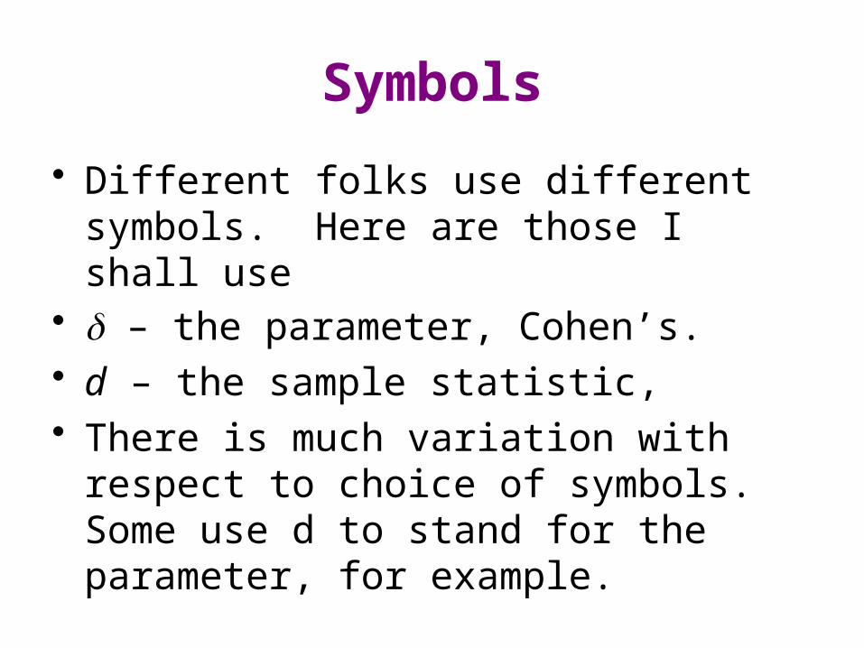
Symbols

• Different folks use different symbols. Here are those I shall use

• – the parameter, Cohen’s.• d – the sample statistic, • There is much variation with respect to

choice of symbols. Some use d to stand for the parameter, for example.

One Sample

• On SAT-Q, is µ for my students same as national average?

• Point estimate does not indicate precision of estimation.

• We need a confidence interval.

20.385.93

78.18

s

Md

Constructing the Confidence Interval

• Approximate method – find unstandardized CI, divide endpoints by sample SD.

• OK with large sample sizes.• With small sample sizes should use an

exact method.• Computer-intensive, iterative procedure,

must estimate µ and σ.

Programs to Do It

• SAS • SPSS

• The mean math SAT of my undergraduate statistics students (M = 535, SD = 93.4) was significantly greater than the national norm (516), t(113) = 2.147, p = .034, d = .20. A 95% confidence interval for the mean runs from 517 to 552. A 95% confidence interval for runs from .015 to .386.

Benchmarks for

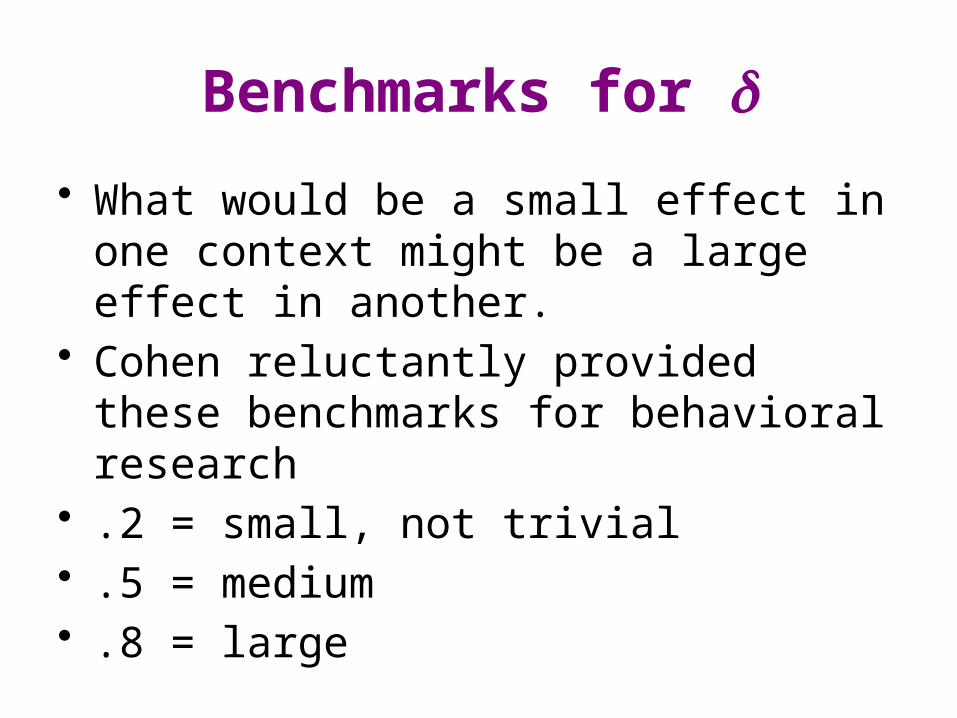
• What would be a small effect in one context might be a large effect in another.

• Cohen reluctantly provided these benchmarks for behavioral research

• .2 = small, not trivial• .5 = medium• .8 = large

Reducing Error

• Not satisfied with the width of the CI, .015 to .386 (trivial to small/medium)?

• Get more data, or• Do any of the other things that increase

power.

Why Standardize?

• Statisticians argue about this.• If the unit of measure is meaningful (cm, $,

ml), do not need to standardize.• Weight reduction intervention produced

average loss of 17.3 pounds.• Residents of Mississippi average 17.3

points higher than national norm on measure of neo-fascist attitudes.

Bias in Effect Size Estimation

• Lab research may result in over-estimation of the size of the effect in the natural world.

• Sample Homogeneity• Extraneous Variable Control• Mean difference = 25• Lab SD = 15, d = 1.67, whopper effect• Field SD = 100, d = .25, small effect

Two Independent Means

21

pooleds

MMd 21

)( 2jjpooled sps

N

np j

j

21

21

nn

nntd

Programs

• Will do all this for you and give you a CI.• Conf_Interval-d2.sas • CI-d-SPSS.zip •

Confidence Intervals, Pooled and Separate Variances T

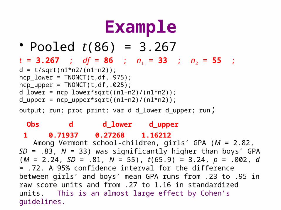
Example• Pooled t(86) = 3.267t = 3.267 ; df = 86 ; n1 = 33 ; n2 = 55 ;d = t/sqrt(n1*n2/(n1+n2));ncp_lower = TNONCT(t,df,.975);ncp_upper = TNONCT(t,df,.025);d_lower = ncp_lower*sqrt((n1+n2)/(n1*n2));d_upper = ncp_upper*sqrt((n1+n2)/(n1*n2));

output; run; proc print; var d d_lower d_upper; run;

Obs d d_lower d_upper 1 0.71937 0.27268 1.16212

Among Vermont school-children, girls’ GPA (M = 2.82, SD = .83, N = 33) was significantly higher than boys’ GPA (M = 2.24, SD = .81, N = 55), t(65.9) = 3.24, p = .002, d = .72. A 95% confidence interval for the difference between girls’ and boys’ mean GPA runs from .23 to .95 in raw score units and from .27 to 1.16 in standardized units. This is an almost large effect by Cohen’s guidelines.

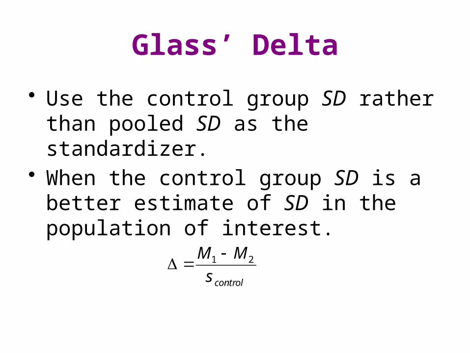
Glass’ Delta

• Use the control group SD rather than pooled SD as the standardizer.

• When the control group SD is a better estimate of SD in the population of interest.

controls

MM 21

Point Biserial r• Simply correlate group membership with

the scores on the outcome variable.• Or compute

• For the regression Score = a + bGroup, b = difference in group means = .588.

• standardized slope =

.33.861.

)487(.588.

y

xpb s

sbr

.332.86267.3

267.32

2

2

2

dft

trpb

This is a medium-sized effect by Cohen’s benchmarks. Hmmmm. It was large when we used g.

Eta-Squared• For two mean comparisons, this is simply

the squared point biserial r.• Can be interpreted as a proportion of

variance.• CI: Conf-Interval-R2-Regr.sas or

CI-R2-SPSS.zip • For our data, 2 = .11, CI.95 = .017, .240.• Again, overestimation results from EV

control.• 2

Cohen’s Benchmarks for and 2

• – .1 is small but not trivial (r2 = 1%)– .3 is medium (9%)– .5 is large (25%)

• 2

– .01 (1%) is small but not trivial– .06 is medium– .14 is large

• Note the inconsistency between these two sets of benchmarks.

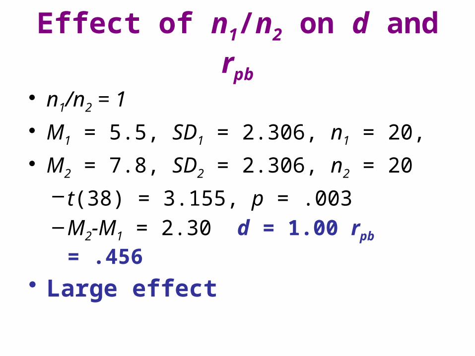
Effect of n1/n2 on d and rpb

• n1/n2 = 1

• M1 = 5.5, SD1 = 2.306, n1 = 20,

• M2 = 7.8, SD2 = 2.306, n2 = 20

– t(38) = 3.155, p = .003–M2-M1 = 2.30 d = 1.00 rpb = .456

• Large effect

Effect of n1/n2 on d and rpb

• n1/n2 = 25

• M1 = 5.500, SD1 = 2.259, n1 = 100,

• M2 = 7.775, SD2 = 2.241, n2 = 4

– t(102) = 1.976, p = .051–M2-M1 = 2.30 d = 1.01 rpb = .192

• Large or (Small to Medium) Effect?

How does n1/n2 affect rpb?

• The point biserial r is the standardized slope for predicting the outcome variable from the grouping variable (coded 1,2).

• The unstandardized slope is the simple difference between group means.

• Standardize by multiplying by the SD of the grouping variable and dividing by the SD of the outcome variable.

• The SD of the grouping variable is a function of the sample sizes.  For example, for N = 100, the SD of the grouping variable is– .503 when n1, n2 = 50, 50 – .473 when n1, n2 = 67, 33 – .302 when n1, n2 = 90, 10

Common Language Effect Size Statistic

• Find the lower-tailed p for

• For our data, p = .5,

• If you were to randomly select one boy & one girl. P(Girl GPA > Boy GPA) = .69.

• Odds = .69/(1-.69) = 2.23.

22

21

21

SS

MMZ

50.081.83.

24.282.222

Z

Two Related Samples

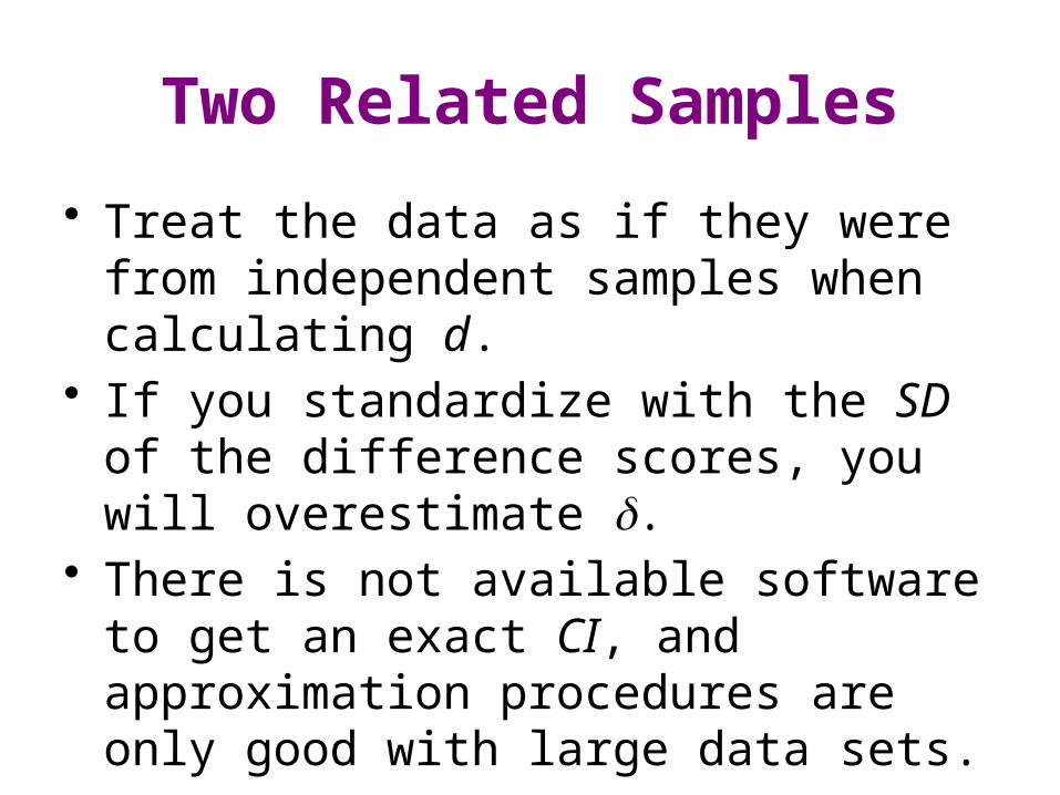
• Treat the data as if they were from independent samples when calculating d.

• If you standardize with the SD of the difference scores, you will overestimate .

• There is not available software to get an exact CI, and approximation procedures are only good with large data sets.

Correlation/Regression

• Even in complex research, many questions of great interest are addressed by zero-order correlation coefficients.

• Pearson r, are already standardized.• Cohen’s Benchmarks:

– .1 = small, not trivial– .3 = medium– .5 = large

CI for , Correlation Model

• All variables random rather than fixed.• Use R2 program to obtain CI for ρ2.

R2 Program (Correlation Model)

Oh my, p < .05, but the 95% CI includes zero.

That’s better. The 90% CI does NOT include zero. Do note that the “lower bound” from the 95% CI is identical to the “lower limit” of the 90% CI.

CI for , Regression Model

• Y random, X fixed.• Tedious by-hand method: See handout.• SPSS and SAS programs for comparing P

earson correlations and OLS regression coefficients.

• Web calculator at Vassar

Vassar Web App.

More Apps.

• R2 will not handle N > 5,000. Use this approximation instead:Conf-Interval-R2-Regr-LargeN.sas

• For Regression analysis (predictors are fixed, not random), use this:Conf-Interval-R2-Regr (SAS) orCI-R2-SPSS.zip (SPSS)

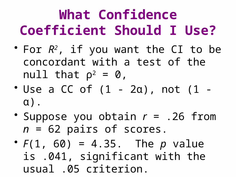
What Confidence Coefficient Should I Use?

• For R2, if you want the CI to be concordant with a test of the null that ρ2 = 0,

• Use a CC of (1 - 2α), not (1 - α).• Suppose you obtain r = .26 from n = 62

pairs of scores.• F(1, 60) = 4.35. The p value is .041,

significant with the usual .05 criterion.

Bias in Sample R2

• Sample R2 overestimates population ρ2.• With large dfnumerator this can result in the CI

excluding the point estimate.• This should not happen if you use the

shrunken R2 as your point estimate.

1

)1)(1(1 shrunken

22

pN

NRR

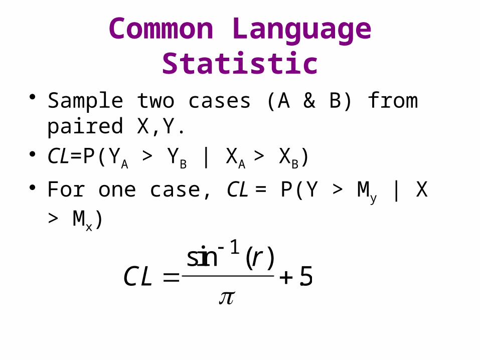
Common Language Statistic

• Sample two cases (A & B) from paired X,Y.• CL=P(YA > YB | XA > XB)

• For one case, CL = P(Y > My | X > Mx)

CLr

sin ( )

.1

5

r to CL

r .00 .10 .30 .50 .70 .90 .99

CL 50% 53% 60% 67% 75% 86% 96%

Odds 1 1.13 1.5 2 3 6.1 24

Multiple R2

• Cohen:

• .02 = small (2% of variance)• .15 = medium (13% of variance)• .35 = large (26% of variance)

2

22

1 R

Rf

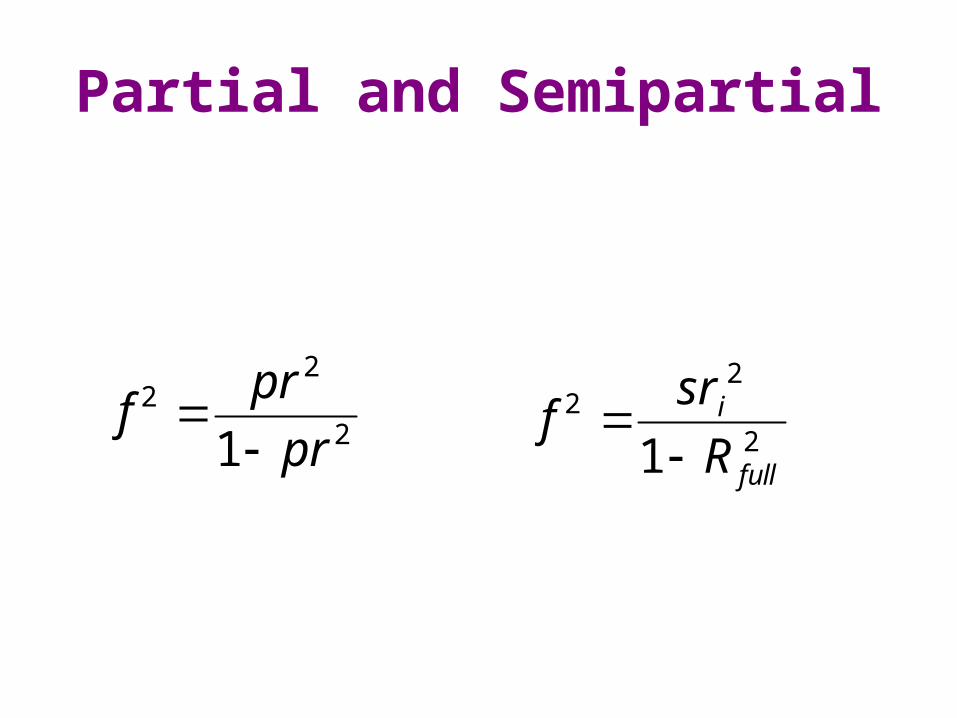
Partial and Semipartial

2

22

1 prpr

f

2

22

1 full

i

R

srf

Example

• Grad GPA = GRE-Q, GRE-V, MAT, AR• R2 = .6405

• For GRE-Q, pr2=.16023, sr2=.06860

78.16405.1

6405.2

f

191.16023.1

16023.2

f .191.6405.1

0686.2

f

One-Way ANOVA

• sdsdfsdsd

942.138

1302 Total

sAmongGroup

SS

SS

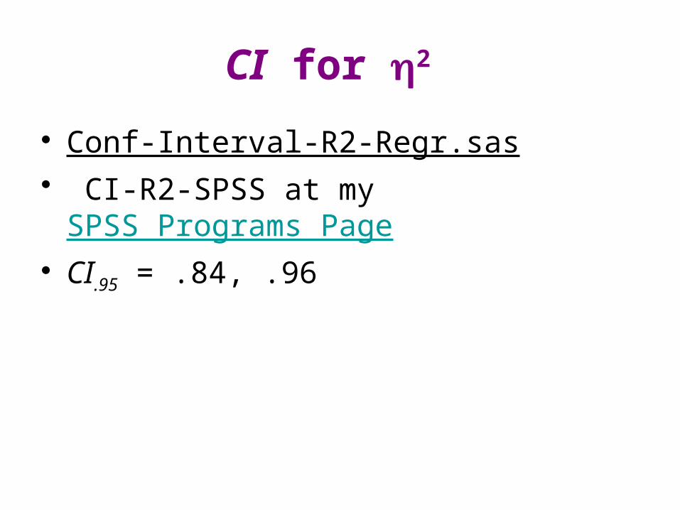
CI for 2

• Conf-Interval-R2-Regr.sas • CI-R2-SPSS at my SPSS Programs Page • CI.95 = .84, .96

2

• Sample 2 overestimates population 2 • 2 is less biased

• For our data, 2 = .93.

ErrorTotal

ErrorAmong

MSSS

MSKSS

)1(2

Misinterpretation of Estimates of Proportion of Variance Explained• 6% (Cohen’s benchmark for medium 2

sounds small.• Aspirin study: Outcome = Heart Attack?

– Preliminary results so dramatic study was stopped, placebo group told to take aspirin

– Odds ratio = 1.83– r2 = .0011

• Report r instead of r2? r = .033

Extraneous Variable Control

• May artificially inflate strength of effect estimates (including d, r, , , etc.).

• Effect estimate from lab research >> that from field research.

• A variable that explains a large % of variance in highly controlled lab research may explain little out in the natural world.

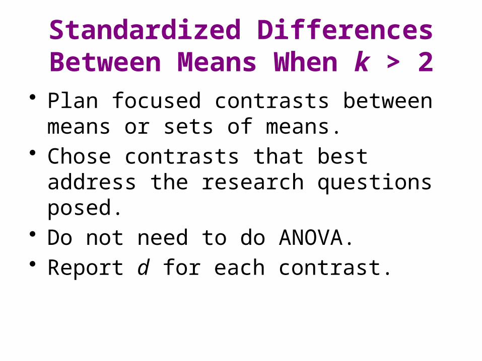
Standardized Differences Between Means When k > 2

• Plan focused contrasts between means or sets of means.

• Chose contrasts that best address the research questions posed.

• Do not need to do ANOVA.• Report d for each contrast.

Standardized Differences Among Means in ANOVA

• Find an average value of d across pairs of means.

• Or the average standardized difference between group mean and grand mean.

• Steiger has proposed the RMSSE as the estimator.

Root Mean Square Standardized Effect

• k is the number of groups, Mj is group mean, GM is grand mean.

• Standardizer is pooled SD, SQRT(MSE)• For our data, RMSSE = 4.16. Godzilla.• The population parameter is .

2)(

1

1

MSE

GMM

kRMSSE j

Place a CI on RMSSE• http://www.statpower.net/Content/NDC/NDC.exe

Click Compute• Get CI for lambda, the noncentrality parameter.

Transform CI to RMSSE

• The CI for lambda = 102.646, 480.288

• CI for = 2.616, 5.659.

nkRMSSE

)1(

CI → Hypothesis Test

• H0: = 0.

• cannot be less than 0, so a one-tailed p would be appropriate.

• Accordingly we find a 100(1-2α)% CI.• For the usual .05 test, that is a 90% CI.• If the CI excludes 0, then the ANOVA is

significant.

Factorial Analysis of Variance

• For each effect, 2 = SSeffect/SStotal

• 2: as before, use SSeffect in place of SSAmongGroups

• Now suppose that one of the factors is experimental (present in the lab but not in the natural world).

• And the other is variable in both lab and the natural world.

Modify the Denominator of 2

• Sex x Experimental Therapy ANOVA• Sex is variable in lab and natural world• Experimental Therapy only in lab• Estimate effect of sex with variance due to

Therapy and Interaction excluded from denominator.

• The resulting statistic is called partial eta-squared.

Partial 2

• When estimating Therapy and Interaction, one should not remove effect of Sex from the denominator.

ErrorEffect

Effectp SSSS

SS

2

Explaining More Than 100% of the Variance

• Pierce, Block, and Aguinis (2004)• Many articles, in good journals, where

partial 2 was wrongly identified as 2 • Even when total variance explained

exceeded 100%.• In one case, 204%.• Why don’t authors, reviewers, and editors

notice such foolishness?

CI for 2 or Partial 2

• Use Conf-Interval-R2-Regr.sas • Use the ANOVA F to get CI for partial 2

• To get CI for 2 will need compute a modified F.

• See Two-Way Independent Samples ANOVA on SAS

Contingency Table Analysis

• 2 x 2 table: Phi = Pearson r between dichotomous variables.

• Cramér’s φ = similar, for a x b tables where a and/or b > 2.

• Odds ratio: (odds of A|B)/(odds of A| not B)

Small Effect

• Phi = .1• Odds ratio = (55/45)(45/55) = 1.49

Medium Effect

• Phi = .3• Odds ratio = (65/35)(35/65) = 3.45

Large Effect

• Phi = .5• Odds ratio = (75/25)(25/75) = 9.00

Phi and Odds Ratios

• The marginals were uniform in the contingency tables above.

• For a fixed odds ratio, phi decreases as the marginals deviate from uniform.

• See http://core.ecu.edu/psyc/wuenschk/StatHelp/Phi-OddsRatio.doc

CI for Odds Ratio

• Conduct a binary logistic regression and ask for confidence intervals for the odds ratios.

Multivariate Analysis

• Most provide statistics similar to r2 and 2

• Canonical correlation/regression– For each root get a canonical r – Is the corr between a weighted combination of

the Xs and a weighted combination of the Ys• Other analyses are just simplifications or

special cases of canonical corr/regr.

MANOVA and DFA: Canonical r

• For each root get a squared canonical r.• There will be one root for each treatment

df.• If you were to use ANOVA to compare the

groups on that root, this canonical r2 would be

total

groupsamong

SS

SS _2

MANOVA and DFA: 1 -

• For each effect, Wilks is, basically,

• Accordingly, you can compute a multivariate 2 as 1 - .

• If k = 2, 1 - is the canonical r2.

treatment error

error

Binary Logistic Regression

• Cox & Snell R2 – Has an upper boundary less than 1.

• Nagelkerke R2 – Has an upper boundary of 1.

• Classification results speak to magnitude of omnibus effect.

• Odds ratios speak to magnitude of partial effects.

Comparing Predictors’ Contributions

• It may help to standardize continuous predictors prior to computing odds ratios

• Consider these results

Relative Contributions of the Predictors

• The event being predicted is retention in ECU’s engineering program.

• Each one point increase in HS GPA multiplies the odds of retention by 3.656.

• A one point inrease in Quantitative SAT increases the odds by only 1.006

• But a one point increase in GPA is a helluva lot larger than a one point increase in SAT.

Standardized Predictors

• Here we see that the relative contributions of the three predictors do not differ much.

Why Confidence Intervals?

• They are not often reported.• So why do I preach their usefulness?• IMHO, they give one everything given by a

hypothesis test p AND MORE.• Let me illustrate, using confidence

intervals for

Significant Results, CI = .01, .03

• We can be confident of the direction of the effect.

• We can also be confident that the size of the effect is so small that it might as well be zero.

• “Significant” in this case is a very poor descriptor of the effect.

Significant Results, CI = .02, .84

• We can be confident of the direction of the effect

• & it is probably not trivial in magnitude,• But it is estimated with little precision.• Could be trivial, could be humongous.• Need more data to get more precise

estimation of size of effect.

Significant Results, CI = .51, .55

• We can be confident of the direction of the effect

• & that it is large in magnitude (in most contexts).

• We have great precision.

Not Significant, CI = -.46, +.43

• Effect could be anywhere from large in one direction to large in the other direction.

• This tells us we need more data (or other power-enhancing characteristics).

Not Significant, CI = -.74, +.02

• Cannot be very confident about the direction of the effect, but

• It is likely that is negative.• Need more data/power.

Not Significant, CI = -.02, +.01

• A very impressive result.• Tells us that the effect is of trivial

magnitude.• Suppose X = generic vs. brand-name drug• Y = response to drug.• We have established bioequivalence.