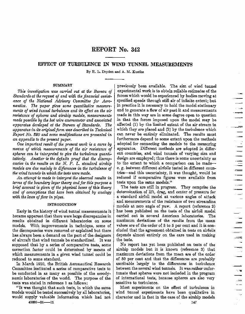
———. -.—-

REPORT No. 342

TURBULENCE IN

EFFECT OF

WIND TUNNEL MEASUREMENTS

By H. L. DRYDEN and A. M. KUETHE

Bureau of Standards

145

REPORT No. 342

EFFECT OF TURBULENCE IN WIND TUNNEL MEASUREMENTS

By H. L. Dryden and A. M. Kuethe

SUbLTIARY

This hrestigath uw carried out at f]lt?Bureau ofStandardsat #herequest of and m“ththe$nancial a@d-ance of the Nat&nud Adrhory Committee for Aero-nautics. The paper ties some quantitative measwe-ments of ~“nd tunnel turbulence and its efect on tha airresistance of spheres and air~hip mode.?i,measurementsmade posw”bleby the hot m“re anemometerand associated

previoudy been available. The aim of wind tumelexperimental work is to obtain reliable estimates of theforces which would be experienced by bodies moving at

-

specfied speeds through still air of Mnite extent; but ““-in practice it is necessary to hold the model statioriary

.—-

and to generate a flow of air past it and measurements.-

made in this way are in same degree open to question——

in that the forces imposed upon the model may beapparatus dereloped at the Bureau of Standards. The ! afTected(I)by the Iimited extent of the air stream inapparatus in its om”p”rur[form wa8describedin TechnicalReport No. 320 and some nmdijicdiom are presented inan appendix to the present paper.

One important remdtof the present work k a cww bymeans of u~hichmeasurement of the air resktance ofspheres can be interpreted to gke the turbulence quanii-tatkely. Another is the dejirde proof that the discrep-ancies in the results on the N. P. L. standard airshipmodels are due mainly to differences in the turbulence ofthe wind tunne18in which the testsu’ere mude.

An attemptis made to interprei the obserred results interms of the boundary layer iheory andfor this purpose abrief account is g-ken of the physicul baaesof this iheoyand of conceptions that hare been obtained ~ analogywith the laws of j?mc in pipes.

INTRODL’CTION

Early in the hietoqy of wind tund measurements itbecame apparent that there were krge discrepancies inresults obtained in different laboratories on somemodels. ‘With improvements in technique, some ofthe discrepancies were removed or excphined but therehas always been a demand on the part of the designemof aircraft that wind tunnels be standardized. It wassupposed that by a series of comparative teats, somecorrection factor could be determhed by means ofwhich measurements in a given wind tunnel could bereduced to acme standard.

In hlarch 1920, the British Aeronautical ResearchCommittee instituted a series of comparative teats tobe conducted in as many as possible of the aerody-namic laboratories of the world. The purpose of thetests was stated in reference 1 es follows:

“It vvasthought that such teats, in which the samemodeIe would be tested successively by all laboratoriesjwould supply valuable information which had not

41%30—31-11

which they ar; pIaced and (2) by the turbulence whichcan never be entirely eliminated. The rcm.hs mustfurthermore depend to some extent upon the methodsadopted for connecting the modeIs to the measuringapparatus. Different methods are adopted in diEfer-ent countriw, and wind tunnels of vary@ size anddesign are employed; thus there is some uncertainty asto the extent to which a comparison can be made-e. g. between ditTerentairfoils tested in Merent emm-trk-and this uncertainty, it was thought, wouId bereduced if comparative figures were avaiIable fromtests upon the same modeIs.”

The tests are stiII in progress. They comprise thedetermination of lift, drag, and center of pressure fora standard airfoil model at various angles of attackand measurements of the resistance of two streamlinemodeIe at zero angIe of yaw. A report (reference 2}has been published on the tests of the airfoil modelcarried out in several American laboratories. Themaximum deviations of the results from the meanvalues are of the order of 3 to 5 per cent and it is con-cluded that the agreement obtained in tests on airfoilsdepends ahnost entirely on the care used in makingthe tests.

No report has yet been published on tests of theairship modeIe but it is known (reference 3) thatmaximum deviations from the mean are of the orderof 50 per cent and that the diHerences me prcbablyascribable largely to the diflerencw in turbulencebetween the several wind tunnels. It was rather unfor-tunate that spheres were not included in the programof international tests, because spheres are also verysensitive to turbulence.

Most experiments on the effect of turbulence inwind tunnel experiments have been qualita~ive incharacter and in fact in the case of the airship models

147

—.-.—

.

.-..—

.—

.-=—

-—

.-

-. =

148 REPORT NATIONAL ADWSORY COMMITTEE FOR AERONAUTICS

the observed effecb have been attributed to turbulenceon the basis of a process of elimination rather than ondirect experiment. With the development of appa-ratus at the Bureau of Standards for the qurmtit~tivemeasurement of turbulence (reference 4), it becamepossible to study quanti tatively the effect of tur-bulence on the drag coefEcient of models. This workwas carried out .at the Bureau of Standards with thecooperation and flna.nciaI assistance of the NationalAdviscny Committee for Aeronautics.

BOUNDARY-LAYER THEORY

The discussion of the experiments d~cribed in thispaper will be phrased in the language of the boundary-layer theory of PrandtI (reference 5) and L-Nthere is noone article to which the reader may be referred for thenecessary information, it is desirable to state brieflythe eIements of this theory, It is well known that inthe greater part of the field of flow about any objectat the Reynolds Numbers encountered in wind tunnelexpedients or at greater Reynolds Numbers, the flowis approximately irrotational in character, and thedissipation of energy is negligible. The experimentallyobserved fact is that’ sc long m we do not enter theeddying wake behind the body, the pressurecmthe openend of a tube placed paraUeI to the flow (which is ameasure of the total energy per unit volume) remainsconstant throughout the field. The wake, extendingdownstream from the body, in many cases has a crosssection equal to or slightly greater than the cross sectionof the body at the begkning and increasesdownstream,but in other cases (airship hulh or finely tapered struts)the wake is very small. At least over the upstreampart of the body, the total-head tube may be broughtexceedingly close to the surface without observing anychange in its indication. The speed at the surface isknown to be zerc from the experiments of Stantonand his coworkers (reference 6), yet not far awayfrom the surface, the speed is observed to be relativelyhigh. These experiments indicate that the effect ofviscosity (at least over the upstream parts of bodies)is confined to a veqy thin layer. Prsndtl’s introduc-tion of this hypothesis, namely, that the field may bedivided into two regions, in one of which the effectof viscosity is negligible led to the so-called boundary-layer theory.

It was found by a consideration of the order ofmagnitude of terms in the general equations of motionof a viscous fluid that if such.a layer existed, its thick-ness must be of the order of magnitude of the squareroot of the product of kinematic viscosity and thedistance from the nose divided by the square root ofthe air speed, i. e., for air, if the speed and distancefrom the nose are taken as 1 ft./aec. and 1 foot, respec-tively, of the order of 0,15 inch. The equations fuml.lyarrived at for the steady flow of an incompreseible fluidin the boundary l&yer along a 2dimensional surface

whose radius of curvature is large as compared withthe thickness of the layer are as folIows:

(1)

(2)

(3)

whare u is the tangential component of the velocity, vthe normal component, x the distance measured alongthe surface, y the dietante measured norma~ to thesurface, v the kinematic viscosity, and p the pressure.As boundary conditions we have u =0, v==O at thoboundary y= O;u = U, the speed in the pot+mtial flowat y =6, the outer edge of the layer. Equation (1)states that the tangential acceleration of a fluid particleis produced by the resultant of the forces due to thepressure and the forces due to viscosity. -The term

omitted from the general equation is v L%” Equation

(3) is the equation of continuity. Equation (2) is

that. for the normal acceleration. The ~erm u av,ax

bv a% W)v ~-l ~~Z~ V~appearing in the general equations are

neglected, being of the second order, Equation (2)states that the pressuredoes not vary across the bound-ary layer. It is therefore the same as the pressure inthe potential flow outside the layer. Hence the pres-sure on the surface of the body is equal to the pressurein the potential flow at the outer edge of tho layer. Wemay then compute from the observed pressuredistribu-tion by means of Bernoulli’s theorem the speed at tlmouter edge of the boundary layer and thus obtain allof the data necessary for a solution of the boundarylayer equatio~.

The exact solution of the equationa of the boundarylayer. (equations 1, 2, 3) meets with great difficulties,although by great labor a solution can be obtained inany numerical case. (Reference 7.) An exact solu-tion has been obtained by Bhwius (references 8 and 9),by means of series developments, for the case of skinfriction on a thin flat plate of infinita breadth. In

this case ~ is negligible. The speed u increases

asymptotically to its limiting value U and hence noexact value can be assigned to the thic)mess of the

layer. & approximate value is 5.5J

~“ The drag

coe5cient, namely, the force divided by the productof velocity pressure, Mp W and area of the plate, comes.—

out equal to 1.33d

~~ wherez is the length of the plate

in the direction of the stream. The resistance of agiven plate therefore varies as U 1.6.

—

—

.

EFFECT OF TUltBULENCE IN WIND TUNNEL 3fEM~ 149 —

In the present paper we shall ha-i-elittle to do withthe ~~act solutions, but we shall attempt to carry thediscussion somewhat further by the approximationmethods developed by Karman and Pohlhausen.(References 10 and 12.) These approximations arebaaed on a new equation, an integral equation, obttinedas a fist integd of the differential equations previoudygiven or clerked directly from the principle of momen-tum. Because of the importance of this equation,known as the Kmrnan integral relation, we shalIrepeatits deri~ation.

The principle of momentum applied to steadymotion states that the integral of the flux of momentumtalien over any cbsed surface is equal to the resultantof the forces acting on the surface.1 Let us apply thisprinciple to a section of the boundary layer (l?igore 1)of thickness 6 and width &c. The mass of fluid enter-ing per second through a smalI element dy in theleft boundary of the swctiog is equal to p u dy and themomentum per second brought in is p u= dy. The

t total momentum per second entering through the

sa

left boundary is therefore p d dy. The momentum

per second learing through the section at the right is

J‘p uz dy+[$l P u%~v]ti. Some momentum

o

enters through the sloping upper boundary whose slopeexceeds that of the local streamhne. To obtain thismomentum we note that the totaI mass per second

J

zentering at the left is p u dy and the totaI mass per

0

seeond leating at the right isf ‘Ud’+[$r P“d’l

da The mass per second entering through the sloping

[41 pud’l&mdticeupper boundary is therefore ~

this mass enters with velooity U, the momentum persecond entering is

The time rate of increase of downstreamwithin the ~olume element is therefore

momentum

[LrP“’d’lti-u[:fPud’ld’oThis must equaI the sum of the downstream com-

ponents of all the forces acting on the surface of the

eIement. rThese are pt on the left boundary, – pfiL

+&(@ dir] on the right, p‘~ h on the upper sloping

boundary and –du.

()p .Ty ~.lj&con the lower boundary.

I A more precbestatement fsea follom- If anyfkeddad eurfecehe dewfkiwithins steady stream of 5nfcL the Ume mte of fnaease, within the surfwe, ofmomentum fn enY gken dlreetfonIseqnrdtothemm of the conmonents In tbetdlreoUon ofeJlthe forces e+MwontheErrU Ifh@f~.5uch eswr@hLamabsent or negIfgibIe,as theyere in the present iustence, the only form w be eondd-emd ore thma ecthg at the earfec% vi% ncmnel fmeee dne to hydrmtetic prsmrqand tengentlrd forcesdue to vkoue r.hwing.

I

ti

I

(ALk the viscosity). The total resultant force is ~

therefore –. ~du

()o!d%z-p ~y -o dx and the prinoiple of ---

momentum states—

~[~p”’d~]-~’~[~~~dy]=-’~ ‘--

“+-1-

Ve[ocifyudy ~

p6&—

I

(4) .——.-—-.:——

—

FIGmE L-FOMESon m demerit ofthe bounderY IWI .--

We now introduce a function q such that u= U– q*. —We tlnd

= –p Ug–p u&u8+P u;

M “d’*lHence

‘W ‘d’l-puwr’d’lp ug-2P=

+abd’l

S–d*+K($)po

“ I k the amennt by whfch the Iongitndtnal c&&I at enY dbtauee F from thesolid surfem is Ices then the S- of the Il!e4steam oubid% or the mttintioudne to the DMrlmitY ti the snrface.

--

-.-

—

—

---

—

—.-

—

150 REIPORT NATIONAL ADVISORY

= O,and hence the multipliers of 6on the two sides are

equal We have left, dividing by P, the Karmanintegral ralation,

=, rig()dy ..O(5)

To use this equation for the development of ap-proxim&te solutions, any reasonable assumption ismade as to the variation of g with y and the integraIrelation is used to give a dMerential equation for thethickness of the boundary layer. For example if wemake the rough assumption of a hear distribution,

= – ~ and the equation for ~is found to be

Ugd6 6U6dU VU—— .-—‘~d~- 6 dx 6

or (6)dll

The solution of this equation is readily seen to be

J8==l& ~zuwx (7)

and the force, F’z,per unit breadth across the stream, isgiven by

Uwxs~J‘* : ‘lPdxo

(8).

sIf we set ~zW’dx= I, the force coefficient, CF= @$%

is found to be

d~

ssVdxcF=& ~ ~

(9)

For the case of skin friction on a flat plate, U= con-stant = UO. Hence I= U2Z

(lo)

(11)

as compared to the exact solution C~= 1.33d $&”

.

COMMJ37PEE FOR AERONAUTICS

StiLIcloser approximations may bo made by assum-ing that g=a + by+ cy’ + d@, etc., determining thocoefficients by suitably chosen boundary conditions,

forexample uTUaty=~, u= Oaty=O, $= Oaty=6,

d% I d~ at~=; & Y= o from equation (l). Enough

b&mdary conditions are chosen to fix tho coefficientsin terms of & The integral relation then gi-rcs adiflerentiaI equation from which 6 maybe determinedas a function of z, the distanco downstream from thenose. The reader is referred to I?ohlhauscn’s paper(reference 10) for further examples.

SEPARATION

pen the pressure increases downstream, an inter-esting result is obtained by the use of four or more

terms in the expression for q. It is found that ~

may vanish and the flow near the wall reverse. Thcrfluid particles near the wall are dragged along by thefriction of Jhe neighboring particles but are retardedby ~~e pressure. As the boundary Iaym thickens theretarding effect prevails and actually causes a rovermdflow. Such reversal entails separation of tho flOW _

from the surface observed on cylinders, and onairfoiIe at the burble point. Tho boundary layertheory thus accounts for the breaking away of tho flowfrom the surface and states that the separation isdetermined by the dissipation of energy occurring inthe boundary layer,

EDDYING BOUNDARY LAYERS

The remarks made so far apply to boundary layersin which the flow is laminar. Experiment leads us tobelieve that the flow is more often eddying 2 as in thecase, of flow in piptw and the laws of laminar motiondo not apply. The experimental results on flow inpipes are assumed to apply to the boundary layer. Agenf@ account of the phenomena in pipes which aroof interest in this connection is given by L. Schillor.(Reference 13.) We may distinguish two values of theReynolds Number (product of mean speed by t.hodiameter of the pipe divided by the kinematic vis-co@y), namely a lower Reynolds Number, belowwhich any turbulence initiaIIypresent is finally damped

..-1The ,word turbrdemi fs commonly nse.i In thk rmmectlon. It h demmblo to

dfsthrgokh We tnrbnkrrm from the turbulence emxwntered In wind tunnel alrstreams, Tho dlfferenm h prfndpallg fn ordar of megnttrrdo although tho tur.bulanco in a wind-tnnnel afr Mwrn h lmpowd by a honoycornb or othw mews onthe flow from withcwt, wbw~ eddyfng flow, ae we dreU term It, artsoe from ani~~ ~tabj~ty. TM d~tln~tfor) be ma wu bo ap~fit~ by r~~ ~h~hnve seem a demonstration of Roynolde orfgfrmlexperimentwfthetreiuoeof color.In eddgfng flow the etream of mkx b verg IW.ptdlydlrluswl thrwrgirmut the wholetube. The turbuform to wfnd-tmrnal atr strmrm CorrWWnde W a Wavertng afluctuation of the Itr.reof color, a turbufencaof a dit?eront order of megnItrrde fromtbnt fn the tidytng flow rmd Imfmsd from wftbout.

Same Whore make the dlsttnetion by IMI@ disturbance” or %dffnl dfeturb.WI@”wham ww me “tnrbulan@” md (turbulent” WbOrOWe use ‘%ddytn&Mbnt we feel that the nee of the word turbidenm to deaezlbe the depmturm of wind.tunnel @rstrearnsfrornnnllorrnkyand--new Iswolfeatablblrod.Althoughtheuseof %u’bulencw” in both awe dom not fn ganaral c80s0 rnnfrrdon, we fravtthorrght it prefwebk tn tho tntW.fl of CbIIitYto u diffwoottams,

EFFECT OF TURBULENCE IN WIND TUhNEL MIL4SU3E.MENTS 151

out and the flow becomes laminar, and an upper Rey-nokls IXumber at which kminar flow changes toeddying flow. The value of the low Reynolds Numberis approximately 22000 (ScMers mhe is 2,320). Thedue of the upper Reynolds NTurnberdepends on theamount of init.ial turbulence. The turbulence mayenter the pipe in the body of the fluid or maybe setupby the form of entrance. The highest due of theReynolds Number at which laminar flow has beenobserved is 51,000 (Reference 14), aIthough in mostexperiments values of the order of 12jO00are the highestobserved. The results are summarized by SchUer asfollows :

“The result of the present work, in which the criticalReynolds Number is a function of the ‘greatest’disturbance present, gives the following picture of thestability relations of laminar and eddying flow ksmooth tubes. To every Reynolds Number above2,320 there corresponds a quite defkite amount ofdisturbance which is required to produce eddyingHo-iv. The higher the Reynolds Number, the smalleris the necessary disturbance. Against still smallerdisturbances, the Iaminar flow is stable. Be.Iow thelovier critical Reynolds Number, R =2,320, the kuninarflow is stable against any disturbance, however great..There, no eddying state of flow is possible; vorticespresent ti always disappear if gi~en su%icient time.”

We shall assume the results obtained for pipes toapply to the boundary layer, the thickness of the“boundary layer” in the pipe being the radius of thepipe, and the speed at the outer edge of the boundarylayer corresponding to the 6peed at the center of thepipe. Siice in laminar flow in pipes the speed at thecenter is twice the mean speed, the Reymolds hTumberformed from thickness of boundary layer and speedat the outer edge corresponds to the commonIy usedReynolds Number for pipes formed from diameter andmean speed. We agsume that there is a definite func-tional rdation between the Reynolds Number fortransition and the initial turbulence?

SKIN FRICTION WITH EDDYING BOUNDARY LAYERS

The skin friction on a plate When the flow in theboundary layer is eddying maybe estimated by carry-ing over the results of measurement of skin frictionin pip @eferenc~ 12 ~d 15). Experimen~ oneddying flow in pipes show that the force, F., perunit area of vd is gken by

(12)

where p is the density, U the sFeed at the center ofthe pipe, v the kinematic viscosity, and r the radiusof the pipe.. It is assumed that the same equation

1S&Q&s expdments sbmred that the afticd Ee.mwIds Nmntwr wss S.IWW themxne fm a tnrbulen= prodncsd tn a gken manner, dtbough fbs measmement ofturbulence we# not qnantitstIv&

applies to skin friction on a plate with eddying flowin the boundary layer, if U is interpreted as the speedat the outer edge of the layer and r is replaced by 6,the thickness of the boundary layer.

In eddying flow in pipes the speed, u, varies acrossthe cross section according to the law

(13)

where y is the distance from the wall of the pipe.This fornda fits the experimental observations mxryclosely except very near the center of the pipe and -rerynear the wd. By assuming the same distribution ofspeed in an eddying boundq layer, replacing r by 6,and by using the Karman integral reIation (5) togetherwith the value of F. from (12) substituted for

dq()—P ~u ~ which apphd only to laminar flow, the.-. .—

thickness, 8, of the boundary layer maybe determinedand F= evaIuated in a more useful form. We find

and the integraI relation becomes

-; +~ Ug= -o.045g(&y’ (14)

The solution of this equation is

Jfi6r4~l~m=0.2~9 $ri z pfl & (15)o

For skin friction on a plate U=conatant = UO

and

(16)

(17)

It should be noted that F., the force per unit area, is afunction of x. We are more interested in the averageforce per unit area, ~’, on a plate of length, 1, namely

J

11

70 F. dx which turns out to be

.—.—

.-

.—

—

.—

...--.

—

--

—

—

.-—

—-

.-—

(18)

The force coefficient, C=, is given by

where R is the Reynolda h’umber ~=

(19)

.-—

152 REPORT NATIONAL ADVISORY

The experiments of Wieselsberger (Cf. reference 15)on skin friction indicate good agreement with formula(19), except that a better value of the constant is0.074. In the calculations made in this paper oneddying boundary layers, we shd use the formula

(20)

SEPARATION WITH EDDYING BOUNDARY LAYERS

When the motion in the boundary layer becomeseddying, the phenomenon of separation is delayed.In eddying motion, there is a more thorough mixing ofthe air particles and the driving action of the outerlayers is greater. This delayed separation producedby the eddying mofion of the boundary layer is respon-sible for the great variation of the drag coefficient ofspheres and cylinders in the criticaI region.

DEFINITION OF TURBULENCE

Before it is possible to speak of the measurementof turbulence in wind tunnels, we must be able to givea precise definition, The defiition adopted is asfollows: The turbulence a a given point is taken to

$0be the ratio of the square. ot of the mean square ofthe deviations of the speed from its mean value to themean value. At any point in the wind stream, thespeed fluctuates with time about a mean value. Theturbulence is the mean fluctuation taken in a definitemanner and expressed as a percentage of the meanspeed. A turbulence of 1 per cent means an equiva-lent sine wave fluctuation of + 1.4 per cent from themean value.4

The adoption of this simple scalar quantity needssome justMcation since in theoretical treatments ofeddying motion it is found necessary to separate thespeed fluctuation into components. Experiment showsthat the mean speed is very nearly constant over thegre~ter part of the cross section of wind-tunnel airstreams. The shape of the distribution curve changesas we go downstream only in the vicinity of the walls.There are accordingly no forces acting between adja-cent layers in the core of the air stream and we mayassume that the fluctuations of speed are entirelyrmdom. In the neighborhood of the walls u closebehind the honeycomb, this amumption is not trueand the separate components of the velocity fluctua-tions as-d as their phase relations must be considered.To characterize tho air stream of a wind tunnel, weneed only to ‘consider tie fluctuation of the absolutevalue of the speed so long as we do not get close enoughto the honeycomb to be able to detect the honeycombpattern in the distribution of mean speed.

We need akw to discuss the space distribution of theturbulence for many investigators have supposed that

~Thie d6Wtlon difkra aomewhet fromthatsIveninReference 4. There, thedouble amplltude of the eqoivrdeut she wave was sIvea i. e: 2.S. Valum in Refemem% 4 should b+ divided by 2.S to be comparable with those given in the prwentpaper.

COMMI’I?17EEFOR AERONAUTICS

some space characteristic of the turbulence was theimportant facior, It has been suggested for examplethat the turbulence should be characterized by theratia of the diameter of an average eddy to the modcldiameter, a quantity related pmhaps to the ratio ofthe diameter of a cell of the honeycomb to the modeldiameter. We find no evidence to support this idea.Experiment shows (reference 4) that tho turbulence isvery nearly constant across the cross section in thoregion ,wherethemean speed is constant. It has furthcrbeen shown (reference 16) that turbulence may bointroduced. without effect so long as the turbulent airdoemot reach the boundary layer at the surface of themodel. Therefore unless the space distribution of t.hcturbulence across the air stream is such that hrgechanges take place in a distance comparable with thethickness of the boundwy layer, wo would not mpectthe space distribution tQ be an important ftictor. WCexpect the observed force to be gcverncd by the turlm-lence of the air enterimgthe boundary layer.

The square root of the mean square deviation ischoaan instead of the mean deviation for convenience,since the final measuring instrument is a hot wirealternating cuimmt milliammeter which gives this typeof mean.

DESCRIPTION OF WIND TUNNELS USED

There are thee wind tunnels at the Bureau ofStandards, all of which were used in this investigation.Sketches of the three tunnels are shown in Figure 2.The following brief descriptions will serve to supple-ment the sketches.

The 4!&foot tunnel is of the National PhysicalLaboratory type, octagonal in cross section, the 4!4-foot dimension being between opposite faces. TIMfsired entrance of the tuwel is about 4 feet long, theparaLIelportion 25 feet long and the exi~ cone 15 feetlong, The diameter at the propeller end is 9 feet.The tunrd room is 68.5 feet long, 28.3 feet wide, and18 fed.high, and is divided transversely near the exitend of the tunnel by a wail honeycomb, consisting ofpasteboard tubes 1 inch in diameter and 4 inches long,packed in a light framework, which is covered on bothsides by wire netting. This open honeycomb structureserves to damp out the swirl and eddies in the airstream asit returns from the fan to the tunnel entrancwA speed range of 25 to 110 feet per second is atiaincdwith the expenditure of from 2 to 75 horsepower. Thepropeller is 8 feet 11 inches in diameter and is drivenat speeds from 170 to 870 revolutions pcr minuta by adirect current shunt-wound motor. The tunnel is ofwooden construction on a shwl framework.

The 3-foot tunnel is of the Venturi type, circular incross section. The entrance cone is 12 foot long, theworking portion o feet long, and the exit cone 33 feetlong. The diameter .at the end of the exit cone and a~the front of the entrance cono is 7 feet. The room is

—

EFFEC?T OF TORBULENCEI IN WIND TWKKEL M?IAWRE303NTS 153 .—

103.5 feet long, 21.3feet wide and 14 feet high. The ~honeycomb at the tunnel entrance is of onequarter-inch wood, the cells being 3 by 3 by 12 inches long. A ~plaster fairingisusedin the entrance cone; otherwise the ~tunnel is of wooden construction throughout. The wMI ~honeycomb is identical in type with that of the 4%foot Itunnel but is installed near the entrnnce end. Speeds !up to about 240 feet per second are obtained with amotor rated at 100 horsepower. The propeller is :

curreqt motor. The matium speed obtained is _ _approximately 100 feet per seeond.

31EhiSUREXIENT OF TURBULENCE~

The measurement of turbulence as de&md in ~ pre- “-—ceding section was made by the use of tho hot wire

—...—

~emometer in conjunction with an ampli~er and.,—

apparatus for compensating for the @ of the ho t wire.The earl-yform and theory of the apparatus are given ‘=

:: I If 4.-........ ........

;::.i.,!7::!,,. ......-..--------

,

Ci-cdr secfbn fk#wqlkwt Wortighh3 Secfltw -

~“u MMeycomb

. L

k3zF&——

:9 $ !,:.-.?!.: I,

C&cub- =x?dim tFro@a.lf

Na27 n n n n n l-’

WV; ;U4#EU

8L!REAUiFSTAiWARDSWASWGTWJ D.C.

-1FIGmtE 2

S-bladed, and is rotated at speeda up to 1,000 revolu-tions per minute.

The 10-foot wind tunnel is outdoors end is of woodenconstruction. The cross section is circular and thelength of the tunnel proper is 92 feet. A faired entrancebell, 4 feet lorg, is foIIowed by a wooden honeycomb,ceIIs4 by 4 by 12 inches long. The cyhlrical motionis 50 feet long and the exit cone 34 feet long. Thediameter at the exit end is 14 feet 2 inches. The4-bladed, 14-foot propdler is rotated at speeds up to550 revolutions per minute by a 200 horsepower direct-

1in reference 4. Since that report was prepared, sev-eral import ant moditlcationa have been made in theinterwt of conmmienoel portability, and accuracyThese mo-tions are treated in an appendix to thispaper, whmh in itself forms a supplement to reference 4.A photograph of the -pMer amdaccessory apparatusin its modified form is gi-rti in F- 3.

The turbulence was measured at three sections ofthe 4%foot tunnel as indicated in Figure 2 and at theworking section of the 3-foot tunnel and 10-foot tunnel.The m~an -dues obtained are given in Table I.

.-.-

.—.——.

.—.-——

154 REPORT NATIONAI.J ADVISORY COMMITTEE FOR AERONAUTICS

TABLE IT&btimmte

LOAJon8-foot tunnel, working s~tion ------------------------- 0.6l@foottunnel, w'orking section ------------------------ LO4fi-fmt tunnel, do~t~ sation -------------------- 1.24~-foot tunel, worktig wction ------------------------- L6

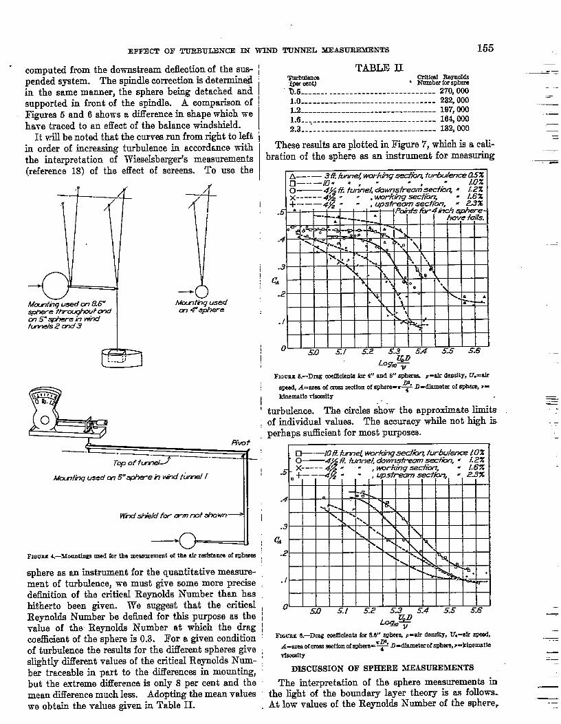
We have made tests on three spheres, of diameters 4,5, and 8.6 inches, at the five locations at which thoturbulence was measured, except that measurementswerd nit made on the hirge sphere in the 3-foot windtwhud because of the large ratio of the diameter of i.ho

4j4-foot tunnel, upstre& section ----------------------- 2.3 sphere to the diameter of the tunnel, Sketches of thoMany repeat measurements show that..the Precision suspensions used are given in Figure 4 and the rcsults

of the abo~e values is of the order of 0.1 to 0~2. It is I .of ~hemeasurements&e given ii Figures 5 and 0,

FIOCIIE 3

obvious that the efkcts of turbulence could be studiedover a reasonable range of values.

MEASUREMENTS ON SPHERES

The effect of turbulence in wind-tunnel measure-ments was first discovered for spheres and it has oftenbeen suggested that measurements on a sphere beused as a measure of turbulence. O. Flachabart (refer-ence 17) in a discussion of this proposal points out thenecessity of some standard method of suspension, ifmmparable results are to be obtained. We have notused exactly the same method of measurement through-out our sphere tests but Flachsbart’s results for thesuspensions used in our tests show that the differencesintroduced by this fact are small.

.

The 4-inch sphere was mounted on two wires ar-ranged in the form of a v in a pIane transverse to thewind direction. The force w-as computed from thodeflection of the sphere as a pendulum and the smallwire corrections were detembed by computation.Some i.xperiments were made on the 5-inch sphere inthe 4%foot tunnel on a bell crank. Correction wasmade for the motion of the scale pan and thg spindlocorrection was determined with the sphere mountedin front of the spindle. We prefer as a standardmethod the arrangement used for the 5-inch sphere inthe 3-foot and 10-foot tunneIs and for the 8.6 sphero inall cases, namely, a tail spind~c supported by twoV’S with a shielded counterweight, In this arrange-ment all wires are behind the sphere, The force is

155EFFECT OF TURBULENCE IN WIND TUNNEL MEASUREMENTS

.computed from the downstream deflection of the sus-pended system. The spindle correction is determinedin the same manner, the sphere being detached andsupported in front of the spindIe. A oompariaon ofFigures 5 and 6 shows a difference in shape which weha-re traced to an effect of the balance windshield.

It wiIlbe noted that the curves run from right to leftin order of increasirugturbulence in accordrme withthe interpretation of lVieseIsberger’s measurements(reference 18) of the effect of screens. To use the

tI

TABLE II~uIIItil CrftfcefReynoIds

i ● Nmnber for spherelLEi ------- .---.--------------------- 270,CKM3l.O--------------------------------- 232000lo--------------------------------- 197,0001.6--=------------------------------ 16%01302.3--------------------------------- 132,000

-- =

.-—

.-—

These results are plotted in F~e 7, which is a cali-bration of the sphere as an instrument for measuring

I1A —.— 3%!fMrk4wcwA-husedim fua.dc%zea5zlI&..-i-”-”;”;;-;- --;”- = ---0 ; . u?%

-cam Sed..bz “ 1.2%, e- 1I.oh I

I

m:;.---- iI

.-

Log*~:

FimxE 5.—Dras eoef%eknts ku 4“ end 5“ s@ere% P-afr dsnslty, U.=strsps@A=arsa of ems eeothn of sphere-r+D-~~ter of m, P“

1 kfnemstlo rIsccSfty

L~o—=

—

I‘ turbulence. The circles show the approximate limits; of individual V~USS. The accuracy while not high is

perhaps sticient for most purposes

-- -—

Ahr7ihq used m 5=qcAere n d thd f

Whdskkld fw mm rmts%Wn~

FIGuux 4—MountLogs usd for the m.eemrsment of the afr res&tsmm of mhme

sphere as an instrument for the quantitative measure-ment of turbulence, we must give some more precisedefhition of the crificaI Reynolds h’umber than hashitherto been given. We suggest that the criticaIReynolds Number be defined for this purpose as thevalue of the Reynolds Number at which the dragcoef%cient of the sphere is 0.3. For ~ given conditionof turbulence the results for the different spheres givedightly dMerent mdues of the critical Reynolds hTum-ber traceable in part to the d.itlerencesin mount~hg,but the extreme dMerence is only 8 per cent and themean difference much Lsss. Adopting the mean valueswe obtain the values given in Table II.

I

I —I

!

FIG~E 6.—Dreg coeCicfentr h S.6” s@=% P=* densftr,W.-k s’@@

A-area ofcrosssactfonofsphmw=r~ D-diameterof where, r.kfnemetie

vfscmfty

DISCUSSION OF SPHERE MEASUREMENTS

The int~retation of the sphere measurements in; the light of the boundary layer theory is m follows-, At Iow vaIues of the ReynokIa Number of the sphere,

—.—

.-

156 . llEPORT NATIONAL ADVISORY

the flow in the boundary Iayer is laminar and separa-tion takes place in a reamer governed by the laws oflmninar flow. As the Reynolds Number of the sphereis increased, the Reynolds Number formed from thethickness of the boundary layer and the speed at theouter edge reaches the value at which eddying flow be-gins at ecmo point upstream from the separation point,Seprtrationis then deIayed, the wake is smaller and theform resistance is decreased. The skin friction is sucha small part of the totsI drag that the effect of the in-creased skin friction due to the change from laminsr toeddying flow is inappreciable.

If the air stream is initially turbulent the change willoccur at a lower value of the Reynokls Number of theboundary layer and hence the critical Reynolds Num-ber for the sphere will be reduced by an amount whichincreases with increasing turbulence.

We can not make the interpretation a quantitativeone until more satisfactory methods are developed for

FwuaE 7.–CrIti&l ReyiioTds Nnrnbr of s@en% (at wblch C. (figs. 5and6) fs 0.9) as a furmtion of the tulwlencs

treating the phenomenon of reparation with eddyingas well as laminar boundary layers. An approximatesemiempirical treatment is given by Ono (reference 19)but Tollmien (reference 20) questions the legitimacyof the approximations used.

MEASUREMENTS ON STREAMLINE BODIES

Having obtained a very good correlation betweenmeasurements on spheres and the turbulence as mess-ured by our hot wire anemometm and associated appa-ratus, experiments were begun on streamline bodies.The fit model used was a bomb model known asIQ-12 which we had at hand. 11’ewere astonishedto &d no large eflect in view of the results on theN. P. L. models in diflerent wind tunnels, for we hadexpected that generally similar results would be ob-tained on dl streamline bodies. The actual bombmodel departed in several apparently minor respectsfrom a good streaniline body and tie therefore made a.wooden repIica without protuberances of any kind,The shape of this replica is shown in Figure 8 and theresults of measurements of the air force at the fivemeasuring stations are given in Figure 9. These

COMMITPEE FOR MKRONAUTICS

curves show certain s~hmatic changes but practicallyall of the points are within 10 por cent-of a mean curve,

Th&forc~ were measured by swinging the model onfour wires arranged in two V’s from the nose and tail,meas~ng the deflection at several wind speeds, theweightl and wire lengths, and computing the total dragof model and wires. The drag of the wires, amountingto about 75 per cent of the drag of the model, wascomputed, since we have found this procedure to giveaccurate results. To minimize errors due to the cor-rection for the wires, we have used the same wires atall stations in the 4x-foot tunnel and in the 10-foottunnel. In the 10-foot tunnel, the model was hungfrom an auxilia~ frame supported in the wind stream,

-““’0.0125i%-=+

.469 ff.

R-Q-/2~o Oftruss--secffion ~08;:;?&flghMUX.diumefer

/0;3330 i

MEL. shorf modelVolume

.Ao.W851W

‘ (p&i7# 0.2677 r%’

hfux.o%meier2.3340+7.0.3500 r%

. . .—

N.EL. long modelVo/ifme .0./888tw(vc&7#’1’ 0.3291ff.’

2.8600 B.Mox. diomefir 0.3500 e.

FIGURES.—tiitudlual sectloua of bcdies ofmvolutlon onwhfch10Mmwe-ments were made

Care must be taken in the interpretation of curvessuch as are shown in Figure 9, The observations aremade under such conditions that the forces and speedsare subjsot ta errors of roughly constant absolutamagnitude. The percentage error is therefore muchgreater at the lower speeds. Under thaw conditionsa plot of coefficients may prove misleading unk.ss oneremembem continually that the experimental errorsare diflerent in different parts of the diagram, Weestimate that the probable errors range from some13 per cent at a speed of 20 ft./see. tQ perhaps 2 or 3per cent at a speed of 100 ft./see.

No Z&rec$ons hav6 been applied for pressure drop,because we do” not believe that the method of cor-rection is as yet well established. We give neverthe-less the data required for making the correction.Table III gives the mean decrease in static pressure perfoot Iength divided by the velocity pressure for theseveral stations.

EFFECT OF TOEBUIJ3NCE IN ‘— ‘–—- ‘— ‘—–-—--–- 7 E*

TABLE III

Station PreSSRS drop

Moot ------------------------------- cLoo710-foot ______________________________ .0024}&fmt, domtram ~ction ----------- .00354~-foot, worHng*ction --------------- .CK)754%-foot, upstrsam section -------------- .0035

The dume of II-Q-12 is approximately 0.077cubic foot and the area of cross section, which is usedin defining the drag coeflkient for this model, is 0.0872square foot. Hence the corrections for pressure dropapplied in the usual manner to the coefficients ofF~ure 9 are to be found by multiplying the values

of the pressure drop given in Table III by - or

0.SS5, gking 0.0061 0.002, 0.003, 0.007, 0.003, orapproximate~y 10, 3, 5, 12, and 5 per cent for the

CA

om40w&wlm fa~Uo,l%/sec-

0 210 420 6= 840 1050 1260 f470Reynak%s Number x f04

FIGmI 9.-DIs.g memcknts for D-Q-19 W-n replfea. P-* d-b, -C*air epeed, A-area of cross sectfon (meshnnm S@fOd, Reynolds h’mnbec-

+ where [ k the length of mod~ M F is the kfnenmtfc vfscmfty

se~-eralstations. The application of these correctionswould not change the conclusion that the effect ofturbulence is smti compared -with the magnitude ofthe discrepancies found between the results on theN. P. L. mod& in the se~eral wind tunmds.

It was obviously desirable to pass immediately tomodels which gave a hwger drag coeflkient in somewind tunnels than in others and vre accordingly con-structed a wooden replica of the short airship model ,used in the A’. P. L. comparative tests. The resultsof a large number of runs are shown in Figure 10.Although it is difEcult to accurately measure the smaIIforces, there is clemly a very large difference betweenthe measurements at. the upstream and downstream

-. .-—

sections of the 54-inch wind tunnel. The variationmay be attributable in part to a change in the charac-ter of the surface of the model or to a change in shape

mtm

w-6ma

a, 17!/sec-0 .293 596 660 /!73 1455 17m 2U53

Reynolds N&e.- X k?-3

FIGGM 10.—Dreg eo?fiht.s for wodsn replica Of N. P. L. Short ~~ P-*

derdty, W.-air qxx?i, ReynoIds Nrunber+ WiW8 1 h the Iensth of thew, snd wh ChakbOlllltfC -ty

of the model inasmuch as the t&s covered a consider-able period of time. TO exclude this complication sofar as possible, mnmgemente were made to use theU. S. Na~ replicas of the N. P. L. models. The

—-— 3i%fLunA tmnkiiysedkhr. furbdfs%cea5:k—--—lo = . .O—.4% R. ;u/%d, &.w?sbm&fti : j:;

“ ,wa-ki-rgsecfti:-==% : - .unsi%-eumsectioh. - #i3z

.m4

c,

.Oa

.016

Ozu+wsowlm LamL&.&.3ec.

o 293 566 86o 1!73 /465 176u ZW53Reynolds Munber x h2+

FIGCEX 11.—Drsg mefEidenfs for metal replica of h-. P. L. -short modd P-ak

density, U.+ speecL R&ncdde Numben-=~J where t fs theleuth of themod+ mxl r & the Mnenatk vfsccdty

nominal dimensions of the modeIe are gi-ien in Table IVand the form is shown in Figure S. The resuk ofmeasurements of the drag are shown in Figures 11and 12. ●

- :.-=— —-——

—

—

=—.—

-

-

.

.

.

-

.

REPO13T NATIONAIJ ADVISORY COMMI!P1’EE FOR AERONAUTICS158

.036

.032

.(22W

.qr

.G24

.CE’o

.016

1 20 40 60 m 100 m Wa, ff/kec.

o 360 720 1080 1440 /800 2160 .2520Reynolds Number x/0-3

FIGURE 12.-Dreg we!llofenfa for metal repIleaof N. P. L. long model, p-ah

denefty, W.-air spwd, RejmoIda Number=~J where f fe the length of theIuodeJ end r fe the k!nematfc vleeoefty

TABLE IV.—NOMINAL DIMENSIONS OF U. S. N,REPLICAS OF N. l?, L. MODELS

Dtsteneeala:ng

ad:%

LW3

kgZama.oal8.am4.ml&mOd.fMI7.marm

1; EIL (0312mIL mIt mI&mm. m320XIS4.mZ&m!2a.dw23.015

ii%!n.fco32’wa34,316

hort modelman radios

a4e!.0s3.Wo.926

L LML2$0

::

L 7231.w

;!

2.03S.210121012.095!zOE4L 049L 771

HiiJ

%o“

hng modallW radfue

o...&d.927

1.Ha1.%21.421

:;

LmL W2(L91z 073

H%21M.21012 m2 la)2.wZ.oailL 909LW4Lb93

L 226L 018.617. awl

o

We may sum up the experimental n%ults on theeffect of ~urbulen~e on th~ resistance of streamlinemodels by saying that some modeIs show small effects,others show large eflectsj and that the large efTectearecofied to a certsin range of values of the turbulence.For example, the N. P, L. models show small effectsif the turbulence is less than about 1.3 per cent, largeeffects if the turbulence is greater, the effect of in-creasing turbulence being to increase the resisttmce.

We have then an explanation of the resuIts of theAmerican tern%on these models. The old variable

density tunnel was very turbulent as indicated by tholow value of the critioal Reynolds Number for spheres(about 94,000, Cf. reference 21). In agreement withthis indication, the measured drag of the airship modelswas greatmt in the variable density tunnel. (Refer-ence 3.) At the other extreme, the lowost vahms ofthe measured drag of the airship models were obtainedin the 3-foot and 10-foot wind tunnels of the Bureau ofStandards, which have snd turbulence. In tho nowvariable density wind tunnel the turbuhmce has beengreatiy decreased (reference 23) and it would bo ex-ceedingly interesting to determine whether the airshipmodels now give much lower drag coefficients,

DISCUSSION OF MEASUREMENTS ON STREAMLINEBODIES

The experimental results on airship models leavo onoin a very confused state of mind as to the interpreta-tion oLmodel experiments on airship hulls and as tothe explanation of the puzzling feature that the eflectsare hrge only for some models over a certain range ofvalues of the turbulence. We do not desire to leavothe subject in this state and we believe that theboundary layer theory as we have outlined it willaccount for the observed facts. Because we arehandicqped by the absence of methods of exactmathematical treatment, ye can only give a discussionbased ,og rather crude mathematical approximationswith t~e hope that the reader will obtain sonm sug-gestion as to how the observed results may follow fromthe boundary layer theory.

We tit determined experimentally th~t the phenom-enon of separation does not enter. This was done byplacing ~ thin fdm of oil on the surface and noting thatthere was no region of reversed flow. Wfi thereforeexpect that the ~ormresistance wilI be small, In fact,press~ have been measured on a model which issubstantially the N. P. L. long model (referenca 22}and it was found that the form resistance was prfic-tically zero. In other words, the observed resistancois due almost entirely to skin friction. We shall adoptthis assumption and attempt ta calculate onIy the skinfrictiorl.- We ,propose to compute the akin friction of tho

‘(equivalent flat plate, ” i. e. on a section of a two-&nenQonal pkme surface, the width of the section at . .,,a give&-distance from the front edge being equal tothe circumference of the model at the same distancofrom the nose of the model, and the speed at a givendistance from the front edge of the plate being thesame &s the speed computed by Bernoulli’s theoremfrom the pressure distribution at the same distancefrom the nose of the model. We shall identify theskin friction on the equivalent plate with the reaistancoof the model. The following assumptions aro impliedin the above procedure.

L No distinction is made between dist.ancsaalongthe mrface and distances along the axis.

EFFECT OF TURBUIJCNCE IN WIND TUNNEL MEASUREMENTS 159 _

2. The cosine of the angle betw-een any surface ele-ment and the axis is taken equal to unity.

3. The thickness of the boundary layer at a givenpoint is assumed smaII compared with the radius ofcross section of the mocM at the same point (obviouslynot true far back on the tail).

4. The equations of t~o-dimensiomd flow are used.For the computation of the point at which the flow

in the boundary layer changes from laminar to eddy-ing, and for the computation of the sldn friction onthe part of the surface for -which the flow in theboundary layer is .laminar, -we use the formulas ofequations 7 and 9. These are based on the use of alinear velocity distribution in the boundary layer andthe integral rdation of Karman.

For the computation of the skin friction on the partof the surface for which the flow in the boundary layeris eddying, we use equation 20 together with an assump-tion made by Prandtl (Reference 15) in connection withskin friction on plates, namely, that the force is thesame as if the flow were eddp”ng from the beginning.If the flow were eddying from the beginning, the co-efficient C2,for a surface of length lZ in a stream ofspeed UO,would be ghen by

For a surface of length ?I, the.coefficient, c1is gbren by

— where R,=w.0.074

c’= RI% v

Hence in the fit case, we may find the desired averagecoefficient, c, for that part of the surface between 11and 12(both {1 and la beiig measured from the nose)by stating that the weighted average of C1and c mustbe cZ,or

cJ1+c(&-ll)=dawhence

We add another to our formidable Iiet of assumptionsand approsirnations by not considering the -mriationsof the speed at the outer edge of the boundary layerin this computation, taking the wind tunnel speed, T-Jo,to compute C2.

We are now prepared to compute the skin frictionon the N. P. L. long model for wind streams of differ-ing amounts of turbulence in accordance with the ideasoutlined in the section on eddying boundary layers,name~y, that to each degree of turbulence there corre-sponds a different value of the critical Reynolds A1um-ber of the boundary layer for which the flow changes-.from laminar to eddying. The -dues of ~ computed

by Bernoulli’s theorem from the pressure distributiongiven in Reference 22 are shown in Fi.m 13. Weprefer to write equation (7) as

(22)

where1 so‘~‘dx.

==; lOO Uo(Q)

(23)

We note that the Reynolds Number of the bounda~layer, Rs, is

~’-”-’+(a(a’ forN. P. L. ImxzmoM wmputed from presmre

dfstrfbutirm of B2fsrsmca 22

‘0 Z he Reynolds Number 6 of theIntroducing R= y~ t

model, where 1is the length of the model, we tind

R6UgK-—. — /—JEUOJ1 “(25)

U’a

()Figure 13 shows a plot of ~ vs z. The value of K

was found by graphicaI integration as a function of x,

and from the values of K, Ion of x, which$; as a funct.

ia plotted in Figure 14. Equation (9) for the laminarforce coefficient may be written

We shalI eventualityneed the contribution to the forcecoe.fikient, 0, of the model defined in terms of (roI-ume) ~, for which purpose CFmust be multiplied bythe surface area, A=, of the model from the nose to the

I TM reader shculd note the ose ofthakwthof the model Mead of (vofume)lnfn the definition of R. It wflI he spprecfstad thst the hmsth E5wea betterkfs dtom-n.

.=

-

—

—

.-

—.<

.—

.-—

—

—.-

.=-.—

--

160 REPORT NATIONAL ADVISORY COMMITI’EE FOR AERONAUTICS

point x, and divided by (volume) ~. As before, vieintroduce the Reynolds Number of the general flowtmd write ?-T

x, ?%

FmtIEWIL-8,LWJ ,Vol)mCPA; @[or N. P. L. long model, RF fe Reynold

NumbeJ of lwundary Iayer d a dlstence z from the now, R fe the Rey.noble Number of the body, Cr k the average lamlnar ooefilofent of frio-tIon, A, h the eurfaw erea of the model tinr the nose to the point r

This quantity, which is to be di~idcd by @ to givothe laminar .coptribution to the total force coefficient.,is plot@d as a function of z in Figuro 14.

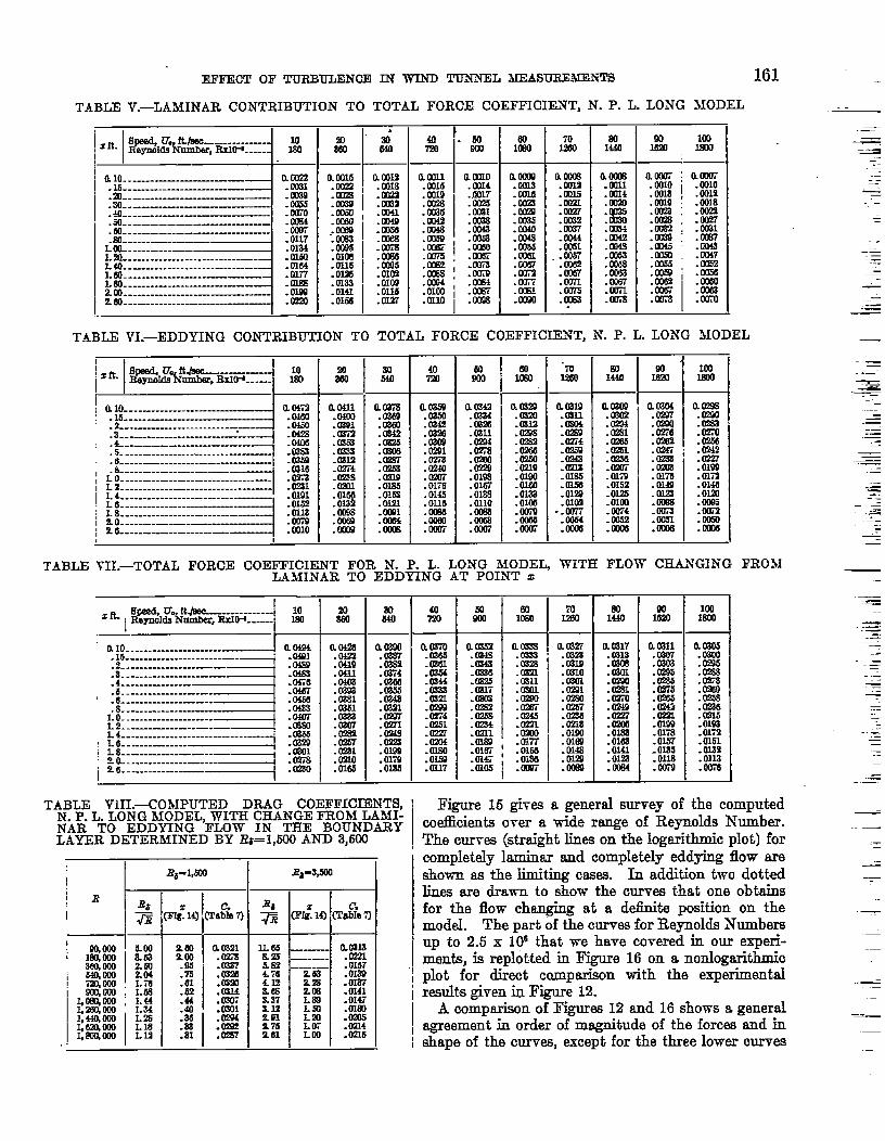
We next compute a table showing tho laminar con-tribution to the total force coefficient for varying Rand z, a table showing tho contribution of tho surfacobetween x and 1 for which the flow is eddying (com-putd” from Equation 21 by nmltiplying c by tho sur-face area and dividing by (volume) ~) for varyingR and z, and finally a table of computed total forcocoefficients (adding corresponding ontrics in the firsttwo tables) for varying R and z. larts of those tablesfor the N. P. L. long model are given in Tables V, VI,and VII, Table VII permits the easy calculation ofthe ti”tal drag coefficient, when the point at which thoflow changes from laminar to eddying is known. If,for example, the change always occurs at a llxod point,values are taken from the horizontal line correspondingto that point.

&sum@ the change from laminar to eddying flowto occur when the Reynolds Number, R?, of the bound-ary layer is equal to 1,500, 2,000, 2,500, 3,000, and3,500 we find z from Figure 14 and compute tho cur-rcsshown in F~re 15. The computations for R~ equal .to 1,500 and 3,500 are shown in part in Tablo VIII.

Reyn& &umber, R

FIOUM 16.–Comput@3 fi~g coallairmts for N. P. L. Iong mtiel forflow ohrmglngfrom ls.~nm h eddyfng under dlflerent condhions. Upper l[ne Ie fw eddying - -flow throughout, Io’irerllne forhrfner flow throughout. The dotted Hnwere for trerreftlon at the Indicated dkdenew from the nase. The ctrrvesere fortrerrd-

tfon at the veluw of the ReynoIds Nnmlmr, Rd, of the bonrrderyIayq indimted C,-M~~w-) p-rdr deuefty, U.-efr epeed. R-~ w ere 1 hu.{ hthe length of the model end Pthe klnernatfc vfmoelty

EFFECT OF TURBULENCE ~ WIND TCIN?XEL MEASURE_iS

TABLE V.—LAMINAR CONTRIBUTION TO TOTAII FORCE COEFFICIENT, N. P. L. LONG MODEL

161

!%t

t

1%0 Ix10

am amm.lm13 Ju#.W16.m .m.0G2Q .W27-w .013$4.lm40 .cml’.00is :%.CM3.OwU .-0057.0027.00i2 %J.CTi. as!. .007s.m!ao .=

1!!0I &k&l

Ma& O.cooi ; Cm&

:~ I .~.m4

%iJ %J : %J.W .- : Xl&.CM .0)45.WS .C150 .m47.0M9 .MKi .-.OMa .U19a ; .00s6.W37 .UM2 .DM1.m .WM .M63.C)is .M73 .m

+

ale---------------------- MK12&.M----.---.-.-.-–.–---–—-m------------.---.---.-— .Cm9AM--------.---.–-.---–-– .00M.W---.–--..--..--..--–-–.-— .Ooio.a----------------------------–– -wm-----------.-------..--.. ---.-— .Om.30___________ .mu

LW_...-–-.-—– .0134L% . . ..--. ---. -.--..-... --..-—. .mLti----------------------------- . ole4La------. --.. ---. -..-––—-— . OlnL~------------------------- .m!2w---.--. ---.. --.. -—–-— .OM12cO--—.--.----— .m

amu aano. 9X5 . on4.Cl19 .m~

.M25:%% . ml

.Oms:% .W

.@.w4

.0100 I

.O11o I .Mw9

——

-..=

T.4BLE VI.—EDDYING CONTRIBUTION TO TOTAL FORCE COEFFICIENT, N. P. L. LONG MODEL

1%“io& i%&aom.&w.0391.Cai2.mm.cm.0312.02i4.IE%

: FM. o13a-m.Owu.(33)9

ElI I racm sons.m

%% .-.0276 .0270.0m2 .0256.(Q47 i .0242.0233 .0227.m)a . OIQE. om . cm2. OM .0146.0123 . OlalNC& .CW5

.Wi2.Om .mo.mm .(m)

mm-..-.-.-...-.----–--—-—– a 04i2. is-----–-–---.---–– .W31.2--- –- —.–--------.-.. -–-–--—.3-- .----------. -.-... -.-. -_---_d :%

aa342.0234.m.ml.02a4.om.om.0229.O19S.QI&l.Om.OIlo.cKm.W.mm

AL-.––----_...- ...._--_._+ S&

::========= :%. k -------—--—-—-

1LO-..-. –--–-. –-.–-..-––-—-— .0273L 2--.-. -..----—-.---.–—--— . O!ulLo-----------------------

4

. 019LL 6--.-_ —------L8--.-.----–----- .–-.--––-— %!Lo---—-——-— .Ooie2 6------— ------- . mlo

—

TABLE VII.—TOTAL FORCE COEFFICIENT FOR N. P. L. 1LAMINAR TO EDDYING .

3NG MODEIT POINT x

WITH FLO CHANGIIS FROM

.—=

--. —-.—

.=—

& 1%aom.Wo7.030a.@m.om.om.E&s.o!m.ml.OIQa.OIis:E.Olls.00i9

A%amw.ccoo.0205.0%8.Oza.Om.0238.(3U6.0215. Om. Oliz. am:p;.mi6

a~o-----------------------_----J.15--..-..-..----------..—-.2_-.........------.s......-.-....-...-–— ===i.4.-.....–...--.5-------------------.6--. -..---. -.--—–-. s-----------

L 0- . . . . . . . . . . . . . . . . . ..-L 2.-.—..—.--–--—Lo------------------------

! Lo-----------i L 8--–--—–--——-: 20-- . . ..- . . . . . -------‘ 26--.-------–

—---.-—.-

TABLE VIII.—COMPUTED DRAG COEFINCR3NTS, ‘ Figure 16 gives a general survey of the computed _N. P. L. LONG bfODEL, WITH CHANGE FROM LA3iI-NAR TO EDDYING FLOW IN THE BOUNDARY coeflioients o-w a wide mug-e of Rewelds hTumber.LAYER DETERblINED BY Rz=1,600AND 3,500

—The curves (straight lines on-the log&thmic plot) forcompletely laminar md completely eddying flow areshown as the limiting cases. k addition two dottedlines are drawn to show the curves that one obtainsfor the flow changing at a dchite position on themodeI. The part of the curves for ReymoMs Numbersup to 2.5 x 1(Y that we have covered in our experi-ments, is replotted in Figure 16 on a nordogarithmicplot for direct comparison with the e~erimentalresults gi-mn h Figure 12.

A comparison of F~w 12 and 16 shows a generalagreement in order of magnitude of the forces and inahape of the curv~, except for the three low= curves

--=R*-l@Ll I R~.3ym

1

IB

r*fiO q

ao313.0221.0137.0139.01a7.0141.0147

:%%.0214. O!m

I—

1!Z60

t: :OJ2.m:% .75

.6-LL68 .62

.44M .40L% .36L13L19 :%

,- ——

162 REPORT NATIONAL A.IWISOEY COMMITTEE FOR AERONAUTICS

of Figure 12 below 50 ft.[see, In order to account for Ithe observed shape of these curves and in view of other ~evidence that will be presented later, we have been ledto the assumption that the flow soon becomes eddying ~behind the maximum cross section or speaking more ~

.034 U II{AN I I I RI I t 1 I i I

0261*

I1

.030

j1

Cv I

.0221:

+%+ k

I‘- ‘x-1.6

100 120 140~, ff./sec.

36 72 fo8 “f44 180 216 “-252ReynoldsNumber x10-4

FIGURE16.—RepmduotIorr of a part of Ffgnre 15 on a nordogarithmIo srde wfthaddklonal orrrves for trandtion from Iaminar W eddying flow at ayehlod d!.stnncca tim the nose

exactly that the contraction of cross section introducesturbulence, producing the same effect as any upstreamturbulence on the flow. We do not think it unreason-able to suppose that the necessary contraction in cir-cumference and increased thickenirw of the

point reaches 3,500 as indicated by intersection withthe curve for R6= 3,500. We then follow tho curvofor RJ= 3,5oo. A consideration of Figure 16 on whichseveral curves for diflerent points of transition medotted in will show how the experimental curves canbe fitted by a proper choice of point of transition curveand G= constant curve. The transition from onocurve to another is undoubtedly not “assharp as indi-cateil by this simple analyaia.

There is one other feature of the curves of I?iguro 12not yet accounted for, namely, the fact that for turbu-lence below about 1.3 per cent, there is apparently noeffect of turbulence. WQbelieved at first that this wascaused by the disturbance from the supporting wiresat t& nose introducing a turbulence of approximatdy1.3 per cent, so that aIthough the turbulence of thoair stream was reduced below this amount, the bound-ary layer was always subject to the approximatelyconstarit turbulence introduced by the wires. If thisinterpretation” is correct we should be able to obtainlower coefficients in the 3-foot wind tunnel by elimi-nating the disturbance at the nose. I?iguro 17 showsthe results obtained by mounting tho wooden replicaof the N. P. L. short model on a tail spindle simihtrto the sphere mounting (fig. 4), compared with resultson the same model and tail spindle with the front Vat the nose, The effect is not large although the resultswith the V at the nose are somewhat,higher and scatlcrmore than those with all wires behind the model,

boundary layer resulting from the re~uctionin cross section of the body does not takeplace smoothly and uniformly; that thereis a folding or wrinkling of the layer whichproduces disturbances of the same natureas the turbulence of the wind tunnel airstream. Let us trace through on Figure15 the consequences of such an assumption.We suppose for simplicity that at the pointz= 1.9 feet which is some distance behindthe maximum cross section, turbulencearises which would cause a change fromlaminar to eddying flow at a Reynol Num-

9ber of the boundary layer, RJ, of 2,000.We suppose further that the turbulence ofthe wind tunnel air stream corresponds to

.036

t“) I.034 — x- .- -All wkes Wi47dmo del-- 0 Fmn Wi= s c7ftvose,—

0

.03A i\\

,030cv 4,

.028 0

y ~ ,,

‘<

0,, *

.026

.024x

.022

‘020~ 40 50 60 70 80 W 100 ifO 120 /30 MO 150 HIU., fiftrec..

tln R* Of 3,500. Beginning at 10WVfdUtM FIGUIIE17.—EffeYtor ncae anapanalon of the wooden repllca of the N. P. L. shut model snd tall

of the Rey-nolds Number of the body, i. e. spindle on the drag wef!icfent.The valuwarehigher than thow of IHgure 10 besause no CQITM

at the extreme left, we have laminar flow tlon fe made for the efle.st of the tail aptndle

throughout and follow the he of laminar flow. Assoon as we strike the curve for R8= 2,000, the flowbecomes eddying on a part of the tail and we followthe curve for Rd= 2,000 (the point of transition movingforward) until we reach the line corresponding to thepoint of transition, x= 1.9, the lower of the dotted lines.The point of transition then remains stationary, andwe follow the dotted line for x= 1.9 until R8 at this

The other possible explanations aro of the samenatuiti, for example, that turbulence is se~ upby the fore-and-aft oscillation of the modcd, or asvan der Hegge-Zijnen has suggested (reference 11)that some turbulence is set up by tho form of thenose., We have not as yet examined these possi-bilities, and must leave the matter open at tho presenttime,

EFFECT OF TURBUZENCI!I IN WIND TUNNEL WLWUREMENTS 163

Calculations s.imdarto those outIined for the N. P. L.long modeI were made for the short rnodeI and forII-Q-12, the pressure distribution being obtainedexperhnentalIy in the 3-foot wind tumneI. It isumecessary to give these computations in detail Itwas found that curves very similar to those of Figure15 with just as much spread were obtained. Thisresult, not in accordance with the experimental resultsan II-Q-12 (fig. 9), showed that the nature of thepressure distribution could not account for the smalleffect of turbulence on II-Q-12. We were forced to

.064 ,

.0s0 \

.056,

.G!52\

.048 ,\

.W.4 \ I .. .

./27=

.D40h \

●

c,

.036●

.0324 a

.028 1 1Oiumefer

ka of wire

.024 /d?43 “

.020

.016

.01220 30 40 50 60 70 6090 kWIro

Uo,%./sec.

FIGUM IK—Drsg em5cient for wooden repUes of N. P. L. slmt modeIwkh who rings 0.23 fmt eft of ~. Ffgu8s on the eumee EM thedemeter Ofthe * mad to make the ring

some other e.splanat.ion and were led fialIy to thehypothesis already referred to, that the turbulence wasintroduced b? the diminishing cross section of the body.The dist~hgmshingfeature of II–Q-12 causing it to bemuch less sensitive to changes of turbulence was seento be the very forward position of the maximum crosssection. Referring to Fwure 16, for example, if atz =0.5, corresponding to the upper dotted line, turbu-lence is introduced giving an Rt of 1,500, all of theobservations must lie betvieen the curve R; = 1,500, thedotted line, and the upper line for complet.dy eddyiqgflow.

To obtain some further evidence that the tiutionof the cross section introduced turbuknce, experimentswere made in which mire rings were placed around themodel at several positions. The theory of these experi-ments is that if the wire is placed in a region where theflow is already eddying, the effect on the resistante ofthe model wilI be smaIl, whereas if the mire is placedin a region where the flow is laminar, turbulence will

41630—31-12

be introduced and the resistance will be sensibly in-creased. Wiies of diflerent diameters produce dMer-ent degrees of turbulence and even when the mire isplaced in a region of eddying flow, there w31 be a slowincrease of resistance with increasing diameter of thewire due to the resistante of the tie itself. Returningto Figure 15, suppose a wire placed at z=o.5 foot ofsuch diameter as to produce a turbulence corresponding

.o.5s-

.a32 --> Dhmefer0f Wlie

.028●

.m4=-I?v .. ● ●

..024 \ !

.020.-~~l

-0/6

.O1%O 30 40 50 60 70 80 SI ~ IIUG& r%#rec.

FmursB 19.–DM coWticient for WOOdWlr@c8 of X. P. L. shmt mcdelwlthwirerfngs l.Pi’feetsRofnuie

to Rt = 2,500. Suppose further that the turbulence ofthe wind tun.nel corresponds to RJ= 3,500 and that atz= 1.9 feet, oviirg to the diminishing cross section, aturbulence corresponding to RZ= 1,500 is introduced.The resistance coeflicht would folIow the curve R;=1,500 to its intersection with the curve for transition at1.9, follow the latter to its intersection with Rt = 2,500,follow RJ=2,500. to its intersection with the cur~e fortransition at z= 0.5, folIow this curve to its intersec-tion with Rc= 3,500, and finalIy follow R~=3,500. The

.032-

.026

w Oiumefer-Of Wlie —.GQ4°

/“- - I.

.0/6~“ ‘-’>Ta ‘h,o[g&~o@’f -

I r ‘q43-

.(?i.?~20304050 im7080sW moffo., ~, fi/sec.

FIGCIIZ20.-Dreg eoe6Ment for wtien repIfes of N. P. L short nrmldwithwire rin~l.tZ3feet sftofnme

Reynolds Numbem covered by our experiments do notpermit the tracing of the Iast two stages.

Some results for the wooden repIica of the N. P. L.short model are given in Figures 18, 19, 20, and 21.Figure 18 shows that rings on the nose gke curvessimiIar to those obtained in wind tunnels of di.Rerentdegrees of turbulence. Figur= 19 and 20 show thatmirerings behind the mafium cross section give rela-tively small effects. The cross plot of coefficientagainst wire diwneter for a speed of 80 ft./see. shownin Figure 21 shows the matter somewhat more clearly.The shin-p rise in the curve for r= 0.23 foot is inter-

——

-A

.-

—

.—

-e

—

—

.—

-—

—

_.—

164 REPORT NATIONAL ADVISORY

preted as due to the effect of the turbtience set up by

the wire, The slower rise is attributed to the increas-

ing resistance of the wire itself.

l?igums 22, 23, and 24 give the results of similar

measurements Ori II–Q–12: Here also, the effect

Cv

of

ikmeter of wi-e,khes

FIQUSiE21.–l)rag ooeEkdant for womlen replfm of N. P. L. short modelat an air sp+.adof 80 ftJsao. with wlra rfngs of varJ4ng dhmetar andpoeltlon on the mcdel. z.dfatanca of rfng aft of nose

wire rings behind the maximum diameter is small andthe effect of nose rings is sixnilar to the effect .of in-creasing wind tunnel turbulence.

The use of wire rings has been suggested for routinemeasurements for the purpose of producing eddying

.t7

, f6 \

0

-.12 7“0

.14

\\

,13 ‘ .%

‘., t2 \ ● . .

x ●- --M. , -h-x, . . ..

.I Ic

CAk

.10 %% ,047‘‘%1

.09 ‘ .m.3=Oiomefer

.08 -ofw!re -..a -.~ -- +.. .0128“

.07“ /~ “D ~ ❑

> +%085 “

050

.04

I

20 30 40 50 60 70 80 SO 100 f10Uo,fi/sec.

FIGUEE22.-DragooaKlofentfor wooden rdica of I&Q-12mrdd withWIMrfngg0.164foot aft of nme

flow such as exists at high Reynolds Numbers. Wemay state the fo~owing conclusions as to this pro-

cedure. A wire approximately 0.015 inch in diameteris required to give the fulI effect of a very turbuIentair stream. The wife &ouId be phaced well forwardon the modeI, but probably not so far forward as to be

COMMI!ITEE FOR AERONAUTICS

in the region of reduced speed. (Not less than 0.2 footfrom the nose on the N. P. L. long model, for oxamplo. .See Figure 13.) The wire should have relatively little

eflect in an air stream that is already turbulent.

In closing this discussion of results on streamlinebodies, we wish to exhibit a set of curves, Figures 25,26, and 27, computed by the methods previoudy out-lined for the three stations in the 4j4-foot wind tunnel

.JO

.099

.08/q

* ~ ~ — —●

~ / “●

‘CA I.07

“ a’:’,:;?r

.of28*1“

..& + ‘-~ &%=4943:

x —>

* <“-’m _.. T “

.

.05A.

.0420 SO 40 50 60 70, 80 90 /00 1/0

i% 1%/sec.

Fmurm 23.-Drag wcdllefent fm wccden rapllaa of II-Q-M modal withwfre rfngs 0<97feat aft of nose

in comparison with the experimentally measuredcurves.We have adopted for each model a point at which weassume turbulence to be introduced by the diminish-ing cross section, and for each station a value of R1characteristic of the turbuhmm there present. Wemay remark that the values of Ra are not inconsistentwith those found in ffow in pipes. The speeds ob-tainedfrom the pressure distribution are undoubtedlyof reasonable accuracy, but tho assumption of a linear

.

.

c>

.

OLomefer 0{ wirg hches

EIGUREf44.-Drag ooafltcfent for wowlen raplkaofII-Q-Is modef at anah SPwd.of SOfh’sec. with wfre rfnm of varying rffamator and poaitlonon the model. z-dfstanca of I@ uft of nose

distribution in the bounda~ layer gives too snd athickness. In the case of skin friction on plates, equa-tion (10) shows that this approximation gives a thick-ness only 63 per cent of the vaIue obtained by the pre-cise computation. Hence, instead of 2,320 as the lowvalue of the Reynolds Number, wehave a sma~ervahm.

These curves shotdd not be taken too seriously, al-though the agreement is better than could reasonablybe expected. The assumption of discontinuous changesin the type of flow, the omission of tha form rcsietance

EFFECT OF TURBULENCE IN WIND TUNNEL MEMSUREMEh=

/- -,+

.030 -

.026

.022 - P/

:0C’v

,.-.c.-. —. . -

.0!8 1

.014

.O1OO20 40 60 80 /00 f20

Uo,K?/sec.

RacEx 25.-Comrarfson of computed and obsmrrd drag edlefenk on N-. P. L. short modeI

Crimes IJ, 4M.frM tunne%npstreemewtion, RJ for trenedtfon emurned-l,25fL ,“

cnms K, i)+fti tunne~ mrMW section, E+ [or tremMorIeesumed-~.

Curms D, 4H-frmttunn4 do~eem =don. ~t ~ ~~tin ~K-Z,XIO.TnrbuIenee due to dlmfnfshfr.rgaom Se&on smrrmed introduced atz-1~ feet.

,034 u -‘% -% .\

\ \\ . \ L+

\ -.030

— WerVed. .

. - c

e*- -a

,e~.026

--- ..-.-. .*** --- ..--- --- 4C.

b ‘K / ‘‘.:Cv I

# m

1f

.022 1 i Caqwfed -

// D

.0[ 8

.014020 40 m W Im 120

no,n/see.

Fmuru 26.-Compsrfson of compntsd and observed drag mefficfents on N. P. L. Icing model

Curms IJ, 4H-foot tunnel, n@ream secflon, Eg far tmrMfrm assnmed-L250.

currM K, 4}i-Koottuum~, wmtig seci~on, RJ for transition essnmed=z,wsI.

Cnrw D, 4}+foot tmsneL downstream ~frm, RJ for transition asnrmed-2,7M.Turbnfence due to dimkdsh[ng aoss sectfon sssumd fntrdueed at s=I.7 feek

.

166 REPORT” NATIONAL ADVISORY

that may be present to some extent, and the crude

approximations that have been made nre not intendedto be accurate pictures of the actual phenomena, whichare extremeIy complicated. We hope that the discus-sion has been suggestive and we bdieve that the majorfeatures are in some degree correct,

REMARKS ON AIRFOILS

The aeronautical engineer will naturally ask whyno experiments were made on airfoils. The reason isthreefold. First, experiments in the same wind tun-nek showing large effects on airship models showedsmall effects on an airfoil model. Second, from the

COMMIT!tli!lE FOR AERONAUTICS

are to be expected with the scale effect curve showinga minimum followed by a region of increasing coeffi-cient. Further, since separation is delayed by in-creased turbulence, a somewhat smaller maximum liftcoeflkient may be expected in the new variablo den-sity tunne~. We do not know whether any suchtiects have actually been found. It may prove thatthey are entirely negligible.

CONCLUSION

STATUS OF WIND TUNNEL STANDARDIZATION

It wilI now be appreciated that wind tunnels can notbe standardimd in the sense originally intended. Ib

,08-

.07 \

‘%

.06 \

CA

.05

.04

.03020 40 60 80 100 120

Uo,tl/sec.ErGu~ 2i’.-Comparfwn of computed and observed drag coeftklenta on wooden replkn of

II-Q-12 model

Onrvss U, 4)4-foottunnel, npstrsam sectfon, Rg for trensftfon emmwl-l,2H3.

Cucvs.s K, 4)4-foot turmel, workhrg-section, Rd for tranal~on assumMI-2,020.

Curves D, 4)4-foot tunnel, downstream swilon, 17afor tmnrdtlon msumed-2j7&2.

Turbulence due to dfmhrMfngcKIss swdlon asmmodinkodwed at r= O.5foot.

discussion on airship models, it will be seen that smalleffects are to be expected in an ordinary wind tunnel.While Figure 16 was computed for the N. P. L. longmodel, curves of the same general nature were foundfor other models for which thb pressure distributioncurves differed considerably. For airfoils the Rey-nolds Numbers are small because of the short length.Furthermore the skin friction is only a part of the totaldrag. Third, the experimental difficulties of dis-tinguishing small effects when testing at several loca-tions and in wind tunnels of different size with port-able balances are very great. It may be expected,however, that at larger Reynolds Numbers, for ex-ample, those obtained in the variable density windtunnel, the effects of turbulence might be distinguished.The general nature of ths effect is easily predicted.We might expect first to find differences in the mini-mum drag coefficient. In the new variable densitytunnel, which has less turbulence, lower coefficients

is not possible to determine-one or more corrcw-tion factors by means of which results on a nowmodel may be correckd to be comparable withthe restdts of some standard tunnel. It is pOS-sible, we think, to assign a characteristic numbmto each tunnel, such that wind tunnels havingthe same characteristic,number will givo compar-able results. This characteristic number wiIl bethe measured turbulence or, more conveniently,the Reynolds Number for which the sphero dragcoefficient is 0,3.

The only real standardization that cdd bemade would be accomplished by insisting thatall wind tunnels be constructed so as to havo thosame turbulence. Strange to say thero is somodifficulty in aggeeing on the ideal amount of tur-bulence. It appears to us self-evident from t.hoscientific point of view that the ideal is zero tur-bulence. But the practical engineer replies thatthe curves of Figure 15 for a tunnel of small tur-bulence can not be extrapolated from the usualmodel range to give the value at a high ReynoldsNumber, whereas the curves for very turbulentwind tunnels can, at least approximately. Ex-pressed physically, the flow about the modol in aturbulent wind tunnel at low Reynolds Numbersis more like the flow about the model at highRemolds Numbers in a nonturbulent stream

than is” the flow in a nonturbulent tunnel at lowReyiolds Numbers. One answer is a variable den-sity tunnel of low turbulence. Another, loss satis-factmy, is the judicious use of wire figs on tho modolto stimulate artificial turbulence, a controllable proc-ess in the rionturbulent wind tunnel as”compared tothe use of the turbulent wind tunneI, in which theturbtience can not readily be reduced.

We conclude by stating that turbulence is a vmiablaof sogM importance at all times and that the carefulexpe@@enter will desire to measure and state its valuoin order that his experiments may be capable ofinterpretation,

ACKNOJVLEDGMENT

W~ wish to acknowledge tho assistance of our col-leagues of the Aerodynamical Physics Section, Messrs.W. H. Boyd, J. W. Mauchly, and B. IL Monish, inconnection with the measurements.

APPENDIX

MODIFICATIONS OF APPARATUS FOR MEASURINGTURBULENCE

since the publication of TechnicaI Report 320~ theapparatus there described for the measurement ofturbtience has undergone several important moMca-tions, which we wish to describe. We have cahdattention in Technical Report 320 to the fact that thecalibration of the hot-wire anemometer was veryunstable, the dibrat.ion often changing so muchduring the course of an afternoon that all observa-tions had to be discarded. We now believe that alarge part of the instability was due to the use of softadder for attaching the wire to its holder. We believethat the wire was held mechanically without intimatecontact so that contact dithrences of potential werealways present. At any rat% we find a spot weldingmethod used by our atomic physics section much moresatisfactory in that the changes in calibration of thewire with time are very markedly reduced. The spotinkling is done by hohiing the tie against its steelsupport by a copper electrode and momentarily passingthe short &uit current of a stepdown tramformer(110-voh primary, 11 to 1 ratio, 1 Kva rating) throughthe electrode and support. The tapping of a key inthe primary circuit sends a rush of current through thecontact between copper and steel which develops atemperature great enough to melt a little iron aroundthe platinum wire. The copper electrode does notmelt and stick to the wire because of its greater heatconductivity.

The second moddkation introduced is the use of a12-volt heating batte~ instead of the 120-volt batteqyline, an absolutely essential modification if the appa-ratus is to be at aUportable. The effect of this changeis to make the fluctuation of the heating current duringthe speed fluctuations of appreciable magnitude sothat the calibration curves for constant heating cur-rent can no Ionger be applied &ectIy. It is neces-sary to modify the method of computing the speedfluctuation from the observed ~oltage fluctuation. Aswe are most interested in small fluctuations such as

occur inwind-tunnel air streams in the absence of amodel, we may consider the calibration curve Iinearover the inte.md in question and use the process ofd.if7erentiation. The calibration curve of the wireaccording to equation (3) of TecbnicaI Report 320 is

“ER_~Oa=K+ Cm

where R. is the rasietance of the wire at room tempera-ture, R is the resistance of the wire when heated inan air stream of speed, Z70,by a current, i, a isthe tem-perature coefficient of resistance, and K and C areconstants. Differentiating this eqression, permittingi and R to vary, we have

To connect d{ and cW, we have the relation

12=i (E+r)

where 12 is the battery voltage and r is the resistanceof the heating circuit, exchding that of the wire.Hence

di=R~=~

and we &d on substitution, setting id.11= dE, themeasured vohge fluctuation, an approximation whichis ml-y close:

dUO[

iRJa liz RROa ~En=–— C>Q (R–R,) 1‘h R–RO “

The second term in the bracket represents the correc-tion for the variation of the current.

A typicaI run at the worldng section is given in—izRROaTable IX. C is obtained from the plot of R_Ro vs

~~~ (not shown) as 0.000151. Ml computations aremade .by slide rule with su.fkient accuracy. It isseen that the correction for the current variation isfrom 5 to 15 per cent.

167

.=

——

.—

..=

—

---

.—

.—-

—

168 REPORT NATIONAL ADVISOBY COMMI!@EE FOR AERONAUTICS

TABLE 1X.—METHOD OF COMPUTING SPEED FLUCTUATION FROM VOLTAGE FLUCTUATION

[&-8.780OX CY=O.W, redstwm oflmda t4 tire, 0.527 ohms, meanheating curren~ 0.2 ampere]I I

B:

-

0.myw4

14001606

1716177!31814

Afr8*

ftq%aa

..

(via)‘i!il%$O&YR-z

288926s62.233‘Lobs1.9231. 7e8L 698L 858

A

a131019z2217!a8414

!M8

8207

D F (IE

.-E!!37.046.4624el. 407.272 e

Mean

o. w14e2

!m6

%lw48616

4107

0.885.42a.48s

%J

. ml

.I188

o.WIIMO816

g

248288

0.0162. 0M4.0168.0168, ole2.0161,0166.0149

.-

—.It-.. --..--. .--...--. —--- .—. — —..---- . —.—- ---------- .......... ,.-----

+%%

%k(”+wThe third modification” is the use of a resistance- about 100 cycles per second. While even at 500

condenser-coupled amplifier instead of the directcurrent ampli.fier. With the direct current ampliflerconsiderable diflicu.lty was experienced from drift andconsequent change of amplification factor owingto operation at ditketit points on the tube character-istic curves. By using very large condensers ascoupIing condensem, it is possible to pass very lowfrequencies, We have used high grade mica con-densers, each condenser having a capacity of 2 micro-farads. In conjunction with 1 megohm grid leaks,the time constant of the coupling circuit is 2 seconds.We shall state without proof that the computed errorsfor a frequency of 1 cycle per second are of the orderof 1 per cent in amplitude and 5° in phase.

The operation of this amplifier has been found verysatisfactory. Adjustments are required infrequentlyand the measured amplification factor remains constantfor long periods. It is of course necessary to usealternating curient for measuring the amplification.We have been able to use a single reversing commu-tator by replacing the inductance of the compen-sating circuit by an equivalent resistance. Thesame ahmnating current instrument may then beused in the potentiometer circuit and in the outputcircuit so that the errors due to the rectangular Waveshape are small,

One feature of the amplifier which is occasionallytroublesome is the fairly long time required for theeffect of transient disturbances to disappear, i. e, theeffect of adiustmente, of a gust of wind in the outdoortunnel or of a variation in the line voltage. It isonly on rare occasions that the transients are so fre-quent that measurements are not possible,

We may stat~ again the frequency range covered.The lower limit for errors of the order of 1 per cent isabout 1 cycle per second, The upper limit is ilxed bythe functioning of the compensating circuit and is

cycks per sec&d th~ errors computed from the theoryof the compensating circuit are not large, the effectof the distributed capacity of the large inductance inthe compensating circuit entire to increaso the errorand we therefore state the useful frequency range as1 b 100 cycles per second.

The fourth modification of our apparatus is the sim-plification of the accessory circuits and of the generalarrangement. Figure 28 shows the wiring diagramof the mo@fied arrangement. A photograph hasalready been given in Figure 3. We have made use ofjacke and plugs to simp~ify the switching arrango-menta. Beginning at the upper right-hand corner ofthe wiring diagram (fig. 28) we have a standard cellconnected to an open jack, To the left of this circuitis the heating circuit, Potential leads from the wireand from the manganin resistance used for accuratemeasurement of the heating current are taken toopen iacks. To the left of the heating circuit is thepotentiometer circuit, the balancing circuit- of whichends in a plug, The potentiometer plug maybe placed

“m the standard cell jack to measure the voltage of the

potentiometer battery; in the hot-wire jack to measurethe mean voltage drop across the wire; into the current.-measuring iack for determination of the heating cu-rent; or into the input jack of the amplifier to calibratethe amplifier. The circuit consisting of two plugs anda closed jack at the extreme left is used to pass on thevoltage fluctuations to the amp~ifier. After the meanvoltage drcp has been balanced by plugging the poten-tiom&r into the hot-wire iack, the potentiometerplug & withdrawn and placed in the iack of the auxiLiary circuit, C)neplug of the auxiliary circuit is placedin the hot#re iack, the other into the input jack ofthe arnplMer. The connections are so arranged thatonly the fluctuations of the voltage about the meanvalue are impressed on the amplifier.

EFFECT OF TURBUIJdN~ IN WIND TUNNEL 3ULM!UTWM13NTS 169

The amplifier circuit is shown below the accessory

circuits in F~e 28. Attention is calIed only to the

special featura, namely, the use of sepmat~ A ~d B

batteries for the power stage, the subdivision of the

plate resistance in the tit stage for varying the ampli-

fication by a factor of one-fourth, one-half, or three-

fourths, and the special compensating circuit. U

of th= features are discuad in TechnicaI Report 320.

There are omitted from the wiring diagram several

battary switches, jacks in each plate circuit by memsof which plate currents may be checked and stag=omitted to reduce the amplitlcation, the’ plugs andjacks between the compensating inductance and theamp~er and between the milhmmetere in the ouhput circuit and the amp~er, and a switch for remotigthe inductance during calibration of the ampIi6er.

[ 3. Higgins,GeorgeJ.: Tests of the N. P. L. Airship bIodeIs in

the VariabIe Density ‘Wiid TunneI. N. A.’ C. L Teob-zdcal Note No. 264, 1827.

4. Dryden, H. L., and Kuethe, A ht.: The i%saurament ofFluctuations of Air Spaed by the Hot-’iVii ~emometer.N. A. C. L Tachincai Report No. 820, 1929.

5. Prandtl, L.: Proceedings 3d Intern. hfath. Co-, Heidel-berg, 1904.

6. Stanton, T. E., et ai.: Proc. Roy. Sot., Londo% 97A, 1920,p. 413.

7. Thorn, A.: The Boundmy Layer of the Front Portion ofaCyIinder. BritishA. R. C. R.& M. NO. 1176,1928.

& BMw H.: Zeitaohriftfm Math. w Phyaik,56, 190S,p. 1.9. Bairsto”w, L.: JournaI Royal Aeronautical Sooiety, Great

Britain, 29, 1925, p. 3.10. Pohlhausen, K: Zeitschrift fflr angewandte Math. u

M.ech. 1, NO. 4, 19!21,p. 262.Il. Van der Hegge Zi@eq B. C+.: The&, Del.ft, 1924.12. Karman, Th. V.: Zitschrift ftir angewandte Math. u.

Mech., 1, No. 4, 1921, p. 233.

I

Sk6K

6S Vq --@ 1 1 ( [ 22.S74SK1

II Is u L5+ II 1.5 K,----- . . . 1 12!’!’L I

l,,L,-iJ-’-IMK 1s0K

FIGUM ‘a-wfriu dmIwJ.I or md.medam@arandaccamrycircofS

We believe that with these mWcations results are 13. SddUer, L.: Zdschrift filr angemmdte Math. u. Meoh. 1,

more accurate, and we know that operation is more No. 6, 1921, p. 436.

convenient. While Table IX shows a variation from 14. Elnnan,V. ~.: Ark.f. Mat. Aatr. och FYaik,6, 1911, p. 5.-— M. PrandtL L.: Ermbzdase der Aerod_hen Vemu~~an-

the mean value of ~ of only 0.0006, Fe have ob-

served huger differences and for the present can not

guarantee values to better than 0.002 as previously

stated.

BUREAU OF STANDARDS,WASHINGTON, D. C. Augwf 20, 19%7.

REFERENCES

1. — : Ini%mational Trials. Report on AerofoiI Teataat NationaI PhysicaI Laboratory and RoyaI AircraftEstabiiahment, May, 1925. British A. R. C. R. & M.No. 954.

2. Diehl, Waiter S.: Joint Report on Standardization Tests onN. P. L. R. L F. 15 Airfoil ModeL N. .4. C. A. ‘lkoh-nicai Report No. 309, 1929.

_. -

-

. —

—

.——

16.

17.18.

19.

20.

21.

.22.

28.

stalt ‘G6t~n, ~, 1927, p. LDrydan, H. L., and HerJd,R. H.: Investigation of Turbu-

—

Ience in Wiid TunneIs by a Study of the Flow aboutQlindera. ~. A. C. A. Technical Report No. 231,1926.

..-

Fiaohab@ O.: Phygikdiaohe Zeitschrift, 2S, 1927, p. 461..—

Wmsdabarger, C.: Z&scbrift ftir Fiugtechnik und bfotor-IuftsohiEahrt, 1914, p. 140.

One, M.: Zeitachrift ftir angewandte Math. u. bfsoh. I,7, No. 1, 1927,P. 9.

Toi.bnien, TV.: ZeHacbrift ftir mgewandte Math. u. Mech. 7,No. 6, 1927, p. 608.

..—

Bacon, D. L., and Reid, E. G.: The Reaistanae of Spheresin Wiid Tumels and in Air. N. A. C. A. TechnicalReport No. 185, 1924.

—

Jones, R., and Beil, A. H.: The Prwaure Distribution Over-.

a Model of the Huli of Airsblp R 33. British A. R. C.R. & b~. No. 301, 1922.

Jacobs, Eastman N.: Sphere Drag Teats fn the VariableDensity Wired TunneL N. A. C. A. Technical NoteNo. 312, 1929.

— —

170 REPORT NATIONAL ADVLSORY COMMITTEE FOR AERONAUTICS

LIST OF SYMBOLS

u = tangential component of the TelocitY of thefluid at any point in the boundary layer.

u= normal component of the veIocity of the fluidat any point in the boundary Iayer.

U= speed of the fluid at the outer edge -of theboundary ~ayer.

UO=speed of the fluid at a great distante, i. e., thewind tunnel speed.

q= U–u=speed of the fluid at any point @ theboundary layer relative to the speed at theouter edge.

z= distance measured from the leading edge ornose along the surface in a pkme parallel tothe wind direction.

y= diatanca measured normal to the surface.6= thickness of boundary layer.T = radius.

D= diameter.l=overall length of body.

A-”+ – maximum area of cross section taken nor-

mal to the wind direction.A,= totalsurface area from the nose to a distrmcc

x from the nose,F,= force per unit breadth across the stream,~. =force per unit area at any point.F== average force per unit area.p= static pressure.p= density of the fluid.

“= ~?’;2

p= viscosity of the fluid.

v = jifp= Kinematic viscosity.

1?= :J= Reynolds Number of the general flow.

R.= ~-Reynolds Number of the boundary layer.

CF=& or ~ ~F~t=force coei%cient based on

area.Force

—= force coef6cient based on“= 1/2 p (vol)2@ U$volume.

cl, C2= force coefficients for skin friction on flat platesof lengths 11and 12in turbulent flow.

c= force coefficient for skin friction on that part ofthe surface of a plate of length & (the overallIength of the plate) between Z=ll and t.h~rear edge.

I=~tPdxAppendix

RO=resiatance of wire anemometer at room tempera-ture.

R =resistance of W@ anemometer when heated by acm-rent, i, in a stream of speed, Uo.

i= heating current.a= temperature coefficient of resistance.r =reaistance of the heating circuit excluding that

of the wire.E=voltage drop across the wire and leads.