1

EFFECT OF STRAIN ON THE GAS PERMEABILITY OF COMPOSITE LAMINATES

By

JAMES VANPELT III

A THESIS PRESENTED TO THE GRADUATE SCHOOL OF THE UNIVERSITY OF FLORIDA IN PARTIAL FULFILLMENT

OF THE REQUIREMENTS FOR THE DEGREE OF MASTER OF SCIENCE

UNIVERSITY OF FLORIDA

2006

2

Copyright 2006

by

James VanPelt III

3

To my family, friends, and instructors who have shown me the path to follow to achieve such a milestone

4

ACKNOWLEDGMENTS

I would like to thank Dr. Bhavani V. Sankar for allowing me to complete my Master of

Science through his gracious intellectual and financial support. He has supported my endeavors

with his availability, patience, and encouragement. Much of the advice he has given me not only

helped me to complete my research activities, but will help me in my employment and personal

future. I would also like to thank Dr. Kaushik Mallick for his professional expertise that has

provided the base from which my research has grown.

Many thanks are extended to the Center of Advanced Composites family. Dr. Ifju, through

his generosity, has allowed me to use his equipment in the Experimental Stress/Analysis lab. Dr.

Jenkins has given me encouragement and many useful new developmental ideas to aid in my

testing. Thank you to my colleagues who have assisted me in both my academic and research

achievements. Without them, there would remain many unsolved problems.

I would like to acknowledge my family who has provided the emotional and financial

foundation from which I have been able to build upon. Thank you to my friends outside of

engineering who have kept me grounded and have helped to diversify my life. Finally, I thank

God for giving me the health and environment that has been so vital in my success at the

University of Florida.

5

TABLE OF CONTENTS page

ACKNOWLEDGMENTS ...............................................................................................................4

LIST OF TABLES...........................................................................................................................7

LIST OF FIGURES .........................................................................................................................8

ABSTRACT...................................................................................................................................10

CHAPTER

1 INTRODUCTION ..................................................................................................................12

Composite Materials...............................................................................................................12 Aerospace Applications ..........................................................................................................12 Literature Review/Previous Work on Permeability Testing...................................................13 Standard Test Method for Determining Gas Permeability .....................................................14

Permeability Apparatus ...................................................................................................14 Calculating Permeability .................................................................................................15

Testing Specimens ..................................................................................................................16 Testing Adapted for Strain......................................................................................................17

2 FINITE ELEMENT MODELING..........................................................................................22

Motivation for Modeling ........................................................................................................22 Strain Gage Placement............................................................................................................22 Test Area Deflection...............................................................................................................23 Exploring Alternative Specimen Geometries .........................................................................23

3 PERMEABILITY INVESTIGATION ...................................................................................32

Initial Permeability Testing Criteria .......................................................................................32 Permeability and Time............................................................................................................32 Permeability and Upstream Pressure ......................................................................................33 Permeability and Gas Selection ..............................................................................................34 Uncertainty Analysis ..............................................................................................................34

4 STRENGTH TESTING..........................................................................................................42

Grouping the Specimens.........................................................................................................42 Failure Testing ........................................................................................................................42

Inverse Dog Bone Failure................................................................................................42 Rectangular Strip Failure.................................................................................................43

Strain Through the Thickness.................................................................................................44 Permeability and Strain...........................................................................................................45

6

5 CONCLUSIONS AND FUTURE WORK.............................................................................53

APPENDIX

A MATLAB CODE FOR PERMEABILITY ............................................................................54

B MATLAB CODE FOR FALCO.............................................................................................56

LIST OF REFERENCES...............................................................................................................60

BIOGRAPHICAL SKETCH .........................................................................................................61

7

LIST OF TABLES

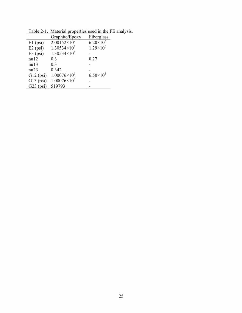
Table page 2-1 Material properties used in the FE analysis. ......................................................................25

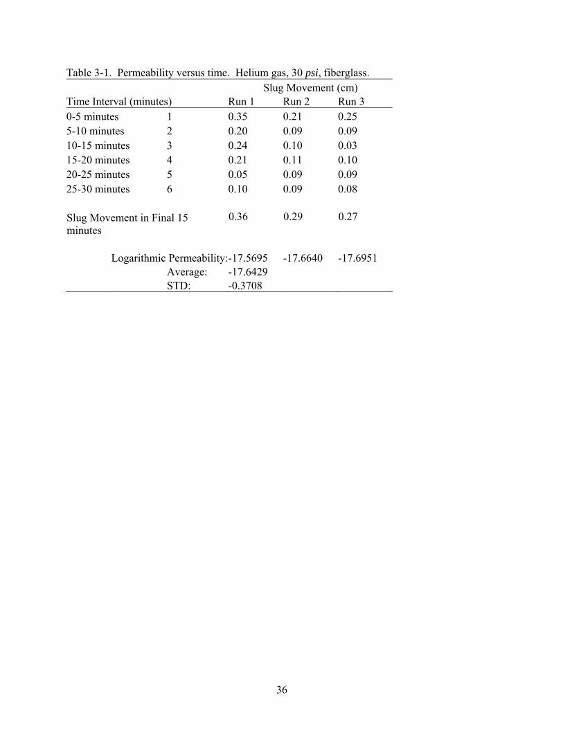
3-1 Permeability versus time. Helium gas, 30 psi, fiberglass. ................................................36

3-2 Permeability versus time. Nitrogen gas, 30 psi, fiberglass. ..............................................37

3-3 Permeability versus time. Helium gas, multiple upstream pressures, [0/0/90/90]s. .........38

3-4 Error used in uncertainty analysis......................................................................................38

8

LIST OF FIGURES

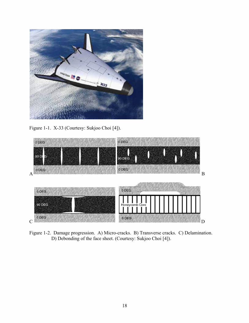
Figure page 1-1 X-33 (Courtesy: Sukjoo Choi [4]). ....................................................................................18

1-2 Damage progression. A) Micro-cracks. B) Transverse cracks. C) Delamination. D) Debonding of the face sheet. (Courtesy: Sukjoo Choi [4])................................................18

1-3 Volumetric permeability determination method (Courtesy: ASTM D1434-82 [10])........19

1-4 Permeability testing apparatus (Courtesy: Sukjoo Choi [4]). ............................................19

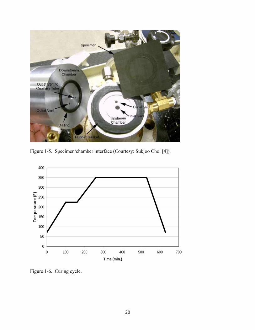
1-5 Specimen/chamber interface (Courtesy: Sukjoo Choi [4]). ...............................................20

1-6 Curing cycle. ......................................................................................................................20

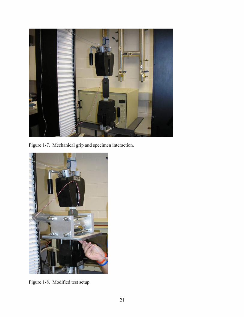
1-7 Mechanical grip and specimen interaction. .......................................................................21

1-8 Modified test setup.............................................................................................................21

2-1 Strain in the 2-direction of a [0/0/90/90]s specimen subjected to 100 pounds of tension. ...............................................................................................................................26

2-2 Stress in the 12-direction of a [0/0/90/90]s specimen subjected to 100 pounds of tension. ...............................................................................................................................27

2-3 Deflection of 0.001313 in. due to an upstream pressure of 10 psi.....................................28

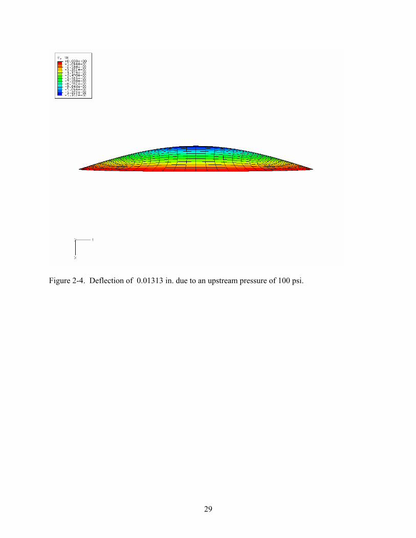
2-4 Deflection of 0.01313 in. due to an upstream pressure of 100 psi....................................29

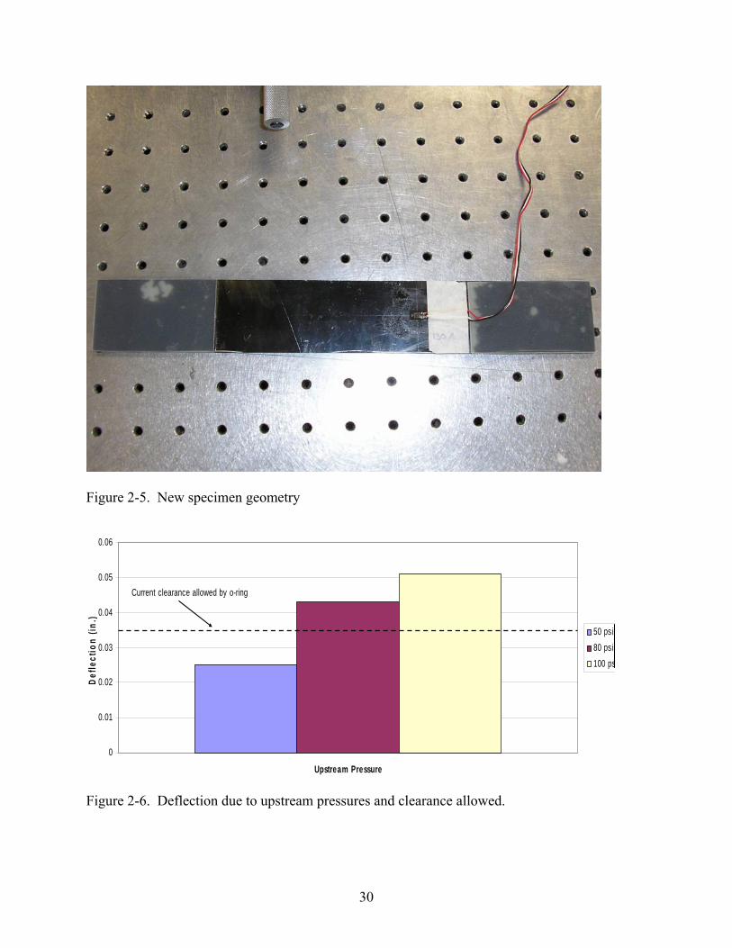
2-5 New specimen geometry....................................................................................................30

2-6 Deflection due to upstream pressures and clearance allowed............................................30

2-7 New geometry specimen deflection. A) Isometric view. B) Side view...........................31

3-1 Slug position versus time. Helium gas, 30 psi, fiberglass. ...............................................39

3-2 Permeability versus time. Helium gas, 30 psi, fiberglass. ................................................39

3-3 Slug position versus time. Nitrogen gas, 30 psi, fiberglass of thickness 0.5 mm.............39

3-4 Permeability versus time. Nitrogen gas, 30 psi, fiberglass. ..............................................40

3-5 Slug movement versus time interval. Helium gas, multiple pressures, [0/0/90/90]s........40

3-6 Permeability versus time interval. Helium gas, multiple pressures, [0/0/90/90]s. ...........41

9

3-7 Error bars associated with helium gas, 30 psi, and fiberglass. ..........................................41

4-1 Inverse dog bone specimen failure. ...................................................................................46

4-2 Failed inverse dog bone specimen. ....................................................................................46

4-3 Load versus strain curve for inverse dog bone specimen [0/90/0/90]s..............................47

4-4 Stress versus strain curve for inverse dog bone specimen [0/90/0/90]s. ...........................47

4-5 Failure on the front side of the specimen...........................................................................48

4-6 Failure on the back side of specimen. ................................................................................48

4-7 ε11 strain through the thickness from the FE analysis at 100 psi upstream pressure. ........49

4-8 ε11 strain through the thickness from the FE analysis at 50 psi upstream pressure. ..........49

4-9 ε11, ε22, and γ12 through the thickness from the laminate analysis program FALCO. Only axial load is assumed to act on the specimen. No upstream pressure is used..........50

4-10 Logarithmic permeability versus strain for [90/+θ/-θ/90] laminate...................................50

4-11 Logarithmic permeability versus time. 0.3389% strain, [90/+θ/-θ/90], 50 psi upstream pressure for specimen #144................................................................................51

4-12 Grip assembly for permeability versus strain measurements. ...........................................51

4-13 Side view of assembly for permeability versus strain measurements................................52

10

Abstract of Thesis Presented to the Graduate School of the University of Florida in Partial Fulfillment of the

Requirements for the Degree of Master of Science

EFFECT OF STRAIN ON THE GAS PERMEABILITY OF COMPOSITE LAMINATES

By

James VanPelt III

December 2006

Chair: Bhavani Sankar Cochair: Peter Ifju Major: Aerospace Engineering

Because of their excellent mechanical and thermal properties, fiber reinforced composite

materials are good candidates for various gas storage systems in space vehicles. However, micro-

cracking and delamination in these materials could lead to gas permeation and catastrophic

failure of the system. The purpose of this research is to investigate various factors including the

applied strains that affect the gas permeability. An experimental procedure has been developed

according to ASTM D1434-82 standards. In order to simulate the loads induced by launch and

landing of the vehicle, the composite specimens are subjected to a given load during the gas

permeation test.

Permeability values tended to converge after at least 15 minutes of test duration. Due to

higher molecular weight, Nitrogen permeated at a slower rate than Helium. Permeability did not

depend on upstream pressure when the specimens were not loaded. To test the permeability of

the specimens under load, the gas permeation test setup and the laminate were oriented in such a

manner that desired load could be applied to the specimen in the material testing machine. A

new geometry of specimen was developed such that there was a seamless integration between

machinery and specimens. Finite element modeling proved that the newly developed geometry

would allow for accurate permeability measurements. Finally, an uncertainty analysis was

11

performed to identify various sources of errors. The major source of error stemmed from length

measurements taken with calipers or rulers.

12

CHAPTER 1 INTRODUCTION

Composite Materials

Composites consist of two or more separate materials combined in a macroscopic

structural unit. They can be made from a combination of metals, polymers, or ceramics.

Structural composites made from polymers reinforced with fibers, such as glass and graphite,

have proven to be very effective. This is due to the fact that the composite materials are much

stronger and stiffer in fiber form than they are in bulk form. With a higher modulus and a lower

density, these fibers can lead to a great improvement in strength-to-weight ratio. Properties like

this have lead composites to be used greatly in the aerospace industry [1].

Aerospace Applications

The next generation of reusable launch vehicles (RLV) will require new and innovative

materials to reduce the cost of launching payloads into orbit from $10,000 per pound to $1,000.

One major issue of concern is using these fiber-reinforced composites to make durable,

lightweight, cryogenic propellant tanks. Various gas storage systems contribute to almost half

the dry weight of space vehicles. Using these materials in tank applications is very challenging

but promising in reducing the weight of future space vehicles [2].

X-33 Demonstrator: The sandwich liquid hydrogen (LH2) tank of the X-33

Demonstrator (Figure 1-1) was ground tested in 1999. When micro-cracking of the composite

inner skin occurred, the tank failed. Initially, the tank is filled with cryogenic fuels at extremely

low temperatures. This causes the material to shrink. Gas created by the evaporation of the LH2

caused the composite tank to rupture due to the micro-cracking associated with material

shrinkage [3]. There are also various stresses imposed on the tank when the vehicle is launched

and then during reentry and landing. Figure 1-2 [4] shows how the cryogenic fuel can leak

13

through micro-cracks induced by these stresses. When the micro-cracks develop, they provide a

pathway for the gas to leak through the specimen. The example in Figure 1-2 is a [0/90/0] layup.

The goal of this research is to measure how much gas permeates through specimens of various

orientations and understand various factors that affect the permeability measurements.

Literature Review/Previous Work on Permeability Testing

There have been many ongoing tests in the past investigating the permeability of various

materials in cryogenic storage applications. Some tests explored how the addition of polymer

films to the composite laminate would decrease the permeability of the testing material. Several

commercially available and LaRC films exhibited lower permeability than the composite panels

tested which would imply adding these films to the panels would lower the permeability of the

tank [2]. Other film research was performed with films that were preconditioned. This consisted

of combinations of elevated temperature, cryogenic temperature, and moisture for extended

periods of time. It was shown that the preconditioning of the films had no significant effect on

permeability. On of the films, Tedlar, possessed the best barrier properties, allowing the least

amount of He gas to permeate [5].

Permeability tests were also conducted on sandwich core materials containing a Hexcel

HRP or DuPont Korex core with graphite/epoxy facesheets. These panels were subjected to

static and dynamic shear loads. Permeability increased instantaneously when catastrophic failure

occurred (failure occurred at the bondline). Also, as the number of cycles increased during the

tests, permeability increased for the Korex core [6]. A tetra-axial test was also performed on a

Bismaleimide (BMI) based graphite fiber composite material. Permeability was seen to increase

right before catastrophic failure occurred. It was also found that due to creep, permeability s a

time dependent parameter [7].

14

The effect of impact testing and the permeability’s dependence on upstream pressure (post-

impact) has also been explored. For post-impact testing, the permeability has a non-linear

dependence on the upstream pressure. An increase in pressure results in a more substantial

increase in permeability. These tests were conducted using a bubble-type leak detector that

corresponded with the qualitative permeability measurements [8].

Combining cryogenic applications with tensile loading on carbon fiber laminates was also

the focus of previous research. Significant leakage was observed under liquid Nitrogen testing

conditions when a tensile load was applied. When compared to the leakage at room temperature

at the same tensile load, permeability only varied slightly. There remained some mechanical

effect of the cryogenic storage condition that affected the permeability of the material [9].

Standard Test Method for Determining Gas Permeability

In order to measure the amount of gas that permeates through a specimen, a volumetric

determination method was developed based on ASTM D1434 standards [10]. This method can

be seen in Figure 1-3. A specimen to be tested is placed in between an upstream and a

downstream chamber. The downstream chamber is open to atmospheric pressure. Any gas that

permeates through the specimen is indicated by a volume change in gas. This volume manifests

itself in the movement of a liquid slug downstream of the permeating gas.

Permeability Apparatus

The permeability apparatus used is shown in Figure 1-4. Gas enters from the tank through

the upstream gas inlet tube. The precision pressure regulator then adjusts the upstream pressure

of the gas entering the upstream chamber. Upstream pressure is measured with a P-303A

pressure transducer from Omega Engineering Inc. An outlet valve is located in the upstream

chamber to purge the system of any excess atmospheric gas before the test is conducted. Usually

the system was allowed to purge for five minutes before testing began. Gas then permeates

15

through the specimen when this outlet valve is closed. A close-up of this interaction is shown in

Figure 1-5. A greased gasket/O-ring interface is used as well as a 300-pound compressive force

so that no permeating gas might escape before entering the capillary tube.

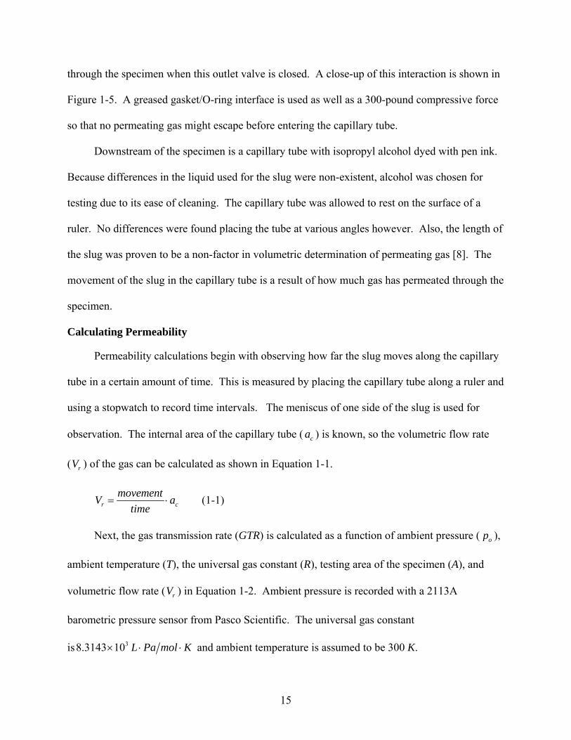
Downstream of the specimen is a capillary tube with isopropyl alcohol dyed with pen ink.

Because differences in the liquid used for the slug were non-existent, alcohol was chosen for

testing due to its ease of cleaning. The capillary tube was allowed to rest on the surface of a

ruler. No differences were found placing the tube at various angles however. Also, the length of

the slug was proven to be a non-factor in volumetric determination of permeating gas [8]. The

movement of the slug in the capillary tube is a result of how much gas has permeated through the

specimen.

Calculating Permeability

Permeability calculations begin with observing how far the slug moves along the capillary

tube in a certain amount of time. This is measured by placing the capillary tube along a ruler and

using a stopwatch to record time intervals. The meniscus of one side of the slug is used for

observation. The internal area of the capillary tube ( ca ) is known, so the volumetric flow rate

( rV ) of the gas can be calculated as shown in Equation 1-1.

r cmovementV a

time= ⋅ (1-1)

Next, the gas transmission rate (GTR) is calculated as a function of ambient pressure ( op ),

ambient temperature (T), the universal gas constant (R), testing area of the specimen (A), and

volumetric flow rate ( rV ) in Equation 1-2. Ambient pressure is recorded with a 2113A

barometric pressure sensor from Pasco Scientific. The universal gas constant

is 38.3143 10 L Pa mol K× ⋅ ⋅ and ambient temperature is assumed to be 300 K.

16

o rp VGTRA R T

⋅=

⋅ ⋅ (1-2)

The permeance (P), in Equation 1-3, is calculated by knowing the upstream pressure (p)

and GTR. Permeability ( P ) is the permeance multiplied with the thickness (t) of the specimen,

as shown in Equation 1-4.

o

GTRPp p

=−

(1-3)

P P t= ⋅ (1-4)

Units for permeability are mol/s/m/Pa. The logarithm of permeability is taken and will be

used in the rest of this document for greater ease in comparing results. It should be noted that the

logarithmic permeability is usually a negative number, and hence higher the magnitude (absolute

value) of the log of permeability, the less permeable the material is.

Testing Specimens

Various testing samples were fabricated using graphite/epoxy prepregs in an autoclave.

The layers were configured in specific orientations and then cured. Prepregs used for initial

samples were from Torayca and were product number T800HB-12K-40B. The curing cycle for

these specimens involved constant atmospheric pressure and a vacuum of -30 in. Hg. First, the

specimens were heated to 225°F and held for one hour. Then, they were raised to 350°F and

held for four and a half hours before returning to room temperature. This temperature

distribution is outlined in Figure 1-6.

Specimens were then cut in an inverse dog bone shape (Figure 1-7). This shape resulted

from the grip and testing area constraints. The specimen was required to be cut so that it could

be centered within the mechanical grips used for loading the specimen while being wide enough

17

in the body to accommodate the testing area of the gasket. Fiberglass tabs were adhered to the

tips with a hysol epoxy. It will be shown later why the specimen must fit into the grip.

Testing Adapted for Strain

To allow for permeability testing while the specimen is undergoing a load, the prior setup,

shown in Figure 1-4, had to be modified. Instead of using the MTI machine as a source for the

300 pounds of compressive force, it had to now be used to apply external load to the specimen.

In order to accomplish this, a bracket was designed to hold the upstream and downstream

chambers horizontally as shown in Figure 1-8. A torque wrench was used to tighten the brackets

around the specimen providing the clamping force required for no gas to escape.

Strain in the specimen was measured using a 120 Ω uniaxial Vishay Micro-Measurements

strain gage. Load was measured using a 25,000 pound load cell. The MTI machine is rated up

to 30,000 pounds and the grips’ capacity is 30,000 pounds. A LabVIEW program monitors load

versus strain for various testing situations. Permeability is still calculated as before. All data

sensors were monitored in the same fashion as previously explained.

18

Figure 1-1. X-33 (Courtesy: Sukjoo Choi [4]).

A B

C D

Figure 1-2. Damage progression. A) Micro-cracks. B) Transverse cracks. C) Delamination. D) Debonding of the face sheet. (Courtesy: Sukjoo Choi [4]).

19

Figure 1-3. Volumetric permeability determination method (Courtesy: ASTM D1434-82 [10]).

Figure 1-4. Permeability testing apparatus (Courtesy: Sukjoo Choi [4]).

20

Figure 1-5. Specimen/chamber interface (Courtesy: Sukjoo Choi [4]).

0

50

100

150

200

250

300

350

400

0 100 200 300 400 500 600 700

Time (min.)

Tem

pera

ture

(F)

Figure 1-6. Curing cycle.

21

Figure 1-7. Mechanical grip and specimen interaction.

Figure 1-8. Modified test setup.

22

CHAPTER 2 FINITE ELEMENT MODELING

Motivation for Modeling

Due to the unique geometry of the specimen used in this research, a finite element analysis

was performed to investigate any major stress concentrations that might affect permeability

results. The fillets of radii of about 10 mm were cut into the specimen so that available grips

could be used without reducing the testing width of the testing area. There was also the question

of where to place the strain gage if these fillets might cause some adverse stress gradients. Also,

the deflection of the specimen due to the upstream pressure was investigated. There was concern

that the deflection might be too much for the system to handle. All finite element modeling was

performed using the commercial software Abaqus with material properties outlined in Table 2-1.

Strain Gage Placement

Initially, the specimens used were inverse dog bone shaped. This gave rise to the question

of where a suitable location for the strain gage would be. The strain gage cannot be placed over

the center of the specimen where testing occurs because it would be difficult to attach wires to

the specimen. Furthermore, placing a strain gage at the center of the testing area would interfere

with the permeating gas through the specimen. A model of the entire specimen was made to

investigate regions of similar strain. In this case, the model was of a [0/0/90/90]s layup. In

Abaqus, linear/quadratic elements with four nodes per element and three degrees of freedom per

node were used. The resulting strain in the 2-direction from applying 100 pounds is shown in

Figure 2-1. The strain in the 2-direction was found to be the only significant value of strain

measured.

From this model, it was determined that the strain gage could be placed anywhere along

the centerline of the specimen. For ease of testing, the gage was placed about one inch below the

23

fiberglass tab. This location should provide an accurate representation of the strain measured

across the testing area of the specimen without any upstream pressure applied.

In order to increase the accuracy of the FE model, a quarter-sized model was analyzed

using the same type of elements noted previously. Significant stress concentrations appeared in

the corner as more shear stresses developed. This is shown in Figure 2-2. The stress

concentrations were localized enough to confirm the validity of the strain gage placement.

Test Area Deflection

When the [0/0/90/90]s specimen is subjected to an upstream pressure, it will undergo some

deflection. A circular plate of diameter equal to that of the O-ring was analyzed with finite

elements. The plate was assumed to be on pinned support around the edges. For this analysis, 3-

D shell elements were used. S4R elements with four degrees of freedom per node were

subjected to pressures ranging from 10 to 100 psi. Figures 2-3 and 2-4 show the deflection

dependence on upstream pressure. Based on the results, the deflection dependence on upstream

pressure is a linear relationship. For a clamped condition, the maximum deflection from Abaqus

was 0.003539 in. The deflection due to all ranges of upstream pressures was very small and was

regarded as negligible for having any permeability interference.

Exploring Alternative Specimen Geometries

When fabricating the specimens had to be completed cheaper and faster to suit the testing

constraints, a new geometry was explored. The inverse dog bone shape is influenced by two

parameters: the grip width and the testing area. Grip width cannot change, for these grips have

the strength required for pulling the specimen to large strain levels. Testing area, however, can

change. The testing area is the area created by the radius of the gasket. By substituting an O-

ring for the gasket, the cross sectional area of testing is reduced. This would get rid of the

24

inverse dog bone shape and allow rectangular strips to be easily fabricated with a shear. A

picture of the new specimen geometry is shown in Figure 2-5.

New specimens cut to this geometry were four and six layer laminates. Strain field across

the specimen is now assumed to be uniform because of the uniform loading and the rectangular

geometry of the new specimens. However, due to the smaller thickness, a new deflection

analysis was performed. The thought was that a less thick specimen would deflect more and

possibly cover up and obstruct the permeating gas pathway to the capillary tube.

Abaqus Modeling of Deflection on New Geometry: Downstream of the specimen, there

is an outlet pathway that the permeating gas follows to get to the capillary tube. The clearance

between an un-deformed specimen and this hole is 0.035 in. A finite element model, created

with eight node shell elements with six degrees of freedom per node, shows that the deformation

due to 80 and 100 psi exceeds the given clearance of 0.035 in. This is shown graphically in

Figure 2-6. All tests conducted with the new geometry were to not exceed 50 psi in order to

avoid the excessive deflection that would obstruct the permeability measurements.

Shown in Figure 2-7 is a four layer specimen subjected to a tensile load of 1000 pounds

and to 100 psi upstream pressure across the testing area. The conjecture here is that the

deformation causes the specimen to interact with the inside of the downstream chamber, causing

some possible blocking of the outlet to the capillary tube. Two solutions exist; to obtain a

thicker O-ring, or to use 50 psi as the upstream pressure for all tests with the new specimen.

Choosing 50 psi upstream pressure was the choice made for further studies.

25

Table 2-1. Material properties used in the FE analysis. Graphite/Epoxy FiberglassE1 (psi) 2.00152×107 6.20×106 E2 (psi) 1.30534×107 1.29×106 E3 (psi) 1.30534×106 - nu12 0.3 0.27 nu13 0.3 - nu23 0.342 - G12 (psi) 1.00076×106 6.50×105 G13 (psi) 1.00076×106 - G23 (psi) 519793 -

26

Figure 2-1. Strain in the 2-direction of a [0/0/90/90]s specimen subjected to 100 pounds of

tension.

27

Figure 2-2. Stress in the 12-direction of a [0/0/90/90]s specimen subjected to 100 pounds of

tension.

28

Figure 2-3. Deflection of 0.001313 in. due to an upstream pressure of 10 psi.

29

Figure 2-4. Deflection of 0.01313 in. due to an upstream pressure of 100 psi.

30

Figure 2-5. New specimen geometry

Figure 2-6. Deflection due to upstream pressures and clearance allowed.

0

0.01

0.02

0.03

0.04

0.05

0.06

Upstream Pressure

Def

lect

ion

(in.)

50 psi80 psi100 ps

Current clearance allowed by o-ring

31

A

B

Figure 2-7. New geometry specimen deflection. A) Isometric view. B) Side view.

32

CHAPTER 3 PERMEABILITY INVESTIGATION

Initial Permeability Testing Criteria

To begin the experimental permeability testing, the inverse dog bone shape and fiberglass

specimens were used to verify certain parameters that would be used later for the rectangular

specimens. Three investigations were performed at no strain level. A relationship between

permeability and time was established. Dependence of permeability on upstream pressure was

recorded. Finally, the impact of gas selection on permeability was explored. Before any test was

completed, a control was initiated. This control was an aluminum plate. The aluminum plate

was inserted in the permeability testing apparatus. No slug movement was noted. This verified

no leaks existed in the system and that all testing could proceed as planned.

Permeability and Time

An investigation of permeability and time was performed using a fiberglass specimen, the

same material used on the tabs. Tests were performed with both helium and nitrogen gas at an

upstream pressure of 30 psi. The idea was to see if permeability values leveled out at a certain

time after testing was initiated.

For helium gas, the tests were allowed to run for 30 minutes. The position of the slug was

recorded every five minutes. This gave six intervals of slug movement and thus six intervals of

permeability calculations. Table 3-1 shows the values obtained from this test. The highlighted

section of the table illustrates the intervals were permeability converged. Average permeability

and the standard deviation are dually noted. Figure 3-1 outlines the slug position versus time,

while Figure 3-2 shows the permeability versus time. Again, the logarithm of permeability is

taken for ease of comparison.

33

The same analysis was performed using Nitrogen as the permeating gas. Initially, the tests

were allowed to run for 30 minutes. One final test was allowed to run for 60 minutes because it

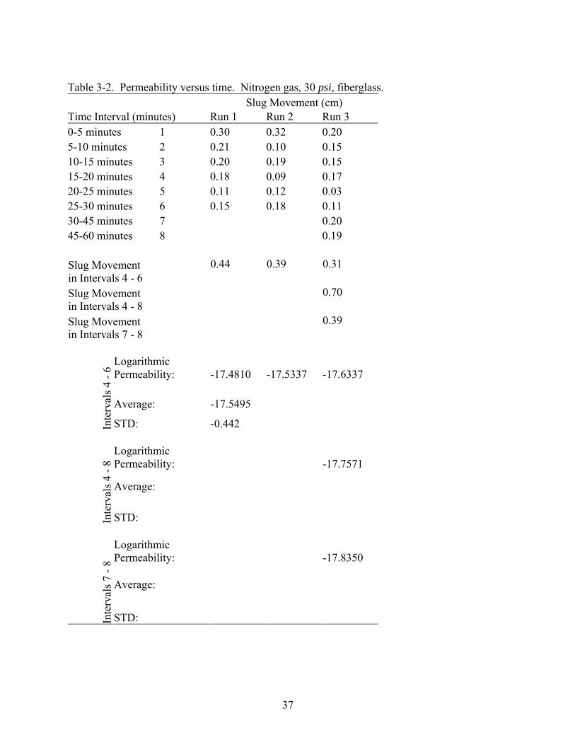
was expected that nitrogen would take longer to permeate due to its larger atomic size. Table 3-2

shows results from this test. Slug movement and permeability for this test began to converge

after 30 minutes of testing as shown in Figures 3-3 and 3-4.

The conclusion that can be made from this analysis is that the data obtained during the first

20 minutes of the testing duration should be disregarded. Gas was still turned on and slug

movement monitored, but only permeability values after 20 minutes were averaged together to

give results.

Permeability and Upstream Pressure

It has already been noted that using the inverse dog bone specimens is acceptable up to 100

psi. The next step was to determine if permeability depended on upstream pressure. The

precision pressure regulator would only allow up to 60 psi upstream pressure. So, tests were

performed at 10, 50, and 60 psi. The specimen used in this case was a [0/0/90/90]s inverse dog

bone shaped laminate. Helium gas was used in all cases and was allowed to permeate for 30

minutes. Based on the permeability versus time analysis performed, all permeability values are

the average over the final 15 minutes of the test.

It was found that in an unstrained condition, permeability does not depend on upstream

pressure. Figure 3-5 shows the slug movement versus time for the three upstream pressures.

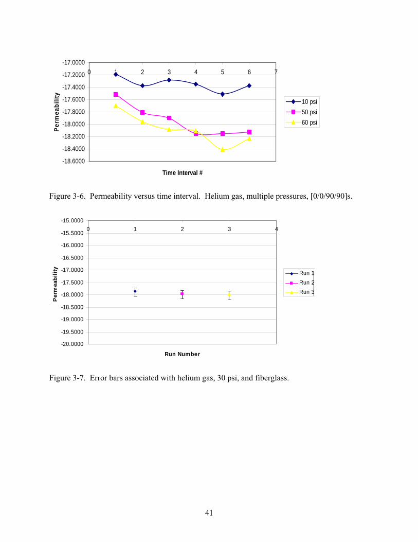
There is good convergence after the first 15 minutes. Figure 3-6 shows the permeability versus

time in each case. It appears at first glance that there is a large discrepancy in permeability data.

This difference is attributed to a slug movement differential of less than 0.5 mm. This data is

shown in Table 3-3. Such a small difference could be attributed to eye sight error in reading the

slug movement.

34

Based on the tested results, it is concluded that permeability does not depend on upstream

pressure in a non loaded case. For future testing with the dog bone shaped specimen, 30 psi was

selected as the upstream pressure. Rectangular specimens were tested at an upstream pressure of

50 psi. Both of these values are within the limits set by the FE modeling of deflection of a

circular disk.

Permeability and Gas Selection

The final analysis performed on the fiberglass specimens was on the relationship of

permeability and gas selection. Two gases were used in these tests: helium and nitrogen. Prior

to conducting the tests, the assumption was that permeability values should be lower for nitrogen

because it is a larger molecule than helium.

Helium values converged at a logarithmic permeability of -17.6429 from Table 3-1. From

Table 3-2, it can be seen that nitrogen values converge to -17.8350. Only permeability values

based on the permeability versus time analysis were used in averaging. The higher the

magnitude (absolute value) of the logarithmic permeability, the lower the permeability, or the

less gas that leaks through the specimen. This proves the initial theory that nitrogen permeates at

a slower rate than helium. Helium gas was used for the duration of testing.

Uncertainty Analysis

Due to the multiple readings that are made during these tests, an uncertainty analysis was

performed to investigate how each measurement affects the final calculation. The first step in

determining the uncertainty in each calculation was to first set up a general equation for

calculating the permeability of the material. Next, the derivative of the general equation was

taken with respect to each variable present in the equation. Once the derivatives were expressed

in terms of the measured variables, the error in each measurement was determined. Error was

35

associated with ruler readings, eye sight, and pressure sensors. In all cases, reasonable error (u)

was determined, as shown in Table 3-4.

The next step of the uncertainty analysis involves substituting the experimental values

obtained during the test into each derivative equation. This value of the derivative is noted as kd ,

where k is the respective variable from Table 3-4 for each case. Finally, Equation 3-1 illustrates

how the uncertainty (U) is obtained for the overall test.

2 2 2 2 2 2k k l l m mU d u d u d u= ⋅ + ⋅ + ⋅ +K (3-1)

Once the uncertainty value is calculated, it is added and subtracted to the initial

permeability value obtained from the test. Once this has been completed, the logarithm is taken.

The MATLAB code used in this method is shown in Appendix A. By analyzing each

2 2k kd u⋅ component of Equation 3-1, the affect of each measurement can be compared with each

other to determine the largest sources of error. The largest sources of error were observed to be

any readings made with a ruler. These included the distance the slug moves, the radius of the

capillary tube, the thickness of the specimen, and the radius of the testing area. Of particular

note is that the distance the slug moves contributes to a large source of error.

This supports the conclusion that the permeability does not depend on upstream pressure.

Differences in those measurements were less than one millimeter, which is difficult to observe

with the naked eye. However, even those small differences can contribute to large error in the

final results. Error bars were plotted according to this uncertainty method, as shown in Figure 3-

7.

36

Table 3-1. Permeability versus time. Helium gas, 30 psi, fiberglass. Slug Movement (cm) Time Interval (minutes) Run 1 Run 2 Run 3 0-5 minutes 1 0.35 0.21 0.25 5-10 minutes 2 0.20 0.09 0.09 10-15 minutes 3 0.24 0.10 0.03 15-20 minutes 4 0.21 0.11 0.10 20-25 minutes 5 0.05 0.09 0.09 25-30 minutes 6 0.10 0.09 0.08

0.36 0.29 0.27 Slug Movement in Final 15 minutes Logarithmic Permeability:-17.5695 -17.6640 -17.6951 Average: -17.6429 STD: -0.3708

37

Table 3-2. Permeability versus time. Nitrogen gas, 30 psi, fiberglass. Slug Movement (cm) Time Interval (minutes) Run 1 Run 2 Run 3 0-5 minutes 1 0.30 0.32 0.20 5-10 minutes 2 0.21 0.10 0.15 10-15 minutes 3 0.20 0.19 0.15 15-20 minutes 4 0.18 0.09 0.17 20-25 minutes 5 0.11 0.12 0.03 25-30 minutes 6 0.15 0.18 0.11 30-45 minutes 7 0.20 45-60 minutes 8 0.19

0.44 0.39 0.31 Slug Movement in Intervals 4 - 6

0.70 Slug Movement in Intervals 4 - 8

0.39 Slug Movement in Intervals 7 - 8

Logarithmic Permeability: -17.4810 -17.5337 -17.6337

Average: -17.5495

Inte

rval

s 4 -

6

STD: -0.442

Logarithmic Permeability: -17.7571

Average:

Inte

rval

s 4 -

8

STD:

Logarithmic Permeability: -17.8350

Average:

Inte

rval

s 7 -

8

STD:

38

Table 3-3. Permeability versus time. Helium gas, multiple upstream pressures, [0/0/90/90]s. Slug Movement (cm) Time Interval (minutes) 10 psi 50 psi 60 psi 0-5 minutes 1 0.27 0.65 0.51 5-10 minutes 2 0.18 0.33 0.28 10-15 minutes 3 0.22 0.27 0.21 15-20 minutes 4 0.19 0.15 0.20 20-25 minutes 5 0.13 0.15 0.10 25-30 minutes 6 0.18 0.16 0.15

0.50 0.46 0.45 Slug Movement in Final 15 minutes Logarithmic Permeability:-17.4033 -18.1411 -18.2300 Average: -17.9248 STD: -2.5318 Table 3-4. Error used in uncertainty analysis. Variable Quantity Measured value SI Unit Po Ambient Pressure 16.932 Pa dslug Distance Slug Moves 0.0005 m rc Capillary Tube Radius 0.0000127 m P Upstream Pressure 9.191 Pa t Thickness 0.0005 m Rt Testing Area Radius 0.000794 m R Universal Gas Constant N/A N/A T Temperature N/A N/A time Time of Test 1 s

39

19.00

19.50

20.00

20.50

21.00

21.50

22.00

0 5 10 15 20 25 30 35

Time (minutes)

Posi

tion

(cm

)

Run 1

Run 2

Run 3

Figure 3-1. Slug position versus time. Helium gas, 30 psi, fiberglass.

-18.4000

-18.2000

-18.0000

-17.8000

-17.6000

-17.4000

-17.2000

-17.00000 1 2 3 4 5 6 7

Time Interval #

Perm

eabi

lity

Run 1Run 2Run 3

Figure 3-2. Permeability versus time. Helium gas, 30 psi, fiberglass.

0.00

5.00

10.00

15.00

20.00

25.00

0 10 20 30 40 50 60 70

Time (minutes)

Posi

tion

(cm

)

Run 1

Run 2

Run 3

Figure 3-3. Slug position versus time. Nitrogen gas, 30 psi, fiberglass of thickness 0.5 mm.

40

-18.4000

-18.2000

-18.0000

-17.8000

-17.6000

-17.4000

-17.2000

-17.00000 2 4 6 8 10

Time Interval #

Perm

eabi

lity

Run 1Run 2Run 3

Figure 3-4. Permeability versus time. Nitrogen gas, 30 psi, fiberglass.

0.00

0.10

0.20

0.30

0.40

0.50

0.60

0.70

0 1 2 3 4 5 6 7

Time Interval #

Slug

Mov

emen

t (cm

)

10 psi50 psi60 psi

Figure 3-5. Slug movement versus time interval. Helium gas, multiple pressures, [0/0/90/90]s.

41

-18.6000

-18.4000

-18.2000

-18.0000

-17.8000

-17.6000

-17.4000

-17.2000

-17.00000 1 2 3 4 5 6 7

Time Interval #

Perm

eabi

lity

10 psi50 psi60 psi

Figure 3-6. Permeability versus time interval. Helium gas, multiple pressures, [0/0/90/90]s.

Figure 3-7. Error bars associated with helium gas, 30 psi, and fiberglass.

-20.0000

-19.5000

-19.0000

-18.5000

-18.0000

-17.5000

-17.0000

-16.5000

-16.0000

-15.5000

-15.00000 1 2 3 4

Run Number

Per

mea

bilit

y

Run 1Run 2Run 3

42

CHAPTER 4 STRENGTH TESTING

Grouping the Specimens

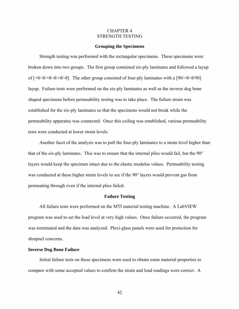
Strength testing was performed with the rectangular specimens. These specimens were

broken down into two groups. The first group contained six-ply laminates and followed a layup

of [+θ/-θ/+θ/-θ/+θ/-θ]. The other group consisted of four-ply laminates with a [90/+θ/-θ/90]

layup. Failure tests were performed on the six-ply laminates as well as the inverse dog bone

shaped specimens before permeability testing was to take place. The failure strain was

established for the six-ply laminates so that the specimens would not break while the

permeability apparatus was connected. Once this ceiling was established, various permeability

tests were conducted at lower strain levels.

Another facet of the analysis was to pull the four-ply laminates to a strain level higher than

that of the six-ply laminates. This was to ensure that the internal plies would fail, but the 90°

layers would keep the specimen intact due to the elastic modulus values. Permeability testing

was conducted at these higher strain levels to see if the 90° layers would prevent gas from

permeating through even if the internal plies failed.

Failure Testing

All failure tests were performed on the MTI material testing machine. A LabVIEW

program was used to set the load level at very high values. Once failure occurred, the program

was terminated and the data was analyzed. Plexi-glass panels were used for protection for

shrapnel concerns.

Inverse Dog Bone Failure

Initial failure tests on these specimens were used to obtain some material properties to

compare with some accepted values to confirm the strain and load readings were correct. A

43

[0/90/0/90]s specimen was used for the failure test. Once failure occurred, shown in Figures 4-1

and 4-2, the data was tabulated from the LabVIEW program. This program outputs load versus

strain. Knowing the cross-sectional area of the specimen allowed for a stress versus strain plot.

The slope of this line, the modulus of elasticity, was compared to accepted values. These plots

are shown in Figures 4-3 and 4-4.

A modulus of elasticity value from the stress versus strain curve was calculated to be 7.99

Msi. Accepted values for similar materials are E1 = 19.0 Msi and E2 = 1.5 Msi [1]. Due to a

layup of [0/90/0/90]s, the specimen was expected to have a modulus somewhere in between

those values. This procedure confirmed that the load cell and strain gage were working as

planned.

Rectangular Strip Failure

Failure tests on these specimens were conducted on the six-ply laminates. Due to the

layup consisting of [+θ/-θ/+θ/-θ/+θ/-θ], it was expected that these specimens would fail quite

early on in the loading process. There were six of these six-ply specimens to be tested. Of the

six, two had inherent flaws in them that prevented them from being tested. Of the remaining

four, two failed simply when the grips were attached to the specimen. With two specimens

remaining, one was taken to failure to learn the strain ceiling that could be placed on such a

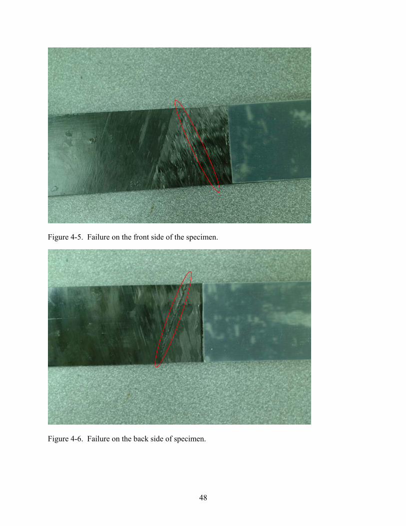
laminate. This specimen failed at 0.37% strain. Figures 4-5 and 4-6 illustrate the type of failure

that occurred along the ply angle. It was assumed then that taking the last laminate to a strain

level of 0.33% would be ok. This worked fine until an upstream pressure of helium gas was

applied to the specimen. When this happened, the specimen failed across the testing area due to

the deflection caused by the upstream pressure.

No permeability tests were able to be completed on these six-ply laminates for the reasons

stated above. However, the useful information taken out of them was two fold: the internal ply

44

failure strain of the four-ply laminates, and the idea that the specimen undergoes a strain increase

over the testing area that cannot be detected by the strain gage. An analysis of this strain level

had to be conducted.

Strain Through the Thickness

In a four-ply laminate, when the specimen is pulled to 1000 pounds and an upstream

pressure of 100 psi is applied, the strain gage reads 0.2537% strain. With an upstream pressure

of 100 psi, there must be a large deformation across the testing area and an associated strain with

it. Using Abaqus FE software, the strain in each layer was able to be extracted across the testing

area by picking a node within this area to analyze. The model in Figure 2-7 was used for this

analysis. A node close to where the strain gage was placed was also analyzed. This would

confirm that the FE model was in fact giving results comparable to the experimental results. For

the 100 psi case, Figure 4-7 shows the strain in each layer with the coordinate along the fiber

axis.

The strain gage readings were confirmed with the FE model; both were close to 0.25%

strain. However, the strain reading through the testing area was larger. Thus, the strain gage

readings only tell part of the story. However, if we only use 50 psi upstream pressure, the

difference between the two readings is much smaller as shown in Figure 4-8. This is another

reason why 50 psi was selected for the upstream pressure during the permeability tests.

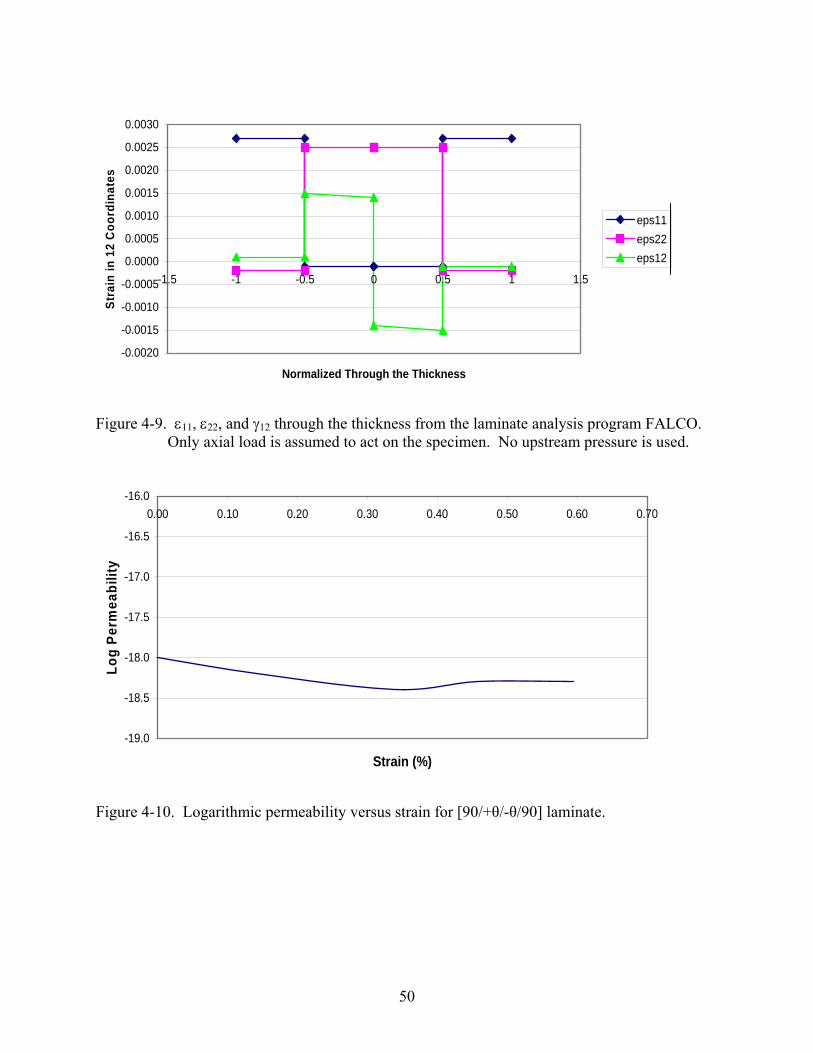
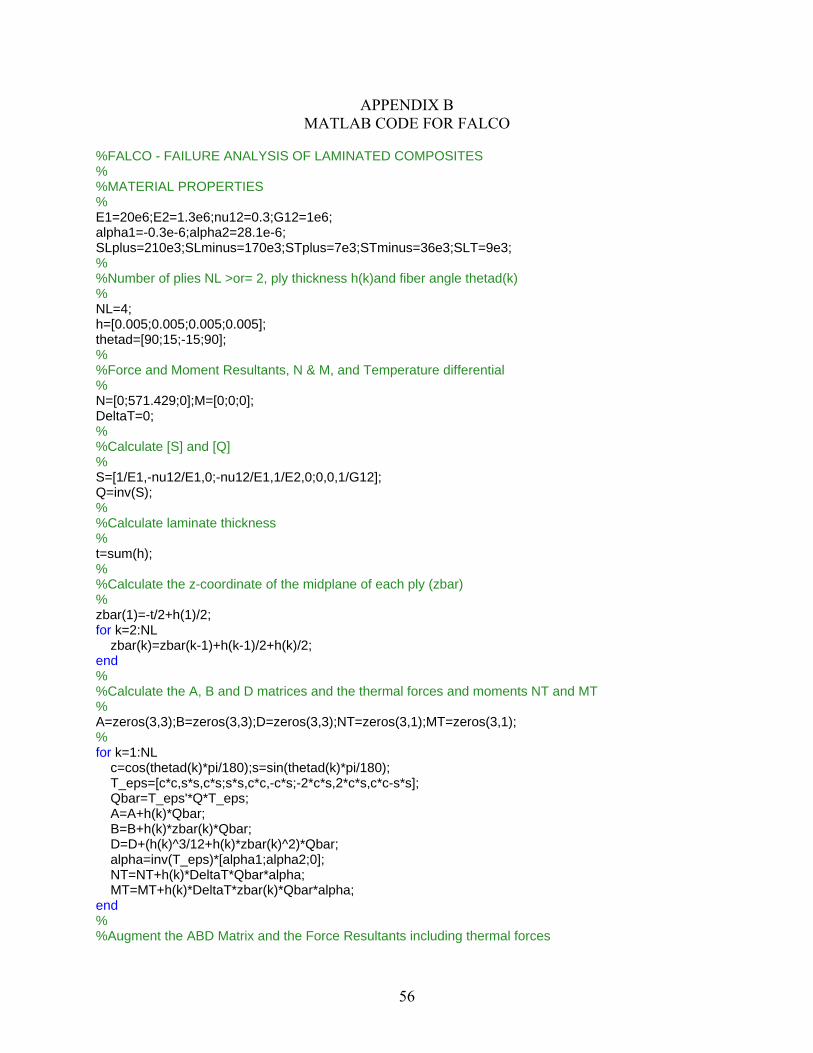
A further investigation was completed using a Failure Analysis of Laminated Composites

(FALCO). The MATLAB code for FALCO is included in Appendix B. In Figure 4-9, the

strains through the thickness were analyzed. As with the FE model, the experimental strain

reading of 0.2537% strain matches up very closely with computer-generated results. With

FALCO though, the upstream pressure cannot be taken into consideration.

45

Permeability and Strain

The goal of these tests is to find at which strain level the permeability increases by an order

of magnitude. Strips of [90/+θ/-θ/90] laminates were subjected to strain levels beyond the failure

strain of the internal [+θ/-θ] plies. First, a test was completed without any external strain. Then,

the LabVIEW program would be configured to pull the specimen to a desired load and hold it

there for 200 minutes. This would give plenty of time to configure the permeability apparatus

around the specimen and conduct a 100 minute test. Then the specimen would be unloaded and

loaded to a load 500 pounds greater and the test would be repeated.

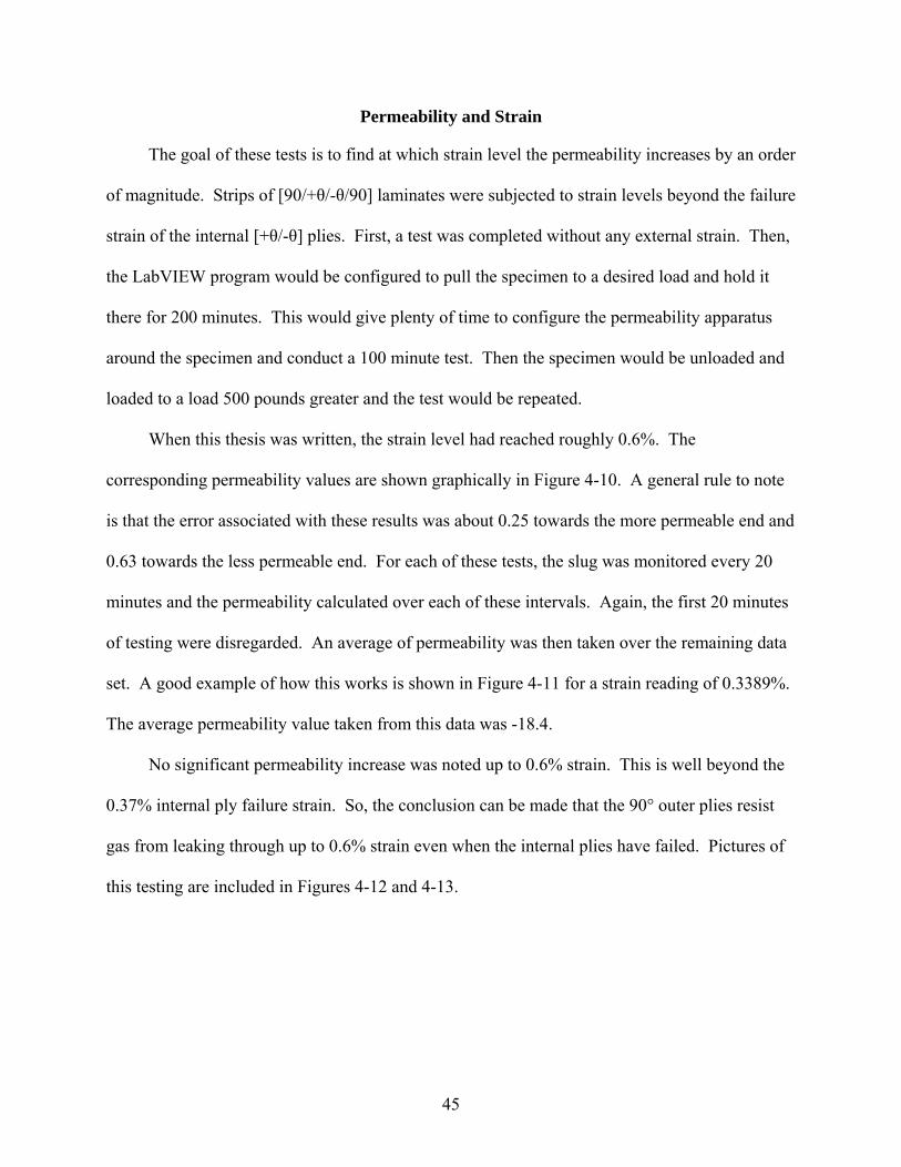
When this thesis was written, the strain level had reached roughly 0.6%. The

corresponding permeability values are shown graphically in Figure 4-10. A general rule to note

is that the error associated with these results was about 0.25 towards the more permeable end and

0.63 towards the less permeable end. For each of these tests, the slug was monitored every 20

minutes and the permeability calculated over each of these intervals. Again, the first 20 minutes

of testing were disregarded. An average of permeability was then taken over the remaining data

set. A good example of how this works is shown in Figure 4-11 for a strain reading of 0.3389%.

The average permeability value taken from this data was -18.4.

No significant permeability increase was noted up to 0.6% strain. This is well beyond the

0.37% internal ply failure strain. So, the conclusion can be made that the 90° outer plies resist

gas from leaking through up to 0.6% strain even when the internal plies have failed. Pictures of

this testing are included in Figures 4-12 and 4-13.

46

Figure 4-1. Inverse dog bone specimen failure.

Figure 4-2. Failed inverse dog bone specimen.

47

0.000

1000.000

2000.000

3000.000

4000.000

5000.000

6000.000

7000.000

8000.000

0 1000 2000 3000 4000 5000 6000 7000 8000 9000 10000

Microstrain

Load

(lbs

.)

Specimen failed at 0.905195 % strain and 6,751.058 lbs.

FAILURE

Figure 4-3. Load versus strain curve for inverse dog bone specimen [0/90/0/90]s.

0.00

10000.00

20000.00

30000.00

40000.00

50000.00

60000.00

70000.00

80000.00

0 1000 2000 3000 4000 5000 6000 7000 8000 9000 10000

Microstrain

Stre

ss (p

si.)

Specimen failed at 0.905195 % strain and 71,854.93 psiModulus of Elasticity from failure = 7.99 Msi

FAILURE

Figure 4-4. Stress versus strain curve for inverse dog bone specimen [0/90/0/90]s.

48

Figure 4-5. Failure on the front side of the specimen.

Figure 4-6. Failure on the back side of specimen.

49

-0.004

-0.002

0.000

0.002

0.004

0.006

0.008

-1.50 -1.00 -0.50 0.00 0.50 1.00 1.50

Through the Thickness

Stra

in (E

11)

In Testing AreaStrain Gage Location

Figure 4-7. ε11 strain through the thickness from the FE analysis at 100 psi upstream pressure.

-0.004

-0.002

0.000

0.002

0.004

0.006

0.008

-1.50 -1.00 -0.50 0.00 0.50 1.00 1.50

Through the Thickness

Stra

in (E

11)

In Testing AreaStrain Gage Location

Figure 4-8. ε11 strain through the thickness from the FE analysis at 50 psi upstream pressure.

50

-0.0020

-0.0015

-0.0010

-0.0005

0.0000

0.0005

0.0010

0.0015

0.0020

0.0025

0.0030

-1.5 -1 -0.5 0 0.5 1 1.5

Normalized Through the Thickness

Stra

in in

12

Coo

rdin

ates

eps11eps22eps12

Figure 4-9. ε11, ε22, and γ12 through the thickness from the laminate analysis program FALCO. Only axial load is assumed to act on the specimen. No upstream pressure is used.

-19.0

-18.5

-18.0

-17.5

-17.0

-16.5

-16.00.00 0.10 0.20 0.30 0.40 0.50 0.60 0.70

Strain (%)

Log

Perm

eabi

lity

Figure 4-10. Logarithmic permeability versus strain for [90/+θ/-θ/90] laminate.

51

-19.4

-19.2

-19

-18.8

-18.6

-18.4

-18.2

-18

-17.8

-17.6

-17.40 1 2 3 4 5 6

Interval Number

Log

Perm

eabi

lity

Figure 4-11. Logarithmic permeability versus time. 0.3389% strain, [90/+θ/-θ/90], 50 psi upstream pressure for specimen #144.

Figure 4-12. Grip assembly for permeability versus strain measurements.

52

Figure 4-13. Side view of assembly for permeability versus strain measurements.

53

CHAPTER 5 CONCLUSIONS AND FUTURE WORK

Due to the micro-cracking associated with various strain levels during launch and landing,

the permeability of gas through graphite/epoxy laminates is a major area of concern for reusable

launch vehicles and future space vehicles. An effective method for testing the permeability of

graphite/epoxy composite laminates under load was developed. This testing method allows for

permeability values to be determined at various strain levels.

Finite element modeling was instrumental in exploring other specimen geometries and in

establishing criteria for testing standards. Permeability was found to level out after 20 minutes

of testing. Prior to any micro-cracking developments, permeability did not depend on upstream

pressure. In addition, permeability was lower for nitrogen compared to helium. Thus, testing

with helium takes shorter time than nitrogen tests. A standard test evolved which included

testing with helium gas at an upstream pressure of 50 psi. An uncertainty analysis was

performed to investigate the contributions of the testing devices to the overall error in the system.

Finally, permeability was found to remain relatively constant up to 0.6% strain for the

four-layer laminates. This is past the point where the internal plies of the laminate fail. Up to

this strain level, the 90° layers prevent gas from leaking through. Future work from here would

involve combining the cryogenic environment with the strain level. An insulated casing of some

type could be placed around the already developed testing apparatus to conduct the permeability

tests at cryogenic temperatures.

54

APPENDIX A MATLAB CODE FOR PERMEABILITY

%%%%% Program for computing the permeability of composite laminates %%%%% %%%%% Created by Jim VanPelt %%%%% %%% USER INPUTS %%% Amb_press_Hg = 30.223; %%% Ambient pressure read by PASPORT sensor in inches Mercury Upstream_press_psi = 50; %%% Upstream pressure measured by Labview software "single.vi" time_min = 20; %%% Time permeability test is allowed to run in minutes distance_mm = 5.0; %%% Distance slug moved in millimeters thickness_in = .026; %%% Thickness of specimen in inches %%% CONVERSION %%% radius_cap_m = 0.000525; %%% Radius of Capillary Tube in meters radius_test_m = 0.0159; %%% Radius of testing area in meters Amb_press_Pa = 3386.388666667 * Amb_press_Hg; %%% Converts pressure from inches mercury to Pascals time_sec = 60 * time_min; %%% Converts time from minutes to seconds distance_m = distance_mm / 1000; %%% Converts distance slug moved from millimeters to meters Upstream_press_Pa = 6894.75728 * Upstream_press_psi; %%% Converts upstream pressure from psi to Pascals thickness_m = 0.0254 * thickness_in; %%% Converts thickness from inches to meters %%% PROPERTIES OF TESTING APPARATUS %%% Area_cap = pi*radius_cap_m^2; %%% Cross sectional area of capillary tube in m^2 Area_test = pi*radius_test_m^2; %%% Cross sectional testing area in m^2 To = 300; %%% Ambient temperature in Kelvin R = 8.3143e3; %%% Universal gas constant in (L*Pa)/(mol*K) %%% VOLUMETRIC FLOW RATE %%% slope = distance_m / time_sec; %%% Rate at which slug moves in m/s Vr = slope * Area_cap; %%% Volumetric flow rate in m^3/s %%% GAS TRANSMISSION RATE %%% GTR = (Amb_press_Pa * Vr) / (Area_test * R * To); %%% Gas transmission rate calculation %%% PERMEANCE %%% P = GTR / (Upstream_press_Pa - Amb_press_Pa); %%% Calculates permeance of specimen %%% PERMEABILITY %%% Perm = P * thickness_m; %%% Calculates permeability of specimen %%% LOG OF PERMEABILITY %%% P_bar = log10(Perm); %%% Calculates log of permeability for easier quantification %%%%% Uncertainty Analysis %%%%% %%% Displacements %%% u_Amb_press_Pa = 16.932; %%% Uncertainty in Ambient Pressure measurements

55

u_distance_m = 0.0005; %%% Uncertainty in Slug measurements u_radius_cap_m = 0.0000127; %%% Uncertainty in Capillary Tube Radius measurement u_Upstream_press_Pa = 9.191; %%% Uncertainty in Upstream pressure measurements u_thickness_m = 0.0005; %%% Uncertainty in thickness of specimen measurement u_radius_test_m = 0.000794; %%% Uncertainty in testing area radius u_time_s = 1; %%% Uncertainty in time measurements %%% Derivatives %%% dP_bar_dAmb_press = (distance_m * radius_cap_m^2 * Upstream_press_Pa * thickness_m) / ((Amb_press_Pa - Upstream_press_Pa)^2 * radius_test_m^2 * R * To * time_sec); dP_bar_ddslug = (-Amb_press_Pa * radius_cap_m^2 * thickness_m) / ((Amb_press_Pa - Upstream_press_Pa) * radius_test_m^2 * R * To * time_sec); dP_bar_dradius_cap = (-2 * radius_cap_m * Amb_press_Pa * distance_m * thickness_m) / ((Amb_press_Pa - Upstream_press_Pa) * radius_test_m^2 * R * To * time_sec); dP_bar_dupstream_press = (-Amb_press_Pa * distance_m * radius_cap_m^2 * thickness_m) / ((Upstream_press_Pa - Amb_press_Pa)^2 * radius_test_m^2 * R * To * time_sec); dP_bar_dthickness = (-Amb_press_Pa * distance_m * radius_cap_m^2) / ((Amb_press_Pa - Upstream_press_Pa) * radius_test_m^2 * R * To * time_sec); dP_bar_dradius_test = (2 * Amb_press_Pa * distance_m * radius_cap_m^2 * thickness_m) / (radius_test_m^3 * (Amb_press_Pa - Upstream_press_Pa) * R * To * time_sec); dP_bar_dtime = (Amb_press_Pa * distance_m * radius_cap_m^2 * thickness_m) / (time_sec^2 * (Amb_press_Pa - Upstream_press_Pa) * radius_test_m^2 * R * To); %%% Calculating the overall uncertainty %%% U = ((dP_bar_dAmb_press^2 * u_Amb_press_Pa^2) + (dP_bar_ddslug^2 * u_distance_m^2) + (dP_bar_dradius_cap^2 * u_radius_cap_m^2) + (dP_bar_dupstream_press^2 * u_Upstream_press_Pa^2) + (dP_bar_dthickness^2 * u_thickness_m^2) + (dP_bar_dradius_test^2 * u_radius_test_m^2) + (dP_bar_dtime^2 * u_time_s^2))^0.5; Perm_Upper = Perm + U; Perm_Lower = Perm - U; P_bar_Upper = log10(Perm_Upper); P_bar_Lower = log10(Perm_Lower); Difference_Upper = P_bar_Upper - P_bar; Difference_Lower = P_bar - P_bar_Lower; P_bar_Upper Difference_Upper P_bar Difference_Lower P_bar_Lower % Contribution_Ambient_Pressure = (dP_bar_dAmb_press^2 * u_Amb_press_Pa^2) % Contribution_Slug_Movement = (dP_bar_ddslug^2 * u_distance_m^2) % Contribution_Capillary_Radius = (dP_bar_dradius_cap^2 * u_radius_cap_m^2) % Contribution_Upstream_Pressure = (dP_bar_dupstream_press^2 * u_Upstream_press_Pa^2) % Contribution_Specimen_Thickness = (dP_bar_dthickness^2 * u_thickness_m^2) % Contribution_Test_Radius = (dP_bar_dradius_test^2 * u_radius_test_m^2) % Contribution_Time = (dP_bar_dtime^2 * u_time_s^2) % % Total = Contribution_Ambient_Pressure+Contribution_Slug_Movement+Contribution_Capillary_Radius+Contribution_Upstream_Pressure+Contribution_Specimen_Thickness+Contribution_Test_Radius+Contribution_Time % SquareRoot = Total^0.5

56

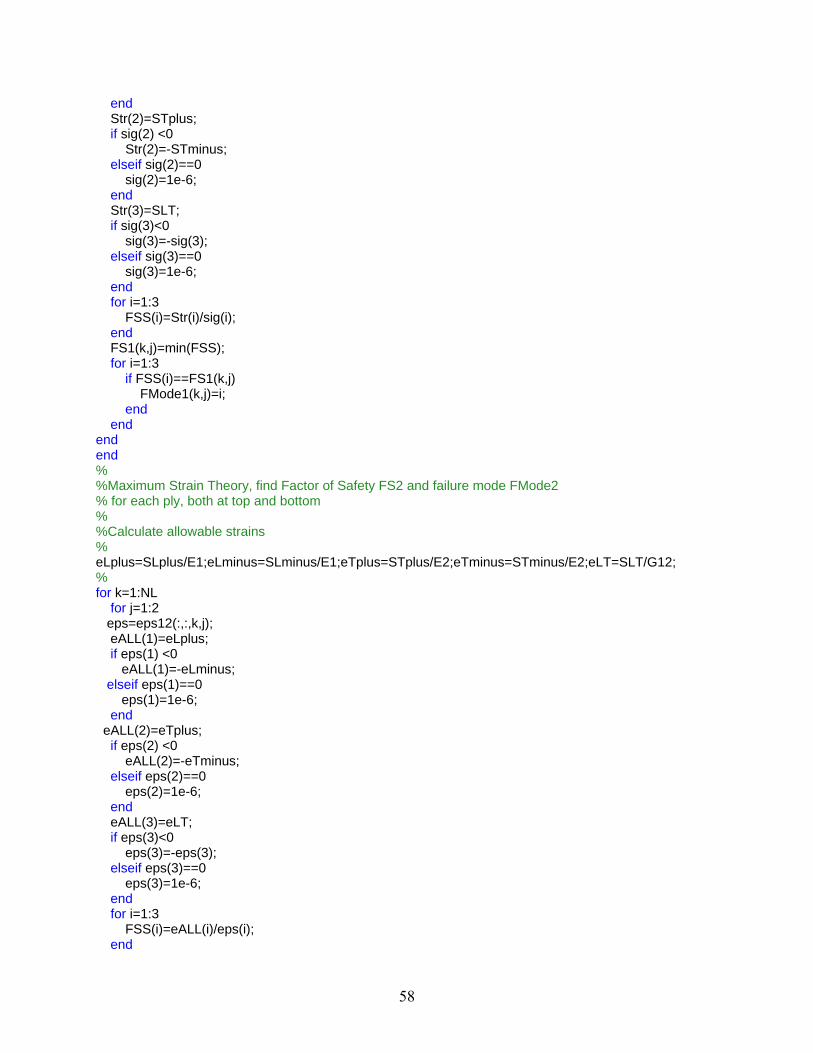
APPENDIX B MATLAB CODE FOR FALCO

%FALCO - FAILURE ANALYSIS OF LAMINATED COMPOSITES % %MATERIAL PROPERTIES % E1=20e6;E2=1.3e6;nu12=0.3;G12=1e6; alpha1=-0.3e-6;alpha2=28.1e-6; SLplus=210e3;SLminus=170e3;STplus=7e3;STminus=36e3;SLT=9e3; % %Number of plies NL >or= 2, ply thickness h(k)and fiber angle thetad(k) % NL=4; h=[0.005;0.005;0.005;0.005]; thetad=[90;15;-15;90]; % %Force and Moment Resultants, N & M, and Temperature differential % N=[0;571.429;0];M=[0;0;0]; DeltaT=0; % %Calculate [S] and [Q] % S=[1/E1,-nu12/E1,0;-nu12/E1,1/E2,0;0,0,1/G12]; Q=inv(S); % %Calculate laminate thickness % t=sum(h); % %Calculate the z-coordinate of the midplane of each ply (zbar) % zbar(1)=-t/2+h(1)/2; for k=2:NL zbar(k)=zbar(k-1)+h(k-1)/2+h(k)/2; end % %Calculate the A, B and D matrices and the thermal forces and moments NT and MT % A=zeros(3,3);B=zeros(3,3);D=zeros(3,3);NT=zeros(3,1);MT=zeros(3,1); % for k=1:NL c=cos(thetad(k)*pi/180);s=sin(thetad(k)*pi/180); T_eps=[c*c,s*s,c*s;s*s,c*c,-c*s;-2*c*s,2*c*s,c*c-s*s]; Qbar=T_eps'*Q*T_eps; A=A+h(k)*Qbar; B=B+h(k)*zbar(k)*Qbar; D=D+(h(k)^3/12+h(k)*zbar(k)^2)*Qbar; alpha=inv(T_eps)*[alpha1;alpha2;0]; NT=NT+h(k)*DeltaT*Qbar*alpha; MT=MT+h(k)*DeltaT*zbar(k)*Qbar*alpha; end % %Augment the ABD Matrix and the Force Resultants including thermal forces

57

% ABD=[A,B;B,D]; F=[N+NT;M+MT]; % %Compute the laminate deformations, %midplane strains eps0 and curvatures kappa % def=inv(ABD)*F; eps0=[def(1);def(2);def(3)];kappa=[def(4);def(5);def(6)]; % %determine the strains and stresses in each ply %Strains and Stresses are calculated at the top and bottom surfaces of each ply %strains and stresses are in respective principal material coordinates % eps12=zeros(3,1,NL,2);sig12=zeros(3,1,NL,2); % for k=1:NL c=cos(thetad(k)*pi/180);s=sin(thetad(k)*pi/180); T_eps=[c*c,s*s,c*s;s*s,c*c,-c*s;-2*c*s,2*c*s,c*c-s*s]; epsxy=eps0+(zbar(k)+h(k)/2)*kappa; sigxy=T_eps'*Q*T_eps*epsxy; % %Calculate the strains and stresses at the top of the ply % eps12(:,:,k,1)=T_eps*epsxy; sig12(:,:,k,1)=Q*(eps12(:,:,k,1)-DeltaT*[alpha1;alpha2;0]); % %Calculate the strains and stresses at the bottom of the ply % epsxy=eps0+(zbar(k)-h(k)/2)*kappa; eps12(:,:,k,2)=T_eps*epsxy; sig12(:,:,k,2)=Q*eps12(:,:,k,2); end % %Factor of Safety (FS) is determined for each ply at bottom and top surfaces %Factor of Safety according to Max Stress Theory is FS1 %Factor of safety According to Max strain theory is FS2 %Factor of Safety according to Tsai-Hill is FS3 %Factor of safety according to Tsai-Wu is FS4 % %Similarly failure mode FMode1, FMode2 etc are calculated %FMode=1 means fiber failure, 2 indicates transverse failure and 3 Shear failure % FS1=zeros(NL,2);FS2=zeros(NL,2);FS3=zeros(NL,2);FS4=zeros(NL,2); % %Maximum Stress Theory, find Factor of Safety FS1 and failure mode FMode1 % for each ply, both at top and bottom % for k=1:NL for j=1:2 sig=sig12(:,:,k,j); Str(1)=SLplus; if sig(1) <0 Str(1)=-SLminus; elseif sig(1)==0 sig(1)=1e-6;

58

end Str(2)=STplus; if sig(2) <0 Str(2)=-STminus; elseif sig(2)==0 sig(2)=1e-6; end Str(3)=SLT; if sig(3)<0 sig(3)=-sig(3); elseif sig(3)==0 sig(3)=1e-6; end for i=1:3 FSS(i)=Str(i)/sig(i); end FS1(k,j)=min(FSS); for i=1:3 if FSS(i)==FS1(k,j) FMode1(k,j)=i; end end end end % %Maximum Strain Theory, find Factor of Safety FS2 and failure mode FMode2 % for each ply, both at top and bottom % %Calculate allowable strains % eLplus=SLplus/E1;eLminus=SLminus/E1;eTplus=STplus/E2;eTminus=STminus/E2;eLT=SLT/G12; % for k=1:NL for j=1:2 eps=eps12(:,:,k,j); eALL(1)=eLplus; if eps(1) <0 eALL(1)=-eLminus; elseif eps(1)==0 eps(1)=1e-6; end eALL(2)=eTplus; if eps(2) <0 eALL(2)=-eTminus; elseif eps(2)==0 eps(2)=1e-6; end eALL(3)=eLT; if eps(3)<0 eps(3)=-eps(3); elseif eps(3)==0 eps(3)=1e-6; end for i=1:3 FSS(i)=eALL(i)/eps(i); end

59

FS2(k,j)=min(FSS); for i=1:3 if FSS(i)==FS2(k,j) FMode2(k,j)=i; end end end end % %Tsai-Hill Theory FS3, Note that Failure Mode is determined based on Max. Stress Theory % i.e., FMode3=FMode1 % for k=1:NL for j=1:2 sig=sig12(:,:,k,j); Str(1)=SLplus; if sig(1) <0 Str(1)=-SLminus; end Str(2)=STplus; if sig(2) <0 Str(2)=-STminus; end Str(3)=SLT; FS3(k,j)=1/sqrt((sig(1)/Str(1))^2-sig(1)*sig(2)/Str(1)^2+(sig(2)/Str(2))^2+(sig(3)/Str(3))^2); FMode3(k,j)=FMode1(k,j); end end % %Tsai-Wu Theory FS4, Note that Failure Mode is determined based on Max. Stress Theory % i.e., FMode4=FMode1 % %Compute Tsai_Wu coefficients F11, F1, F22 etc. % F11=1/(SLplus*SLminus);F1=1/SLplus-1/SLminus;F22=1/(STplus*STminus);F2=1/STplus-1/STminus; F66=1/SLT^2;F12=-sqrt(F11*F22)/2; % for k=1:NL for j=1:2 sig=sig12(:,:,k,j); FS4(k,j)=1/(F11*sig(1)^2+F22*sig(2)^2+F66*sig(3)^2+F1*sig(1)+F2*sig(2)+2*F12*sig(1)*sig(2)); FMode4(k,j)=FMode1(k,j); end end

60

LIST OF REFERENCES

1. Gibson, Ronald F. (1994). Principles of Composite Material Mechanics. New York: McGraw-Hill Companies, Inc. 2. Grimsley, B., Cano, R., Johnston, N., Loos, A. and McMahon, W., “Hybrid Composites for LH2 Fuel Tank structure,” Proceedings of the 33rd International SAMPE Technical Conference, NASA Langley Research Center, November 4-8, 2001.

3. NASA, Final Report of the X-33 Liquid Hydrogen Tank Test Investigation Team, George C. Marshall Space Flight Center, Huntsville, 2000, May. 4. Choi, Sukjoo. “Micromechanics, Fracture Mechanics and Gas Permeability of Composite Laminates for Cryogenic Storage Systems.” University of Florida, 2006. 5. Herring, H. M., “Characterization of Thin Film Polymers Through Dynamic Mechanical Analysis and Permeation,” NASA CR 212422, June 2003. 6. Glass, D. E., Raman, V.V., Venkat, V. S., and Sankaran, S. N., “Honeycomb Core Permeability Under Mechanical Loads,” NASA CR 206263, December 1997. 7. Stokes, E. H., “Hydrogen Permeability of Polymer Based Composite Tank Material Under Tetra-Axial Strain,” Proceedings of the 5th Conference on Aerospace Materials, Processes, and Environmental Technology (AMPET), Huntsville, AL, September 16-18, 2002. 8. Nettles, A.T., “Permeability Testing of Impacted Composite Laminates for Use on Reusable Launch Vehicles,” NASA/TM-2001-210799, 2001. 9. Yokozeki, T., Aoki, T., and Ishikawa, T., “Gas Permeability of Microcracked Laminates Under Cryogenic Conditions,” Proceedings of the 44th AIAA/ASME/ASCE/AHS Structures, Structural Dynamics, and Materials Conference, Norfolk, VA, April 7-10, 2003. 10. ASTM D1434-82 (Reapproved 1992), “Standard Test Method for Determining Gas permeability Characteristics of Plastic Film and Sheeting,” ASTM, 203-213, 1992.

61

BIOGRAPHICAL SKETCH

James VanPelt III (Jim) was born on August 17, 1982 in Bloomfield, NJ. He spent much

of his young childhood moving from New Jersey to Pennsylvania to Virginia before finally

settling back in West Chester, PA prior to the second grade. Jim later graduated in May of 2000

from West Chester East High School about 30 minutes west of Philadelphia. Some of his

activities included playing the viola in district and regional state orchestras, golfing on the high

school team, playing travel soccer, becoming proficient in horseback riding, and achieving Star

in Boy Scouts.

In the summer of 2000, Jim began undergraduate studies at the University of Florida in

Aerospace Engineering. He joined the social fraternity Beta Theta Pi which would be the source

of many fond memories in his undergraduate life. Some of his other activities included helping

to found the Small Satellite Design Club and being an active member of the American Institute

of Aeronautics and Astronautics. After graduating from the University of Florida in April 2005,

Jim began graduate school under the tutelage of Dr. Bhavani V. Sankar in the Department of

Mechanical and Aerospace Engineering. It was here that his interest in composites began to

grow as he conducted permeability experiments on graphite/epoxy laminates. He graduated with

a Master of Science in aerospace engineering from the University of Florida in December 2006.

Jim is the son of James VanPelt II and Daphne Faye Hager. He has a younger brother,

Quinn Hager, and a younger sister, Holly Hager, whom he loves very much. After graduating,

Jim will work on space systems for Lockheed Martin in New Orleans, LA.