Effect of Objective Function on the Optimization of Highway Vertical ...€¦ · the vertical...

Civil Engineering Infrastructures Journal, 53(1): 115– 136, June 2020

Print ISSN: 2322-2093; Online ISSN: 2423-6691

DOI: 10.22059/ceij.2019.279837.1578

* Corresponding author E-mail: [email protected]

115

Effect of Objective Function on the Optimization of Highway Vertical

Alignment by Means of Metaheuristic Algorithms

Ghanizadeh, A.R.1*, Heidarabadizadeh, N.2 and Mahmoodabadi, M.J.3

1 Associate Professor, Department of Civil Engineering, Sirjan University of Technology,

Sirjan, Iran. 2 Research Assistant, Department of Civil Engineering, Sirjan University of Technology,

Sirjan, Iran. 3 Associate Professor, Department of Mechanical Engineering, Sirjan University of

Technology, Sirjan, Iran.

Received: 25 Apr. 2019; Revised: 01 Aug. 2019; Accepted: 17 Aug. 2019

ABSTRACT: The main purpose of this work is the comparison of several objective

functions for optimization of the vertical alignment. To this end, after formulation of

optimum vertical alignment problem based on different constraints, the objective function

was considered as four forms including: 1) the sum of the absolute value of variance between

the vertical alignment and the existing ground; 2) the sum of the absolute value of variance

between the vertical alignment and the existing ground based on the diverse weights for cuts

and fills; 3) the sum of cut and fill volumes; and 4) the earthwork cost and then the value of

objective function was compared for the first three cases with the last one, which was the

most accurate ones. In order to optimize the raised problem, Genetic Algorithm (GA) and

Group Search Optimization (GSO) were implemented and performance of these two

optimization algorithms were also compared. This research proves that the minimization of

sum of the absolute value of variance between the vertical alignment and the existing ground,

which is commonly used for design of vertical alignment, can’t at all grantee the optimum

vertical alignment in terms of earthwork cost.

Keywords: Earthwork Volumes, Group Search Optimization (GSO), Objective Function,

Optimization, Optimum Vertical Alignment.

INTRODUCTION

There are three key stages for designing

highways including designing the horizontal

alignment, designing vertical alignment, and

calculating the earthwork volumes. In fact, in

the initial stage, the location or horizontal

alignment of the highway is designed based

on the topographic maps and the maximum

allowable grade, and in the second stage the

vertical alignment or project should be

designed according to the design criteria and

minimizing construction costs. In the third

step, considering the typical cross section, the

cross sections along the highway were printed

and the fill and cut volumes are estimated.

After designing the horizontal alignment,

the most effective parameter on the highway

construction costs is the optimum design of

the vertical alignment for decreasing the

Ghanizadeh, A.R. et al.

116

earthwork volumes. Moreover, the correct

design of the vertical alignment is very

effective on the safety and cost of the

vehicles. Some works emphasized that the

vertical alignment should be designed as

close as possible to the existing ground line

(Garber and Hoel, 2014; Abbey, 1992;

AUSTROADS, 1993; Papacostas and

Prevedouros, 1993; Banks, 2002). In contrast,

some references highlight other factors like

earthwork minimization and achieving cut-

fill balance, to design the vertical alignment

(AASHTO, 2011; CALTRANS, 1995).

Enhancing the vertical alignment

minimizes the total value of the earthwork

costs. To decrease the highway construction

costs, a systematic approach should be

implemented to choose the optimal vertical

alignment. Besides minimizing earthwork

costs, some restrictions like the maximum

and minimum grade of tangents, minimum

length of vertical curves, minimum height of

bridges, and non-overlapping of vertical

curves should be evaluated to design the

vertical alignment.

Until now, numerous researches have

attempted to optimize the vertical alignment

for highway and railway routes. In Table 1,

some of these researches and their main

characteristics have been represented.

As shown, since calculation of earthwork

volume is complicated, in the majority of

previous researches, the sum of the absolute

value of variance between the vertical

alignment and the existing ground has been

considered as objective function to tackle the

problem of optimum vertical alignment.

Moreover, in some other researches which

have considered the earthwork volume as the

objective function, this volume has been

obtained by using approximate approaches

and hence, the exact volume of the earthwork

has not been considered in most of previous

works. So, one of the main purpose of the

present research is optimizing vertical

alignment based on the accurate estimation of

earthwork volumes.

In this work, the comparison of different

objective functions for optimization of

vertical alignment is investigated. The

objective function is considered as four forms

including: 1) the sum of the absolute value of

variance between the vertical alignment and

the existing ground; 2) the sum of the

absolute value of variance between the

vertical alignment and the existing ground

based on the diverse weights for cuts and fills;

3) the sum of cut and fill volumes; and 4) the

earthwork cost.

The main purpose of vertical alignment

design is decreasing the earthwork cost;

therefore, the fourth objective function is the

most appropriate one (Fwa et al., 2002;

CALTRANS, 1995; AASHTO, 2011).

Although minimizing the earthwork cost is

the most appropriate objective function for

designing the vertical alignment, but due to

the complexity, minimizing the difference

between the vertical alignment and the

ground line at the road centerline is usually

used for the manual design of the vertical

alignment.

On the other hand, run time for estimation

of earthwork cost is much higher than

estimation of difference between the vertical

alignment and ground line at the road

centerline, which makes it almost impossible

to use this function for routine design of

vertical alignment. So in this research, to

evaluate other objective functions, the

optimum vertical alignment is achieved first

by other three objective functions and then,

their results will be compared with that of the

optimum vertical alignment according to the

earthwork cost. Besides, a comparison was

conducted between the performance of two

different optimization algorithms including

Genetic Algorithm (GA) and Group Search

Optimization (GSO) in terms of the problem

of vertical alignment optimization.

Civil Engineering Infrastructures Journal, 53(1): 115 – 136, June 2020

117

Table 1. A summary of researches conducted on optimizing the vertical alignment

Reference Objective function Constraint Method

(Easa, 1988) Minimization of earthmoving The slop of the tangent Linear programming

(Easa, 1999)

The sum of the absolute deviations

between the observed profile and the

vertical curve

- Linear programming

(Dabbour et al.,

2002)

The sum of difference between

vertical alignment and existing

ground profile

Maximum allowable grade,

maximum vertical curvature

and non-overlapping of

vertical curves

Nonlinear

programming

(Göktepe et al.,

2008)

Using Fuzzy system to determine

swell and shrinkage factor - Fuzzy method

(Göktepe et al.,

2009)

The sum of squared differences

between calculated weighted ground

elevations and grade elevations

Maximum allowable gradient

and sight distance

Fuzzy method and

genetic algorithm

(Göktepe et al.,

2010)

The sum of differences between

calculated weighted ground

elevations and grade elevations


and sight distance

Dynamic

programming

(Wang et al.,

2011)


vertical alignment and ground profile

in the center line of the road

Maximum allowable gradient,

vertical curvature constraint

and sight distance

Genetic algorithm

(Bababeik and

Monajjem,

2012)

Total construction and operating

costs Maximum allowable grade

Direct search

method and genetic

algorithm

(Rahman, 2012) Total excavation, embankment, and

hauling cost Natural blocks and side slopes

Mixed integer linear

programming

(Mil and

Piantanakulchai,

2013)



in the center line


and minimum vertical curve

length

Polynomial

regression model

(Li et al., 2013)

Total earth work, land acquisition,

bridges, tunnels, retaining structure

and length-related costs

Maximum allowable gradient,

vertical curvature and

minimum curvature radius

Dynamic

Programming

(Kazemi and

Shafahi, 2013)

The sum of construction costs and

earthwork costs

Maximum grade and

minimum length of vertical

curves

Parallel processing

and PSO algorithm

(Shafahi and

Bagherian,

2013)

Total right-of-way and earthwork

costs

Minimum radius, maximum

and minimum length for

vertical curves

PSO algorithm

(Tunahoglu and

Soycan, 2014)



in the center line of the road

Maximum and minimum

allowable grades Searching algorithm

(Hare et al.,

2014) Minimization of earthmoving

Side slopes and physical

blocks in the terrain

mixed-integer linear

programming and

quasi-network flow

(Al-Sobky,

2014)

The earthwork balance and equal cut

and fill quantities

Minimum grade of tangents,

minimum length of vertical

curves

Linear programming

(Hare et al.,

2015)

The minimization of the total

excavation cost, embankment cost

and hauling cost.

Side-slopes of the road and

the natural blocks

mixed-integer linear

programming

(Beiranvand et

al. 2017)

The minimization of the total

excavation cost and embankment cost

The borrow and waste pit and

the natural blocks

Multi-haul quasi

network flow model

(Ghanizadeh

and

heidarabadizade

h, 2018)

minimization of Earthwork cost

Maximum and minimum

grade of tangents, minimum

length of vertical curves,

compulsory points

colliding bodies

optimization

algorithm


118

OPTIMIZATION ALGORITHMS

Genetic Algorithm

So far, various metaheuristic optimization

algorithms have been developed and

employed successfully in the field of civil

infrastructure engineering (Shafahi and

Bagherian, 2013; Moosavian and Jaefarzade,

2015; Hadiwardoyo et al., 2017; Ghanizadeh

and Heydarabadizadeh, 2018; Husseinzadeh

Kashan et al., 2018). Genetic algorithm (GA)

is one of the first and most important of these

algorithms. Holland (1975) presented GA

with the inspiration of Darwin’s theory about

the survival of fittest. One of the capabilities

of stochastic algorithms is to work over a set

of solutions called population. Each member

of the population is called a chromosome

�⃗�𝑖 = [𝑥1, 𝑥2, … , 𝑥𝐷] where 𝐷: is the number

of gens. The standard version of the GA is

organized by three operators including

reproduction, crossover, and mutation. After

applying these operators, the new population

would be created. This process is iterated

until the stopping criterion is met, and the

chromosome with the best fitness would be

introduced as the optimal solution. The

details of the reproduction, crossover, and

mutation operators are described in the

following.

Reproduction: In a simple way, two

members of the population are selected

randomly then the member with less fitness is

removed from the population and the one

with more fitness is put in place. This

operator is done for (Pr × N) members of the

population. Where, Pr and N are the

probability of the reproduction and the size of

the population, respectively.

Crossover: A crossover operator selects

two members of the population randomly.

Then, it creates two new chromosomes and

puts them at the place of the old

chromosomes. The crossover operator is

usually applied to a number of pairs

determined as (Ptc × N)/2, where Ptc and N:

are the probability of the crossover and the

population size, respectively. Let �⃗�𝑖(𝑡) and

�⃗�𝑗(𝑡) be two randomly selected

chromosomes and �⃗�𝑖(𝑡) has the smaller

fitness value than �⃗�𝑗(𝑡), then the crossover

relations are as follows.

(t))X- (t) X( +(t) X = 1)+(tX ji1i i

(t))X- (t) X( +(t) X = 1)+(tX ji2j j

(1)

where �⃗�1 and γ⃗⃗2∈ [0, 1]D: are random

vectors.

Mutation: Mutation operator causes

variations on the values of a number of

chromosomes in the population (determined

as Pm × N, where Pm and N: are the probability

of the mutation and the population size,

respectively). Let �⃗�𝑖(𝑡) a randomly selected

chromosome, and then the mutation

formulation is defined as:

b+(t) X = 1)+(tX ii

(2)

where �⃗⃗� ∈ [0, 1]𝐷: is a random vector and η

is a constant value (Mahmoodabadi and

Nemati, 2016).

Group Search Optimization

The Group Search Optimization algorithm

(GSO) inspired by animal behavior was

suggested by He et al. (He et al., 2006, 2009).

GSO uses the Producer-Scrounger model

(PS) as a framework. The PS model is based

on the social foraging strategies of groups

living animal. 1) Producing (searching for

food); and 2) Joining (joining resources

discovered by others) are two nutritional

strategies in the group. Basically, GSO is a

population-based optimization algorithm. In

GSO algorithm, the population is called the

group, and each individual in the population

is called a member. In an n-dimensional

search space, the ith member in the kth search

space has a current position nk

i RX and a


119

head angle 111

nk

)n(iki

ki R,..., and a head

direction 1,...,k k k k n

i i i inD d d R is defined

by the following equation:

1

11

n

p

kip

ki

cosd (3)

1

1

n

ip

kip

k)j(i

kij cos.sind (4)

k)n(i

kin sind

1 (5)

In the GSO algorithm, a group is consist of

three types of members: producer, scroungers

and rangers. Producer and scroungers

behavior is based on the PS model, but

rangers are used with random behavior to

avoid entrapment at the local minimum. In

the GSO algorithm, for accuracy and

convenience in calculations, only one

producer is considered in each replication,

and the rest of the remaining members are

assumed to be scroungers and ranger type.

During each iteration, a member of the group

is placed in the most satisfactory region and

obtains the best value of the target function,

which this member is considered as the

producer, and then the scroungers search

environment (optimal amount) is examined.

The scanning can be done through physical

contact, visual, chemical or auditory

mechanisms. The visual scanning is the main

mechanism for scan by many species of

animals, where is used by the producer in the

GSO. In optimization problems of more than

three dimensions, the visual scan is extended

to a n-dimensional space, which is

determined by the maximum pursuit angle 1 n

max R and the maximum pursuit distance

1Rlmax in the three-dimensional space.

These parameters are shown in Figure 1.

In the GSO algorithm, the kth iteration of

the behavior of the producer Xp will be as

follows:

1. The producer will scan zero degree and

then randomly scan three points in space,

which are:

one point at zero degree:

kkpmax

kpz DlrXX 1 (6)

A point on the right of the hypercube:

221 /rDlrXX maxkk

pmaxkpr (7)

A point on the left of the hypercube:

221 /rDlrXX maxkk

pmaxkpl (8)

where 1

1 Rr : is a random number with a

normal distribution with the mean of 0 and

the standard deviation of 1 and 1

2 nRr is the

random sequence in the range (0, 1).

Fig. 1. Scanning field in 3D space


120

2. Then the producer will find the best point

and the best resource. If the best point had a

better resource than its current position, it

flies toward that source. Otherwise, it stays in

its current position and moves to a new angle:

maxkk r 2

1 (9)

where max : is the maximum turning angle.

3. If the producer can’t find a better area after

an iteration, then it returns to zero degree:

kak

(10)

where a: is a constant that is obtained by

round 1n .

In each iteration, some of the members of

the group are selected as scrounger. In the kth

iteration, the behavior of the ith scrounger, can

be modeled as a random walk towards the

producer:

ki

kp

ki

ki XXrXX

31

(11)

where nRr 3 : is a uniform random sequence

in the range (0, 1).

In the GSO algorithm, random walks,

which is one of the most efficient way to

search for sources with random distribution,

is used by rangers. If the ith member of the

group is chosen as a ranger, in kth repeating,

this ranger produces a random angle and a

random distance li accordance to the

following relations:

max21 rk

iki

(12)

max1. lrali (13)

and moves to a new position using the

following equation (He et al., 2006).

11 kkii

ki

ki DlXX (14)

FORMULATION OF VERTICAL

ALIGNMENT OPTIMIZATION

Figure 2 represent the typical highway

longitudinal profile. In this figure, the

existing ground has been shown by dashed

line and vertical alignment with some PVIs

has been drawn up by solid line. The ith PVI

is identified by iPVIx ,

iPVIy and

iPVIL where

these parameters indicate the station,

elevation and vertical curve length, in the

respective order. The value of iPVIL for i = 1

and i = n was regarded zero.

Furthermore, station, elevation and

minimum allowable height of ith compulsory

point are depicted as i

Brgx , i

Brgy andi

Brgh ,

respectively.

Objective Function

In this research, four different objective

functions have been utilized for optimization

of vertical alignment. Table 2 presents the

considered objective functions used in this

work.

Table 2. The considered Objective functions in this research

Objective function Unit Formulation

The sum of the absolute value of difference between the

vertical alignment and the existing ground (m)

n

1i

i

FG

i

EG yy1F

The sum of the absolute value of difference between the

vertical alignment and the existing ground with respect to

different weights for cuts and fills

($/m2)

fc n

1j

j

EG

j

FG

n

1i

i

FG

i

EG yyyy2F

The sum of cut and fill volumes m3 fc VV3F

Total Earthwork cost ($) ff2cc1 VCVC4F


121

Fig. 2. A part of the longitudinal profile for a road

In Table 4, F1 to F4 are the objective

functions; i

EGy : is the height of the existing

ground for ith point, i

FGy : is the height of the

vertical alignment (finished ground) for ith

point, n: is the number of existing ground

points; α and β: are weights for cutting and

filling, respectively; nc: is the number of

existing ground points located in the cut; nf :

shows the number of existing ground points

located in the fill; δ1: denotes the swelling

factor; δ2: denotes the shrinkage factor; Cc:

denotes the cutting cost per m3; Cf : denotes

the filling cost per m3; Vc : denotes the cutting

volumes in m3, and Vf : denotes filling

volumes in m3.

To determine the Earthwork volume, it is

necessary to calculate the fill and cut areas for

two successive sections first; and then, the

prismoidal formula is used to calculate the

Earthwork volume. In this research, the

developed program uses the coordinate

method to calculate the fill and cut areas for

each section. Following the calculation of fill

and cut areas, the Earthwork volume between

two successive sections can be calculated by

applying the presmoidal approach. The

prismoidal formulation for computation of

cut or fill volumes is as follows:

L3

AAAAV

2121

(15)

where V: shows the volume between two

successive sections; A1: represents the area of

the first section; A2: represents the area of the

second section, and L: denotes the horizontal

distance between two successive sections. As

shown in Figure 3, the fill and cut volumes

between two consecutive sections is

calculated according to the fill and cut

conditions for two successive sections.

Constraints

Grade of Tangents

The topography of land, highway

category, the traction power of heavy

vehicles, safety, construction costs, drainage

considerations, and landscape liniment are

different parameters that dictate the

maximum and minimum grade of tangents in

vertical alignment (IMPO, 2012; AASHTO,

2011).

The grade of tangents should not surpass

the minimum and maximum allowable values

as the following:

i 1 ii PVI PVI

min maxi 1 iPVI PVI

y yg g g ; i 1,2,..., N 1

x x

(16)


122

Case 1 Case 2 Case 3

c

fffff

V

LAAAA

V

L3

AAAAV

0V

2c

1c

2c

1c

c

f

LAA

AL

LAA

AL

L3

AV

L3

AV

fc

f2

fc

c1

1c

c

2f

f

Case 4 Case 5 Case 6

LAAAA

V

LA

V

ccccc

ff

LAAAA

V

LAAAA

V

ccccc

fffff

LAA

AL

LAA

AL

LAA

AL

LAA

AL

3

LA

3

LAV

3

LA

3

LAV

2c

1f

2c

4

2c

1f

1f

3

2f

1c

2f

2

2f

1c

1c

1

42c1

1c

c

22f3

1f

f

Fig. 3. Computation of fill and cut volumes in terms of fill and cut conditions

Minimum Length of the Vertical Curves

Changing of the longitudinal grade is

gradually performed using the vertical

curves. Actually, the vertical curve must

fulfill the acceptable sight distance, drainage

of surface water, safety, driver comfort and

visual aesthetic of the highway. Normally, the

minimum sight distance for safe driving is

used to calculate the minimum acceptable

length of vertical curves (IMPO, 2012;

AASHTO, 2011). The minimum acceptable

length of the vertical curve should satisfy the

following relation:

i iL k A ; i 2,3,..., N 1 (17)

i 1 i i i 1PVI PVI PVI PVI

i i 1 i i i 1PVI PVI PVI PVI

y y y yA ;i 2,3,..., N 1

x x x x

(18)

where N: shows the number of vertical

alignment PVIs, Li: shows the length of the

vertical curve at ith PVI, Ai: denotes the

absolute variance between intersecting

tangent grades at ith PVI and k: shows the

curvature value of the vertical curve for one

percent of the grade difference. Other


123

parameters are illustrated in Figure 2. The

value of k is dependent on the design speed

and the type of the vertical curve (sag or

crest). Table 3 gives the k values for design of

vertical curves based on stopping sight

distance.

Table 3. k values for design of vertical curves

(IMPO, 2012)

k for sag

curve k for crest

curve Design speed

(Km/h)

13

18

23

30

38

45 55

63

73

7

11

17

26

39 52

74 95

124

50

60

70

80

90

100

110

120

130

Non-Overlapping of Two Successive

Vertical Curves

In order to increase the safety and comfort,

the final length of vertical curves is fixed to a

value more than the minimum acceptable

length. It is possible to increase the length of

vertical curves to the extent that the overlap

between two consequent vertical curves is

eliminated to keep the vertical alignment

continuous. Henceforth, the optimum vertical

alignment should meet the following

equation.

i 1 i

i 1 i PVI PVIPVI PVI

L Lx x ; i 2,3,..., N 2

2

(19)

where i

PVIx and i

PVIL : show the station and

vertical curve length for ith PVI.

Compulsory Points

Compulsory points should often be taken

into account for designing the vertical

alignment. In this study, bridges are supposed

as compulsory points having fixed station and

a minimum value of the free height. The

hydrological studies are used to calculate the

station and minimum free height of bridges.

The minimum elevation of vertical alignment

at the bridge’s station can be stablished by the

elevation of existing ground point plus the

minimum acceptable free height of bridge at

the desired station.

COMPUTER PROGRAM FOR

OPTIMIZATION OF THE VERTICAL

ALIGNMENT

A computer program was implemented in the

MATLAB 2014 to estimate the earthwork

volumes, exactly. This program is made of

three main parts. In the first part, station,

elevation, and length of the vertical curve for

each PVI as well as the cross section data

such as station, offset and elevation of the

ground points are imported from text files.

Then, the elevation of the vertical alignment

matching each cross section is calculated. In

the second part, the coordinate method is

implemented along with the cross section

points, vertical alignment elevations as well

as typical section (travel way wide, shoulder

wide, slope of travel way, slope of shoulder,

cutting slope, filling slope, trench depth and

trench wide) to calculate the filling and

cutting area for each section.

In the third part, filling and cutting

volumes between consequent cross sections

and finally total filling and cutting volumes

for the highway are calculated with

considering to the situation of the two

consequent cross-sections as well as the

filling and cutting area obtained from the

second part. One of the reliable softwares for

highway geometric design is AutoCAD Land

Desktop 2009 developed by Autodesk, Inc.

In this study, in order to validate the

developed program, the earthwork volumes

calculated by the AutoCAD Land Desktop

2009 were compared with the results of

developed code for three different highways.

Validation results are presented in Table 4.

As it can be observed, the earthwork

volumes calculated using the two program are


124

much closed, and the differences are very

small. Hence, the developed MATLAB 2014

code has an acceptable ability for

computation of earthwork volumes. Figure 4

illustrates the optimization process

schematically. The optimization program

receives the text files corresponding to the

cross sections, vertical alignment and bridge

information as well as the parameters for

optimization such as upper and lower bounds

of the decision variables, internal parameters

of optimization algorithm, number of initial

population and maximum number of

iterations.

At the first iteration of the optimization

algorithm, after generation of random

solution, the initial vertical alignment would

be replaced by one of solutions. Then, the

objective functions corresponding to the

solution are identified and the final values of

the objective functions are determined based

on the constraints and with respect to the

penalty approach. In the other iterations, the

optimization algorithm optimizes the solution

until the stopping criteria satisfy.

Table 4. Comparison of Earthworks computed by AutoCAD Land Desktop and developed code

Earthwork type Method Topography of highway

Level Rolling Mountain

AutoCAD Land Desktop 2056.21 550845.33 277.82

Cut volume (m3) Developed Code 2002.97 547963.94 263.43

Difference (%) 2.59 0.53 5.17

AutoCAD Land Desktop 80539.69 154396.7 92150.09

Fill volume (m3) Developed Code 80317.97 153395.99 91346.86

Difference (%) 0.28 0.65 0.87

start

Generation of initial population randomly

Replace one of the initial population with the initial vertical

alignment

Start optimization process using GA or GSO and select the

optimum vertical alignment

End

Set the population number ,maximum number of iterations

and internal parameters for optimization algorithm

Set upper and lower bounds for decision variables

)stations , elevations , and length of the vertical curves(

Input data including initial vertical alignment , cross

sections and bridges

Fig. 4. Optimization process


125

EFFECT OF OBJECTIVE FUNCTION

ON THE EARTHWORK COST

Design of Highways

To evaluate how the objective function

influences the earthwork cost optimization,

three highways were designed with three

diverse topographies (level, rolling, and

mountainous terrain).

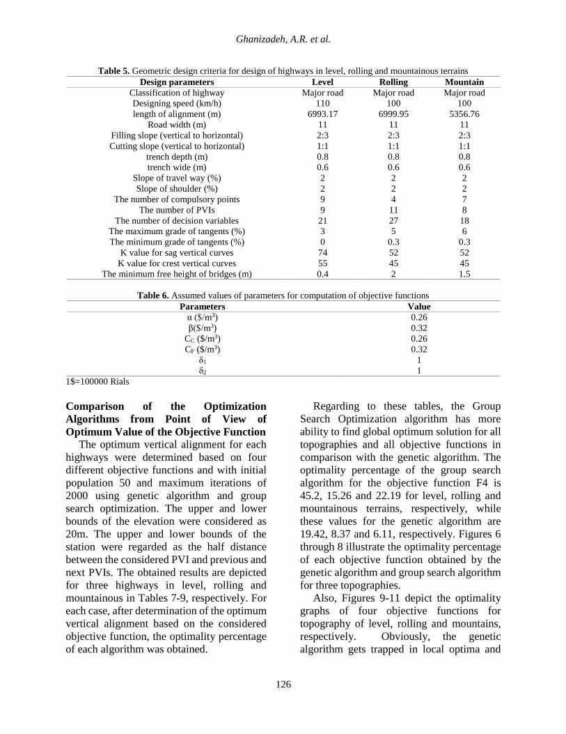
The geometric design criteria for each

terrains are given in Table 5. Horizontal

alignment of three paths in level, rolling and

mountainous terrains has been illustrated in

Figure 5. The considered parameters for

calculation of the objective function are listed

in Table 6.

Following the design of highways by

AutoCAD Land Desktop 2009 software, an

expert highway engineer designed a

preliminary vertical alignment based on the

design restrictions. Then, the vertical

alignment data including station, elevation

and vertical length curve of PVIs and cross

section data including offset and elevation of

existing ground points as well as station,

elevation and free height of bridges were

exported into text files. These files are input

files for the MATLAB 2014 optimization

program.

Setting the Parameters of the Optimization

Algorithms

For the genetic algorithm, the changing

range of the crossover and mutation

probabilities were regarded in [0.7-1] and

[0.1-0.4], respectively. The optimum vertical

alignment of a level highway with population

50 and generation 2000 and the first objective

function was considered to select the best

values of these two parameters. After a try

and error processes the best values for

crossover and mutation probabilities were

identified as 0.9 and 0.4, respectively. The

Group Search Optimization (GSO) algorithm

consists of three design parameters of max ,

maxI and max that for each one, a random

vector was set between 0 and 1 witch their

values variate in each repetition.

(a) Level Terrain

(b) Rolling Terrain

(c) Mountainous Terrain

Fig. 5. Existing paths in level, rolling and mountainous terrains


126

Table 5. Geometric design criteria for design of highways in level, rolling and mountainous terrains

Mountain Rolling Level Design parameters

Major road

100

5356.76

11

2:3

1:1

0.8

0.6

2

2

7

8

18

Major road

100

6999.95

11

2:3

1:1

0.8

0.6

2

2

4

11

27

Major road

110

6993.17

11

2:3

1:1

0.8

0.6

2

2

9

9

21

Classification of highway

Designing speed (km/h)

length of alignment (m)

Road width (m)

Filling slope (vertical to horizontal)

Cutting slope (vertical to horizontal)

trench depth (m)

trench wide (m)

Slope of travel way (%)

Slope of shoulder (%)

The number of compulsory points

The number of PVIs

The number of decision variables

6

0.3

52

45

1.5

5

0.3

52

45

2

3

0

74

55

0.4

The maximum grade of tangents (%)

The minimum grade of tangents (%)

K value for sag vertical curves

K value for crest vertical curves

The minimum free height of bridges (m)

Table 6. Assumed values of parameters for computation of objective functions Parameters Value

α )$/m3) 0.26

β)$/m3) 0.32

CC ($/m3) 0.26

CF ($/m3) 0.32

δ1 1

δ2 1

1$=100000 Rials

Comparison of the Optimization

Algorithms from Point of View of

Optimum Value of the Objective Function

The optimum vertical alignment for each

highways were determined based on four

different objective functions and with initial

population 50 and maximum iterations of

2000 using genetic algorithm and group

search optimization. The upper and lower

bounds of the elevation were considered as

20m. The upper and lower bounds of the

station were regarded as the half distance

between the considered PVI and previous and

next PVIs. The obtained results are depicted

for three highways in level, rolling and

mountainous in Tables 7-9, respectively. For

each case, after determination of the optimum

vertical alignment based on the considered

objective function, the optimality percentage

of each algorithm was obtained.

Regarding to these tables, the Group

Search Optimization algorithm has more

ability to find global optimum solution for all

topographies and all objective functions in

comparison with the genetic algorithm. The

optimality percentage of the group search

algorithm for the objective function F4 is

45.2, 15.26 and 22.19 for level, rolling and

mountainous terrains, respectively, while

these values for the genetic algorithm are

19.42, 8.37 and 6.11, respectively. Figures 6

through 8 illustrate the optimality percentage

of each objective function obtained by the

genetic algorithm and group search algorithm

for three topographies.

Also, Figures 9-11 depict the optimality

graphs of four objective functions for

topography of level, rolling and mountains,

respectively. Obviously, the genetic

algorithm gets trapped in local optima and


127

cannot converge to the global optimum

solution, whereas the group search algorithm

converges to the global optimum solution

with a suitable number of iterations.

Table 7. Initial and optimized objective function values for highway designed in the level terrain

GSO optimality

percentage GSO

GA optimality

percentage GA Manual Objective function

42.71 518.39 13.2 785.44 904.87 F1 function values (m) 43.74 162.9 13.26 251.2 289.6 F2 function values ($/m2) 44.11 68375.65 16.12 102624.74 122346.27 F3 function values (m3) 45.2 21433 19.42 31517.6 39113 F4 function values ($)

Table 8. Initial and optimized objective function values for highway designed in the rolling terrain

GSO optimality

percentage GSO

GA optimality


23.71 2195.43 16.17 2412.42 2877.81 F1 function values (m) 29.17 619.9 21.93 683.3 875.2 F2 function values ($/m2) 13.25 581757.52 4.99 637124.37 670590.99 F3 function values (m3) 15.26 166743 8.37 180289.6 196761.2 F4 function values ($)

Table 9. Initial and optimized objective function values for highway designed in the mountainous terrain

GSO optimality

percentage GSO

GA optimality


22.44 359.26 5.58 437.35 463.22 F1 function values (m) 23.95 11.27 5.66 13.98 14.82 F2 function values ($/m2) 20.85 72629.02 6.16 86104.8 91761.6 F3 function values (m3) 22.19 22824.6 6.11 27541.2 29333.2 F4 function values ($)

Fig. 6. Optimality percentage in level terrain

Fig. 7. Optimality percentage in rolling terrain

13.213.26 16.12

19.42

42.71 43.74 44.11 45.2

0

10

20

30

40

50

60

F1 F2 F3 F4

Op

tim

ali

ty p

erce

nta

ge GA GSO

16.17

21.93

4.99

8.37

23.71

29.17

13.2515.26

0

5

10

15

20

25

30

35

F1 F2 F3 F4

Op

tim

ali

ty p

erce

nta

ge GA GSO


128

Fig. 8. Optimality percentage in mountain terrain

(a) F1 function values

(b) F2 function values

(c) F3 function values

(d) F4 function values

Fig. 9. Performance of different algorithms to find optimum solution (level terrain)

5.58 5.66 6.16 6.11

22.4423.95

20.85 22.19

0

5

10

15

20

25

30

F1 F2 F3 F4O

pti

mali

typ

erce

nta

ge

GA GSO

400

600

800

1000

0 200 400 600 800 1000 1200 1400 1600 1800 2000

valu

e of

F1

fun

ctio

n (

m)

Iterations

GA GSO

150

180

210

240

270

300

0 200 400 600 800 1000 1200 1400 1600 1800 2000

valu

e of

F2

fun

ctio

n (

$/m

2)

Iterations

GA GAO

60000

110000

160000

0 500 1000 1500 2000

valu

e of

F3

fun

ctio

n (

m3)

Iterations

GA GSO

20000

30000

40000

0 200 400 600 800 1000 1200 1400 1600 1800 2000

valu

e of

F4

fun

ctio

n (

$)

Iterations

GA GSO


129





Fig. 10. Performance of different algorithms to find optimum solution (rolling terrain)


2100

2200

2300

2400

2500

2600

0 200 400 600 800 1000 1200 1400 1600 1800 2000

valu

e of

F1

fu

nct

ion

(m)

Iterations

GA GSO

600

625

650

675

700

725

750

0 200 400 600 800 1000 1200 1400 1600 1800 2000

valu

e of

F2

fu

nct

ion

($/m

2)

Iterations

GA GSO

575000

625000

675000

725000

0 200 400 600 800 1000 1200 1400 1600 1800 2000

valu

e of

F3

fu

nct

ion

(m3)

Iterations

GA GSO

160000

170000

180000

190000

200000

0 200 400 600 800 1000 1200 1400 1600 1800 2000

valu

e of

F4

fu

nct

ion

($)

Iterations

GA GSO

300

350

400

450

500

0 200 400 600 800 1000 1200 1400 1600 1800 2000

valu

e of

F1

fu

nct

ion

(m)

Iterations

GA GSO


130




Fig. 11. Performance of different algorithms to find optimum solution (mountainous terrain)

To evaluate the performance of Ga and

GSA algorithms, run time for each repetition

and repetitions to find optimum solution are

presented in Figures 12 and 15, in the

respective order.

According to Figures 12 and 13, the

required run time for the GSO is less than that

of the genetic algorithm in case of all terrains.

Furthermore, the run time of objective

function F3 and F4 is approximately equal

and several times more than that for objective

functions F1 and F2 in all terrains. Moreover,

it can be seen that the run time of objective

function F1 is approximately half of that for

objective function F2. In the maximum state

when using genetic algorithm, the run time of

F4 is 150 times more than that of F1 for the

rolling topography. This value for the group

search algorithm is about 265.

The first optimum solution for the level

topography using the GSO algorithm and for

F1, F2, F3 and F4 are respectively is find at

iterations 5, 5, 4 and 2, while those for the

genetic algorithm are at iterations 8, 11, 5,

and 4 for the four objective functions,

respectively. In the rolling topography, the

first obtained optimum solutions using GSO

and for F1, F2, F3 and F4 are respectively at

iteration of 1, 1, 6 and 4, while those for the

genetic algorithm are at iterations 1, 1, 13,

and 3 for the four objective functions,

respectively. In the mountainous terrain, the

11

12

13

14

15

16

0 200 400 600 800 1000 1200 1400 1600 1800 2000

valu

e of

F2

fu

nct

ion

($/m

2)

Iterations

GA GSO

65000

75000

85000

95000

0 200 400 600 800 1000 1200 1400 1600 1800 2000

valu

e of

F3

fu

nct

ion

(m3)

Iterations

GA GSO

22000

24000

26000

28000

30000

0 200 400 600 800 1000 1200 1400 1600 1800 2000

valu

e of

F4

fu

nct

ion

($)

Iterations

GA GSO


131

GSO algorithm found the first optimum

solutions at the first iteration for all four

objective functions, while the genetic

algorithm found those at iterations 1, 3, 1 and

1, respectively. Figures 14 and 15

demonstrate that the genetic algorithm after a

limit number of the iterations gets trapped in

the local optima and couldn’t find the global

optimum solution.

Comparison of the Objective Functions in

Terms of Earthwork Cost Reduction

The main objective of optimization of a

vertical alignment is finding a vertical

alignment that implies the minimum

earthwork cost of the project. Hence, other

objective functions (F1 to F3) would be

considered when they can reduce the

earthwork cost to the minimum level. In order

to evaluate this issue, the Earthwork cost (the

F4 objective function) is calculated for the

optimized vertical alignments based on the

other objective functions. Tables 10-12

depicted the earthwork cost values for three

terrains obtained by GA and GSO.

Fig. 12. Run time for each iteration in case of GA algorithms

Fig. 13. Run time for each iteration in case of GSO algorithms

Fig. 14. The latest optimum iteration in case of GA algorithms

0.28 0.286 0.2030.538 0.536 0.319

31.459

41.468

21.921

31.583

41.488

21.912

0

10

20

30

40

50

LEVEL ROLLING MOUNTAIN

Tim

e (s

ec)

F1 F2 F3 F4

0.093 0.089 0.0430.217 0.221 0.097

16.917

23.657

11.376

16.996

23.582

11.343

0

5

10

15

20

25

30


Tim

e (s

ec)

F1 F2 F3 F4

65

986

77

202

791

512

222

1963 1824

195

1051

140

500

1000

1500

2000


Th

e la

test

op

tim

um

ite

rati

on

F1 F2 F3 F4


132

Fig. 15. The latest optimum iteration in case of GSO algorithms

Table 10. Earthwork cost for optimized vertical alignments in level terrain

GSO GA Manual Objective function 22776.6 31624.2 39113 F1 ($)

23516.6 31621.6 39113 F2 ($) 21453.2 32668.2 39113 F3 ($) 21433 31517.6 39113 F4 ($)

Table 11. Earthwork cost for optimized vertical alignments in rolling terrain

GSO GA Manual Objective function 189139.6 194347 196761.2 F1 ($)

205724.2 212319.2 196761.2 F2 ($) 167397 181901.2 196761.2 F3 ($)

166743.2 180289.6 196761.2 F4 ($)

Table 12. Earthwork cost for optimized vertical alignments in mountain terrain

GSO GA Manual Objective function 22856.4 27886 29333.2 F1 ($)

22845.6 27581 29333.2 F2 ($) 22906.4 27562.4 29333.2 F3 ($) 22824.6 27541.2 29333.2 F4 ($)

As it is expected, the objective function F4

obtained less Earthwork cost values in

comparison with other three objective

functions. Figures 16 and 17 respectively

show the optimality of the earthwork cost for

the vertical alignment obtained from different

objective functions and by two optimization

algorithms.

The ground line, the preliminary vertical

alignment, as well as optimal vertical

alignment for GSO algorithm in three

different terrains of level, rolling and

mountainous are presented in Figures 18

through 20 in the respective order. As shown,

the objective functions F3 and F4 is very

close in terms of the optimality percentage. In

other words, regarding the minimization of

the earthwork cost (4th objective function),

pretty close results can be expected by

minimizing either the sum of cut and fill

volumes (3rd objective function) or the

Earthwork cost (4th objective function).

The optimality percentage of objective

functions F1 and F2 is greatly dependent to

the condition of the highway cross sections.

For instance, in this research, it can be

observed that in the highways designed in the

level and mountain terrains, objective

function F1 and F2 are able to find optimum

vertical alignment in terms of Earthwork cost,

while for the rolling topography, these

objective functions cannot find the vertical

alignment with the minimum Earthwork cost.

841

1846

231

1694

1950

712

1913 1934

568

788

1030

1432

0

500

1000

1500

2000

2500


Th

e la

test

op

tim

um

ite

rati

on F1 F2 F3 F4


133

Fig. 16. Optimality percentage of Earthwork cost using genetic algorithm

Fig. 17. Optimality percentage of Earthwork cost using group search optimization

Fig. 18. Longitudinal profile in case of highway designed in level terrain

Fig. 19. Longitudinal profile in case of highway designed in rolling terrain

18.99

1.23

4.93

19.15

-7.91

5.97

16.48

7.55 6.04

19.42

8.376.11

-10

-5

0

5

10

15

20

25

LEVEL ROLLING MOUNTAINOp

tim

alit

y p

erce

nta

ge

F1 F2 F3 F4

41.77

3.87

22.08

39.88

-4.56

22.12

45.15

14.92

21.91

45.2

15.2622.19

-20

-10

0

10

20

30

40

50

LEVEL ROLLING MOUNTAINOp

tim

alit

y p

erce

nta

ge

F1 F2 F3 F4

1980

1985

1990

1995

2000

2005

2010

2015

2020

2025

0 500 1000 1500 2000 2500 3000 3500 4000 4500 5000 5500 6000 6500 7000

Ele

vat

ion (

m)

Station (m)

Existing Ground Initial project line GSO Bridge

1900

1925

1950

1975

2000

2025

2050

2075

2100

0 500 1000 1500 2000 2500 3000 3500 4000 4500 5000 5500 6000 6500 7000

Ele

vat

ion (

m)

Station (m)



134

Fig. 20. Longitudinal profile in case of highway designed in mountainous terrain

As shown, for objective function F2, the

resulting optimum solution by this objective

function leads to increased Earthwork cost.

Consequently, it would be necessary to apply

earthwork volumes or Earthwork cost as the

objective function for optimizing the vertical

alignment. Indeed, the Earthwork cost cannot

be minimized by designing the vertical

alignment as close as possible to the existing

ground at the highway centerline.

Results of this study show that the manual

design of vertical alignment which considers

only the minimizing distance between

vertical alignment and ground line at

centerline is not able to reach the vertical

alignment with minimum earthwork cost. In

fact, human design does not have the ability

to consider all cross sections for designing an

optimal vertical alignment and so the use of

computer algorithms for optimizing the

project line is very necessary.

This research also confirms that the

applying a powerful optimization algorithm

such as GSO can improve finding optimum

vertical alignment in terms of both optimality

percentage as well as run time.

CONCLUSIONS

The aim of this paper was comparing several

objective functions for optimization of the

highways vertical alignment. These objective

functions were considered as the sum of the

absolute value of variance between the

vertical alignment and the existing ground

(F1), the sum of the absolute value of

variance between the vertical alignment and

the existing ground regarding different

weights for cuts and fills (F2), the sum of cut

and fill volumes (F3), and the Earthwork cost

(F4).

Constraints for this optimization problem

were considered as maximum and minimum

of tangents grade, minimum elevation of

compulsory points, non-overlapping of

vertical curves and minimum length of

vertical curves. To determine the earthwork

volumes precisely, a computer program was

implemented in the MATLAB 2014 and then

it was validated using AutoCAD Land

Desktop 2009. This comparison illustrated

that the developed code is able to calculate

the highway earthwork volumes with an error

about 5%.

Results of this study indicates that contrary

to the GA, the GSO algorithm is capable of

finding the global optimum solution in all

terrains and all objective functions more

efficiently. In fact, after a few repetitions, the

genetic algorithm gets trapped into the local

optima and cannot find the global optimal

solution, whereas the GSO algorithm

converges to the global optimal solution at an

appropriate speed. The run time of the GSO

is also less than that of the GA for all terrains.

From the perspective of run time, the run

time of objective function F3 and F4 is

approximately same and several times more

1950

2000

2050

2100

2150

2200

2250

0 500 1000 1500 2000 2500 3000 3500 4000 4500 5000 5500

Ele

vat

ion (

m)

Station (m)



135

than that for F1 and F2 for both optimization

algorithms. The run time of F1 is about half

run time of F2. In the most extreme case, the

run time of objective function F4 is about 265

times more than that the required run time for

objective F1.

Results of this study also show that the

vertical alignment resulted from minimizing

sum of cut and fill volumes (F3 objective

function) is very close to the vertical

alignment resulted from minimizing the

earthwork cost (F4 objective function).

In general, it can be said that the sum of

earthwork volumes or the sum of earthwork

costs are the most appropriate objective

functions for optimization of vertical

alignment. In other words, the earthwork cost

cannot be essentially minimized by designing

the vertical alignment as close as possible to

the existing ground at the highway centerline.

REFERENCES

AASHTO. (2011). (American Association of State

Highway and Transportation Officials). (2011).

Policy on geometric design of highways and

streets, Washington, D.C., 1(990), 158.

Abbey, L. (1992). Highways, Van Nostrand Reinhold,

New York.

Al-Sobky, S. )2014(. “An optimization approach for

highway vertical alignment using the earthwork

balance condition”, World Applied Sciences

Journal, 29(7), 884-891.

AUSTROADS Guide. (1993). Rural road design,

guide to the geometric design of rural roads,

AUSTROADS Publication, Australia.

Bababeik, M. and Monajjem, M. )2012(. “Optimizing

longitudinal alignment in railway with regard to

construction and operating costs”, Journal of

Transportation Engineering, 138(11), 1388-1395.

Banks, J. (2002). Introduction to Transportation

Engineering, McGraw-Hill, New York.

Beiranvand, V., Hare, W., Lucet, Y. and Hossain, S.

)2017(. “Multihaul quasi network flow model for

vertical alignment optimization”, Engineering

Optimization, 49(10), 1777-1795.

CALTRANS. (1995). Highway design manual,

California Department of Transportation

Publication, America.

Dabbour, E., Raahemifar, K. and Easa, S. (2002).

“Optimum vertical curves for highway profiles

using nonlinear Optimization”, Annual Conference

of the Canadian Society for Civil Engineering,

Montreal, Quebec.

Easa, S.M. )1988(. “Selection of roadway grades that

minimize earthwork cost using linear

programming”, Transportation Research Part A:

General, 22(2), 121-136.

Easa, S.M. )1999(, “Optimum vertical curves for

highway profiles”, Journal of Surveying

Engineering, 125(3), 147-157.

Fwa, T.F., Chan, W.T. and Sim, Y.P. )2002(. “Optimal

vertical alignment analysis for highway design”,

Journal of Transportation Engineering, 128(5),

395-402.

Garber, N.J. and Hoel, L.A. (2014). Traffic and

Highway Engineering, Timothy Anderson, United

States of America.

Ghanizadeh, A.R. and Heidarabadizadeh, N. (2018).

“Optimization of vertical alignment of highways in

terms of Earthwork cost using colliding bodies

Optimization algorithm”, International Journal of

Optimization in Civil Engineering, 8(4), 657-674.

Göktepe, A.B., Altun, S. and Ahmedzade, P. (2010).

“Optimization of vertical alignment of highways

utilizing discrete dynamic programming and

weighted ground line”, Journal of Engineering and

Environmental Sciences, 33(2), 105-116.

Göktepe, A.B., Lav, A.H., Altun, S. and Altıntaş, G.

)2008(. “Fuzzy decision support system to

determine swell/shrink factor affecting earthwork

optimization of highways”, Mathematical and

Computational Applications, 13(1), 61-70.

Göktepe, A.B., Lav, A.H. and Altun, S. (2009).

“Method for optimal vertical alignment of

highways”, Proceedings of the Institution of Civil

Engineers, ICE, 162(4), 177-188.

Hare, W., Hossain, S., Lucet, Y. and Rahman, F.

)2014(. “Models and strategies for efficiently

determining an optimal vertical alignment of

roads”, Computers and Operations Research,

44(2014), 161-173.

Hare, W., Lucet, Y. and Rahman, F. )2015(. “A mixed-

integer linear programming model to optimize the

vertical alignment considering blocks and side-

slopes in road construction”, European Journal of

Operational Research, 241(3), 631-641.

He, S., Wu, Q.H. and Saunders, J.R. )2009(. “Group

search optimizer: an optimization algorithm

inspired by animal searching behavior”, IEEE

Transactions on Evolutionary Computation, 13(5),

973-990.

He, S., Wu, Q.H. and Saunders, J.R. )2006(. “A group

search optimizer for neural network training”,

Proceedings of the 5th International Conference on

Computational Science and Its Applications,

Glasgow.


136

He, S., Wu, Q.H. and Saunders, J.R. )2006(. “A novel

group search optimizer inspired by animal

behavioural ecology”, IEEE International

Conference on Evolutionary Computation,

Vancouver.

Hadiwardoyo, S.P., Correia, A.G. and Pereira, P.

(2017). “Pavement maintenance optimization

strategies for national road network in Indonesia

applying Genetic Algorithm”, Procedia

Engineering, 210, 253-260.

Holland, J.H. (1975). Adaptation in natural and

artificial systems: An introductory analysis with

application to biology, control, and artificial

intelligence, Oxford, England: U Michigan Press.

Husseinzadeh Kashan, A., Jalili, S. and Karimiyan, S.

(2018). “Optimum structural design with discrete

variables using league championship algorithm”,

Civil Engineering Infrastructures Journal, 51(2),

253-275.

IMPO. (2012), Iran highway geometric design, Code

No. 415, Tehran, Iran.

Kazemi, S.F. and Shafahi, Y. )2013(. “An integrated

model of parallel processing and PSO algorithm for

solving optimum highway alignment problem”,

Proceedings of the 27th European Conference on

Modelling and Simulation, ECMS, Ålesund.

Li, W., Pu, H., Zhao, H. and Liu, W. (2013).

“Approach for optimizing 3D highway alignments

based on two-stage Dynamic Programming”,

Journal of Software, 8(11), 2967-2973.

Mahmoodabadi, M. and Nemati, A. )2016(. “A novel

adaptive genetic algorithm for global optimization

of mathematical test functions and real-world

problems”, Engineering Science and Technology,

an International Journal, 19(4), 2002-2021.

Mil, S. and Piantanakulchai, M. )2013(. “Vertical

Alignment optimization using Customized

Polynomial Regression model”, Proceedings of the

10th Conference of Eastern Asia Society for

Transportation Studies, Taipeh.

Moosavian, N. and Jaefarzade, M.R. (2015). “Particle

Swarm Optimization for hydraulic analysis of

water distribution systems”, Civil Engineering

Infrastructures Journal, 48(1), 9-22.

Papacostas, C.S. and Prevedouros, P.D. (1993).

Transportation engineering and planning, TRID,

Washington, DC.

Rahman, F. )2012(. “Optimizing the Vertical

Alignment under earthwork block removal

constraints in road construction”, M.Sc. Thesis,

University of British Columbia.

Shafahi, Y. and Bagherian, M. )2013(. “A customized

Particle Swarm method to solve highway

alignment optimization problem”, Computer-

Aided Civil and Infrastructure Engineering, 28 (1),

52-67.

Tunahoglu, N. and Soycan, M. )2014(. “A novel route

design metodology based on minimizing level

differences between grade and ground line,

Geodetski Vestnik”, Journal of the Association of

Surveyors of Slovenia, 58(1), 140-154.

Wang, W., Lukas, K. and Ji, Y. )2011(. “Two-stage

optimization of highway vertical alignment using

Genetic Algorithms”, Proceedings of the 1st

International Conference on Forum

Bauinformatik, University of Cork.

https://www.researchgate.net/conference-event/EASTS_Conference-of-Eastern-Asia-Society-for-Transportation-Studies_2013/1431

https://www.researchgate.net/conference-event/EASTS_Conference-of-Eastern-Asia-Society-for-Transportation-Studies_2013/1431

Effect of Objective Function on the Optimization of Highway Vertical ...€¦ · the vertical...

Documents

Transcript of Effect of Objective Function on the Optimization of Highway Vertical ...€¦ · the vertical...