Effect of N on F, p, 𝜂2, 𝜔2, Cohen’s f

b1 b2

a1 n n

a2 n n

a3 n n

Factor B

Factor A

3(A) x 2(B) Factorial Design

within-cell distributions

marginal distributions of A (ignoring B)

a1 a2 a3

3540

4550

5560

n=6

A Level

Y

b1 b2

3540

4550

5560

n=6

B Level

Y

a1.b1 a2.b1 a3.b1 a1.b2 a2.b2 a3.b2

3540

4550

5560

n=6

Cell

Y

marginal distributions of B (ignoring A)

n=6

n = 6

partial eta-squared (A) = 54.669 / (54.669+225.478) = 0.195partial omega-squared (A) = 0.128Cohen’s f (A) = 0.38

What happens as we increase N?

n = 8

partial eta-squared (A) = 64.97 / (64.97 +351.54) = 0.156partial omega-squared (A) = 0.11Cohen’s f (A) = 0.35

n = 16

partial eta-squared (A) = 66.53 / (66.53 +540.45) = 0.110partial omega-squared (A) = 0.09Cohen’s f (A) = 0.31

n = 32

partial eta-squared (A) = 223.57 / (223.57 +1214.26) = 0.155partial omega-squared (A) = 0.14Cohen’s f (A) = 0.41

n = 64

partial eta-squared (A) = 254.14 / (254.14 + 2872.45) = 0.081partial omega-squared (A) = 0.08Cohen’s f (A) = 0.29

within-cell distributions

marginal distributions of A (ignoring B)

marginal distributions of B (ignoring A)

a1 a2 a3

3540

4550

5560

n=64

A Level

Y

b1 b2

3540

4550

5560

n=64

B Level

Y

a1.b1 a2.b1 a3.b1 a1.b2 a2.b2 a3.b2

3540

4550

5560

n=64

Cell

Y

n=64

a1.b1 a2.b1 a3.b1 a1.b2 a2.b2 a3.b2

3540

4550

5560

n=8

Cell

Y

a1.b1 a2.b1 a3.b1 a1.b2 a2.b2 a3.b2

3540

4550

5560

n=16

Cell

Y

a1.b1 a2.b1 a3.b1 a1.b2 a2.b2 a3.b2

3540

4550

5560

n=32

Cell

Y

a1.b1 a2.b1 a3.b1 a1.b2 a2.b2 a3.b2

3540

4550

5560

n=64

Cell

Y

within-cell distributions

marginal distributions of A (ignoring B)

a1 a2 a3

3540

4550

5560

n=8

A Level

Y

a1 a2 a3

3540

4550

5560

n=16

A Level

Y

a1 a2 a3

3540

4550

5560

n=32

A Level

Y

a1 a2 a3

3540

4550

5560

n=64

A Level

Y

0 10 20 30 40 50 60 70

05

1015

20

Cell n

F va

lue

nearly 5-fold change in F

0 10 20 30 40 50 60 70

Cell n

1e-07

1e-06

1e-05

1e-041e-04

1e-03

1e-02

1e-01

p va

lue

p changes by more than a factor of 100,000

Cell n

p va

lue

Large changes in N produce large changes in F and p values.

0 10 20 30 40 50 60 70

0.0

0.1

0.2

0.3

0.4

0.5

0.6

Cell n

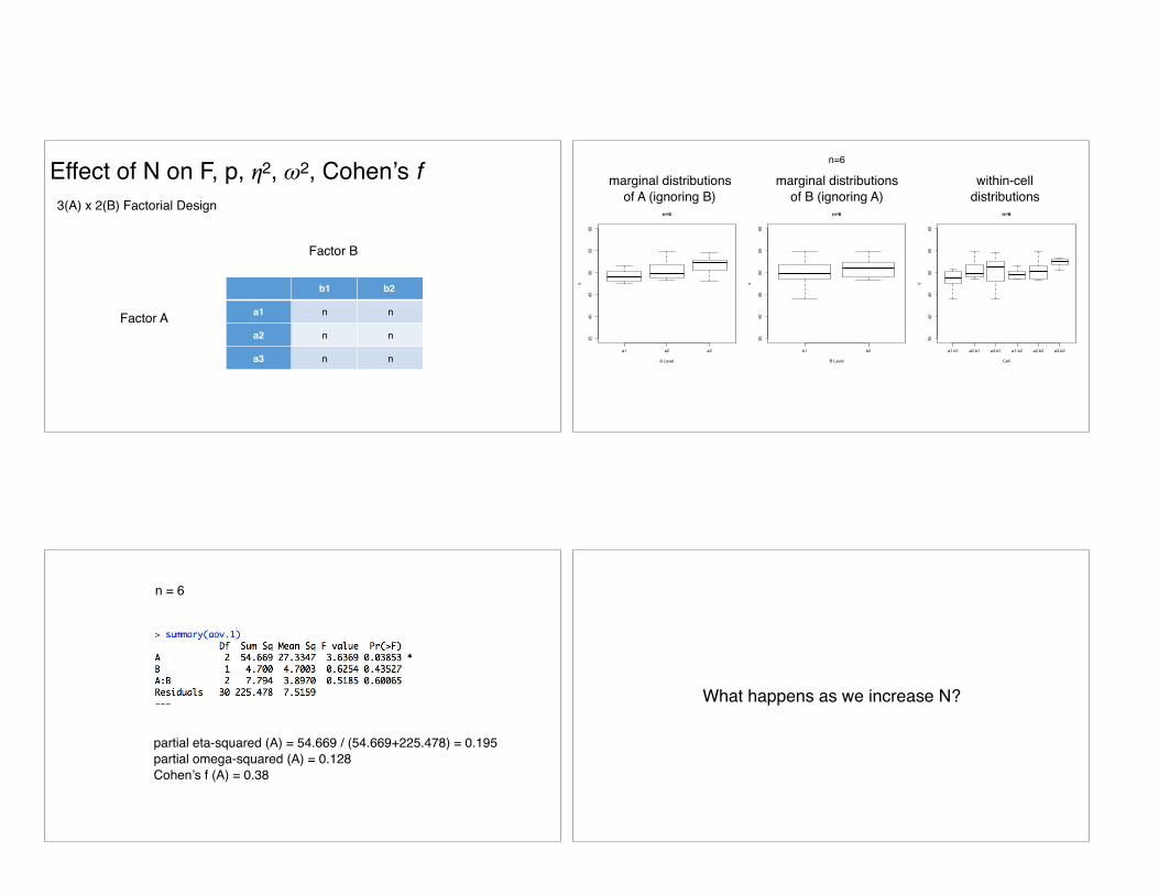
partial η2

partial ω2Cohens fMeasures of association

strength and effect size are not affected very much by large changes in N

Unbalanced Designsunequal n per cell

Bennett, PJ PSY710 Chapter 7

Table 2: Data from drinking study.

no alcohol alcohol Row Means

Michigan

13 15 1416 12Y11 =14

18 20 22 1921 23 17 1822 20Y12 = 20

Y1. = 18

Arizona13 15 18 1410 12 16 1715 10 14Y21 = 14

24 25 1716 18Y22 =20

Y2. = 15.9

Column Means Y.1 = 14 Y.2 = 20

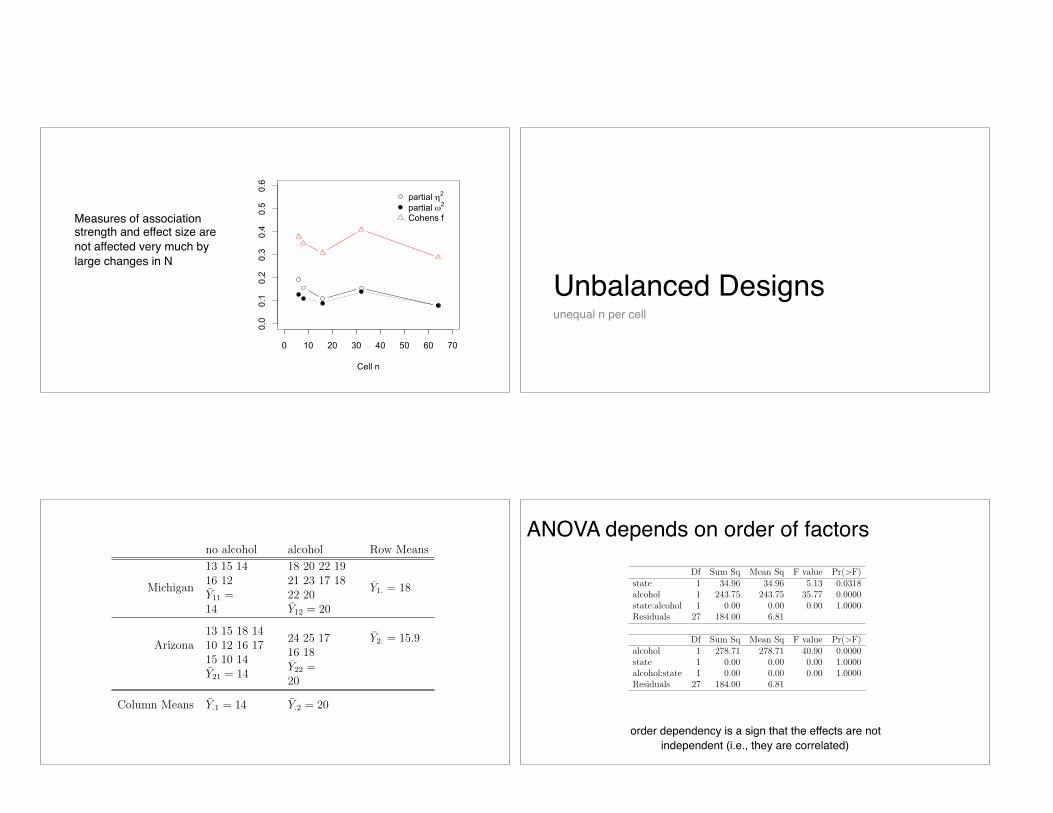
The fact that the row, column and interaction e↵ects are no longer orthogonal greatly complicatesthe analysis of variance. To see why, consider the following two linear models:

score ⇠ 1 + alcohol + state + alcohol : state (45)

score ⇠ 1 + state + alcohol + state : alcohol (46)

The ANOVA tables produced by R for Models 45 and 46 are presented in Table 3. Although themodels di↵er only in the order of terms, the sums of squares assigned by the models to the maine↵ects di↵er significantly.

Df Sum Sq Mean Sq F value Pr(>F)state 1 34.96 34.96 5.13 0.0318alcohol 1 243.75 243.75 35.77 0.0000state:alcohol 1 0.00 0.00 0.00 1.0000Residuals 27 184.00 6.81

Df Sum Sq Mean Sq F value Pr(>F)alcohol 1 278.71 278.71 40.90 0.0000state 1 0.00 0.00 0.00 1.0000alcohol:state 1 0.00 0.00 0.00 1.0000Residuals 27 184.00 6.81

Table 3: ANOVA tables for Model 1 (top) and Model 2 (bottom).

7.12.2 Proportional Cell Frequencies

Before I continue to discuss the problems associated with analyzing unbalanced data, I want todescribe a case where unbalanced data are not hard to analyze. Suppose we had 36 subjects fromMichigan, with 24 in the alcohol condition and 12 in the no-alcohol condition. Also, let’s supposethat there were 24 subjects from Arizona, with 16 in the alcohol condition and 8 in the no-alcoholcondition. In this case, the ratio of subjects in the alcohol and no-alcohol conditions is 2:1 at both

26

ANOVA depends on order of factors

Bennett, PJ PSY710 Chapter 7

Table 2: Data from drinking study.

no alcohol alcohol Row Means

Michigan

13 15 1416 12Y11 =14

18 20 22 1921 23 17 1822 20Y12 = 20

Y1. = 18

Arizona13 15 18 1410 12 16 1715 10 14Y21 = 14

24 25 1716 18Y22 =20

Y2. = 15.9

Column Means Y.1 = 14 Y.2 = 20

The fact that the row, column and interaction e↵ects are no longer orthogonal greatly complicatesthe analysis of variance. To see why, consider the following two linear models:

score ⇠ 1 + alcohol + state + alcohol : state (45)

score ⇠ 1 + state + alcohol + state : alcohol (46)

The ANOVA tables produced by R for Models 45 and 46 are presented in Table 3. Although themodels di↵er only in the order of terms, the sums of squares assigned by the models to the maine↵ects di↵er significantly.

Df Sum Sq Mean Sq F value Pr(>F)state 1 34.96 34.96 5.13 0.0318alcohol 1 243.75 243.75 35.77 0.0000state:alcohol 1 0.00 0.00 0.00 1.0000Residuals 27 184.00 6.81

Df Sum Sq Mean Sq F value Pr(>F)alcohol 1 278.71 278.71 40.90 0.0000state 1 0.00 0.00 0.00 1.0000alcohol:state 1 0.00 0.00 0.00 1.0000Residuals 27 184.00 6.81

Table 3: ANOVA tables for Model 1 (top) and Model 2 (bottom).

7.12.2 Proportional Cell Frequencies

Before I continue to discuss the problems associated with analyzing unbalanced data, I want todescribe a case where unbalanced data are not hard to analyze. Suppose we had 36 subjects fromMichigan, with 24 in the alcohol condition and 12 in the no-alcohol condition. Also, let’s supposethat there were 24 subjects from Arizona, with 16 in the alcohol condition and 8 in the no-alcoholcondition. In this case, the ratio of subjects in the alcohol and no-alcohol conditions is 2:1 at both

26

order dependency is a sign that the effects are not independent (i.e., they are correlated)

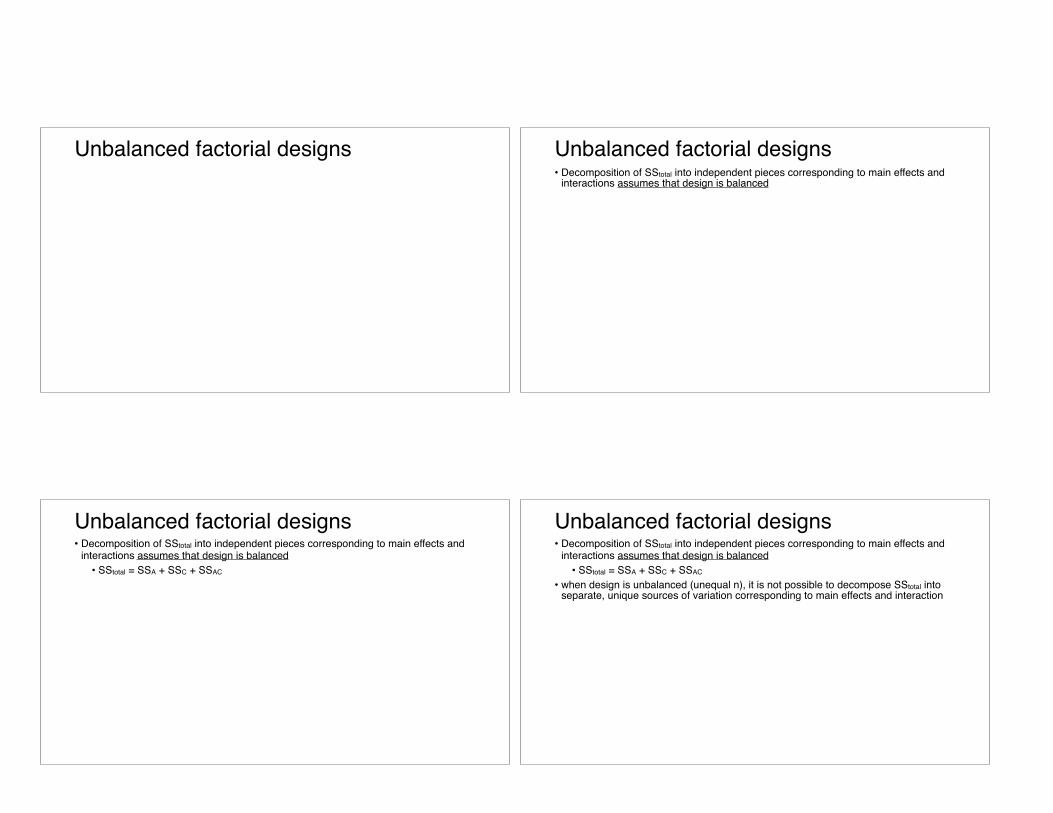
Unbalanced factorial designs Unbalanced factorial designs• Decomposition of SStotal into independent pieces corresponding to main effects and

interactions assumes that design is balanced

Unbalanced factorial designs• Decomposition of SStotal into independent pieces corresponding to main effects and

interactions assumes that design is balanced• SStotal = SSA + SSC + SSAC

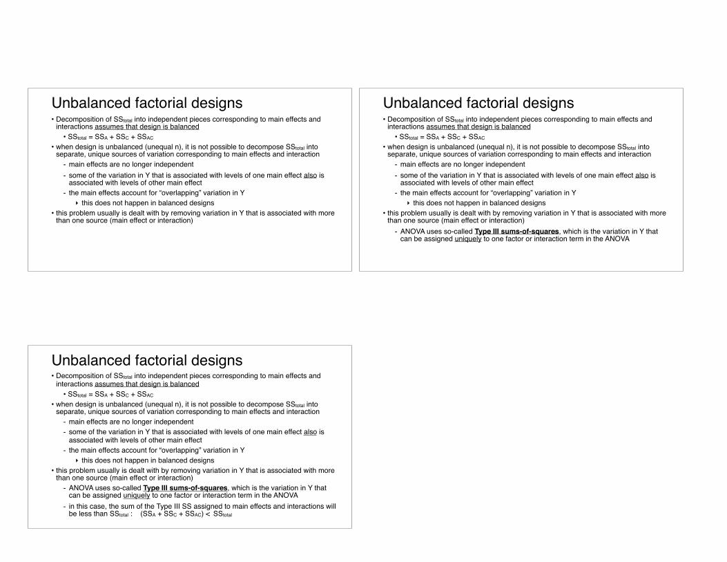
Unbalanced factorial designs• Decomposition of SStotal into independent pieces corresponding to main effects and

interactions assumes that design is balanced• SStotal = SSA + SSC + SSAC

• when design is unbalanced (unequal n), it is not possible to decompose SStotal into separate, unique sources of variation corresponding to main effects and interaction

Unbalanced factorial designs• Decomposition of SStotal into independent pieces corresponding to main effects and

interactions assumes that design is balanced• SStotal = SSA + SSC + SSAC

• when design is unbalanced (unequal n), it is not possible to decompose SStotal into separate, unique sources of variation corresponding to main effects and interaction- main effects are no longer independent

Unbalanced factorial designs• Decomposition of SStotal into independent pieces corresponding to main effects and

interactions assumes that design is balanced• SStotal = SSA + SSC + SSAC

• when design is unbalanced (unequal n), it is not possible to decompose SStotal into separate, unique sources of variation corresponding to main effects and interaction- main effects are no longer independent- some of the variation in Y that is associated with levels of one main effect also is

associated with levels of other main effect

Unbalanced factorial designs• Decomposition of SStotal into independent pieces corresponding to main effects and

interactions assumes that design is balanced• SStotal = SSA + SSC + SSAC

• when design is unbalanced (unequal n), it is not possible to decompose SStotal into separate, unique sources of variation corresponding to main effects and interaction- main effects are no longer independent- some of the variation in Y that is associated with levels of one main effect also is

associated with levels of other main effect- the main effects account for “overlapping” variation in Y

Unbalanced factorial designs• Decomposition of SStotal into independent pieces corresponding to main effects and

interactions assumes that design is balanced• SStotal = SSA + SSC + SSAC

• when design is unbalanced (unequal n), it is not possible to decompose SStotal into separate, unique sources of variation corresponding to main effects and interaction- main effects are no longer independent- some of the variation in Y that is associated with levels of one main effect also is

associated with levels of other main effect- the main effects account for “overlapping” variation in Y

‣ this does not happen in balanced designs

Unbalanced factorial designs• Decomposition of SStotal into independent pieces corresponding to main effects and

interactions assumes that design is balanced• SStotal = SSA + SSC + SSAC

• when design is unbalanced (unequal n), it is not possible to decompose SStotal into separate, unique sources of variation corresponding to main effects and interaction- main effects are no longer independent- some of the variation in Y that is associated with levels of one main effect also is

associated with levels of other main effect- the main effects account for “overlapping” variation in Y

‣ this does not happen in balanced designs• this problem usually is dealt with by removing variation in Y that is associated with more

than one source (main effect or interaction)

Unbalanced factorial designs• Decomposition of SStotal into independent pieces corresponding to main effects and

interactions assumes that design is balanced• SStotal = SSA + SSC + SSAC

• when design is unbalanced (unequal n), it is not possible to decompose SStotal into separate, unique sources of variation corresponding to main effects and interaction- main effects are no longer independent- some of the variation in Y that is associated with levels of one main effect also is

associated with levels of other main effect- the main effects account for “overlapping” variation in Y

‣ this does not happen in balanced designs• this problem usually is dealt with by removing variation in Y that is associated with more

than one source (main effect or interaction)- ANOVA uses so-called Type III sums-of-squares, which is the variation in Y that

can be assigned uniquely to one factor or interaction term in the ANOVA

Unbalanced factorial designs• Decomposition of SStotal into independent pieces corresponding to main effects and

interactions assumes that design is balanced• SStotal = SSA + SSC + SSAC

• when design is unbalanced (unequal n), it is not possible to decompose SStotal into separate, unique sources of variation corresponding to main effects and interaction- main effects are no longer independent- some of the variation in Y that is associated with levels of one main effect also is

associated with levels of other main effect- the main effects account for “overlapping” variation in Y

‣ this does not happen in balanced designs• this problem usually is dealt with by removing variation in Y that is associated with more

than one source (main effect or interaction)- ANOVA uses so-called Type III sums-of-squares, which is the variation in Y that

can be assigned uniquely to one factor or interaction term in the ANOVA- in this case, the sum of the Type III SS assigned to main effects and interactions will

be less than SStotal : (SSA + SSC + SSAC) < SStotal