1

Effect of Message Transmission PathDiversity on Status Age

Clement Kam, Member, IEEE, Sastry Kompella, Senior Member, IEEE, Gam D. Nguyen,and Anthony Ephremides, Life Fellow, IEEE

Abstract—This work focuses on status age, which is a metricfor measuring the freshness of a continually updated pieceof information (i.e., status) as observed at a remote monitor.Specifically, we study a system in which a sensor sends randomstatus updates over a dynamic network to a monitor. For thissystem, we consider the impact of having messages take differentroutes through the network on the status age. First, we considera network with plentiful resources (i.e., many nodes that canprovide numerous alternate paths), so that packets need not waitin queues at each node in a multihop path. This system is modeledas a single queue with an infinite number of servers, specificallyas an M/M/∞ queue. Packets routed over a dynamic networkmay arrive at the monitor out of order, which we account for inour analysis for the M/M/∞ model. We then consider a networkwith somewhat limited resources, so that packets can arrive outof order but also must wait in a queue. This is modeled as a singlequeue with two servers, specifically an M/M/2 queue. We presentthe exact approach to computing the analytical status age, andwe provide an approximation that is shown to be close to thesimulated age. We also compare both models with the M/M/1,which corresponds to severely limited network resources, andwe demonstrate the tradeoff between status age and unnecessarynetwork resource consumption.

Index Terms—Status age, dynamic networks, monitoring.

I. INTRODUCTION

WE consider a system in which a single source trackssome time-varying content. At various points in time,

it generates snapshots of the content and transmits it, withsome delay, to a receiver through a network. Our objectiveis to analyze the freshness of the content as viewed at thereceiver. A measure for this freshness, called the status age,has been defined in [1]. The primary question that we addressis the determination of the optimal frequency of status updatessuch that the average status age is minimized.

The status age captures the idea of freshness more preciselythan traditional metrics. For example, the delay for somepacket may be short, but if its transmission occurred a longtime ago, the information, as observed at the current time,is no longer fresh. As another example, throughput may behigh, such that packets arrive very frequently at the receiver.However, if the packets that arrive were generated a long timeago but delayed in a queue (at the source node or a relay node),

This paper was presented in part at the 2013 and 2014 IEEE InternationalSymposium on Information Theory.

C. Kam, S. Kompella and G. D. Nguyen are with the Naval Research Lab-oratory, Washington, DC 20375 USA (e-mail: clement.kam@nrl.navy.mil).

A. Ephremides is with the Electrical and Computer Engineering Departmentand Institute for Systems Research, University of Maryland, College Park, MD20742 USA.

Fig. 1. Real-time status updating system (green) with competing traffic(blue/red) over a network.

even recently received packets are no longer fresh. A differentmetric is needed to convey the freshness of information at thereceiver.

The concept of status age was first studied by Kaul et al.in the context of vehicular networks [2], [3]. They continuedthis work by characterizing the status age for a system con-sisting of a single-server queue with a first-come-first-serveddiscipline [1]. It was shown that when packets are generatedinfrequently, the monitor receives packets infrequently, andaverage status age can be large, i.e., what the monitor observes,on average, is an old status. Increasing the rate of packetgeneration (or sampling) initially reduces the age. However,at some point, packets are generated too frequently, whichbacklogs the queue; consequently, packets spend a long timein the queue before reaching the monitor. As a result, there isan optimal rate at which packets can be generated to minimizethe average age. In [4], a single server with last-come-first-served queue discipline was studied, and it was shown thatincreasing the utilization will always reduce the average agesince the newest packets are sent first and older packets haveno effect on the age. Additional work on status age focusedon systems with multiple sources [5] and the effect of packetmanagement [6].

In this paper, we consider a system in which a sourcegenerates packets containing snapshots of some content, butwe focus on transmitting these packets over a network to aremote monitor (Figure 1). We assume the source generatesthe packets with random (exponentially distributed) interarrivaltimes. This assumption facilitates analysis without impactingthe essential tradeoffs in the problem. Our goal is to char-acterize the average status age, where in this case, insteadof a simple single-server queue, we transmit over a dynamicnetwork, in which routes can change and packets can arriveout of order.

Due to the difficulty of modeling the routing delay through

2

a complex, dynamic network, we choose a simplified queue-based model to approximate such delay. For example, thesingle-server queue studied in [1] (an M/M/1 queue) canbe adopted as a simple model of network delay, but itsstrict in-order packet delivery is not reflective of realisticnetworks. Another way to model this system is to have packetsgenerated at the source immediately enter the network andreach the monitor after a random exponential time. This modelcan be viewed as a system with infinite memoryless servers(M/M/∞). Since the packets spend a random amount of timein the network, there is a possibility of packets arriving atthe monitor out of order, so that some packets that containinformation that is older than that which has already beenreceived. In the first part of this work, we analyze the M/M/∞model and show that increasing the rate of packet generationwill always result in a smaller average status age. However, itcomes at the cost of more useless, older packets in the system,which corresponds to a waste of network resources.

One shortcoming of modeling the network as an infinitenumber of memoryless servers is that it does not reflect thebehavior that packets that have been in the system for a longerduration are more likely to reach the monitor first, as in asingle server queue (which has strict in-order reception). Onthe other hand, a single server system does not reflect thedynamics of a network (e.g., changing topology) which allowfor packets to be received out of order. We are thus interestedin studying the intermediate case of a queue with c servers,1 < c <∞, which balances the out-of-order reception with thein-order queueing. The combination of queueing and out-of-order reception models the effect of transmission diversity overmultiple paths. In the second part of this work, we analyze thestatus age for a system with two servers (M/M/2) and providean approximation that is very close to the simulated age. Wealso provide numerical results to compare the performanceof the M/M/1, M/M/2, and M/M/∞ cases, demonstrating thetradeoff between the status age and the waste of networkresources as the number of servers varies.

II. STATUS AGE FOR THE M/M/∞ MODEL

A. System Model

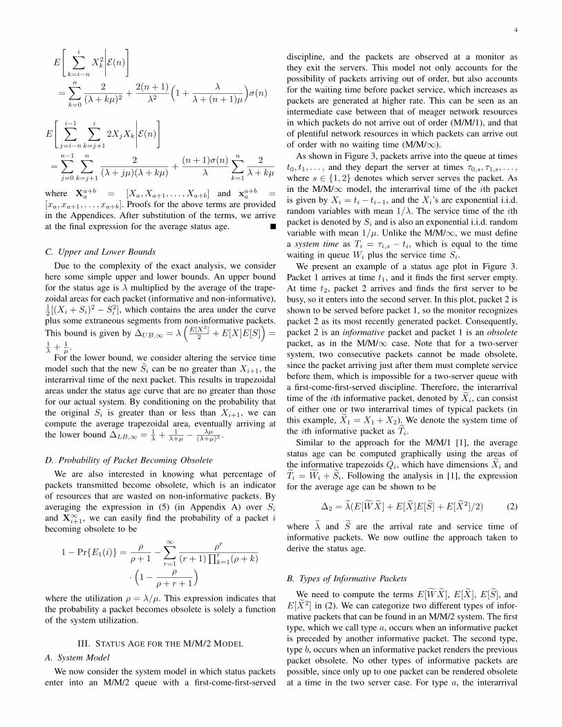
In this section, we study a system in which a sourcetransmits packets through a network to a remote monitor, andmodels it as an M/M/∞ queue. At transmission time, thesource transmits a packet containing the current informationand (since there are an infinite number of servers) it imme-diately begins service, so there is no aging occurring fromwaiting in a packet queue. A plot of the status age is shownin Figure 2, where transmissions occur at times t0, t1, . . ., andreceptions at the monitor occur at times τ0, τ1, . . ..

We refer to the time between packet generations as theinterarrival time Xi, i = 1, 2, . . ., which is equal to ti − ti−1.For the present case of an M/M/∞ queue, the transmissiontimes are identical to the packet generation times at thesource node. The interarrival times are modeled as random;consequently, the source does not have control over the exacttimes at which it can transmit updates. In our model, the Xi’sare i.i.d. exponential random variables with rate λ.

Fig. 2. Plot of status age for M/M/∞ system.

We call the time packet i spends in the network the servicetime Si, i = 1, 2, . . ., which is equal to τi − ti. For eachtransmission time Xi, the service time Si that immediatelyfollows is modeled as exponential with rate µ, and all the Si’sare i.i.d. and independent of the Xi’s. We consider this to be asimplified model of the random delay due to routing throughthe network, which is a result of various phenomena such aschanging link states, competing data traffic, and other networkdynamics.

We assume that packets enter the network instantaneouslyat each packet generation time. Due to the randomness ofthe service times, packets are not necessarily received at thedestination in the order in which they are transmitted, as notedin the introduction. A newly arriving packet provides usefulinformation only if it was generated later than all packets thathave previously arrived. Since the receiver does not update thestatus for such useless packets, the calculation of the status agebecomes complicated.

Definitions. We define the status age at time t ∆(t) asin [1]: ∆(t) = t−u(t), where u(t) is the timestamp of the mostrecent information at the receiver as of time t. In the M/M/∞system, the timestamp coincides with the transmission time ofthe packet. Given this definition, we can see that the status ageincreases linearly with t but is reset to a smaller value witheach packet received that contains newer information, resultingin the sawtooth pattern shown in Figure 2.

We define an informative packet as a packet received at thedestination that provides newer information than that whichhas been received up to that time. For example, in Figure 2,we say that packet 2 is an informative packet because it isreceived before packets 3, 4, and all future packets (τ2 <min(τ3, τ4, . . .)). However, packet 3 is not informative sinceit is received after packet 4 (τ3 > τ4). In terms of Xi’s andSi’s, the condition for a packet i being an informative packetis

Si < Sr +

r∑a=i+1

Xa ∀r = i+ 1, i+ 2, . . . .

We say that a packet p is rendered obsolete if some packetj transmitted after i (i.e., tj > ti) is received at the destination

3

before it (i.e., τj < τi), e.g., packet 4 renders packet 3 obsolete.An informative packet is one that is not rendered obsolete.

B. M/M/∞ Status Age

Using a graphical argument similar to that in [1], we canderive the status age for the M/M/∞ system, given in thefollowing theorem.

Theorem 1: The average status age for an M/M/∞ systemis given by

∆∞ = λ

∞∑n=0

Pr{E(n)}

[n∑j=0

(1

λ+ jµ

·( 2λ+ (n+ 2)µ

(λ+ (n+ 1)µ)(λ+ (n+ 2)µ)+

n∑k=j

1

λ+ kµ

))

+(n+ 1)σ(n)

λ

(2λ+ (n+ 2)µ

(λ+ (n+ 1)µ)(λ+ (n+ 2)µ)

+

n+1∑l=0

1

λ+ lµ

)](1)

where

σ(n) =

∞∑r=1

[λr

(n+ r + 1)∏rk=1(λ+ (n+ k)µ)

·(

1− λ

λ+ (n+ r + 1)µ

)]

and Pr{E(n)} = λnµ∏n+1k=1 (λ+kµ)

, where E(n) is the event thata packet is informative and that it renders n other packetsobsolete. The proof for Pr{E(n)} is given in Appendix A.

Proof: Similar to the approach in [1], we express theage by computing the total area of the trapezoids Q1, Q2, . . .in Figure 2 divided by the time elapsed T . In our case,the difference is that we have one trapezoid per informativepacket, rather than one for every packet transmitted, as in [1].Here, the bottom edges of the trapezoids can consist ofmultiple interarrival times due to some packets being renderedobsolete, rather than one interarrival time per trapezoid. Thesebottom edges are given as

∑pXp in our derivation, where

the Xp are the interarrival times of the informative packet andthe packets it renders obsolete. We ignore the pieces of thetrapezoidal areas that lie outside the edges of the time window,since they disappear in the limit as the window length Tapproaches infinity. The average age over T can be expressed

as

∆T =1

T∑

d∈D(T )

1

2

Sd +

d∑p=d−nd

Xp

2

− S2d

=1

T∑

d∈D(T )

1

2

d∑p=d−nd

Xp

2

+ 2Sd

d∑p=d−nd

Xp

=|D(T )|T

1

|D(T )|∑

d∈D(T )

1

2

[d∑

p=d−nd

X2p

+

d−1∑p=d−nd

d∑q=p+1

2XpXq + 2Sd

d∑p=d−nd

Xp

]

where D(T ) is the set of packet indices corresponding toinformative packets, and nd is the number of packets priorto packet d that are rendered obsolete, where d ∈ D(T ).

Let E1(i) be the event that a packet is informative andE2(n) be the event that a packet renders n packets obsolete,so we have E(n) = E1(i) ∩E2(n). Note that the steady-stateprobability of the event E(n) does not depend on i. Then,if we let T go to infinity, noting that limT→∞ |D(T )|/T =λPr{E1}, then the average age is given by

∆∞ = λPr{E1(i)}1

2

∞∑n=0

Pr{E2(n)|E1(i)}

·

(E

[i∑

k=i−n

X2k

∣∣∣∣∣E(n)

]E

[i−1∑

j=i−n

i∑k=j+1

2XjXk

∣∣∣∣∣E(n)

]

+ 2E[Si|E(n)]E

[i∑

k=i−n

Xk

∣∣∣∣∣E(n)

])

= λ1

2

∞∑n=0

Pr{E(n)}

(E

[i∑

k=i−n

X2k

∣∣∣∣∣E(n)

]

+ E

[i−1∑

j=i−n

i∑k=j+1

2XjXk

∣∣∣∣∣E(n)

]

+ 2E[Si|E(n)]E

[i∑

k=i−n

Xk

∣∣∣∣∣E(n)

]),

where i is the index of some informative packet when thesystem is in steady state. The conditional expectations in the∆∞ expression above are given by

E[Si|E(n)] =1

λ+ (n+ 1)µ

(1 +

λ

λ+ (n+ 2)µ

)

E

[i∑

k=i−n

Xk

∣∣∣∣∣E(n)

]

=

∫ i∑k=i−n

XkfX|E(n){Xmi−n = xii−n|E(n)}dxii−n

=

n∑k=0

1

λ+ kµ+n+ 1

λσ(n)

4

E

[i∑

k=i−n

X2k

∣∣∣∣∣E(n)

]

=

n∑k=0

2

(λ+ kµ)2+

2(n+ 1)

λ2

(1 +

λ

λ+ (n+ 1)µ

)σ(n)

E

[i−1∑

j=i−n

i∑k=j+1

2XjXk

∣∣∣∣∣E(n)

]

=

n−1∑j=0

n∑k=j+1

2

(λ+ jµ)(λ+ kµ)+

(n+ 1)σ(n)

λ

n∑k=1

2

λ+ kµ

where Xa+ba = [Xa, Xa+1, . . . , Xa+b] and xa+ba =

[xa, xa+1, . . . , xa+b]. Proofs for the above terms are providedin the Appendices. After substitution of the terms, we arriveat the final expression for the average status age.

C. Upper and Lower Bounds

Due to the complexity of the exact analysis, we considerhere some simple upper and lower bounds. An upper boundfor the status age is λ multiplied by the average of the trape-zoidal areas for each packet (informative and non-informative),12 [(Xi + Si)

2 − S2i ], which contains the area under the curve

plus some extraneous segments from non-informative packets.This bound is given by ∆UB,∞ = λ

(E[X2]

2 + E[X]E[S])

=1λ + 1

µ .For the lower bound, we consider altering the service time

model such that the new Si can be no greater than Xi+1, theinterarrival time of the next packet. This results in trapezoidalareas under the status age curve that are no greater than thosefor our actual system. By conditioning on the probability thatthe original Si is greater than or less than Xi+1, we cancompute the average trapezoidal area, eventually arriving atthe lower bound ∆LB,∞ = 1

λ + 1λ+µ −

λµ(λ+µ)3 .

D. Probability of Packet Becoming Obsolete

We are also interested in knowing what percentage ofpackets transmitted become obsolete, which is an indicatorof resources that are wasted on non-informative packets. Byaveraging the expression in (5) (in Appendix A) over Siand X∞i+1, we can easily find the probability of a packet ibecoming obsolete to be

1− Pr{E1(i)} =ρ

ρ+ 1−∞∑r=1

ρr

(r + 1)∏rk=1(ρ+ k)

·(

1− ρ

ρ+ r + 1

)where the utilization ρ = λ/µ. This expression indicates thatthe probability a packet becomes obsolete is solely a functionof the system utilization.

III. STATUS AGE FOR THE M/M/2 MODEL

A. System Model

We now consider the system model in which status packetsenter into an M/M/2 queue with a first-come-first-served

discipline, and the packets are observed at a monitor asthey exit the servers. This model not only accounts for thepossibility of packets arriving out of order, but also accountsfor the waiting time before packet service, which increases aspackets are generated at higher rate. This can be seen as anintermediate case between that of meager network resourcesin which packets do not arrive out of order (M/M/1), and thatof plentiful network resources in which packets can arrive outof order with no waiting time (M/M/∞).

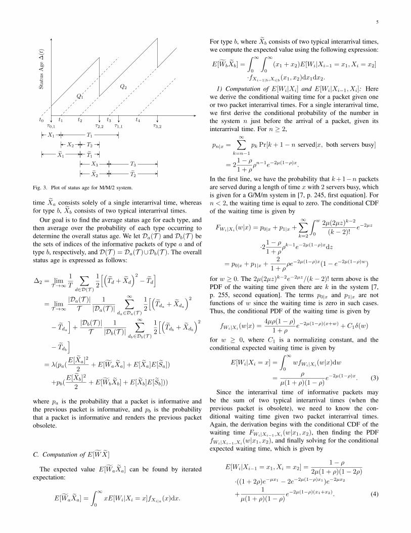
As shown in Figure 3, packets arrive into the queue at timest0, t1, . . . , and they depart the server at times τ0,s, τ1,s, . . . ,where s ∈ {1, 2} denotes which server serves the packet. Asin the M/M/∞ model, the interarrival time of the ith packetis given by Xi = ti− ti−1, and the Xi’s are exponential i.i.d.random variables with mean 1/λ. The service time of the ithpacket is denoted by Si and is also an exponential i.i.d. randomvariable with mean 1/µ. Unlike the M/M/∞, we must definea system time as Ti = τi,s − ti, which is equal to the timewaiting in queue Wi plus the service time Si.

We present an example of a status age plot in Figure 3.Packet 1 arrives at time t1, and it finds the first server empty.At time t2, packet 2 arrives and finds the first server to bebusy, so it enters into the second server. In this plot, packet 2 isshown to be served before packet 1, so the monitor recognizespacket 2 as its most recently generated packet. Consequently,packet 2 is an informative packet and packet 1 is an obsoletepacket, as in the M/M/∞ case. Note that for a two-serversystem, two consecutive packets cannot be made obsolete,since the packet arriving just after them must complete servicebefore them, which is impossible for a two-server queue witha first-come-first-served discipline. Therefore, the interarrivaltime of the ith informative packet, denoted by Xi, can consistof either one or two interarrival times of typical packets (inthis example, X1 = X1 +X2). We denote the system time ofthe ith informative packet as Ti.

Similar to the approach for the M/M/1 [1], the averagestatus age can be computed graphically using the areas ofthe informative trapezoids Qi, which have dimensions Xi andTi = Wi + Si. Following the analysis in [1], the expressionfor the average age can be shown to be

∆2 = λ(E[W X] + E[X]E[S] + E[X2]/2) (2)

where λ and S are the arrival rate and service time ofinformative packets. We now outline the approach taken toderive the status age.

B. Types of Informative Packets

We need to compute the terms E[W X], E[X], E[S], andE[X2] in (2). We can categorize two different types of infor-mative packets that can be found in an M/M/2 system. The firsttype, which we call type a, occurs when an informative packetis preceded by another informative packet. The second type,type b, occurs when an informative packet renders the previouspacket obsolete. No other types of informative packets arepossible, since only up to one packet can be rendered obsoleteat a time in the two server case. For type a, the interarrival

5

Fig. 3. Plot of status age for M/M/2 system.

time Xa consists solely of a single interarrival time, whereasfor type b, Xb consists of two typical interarrival times.

Our goal is to find the average status age for each type, andthen average over the probability of each type occurring todetermine the overall status age. We let Da(T ) and Db(T ) bethe sets of indices of the informative packets of type a and oftype b, respectively, and D(T ) = Da(T )∪Db(T ). The overallstatus age is expressed as follows:

∆2 = limT→∞

1

T

∑d∈D(T )

1

2

[(Td + Xd

)2− Td

]= limT→∞

|Da(T )|T

1

|Da(T )|

∞∑da∈Da(T )

1

2

[(Tda + Xda

)2− Tda

]+|Db(T )|T

1

|Db(T )|

∞∑db∈Db(T )

1

2

[(Tdb + Xdb

)2− Tdb

]= λ(pa(

E[Xa]2

2+ E[WaXa] + E[Xa]E[Sa])

+pb(E[Xb]

2

2+ E[WbXb] + E[Xb]E[Sb]))

where pa is the probability that a packet is informative andthe previous packet is informative, and pb is the probabilitythat a packet is informative and renders the previous packetobsolete.

C. Computation of E[W X]

The expected value E[WaXa] can be found by iteratedexpectation:

E[WaXa] =

∫ ∞0

xE[Wi|Xi = x]fXi|a(x)dx.

For type b, where Xb consists of two typical interarrival times,we compute the expected value using the following expression:

E[WbXb] =

∫ ∞0

∫ ∞0

(x1 + x2)E[Wi|Xi−1 = x1, Xi = x2]

·fXi−1|b,Xi|b(x1, x2)dx1dx2.

1) Computation of E[Wi|Xi] and E[Wi|Xi−1, Xi]: Herewe derive the conditional waiting time for a packet given oneor two packet interarrival times. For a single interarrival time,we first derive the conditional probability of the number inthe system n just before the arrival of a packet, given itsinterarrival time. For n ≥ 2,

pn|x =

∞∑k=n−1

pk Pr[k + 1− n served|x, both servers busy]

= 21− ρ1 + ρ

ρn−1e−2µ(1−ρ)x.

In the first line, we have the probability that k+1−n packetsare served during a length of time x with 2 servers busy, whichis given for a G/M/m system in [7, p. 245, first equation]. Forn < 2, the waiting time is equal to zero. The conditional CDFof the waiting time is given by

FWi|Xi(w|x) = p0|x + p1|x +

∞∑k=2

∫ w

0

2µ(2µz)k−2

(k − 2)!e−2µz

·21− ρ1 + ρ

ρk−1e−2µ(1−ρ)xdz

= p0|x + p1|x +2

1 + ρρe−2µ(1−ρ)x(1− e−2µ(1−ρ)w)

for w ≥ 0. The 2µ(2µz)k−2e−2µz/(k − 2)! term above is thePDF of the waiting time given there are k in the system [7,p. 255, second equation]. The terms p0|x and p1|x are notfunctions of w since the waiting time is zero in such cases.Thus, the conditional PDF of the waiting time is given by

fWi|Xi(w|x) =

4µρ(1− ρ)

1 + ρe−2µ(1−ρ)(x+w) + C1δ(w)

for w ≥ 0, where C1 is a normalizing constant, and theconditional expected waiting time is given by

E[Wi|Xi = x] =

∫ ∞0

wfWi|Xi(w|x)dw

=ρ

µ(1 + ρ)(1− ρ)e−2µ(1−ρ)x. (3)

Since the interarrival time of informative packets maybe the sum of two typical interarrival times (when theprevious packet is obsolete), we need to know the con-ditional waiting time given two packet interarrival times.Again, the derivation begins with the conditional CDF of thewaiting time FWi|Xi−1,Xi

(w|x1, x2), then finding the PDFfWi|Xi−1,Xi

(w|x1, x2), and finally solving for the conditionalexpected waiting time, which is given by

E[Wi|Xi−1 = x1, Xi = x2] =1− ρ

2µ(1 + ρ)(1− 2ρ)

·((1 + 2ρ)e−µx1 − 2e−2µ(1−ρ)x1)e−2µx2

+1

µ(1 + ρ)(1− ρ)e−2µ(1−ρ)(x1+x2). (4)

6

2) Computation of fXi|a(x) and fXi−1|b,Xi|b(x1, x2): Nextwe consider the distributions of the interarrival times for apacket of types a and b. An interarrival time for a packetof type a does not have the same distribution as a typicalinterarrival time. For example, an interarrival time of type arequires that the previous packet also be informative, whichmeans that the previous system time Ti−1 is less than thecurrent interarrival time Xi plus its system time Ti. More-over, the system time Ti is not a typical system time sincepacket i is informative, so it likewise must be less than thenext interarrival time Xi+1 plus its system time Ti+1. Thedistribution of informative interarrival time of type a is thusequal to

fXa(x) = fXi|Ti−1<Xi+Ti,Ti<Xi+1+Ti+1(x).

Computing this distribution requires knowledge of the jointdistribution of the system times (or waiting times), which isdifficult to derive. Rather, we condition on events that can becomputed in a straightforward manner using the memorylessproperty of the exponential interarrival and service times toidentify events that are independent.

We avoid any analysis on waiting times by focusing onevents solely involving interarrival and service times. We firstconsider a packet i of type a, where both packet i−1 and i areinformative. First we consider different cases of the number ofpackets in the system just prior to the start of service of packeti − 1, which we call Ni−1. For a given Ni−1, we determinethe possible events that make packets i− 1 and i informative,involving only interarrival and service times, which may becomplete or partial. The partial interarrival/service times aretruncated (at the front end) versions of the complete times,invoking the memoryless property for straightforward analysis.

Events under which packet i is of type a are given in Table Iin Appendix F. Since these events only involve interarrival andservice times that are independent exponential random vari-ables, their probabilities can be computed in a straightforwardmanner and are given in the table. See Appendix F for anexplanation of how one of these events was determined. Theentire set of events under which packet i is of type a is denotedas Ai, and the implied number of packets in the system atthe start (Ni−1) for each corresponding event is denoted asN(An), An ∈ Ai.

We can now write out the expression for the distribution ofthe informative interarrival time of a packet of type a as

fXi|a(x) =∑

An∈Ai

fXi|An(x|An) Pr[N(An)] Pr[An].

The derivation of Pr[N(An)] can be found in Appendix E.Evaluating the expression for fXi|a(x) requires deriving theconditional distribution of Xi for each event, which, whilepossible, can be a lengthy computation. We will use anapproximation in Section III-E to simplify the analysis.

For a packet i of type b, packet i−1 is not informative, andthe informative interarrival time of packet i is equal to the sumof Xi and Xi−1. Packet i−2 must be informative for i−1 tobe not informative, and the fact that packet i−2 is informativecreates a dependency on the distribution of Xi−1. Therefore, inthis case, we must condition the interarrival time of a packet of

type b on the event that packet i−2 is informative and i−1 isnot informative. Using a similar argument to the one used fortype a, we enumerate all possible events under which packeti is of type b, which are given as the set Bi−1 in Table II. Theexpression we are interested in is given as the following:

fXi−1|b,Xi|b(x1, x2) =∑Bn∈Bi−1

fXi−1,Xi|Bn(x1, x2|Bn) Pr[N(Bn)]

·Pr[Bn].

Rather than evaluate this expression exactly, we will use anapproximation in Section III-E.

D. Computation of pa and pbThe probability pa of a packet being informative of type a

can be found by taking the sum of the probability of eventsthat would make both i− 1 and i informative, Ai:

pa =∑

An∈Ai

Pr[N(An)] Pr[An].

The probability pb of a packet being informative of type b canbe found by taking the sum of the probability of events thatwould make i−2 informative and i−1 not informative, Bi−1:

pb =∑

Bn∈Bi−1

Pr[N(Bn)] Pr[Bn].

E. Approximation of Status AgeClearly, the exact analysis shown above is quite cumber-

some. Instead of computing the distributions of the informa-tive interarrival times exactly, we propose approximations tosimplify the analysis. The accuracy of these approximationsis discussed in Section IV. We let the distribution of theinterarrival time for a packet of type a be that of a typicalexponential interarrival time Xi, and for a packet of type b,we let it be the same as the sum of two i.i.d. exponentialinterarrival times.

First we look at a packet of type a. Let Xa be theinformative interarrival time given that it is equal to one typicalinterarrival time. The values E[Xa] = 1/λ and E[X2

a ] = 2/λ2

are given from the exponential distribution. Using (3), thevalue E[W Xa] can be found by iterated expectation:

E[W Xa] =

∫ ∞0

xE[Wi|Xi = x]fX(x)dx

=λ2

2µ2(2µ+ λ)(2µ− λ).

For a packet of type b, we approximate the interarrivaltime Xb as the sum of two exponential random variables.We compute the values E[Xb] = 2E[X] = 2/λ, E[X2

b ] =

E[X21 + 2X1X2 +X2

2 ] = 6/λ2. Using (4), the value E[W Xb]can be found by iterated expectation:

E[W Xb] =

∫ ∞0

(x1 + x2)E[Wi|Xi−1 = x1, Xi = x2]

·fX(x1)fX(x2)dx1dx2

=λ2(2µ− λ)

2µ2(2µ+ λ)2(λ+ µ)+

λ2

µ2(2µ− λ)(2µ+ λ).

7

As another approximation, we assume that E[S] is thesame for both type a and type b packets. We computed E[S]for informative packets by averaging over the conditionalexpectation given a packet i is informative for each categoryof Ni:

E[S] = E[Si|Si < Xi+1 + Si+1] Pr[Ni = 0]

+(E[Si|Si < S′i−k] + E[Si|S′i−k < Si < Xi+1 + Si+1])

Pr[Ni = 1, 3]/2 + E[Si|Si < S′i−k + Si+1] Pr[Ni ≥ 4].

The approximate average age is then computed as

∆2 ≈ λ(pa(E[Xa]2

2+ E[W Xa] + E[Xa]E[S])

+pb(E[Xb]

2

2+ E[W Xb] + E[Xb]E[S])).

F. Bounds on the M/M/2 Age

As with the M/M/∞ model, we can obtain useful boundshere as well. A simple upper bound is given by taking theaverage area of the trapezoids (multiplied by λ) in Figure 3over all packets, whether or not they are informative. Theaverage is given by

∆UB,2 = λ(E[X2]

2+ E[WX] + E[X]E[S])

= λ(1

λ2+

1

λµ+

ρ2

µ(1 + ρ)(1− ρ))

=1

µ(1 +

1

2ρ+

2µρ3

(1 + ρ)(1− ρ)).

For the lower bound, we evaluate the age expression for theaverage informative packet assuming that the interarrival timeis the same as a single typical interarrival time. We first arguethat an interarrival time of informative packets is stochasticallygreater than or equal to that of a typical packet. Let E3(i) bethe event where packet i is informative in the M/M/2 system.

Pr[Xi > x|E3(i)]

= Pr[Xi > x|Wi + Si < Wi+1 + Si+1 +Xi+1]

= Pr[Xi > x|min((Ti−1 −Xi)+, (Ti−2 −Xi−1 −Xi)

+)

+Si < Wi+1 + Si+1 +Xi+1].

If Wi = 0, that means that Xi is greater than either Ti−1 orTi−2−Xi−1, and the probability that i is informative does nototherwise depend on Xi. If Wi > 0, that means i is informa-tive if Xi is greater than Ti−1 −Wi+1 − Si+1 − Xi+1 + Sior Ti−2 −Xi−1 −Wi+1 − Si+1 −Xi+1 + Si. Since the onlyconstraint on Xi when it is informative is that it is greater thansomething, then Pr[Xi > x|E3(i)] ≥ Pr[Xi > x]. Given thati is informative, the ith interarrival time Xi is either equal toXi or Xi + Xi+1, so both are stochastically greater than orequal to a typical Xi. The lower bound is given by

∆LB,2 = λ(E[W Xa] + E[Xa]E[S] + E[X2a ]/2)

where Xa assumes the approximation in the previous subsec-tion.

0

2

4

6

8

10

0 0.2 0.4 0.6 0.8 1

Sta

tus

Age

Δ

Utilization ρ

Simulated AgeTheoretical Age

μ = 0.5

μ = 1

μ = 1.5

Fig. 4. Status age vs. utilization for system with M/M/∞ queue.

IV. NUMERICAL RESULTS

A. Average Age for M/M/∞We have evaluated the expression for the average age for

the M/M/∞ from Theorem 1 for µ = 0.5, 1, 1.5 and plottedthem vs. the system utilization ρ in Figure 4. We have alsosimulated the system and computed the age over 105 timeunits and averaged over multiple trials, and the result is veryclose to the numerically-evaluated theoretical age. The upperand lower bounds ∆UB,∞ and ∆LB,∞ are also included in thefigure using dotted/dashed lines for each µ. We can see that thestatus age decreases as the system utilization increases sincemore frequent transmissions leads to more frequent updates inthis system model.

B. Average Age for M/M/2

For the M/M/2 model, we have evaluated our approximateage and upper and lower bounds for µ = 0.5 and 1 andplotted the results vs. the system utilization ρ in Figure 5.We compare the results with the simulated M/M/2 age as wellas the M/M/1 age. Here ρ = λ/cµ for an M/M/c queue. Wesee that the average status age for the M/M/2 is about 1/2that of the M/M/1 case. Also, the approximation matches thesimulated value very closely.

The upper and lower bounds seem relatively tight for lowerρ, but as ρ→ 1, they get looser. For the upper bound, the trape-zoids from Figure 3 for all packets are averaged, including theobsolete ones, which are more prevalent as ρ → 1. For thelower bound, an informative interarrival time is assumed to beprobabilistically the same as a typical interarrival time. Thus,for small ρ, most packets are informative, so the interarrivaltime of informative packets is very similar to the typicalinterarrival time, and the bound is tighter. As ρ→ 1, there aremore obsolete packets, meaning that informative interarrivaltimes are more likely to consist of two typical interarrivaltimes.

C. Number of Servers, Waste of Resources

In Figure 6, we have plotted the status age for M/M/1,M/M/2, and M/M/∞ models as a function of the arrival rateλ for the case µ = 1. We note that for M/M/c, c = 1, 2,the age approaches infinity as λ approaches c (from the left).

8

M/M/2 Approx.

M/M/2 UB

M/M/2 LB

M/M/2 Sim.

M/M/1

0

2

4

6

8

10

12

0 0.2 0.4 0.6 0.8 1

Sta

tus

Age

Utilization

=0.5

=1

=0.5

=1

Fig. 5. Status age vs. utilization for system with M/M/2 queue, comparedwith M/M/1.

0.5 1 1.5 2 2.50

10

20

30

40

50

ObsoletePackets[%]

0

2

4

6

8

10

12

0

StatusAge∆

λ

M/M/∞

M/M/∞M/M/1

M/M/2M/M

/2

Fig. 6. Status age and % of obsolete packets vs. arrival rate for M/M/1,M/M/2, and M/M/∞ models, µ = 1.

(Presumably, this extends to all c < ∞.) This is because thetotal service rate is cµ, so λ > cµ would make the queue growwithout bound, leading to wait times approaching infinity. Asthe number of servers in the queue increase, the age decreasessince the total service rate increases.

We have also plotted the percentage of packets that arerendered obsolete. For the M/M/1, there are no packets ren-dered obsolete since all of the packets are served in order.However, the packets can be served out of order for both theM/M/2 and M/M/∞ cases, and we observe that the numberof wasted packets is greater for the M/M/∞ case. With moreservers, there is less waiting and more packets can be servedsimultaneously. However, this means that more packets can berendered obsolete, resulting in wasted network resources.

V. CONCLUSION

We have studied the status age of update packets transmit-ted through a network. To address a network with plentifulresources, we have used an M/M/∞ model, whereas for anetwork with limited resources we have used an M/M/2 model.We have derived the expression for the average status age forthe M/M/∞ model and provided upper and lower bounds. Forthe M/M/2, we have outlined the approach for deriving theaverage status age, and we have developed an approximationof the status age. Upper and lower bounds were also derived.Our numerical results show (for 1, 2, and ∞ servers) thatincreasing the number of servers reduces the average statusage, but this comes at the cost of more obsolete packets, which

translates into a waste of network resources. A plethora ofrelated questions regarding status age can be considered. Thisis a new and important performance measure that can havesignificant consequences for many applications.

APPENDIX APROBABILITY OF AN INFORMATIVE PACKET RENDERING

PREVIOUS n PACKETS OBSOLETE

To derive the probability of E(n), we let E(n) , E1(i) ∩E2(n) (as in Section II-B), where E1(i) is the event that apacket i is an informative packet, and E2(n) is the event thatthe current packet renders exactly n of the previous packetsobsolete.1 We first derive the conditional probability of E1(i).The probability of a packet that a packet i is an informativepacket, given that its service time is si and the interarrivaltimes of future packets are xi+1, xi+2, . . ., is given by

Pr{E1(i)|Si = si,X∞i+1 = x∞i+1}

= Pr

{ ∞⋂r=1

{Si+r >

(si −

r∑k=1

xi+k

)}}

=

∞∏r=1

(e−µ(si−

∑rk=1 xi+k)1

{si >

r∑k=1

xi+k

}

+ 1

{si <

r∑k=1

xi+k

})

= 1{si < xi+1}+

∞∑r=1

(e−µ(rsi−

∑rk=1(r−k+1)xi+k)

·1

{r∑

k=1

xi+k < si <

r+1∑k=1

xi+k

})(5)

where 1{event} is the indicator function, which evaluates to1 when “event” is true, and 0 otherwise. The second equalityabove results from the independence between Si+r, 1 ≤ r <∞, which are the service times for packets arriving after packeti.

We now solve for the conditional probability of E2(n). Wefirst find the probability of this event conditioned on E1(i)(since E2(n) assumes E1(i)), Si and Xi

i−n:

Pr{E2(n)|E1(i), Si = si,Xii−n = xii−n}

= Pr

{(Si−n−1 < si +

n∑k=0

xi−k

)∩{ n−1⋂n=0

[Si−n−1 > si +

n∑k=0

xi−k

]}}

= (1− e−µ(si+∑n

k=0 xi−k))

n−1∏n=0

e−µ(si+∑n

k=0 xi−k)

= e−µnsie−µ∑n

k=1 kxi−n+k

− e−µ(n+1)sie−µ∑n+1

k=1 kxi−n+k−1 . (6)

1i.e., the previous n packets are non-informative, and the packet transmittedbefore those n is informative. This assumes that there have been at least n+1packets transmitted in the past. See Figure 2 for an example where packet 4renders exactly 1 packet obsolete, meaning packet 2 is an informative packetand packet 3 is rendered obsolete.

9

The first equality above expresses the probability that packeti − (n + 1) is not rendered obsolete by packet i and packetsi−n, . . . , i−1 are rendered obsolete, since E2(n) is the eventthat exactly n packets are rendered obsolete. Averaging overthe xii−n, we then get the probability conditioned on E1(i)and Si:

Pr{E2(n)|E1(i), Si = si} =λn∏n

k=1(λ+ kµ)

·(e−µnsi − λ

λ+ (n+ 1)µe−µ(n+1)si

). (7)

Having computed conditional probabilities of E1(i) andE2(n), we will use them to compute the intersection of thetwo events. We note that {E1(i)|Si = si,X

∞i+1 = x∞i+1}

is independent of the Xii−n, so averaging the probability

of E2(n) over Xii−n as in (7) is valid prior to comput-

ing the probability of their intersection. We also note thatPr{E2(n)|E1(i), Si = si} consists of two terms with e−µnsiand e−µ(n+1)si . For the first term, we average Pr{E1(i)|Si =si,X

∞i+1 = x∞i+1} · e−µnsi over si:

∫ ∞0

Pr{E1(i)|Si = si,X∞i+1 = x∞i+1}e−µnsifS(si)dsi

=1

n+ 1(1− e−µ(n+1)xi+1)

+

∞∑r=1

( 1

n+ r + 1(1− e−µ(n+r+1)xi+r+1)

· e−µ∑r

k=1(n+k)xi+k

).

We then average over x∞i+1 to obtain the expression

1

n+ 1(1− λ

λ+ (n+ 1)µ) +

∞∑r=1

1

n+ r + 1

· (1− λ

λ+ (n+ r + 1)µ)

λr∏rk=1(λ+ (n+ k)µ)

. (8)

We repeat the process for the e−µ(n+1)si to get the secondterm in (7), which turns out to be equal to the summation in(8). Therefore, the summation is canceled out, and the finalprobability is thus given by

Pr{E(n)} = Pr{E1(i) ∩ E2(n)} =λnµ∏n+1

k=1(λ+ kµ). (9)

APPENDIX BCONDITIONAL MEAN OF Si

In this appendix, we derive the conditional mean of Si, theservice time for informative packets. To derive this conditionalmean E[Si|E(n)], we first find the conditional probability

fS|E(n){si|E(n)}

=Pr{E(n)|Si = si}fS(si)

Pr{E(n)}

=fS(si)

Pr{E(n)}

∫Pr{E(n)|Si = si,X

∞i+1 = x∞i+1}

·fX(x∞i+1)dx∞i+1

from Bayes’ theorem. We can compute Pr{E(n)|Si =si,X

∞i+1 = x∞i+1} by taking the product of (5) and (7). Then

we can compute the expected value

E[Si|E(n)] =

∫ ∞0

sifS|E(n){Si = si|E(n)}dsi

=1

Pr{E(n)}

∫ ∫ ∞0

si Pr{E(n)|Si = si,

X∞i+1 = x∞i+1}fS(si)dsifX(x∞i+1)dx∞i+1.

We integrate over the si before integrating over the x∞i+1,finally yielding

E[Si|E(n)] =1

λ+ (n+ 1)µ

(1 +

λ

λ+ (n+ 2)µ

).

APPENDIX CCONDITIONAL EXPECTATIONS OF

∑ik=i−nXk ,∑i

k=i−nX2k ,∑ij=i−n

∑mk=j+1XjXk

In this appendix, we solve for a variety of conditionalexpectations related to Xi

i−n. To do so, we must first derivethe conditional pdf:

fX|E(n){xii−n|E(n)}

=Pr{E(n)|Xi

i−n = xii−n}fX(xii−n)

Pr{E(n)}

=fX(xii−n)

Pr{E(n)}

∫∫ ∞0

Pr{E(n)|Si = si,X∞i−n = x∞i−n}

· fS(si)dsifX(x∞i+1)dx∞i+1.

We can compute Pr{E(n)|Si = si,X∞i−n = x∞i−n} by taking

the product of (5) and (6). We first average out the Si andX∞i+1:

fX|E(n){xii−n|E(n)} =λe−λ

∑nk=0 xi−k

∏n+1k=1(λ+ kµ)

µ

·[e−µ

∑n

k=1kx

i−n−k

( 1

n+ 1

(1− λ

λ+ (n+ 1)µ

)+

∞∑r=1

1

n+ r + 1

( λr∏rk=1(λ+ (n+ k)µ)

− λr+1∏r+1k=1(λ+ (n+ k)µ)

))− e−µ

∑n+1

k=1kx

i−n−k+1

·( 1

n+ 2

(1− λ

λ+ (n+ 2)µ

)+

∞∑r=1

1

n+ r + 2

·( λr∏r

k=1 λ+ (n+ k + 1)µ− λr+1∏r+1

k=1λ+ (n+ k + 1)µ

))].

After some algebraic manipulation, we get the result

fX|E(n){xii−n|E(n)} =λe−λ

∑nk=0 xi−k

∏n+1k=1(λ+ kµ)

µ

·[( µ

λ+ (n+ 1)µ+ σ(n)

)e−µ

∑n−1k=0 (n−k)xi−k

−(λ+ (n+ 1)µ

λσ(n)

)e−µ

∑nk=0(n−k+1)xi−k

]

10

where

σ(n) =

∞∑r=1

[λr

(n+ r + 1)∏rk=1(λ+ (n+ k)µ)

·(

1− λ

λ+ (n+ r + 1)µ

)].

To find the conditional sum of means, we compute

E

[i∑

k=i−n

Xk

∣∣∣∣∣E(n)

]

=

∫ i∑k=i−n

xkfX|E(n){Xii−n = xii−n|E(n)}dxii−n

...

=λ∏n+1

k=1(λ+ kµ)

µ

[( µ

λ+ (n+ 1)µ+ σ(n)

)·

n∑k=0

1

λ(λ+ kµ)∏nk=1(λ+ kµ)

− λ+ (n+ 1)µ

λσ(n)

·n+1∑l=1

1

(λ+ lµ)∏n+1

k=1(λ+ kµ)

]...

=

n∑k=0

1

λ+ kµ+n+ 1

λσ(n).

We omit the straightforward integration and algebraic simpli-fication for brevity.

The conditional sum of second moments can be similarlyderived:

E

[i∑

k=i−n

X2k

∣∣∣∣∣E(n)

]

=

∫ i∑k=i−n

x2kfX|E(n){Xii−n = xii−n|E(n)}dxii−n

...

=λ∏n+1

k=1(λ+ kµ)

µ

[( µ

λ+ (n+ 1)µ+ σ(n)

)·

n∑k=0

2

λ(λ+ kµ)2∏nk=1(λ+ kµ)

− λ+ (n+ 1)µ

λσ(n)

·n+1∑l=1

2

(λ+ lµ)2∏n+1

k=1(λ+ kµ)

]...

=

n∑k=0

2

(λ+ kµ)2+

2(n+ 1)

λ2

(1 +

λ

λ+ (n+ 1)µ

)σ(n).

Lastly, the conditional sum of crossterms can also be derived

to obtain

E

[i−1∑

j=i−n

i∑k=j+1

2XjXk

∣∣∣∣∣E(n)

]

=

∫ i∑j=i−n

i∑k=j+1

2xjxkfX|E(n){Xii−n = xii−n|E(n)}dxii−n

...

=λ∏n+1

k=1(λ+ kµ)

µ

[( µ

λ+ (n+ 1)µ+ σ(n)

)·n−1∑j=0

n∑k=j+1

2

λ(λ+ jµ)(λ+ kµ)∏nk=1(λ+ kµ)

− λ+ (n+ 1)µ

λσ(n)

·n∑l=1

n+1∑m=l+1

2

(λ+ lµ)(λ+mµ)∏n+1

k=1(λ+ kµ)

]...

=

n−1∑j=0

n∑k=j+1

2

(λ+ jµ)(λ+ kµ)+

(n+ 1)σ(n)

λ

n∑k=1

2

λ+ kµ.

APPENDIX DDERIVATION OF E[Wi|Xi−1 = x1, Xi = x2]

We derive the conditional expected waiting time given twopacket interarrival times. We first derive the distribution of thenumber in the system just before the arrival of a packet, givenits interarrival time and the interarrival time of the packet justprior. For n ≥ 3:

pn|x1,x2=

∞∑k=n−1

pn|x1Pr[k + 1− n served|x2,

both servers busy]

=

∞∑k=n−1

21− ρ1 + ρ

ρk−1e−2µ(1−ρ)x1(2µx)k+1−n

(k + 1− n)!e−2µx2

= 21− ρ1 + ρ

ρn−2e−2µ(1−ρ)(x1+x2)

and for n = 2,

p2|x1,x2= p1|x1

Pr[0 served|x2]

+

∞∑k=2

pn|x1Pr[k − 1 served|x2, all m busy]

=1− ρ

(1 + ρ)(1− 2ρ)((1 + 2ρ)e−µx1

−2e−2µ(1−ρ)x1)e−2µx2

+ 21− ρ1 + ρ

e−2µ(1−ρ)(x1+x2).

11

The conditional CDF of the waiting time is given by

FW |X1,X2(w|x1, x2) = p0|x1,x2

+ p1|x1,x2+

∫ w

0

p2|x1,x2

·2µe−2µzdz +

∞∑k=3

∫ w

0

2µ(2µz)k−2

(k − 2)!e−2µzpk|x1,x2

dz

= p0|x1,x2+ p1|x1,x2

+1− ρ

(1 + ρ)(1− 2ρ)((1 + 2ρ)e−µx1

−2e−2µ(1−ρ)x1)e−2µx2(1− e−2µw)

+2

1 + ρe−2µ(1−ρ)(x1+x2)(1− e−2µ(1−ρ)w)

and the conditional PDF is given by

fW |X1,X2(w|x1, x2) =

2µ(1− ρ)

(1 + ρ)(1− 2ρ)((1 + 2ρ)e−µx1

−2e−2µ(1−ρ)x1)e−2µx2e−2µw

+4µ(1− ρ)

1 + ρe−2µ(1−ρ)(x1+x2)e−2µ(1−ρ)w.

Finally, we have the conditional expected value,

E[Wi|Xi−1 = x1, Xi−2 = x2] =1− ρ

2µ(1 + ρ)(1− 2ρ)

·((1 + 2ρ)e−µx1 − 2e−2µ(1−ρ)x1)e−2µx2

+1

µ(1 + ρ)(1− ρ)e−2µ(1−ρ)(x1+x2).

APPENDIX EDERIVATION OF Pr[N(·) = n]

We derive the distribution of the number of packets in theM/M/2 system just prior to a packet starting service. ForN(·) = 0 or 1, a packet starting service coincides with itsarrival, which is a random look at the system. Therefore, theprobability of N(·) = 0 or 1 is equal to the steady stateprobability that the system has 0 or 1 packet in the system.This can be found in [7] to be

Pr[N(·) = 0] =

[1 +

λ

µ+

λ2

2µ2(1− λ2µ )

]−1, p0

Pr[N(·) = 1] = p0λ

µ.

For N(·) = 2, a packet i would have to arrive at theexact instant that another packet is served. This is a zeroprobability event. For N(·) > 2, packet i entering service hasalready spent time in the queue, and it enters service whenanother packet has finished service. We derive the probabilityof the number in the system at this instant, conditioned onthe number in the system n when packet i arrived. Letpn = 2p0(λ/2µ)n be the steady state probability of there beingn ≥ 2 packets in an M/M/2 system. For N(·) = 3, no packetsshould arrive from the time packet i enters the queue to thetime it begins service. This time duration is determined by

how long it takes n− 1 packets to be served. Thus we have

Pr[N(·) = 3] =

∞∑n=2

pn Pr[Xi+1 >

n∑m=2

Sm

]= p0

( ∞∑n=2

2( λ

2µ

)n( 2µ

λ+ 2µ

)n−1)= p0

λ

µ

( λ

(λ+ 2µ)(1− λλ+2µ )

)= p0

λ2

2µ2.

For N(·) = 4, only packet i + 1 should arrive from the timepacket i enters the queue to the time it enters service. Thuswe have

Pr[N(·) = 4] =∞∑n=2

pn Pr[Xi+1 <

n∑m=2

Sm < Xi+1 +Xi+2

]= p0

( ∞∑n=2

2λ(n− 1)

λ+ 2µ

( λ2µ

)2( 2µ

λ+ 2µ

)n−1)= p0

λ3

4µ3.

For N(·) > 4, the events under which a packet is of type aor b do not vary with N(·). Thus, all we require is

Pr[N(·) > 4] = 1− Pr[N(·) = 0]− Pr[N(·) = 1]

−Pr[N(·) = 3]− Pr[N(·) = 4].

APPENDIX FEVENTS FOR INTERARRIVAL TIME OF TYPE a OR b

As described in Section III-C2, we compute the distributionsfXi|a(x) and fXi−1|b,Xi|b(x1, x2) by conditioning on eventsunder which a packet is of type a or type b. We also use theseevents to compute the probabilities pa and pb in Section III-D.These events are expressions that include only service timesand interarrival times, since they are independent exponentialrandom variables, and straightforward computation of theprobabilities of such events is possible. We list these eventsand probabilities in Tables I and II. The events are categorizedunder each case of N(·), the number of packets in the systemjust prior to packet i − 1 (for type a) or packet i − 2 (fortype b) entering service. The expressions for the probabilitiesof the events (not including the event N(·) = n) are given inthe table as functions of λ and µ.

As an example of how these events were determined, weconsider the event A1e in Table I, in which Ni−1 = 1. Whenpacket i− 1 enters the server, there is an older packet alreadyin service, which we can denote as packet i − 1 − k, k ≥ 1.We denote its remaining service time, starting from the instantpacket i − 1 enters service, as S′i−1−k. For an exponentiallydistributed service time, this remaining service time (giventhat it has not yet been served) has the same exponentialdistribution (i.e., it is memoryless). In this event, packet i− 1is informative is if its service Si−1 is less than S′i−1−k.In conjunction with this event, we would like to determine

12

when packet i is informative.2 In this case, Xi is less thanSi−1, so that the start of packet i’s service coincides withthe completion of packet i − 1’s service. Finally, packet i iscertainly informative if it is serviced before i − 1 − k, orSi−1 + Si is less than S′i−1−k.

ACKNOWLEDGMENT

This work was supported by the Office of Naval Research.

REFERENCES

[1] S. Kaul, R. Yates, and M. Gruteser, “Real-time status: How often shouldone update?” in Proc. IEEE INFOCOM, Orlando, FL, Mar. 2012, pp.2731–2735.

[2] S. Kaul, M. Gruteser, V. Rai, and J. Kenney, “Minimizing age ofinformation in vehicular networks,” in IEEE Conference on Sensor, Meshand Ad Hoc Communications and Networks (SECON), June 2011, pp.350–358.

[3] S. Kaul, R. Yates, and M. Gruteser, “On piggybacking in vehicular net-works,” in IEEE Global Telecommunications Conference (GLOBECOM2011), Dec 2011, pp. 1–5.

[4] ——, “Status updates through queues,” in Conference on InformationSciences and Systems (CISS), Princeton, NJ, Mar. 2012, pp. 1–6.

[5] R. D. Yates and S. Kaul, “Real-time status updating: Multiple sources,”in Proc. IEEE International Symposium on Information Theory (ISIT),Cambridge, MA, Jul. 2012, pp. 2666–2670.

[6] M. Costa, M. Codreanu, and A. Ephremides, “Age of information withpacket management,” in IEEE International Symposium on InformationTheory (ISIT), June 2014, pp. 1583–1587.

[7] L. Kleinrock, Queueing Systems Vol. 1: Theory. John WIley & Sons,Inc., 1975.

2In general, this is true when packet i completes service before packet i+1,which can be summed up as Ti < Xi+1 + Ti+1. To avoid computing prob-abilities using system times, we enumerate events only involving interarrivaland service times.

13

TABLE ITYPE a EVENTS

Label Event Probability

Ni−1 = 0 A0a Si−1 < Xi + Si, Xi +Xi+1 > Si−1, Si < Xi+1 + Si+1µ

λ+ µ

A0b Si−1 < Xi + Si, Xi +Xi+1 < Si−1, Xi + Si < Si−1 + Si+1λ2

4(λ+ µ)(λ+ 2µ)

Ni−1 = 1 or 3 A1a Si−1 > S′i−1−k, Xi > S′i−1−k, Xi +Xi+1 > Si−1,µ2

(λ+ µ)(λ+ 2µ)

Si−1 < Xi + Si, Si < Xi+1 + Si+1

A1b Si−1 > S′i−1−k, Xi > S′i−1−k, Xi +Xi+1 < Si−1,λ2µ

4(λ+ µ)(λ+ 2µ)2

Si−1 < Xi + Si, Xi + Si < Si−1 + Si+1

A1c Si−1 > S′i−1−k, Xi < S′i−1−k, Xi +Xi+1 < S′i−1−k,λ2

8(λ+ 2µ)2

Si−1 < S′i−1−k + Si, Si + S′i−1−k < Si−1 + Si+1

A1d Si−1 > S′i−1−k, Xi < S′i−1−k, Xi +Xi+1 > Si−1,λµ2

2(λ+ µ)(λ+ 2µ)2

Si−1 < S′i−1−k + Si, S′i−1−k + Si < Xi +Xi+1 + Si+1

A1e Si−1 < S′i−1−k, Xi < Si−1, Si−1 + Si < S′i−1−k

λ

4(λ+ 2µ)

A1f Si−1 < S′i−1−k, Xi < Si−1, Si−1 + Si > S′i−1−k,λ(λ2 + 4λµ+ 4µ2 − 4µ)

8(λ+ 2µ)3

Xi +Xi+1 < S′i−1−k, Si−1 + Si < S′i−1−k + Si+1

A1g Si−1 < S′i−1−k, Xi < Si−1, Si−1 + Si > S′i−1−k,λµ2(λ+ 2)

2(λ+ µ)(λ+ 2µ)3

Xi +Xi+1 > S′i−1−k, Si−1 + Si < Xi +Xi+1 + Si+1

A1h Si−1 < S′i−1−k, Xi > Si−1, Xi +Xi+1 < S′i−1−k, Si +Xi < S′i−1−k + Si+1λ2µ(3λ+ 7µ)

4(λ+ µ)2(λ+ 2µ)2

A1i Si−1 < S′i−1−k, Xi > Si−1, Xi +Xi+1 > S′i−1−k, Si < Xi+1 + Si+1,µ2(λ2 + 4λµ+ 2µ2)

(λ+ µ)2(λ+ 2µ)2

Ni−1 = 4 A4a Si−1 > S′i−1−k, Si−1 < S′i−1−k + Si, X′i+1 < Si−1,

λ(λ+ 4µ)

8(λ+ 2µ)2

S′i−1−k + Si < Si−1 + Si+1

A4b Si−1 > S′i−1−k, Si−1 < S′i−1−k + Si, X′i+1 > Si−1,

µ2

2(λ+ µ)(λ+ 2µ)

Si + S′i−1−k < X′i+1 + Si+1

A4c Si−1 < S′i−1−k, X′i+1 < S′i−1−k, Si−1 + Si < S′i−1−k + Si+1

1 + 2µ

8µ−

µ2(λ+ 3µ)

2(λ+ µ)(λ+ 2µ)2

A4d Si−1 < S′i−1−k, X′i+1 > S′i−1−k, Si−1 + Si < X′i+1 + Si+1

µ2(λ+ 4µ)

2(λ+ µ)(λ+ 2µ)2

Ni−1 ≥ 5 A5a Si−1 > S′i−1−k, Si−1 < S′i−1−k + Si, S′i−1−k + Si < Si−1 + Si+1

1

8

A5b Si−1 < S′i−1−k, Si−1 + Si < S′i−1−k + Si+13

8†The service time S′i−1−k , k ≥ 1 represents the remaining service time of the packet in the other server when packet i− 1 begins service, which may be any packet that camebefore of it.

14

TABLE IITYPE b EVENTS

Label Event Probability

Ni−2 = 0 B0a Si−2 < Xi−1 + Si−1, Xi−1 +Xi > Si−2, Si−1 > Xi + Siλµ

(λ+ µ)(λ+ 2µ)

B0b Si−2 < Xi−1 + Si−1, Xi−1 +Xi < Si−2, Xi−1 + Si−1 > Si−2 + Siλ2

4(λ+ µ)(λ+ 2µ)

Ni−2 = 1 or 3 B1a Si−2 > S′i−2−k, Xi−1 > S′i−2−k, Si−2 < Xi−1 + Si−1, Si−1 > Xi + Siλµ(λ+ 3µ)

3(λ+ µ)(λ+ 2µ)2

B1b Si−2 > S′i−2−k, Xi−1 > S′i−2−k, Xi−1 +Xi < Si−2,λ2µ

4(λ+ µ)(λ+ 2µ)2

Si−2 < Xi−1 + Si−1, Xi−1 + Si−1 > Si−2 + Si

B1c Si−2 > S′i−2−k, Xi−1 < S′i−2−k, Xi−1 +Xi < Si−2,λ2(λ+ 4µ)

8(λ+ 2µ)3

Si−2 < S′i−2−k + Si−1, S′i−2−k + Si−1 > Si−2 + Si

B1d Si−2 > S′i−2−k, Xi−1 < S′i−2−k, Xi−1 +Xi > Si−2,λ2µ2

2(λ+ µ)(λ+ 2µ)3

Si−2 < S′i−2−k + Si−1, S′i−2−k + Si−1 > Xi−1 +Xi + Si

B1e Si−2 < S′i−2−k, Xi−1 < Si−2, Si−2 + Si−1 > S′i−2−k,λ2(λ+ 4µ)

8(λ+ 2µ)3

Xi−1 +Xi < S′i−2−k, Si−2 + Si−1 > S′i−2−k + Si

B1f Si−2 < S′i−2−k, Xi−1 < Si−2, Si−2 + Si−1 > S′i−2−k,λ2µ2

2(λ+ µ)(λ+ 2µ)3

Xi−1 +Xi > S′i−2−k, Si−2 + Si−1 > Xi−1 +Xi + Si

B1g Si−2 < S′i−2−k, Xi−1 > Si−2,λ2µ

4(λ+ µ)(λ+ 2µ)2

Xi−1 +Xi < S′i−2−k, Xi−1 + Si−1 > S′i−2−k + Si

B1h Si−2 < S′i−2−k, Xi−1 > Si−2, Xi−1 +Xi > S′i−2−k, Si−1 > Xi + Siλµ2

(λ+ µ)(λ+ 2µ)2

Ni−2 = 4 B4a Si−2 > S′i−2−k, Si−2 < S′i−2−k + Si−1,λ(λ+ 4µ)

8(λ+ 2µ)2

X′i < Si−2, S′i−2−k + Si−1 > Si−2 + Si

B4b Si−2 > S′i−2−k, Si−2 < S′i−2−k + Si−1,λµ2

2(λ+ µ)(λ+ 2µ)2

X′i > Si−2, S′i−2−k + Si−1 > X′i + Si

B4c Si−2 < S′i−2−k, X′i < S′i−2−k, Si−2 + Si−1 > S′i−2−k + Si

λ(λ+ 4µ)

8(λ+ 2µ)2

B4d Si−2 < S′i−2−k, X′i > S′i−2−k, Si−2 + Si−1 > X′i + Si

λµ2

2(λ+ µ)(λ+ 2µ)2

Ni−2 ≥ 5 B5a Si−2 > S′i−2−k, Si−2 < S′i−2−k + Si−1, S′i−2−k + Si−1 > Si−2 + Si

1

8

B5b Si−2 < S′i−2−k, Si−2 + Si−1 > S′i−2−k + Si1

8