Effect of Fuel Composition on Particulate Matter Emissions ...

Effect of Fuel Composition on Particulate Matter Emissions from a Gasoline Direct Injection Engine

by

Bryden Alexander Smallwood

A thesis submitted in conformity with the requirements for the degree of Master of Applied Science

Graduate Department of Mechanical and Industrial Engineering University of Toronto

© Copyright by Bryden Alexander Smallwood 2017

ii

Effect of Fuel Composition on Particulate Matter Emissions from a

Gasoline Direct Injection Engine

Bryden Alexander Smallwood

Master of Applied Science

Department of Mechanical and Industrial Engineering

University of Toronto

2017

Abstract

The effects of fuel composition on reducing PM emissions were investigated using a Ford Focus

wall-guided gasoline direct injection engine (GDI). Initial results with a 65% isooctane and 35%

toluene blend showed significant reductions in PM emissions. Further experiments determined

that this decrease was due to a lack of light-end components in that fuel blend. Tests with

pentane content lower than 15% were found to have PN concentrations 96% lower than tests

with 20% pentane content. This indicates that there is a shift in mode of soot production. Pentane

significantly increases the vapour pressure of the fuel blend, potentially resulting in surface

boiling, less homogeneous mixtures, or decreased fuel rebound from the piston. PM mass

measurements and PN Index values both showed strong correlations with the PN concentration

emissions. In the gaseous exhaust, THC, pentane, and 1,3 butadiene showed strong correlations

with the PM emissions.

iii

Acknowledgments

First and foremost, I would like to thank Professor Wallace for taking me on as a student, and

providing me with the opportunity and responsibility to take on this project. Without his support

and guidance, I would not have been able to complete this thesis. Even during rough periods, his

optimism and patience never wavered.

Next, I would like to thank my colleagues in the ERDL lab for their help and friendship. It has

been great to spend the last two years with Abbas Ali, Kang Pan, Friday Anighoro, Ivan

Gogolev, Sean Kieran, and Alin Pop! Special thanks to my predecessor Khaled Rais for his

knowledge and support, and to my successor Abhikaran Singh for his help in finishing off my

research. Huge thanks also go to Tony Ruberto and Osmond Sargeant for all their technical

guidance and expertise, not to mention their enthusiasm and support. Without them, there is no

way that this thesis would have been as successful, or as enjoyable!

Last but not least, I would like to thank my friends, my sisters Megan and Chelsea, and my

girlfriend Mrinali for their continual support and willingness to help. Even when things looked

bleak, their encouragement kept me going. I would also like to thank my parents for all the

opportunities they’ve provided, and for the support they’ve shown throughout this entire process.

This would not have been possible without them.

iv

Table of Contents

Acknowledgments.......................................................................................................................... iii

Table of Contents ........................................................................................................................... iv

List of Tables ................................................................................................................................. ix

List of Figures ................................................................................................................................ xi

Nomenclature .............................................................................................................................. xvii

Chapter 1 ..........................................................................................................................................1

Introduction .................................................................................................................................1

1.1 Overview of Gasoline Direct Injection Engines ..................................................................2

1.1.1 GDI Engine versus PFI Engine ................................................................................2

1.1.2 Fuel Injector Systems ...............................................................................................3

1.1.3 Fuel Spray ................................................................................................................5

1.1.4 Combustion Chamber Geometry .............................................................................6

1.2 GDI Emissions .....................................................................................................................6

1.2.1 UBHC and NOx........................................................................................................6

1.2.2 Particulate Matter .....................................................................................................7

1.2.3 Emission Control Systems .......................................................................................7

1.3 Particulate Matter .................................................................................................................8

1.3.1 Formation .................................................................................................................8

1.3.2 Health Effects...........................................................................................................9

Chapter 2 ........................................................................................................................................11

Literature Survey .......................................................................................................................11

2.1 PM Formation and Morphology ........................................................................................11

2.1.1 Soot Formation in a Diffusion Flame ....................................................................11

2.1.2 Direct Injection Soot Formation ............................................................................12

2.2 GDI Engine Effects and PM ..............................................................................................13

v

2.2.1 Piston Wetting ........................................................................................................13

2.2.2 Injector Pressure and Charge Motion Effects ........................................................14

2.2.3 Injector Fouling ......................................................................................................15

2.2.4 Injection Timing and Strategies .............................................................................15

2.2.5 Valve and Spark Timing ........................................................................................17

2.2.6 Air-Fuel Ratio ........................................................................................................18

2.2.7 Engine Coolant Temperature .................................................................................18

2.3 Fuel Composition and PM .................................................................................................20

2.3.1 Ethanol/Gasoline Blends ........................................................................................20

2.3.2 PM Index and PN Index .........................................................................................22

2.3.3 Other Fuel Blends ..................................................................................................24

2.3.4 Pentane Fuel Blends ...............................................................................................25

2.4 Previous Work ...................................................................................................................26

2.5 Experimental Goals ............................................................................................................28

Chapter 3 ........................................................................................................................................29

Experimental Set-up ..................................................................................................................29

3.1 Research Engine ................................................................................................................29

3.1.1 Powertrain Control Module ...................................................................................30

3.1.2 Engine Exhaust System ..........................................................................................31

3.1.3 Fueling System .......................................................................................................31

3.1.4 Dynamometer .........................................................................................................33

3.1.5 Oil Cooler ..............................................................................................................33

3.1.6 Crankcase Ventilation Filter..................................................................................34

3.2 Engine Controls .................................................................................................................35

3.2.1 Throttle Control .....................................................................................................35

3.2.2 Dynamometer Control ...........................................................................................36

vi

3.3 Engine Data Acquisition and Control................................................................................36

3.3.1 National Instruments Compact DAQ .....................................................................37

3.3.2 OBD-II ...................................................................................................................38

3.4 Particulate Matter Sampling..............................................................................................39

3.4.1 TSI Rotating Disk Thermodiluter and Thermal Conditioner .................................39

3.4.2 Dekati FPS 4000 Diluter .......................................................................................40

3.4.3 Dry Air Supply .......................................................................................................40

3.4.4 Engine Exhaust Particle Sizer ...............................................................................40

3.4.5 PM Filter Collection Cart ......................................................................................41

3.4.6 Gravimetric Filter Analysis ...................................................................................42

3.4.7 PM Filters...............................................................................................................42

3.5 Gaseous Sampling ..............................................................................................................43

3.5.1 Fuel-Air Equivalence Ratio ...................................................................................43

3.5.2 FTIR .......................................................................................................................43

3.5.3 Standard Emissions Bench .....................................................................................44

3.5.4 Mini CO2 Monitor ..................................................................................................46

3.6 Test Fuels ...........................................................................................................................47

3.6.1 Shell 91 Pump Gasoline .........................................................................................47

3.6.2 Gasoline Compositional Report .............................................................................47

3.6.3 Test Fuels ...............................................................................................................49

Chapter 4 ........................................................................................................................................51

Experimental Methods ..............................................................................................................51

4.1 Engine Testing ...................................................................................................................51

4.1.1 Pre-test Setup .........................................................................................................51

4.1.2 Steady-state Testing ...............................................................................................51

4.2 Gaseous Emissions Sampling ............................................................................................53

vii

4.2.1 FTIR .......................................................................................................................53

4.2.2 Emissions Bench ....................................................................................................55

4.2.3 LI-COR CO2 Monitor ............................................................................................55

4.3 Particulate Matter Sampling ..............................................................................................56

4.3.1 Engine Exhaust Particle Sizer (EEPS) ...................................................................56

4.3.2 Rotating Disk Thermodiluter and Thermal Conditioner ........................................57

4.3.3 Filter Cart ...............................................................................................................58

4.3.4 Dekati Diluter.........................................................................................................59

4.3.5 Gravimetric Filter Analysis....................................................................................59

4.4 Fuel Blending .....................................................................................................................60

Chapter 5 ........................................................................................................................................62

Experimental Results and Discussion .......................................................................................62

5.1 Fuel Compositional Effects................................................................................................62

5.1.1 PN Concentration ...................................................................................................65

5.1.2 Gravimetric PM Analysis ......................................................................................74

5.1.3 PN Index ................................................................................................................79

5.1.4 PN Size Distribution ..............................................................................................86

5.1.5 Gaseous Emissions.................................................................................................95

5.1.6 PM emissions vs. Gaseous Species ........................................................................99

Chapter 6 ......................................................................................................................................104

Conclusions and Recommendations .......................................................................................104

6.1 Conclusions ......................................................................................................................104

6.2 Recommendations ............................................................................................................105

6.3 Future Work .....................................................................................................................107

References ...............................................................................................................................109

Appendix A ..................................................................................................................................120

viii

Appendix A - Additional Information .........................................................................................120

A.1 Gasoline Particulate Filters ..............................................................................................120

A.1.1 Emissions Reductions ............................................................................................120

A.1.2 Design Optimization ..............................................................................................121

A.1.3 Fuel Oil Dilution ....................................................................................................122

Appendix B ..................................................................................................................................123

Appendix B - Potential Sources of Variability ............................................................................123

B.1 PN Concentration .............................................................................................................123

B.1.1 Short Term Fuel Trim and Equivalence Ratio .......................................................124

B.1.2 Engine Exhaust Particle Sizer ................................................................................128

B.2 Engine Parameters ............................................................................................................131

B.2.2 Engine Exhaust Temperature .................................................................................131

B.2.3 Equivalence Ratio ..................................................................................................133

B.2.4 Engine Load ...........................................................................................................134

B.3 PM Mass Measurements ..................................................................................................136

Appendix C ..................................................................................................................................138

Appendix C - Calculations ...........................................................................................................138

C.1 PN Index ....................................................................................................................138

C.2 Emissions Bench .......................................................................................................141

C.3 Dilution Ratio ............................................................................................................144

C.4 Effective Particle Density ..........................................................................................145

ix

List of Tables

Table 3.1: Research engine specifications. ................................................................................... 30

Table 3.2: Inputs and outputs from NI DAQ. Units shown are appropriately scaled from analog

voltages and currents. ................................................................................................................... 38

Table 3.3: PIDs recorded from OBD-II data stream. ................................................................... 39

Table 3.4: Specifications for Tisch PTFE Teflon filters [49]. ...................................................... 42

Table 3.5: Standard emissions analyzers, their ranges and calibrations. Calibration cylinders

are balanced in N2. ....................................................................................................................... 45

Table 3.6: Shell 91 pump gasoline composition by component group. ........................................ 47

Table 3.7: Shell 91 pump gasoline composition by carbon number. ............................................ 48

Table 3.8: Components used in test fuels: chemical formulas and specifications. ....................... 49

Table 3.9: Fuel composition test matrix by volume percentage. .................................................. 50

Table 3.10: Paraffin and aromatic content for all test fuels. ......................................................... 50

Table 4.1: Desired operating conditions at engine highway settings. ........................................... 53

Table 4.2: Compounds measured by FTIR. .................................................................................. 54

Table 4.3: Rotating Thermodiluter Parameter Settings. ............................................................... 57

Table 5.1: Fuel composition test matrix by volume percentage. .................................................. 64

Table 5.2: Test matrix for all fuels by number of tests and the approximate date of the tests. .... 64

Table 5.3: All PM mass measurements with associated filter timing, filter holders, length of

collection, and total average dilution ratio. ................................................................................... 75

Table 5.4: Calculated number of particles per mg of PM emissions. ........................................... 77

Table 5.5: DBE, DVPE, and PN Index for all test fuels ............................................................... 80

x

Table 5.6: Peak and average mobility equivalent diameters from normalized particle

distributions................................................................................................................................... 92

Table 5.7: Average effective particle densities for all fuels ......................................................... 94

Table B.1: Oxygen and equivalence ratio readings from gasoline testing. ................................ 126

Table C.1: Properties needed for PN Index for components used in fuel blends. ...................... 138

Table C.2: Constants used in Equation C.1 for xylene. .............................................................. 139

Table C.3: Cross sensitivity of gases [89] .................................................................................. 143

xi

List of Figures

Figure 1.1.1: Schematics of (a) Wall-guided and (b) spray guided fuel injector systems [5]. ....... 3

Figure 1.1.2: Schematic of a spray-guided injector system [6]. ..................................................... 4

Figure 1.1.3: Photograph of a fouled GDI injector due to carbon deposits [6]. ............................. 5

Figure 1.1.4: Soot formation, condensation, and oxidation in a diffusion flame [8]. ..................... 8

Figure 2.1: Diffusion flames with varying ethanol content [16]. ................................................. 11

Figure 2.2: Schematic of a spray-guided injector system [6]. ...................................................... 19

Figure 2.3: Two-minute average PN concentrations for each test group of the different fuel

blends. Shaded areas indicate standard error [37]. ....................................................................... 27

Figure 3.1: Research engine and emissions sampling arrangement [37]. ..................................... 29

Figure 3.2: Fueling system flow diagram [37]. ............................................................................ 32

Figure 3.3: Cross-sectional view of the fuel cooler. Blue arrows indicate heat exchanger water

and red arrows indicate fuel [37]. ................................................................................................. 32

Figure 3.4: Schematic of oil cooler. Note: oil flow paths do not intersect. .................................. 34

Figure 3.5: Exploded view of the MANN+HUMMEL ProVent200 oil seperator filter [37]. ...... 35

Figure 3.6: Filter cart flow diagram. Dashed lines indicate flow path in "bypass" mode [37]. .. 41

Figure 4.1: Initial engine speed during steady-state tests. ............................................................ 52

Figure 4.2: Full engine speed and load during steady-state tests. ................................................. 52

Figure 4.3: Flow chart showing the fuel blending procedure. ...................................................... 60

Figure 5.1: Comparison of PN concentrations from combustion of Fuel 1 and Shell 91 pump

gasoline. Data points represent the average of all tests. Error bars indicate standard deviation for

the tests averaged. ......................................................................................................................... 63

xii

Figure 5.2: Comparison of PN concentrations from combustion of Fuels 1, 2, 3, and Shell 91

pump gasoline. Data points represent the average of all tests. Error bars indicate standard

deviation for the tests averaged. .................................................................................................... 66

Figure 5.3: Comparison of PN concentrations from combustion of Fuels 4, 5, and Shell 91 pump



Figure 5.4: Comparison of PN concentrations from combustion of Fuel 5 and Shell 91 pump



Figure 5.5: Comparison of PN concentrations from combustion of Fuels 5, 6, 7, 8, 9, 10, and 11.

Data points represent the average of all tests. Error bars indicate standard deviation for the tests

averaged. ....................................................................................................................................... 69

Figure 5.6: Comparison of PN concentrations from combustion of Fuels 1 and 1R. Error bars

indicate standard deviation for the 2-minute averages. ................................................................ 70

Figure 5.7: Comparison of PN concentrations from combustion of Fuels 2, 3, 11, and 12. Data

points represent the average of all tests. Error bars indicate standard deviation for the tests

averaged. ....................................................................................................................................... 71

Figure 5.8: Comparison of PN concentrations from combustion of the high PN fuels and low PN

fuels. Data points represent the average of all tests. Error bars indicate standard deviation for the

tests averaged. ............................................................................................................................... 72

Figure 5.9: Average % deviation for all test fuels. Error bars indicate standard deviation for the

tests averaged. ............................................................................................................................... 73

Figure 5.10: Average % deviation of 2-min averages at 10-min intervals for all test fuels. ........ 73

Figure 5.11: End average PN concentration results for each test fuel plotted against the

gravimetric results. Error bars indicate standard deviation for the filters within the specified

tolerance and standard deviation for the tests averaged, for the PM mass and PN concentration,

respectively. .................................................................................................................................. 77

xiii

Figure 5.12: Comparison of PM masses from filter holders A and B for high PN fuels. ............. 78

Figure 5.13: Comparison of PM masses from early and late filter collection. Error bars indicate

standard deviation for the filters within the specified tolerance. .................................................. 79

Figure 5.14: End average PN concentration plotted against PN Index values for the high PN

fuels. Error bars indicate standard deviation for the tests averaged. ............................................ 81

Figure 5.15: PM mass plotted against PN Index values for the high PN fuels. Error bars indicate


Figure 5.16: End average PN concentration plotted against DBE+1 values for the high PN fuels.

Error bars indicate standard deviation for the tests averaged. ...................................................... 82

Figure 5.17: PM mass plotted against DBE+1 values for the high PN fuels. Error bars indicate


Figure 5.18: DBE+1 value plotted against aromatic content for all fuels. ................................... 83

Figure 5.19: Fuel spray images with coolant temperatures of 25 °C (a) and 90 °C (b) [20]. ....... 85

Figure 5.20: End average PN concentrations plotted against DVPE for all fuels. Error bars

indicate standard deviation for the tests averaged. ....................................................................... 86

Figure 5.21: PN size distribution for all the low PN fuels. Error bars indicate standard deviation

for the tests averaged. ................................................................................................................... 87

Figure 5.22: PN size distribution for all the high PN fuels. Error bars indicate standard deviation


Figure 5.23: Normalized PN size distributions for all fuels. Error bars indicate standard deviation


Figure 5.24: Averaged normalized PN size distributions for the high and low PN fuels. Error bars


Figure 5.25: Corrected PN size distributions for all fuels. ........................................................... 90

xiv

Figure 5.26: Comparison of the corrected PN size distribution for the low PN fuels (left) and the

PFI configuration tested by Catapano et al. (right) [78]. .............................................................. 91

Figure 5.27: Comparison of the corrected PN size distribution for the high PN fuels (left) and the

GDI configuration tested by Catapano et al. (right) [78]. ............................................................. 91

Figure 5.28: End average PN concentration plotted against average particle size for all fuels. ... 93

Figure 5.29: Average effective particle density plotted against average mobility equivalent

diameter for the high PN fuels ...................................................................................................... 94

Figure 5.30: Effective density plotted against mobility diameter from previous research

performed with this engine [80] .................................................................................................... 95

Figure 5.31: Regulated emissions measured by the FTIR for all test fuels. Error bars indicate

standard deviation for the tests averaged. ..................................................................................... 97

Figure 5.32: Regulated emissions measured by the emissions bench for all test fuels. Error bars


Figure 5.33: Hydrocarbon emissions measured by the FTIR for all test fuels (wet). Error bars


Figure 5.34: Hydrocarbon emissions measured by the FTIR for all test fuels (wet). Error bars


Figure 5.35: End average PN concentration for all fuels plotted against emissions bench THC

concentration. Error bars indicate standard deviation for the sampling period. ......................... 101

Figure 5.36: End average PN concentration for all fuels plotted against FTIR pentane

concentration. Error bars indicate standard deviation for the sampling period. ......................... 101

Figure 5.37: FTIR pentane concentration plotted against emissions bench THC concentration for

all fuels. Error bars indicate standard deviation for the sampling period. .................................. 102

Figure 5.38: End average PN concentrations for high PN fuels plotted against FTIR 1,3

butadiene concentration. Error bars indicate standard deviation for the tests averaged. ............ 103

xv

Figure 5.39: FTIR 1,3 butadiene concentration plotted against DBE+1 values for high PN fuels.

..................................................................................................................................................... 103

Figure B.0.1: Test-to-test variability in PN concentration for Fuel 6. Error bars indicate the

standard deviation of the PN concentration over the 2-minute averages. ................................... 123

Figure B.0.2: Variability in Shell-91 pump gasoline tests. Error bars indicate the standard

deviation of the PN concentration over the 2-minute averages. ................................................. 124

Figure B.0.3: End average PN concentrations plotted against average short-term fuel trim. ..... 125

Figure B.0.4: Engine exhaust carbon monoxide concentration as a function of ECM AFRecorder

equivalence ratio. ........................................................................................................................ 127

Figure B.0.5: Average short-term fuel trim plotted against the ECM AFRecorder equivalence

ratio. ............................................................................................................................................ 128

Figure B.0.6: Comparison of two gasoline tests: before (Test A) and after (Test B) EEPS

cleaning. ...................................................................................................................................... 129

Figure B.0.7: Comparison of two EEPS background readings: before (Test A) and after (Test B)

EEPS cleaning. ............................................................................................................................ 130

Figure B.0.8: Test variability in PM mass for Fuels 5, 6, 7, 8, 9, 10, and 11. Error bars indicated

standard deviation for all filters within the specified range ........................................................ 131

Figure B.0.9: End Average PN Concentration plotted against Pre-Catalyst Exhaust Temperature.

..................................................................................................................................................... 132

Figure B.0.10: Emissions bench THC plotted against Pre-Catalyst Exhaust Temperature ........ 132

Figure B.0.11: Post-Sample Exhaust Temperature plotted against Pre-Catalyst Exhaust

Temperature ................................................................................................................................ 133

Figure B.0.12: Emissions bench NOx plotted against AFRecorder Equivalence Ratio .............. 134

Figure B.0.13: Emissions bench THC plotted against AFRecorder Equivalence Ratio ............. 134

xvi

Figure B.0.14: End Average PN Concentration for the high PN fuels plotted against engine load

..................................................................................................................................................... 135

Figure B.0.15: End Average PN Concentration for the low PN fuels plotted against engine load

..................................................................................................................................................... 135

Figure B.0.16: From left to right: Fuel 11-1 early filter, Fuel 2 early filter, and Fuel 1-2 early

filter. ............................................................................................................................................ 136

Figure B.0.17: End average PN concentrations plotted against PM masses for low PN fuels and

Fuel 11-1. .................................................................................................................................... 137

xvii

Nomenclature

AFR Air Fuel Ratio

ATDC After Top Dead Centre

BC Black Carbon

BTDC Before Top Dead Centre

BMEP Brake Mean Effective Pressure

CAI California Analytical Instruments

CFD Computational Fluid Dynamics

CO Carbon Monoxide

CO2 Carbon Dioxide

CVS Constant Volume Sampling

DISI Direct Injection Spark Ignition

DBE Double Bond Equivalent

DoE Design of Experiment

DPF Diesel Particulate Filter

DR Dilution Ratio

DVPE Dry Reid’s Vapour Pressure

EC Elemental Carbon

ECT Engine Coolant Temperature

ECU Engine Control Unit

EEPS Engine Exhaust Particle Sizer

EF Emission Factor

EGR Exhaust Gas Recirculation

EOI End of Ignition

ERDL Engine Research and Development Lab

EVC Exhaust Valve Closing

xviii

FRP Fuel Rail Pressure

FTIR Fourier Transform Infrared Spectroscopy

GC-MS Gas Chromatography-Mass Spectrometry

GDI Gasoline Direct Injection

GHG Greenhouse Gas

GPF Gasoline Particulate Filter

GTDI Gasoline Turbocharged Direct Injection

HC Hydrocarbons

HCCI Homogenous Charge Compression Ignition

HCLD Heated Chemiluminescence Detection

HFID Heated Flame Ionizing Detection

IMEP Indicated Mean Effective Pressure

IVO Intake Valve Opening

LTFT Long Term Fuel Trim

N2 Molecular Nitrogen

NDIR Non-Dispersive Infrared

NMHC Non-Methane Hydrocarbons

NMOG Non-Methane Organic Gases

NOx Oxides of Nitrogen

O2 Molecular Oxygen

OBD-II On-board Diagnostic version 2

OC Organic Carbon

PAH Polycyclic Aromatic Hydrocarbons

PCM Powertrain Control Module

PCV Positive Crankcase Ventilation

PFI Port Fuel Injection

xix

PGM Platinum Group Metals

PID Proportional Integral Derivative

PM Particulate Matter

PM2.5 Particulate Matter that is less than 2.5 µm in diameter

PN Particle Number

RON Research Octane Number

ROS Reactive Oxygen Species

RVP Reid Vapour Pressure

SI Spark Ignition

SMPS Scanning Mobility Particle Sizer

SOF Soluble Organic Fraction

SOI Start of Injection

STFT Short Term Fuel Trim

TDC Top Dead Centre

TEM Transmission Electron Microscopy

THC Total Hydrocarbons

TWC Three Way Catalyst

UBHC Unburned Hydrocarbons

US EPA United States Environmental Protection Agency

VOC Volatile Organic Compounds

VVT Variable Valve Timing

WOT Wide Open Throttle

1

Chapter 1

Introduction

Traditional energy sources such as fossil fuels are becoming burdensome to the economy,

environment, and human health. As a result, modern society is turning towards renewable

sources of energy to power the world for the future. However, at this point in time and for the

foreseeable future, it is not economically or physically feasible for renewable energy sources to

completely fulfill the world’s energy requirements. Internal combustion engines are still used in

nearly all vehicles, and will continue to play a large role in our future. The auto industry has

responded to successively more stringent engine emissions regulations by consistently reducing

emissions through alternative energy sources and cleaner fuels, and improving combustion

processes and downstream emissions control methods. Reducing emissions has become

increasingly difficult, and it remains to be seen if these processes can be optimized to meet the

upcoming emissions standards.

The emissions standards put forward by Environment Canada tend to harmonize with those by

the U.S. Environmental Protection Agency (EPA), as the Canadian market is much smaller than

the American market [1]. The On-Road Vehicle and Engine Emission Regulations [2] aligned

with US EPA Tier 2 program in 2004, and since then the EPA has brought in new requirements

for fuel quality. The sulfur levels in gasoline have been reduced to 30ppm, which will reduce the

corrosive sulfuric acid present in the exhaust. The exhaust emission standards for carbon

monoxide (CO), oxides of nitrogen (NOx), non-methane organic gases (NMOG), and non-

methane hydrocarbons (NMHC) were all reduced. However, in 2004 particulate matter (PM) was

not being measured in the certification test for gasoline vehicles [3]. The Tier 3 emission

standards that will be phased-in from 2017 through 2025 are even more stringent. Gasoline

vehicles will be tested using gasoline containing 10% ethanol (E10), which has a perceived

decrease in greenhouse gas (GHG) emissions, and the sulfur content has been further decreased

to 10ppm [4]. PM standards have also been adopted for gasoline vehicles; however, due to the

uncertainties regarding future emission reduction technologies there is a longer phase-in period

[4].

2

The automotive industry has turned to new technologies to meet the upcoming standards.

Renewable and clean fuels are a potential solution, and the use of ethanol blending has increased

in gasoline engines. Direct injection engines have also been gaining traction as the new

generation gasoline engine, due to their improved fuel consumption and power. The gasoline

direct injection (GDI) engine will be described in the following section.

1.1 Overview of Gasoline Direct Injection Engines

1.1.1 GDI Engine versus PFI Engine

As stated by Zhao et al. [5], the main difference between port fuel injection (PFI) and gasoline

direct injection (GDI) is the method of fuel injection. PFI has fuel injected into the intake port

where it will mix with air prior to, or simultaneously as the fuel is being let into the cylinder,

while GDI is injected directly into the cylinder where it will then mix with air. Injecting directly

into the cylinder comes with many advantages: eliminating the need to over-fuel to start the

engine, and using charge cooling to increase the compression ratio*. GDI also eliminates the

need for a fuel film in the intake port, which improves cold starts, and reduces the large amount

of unburned hydrocarbons (UBHC) released during this period. GDI’s potential comes from the

increase in fuel efficiency due to higher control of the amount of fuel injected per cycle, charge

cooling, and multiple injections. Unfortunately, GDI engines do have some disadvantages. Direct

injection has less time for mixing and increased cylinder wall and piston wetting, which causes

GDI engines to emit significantly more PM, otherwise known as ‘soot’. GDI engines also tend to

be much more complicated than PFI engines in terms of combustion chamber and injector

design, which makes them more difficult to design and repair, and also increases costs. However,

GDI engines have plenty of room to improve, while PFI engines have nearly reached their

maximum potential. There are many differences between the two designs, but the focus of this

thesis will be on GDI engines [5].

* When the fuel evaporates inside the cylinder, it absorbs heat from the air around it, thereby cooling and

compressing the air. This is referred to as charge cooling [5].

3

1.1.2 Fuel Injector Systems

GDI engines require fuel injectors that can provide the cylinder with a precise fuel quantity and a

repeatable spray geometry in order to achieve consistent combustion. In Figure 1.1.1, the two

main fuel injector systems are illustrated: wall-guided and spray-guided.

Figure 1.1.1: Schematics of (a) Wall-guided and (b) spray guided fuel injector systems [5].

Wall-guided systems inject the fuel through the side wall at the piston head, and use the piston

head geometry to mix the fuel with air and direct the spray upwards towards the spark. On the

other hand, spray-guided systems inject through the cylinder head, directing some of the fuel

plumes towards the spark plug to begin ignition, while the rest are aimed into the cylinder. This

can be seen in Figure 1.1.2, where plumes 1 and 6 are aimed towards the spark plug. The fuel

injection systems will be discussed in further detail in Section 2.2.4.

4

Figure 1.1.2: Schematic of a spray-guided injector system [6].

Fuel injector fouling occurs when carbon deposits accumulate in the injector (Figure 1.1.3). This

is a serious issue for GDI engines, as the fuel injector operates under much harsher conditions

(such as elevated pressure and temperature) compared to a PFI fuel injector. This can cause

injector deposits to develop more rapidly. Injector deposits affect the combustion system by

degrading the spray quality and reducing the mass of fuel per injection. Furthermore, the spray

quality will be altered well before the deposit buildup reduces flow, and because GDI engines are

more sensitive to fuel spray, they will also be more sensitive to injector blockages. Placing the

injector between the intake valves on the cylinder head will result in much lower thermal

loadings compared to a centrally located injector, and this location will lower deposits and

reduce the chances of injector fouling. This is because fuel injector nozzle temperature is one of

the main issues causing injector deposits. The fuel distillation characteristics also affect the

extent of injector fouling [5].

5

Figure 1.1.3: Photograph of a fouled GDI injector due to carbon deposits [6].

1.1.3 Fuel Spray

The fuel spray has been optimized in GDI engines to increase the amount of fuel air mixing,

while avoiding turbulence and minimizing fuel impingement. The mixing process is highly

reliant upon the temperature, pressure, and airflow field within the cylinder. Initially, the injected

fuel droplets form a hollow cone and generate a toroidal vortex. Afterwards, in wall-guided

engines, fuel spray impingement occurs on the piston crown, and is followed by a mixture

distribution due to the piston cavity geometry. Finally, the mixture goes through diffusion and

convection, as the fuel droplets evaporate due to the increasing temperature at the end of

compression [5].

Optimization of spray cone angle and penetration is important to minimize fuel impingement.

Fuel impingement on cylinder walls can lead to gasoline being carried into the oil pan, resulting

in oil dilution which leads to degradation of the oil. Fuel impingement is also a huge source of

PM emissions; however, this will be discussed in Chapter 2. The fuel droplets were found to

decelerate quickly before reaching the piston crown for both early and late injection. For late

injection this was due to the higher air densities, increasing drag and vaporization. The ideal

timing for early injection should have the spray chasing the piston without impinging upon it.

However, late injection should have a complex injection strategy for higher engine speeds to

avoid an over-rich mixture near the spark plug, as locally rich regions produce PM emissions [5].

Fuel sprays are also used for charge cooling, one of the major advantages in GDI engines.

Charge cooling occurs after the fuel is injected: while the fuel vaporizes, it absorbs heat from the

air inside the engine cylinder. This will cool the air and compress it, allowing more air into the

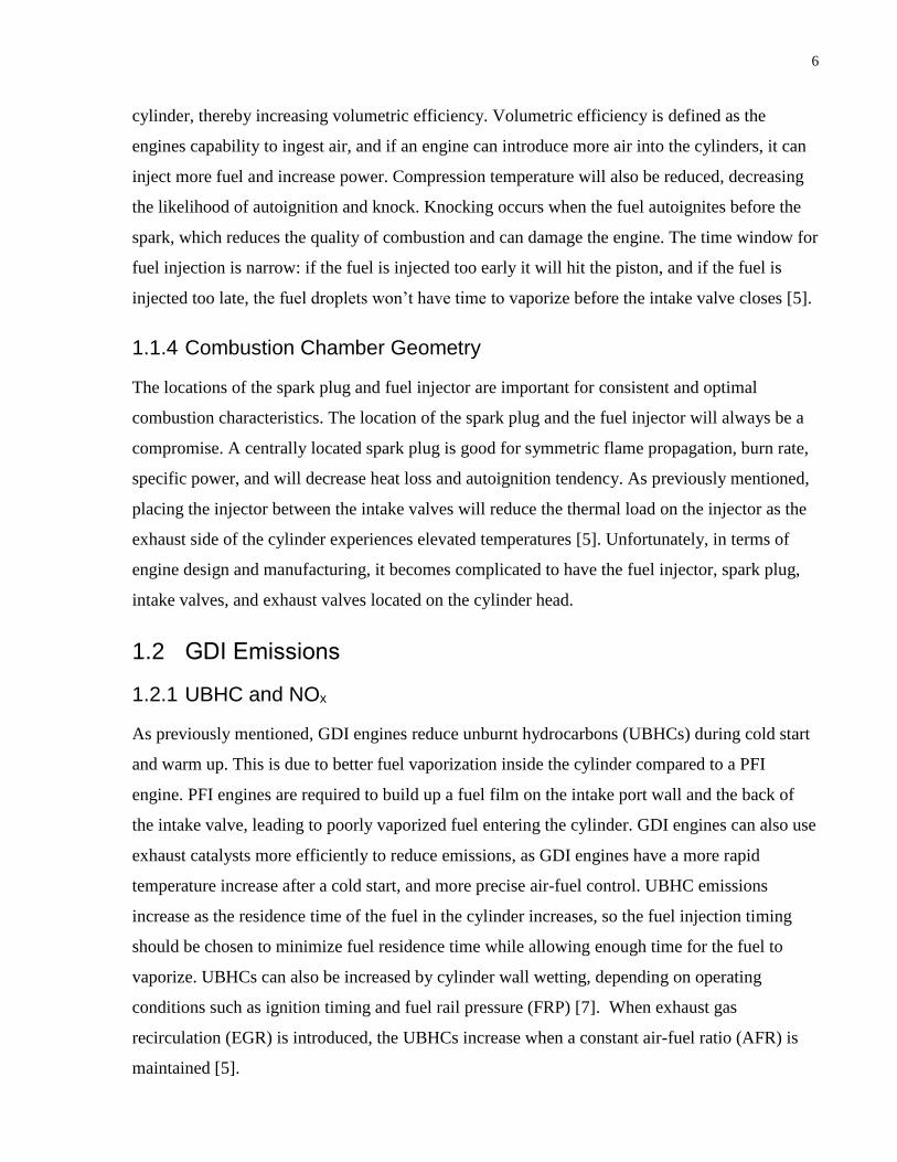
6

cylinder, thereby increasing volumetric efficiency. Volumetric efficiency is defined as the

engines capability to ingest air, and if an engine can introduce more air into the cylinders, it can

inject more fuel and increase power. Compression temperature will also be reduced, decreasing

the likelihood of autoignition and knock. Knocking occurs when the fuel autoignites before the

spark, which reduces the quality of combustion and can damage the engine. The time window for

fuel injection is narrow: if the fuel is injected too early it will hit the piston, and if the fuel is

injected too late, the fuel droplets won’t have time to vaporize before the intake valve closes [5].

1.1.4 Combustion Chamber Geometry

The locations of the spark plug and fuel injector are important for consistent and optimal

combustion characteristics. The location of the spark plug and the fuel injector will always be a

compromise. A centrally located spark plug is good for symmetric flame propagation, burn rate,

specific power, and will decrease heat loss and autoignition tendency. As previously mentioned,

placing the injector between the intake valves will reduce the thermal load on the injector as the

exhaust side of the cylinder experiences elevated temperatures [5]. Unfortunately, in terms of

engine design and manufacturing, it becomes complicated to have the fuel injector, spark plug,

intake valves, and exhaust valves located on the cylinder head.

1.2 GDI Emissions

1.2.1 UBHC and NOx

As previously mentioned, GDI engines reduce unburnt hydrocarbons (UBHCs) during cold start

and warm up. This is due to better fuel vaporization inside the cylinder compared to a PFI

engine. PFI engines are required to build up a fuel film on the intake port wall and the back of

the intake valve, leading to poorly vaporized fuel entering the cylinder. GDI engines can also use

exhaust catalysts more efficiently to reduce emissions, as GDI engines have a more rapid

temperature increase after a cold start, and more precise air-fuel control. UBHC emissions

increase as the residence time of the fuel in the cylinder increases, so the fuel injection timing

should be chosen to minimize fuel residence time while allowing enough time for the fuel to

vaporize. UBHCs can also be increased by cylinder wall wetting, depending on operating

conditions such as ignition timing and fuel rail pressure (FRP) [7]. When exhaust gas

recirculation (EGR) is introduced, the UBHCs increase when a constant air-fuel ratio (AFR) is

maintained [5].

7

NOx increases as the in-cylinder temperature increases. GDI engines will produce more NOx than

PFI engines at idle, due to locally stoichiometric combustion and the associated high heat

release. When EGR is introduced to a GDI engine, it will reduce NOx due to the reduced peak

combustion temperature. However, EGR can result in elevated intake air temperatures which will

reduce engine performance. As with any SI engine, there will always be a compromise between

NOx, UBHCs, and fuel consumption [5].

1.2.2 Particulate Matter

PM describes all substances (other than water) present in the exhaust, in either liquid or solid

phase. Solid PM normally consists of carbon and is commonly referred to as soot.

PFI engines have not generally been concerned with PM emissions, as they do not emit high

enough PM quantities to consider its importance. However, it has been found that GDI engines

produce significantly high quantities of PM emissions, and regulations must be put in place. PM

can result from two types of rich combustion: locally rich air-fuel mixture combustion, and

diffusion burning of incompletely volatilized liquid fuel deposits. PM emissions are often

recorded as the PM mass and the particle number (PN) concentration [5].

1.2.3 Emission Control Systems

Due to increasingly stringent emissions regulations, there must be systems in place to control the

emissions of UBHC, NOx, and PM. Three-way catalysts (TWC) are commonly used in gasoline

engines and are used to reduce NOx, UBHC, and CO emissions in the exhaust stream. TWC’s

have been used successfully with PFI engines for many years. TWC’s are now being used with

GDI engines, but are not designed to control PM emissions. Gasoline particulate filters (GPF) are

an emerging downstream solution to GDI PM emissions, and function similarly to diesel

particulate filters (DPFs). Further information regarding GPFs can be found in Appendix A -

Additional Information. There are also a number of engine operating conditions that can effect

PM emissions that will be discussed further in Chapter 2.

8

1.3 Particulate Matter

1.3.1 Formation

There are 3 modes that describe particulate size distribution:

1. Nucleation mode: particles with a diameter less than 50 nm. Nuclei are formed during

combustion and dilution.

2. Accumulation mode: particles having diameters in the range 50 to 1000 nm.

Accumulation mode particles are typically an agglomeration of nuclei and may also

contain condensed volatiles.

3. Coarse mode: particles having a diameter greater than 1000nm. In engines, these form

from deposits on the cylinder walls and intake/exhaust valves that leave the surface. In

diffusion flames, the coarse mode forms from continued agglomeration and

fragmentation.

All of these modes can be seen in Figure 1.1.4, where the nucleation mode particles form at the

base of the flame, accumulation mode particles form in the middle, and coarse mode particles

form at the top.

Figure 1.1.4: Soot formation, condensation, and oxidation in a diffusion flame [8].

9

In general, PM currently present in engine exhaust is composed of two types of particles:

elemental carbon particles (EC) and organic carbon particles (OC). These small organic particles

are an issue because they make up a large part of urban air particles and are toxic to both people

and the environment [9].

1.3.2 Health Effects

Traffic derived pollutants have been associated with decreased lung function and increased

airway inflammation [10, 11, 12]. While diesel exposure effects have been researched

extensively, exposure to gasoline PM has not, and the chemical composition and volatility of

gases in GDI exhaust are not well known. There are low-volatility gas-phase organics (such as

polycyclic aromatic hydrocarbons (PAHs)) that may condense onto the surface of GDI exhaust

PM [13]. These PAHs tend to have a high risk of adverse health effects, and are often found in

the ultrafine particles that make up a significant portion of the PN concentration emissions [14].

Zimmerman measured PAHs from a wall-guided GDI engine at cold start and highway cruise.

She found that PAH emissions were approximately 10 times higher for cold start then highway,

indicating increased condensation at colder conditions [13].

Lin et al. [14] measured particles roadside in a city in Taiwan, and determined the concentrations

of different particle sizes, as well as which PAHs are present in these particles. Concentrations of

total-PAHs measured in each particle size range went from fine>ultrafine>nano>coarse, but the

mean content (µg-PAH/g particle mass) went from nano>ultrafine>fine>coarse. This provides

further cause for concern about traffic related nano- and ultrafine particles due to the quantity of

these particles emitted. Cytotoxicity response is defined as a reduction in cell viability (RCV)

induced by particles containing PAHs. Nanoparticles displayed the highest cytotoxicity, and the

smaller particles inhibit phagocytic* activity more than coarser particles [14]. More research is

necessary to understand the cytotoxicity of traffic-related particles.

While the inflammatory and cytotoxic characteristics of the nanoparticles is evident, it is

unknown whether the inhaled nanoparticles could translocate from the lung to the circulation in

humans and contribute to cardiovascular disease. Miller et al. [15] investigated the translocation

* Cells that ingest harmful particles.

10

of gold nanoparticles* in human subjects. The authors discovered that the inhaled gold

nanoparticles translocated from the lungs into the blood circulation, indicating that combustion

produced nanoparticles can contribute to cardiovascular diseases [15]. The process itself was size

dependent, as there was greater build-up of smaller nanoparticles. Moreover, the process

occurred rapidly, with gold detected 15 minutes after injection, and still detectable up to 3

months later [15].

The results presented by Zimmerman [13], Lin et al. [14], and Miller et al. [15], all suggest

causes for concern in terms of GDI engine emissions, and are a significant factor in the

increasingly stringent emissions standards. The next chapter will review the effectiveness of both

engine operating conditions and downstream emissions controls reducing total emissions,

focusing specifically on reducing the most dangerous emissions for public and environmental

health.

* Chosen due to gold’s unreactive nature.

11

Chapter 2

Literature Survey

2.1 PM Formation and Morphology

2.1.1 Soot Formation in a Diffusion Flame

As discussed earlier, PM emissions may be harmful to both human and environmental health.

Diffusion burning of fuel rich zones and liquid droplets is a large source of PM emissions.

Maricq [16] discussed the stages of soot formation in diffusion flames: soot inception, surface

growth and agglomeration, oxidation, and soot release. Gasoline containing various amounts of

ethanol (E0 to E85) was studied using a laboratory diffusion flame. The first two features are

present in all the mixtures, while complete soot oxidation is only present in the E85 flame, and

soot release is only present in the E0-E50 flames [16]. In Figure 2.1, the four flames can be seen,

and for all flames except for E85, it is possible to see the soot being formed low in the flame.

The particles are then heated up and becoming luminous, and finally some of the soot is oxidized

before the rest is emitted to the atmosphere.

Figure 2.1: Diffusion flames with varying ethanol content [16].

While ethanol is not used in the current experiments, the tests conducted by Maricq illustrate the

stages of soot formation and the strong impact of fuel composition on that formation. Fuel rich

regions often exist in GDI engines due to the relatively low amount of time for fuel-air mixing.

12

These regions exhibit soot formation characteristics similar to diffusion flames. Similarly, fuel

pooling on a cylinder wall or piston surface (from impingement during fuel injection) burns as a

diffusion flame. Thus, fuel composition is expected to have a significant effect on PM emissions

from GDI engines, and will be discussed further in Section 2.3.

2.1.2 Direct Injection Soot Formation

Since it has been found that GDI engines have particle mass emissions an order of magnitude

higher than PFI engines, and particle number emissions around a factor of 20 higher, there has

been increased research around the formation of soot in gasoline direct injection engines [17]. As

GDI exhaust has not been extensively researched, diesel is a reasonable comparison in terms of

PM emissions. Hesterberg et al. [10] presented a historical overview of the carcinogenic

potential of diesel exhaust in humans, and found results to be inconsistent. However, in 2012 this

was refuted, as the World Health Organization (WHO) declared diesel exhaust to be

carcinogenic [12], and GDI exhaust is likely the same.

Sgro et al. [9] studied the origin of nuclei particles in GDI exhaust and found that a “solid core”

of sub 5nm non-volatile particles form in the combustion chamber at the flame temperature, in

addition to volatile and semi-volatile hydrocarbons. As these particles exit the combustion

chamber and enter the exhaust stream, the organic species will condense or adsorb onto the solid

core particles depending on the dilution ratio*. In terms of dilution ratio, the lower the dilution

ratio is, the more significant the amount of condensation [9]. Maricq determined that secondary

aerosol formation occurs when chemical compounds are oxidized in the atmosphere, decreasing

their vapour pressure and making them more likely to partition to the particle phase, through

condensation or nucleation [18]. These chemical compounds are often PAHs, which are

dangerous when adsorbed or condensed onto nanoparticles [14].

Zimmerman [13] evaluated GDI emissions throughout different seasons in an urban

environment, at different roadside distances, and compared them to the Toronto fleet and

laboratory averages. A 2013 Ford Focus was used both in the lab and on the road at different

* Ratio of ambient air to exhaust stream.

13

engine conditions*. The results showed that volatile organic compounds (VOCs) and PN varied

seasonally, while NOx, CO, and black carbon (BC) did not. Combined PN concentration

emission factors (EFs) were inversely correlated with outdoor air temperature. Cold ambient

temperatures may increase gas-to-particle partitioning of low volatility gases and elongate the

cold start condition. In addition, during the winter the volatility of the fuel is increased to help

with cold starts. Summer ended up having higher EFs than spring, possibly due to the seasonal

changes in fuel formulation. In summer, the volatility is reduced by increasing aromatic content

which is shown to increase soot formation. Evidence of increased aromatic content in the fuel is

provided by measured increases in VOCs and toluene levels in the exhaust in the summer [13].

GDI PN EFs showed spatial variability as measurements taken 15m from the road showed an

average of up to 200% larger EFs than measurements taken 1.5m from the roadway. This effect

is highest in winter and lower in summer due to temperature – less condensation occurs at higher

temperatures, an effect which was not seen in the PFI vehicle [13]. This indicates that

condensation plays an important role in the evolution of GDI PM emissions in the atmosphere.

The condensation sink was similar in the background aerosol and the near-road (15m) condition,

suggesting that small particle growth is due to gas-particle portioning of low volatility organic

vapours within the plume, as opposed to existing organics in the urban air [13].

2.2 GDI Engine Effects and PM

While aftertreatment devices are seen as the most effective way to reduce PM emissions, it is

also possible to optimize the engine operating parameters to reduce emissions. In this section,

different engine operating parameters will be studied for their effects on PM mass and PN

concentration emissions.

2.2.1 Piston Wetting

Direct injection engines have increased cylinder wall and piston head fuel wetting compared to

PFI engines. Moreover, they may have in-cylinder temperatures that are too low for the oxidation

of hydrocarbons late in the expansion stroke and during exhaust. This can cause increases in

UBHC and PM emissions. Warey et al. [19] ran laboratory tests on a GDI engine to test the

* This is the same engine used in this investigation.

14

effects of different fuels on wall wetting. The effects of fuel composition will be discussed later.

Warey et al. found that the effect of piston wetting on PM emissions was directly related to fuel

injection, as both particle size and mass increased during fuel injection. PFI engines were tested

using the same amount of fuel and did not show the same correlation. It was also found that the

amount of fuel injected did not affect the mean particle size, but did increase mass loading by

70% [19].

Furthermore, Fatouraie et al. [20] used an optically accessible GDI engine to examine the effects

of ethanol on PM emissions. They took images of the combustion chamber through the cylinder

wall, as they found that a window in the piston crown significantly affects soot formation, due to

changes in the thermal conductivity and surface-fuel interactions on the piston head. Due to the

low rate of heat transfer, the optical piston had a much higher surface temperature, which

resulted in higher vaporization of the fuel and significantly lower soot formation. Therefore, the

piston temperature and ability for the fuel to evaporate from the piston head is important to the

production of PM emissions [20].

2.2.2 Injector Pressure and Charge Motion Effects

An increase in GDI injector pressure was initially necessary for turbocharging, to overcome

higher in-cylinder pressures; however, it has since become essential due to the need for better

atomization and mixing of the fuel. This increase can provide better combustion and reduce

emissions, which is especially important with tougher regulations in the near future. For

homogeneous GDI engines, the main sources of emissions during hot operation are mixture

inhomogeneity, fuel pooling, and the “injector tip diffusion flame” phenomenon. This

phenomenon occurs when fuel absorbs into the tip deposit layer during fuel injection, and then

releases after injection stops, resulting in incomplete combustion after the normal flame

propagation. The optimal tumble charge motion* is high for homogenous combustion, as it leads

to better spray vaporization and charge homogeneity.

Piock et al. [21] used a single cylinder GDI engine in a lab to look at the effect of these

parameters on PM emissions at different fuel pressures, injector specifications, and charge

* Method by which fuel-air mixing is achieved. The movement of the charge within the cylinder.

15

motion cases. It was found that increasing the fuel pressure decreases both PM mass and PN

concentration. This occurs due to improved atomization and mixture preparation, as well as a

reduction of the “injector tip diffusion flame” effect. The biggest effect of tumble charge motion

enhancement are low levels of PM mass and PN emissions. Piock et al. [21] used different

injectors while varying the number of plumes and fuel flow to measure the effect on PM mass

emissions. It was found that the fuel pressure effect predominates the effects of charge motion

and injector design. The injector specification does make a difference, but tends to be negligible

compared to fuel pressure and charge motion. Finally, it was also determined that higher fuel

pressure reduces the effect of the injector tip diffusion flame [21].

Wang et al. [22] performed similar tests on a single cylinder, spray-guided, research GDI engine.

They varied the injection pressure and found that high injection pressures improve PM mass

emissions due to better spray atomization. At high injection pressures, PN concentration

emissions can increase from an increased rate HC particle nucleation [22]. These results agree

with the results found by Piock et al. [21]. Wang et al. [22] also tested the effect ethanol had on

fuel pressure, and it was discovered that ethanol produced much lower PM mass emissions than

gasoline, due to its oxygen content and higher volatility. PN concentrations were higher, as

ethanol promotes particle nucleation instead of condensation or adsorption.

2.2.3 Injector Fouling

Wang et al. [22] also investigated the effect of injector fouling on PM emissions. They used three

injectors: one clean, and two fouled injectors with different amounts of carbon build-up. It was

identified that using gasoline with higher carbon build-up led to a decrease in flow rate and

higher PM emissions. This was likely due to increased fuel impingement and fuel pooling,

resulting in diffusion combustion and high HC and soot formation. This could also be due to

gasoline being adsorbed on carbon deposits near the injector tip, which contributes to diffusive

combustion after the main combustion [22]. When ethanol was used, it was found that there was

still fuel impingement and injector fouling; however, ethanol evaporates easily, leading to less

diffusion combustion and lower HC and soot formation [22].

2.2.4 Injection Timing and Strategies

Significant soot formation is caused by fuel droplets pooling on the piston surface and

subsequently burning in a diffusion flame. Injection timing is an important parameter for GDI

16

engines as early injection can provide sufficient time for fuel evaporation prior to ignition. Seong

et al. [23] studied the effect of injection timing on a 4-cylinder GDI engine in a lab, and found

that there is a trade-off for injection timing. If the injection is advanced too far there will be

increased fuel impingement on the cylinder wall and piston head. The emissions were minimized

at an injection timing of 260° before top dead centre (BTDC), while injection timings of 330

°BTDC and 190 °BTDC had increased PM emissions due to reduced time for fuel-air mixing and

vaporization, and increased fuel impingement, respectively [23]. Similar results were obtained by

Jiao et al. [24] who used computational fluid dynamics (CFD) to model the effect of injection

timing on soot emissions. Retarding injection timing (Start of Injection (SOI) =330, 320, 290

°BTDC) resulted in decreasing PM emissions, due to a reduction of fuel impingement as the

timing is retarded. For the range of injection times tested by Jiao et al., the amount of fuel film

on the wall at the time of spark ignition correlates well with the PM emissions, as they both

decrease with retarding of the SOI timing [24]. These results agree with those obtained by Seong

et al. However, Seong et al. [23] also tested further retardation of fuel injection timing, and their

results continue to show this trend until a point, after 260 °BTDC, where there is not enough

time for good fuel-air mixing and vaporization.

In terms of PM morphology, Seong et al. [23] discovered that small nanoparticles were more

present at the retarded fuel injection timing compared to other conditions. These particles were

mostly 9-25 nm in diameter; however, it was observed that a number of sub-10 nm particles were

produced as well. These small nanoparticles were observed at a slightly decreased rate in other

injection strategies, as they were being attached to sub- 25 nm particles [23]. Furthermore, He et

al. [25] found that advanced fuel timing resulted in the formation of large particles, and the PN

concentration emissions were dominated by the accumulation mode particles. Furthermore, not

only does early SOI timing increase PN concentration, but it also shifts the peak particle size

larger, which can also significantly increase the PM mass emissions [25].

There are the two main injection strategies that were briefly discussed in the introduction: wall-

guided and spray-guided. Both have their own respective advantages and disadvantages. Wall-

guided generally injects the fuel from the side of the cylinder, and uses the piston head geometry

and in-cylinder airflows for fuel-air mixing and to direct the mixture towards the spark plug. This

method increases fuel consumption, PM, HC, and CO emissions as the fuel does not completely

evaporate from the piston surface [26]. In contrast, spray-guided generally injects the fuel from

17

the cylinder head, and directs some of the plumes toward the spark plug and the rest into the

cylinder. Spray-guided theoretically has the highest efficiency; however, there are disadvantages.

The spray-guided technique reduces PM emissions by avoiding significant wall wetting, and

increases fuel efficiency, but can also increase the rate of injector fouling [26]. Wang et al.

looked more in-depth at the types of particles these injection methods were creating. Wall-guided

produced mostly EC, likely due to increased levels of fuel impingement and pooling, similar to

diesels. Spray-guided displayed the opposite effect, and produced mostly volatile organic

materials, with EC only accounting for 2-29% of all PM emissions [22]. It is important to

remember that these numbers do not include total PM emissions. Volatile organic materials are

more dangerous, so there is a trade-off between having less total particulate matter, or

minimizing the amount of volatile and semi-volatile particles that lead to more negative health

effects.

2.2.5 Valve and Spark Timing

Transient operation of a GDI engine tends to produce the most emissions, so Tan et al. [27] ran

experiments on a Jaguar spark ignited (SI)/homogeneous charge compression ignition (HCCI)

research engine with variable valve timing (VVT). Different intake valve opening (IVO) timings

were tested and had similar PN concentration and PM masses, indicating that IVO has little

influence during transient operation. For varied exhaust valve closing (EVC), PN concentrations

were slightly lower at an EVC of 15 ⁰after top dead centre (ATDC) than when EVC was 30

⁰ATDC or TDC, while PM mass was fairly constant.

Spark timing, however, had a large effect on emissions. A spark timing of 30 ⁰BTDC had the

lowest PN concentrations and PM mass, as well as the highest efficiency. Particle emissions

increased as spark timing was retarded, and was highest at 15 ⁰BTDC due to incomplete

combustion. However, at 35 ⁰BTDC, there was little time for fuel-air mixing prior to

combustion, and the low exhaust temperature decreased the vaporization of injected fuel. This

led to the poor combustion and increased PM emissions [27].

Seong et al. [23] performed Transmission Electron Microscopy (TEM) analysis to look at the

effect of spark timing on soot production and morphology. They discovered that extremely

advanced ignition timing would leave some fuel on the cylinder wall and piston head until late in

the compression stroke. This led to poor combustion characteristics, as there was not enough

18

fuel-air mixing at low temperatures. These conditions were very similar to those at late injection.

Short vaporization time and fuel wetting of surfaces caused increased nucleation at extremely

retarded and advanced timings. Currently the literature has contradictory results of primary

particle size and soot mass emissions. However, primary particle size could increase from the

coalescence of two particles, and low temperatures could quench particle growth, so it is

assumed that the increasing trend for advancing injection timing reflects complex soot formation

processes in GDI engines [23]. It should be noted that the high magnification of the TEM

analysis can transform particles, and this can affect the TEM results.

2.2.6 Air-Fuel Ratio

As mentioned above, transient operation of a GDI engine tends to produce the most emissions.

During these transient periods it can be difficult for the engine control unit (ECU) to maintain

stoichiometric combustion. Tan et al. [27] performed tests on a Jaguar SI/HCCI research engine

to study this phenomenon. Since the main engine control parameters remained constant, the

transient performance was only affected by the amount of intake air and fuel being injected.

During transient operation, the air-fuel ratio peaked at a maximum of 1.2 (fuel lean), due to a

delay in the fuel injection response based on an oxygen sensor in the exhaust. The intake air

response was rapid due to fast-response sensors. The AFR control could not ensure

stoichiometric combustion at all times during transient operation [27].

In general, particle emissions increased drastically during transient operation in both nucleation

and accumulation modes. The overall increase of PM emissions showed a strong correlation with

rich combustion [27].

2.2.7 Engine Coolant Temperature

The coolant temperature used around the combustion chamber controls the thermal boundary

condition of the engine. Both the engine coolant temperature (ECT) and the residual combustion

heat significantly affected the spray characteristics and fuel impingement, which directly affects

PM emissions. Fatouraie et al. [7] used a direct injection spark ignition (DISI) single cylinder

optical engine to look at the effect of ethanol on fuel spray and impingement as a function of

ECT. Fuels with a fuel rail pressure (FRP) of 100 bar and SOI of 250 °BTDC were tested at 25

°C and 90 °C. For E0 fuel, the temperature increase caused flash boiling of the volatiles,

resulting in increased rates of vaporization. The increased rate of vaporization of the fuel also

19

resulted in narrower plume angles and higher fuel impingement due to the collapse of the

individual plumes [7].

Serras-Pereira et al. [6] also studied the effect of ECT on spray development and impingement

using an optical DISI engine at high and low ECTs: 90 °C and 20 °C, respectively. The engine

operating temperature can have significant effects on fuel spray formation in DISI engines,

specifically affecting the quality of charge preparation due to the reduced mixing times. At 90

°C, the gasoline spray is affected in terms of initial shape and development. In Figure 2.2,

plumes 2, 3, 4, and 5 all collapsed towards the centre of the chamber, and all spray penetrations

were reduced due to the increased evaporation. This behavior was not seen at the 20°C condition.

Figure 2.2: Schematic of a spray-guided injector system [6].

Serras-Pereira et al. [6] also discovered, using heat flux detectors, that the higher ECT caused a

drastic reduction in gasoline impingement. The temperature increase caused plumes 1 and 6 to

widen and break up more rapidly, and initiated the collapse of plumes 2-5 towards the centre of

the cylinder. In addition, the initial gasoline spray tip penetration is reduced [6]. This observation

was also found by Chen at al. [28], who found that a warm engine has a shorter fuel spray due to

increased vaporization and spray atomization. This resulted in lower PN concentrations

compared to a cold engine [28]. These results somewhat oppose those found by Fatouraie et al.

[7]. While all the studies found that the plumes collapsed and vaporization was increased for

higher ECTs, Fatouraie et al. [7] discovered that increased ECT resulted in higher fuel

impingement.. This is likely due to the studies having different engine operating parameters and

20

fuel injection strategies. For example, they used different FRPs with Serra-Pereira et al. [6] using

a FRP of 150 bar compared to a FRP of 100 bar for Fatouraie et al. [7]. They also used different

SOIs, using 280 ° and 250 °BTDC respectively. Furthermore, Serras-Pereira et al. used a spray-

guided GDI engine, while Fatouraie et al. used a wall-guided engine. As mentioned in Section

2.2.4, the two different fuel injection strategies can have significant effects on the PM emissions

produced, and would likely contribute to the increased wall impingement seen by Fatouraie et al.

[6, 7].

Spray impingement was determined to be the dominant factor in soot formation. The higher

sensitivity of E0 to ECT for both fuel spray and soot formation indicates spray characteristics are

more important in soot formation than fuel chemistry. The ECT effects on in-nozzle flow can

also influence spray features. At 25⁰C the earliest impingement on the cylinder liner is in its first

half, while at 90⁰C the narrower plume caused the impingement to be physically lower on the

liner [7]. The study done by Fatouraie et al. [7] did not explicitly look at PM emissions, but

instead looked at the spray characteristics that will influence emissions. Jiao et al. [24] used their

CFD model to look at the effect of temperature on PM emissions in GDI engines. Two cases

were used: one at low temperature and one at high temperature. The soot emissions for the low

temperature case were two orders of magnitude higher than those for the high temperature case.

The high temperature case also had decreased fuel film on the wall due to the higher wall

temperature [24]. This result agrees with the hypothesis that most PM emissions from a GDI

engine occur during the cold-start phase.

2.3 Fuel Composition and PM

The fuel composition used in GDI engines can have a large effect on PM emissions. This is

because PM emissions can be correlated with the fuel properties. Therefore, it is possible to

predict PM emissions from the physical and chemical properties of fuel.

2.3.1 Ethanol/Gasoline Blends

Renewable energy sources are currently a large research focus due to the increasing rate of

global warming and the depletion of conventional oil reservoirs. Ethanol is a promising

renewable source for vehicles as it can be produced entirely from organic materials. Ethanol is

currently being used as a gasoline additive to improve combustion and for the perceived

21

reduction of GHG emissions. Ethanol reduces PM emissions in diesel engines due to the oxygen

atoms present in the fuel oxidizing the soot, but tests with GDI engines have less definitive

results.

Chen et al. [28] tested a variety of fuels (n-octane, isooctane, xylene, and ethanol) at a

stoichiometric fuel-air ratio using a single cylinder, optical access, spray-guided direct injection

engine. They found that increasing the ethanol content results in longer spray durations, lower

mixture homogeneity, increased combustion duration and variability, and an increase of PM

emissions [28]. It was shown in a previous study that at rich conditions with high PM emissions,

adding ethanol can reduce the PM emissions due to the oxygen in the fuel increasing soot

oxidation [28]. Fatouraie et al. [7] also examined the effect of ethanol content in a DISI wall-

guided research engine and found results that agree with Chen et al. [28]. The PM emissions

increased from E0 to E50 to E100, which indicates that higher ethanol contents result in less

complete combustion. The spray plumes for the fuels had similar penetration distances, but E0

displayed a wider plume angle with the angle decreasing with increased ethanol content. The

opposite was found to be true for wall impingement which was lowest for E0. E100 had the

fastest fuel vaporization even though it has the highest enthalpy of vaporization. This is likely

due to the heavy compounds of gasoline taking longer to vaporize [7]. Similarly, He et al. [25]

found that ethanol can have significant effects on PM emissions, depending on the injection

timing. If there is fuel impingement on the piston, ethanol’s high heat of vaporization slows the

evaporation process, leading to a less homogeneous mixture near the piston, or even pool fires.

This produces higher PN concentrations. However, if there is no impingement, the oxygen in

ethanol reduces the total PN concentrations by suppressing the soot formation [25].

On the contrary, Munoz et al. [29] found that increasing ethanol content resulted in significant

decreases in PN for a GDI engine. They found that increasing ethanol from E0 to E10 to E85

reduced both PN concentrations and PAHs, which were most pronounced at transient conditions.

They found that the difference between E0 and E10 was much larger than the difference between

E10 and E85, indicating that large ethanol contents may not be needed. As noted above, there are

contradicting studies on the effects of ethanol addition, likely due to different engine parameters

affecting fuel impingement and pooling [29]. Maricq et al. [30] varied ethanol content from 0-

50% in a wall-guided GDI engine, and found similar results that both PM mass and PN

concentration decreased with increasing ethanol content, ~30% and ~45% over the range,

22

respectively. In addition, Maricq et al. found that HC were decreasing with ethanol content, but

advised that ethanol changes the HC composition. This might increase alcohols and aldehydes

which are under-represented by the FID, so the results may not be significant [30]. Furthemore,

in terms of a diffusion flame it was found by Maricq [16] that increasing ethanol strongly

reduces the amount of semi-volatile organics and nucleation mode particles. However, this only

occurred at high concentrations of ethanol, in this case an E85 blend (85% ethanol) [16]. In most

cases of gasoline/ethanol blends, the concentration of ethanol is not high enough for this to

occur.

Chan et al. [31] tested the differences between using E0 and E10 fuels on the road at different

driving conditions. It was seen that for a GDI stock engine, using E10 decreased PN

concentrations for the U.S. Federal Test Procedure 75 (FTP-75), but increased PN concentrations

for the US06 Supplemental Federal Test Procedure (US06) [31]. This is likely because the US06

cycle is more demanding and the engine was more likely to be running on homogeneous charge,

where the longer vaporization time and fuel needed can result in increased impingement and

higher PM emissions. The operating conditions of an engine can have a significant effect on the

engine combustion, so it is the difficult to produce a definitive answer on the effectiveness of

ethanol blending.

2.3.2 PM Index and PN Index

Components with characteristics such as high boiling points, low vapour pressures, and high

aromatic content tend to produce higher PM emissions. Aromatic content can be represented by

the double bond equivalent (DBE) value. Two research groups, one at Honda and the other at the

University of Oxford, have developed a single number index to convey the propensity of fuel to

produce PM emissions. Both the Honda PM Index (index to predict PM mass emissions based on

weight fraction, vapour pressure, and DBE value of each fuel component) and Oxford PN Index

(index to predict PN by modifying Raoult’s law into the PM model) have shown good

correlation between the PM emissions and the physical and chemical properties.

The original PM Index was developed for PFI engines by Aikawa et al. [32], which accurately

predicts potential PM mass and number based on fuel composition, using the DBE values and

vapour pressures of each component. The PM Index has subsequently been applied to GDI

engines. The significant effects observed by changing vapour pressure further suggest that fuel

23

impingement and the subsequent diffusion burning is a key aspect of GDI engines PM emissions.

Since GDI engines are not premixed, the longer vaporization times of low vapour pressure

components will not only lead to higher impingement, but also more fuel rich regions, leading to

higher PM emissions. The equation developed for the PM Index can be seen below in Equation

2.1.

Aikawa et al. [32]:

𝑃𝑀 𝐼𝑛𝑑𝑒𝑥 = ∑ 𝐼[443𝐾]𝑛𝑖=1 = ∑ (

𝐷𝐵𝐸𝑖+1

𝑉.𝑃(443𝐾)𝑖× 𝑊𝑡𝑖)

𝑛𝑖=1 (2.1)

where:

I – fuel component

DBE – double bond equivalent

V.P – vapour pressure

Wt – mass fraction.

While the PM Index is accurate, it requires a full detailed hydrocarbon analysis using gas

chromatography that is both complicated and expensive. Each of the components is introduced to

the equation individually; however, in reality the vapour pressure of each component in a blend

does not act as a combination of the values. Leach et al. [33] adapted the PM Index to make it

simpler to calculate for blended fuels. The new index, named the PN Index, was introduced to

simplify the process. Instead of using mass fractions, the PN Index uses volume fraction as that

is the industry standard for blended fuels. In addition, the Dry Vapour Pressure Equivalent

(DVPE), otherwise known as the Reid Vapour Pressure (RVP) was used, as it is the European

standard measurement. The equation for the PN Index can be seen below in Equation 2.2.

24

Leach et al. [33]:

PN Index =∑ [𝐷𝐵𝐸𝑖+1]𝑉𝑖

ni=1

DVPE (kPa) (2.2)

where:

DBE – double bond equivalent

Vi – volume fraction

DVPE – dry vapour pressure equivalent.

The indices created by Aikawa et al. [32] and Leach et al. [33] both had excellent predictions for

PM emissions; however, the PN Index was shown to be slightly more accurate for GDI engines

[33].

2.3.3 Other Fuel Blends

The issue with these indices is that they lack information on individual fuel components. Fuel

blends can be complicated, as different components within the fuel react with each other to

produce emissions and this can be hard to measure. Chen et al. [34] decided to link individual

fuel components to PM emissions using a mixture Design of Experiment (DoE) and a spray-

guided turbocharged GDI engine. The DoE test measured particle number concentrations for

both the nucleation and accumulation mode of particle growth, which depend only on relative

proportions of fuel components. The test fuels were formed from n-octane, isooctane, xylene,

and ethanol, and each fuel had a RON of between 90 and 100. Xylene tended to produce the

most particles as it is an aromatic hydrocarbon, and acted as a soot precursor, which promoted

particle formation. It was also found that n-octane reduces accumulation mode particles, likely

due to promoting the oxidation reaction [34].

The large increase of PM emissions due to aromatic compounds can be explained by PM

emissions’ correlation with DBE values and higher boiling points. Karavalakis et al. [35]

investigated the impact of gasoline aromatic content on tailpipe emissions from SIDI vehicles,

and found that at equivalent carbon numbers, aromatics will produce higher PM emissions than

paraffins due to their higher boiling point. In addition, fuels with equivalent aromatic content

will produce different quantities of PM emissions. Even though two fuels have equivalent

25

aromatic content, the fuel that consists of components with higher boiling points resulted in

increased PM emissions. The results gained by Karavalakis et al. were further validation of the

PM Index [35].

As mentioned earlier, Warey et al. [19] tested a variety of fuels to see their effects on piston

wetting. They used a laboratory GDI engine, and tested gasoline, n-pentane, iso-octane, toluene,

and n-undecane. These fuels were chosen due to the variety in their molecular structures and/or

the variety in their volatility. Toluene and n-pentane produced the highest PM size and mass.

This is likely due to toluene being an aromatic compound, thereby making it likely to form PAHs

which are soot precursors. This effect is likely due to their individual molecular structure and not

their volatilities, as toluene and iso-octane have similar boiling temperatures [19].

2.3.4 Pentane Fuel Blends

In general, heavier fuel components (high carbon number, high boiling points, low vapour

pressures, and high DBE values) produce increased PM emissions. Leach et al. [36] examined

the effect of low boiling point (light-end) components on the fuel spray inside a GDI engine.

Light-end components have not been associated with the production of an increasing number of

particles, but during their research, they found that n-pentane, a light-end component, is essential

in order to reflect real-world evaporation behaviour. Due to its high volatility, the pentane breaks

up the spray earlier after it enters the cylinder, which causes the mixture to be less homogeneous.

Blended fuels without pentane were tested, and it was found that PN emissions decreased with

decreasing vapour pressure. To confirm their results, they demonstrated that the fuels with

pentane reflected the PN Index, while the fuels without pentane did not [36].

Moreover, Warey et al. [19] found that n-pentane surprisingly produced higher PM emissions

than n-undecane even though it has a higher volatility, which means it should theoretically

evaporate faster. The reason it does not evaporate faster is because n-pentane has a boiling point

much less than the surface temperature. This can cause surface boiling of the fuel films, which

reduces evaporation from the cylinder wall and piston head because a vapour layer forms

beneath the fuel film and acts as insulation. On the other hand, n-undecane’s boiling temperature

is high enough to avoid this and it vaporizes more quickly. Thus, the difference between the

paraffins was due to volatility differences [19].

26

2.4 Previous Work

The results of previous research investigating this GDI engine showed significant variability in

the PN concentration during steady-state tests. Ramos [37] found that the temperature and

humidity of the dilution air provided to the rotating disk thermodiluter was inconsistent, and the

instrument was sensitive to these changes. To account for this, a dry dilution air supply was

installed for the rotating disk thermodiluter, which led to a significant reduction in test-to-test

variability. In terms of steady-state variability, Ramos also examined: fuel temperature; engine

deposits and engine cleaning; crankcase oil intake; and oil temperature and age. All of these

parameters were found to have little effect on the steady-state variability [37].

Furthermore, Ramos investigated the effect of fuel composition on PM emissions, and found that

changes to fuel composition can significantly alter PM emissions. His research focused on the

effect of ethanol due to the government mandate on at least 5% ethanol content in gasoline, and

he also studied the effect of aromatic content in gasoline. In Figure 2.3, the results of his research

can be seen. Ramos found that the standard error of the average PN concentration measurements

increased with both ethanol and toluene content, indicating that fuel composition can

significantly affect the variability of the PM emissions. In addition, while it was hypothesized

that increasing the aromatic content, e.g. toluene in this investigation, would increase the PN

concentration; however, in Figure 2.3 it can be seen that this is not the case. Ramos found that

the PN concentration seemed to be affected by a combination of both ethanol and toluene. This is

likely because ethanol has a slow rate of vaporization relative to the heavy components in

gasoline, which can also slow down the vaporization of the other components, leading to fuel

rich cores producing increased PM emissions [37, 25].

27

Figure 2.3: Two-minute average PN concentrations for each test group of the different fuel

blends. Shaded areas indicate standard error [37].

Rais [MASc Thesis in Progress] extended this research by re-creating gasoline using pure blends,

initially consisting of 65% isooctane and 35% toluene by volume. This blend was chosen as

isooctane is the simplest surrogate for gasoline, and toluene was a cost-effective method to

replicate the aromatic content of gasoline. Prior to Rais, Ramos [37] found that gasoline itself

had a large effect on PM emissions and there was a lot of variability between different gasolines.

For this reason, Rais removed the ethanol content to focus on the effect of varying fuel

composition of gasoline: it is difficult to examine the impact of ethanol when the impact of

gasoline is not known [MASc Thesis in Progress].

The base 65% isooctane and 35% toluene blend produced PN concentrations more than an order

of magnitude less than those from Shell 91 pump gasoline. In later blends, Rais introduced

gasoline additives, trimethylbenzene, and oil in an attempt to produce emissions similar to those

of gasoline; however, when none of these blends worked, hexane, xylene, naphthalene, sulphur,

and two heavy solvents were added to the base blend. While this final blend produced

significantly higher PM emissions compared to the base blend, they were still over an order of

magnitude lower than those of gasoline [MASc Thesis in Progress].

28

2.5 Experimental Goals

The goal of this thesis is to determine the source of the emissions gap between gasoline and the

pure fuel blends. Future blends will be based upon previous blends tested by Rais and current

literature. The original matrix created by Rais was initially based upon a paper by Leach et al.

[36], then was updated and edited using the Shell 91 pump gasoline fuel analysis report, which

was not available when Rais began testing [MASc Thesis in Progress]. Using this information

will provide a better understanding of the components, or combination of components, that are

producing large amounts of PM emissions. Apart from ascertaining the source of the emissions

gap, there will also be a more general investigation into the effect of fuel composition on PM

emissions.

29

Chapter 3

Experimental Set-up

This chapter will focus on the physical apparatus used in this investigation. Figure 3.1 illustrates

the experimental set-up of the engine and its associated controls, the exhaust line and sampling

tube, and all the analyzers with their associated heated lines, filters, and diluters. Several changes

were made between the research conducted by Ramos [37] and Mireault [38]; however, not

many changes have been made since the research done by Ramos. As a result, the experimental

set-up used by Ramos [37] has been repeated verbatim in this thesis. All repeated material will

be denoted by italics in order to clearly define material attributable to Ramos.

Figure 3.1: Research engine and emissions sampling arrangement [37].

3.1 Research Engine

The engine used in this research is a pre-production four-cylinder GDI engine used in the 2012

and newer Ford Focus. It employs side mounted, wall-guided direct injectors and is naturally

aspirated. Table 3.1 lists some of the major specifications of the engine. A stock ECU—known as

a Powertrain Control Module (PCM) with Ford—electronically controls the operation of the

engine, and in production vehicles the transmission and other drivetrain components. It has the

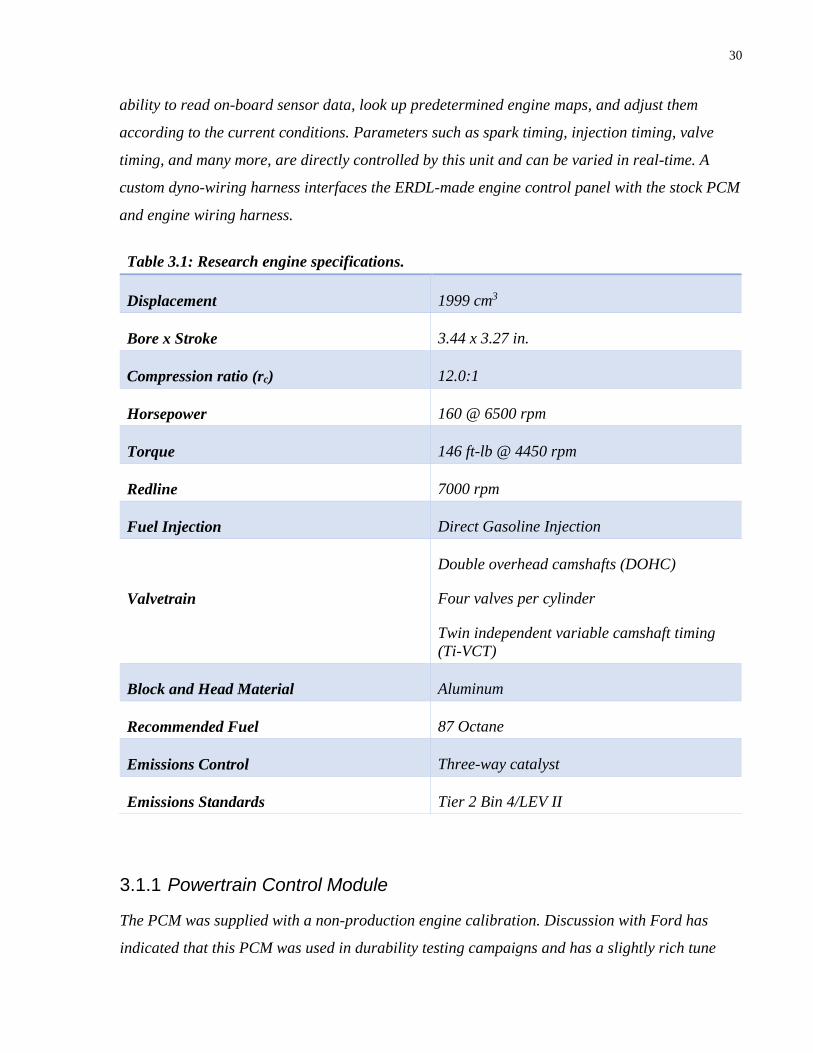
30

ability to read on-board sensor data, look up predetermined engine maps, and adjust them

according to the current conditions. Parameters such as spark timing, injection timing, valve

timing, and many more, are directly controlled by this unit and can be varied in real-time. A

custom dyno-wiring harness interfaces the ERDL-made engine control panel with the stock PCM

and engine wiring harness.

Table 3.1: Research engine specifications.

Displacement 1999 cm3

Bore x Stroke 3.44 x 3.27 in.

Compression ratio (rc) 12.0:1

Horsepower 160 @ 6500 rpm

Torque 146 ft-lb @ 4450 rpm

Redline 7000 rpm

Fuel Injection Direct Gasoline Injection

Valvetrain

Double overhead camshafts (DOHC)

Four valves per cylinder

Twin independent variable camshaft timing

(Ti-VCT)

Block and Head Material Aluminum

Recommended Fuel 87 Octane

Emissions Control Three-way catalyst

Emissions Standards Tier 2 Bin 4/LEV II

3.1.1 Powertrain Control Module

The PCM was supplied with a non-production engine calibration. Discussion with Ford has

indicated that this PCM was used in durability testing campaigns and has a slightly rich tune

31

and is not configured for proper catalyst function. Indeed, wide-band oxygen sensor readings

showed a fuel-air equivalence ratio of approximately 1.015 at steady conditions. However, the

exact calibration of the PCM is not known and it is currently unmodifiable.

3.1.2 Engine Exhaust System

A standard equipment exhaust manifold was used in this set-up, which normally has an

incorporated TWC—see Figure 3.1. However, given that the PCM is not configured to run with a

TWC, the exhaust manifold was modified to remove the stock exhaust after-treatment. This was

accomplished by cutting open the catalyst can, removing the catalytic core and re-welding the

can back together. Keeping an otherwise stock exhaust manifold will permit future work on this

engine to look at catalyzed vs. uncatalyzed emissions under an identical set-up. The exhaust

manifold was joined to the exhaust tube, which in turn feeds the raw engine exhaust to the

sampling tube at a typical tail-pipe distance. The exhaust system and sampling tube were

designed in accordance to US EPA guidelines [39].

3.1.3 Fueling System

A custom fuel system was implemented here, as the use of a stock fuel system would not be

appropriate. Figure 3.2 shows a schematic diagram of the fueling system. Two fuel tanks hold

the test fuel and are selected via two three-way solenoid valves, which control the flow path of

the outgoing and return fuel. A coarse filter removes large debris from the flow to protect the

low pressure fuel pump, while a fine filter is employed to prevent any smaller debris from

entering the high pressure loop on the engine side. A pressure regulator ensures that fuel at 55

psi is continuously supplied to the high pressure fuel pump, with unused fuel being returned to

the appropriate tank. A fuel cooler was added in this investigation to control the fuel

temperature being fed to the high pressure loop. The fuel temperature is measured at the exit of

the pressure regulator before the fine filter.

32

Figure 3.2: Fueling system flow diagram [37].

The addition of the fuel cooler was done by Ramos in order to more precisely control the

temperature of the fuel entering the engine, as the fuel temperature was found to be steadily

increasing through the duration of the test [37]. The design can be seen in Figure 3.3. The fuel

cooler is a single shell, single tube, heat exchanger using building water to cool the fuel. There is

a ball valve at the entrance of the fuel cooler which allows the user to turn the water on or off

completely, while there is a precision needle valve at the outlet for accurate control of the water

flow [37].

Figure 3.3: Cross-sectional view of the fuel cooler. Blue arrows indicate heat exchanger

water and red arrows indicate fuel [37].

33

3.1.4 Dynamometer

A GO-Power D-557 water brake dynamometer was used to apply a load on the engine. The

water brake dynamometer works by transferring the mechanical energy of the engine to the

water due to friction and turbulence generated between the rotor and stator. The rotor is coupled

to the engine, while the stator is coupled to the dynamometer stand. A strain gauge measures the

force applied to the stator by the rotating fluid in the internal cavity. Water is supplied at a

pressure that is regulated down from building pressure; the amount of water flowing to the

dynamometer is controlled via the dynamometer controller (see Section 3.2.2).

3.1.5 Oil Cooler

A sandwich type oil cooler from a 2012 Ford Focus ST (turbocharged, high performance variant

of this research engine) was installed for this work. Figure 3.4 shows the installation location

and the relevant flow paths. The oil cooler works by flowing engine coolant through a heat

exchanger that is seated above the oil filter. Pressurized oil is forced through this cooler before

continuing through the filter and back to the engine block. The oil cooler was installed in the

typical coolant loop location for the heater core on a production vehicle. This location ensures

that coolant flows through the oil cooler at all times while the engine is turning over because the

coolant path for the heater core is unobstructed by the thermostat. By having coolant flowing at

all times, the cooler works to both heat the oil more quickly in cold conditions and cool the oil

when the engine is fully warmed. A ball valve downstream of the oil cooler allows disabling of

the unit by preventing coolant flow to it.

34

Figure 3.4: Schematic of oil cooler. Note: oil flow paths do not intersect.

3.1.6 Crankcase Ventilation Filter

The research engine design used in these experiments was designed with a positive crankcase

ventilation (PCV) system. This system uses the engine to create a vacuum in the intake manifold

to draw the crankcase air and blow-by gases (products of combustion and unburned fuels that

pass by the piston into the crankcase) back into the intake stream so that they can be combusted

with the incoming fuel-air mixture. This is done to reduce the amount of uncontrolled gases

emitted to the atmosphere. The research engine has an oil separator to ensure that no crankcase

oil is ingested into the induction system; however, this system was found to be ineffective, so a

MANN+HUMMEL ProVent200 oil separator filter was installed upstream of the intake

manifold [37]. In Figure 3.5 an exploded view of the filter can be seen, and its main purpose is to

absorb all liquid oil and oil vapours.

35

Figure 3.5: Exploded view of the MANN+HUMMEL ProVent200 oil seperator filter [37].

3.2 Engine Controls

A custom made engine control panel operates the major electrical control functions for the

engine. These include the starting system, the fueling system, the PCM system, and the

emergency stop system. The control panel is the same one used in the first study on this engine

by Mireault [38]; specific details are omitted here for the sake of brevity.

3.2.1 Throttle Control

An ECM appsCAN throttle pedal simulator was used to simulate the throttle pedal signals to the

PCM. Modern vehicles make use of throttle-by-wire systems, where an electrical sensor

measures the throttle position at the pedal and relays that to the PCM. The PCM then performs

the necessary calculations to select the appropriate throttle plate angle given the commanded

throttle position and other critical parameters; the PCM physically controls the throttle plate

angle with a servo motor. As owner safety is of utmost importance to auto manufacturers, the

throttle pedal actually has two sensors that must mathematically correspond to each other; the

PCM reads both values and should one not correspond to the other a fault is triggered and the

vehicle enters what is known as “limp-mode”. Therefore, the coordination of these two signals is

necessary for proper engine operation. The appsCAN provides a synchronous output of signals

in a stand-alone fashion required to operate the throttle [40].

36

Specific to this research engine, the throttle pedal outputs two position signals, APPS1 and

APPS2, based on its current position to the PCM. Measurement of the signals showed that

APPS2 is 50% of APPS1 at any given position. As such, the appsCAN module was set to run in

ratiometric mode, where the two desired outputs would run at a fixed percentage of an input

voltage signal. A 0-10 V input signal from the NI DAQ (see Section 3.3.1) was used to control

the appsCAN which in turn provided two signals at 50% and 25% of the original input. Note that

the signal was scaled in the Labview program to fit the required signal range of the pedal to a 0-

100% scale (i.e. a 0 % selection in the program would yield a 1.6 V output to the module, which

corresponds to the 0% pedal position for sensors APPS1 and APPS2). Further logic was

incorporated to read throttle ramps from a file, as well as provide for certain fail safes.

3.2.2 Dynamometer Control

A Digalog 1022A Dyno Controller was used to provide control of the water brake dynamometer

mentioned in Section 3.1.4. The dyno controller reads engine speed from a magnetic pick up on

the dynamometer, as well as the strain voltage (calibrated for torque loading) from the strain

gauge. The dyno controller has the ability to control the load and speed set-points given these

two readings by controlling the amount of water entering the dynamometer through a

compressed air controlled water valve. Essentially, this works by regulating the amount of

compressed air supplied to open the water control valve. This is done with an on-board closed

loop PID controller, which was re-calibrated along with the stain-gauge prior to start of this

work. In this investigation, the controller was set to control the engine speed, the set-point of

which was controlled by analog voltage signals from the NI DAQ (see Section 3.3.1).

3.3 Engine Data Acquisition and Control

Critical engine parameters, temperatures, and pressures were recorded using two independent

data acquisition systems. Engine specific parameters were recorded using the high-speed

controller area network (CAN) bus that is standard to production vehicles and known as the on-

board diagnostic version 2 (OBD-II). The other acquisition unit—a National Instruments

CompactDAQ—measured temperatures, pressures, and other analog signals, as well as

outputted control signals.

37

The data stream collected during this research project was recorded using a Labview program

created by Mireault [38], and updated by Ramos [37].

3.3.1 National Instruments Compact DAQ

A National Instruments (NI) CompactDAQ (cDAQ-9174) populated with four modules captured

analog data such as temperature, pressure, and load. Two NI-9211 thermocouple modules

provided acquisition of temperature data, while an NI-9205 module collected analog sensor

data. A single NI-9263 module handled analog outputs used to control the throttle simulator

(Section 3.2.1) and the dyno controller (Section 3.2.2) for the load and speed set-points,

respectively. Table 3.2 lists all the sensor data collected and the analog outputs controlled by the

DAQ. All thermocouples used were Omega K-Type grounded thermocouples (HGKQSS-18G-

12). Pressure measurements were made with engine manifold air pressure sensors (MSD

Ignition 2312).

Two independent LabVIEW programs were used with the DAQ for data recording and output

control. The main program for recording purposes is a modified version of the original program

used by Mireault [38]. The above inputs from the NI DAQ, as well as inputs from the standard

emissions bench (Section 3.5.3) over TCP/IP, are read and written to a file at 5Hz and 1Hz,

respectively. Modifications to this program include the addition of the previously excluded

emissions analyzers and the calculation of corrected emissions from the standard emissions

bench. The second program controls the throttle (load) and engine speed set-points for the

throttle and dyno controllers, respectively. Manual control or pre-developed load and speed

ramps are available for selection by the user.

38

Table 3.2: Inputs and outputs from NI DAQ. Units shown are appropriately scaled from

analog voltages and currents.

NI Module Recorded/Outputted Parameter

Inputs

9211 (2)

TC1 – Exh. Temperature (°C) TC2 – Exh. Temperature (°C)

TC3 – Exh. Temperature (°C) TC4 – Exh. Temperature (°C)

Ambient Air Temperature (°C) TSI Diluter Head Temperature (°C)

Oil Temperature (°C) Fuel Temperature (°C)

9205

Abs. Ambient Pressure (kPa) Abs. Exh. Pressure (kPa)

Engine Speed (rpm) Engine Load (ft-lb)

Fuel-Air Equivalence Ratio (Φ) Engine Speed Set-Point (rpm)

Outputs 9263 Throttle Position (%) Engine Speed Set-point (rpm)

3.3.2 OBD-II

Data from the OBD-II CAN bus was gathered using a generic after-market OBD-II reader. The

reader contains an ELM-327 chip which is widely used to decode CAN messages over the OBD-

II protocol— known as parameter IDs (PIDs)—and interface with computer software via USB.

As the OBD-II standard is made to provide a minimal level of access to diagnose issues with

vehicles, this chip can only decode those CAN values deemed essential for troubleshooting by

regulatory agencies. However, manufacturers do employ proprietary CAN messages which are

only decodable with proprietary readers. A list of the available PIDs recorded during this

investigation is provided in Table 3.3.

39

Table 3.3: PIDs recorded from OBD-II data stream.

Engine Speed (rpm) Engine Coolant Temperature (°C)

Intake Air Temperature (°C) Calculated Load (%)

Air Flow Rate (g/s) Ignition Timing Advance (°)

Accelerator Pedal Position (%) Absolute Throttle Position (%)

Fuel Rail Pressure (kPa) Air-Fuel Equivalence Ratio (λ)

Long Term Fuel Trim (%) Short Term Fuel Trim (%)

3.4 Particulate Matter Sampling

The following section will detail the particulate matter sampling apparatus used in this

investigation. The two dilution systems are discussed first, followed by the instruments used to

analyze size, mass, and composition of the particles. All referenced instruments were serviced at

acceptable intervals prior to and during data collection per manufacturer recommendations.

3.4.1 TSI Rotating Disk Thermodiluter and Thermal Conditioner

A TSI 379020A Rotating Disk Thermodiluter supplied diluted exhaust gas to the particle sizer

used in this study (see Section 4.5.4). The 379020A is controlled and fed dilution air from a

combination of a TSI 379030 Thermal Conditioner Air Supply and a Matter Engineering MD19-

3E Raw Gas Diluter; this latter unit will henceforth be referred to as the ‘diluter box’. This

diluter is capable of achieving DRs ranging between 15:1 to 3300:1 at flow rates between 0.5-20

lpm [41]. The 10-cavity rotating disk mixes fixed volumes of exhaust gas with the primary

dilution air [68]. The par-diluted sample is sent to a thermal conditioner, before being cooled by

the secondary dilution [41]. Through results obtained by Mireault, the diluter was found to

produce stable DRs; however, true DRs were found to be consistently under the set-point desired

[38]. As a result, the true dilution ratio was measured using CO2 as a tracer gas.

40

In previous work done by Ramos, it was found that the dilution air humidity was affecting the

variability in PM emissions [37]. Thus, the HEPA filters located inside the thermodiluter were

connected to dry pressurized air, which was supplied at ambient pressures by venting any excess

air to the atmosphere.

3.4.2 Dekati FPS 4000 Diluter

The Dekati Fine Particle Sampler (FPS) 4000 provided diluted exhaust sample for the filter

collection cart (Section 3.4.5). The unit is capable of supplying 60-160 lpm of diluted sample at

DRs of 20-200 [42]. The Dekati incorporates two stages of dilution to achieve the desired

dilution ratio. The first stage of dilution occurs through a perforated tube, where the dilution air

is drawn into the sample stream through a porous metal tube; the second stage is an ejector type

diluter [42]. The DR is controlled by the amount of dilution air flowed, which the unit controls

via several solenoid valves and critical orifices [42]. A primary dilution air heater and a dilution

probe heater allow for adequate DT control. A calculated dilution ratio is provided by on-line

measurement of temperature and pressures through the system, though its accuracy has been put

into question by previous work at the ERDL [38, 43, 44]. Therefore, as with the rotating disk

thermodiluter, the true dilution ratio was measured using CO2 as a tracer gas

3.4.3 Dry Air Supply

Dry dilution air was supplied to both the Dekati diluter and the rotating disk thermodiluter via a

system of filters and desiccant driers on the building’s pressurized airline. This dry air supply

meets or exceeds the specifications required by the Dekati. This dry air supply was also used to

provide the dry air needed for the emissions bench (HFID and HCLD analyzers)—see Section

3.5.3.

3.4.4 Engine Exhaust Particle Sizer

A TSI 3090 Engine Exhaust Particle Sizer (EEPS) provided total PN concentrations and particle

size distribution characterizations of the engine exhaust. Particles are characterized by their

electrical mobility in 32 discrete bin sizes from 5.6 to 560 nm [45]. The EEPS works by charging

incoming exhaust particles to a known level with a corona charger [45]. The charged particles

then flow through the column with a centrally mounted, positively charged electrode repelling

the particles radially where the electrometers are located. The electrometer that any given

41

particle impacts is related to its electrical mobility and therefore, its particle size. These

electrometers measure the charge of the impacted particle allowing both size and concentration

data to be extracted simultaneously [45]. Data was logged using the proprietary TSI software at

a rate of 2Hz. The EEPS measured diluted exhaust from the aforementioned TSI Rotating Disk

Diluter (Section 4.3.2).

3.4.5 PM Filter Collection Cart

An ERDL designed and built filter collection cart was used in this study to collect PM laden

filters for gravimetric and compositional analyses. Figure 3.6 shows a schematic configuration

of the filter collection cart. Diluted exhaust sample is drawn through the filter cart via two

vacuum pumps—one for each filter cassette holder. A cyclone removes particles greater than 10

µm upstream of the filter holders, which hold the filter cassettes that collect the PM on each

filter. Sample collection is controlled by two three-way solenoid valves, which when selected to

sample connect the exhaust flow path through the filter cassette holders.

Figure 3.6: Filter cart flow diagram. Dashed lines indicate flow path in "bypass" mode [37].

The filter cart used in this research has been previously used by many students [37, 38, 43, 44];

however, the filter cart went through some modifications after Mireault [38]. Prior to the

modifications, the system was experiencing pressure spikes whenever the solenoids were

switched to sample, as the system was sensitive to back-pressure. To alleviate this issue, a bypass

section was connected so that the filter cart pumps would run continuously regardless if the

solenoid was set to sample or not. To protect the mass flow controllers from particles, a Parker-

Balston 58N Engine Exhaust Filter (with a 100-12-404 filter element) was installed in the bypass

stream. In addition, a custom heater (Neptech Inc. Hot Pocket custom heater blanket) was

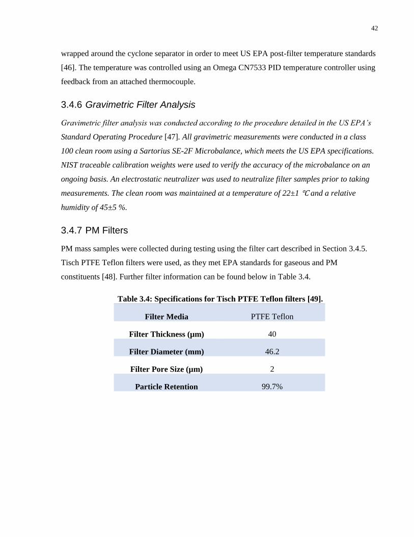
42

wrapped around the cyclone separator in order to meet US EPA post-filter temperature standards

[46]. The temperature was controlled using an Omega CN7533 PID temperature controller using

feedback from an attached thermocouple.

3.4.6 Gravimetric Filter Analysis

Gravimetric filter analysis was conducted according to the procedure detailed in the US EPA’s

Standard Operating Procedure [47]. All gravimetric measurements were conducted in a class

100 clean room using a Sartorius SE-2F Microbalance, which meets the US EPA specifications.

NIST traceable calibration weights were used to verify the accuracy of the microbalance on an

ongoing basis. An electrostatic neutralizer was used to neutralize filter samples prior to taking

measurements. The clean room was maintained at a temperature of 22±1 ℃ and a relative

humidity of 45±5 %.

3.4.7 PM Filters

PM mass samples were collected during testing using the filter cart described in Section 3.4.5.

Tisch PTFE Teflon filters were used, as they met EPA standards for gaseous and PM

constituents [48]. Further filter information can be found below in Table 3.4.

Table 3.4: Specifications for Tisch PTFE Teflon filters [49].

Filter Media PTFE Teflon

Filter Thickness (µm) 40

Filter Diameter (mm) 46.2

Filter Pore Size (µm) 2

Particle Retention 99.7%

43

3.5 Gaseous Sampling

The following section discusses the four instruments used for gaseous sampling in this

investigation. An FTIR provided gaseous speciation, while a standard emissions bench gave

regulated emissions concentrations. A small CO2 monitor was used to measure dilution ratios of

the two diluters and an AFR sensor provided corrected fuel-air equivalence ratios for the fuel

used. Figure 3.1 shows the arrangement of the equipment used.

3.5.1 Fuel-Air Equivalence Ratio

The research engine is nominally equipped with a wide-band oxygen sensor that provides the

PCM with a reading of the AFR for closed loop control. However, an additional, highly accurate

and stand-alone AFR sensor system was employed to gather independent AFR data from the

exhaust stream. This was done with an ECM 2400E-1 wide-band oxygen sensor in conjunction

with an ECM AFRecorder 2400 to provide real-time AFR data. The main benefit of this system is

that the AFRecorder can be configured for different fuel compositions in order to display a

corrected AFR reading [50].

3.5.2 FTIR

An MKS 2030HS Fourier Transform Infrared Spectroscopy (FTIR) was used to perform gaseous

speciation of the exhaust gas in real time. Raw exhaust is drawn from the sample tube through a

heated filter that removes exhaust particles from the sample stream. A heated sample line carries

the remaining gas phase species to the FTIR analyzer. Both the heated filter and the heated

sample line were operated at 191 ℃. Data was recorded using the MKS supplied FTIR software

at 2 Hz. The software permits the off-line reprocessing of spectral data for different “recipes”—

pre-selected lists of compounds for analysis.

The FTIR operates on an infrared light absorption measurement technique, not dissimilar to

Non-Dispersive Infrared emissions analyzers. They differ, however, in the number of gaseous

species they are capable of analyzing; where an emission analyzer is typically limited to a single

compound (single wavelength), an FTIR can analyze any compound that falls within its

spectrum. In this case, the FTIR operates in the mid-infrared region of 2-20 µm and any

compound that absorbs infrared radiation in this region can be measured [51]. An interference

pattern is passed through the gas sample and the resulting light is measured and converted to an

44

absorbance spectrum using Fast Fourier Transform mathematics [51]. Using reference files for

pure species, the instrument deconstructs the spectrum based on a preselected batch of species

assumed to be in the sample; known as the ‘recipe’. The development of the recipe is of utmost

importance to the operation of the instrument. Including compounds not present in the sample,

or conversely, excluding compounds actually present, will result in erroneous readings. The

FTIR recipe used in this investigation is detailed in Section 4.2.1.

3.5.3 Standard Emissions Bench

An emissions bench measured raw exhaust concentrations of the standard (regulated) emissions.

These include total hydrocarbons (THC), oxides of nitrogen (NOx), carbon dioxide (CO2),

oxygen (O2), and carbon monoxide (CO). Data was logged using the Labview program through

the TCP/IP protocol; a network switch connected all four analyzers to the logging computer.

Table 3.5 summarizes the analyzers including the ranges used and their respective calibration

cylinders. All analyzers were zeroed with emissions grade nitrogen (N2). The four analyzers were

made by California Analytical Instruments (CAI) and they each conform to US EPA guidelines

for measuring their respective species. The same dry air supply used for the aforementioned

diluters was also used for the emissions bench (Section 3.4.3)

The exhaust sample is drawn in through the sample probe at the heated filter head. A filter

removes particles from the exhaust stream while maintaining the sample temperature at 180 ℃.

A heated 3/8 in. Teflon sample line carries the exhaust sample to the emissions bench from the

heated filter, where it is teed off to the different analyzers. The two heated analyzers (THC and

NOx) have internal sample pumps which pull the sample through their respective heated sample

lines (each set to 149 ℃). The two unheated analyzers (CO2/O2 and CO) use an external sample

pump which passes the sample through two chillers to remove water (a source of interference in

these analyzers). A calibration flow drawer controls the flow of calibration and sample gases to

the probe; the exact calibration method is described in Section 4.2.2.

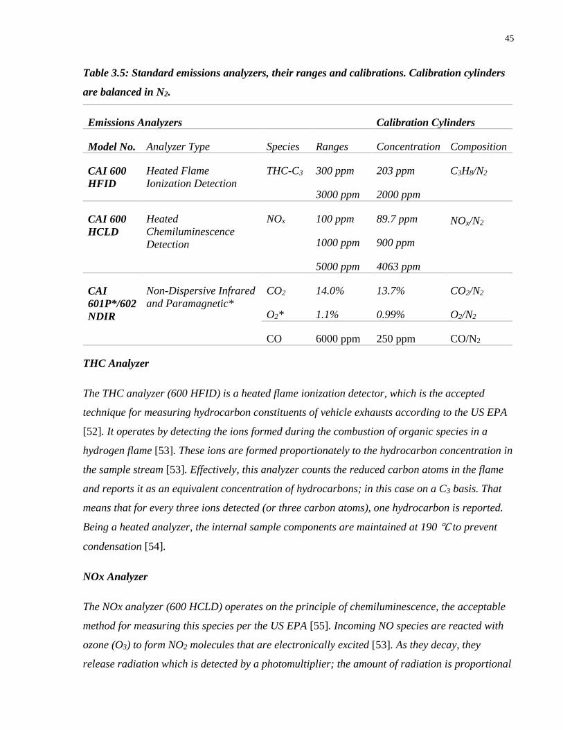
45

Table 3.5: Standard emissions analyzers, their ranges and calibrations. Calibration cylinders

are balanced in N2.

Emissions Analyzers Calibration Cylinders

Model No. Analyzer Type Species Ranges Concentration Composition

CAI 600

HFID

Heated Flame

Ionization Detection

THC-C3 300 ppm

3000 ppm

203 ppm

2000 ppm

C3H8/N2

CAI 600

HCLD

Heated

Chemiluminescence

Detection

NOx 100 ppm

1000 ppm

5000 ppm

89.7 ppm

900 ppm

4063 ppm

NOx/N2

CAI

601P*/602

NDIR

Non-Dispersive Infrared

and Paramagnetic*

CO2

O2*

14.0%

1.1%

13.7%

0.99%

CO2/N2

O2/N2

CO 6000 ppm 250 ppm CO/N2

THC Analyzer

The THC analyzer (600 HFID) is a heated flame ionization detector, which is the accepted

technique for measuring hydrocarbon constituents of vehicle exhausts according to the US EPA

[52]. It operates by detecting the ions formed during the combustion of organic species in a

hydrogen flame [53]. These ions are formed proportionately to the hydrocarbon concentration in

the sample stream [53]. Effectively, this analyzer counts the reduced carbon atoms in the flame

and reports it as an equivalent concentration of hydrocarbons; in this case on a C3 basis. That

means that for every three ions detected (or three carbon atoms), one hydrocarbon is reported.

Being a heated analyzer, the internal sample components are maintained at 190 ℃ to prevent

condensation [54].

NOx Analyzer

The NOx analyzer (600 HCLD) operates on the principle of chemiluminescence, the acceptable

method for measuring this species per the US EPA [55]. Incoming NO species are reacted with

ozone (O3) to form NO2 molecules that are electronically excited [53]. As they decay, they

release radiation which is detected by a photomultiplier; the amount of radiation is proportional

46

to the amount of NO in the sample [53]. This instrument also has the capability to convert the

NO2 in the exhaust to NO by decomposition, before being reacted with the ozone. The reported

concentration in this configuration, as used in this investigation, is therefore NOx (NO + NO2).

The internal temperature of components in contact with sample gas are maintained above 68 ℃

[55].

CO2/O2 and CO Analyzers

Two unheated analyzers were used for the remaining three gases of the emissions bench: 601P

NDIR for CO2/O2 and 602 NDIR for CO. Both analyzers operate on the principle of non-

dispersive infrared analysis, with the CO2 analyzer having an optional paramagnetic analyzer

for O2. These are both accepted practices for measuring these species according to the US EPA

[56, 57] The NDIR analyzer operates on the principle of infrared absorption where the radiation

absorbed in a sample cell is compared to a reference cell [53]. Radiation not absorbed by the

exhaust sample is absorbed by one side of the detector, while the radiation not absorbed by the

reference gas is absorbed by the other side [53]. Different amounts of absorption in the two

halves causes’ diaphragm distention from the resulting difference in pressure [53]. A microflow

detector measures the induced flow between the two halves, which is converted to species

concentration using the calibration as a reference [58]. As water causes a large interference in

the infrared spectrum for the above compounds, it must be removed from the sample before

being analyzed (see Section 4.2.2).

3.5.4 Mini CO2 Monitor

A LI-COR LI-840A CO2/H2O analyzer (CO2 monitor) was used to measure diluted CO2

concentrations to calculate true dilution ratios of the two diluters. The CO2 monitor operates on

the principle of NDIR [59], just as the analyzer in the emissions bench does. A small sample

pump draws the diluted exhaust stream to the analyzer through 1/4 in. Teflon tubing. The unit

incorporates a water sensor that corrects the CO2 reading for water interference [59], so no

chiller is necessary.

47

3.6 Test Fuels

3.6.1 Shell 91 Pump Gasoline

The test fuels used in this study were informed by analysis of Shell 91 pump gasoline,

specifically chosen because it was the only available pump gasoline with zero ethanol content.

This is permitted according to the Renewable Fuels Regulations, which states that the total

gasoline pool for a supplier must contain 5% ethanol [60]. Accordingly, the supplier can have no

ethanol in their 91 octane fuel, and higher ethanol levels in their 87 and 89 octane fuels as long

as the total ethanol content is over 5%. In previous work on this engine, the effect of ethanol

was studied [37]. In this study, ethanol was removed to allow other fuel composition effects to be

researched without the influence of ethanol.

3.6.2 Gasoline Compositional Report

Since Shell 91 pump gasoline was the base fuel for this study, it is important to know the exact

volume composition of the gasoline. A gas chromatogram was done on a Shell 91 pump gasoline

sample to determine the volume, mass, and molar compositions [61]. In Table 3.6 and Table 3.7,

the Shell 91 pump gasoline composition can be seen by component group and carbon number

respectively [61].

Table 3.6: Shell 91 pump gasoline composition by component group.

Group %Wgt %Vol %Mol

Aromatics 50.168 43.765 46.291

I-Paraffins 29.583 33.423 30.155

Naphthenes 3.424 3.414 3.598

Olefins 5.696 6.360 6.724

Paraffins 10.084 12.022 12.497

Oxygenates 0.027 0.026 0.057

Unidentified 1.017 0.988 0.678

48

Table 3.7: Shell 91 pump gasoline composition by carbon number.

Carbon # %Wgt %Vol %Mol

C2 0.027 0.026 0.057

C3 0.016 0.024 0.035

C4 1.977 2.586 3.257

C5 14.907 17.886 19.757

C6 11.451 12.688 12.818

C7 27.746 25.618 28.178

C8 24.923 23.986 21.783

C9 12.307 11.179 9.615

C10 3.760 3.338 2.649

C11 1.591 1.428 1.016

C12 0.267 0.245 0.154

C13 0.009 0.009 0.004

The fuel blends were created using the volume content of Shell 91 pump gasoline, in order to

create a simple, accurate, surrogate*. The test fuels were created with similar aromatic content

due to the contribution of aromatics as soot precursors [34]. The test fuels also attempted to

reasonably match the carbon numbers using the base components listed below in Table 3.8. The

two solvents were blends of C9-C10 and C10-C12 aromatics, respectively, and were used due to the

high purchasing cost of pure heavy hydrocarbons. They accounted for the hydrocarbons in the

C9-C12 range. As previously mentioned in Section 2.4, Rais [MASc Thesis in Progress] went as

far as testing Fuel 4, the composition of which can be found in Table 5.1. The theory behind the

choice of that blend can be found in Section 2.4. The following blends in this test were based on

tests done by Rais, the gasoline composition report, and the literature.

* Budget, complexity, and time restraints required the surrogate to be simple.

49

Table 3.8: Components used in test fuels: chemical formulas and specifications.

Component Chemical Formula Specifications

N-pentane C5H12 [62]

Hexane, mixture of isomers C6H14 [63]

Xylenes C8H10 [64]

Toluene C7H8 [65]

2,2,4-Trimethylpentane (isooctane) C8H18 [66]

Thiophene C4H4S [67]

Naphthalene C10H8 [68]

APSOL Solvent #1 (Solvesso 100) C9-C10 aromatics* [69] [70]

APSOL Solvent #2 (Solvesso 150) C10-C12 aromatics [71] [72]

3.6.3 Test Fuels

For this study, several different fuel blends were used to examine the effect of fuel composition

on PM emissions. Table 3.9 lists each test fuel, with their compositions defined by volume

percentage. Due to the complex compositions of the fuels, they have been named by the order in

which they were tested. Refer back to this test matrix, or the identical one in Section 5.1, to

determine the composition of a fuel blend.

* molecular formulas for the two solvents were calculated using benzenes alkyl derivatives: C6H5-(CnH2n+1) [88]

50

Table 3.9: Fuel composition test matrix by volume percentage.

Isooctane Toluene Pentane Hexane Xylene Naphthalene Solvent #1 Solvent #2 Thiophene

Fuel 1 65.00% 35.00% 0.00% 0.00% 0.00% 0.00% 0.00% 0.00% 0.00%

Fuel 2 62.00% 33.00% 5.00% 0.00% 0.00% 0.00% 0.00% 0.00% 0.00%

Fuel 3 55.00% 30.00% 15.00% 0.00% 0.00% 0.00% 0.00% 0.00% 0.00%

Fuel 4 20.31% 19.34% 0.00% 33.85% 14.51% 0.28% 8.22% 3.39% 0.10%

Fuel 5 20.31% 19.34% 19.34% 14.51% 14.51% 0.28% 8.22% 3.39% 0.10%

Fuel 6 20.37% 19.40% 19.40% 14.55% 14.55% 0.00% 8.24% 3.39% 0.10%

Fuel 7 20.39% 19.42% 19.42% 14.56% 14.56% 0.00% 8.25% 3.40% 0.00%

Fuel 8 22.33% 19.42% 19.42% 14.56% 14.56% 0.00% 9.71% 0.00% 0.00%

Fuel 9 29.13% 22.33% 19.42% 14.56% 14.56% 0.00% 0.00% 0.00% 0.00%

Fuel 10 30.00% 35.00% 20.00% 15.00% 0.00% 0.00% 0.00% 0.00% 0.00%

Fuel 11 52.00% 28.00% 20.00% 0.00% 0.00% 0.00% 0.00% 0.00% 0.00%

Fuel 12 52.00% 28.00% 0.00% 20.00% 0.00% 0.00% 0.00% 0.00% 0.00%

In Table 3.10, the paraffinic and aromatic content for each test fuel is shown. While not exact,

the majority of the fuels have similar aromatic and paraffinic contents to the Shell 91 gasoline

analyzed in the gas chromatograph.

Table 3.10: Paraffin and aromatic content for all test fuels.

Paraffins Aromatics

Shell 91 45% 43%

Fuel 1 65% 35%

Fuel 2 67% 33%

Fuel 3 70% 30%

Fuel 4 56% 38.8%

Fuel 5 56% 38.8%

Fuel 6 56% 38.5%

Fuel 7 56% 38.5%

Fuel 8 58% 35%

Fuel 9 65% 38%

Fuel 10 65% 35%

Fuel 11 72% 28%

51

Chapter 4

Experimental Methods

The following chapter will describe the experimental methods used in this study. These methods

and procedures were used during testing to ensure consistency and minimize variability.

Previous procedures used by Rais [MASc thesis in progress], Ramos [37], and Mireault [38]

were re-created in this study to ensure that the data was obtained in a similar manner, and that it

could be compared.

4.1 Engine Testing

4.1.1 Pre-test Setup

At least one hour prior to running, the engine dynamometer controller is turned on to warm up.

During this time, water is supplied to the dynamometer seals and the engine coolant heat

exchanger. Next, the positive crankcase ventilation (PCV) filter is cleaned to avoid oil build-up,

and compressed air is supplied to the water valve controller for the dynamometer. Then, both the

PCM (Powertrain Control Module) and the fuel pump are turned on, and the test fuel is poured

into the fuel tanks.

Following this, the control systems are set up for optimal test control. The OBD-II (on-board

diagnostics) program is connected to the ECU to record the engine outputs. Then, the LabVIEW

DAQ recorder, throttle controller, and ECM AFR meter are turned on in preparation for the test.

The engine is now prepared to run.

4.1.2 Steady-state Testing

After start-up, the engine is run under idling conditions. During this time, the load control is

tested at 5% of the max throttle; this can be seen at around minute 3 in Figure 4.1. In addition,

the functionality of all the engine systems and readings are verified. The engine is switched to

highway conditions (a throttle setting of 24% and a speed of 2600 rpm) once the ECT reaches

and stabilizes at 50 °C, which can be seen after minute 6 in Figure 4.1. The engine is then run

under these conditions for 100 min (Figure 4.2). In Figure 4.2, at around 15 min, it can be seen

that the load drops significantly below 40 ft-lbs. This drop requires a manual increase to open the

52

throttle, which was done using the LabVIEW program and the ECM appsCAN module described

in Section 3.2.1. This phenomenon should be investigated further in the future.

Figure 4.1: Initial engine speed during steady-state tests.

Figure 4.2: Full engine speed and load during steady-state tests.

The ECT and fuel temperature are controlled by varying the flow rate of water through their

respective heat exchangers. If the ECT, engine load, and engine speed are properly maintained,

they should be similar to the desired operating conditions (Table 4.1). In later tests there were

issues with high post-sampling exhaust temperatures; however, the increase in temperature was

0

500

1000

1500

2000

2500

3000

3500

0 1 2 3 4 5 6 7 8 9 10

Spee

d [

rpm

]

Time [min]

0

5

10

15

20

25

30

35

40

45

50

0

500

1000

1500

2000

2500

3000

3500

0 20 40 60 80 100 120

Load

[ft

-lb

]

Spee

d [

rpm

]

Time [min]

Speed

Load

53

shown to have little effect on the PM emissions, and may be an artificial increase due to the

thermocouple drifting. Refer to Appendix B - Potential Sources of Variability for more

information.

Table 4.1: Desired operating conditions at engine highway settings.

Parameter Value

Engine Coolant Temperature (ECT) 90 °C

Oil Temperature 98 °C

Heat Exch. Coolant Temperature 75 °C

Heat Exch. Water Temperature 67 °C

Calculated Load on OBD-II 60%

Torque 41 lb-ft

Post-sampling Exhaust Temperature 320 °C

Fuel Temperature 22.5 °C

After 100 minutes, the engine is ready for shut down. To avoid heavy loading on the engine, the

engine load is slowly ramped down from highway conditions to idle by stepping down the

throttle. Then, the engine is idled for several minutes so that it can cool slowly. When the ECT is

below 60 °C and the oil temperature is below 75 °C, the ECU is switched off to shut down the

engine (Figure 4.2).

4.2 Gaseous Emissions Sampling

The following section outlines the analyzers used to measure the gaseous emissions: the FTIR,

the emissions bench, and the LI-COR.

4.2.1 FTIR

An FTIR was used to provide speciation of the chemical species shown in Table 4.2. The recipe

was the same one used by Ramos [37], who updated the recipe from Mireault [38] to include

ethane and benzene as there were significant concentrations of these components in the exhaust

[37].

54

Table 4.2: Compounds measured by FTIR.

Nitric Oxide (NO) Nitrogen Dioxide (NO2) Propylene (C3H6)

Nitrous Oxide (N2O) Acetylene (C2H2) Benzene (C6H6)

Formaldehyde (CH2O) Carbon Monoxide (CO) Toluene (C7H8)

Methane (CH4) Ethylene (C2H4) Water (H2O)

1,3-Butadiene (C4H6) Acetaldehyde (CH3CHO) Pentane (C5H12)

Carbon Dioxide (CO2) Ethane (C2H6) Isobutylene (C4H8)

To begin the FTIR procedure, a black dewar is filled up with liquid nitrogen. A vent at the

bottom of the dewar is opened, and the dewar is left uncapped until liquid nitrogen begins

flowing out of the vent.

Once the FTIR is warmed up, a diagnostic check is done to make sure that the FTIR is within its

operational tolerances. This is done before every test to prevent instrument drift. After the

diagnostic check, the GDI recipe used by Ramos is loaded, and a new test file is saved [37]. Prior

to testing, a background reading is taken by flowing zero grade nitrogen through the instrument.

The instrument waits in this standby condition until the FTIR is ready to measure.

The FTIR begins sampling once the engine exhaust has reached a temperature of 300 °C. The

high temperature is necessary as the instrument and heaters are sensitive to the exhaust

temperature, and at 300 °C the exhaust is near its steady-state temperature (~320 °C). To begin

sampling, the FTIR sampling section is switched from the purge gas to the raw exhaust, and the

pump is turned on.

Once the sampling has been completed, the FTIR is turned off by switching the pump to off, and

toggling the sample line to the purge gas.

55

4.2.2 Emissions Bench

As mentioned in Section 3.5.3, the emissions bench consists of an HFID, an HCLD, and two

NDIR analyzers (CO2/O2 and CO). The heated filters and sample lines are continuously left on as

they can require multiple hours to heat up. To begin the procedure, the zero air cylinder and the

helifuel (40% hydrogen, 60% helium) cylinder are opened, and the external sample pump for the

two NDIR analyzers is turned on. Following this, the burner in the HFID is ignited using the

helifuel and zero air. Next, all the instruments are set to their measurement modes, which

switches on the internal pumps for the HFID and the HCLD. Prior to calibration, the analyzers

must warm up for at least 30 minutes.

With the analyzers fully warmed up, the calibration procedure can begin. There is a 3-way valve

on the sampling tube, prior to the heated filter, that controls whether the emissions bench

samples calibration gases (or room air), or exhaust gases. This valve is set to calibration prior to

the next steps. Initially, the zero gas N2 cylinder is opened and set to 15 psi. The emissions bench

has a flow drawer that allows quick selection of the gases, and at this time it must be set to zero

gas. While the zero gas N2 is flowing through the analyzers, each of them must be zeroed in

every range. This gives a baseline reading similar to the FTIR background. Next, the ranges for

each analyzer are calibrated by flowing each of the span gases shown in Table 3.5 for each

corresponding range in the analyzer.

Once all the analyzers have been properly calibrated, they are all set to their respective

measurement modes. The 3-way valve on the sampling tube is set to sample the engine exhaust,

and values are recorded using the LabVIEW program described in Section 3.5.3.

After the test has been completed, the 3-way valve at the heated filter is set to sample room air.

The sample pumps continue to run for another 30 minutes to clear all the analyzers of excess

water. After 30 minutes has passed, the helifuel cylinder and zero air cylinder are closed to

extinguish the flame in the HFID analyzer. Finally, all analyzers are set to their standby mode

and the external pump is turned off.

4.2.3 LI-COR CO2 Monitor

The LI-COR CO2 was used to record the CO2 concentrations and calculate the true dilution ratio

for the TSI rotating disk thermodiluter and the Dekati diluter. The dilution ratio is calculated

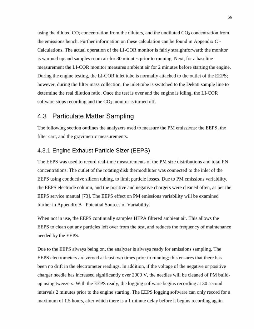
56

using the diluted CO2 concentration from the diluters, and the undiluted CO2 concentration from

the emissions bench. Further information on these calculation can be found in Appendix C -

Calculations. The actual operation of the LI-COR monitor is fairly straightforward: the monitor

is warmed up and samples room air for 30 minutes prior to running. Next, for a baseline

measurement the LI-COR monitor measures ambient air for 2 minutes before starting the engine.

During the engine testing, the LI-COR inlet tube is normally attached to the outlet of the EEPS;

however, during the filter mass collection, the inlet tube is switched to the Dekati sample line to

determine the real dilution ratio. Once the test is over and the engine is idling, the LI-COR

software stops recording and the CO2 monitor is turned off.

4.3 Particulate Matter Sampling

The following section outlines the analyzers used to measure the PM emissions: the EEPS, the

filter cart, and the gravimetric measurements.

4.3.1 Engine Exhaust Particle Sizer (EEPS)

The EEPS was used to record real-time measurements of the PM size distributions and total PN

concentrations. The outlet of the rotating disk thermodiluter was connected to the inlet of the

EEPS using conductive silicon tubing, to limit particle losses. Due to PM emissions variability,

the EEPS electrode column, and the positive and negative chargers were cleaned often, as per the

EEPS service manual [73]. The EEPS effect on PM emissions variability will be examined

further in Appendix B - Potential Sources of Variability.

When not in use, the EEPS continually samples HEPA filtered ambient air. This allows the

EEPS to clean out any particles left over from the test, and reduces the frequency of maintenance

needed by the EEPS.

Due to the EEPS always being on, the analyzer is always ready for emissions sampling. The

EEPS electrometers are zeroed at least two times prior to running; this ensures that there has

been no drift in the electrometer readings. In addition, if the voltage of the negative or positive

charger needle has increased significantly over 2000 V, the needles will be cleaned of PM build-

up using tweezers. With the EEPS ready, the logging software begins recording at 30 second

intervals 2 minutes prior to the engine starting. The EEPS logging software can only record for a

maximum of 1.5 hours, after which there is a 1 minute delay before it begins recording again.

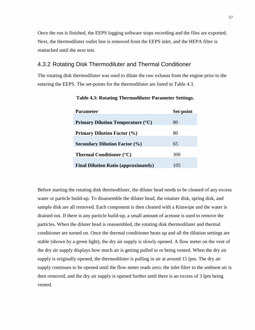
57

Once the run is finished, the EEPS logging software stops recording and the files are exported.

Next, the thermodiluter outlet line is removed from the EEPS inlet, and the HEPA filter is

reattached until the next test.

4.3.2 Rotating Disk Thermodiluter and Thermal Conditioner

The rotating disk thermodiluter was used to dilute the raw exhaust from the engine prior to the

entering the EEPS. The set-points for the thermodiluter are listed in Table 4.3.

Table 4.3: Rotating Thermodiluter Parameter Settings.

Parameter Set-point

Primary Dilution Temperature (°C) 80

Primary Dilution Factor (%) 80

Secondary Dilution Factor (%) 65

Thermal Conditioner (°C) 300

Final Dilution Ratio (approximately) 105

Before starting the rotating disk thermodiluter, the diluter head needs to be cleaned of any excess

water or particle build-up. To disassemble the diluter head, the retainer disk, spring disk, and

sample disk are all removed. Each component is then cleaned with a Kimwipe and the water is

drained out. If there is any particle build-up, a small amount of acetone is used to remove the

particles. When the diluter head is reassembled, the rotating disk thermodiluter and thermal

conditioner are turned on. Once the thermal conditioner heats up and all the dilution settings are

stable (shown by a green light), the dry air supply is slowly opened. A flow meter on the vent of

the dry air supply displays how much air is getting pulled in or being vented. When the dry air

supply is originally opened, the thermodiluter is pulling in air at around 15 lpm. The dry air

supply continues to be opened until the flow meter reads zero; the inlet filter to the ambient air is

then removed, and the dry air supply is opened further until there is an excess of 3 lpm being

vented.

58

The outlet of the thermodiluter is now able to connect to the EEPS and begin sampling. Previous

work found that the rotating disk drifted in temperature due to the hot engine exhaust; therefore,

a small cooling fan was installed to ensure constant thermodiluter temperatures [38].

Once testing is finished, the rotating disk thermodiluter and the thermal conditioner are shut-

down. First, the thermodiluter temperature is reduced from 300 °C to 150 °C to allow the diluter

box to cool down. Once the diluter box has cooled down, the rotating disk thermodiluter is

turned off; the dry air supply is closed; the flow meter is turned off; and the inlet filter is

returned.

4.3.3 Filter Cart

The filter cart was used in this investigation to collect PM mass on the Teflon filters. Based on

previous work, the flow controllers were set to a flowrate of 33 lpm which corresponds to a face

velocity of just under 50 cm/s. Furthermore, the Hot Pocket heater surrounding the cyclone was

set to 55 °C based on previous experimental results [37].

The filter cart flow controllers are left on continuously, this allows them to always be warm. To

calibrate the flow controllers, the sample inlet quick connect fitting is opened, the flow rate is set

to 7 lpm, and the vacuum pumps are turned on. After 5 minutes, the pumps are turned off, the

flow controllers are set to zero, and the quick connect fitting is closed. There are potentiometers

present on the back of the flow controllers; these are used to zero the controllers, which accounts

for any drift in the readings.

Once the flow controllers are calibrated, the Hot Pocket heater is turned on, and the quick

connect fitting is connected to the sampling tube. The flow controllers are both set to 33 lpm, and

prior to the engine start, the filter cart is set to the bypass line.

The first filter collection takes place around 35 minutes into the test. The filter cart is set to

sample 10 minutes before the filters are placed in the filter holders. This enables the filter holders

to heat up to the desired temperature of 30 °C, and avoids any unnecessary cooling of the filters.

Next, the filter cart is set to bypass while the filters are being placed in the holders, and once

ready, the filter cart is set to sample for the desired time (10 – 30 minutes).

59

The filter cart shutdown is straightforward: the Hot Pocket heater is disabled; the flow controllers

are set to zero; and the vacuum pumps are turned off.

4.3.4 Dekati Diluter

The Dekati ejector diluter was used to dilute the exhaust samples before they were collected on

filters. This investigation used identical parameters to those used by Ramos [37]: medium flow

rate, nominal dilution ratio of 9, probe heater temperature of 150 °C, and air heater temperature

of 250 °C.

To start the Dekati diluter, the control software is turned on and begins recording. The sample

flow rate is set to medium so that it can handle the 66 lpm pulled by the vacuum pumps (2 x 33

lpm). The DR is then set by setting solenoids “2” and “3” to open. Following this, the probe and

heater temperatures are set, with the heater temperature requiring a slow ramp up, as the

temperature can overshoot the set-point by a significant amount.

During testing the Dekati diluter is left on. Previous work found that the DR varies significantly

during the test, so it was measured using the CO2 monitor while the filters were sampling [37].

Once the run has finished, the heaters are set to finish, the control software is exited, and the

Dekati diluter is turned off.

4.3.5 Gravimetric Filter Analysis

The gravimetric filter analysis is used for weighing the filters before and after testing. The filter

analysis is done using an on-site Class 100 clean room environment. The original procedure used

by Ramos [37] was based on the US EPA standard procedure for PM gravimetric analysis [74].

The procedure has since been updated based on comments from Sartorius, the scale

manufacturer.

The clean room used in this investigation consists of two rooms separated by sliding doors.

Initially, Class 100 clean room attire are donned in the entry vestibule, and anything being

brought into the clean room is wiped down with wet wipes (moistened with 6% isopropyl/94%

deionized water mix). When entering the clean room, all work surfaces and the forceps are

cleaned with a wet wipe, and an antistatic bracelet is put on. Next, the scale is balanced using

60

two manual leveling feet, and then tared to 0.0000 mg. Following this, the filters that are going

to be balanced are placed on the front of the workbench.

To weigh the filters, they are placed under an electrostatic neutralizer for 10 seconds on each

side, then placed on the scale, and then the chamber door is closed. Once “mg” appears on the

balance, indicating that the measurement is stable, the timer is set for 30 seconds. If “mg”

disappears at any point, the timer is turned off and reset when “mg” reappears. After 30 seconds,

the mass of the filter is recorded. Prior to the filters being weighed, they must be left in the clean

room for at least 24 hours. The 24 hour period is for the filters to reach an equilibrium state at the

clean room’s temperature and humidity. The filters are weighed every 24 hours until consecutive

readings are within 5 µg. The filters must be within the 5 µg prior to testing, and again after

testing.

4.4 Fuel Blending

Figure 4.3: Flow chart showing the fuel blending procedure.

The procedure shown in Figure 4.3 is used to ensure that different fuels can be blended with

repeatability. The first component, i.e., isooctane, is measured to 1 L less than the desired

amount using a volumetric flask, after which it is poured into a jerry can. Next, the remaining

components are measured and poured into the jerry can, after which the remaining 1 L of the

original component is added. The jerry can is then shaken thoroughly to ensure proper mixing.

61

The blend is then used within a day to mitigate the risk of light-end components evaporating.

The flasks are cleaned using acetone between the measurements of different fuels and between

each test.

62

Chapter 5

Experimental Results and Discussion

5.1 Fuel Compositional Effects

The effects of fuel composition on the emissions of particulate matter and gaseous species were

investigated. A previous investigation by Rais [MASc Thesis in Progress] resulted in the

surprising finding that a surrogate gasoline (Fuel 1), consisting of a blend of 65% isooctane

(2,2,4 – trimethylpentane) and 35% toluene by volume, emitted PN concentrations more than an

order of magnitude lower than 91 octane pump gasoline. The difference is illustrated in Figure

5.1, which shows the difference in PN concentration between Fuel 1 and Shell 91 pump gasoline.

Note that the Shell 91 pump gasoline was calculated using the average of 4 tests: two in

December 2016, and two in June 2017. These tests were chosen as they had no measurement

issues, and will be used as a reference case for all blends tested in this study*. Figure 5.1 shows

over an order of magnitude difference in emissions between the two fuels. Evidently, there is a

specific component, or combination of components, in the gasoline that is causing a significant

increase of PM emissions. Rais investigated a number of fuel blends, but was unable to identify

the specific component, or combination of components, responsible for the difference in

emissions [MASc Thesis in Progress].

* These tests were also consistent with Shell 91 pump gasoline tests performed by Rais [MASc Thesis in Progress]

and Ramos [37].

63

Figure 5.1: Comparison of PN concentrations from combustion of Fuel 1 and Shell 91

pump gasoline. Data points represent the average of all tests*. Error bars indicate standard

deviation for the tests averaged.

The fuel test matrix shown in Table 5.1 (repeated from Chapter 4 for reference) was constructed

to further investigate the effects of fuel composition. The focus of this section will be on PN

concentration and PM mass, with additional results examining the recorded PM size distribution

and gaseous emissions. Unless specifically noted, all PM emissions measurements have been

corrected for dilution, and therefore represent engine-out emission levels. In addition, all gaseous

measurements will be specified as wet or dry, depending on the species and the analyzer.

Table 5.2 below shows the number and date of the tests for each fuel. Of note: Fuel 6-2 and 6-3

were removed from the PN concentration results due to the measurements issues outlined in

Section B.1.2 Engine Exhaust Particle Sizer. In addition, testing of Fuel 4 was conducted by Rais

[MASc Thesis in Progress]. Fuels 2, 4, and 6 have only one test, so there are not error bars for

any plots with averaged values. Furthermore, Fuel 3 and Fuel 3R will be combined to produce

three total tests. In terms of PM mass measurements and gaseous emissions, the included tests

will be described in each respective section.

* The number of tests performed can be seen below in Table 5.2

1.00E+04

1.00E+05

1.00E+06

1.00E+07

1.00E+08

0 20 40 60 80 100 120

2-M

inu

te A

vg. P

N C

on

cen

trat

ion

[#/

cm3]

Time [min]

91 pump gasoline Fuel 1

64

It can also be seen that there are significant time gaps between some of the tests, which will be

addressed later on, as measurement issues arose while testing and were corrected prior to the

later tests.

Table 5.1: Fuel composition test matrix by volume percentage.

Isooctane Toluene Pentane Hexane Xylene Naphthalene Solvent #1 Solvent #2 Thiophene

Fuel 1 65.00% 35.00% 0.00% 0.00% 0.00% 0.00% 0.00% 0.00% 0.00%

Fuel 2 62.00% 33.00% 5.00% 0.00% 0.00% 0.00% 0.00% 0.00% 0.00%

Fuel 3 55.00% 30.00% 15.00% 0.00% 0.00% 0.00% 0.00% 0.00% 0.00%

Fuel 4 20.31% 19.34% 0.00% 33.85% 14.51% 0.28% 8.22% 3.39% 0.10%

Fuel 5 20.31% 19.34% 19.34% 14.51% 14.51% 0.28% 8.22% 3.39% 0.10%

Fuel 6 20.37% 19.40% 19.40% 14.55% 14.55% 0.00% 8.24% 3.39% 0.10%

Fuel 7 20.39% 19.42% 19.42% 14.56% 14.56% 0.00% 8.25% 3.40% 0.00%

Fuel 8 22.33% 19.42% 19.42% 14.56% 14.56% 0.00% 9.71% 0.00% 0.00%

Fuel 9 29.13% 22.33% 19.42% 14.56% 14.56% 0.00% 0.00% 0.00% 0.00%

Fuel 10 30.00% 35.00% 20.00% 15.00% 0.00% 0.00% 0.00% 0.00% 0.00%

Fuel 11 52.00% 28.00% 20.00% 0.00% 0.00% 0.00% 0.00% 0.00% 0.00%

Fuel 12 52.00% 28.00% 0.00% 20.00% 0.00% 0.00% 0.00% 0.00% 0.00%

Table 5.2: Test matrix for all fuels by number of tests and the approximate date of the

tests.

# of tests Approx Data

Fuel 1 3 Dec-16

Fuel 1R* 3 Jul-17

Fuel 2 1 Dec-16

Fuel 3 1 Dec-16

Fuel 3R 2 Jul-17

Fuel 4 1 Sep-15

Fuel 5 3 Feb-17

Fuel 6 3 Feb/Mar-17

Fuel 7 2 Jun-17

Fuel 8 2 Jun-17

Fuel 9 2 Jun-17

Fuel 10 2 Jun-17

Fuel 11 3 Jun/Jul-17

Fuel 12 3 Jul-17

* Subscript R indicates a repeat test for a given fuel composition.

65

5.1.1 PN Concentration

Original testing looked at the PN concentration from Shell 91 pump gasoline, compared with the

base blend of 65% isooctane (2,2,4 – trimethylpentane) and 35% toluene.

Fuel blends 2 and 3 were chosen in an attempt to isolate the effect of pentane, as research by

Leach et al. and Warey et al. [36, 19] has shown that pentane plays an important role in the fuel

vaporization. The pentane breaks up the fuel spray earlier, which creates a less homogeneous

mixture prior to combustion [36]. A less homogeneous mixture could lead to increased locally-

rich regions, subsequently leading to high PM emissions. In addition, due to the low boiling

point of pentane, it is possible for there to be surface boiling on the cylinder walls and piston

head [19]. This will increase the PM emissions as it creates a layer of insulation above the piston

head, which reduces evaporation and can lead to increased fuel pooling. This then leads to the

subsequent diffusion burning of the fuel [19]. Fuel 2 had a pentane volume content of 5%, to

reflect the blends investigated by Leach et al. [36], while Fuel 3 increased the pentane content to

15% to more closely reflect the volume content of C5 hydrocarbons present in the analyzed batch

of Shell 91 pump gasoline [61]. Note that Fuel blends 1, 2, and 3 all have the same ratio of

isooctane to toluene (65/35) and differ only in their respective pentane content (0, 5, and 15%

v/v).

Figure 5.2 shows the PN concentrations from the tests performed using these fuels. Clearly, the

PN concentrations for Fuels 1-3 are still significantly lower than gasoline.

66

Figure 5.2: Comparison of PN concentrations from combustion of Fuels 1, 2, 3, and Shell

91 pump gasoline. Data points represent the average of all tests. Error bars indicate

standard deviation for the tests averaged*.

Due to the apparent lack of response to the addition of pentane, a more representative fuel was

tested. The components of Fuel 4, previously tested by Rais [MASc Thesis in Progress], were

chosen to closely resemble the component groups and carbon numbers of the analyzed batch of

Shell 91 pump gasoline. The Fuel 4 blend used hexane to account for both the C5 and C6 ranges,

as light-ends were considered, at the time, to have a minimal effect on PM emissions. As

mentioned earlier, light-ends can be important in fuel blends in order to represent real-world

evaporation behavior [19, 36]. So, Fuel 5 was chosen to investigate whether a combination of

pentane and a different component could be the cause of the PN concentration increase. Fuel 5

has the same components and concentrations as Fuel 4, except that the concentration of hexanes

was reduced from 33.85% to 14.51% with the difference made up by the addition of 19.34%

pentane.

* There are no error bars for Fuel 2 as only one test was performed. Due to the logarithmic scale, the error bars can

be hard to see.

1.00E+04

1.00E+05

1.00E+06

1.00E+07

1.00E+08

0 20 40 60 80 100 1202-M

inu

te A

vg. P

N C

on

cen

trat

ion

[#/

cm3]

Time [min]

91 pump gasoline Fuel 1 Fuel 2 Fuel 3

67

It can be seen in Figure 5.3 that the PN concentration emissions produced by the combustion of

Fuel 5 were similar to those of Shell 91 pump gasoline, indicating that the addition of pentane

was critical. Although Fuel 4 was identical apart from the pentane content replacing some of the

hexane, it produced 95% fewer particles. It should be noted that Fuels 2 and 3 contained pentane

without the same increase in PN concentration, so further tests were conducted to investigate

which component, when combined with pentane, produced the large increase in the PN

concentration.

Figure 5.3: Comparison of PN concentrations from combustion of Fuels 4, 5, and Shell 91


deviation for the tests averaged*.

The average PN concentrations seen in Figure 5.1, Figure 5.2, and Figure 5.3 emphasize the

significant differences between each test; however, the steady-state PN concentration drift during

each test is difficult to evaluate due to the logarithmic scale. Figure 5.4 examines the steady-state

variability of Fuel 5 and the gasoline test. The gasoline test is fairly steady beyond 40 min, but

the Fuel 5 tests exhibited significant increases in the PN concentration with time, although still

small compared to the differences between Fuel 4 and Fuel 5 (Figure 5.3). This is likely due to

* There are no error bars for Fuel 4 as only one test was performed. Due to the logarithmic scale, the error bars can

be hard to see.

1.00E+04

1.00E+05

1.00E+06

1.00E+07

1.00E+08

0 20 40 60 80 100 120

2-M

inu

te A

vg. P

N C

on

cen

trat

ion

[#/

cm3 ]

Time [min]

91 pump gasoline Fuel 4 Fuel 5

68

the increase in background noise in the EEPS particle measurements, and PN concentration

increases, previously found intermittently by both Ramos [37] and Rais [MASc in Progress]

using this engine. Although there is steady-state variability during the tests, there was negligible

test-to-test variability. Furthermore, the differences in the PN concentrations between fuels were

large enough that the variability for a single fuel was not critical. Nevertheless, it is evident that

pentane has a significant effect on the PN concentration and must be investigated further.

Figure 5.4: Comparison of PN concentrations from combustion of Fuel 5 and Shell 91



To isolate the effect of pentane, the components in Fuel 5 were removed one at a time, starting

with the heaviest component, naphthalene, and ending with the lightest component (apart from

pentane), hexane. This was done to identify whether there is a key component that is producing

the high emissions when combusted with pentane. Literature shows there can be a synergistic

effect between individual hydrocarbons producing significantly greater PM emissions than they

would otherwise on their own [75]. Referring back to the test matrix in Table 5.1, it can be seen

that Fuels 6 to 11 each remove one component, with the intent to remove components until there

is a significant decrease in PN concentration. That specific component would then be re-

introduced into the blend to confirm that it is the key component, by an increase in PN

concentration.

0.00E+00

2.00E+06

4.00E+06

6.00E+06

8.00E+06

1.00E+07

1.20E+07

1.40E+07

1.60E+07

1.80E+07

2.00E+07

0 20 40 60 80 100 1202-M

inu

te A

vg. P

N C

on

cen

trat

ion

[#/

cm3 ]

Time [min]

91 pump gasoline Fuel 5

69

Figure 5.5 shows the results of the combustion of Fuels 6 through 11. Interestingly, all of the fuel

blends produced PN concentrations at a relatively similar level to Fuel 5, which was in the same

range as the gasoline tests. Regarding Figure 5.5, it is also evident that removing the heavier

components from each consecutive blend resulted in relatively decreased PN concentrations.

This is reflected by the PN Index which will be discussed in Section 5.1.3.

Figure 5.5: Comparison of PN concentrations from combustion of Fuels 5, 6, 7, 8, 9, 10, and

11. Data points represent the average of all tests. Error bars indicate standard deviation for

the tests averaged.

Due to the long period of time between the original tests (Fuels 1 to 6) and the later tests (Fuels 7

to 11), it was important to ensure that no engine parameters have changed, and that the PN

concentration increases were solely due to changes in fuel composition. Accordingly, the set of

65% isooctane and 35% toluene tests (Fuel 1) were revisited. For clarity, the repeated test set

will be referred to as Fuel 1R. Three tests were done with Fuel 1R to evaluate repeatability. In

Figure 5.6, the averaged results of the three individual Fuel 1 tests can be seen, as well as all

three individual Fuel 1R tests. The PN concentration results from Fuel 1R are visually consistent

with the original results from Fuel 1.

0.00E+00

5.00E+06

1.00E+07

1.50E+07

2.00E+07

2.50E+07

0 20 40 60 80 100 120

2-M

inu

te A

vg. P

N C

on

cen

trat

ion

[#/

cm3]

Time [min]

Fuel 5 Fuel 6 Fuel 7 Fuel 8 Fuel 9 Fuel 10 Fuel 11

70

Figure 5.6: Comparison of PN concentrations from combustion of Fuels 1 and 1R. Error

bars indicate standard deviation for the 2-minute averages.

In Figure 5.6 it can also be seen that Fuel 1R-2 and Fuel 1R-3 produced increased PN

concentrations and had increased variability compared to Fuel 1. This is likely due to issues with

dilution ratio control during tests 2 and 3 of Fuel 1R. The dilution ratio was increasing because of

particle build-up inside the raw gas pump inside the thermodiluter, resulting in higher dilution

ratios, which arose from the reduced raw sample flow. The higher dilution ratios then move the

raw EEPS measurement further towards the analyzers’ detection limits. This will be discussed

further at the end of this section.

With the effect of pentane shown to be repeatable, it is important to determine if there is a

threshold volume content for the PN concentration increase. Since Fuel 11 was essentially a re-

creation of Fuel 3 (20% pentane and 15% pentane, respectively), it is possible that results from

the original test of Fuel 3 were incorrect. Only one test was performed and it showed significant

variability. Repeat tests of Fuel 3 were performed to confirm the results (Fuel 3R-1 and Fuel 3R-

2), and were shown to be repeatable and consistent with the original Fuel 3 tests, indicating that

the pentane content needs to be higher than 15%. The low pentane blends were originally based

on research done by Leach et al. [36], then the ~20% pentane content in Fuels 5 to 11 was

chosen to match the 20% volume content of light-ends in the analyzed gasoline [61]. In Figure

5.7, it can be seen that the tests performed with Fuels 2 (5% pentane), 3 (15% pentane), and 12

1.00E+04

1.10E+05

2.10E+05

3.10E+05

4.10E+05

5.10E+05

0 20 40 60 80 100 120

2-M

inu

te A

vg. P

N C

on

cen

trat

ion

[#/

cm3 ]

Time [min]

Fuel 1-1 Fuel 1-2 Fuel 1-3

0 20 40 60 80 100 120

Time [min]

Fuel 1R-1 Fuel 1R-2 Fuel 1R-3

71

(20% hexane), had significantly lower PN concentrations compared to Fuel 11. As previously

mentioned, Fuels 2 and 3 contain less than 15% pentane, below the threshold value. In addition,

Fuel 12 further isolated the effect of pentane by replacing it with hexane, the next-lightest

component in the larger blends. Clearly, fuels blended with hexane do not provide the same PN

concentration results as pentane, likely due to the lower vapour pressure which will be further

examined in Section 5.1.3. In addition, Figure 5.8 shows the PN concentrations for every test

done. There is a 96% decrease in emissions when going from the high PN fuels (Fuels 5 to 11) to

the low PN fuels (Fuels 1,2,3,4, and 12).

Figure 5.7: Comparison of PN concentrations from combustion of Fuels 2, 3, 11, and 12.

Data points represent the average of all tests. Error bars indicate standard deviation for

the tests averaged.

1.00E+04

1.00E+05

1.00E+06

1.00E+07

0 20 40 60 80 100 120

2-M

inu

te A

vg. P

N C

on

cen

trat

ion

[#/

cm3 ]

Time [min]

Fuel 2 Fuel 3 Fuel 11 Fuel 12

72

Figure 5.8: Comparison of PN concentrations from combustion of the high PN fuels and

low PN fuels. Data points represent the average of all tests. Error bars indicate standard


In Figure 5.7, it is important to note the disparity between the error bars on the low PN fuels and

the high PN fuels. Clearly, the low PN concentration tests have a much higher relative error.

Figure 5.9 displays the average deviation for each test fuel. The values shown were calculated by

taking the average % deviation* of all the 2-minute averages for each test. Following this, the

average % deviation was calculated for each fuel. Evidently, there is a significant increase in the

relative error when testing at low PN concentrations. This is likely because the EEPS is

measuring PN concentrations near its limit of detection. The EEPS limit of detection for particles

below 10nm is 1500 #/cm3 [76]. When sampling at low PN concentrations (raw sample), the

range of EEPS measurements is approximately 1000-4000 #/cm3†, or barely above the detection

limit. This can make measurements difficult, and increases the uncertainty.

* % deviation is calculated by taking the ratio of standard deviation to total PN concentration for each test, then

converting that to a percentage. It makes it easy to compare the variability of tests with vastly different PN

concentrations.

† This range is strongly dependent on the dilution ratio.

1.00E+04

1.00E+05

1.00E+06

1.00E+07

1.00E+08

0 20 40 60 80 100 1202-M

inu

te A

vg. P

N C

on

cen

trat

ion

[#/

cm3]

Time [min]

Fuel 1 Fuel 1R Fuel 2 Fuel 3 Fuel 4 Fuel 5 Fuel 6

Fuel 7 Fuel 8 Fuel 9 Fuel 10 Fuel 11 Fuel 12

pentane

≥19.3%

pentane

≤15%

73

Figure 5.10 illustrates the large gap between the high PN fuels and the low PN fuels. It was

thought that the standard deviation would increase during the tests, similar to the PN

concentration increase. However, that appears to be false as the deviation is fairly constant

throughout each test.

Figure 5.9: Average % deviation for all test fuels. Error bars indicate standard deviation

for the tests averaged.

Figure 5.10: Average % deviation of 2-min averages at 10-min intervals for all test fuels.

0

10

20

30

40

50

60

70

80

Fuel

1

Fuel

1R

Fuel

2

Fuel

3

Fuel

4

Fuel

5

Fuel

6

Fuel

7

Fuel

8

Fuel

9

Fuel

10

Fuel

11

Fuel

12

Ave

rage

% d

evia

tio

n

1

10

100

0 20 40 60 80 100 120

Ave

rage

% D

evia

tio

n

Time [min]



pentane

≤15%

pentane

≥19.3%

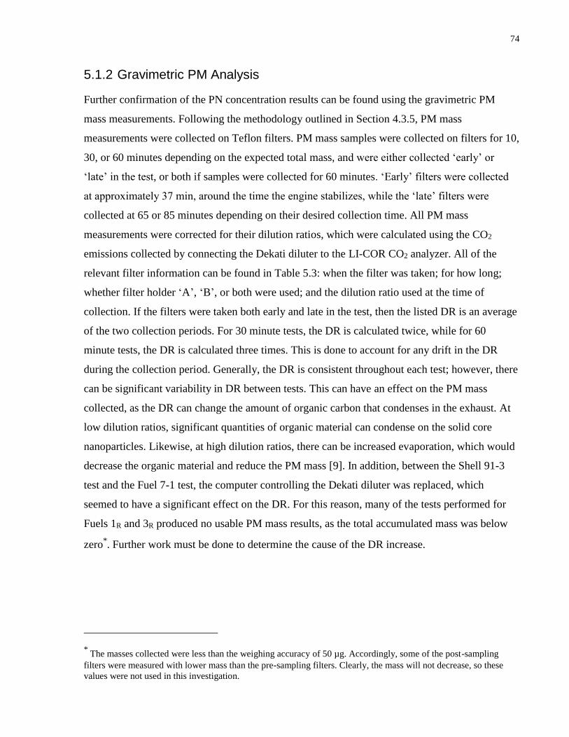
74

5.1.2 Gravimetric PM Analysis

Further confirmation of the PN concentration results can be found using the gravimetric PM

mass measurements. Following the methodology outlined in Section 4.3.5, PM mass

measurements were collected on Teflon filters. PM mass samples were collected on filters for 10,

30, or 60 minutes depending on the expected total mass, and were either collected ‘early’ or

‘late’ in the test, or both if samples were collected for 60 minutes. ‘Early’ filters were collected

at approximately 37 min, around the time the engine stabilizes, while the ‘late’ filters were

collected at 65 or 85 minutes depending on their desired collection time. All PM mass

measurements were corrected for their dilution ratios, which were calculated using the CO2

emissions collected by connecting the Dekati diluter to the LI-COR CO2 analyzer. All of the

relevant filter information can be found in Table 5.3: when the filter was taken; for how long;

whether filter holder ‘A’, ‘B’, or both were used; and the dilution ratio used at the time of

collection. If the filters were taken both early and late in the test, then the listed DR is an average

of the two collection periods. For 30 minute tests, the DR is calculated twice, while for 60

minute tests, the DR is calculated three times. This is done to account for any drift in the DR

during the collection period. Generally, the DR is consistent throughout each test; however, there

can be significant variability in DR between tests. This can have an effect on the PM mass

collected, as the DR can change the amount of organic carbon that condenses in the exhaust. At

low dilution ratios, significant quantities of organic material can condense on the solid core

nanoparticles. Likewise, at high dilution ratios, there can be increased evaporation, which would

decrease the organic material and reduce the PM mass [9]. In addition, between the Shell 91-3

test and the Fuel 7-1 test, the computer controlling the Dekati diluter was replaced, which

seemed to have a significant effect on the DR. For this reason, many of the tests performed for

Fuels 1R and 3R produced no usable PM mass results, as the total accumulated mass was below

zero*. Further work must be done to determine the cause of the DR increase.

* The masses collected were less than the weighing accuracy of 50 µg. Accordingly, some of the post-sampling

filters were measured with lower mass than the pre-sampling filters. Clearly, the mass will not decrease, so these

values were not used in this investigation.

75

Table 5.3: All PM mass measurements with associated filter timing, filter holders, length of

collection, and total average dilution ratio.

Timing Filters Time (min) Dilution Ratio

Fuel 1-1 early A 10 23.3



Fuel 1R-1 late both 10

Fuel 1R-2 late both 30

Fuel 1R-3 late both 60 81.0

Fuel 2 early A 10 25.0


Fuel 3R-1 full both 60 63.2

Fuel 3R-2 full both 60 61.2

Fuel 5-1 early both 10 26.0

Fuel 5-2 both both 10 26.3















Fuel 11-3 late both 10 88.8

Fuel 12-1 full both 60 52.0



76

In Figure 5.11, a strong linear correlation (R2 = 0.9173) can be seen between the PN

concentration and the PM mass for all test fuels with PM mass measurements*. Clearly, as the

PN concentration for a fuel increases, the PM mass increases as well, indicating that the trends

seen for the PN concentrations are also valid for the PM mass measurements. This is evident, as

the high PN fuels follow similar increases, and the low PN fuels have extremely low PM mass

values, similar to their PN concentrations. It is important to note that only the data from the Fuel

1R and Fuel 3R tests is being used (those with reasonable data), and no data from Fuel 2, as the

early tests appeared to be incorrectly heavy in mass. See Appendix B - Potential Sources of

Variability for more information.

These results are reflected by Maricq et al., who found similar decreases in PN concentration and

PM mass with increasing ethanol content [30]. Table 5.4 shows the number of particles per

milligram, which are all within the range of the work of Maricq et al. [30], who found an average

ratio of ~2E+12 particles/mg in soot flames.

* Shell 91 pump gasoline is not included in the trendline. It is included as a reference for the rest of the fuels.

77

Figure 5.11: End average* PN concentration results for each test fuel plotted against the

gravimetric results. Error bars indicate standard deviation for the filters within the

specified tolerance and standard deviation for the tests averaged, for the PM mass and PN

concentration, respectively.

Table 5.4: Calculated† number of particles per mg of PM emissions.

Test Fuel Particles/mg

Fuel 1 1.03E+12

Fuel 3 4.60E+12

Fuel 5 1.83E+12

Fuel 6 2.09E+12

Fuel 7 1.51E+12

Fuel 8 1.41E+12

Fuel 9 1.98E+12

Fuel 10 1.59E+12

Fuel 11 1.70E+12

Fuel 12 2.56E+12

* End average is defined as the last three data points from a test: at 80, 90, and 100 minutes. The tests tend to be

more stable at this point

† These values were calculated simply by dividing the PN concentration by the PM mass for each fuel

Fuel 1

Fuel 3

Fuel 6

Fuel 5

Fuel 7

Fuel 8Fuel 9

Fuel 10

Fuel 11

Fuel 12

Shell 91 pump gasoline

R² = 0.9173

0

5000000

10000000

15000000

20000000

25000000

0 2 4 6 8 10 12 14

Ave

rage

PN

Co

nce

ntr

atio

n [

#/cm

3]

PM mass [mg/m3]

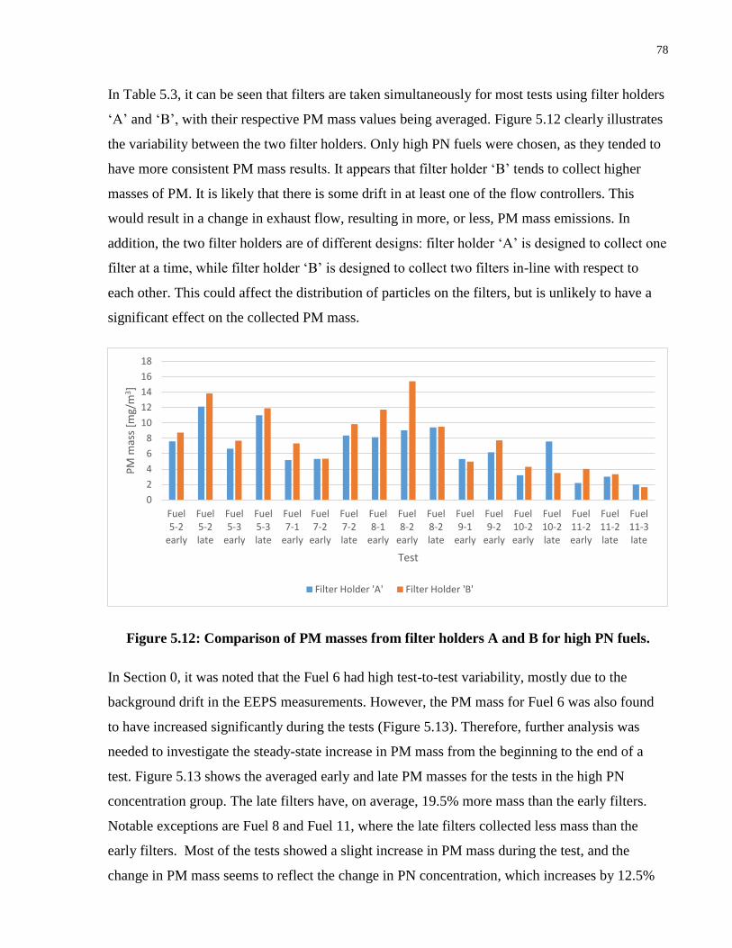
78

In Table 5.3, it can be seen that filters are taken simultaneously for most tests using filter holders

‘A’ and ‘B’, with their respective PM mass values being averaged. Figure 5.12 clearly illustrates

the variability between the two filter holders. Only high PN fuels were chosen, as they tended to

have more consistent PM mass results. It appears that filter holder ‘B’ tends to collect higher

masses of PM. It is likely that there is some drift in at least one of the flow controllers. This

would result in a change in exhaust flow, resulting in more, or less, PM mass emissions. In

addition, the two filter holders are of different designs: filter holder ‘A’ is designed to collect one

filter at a time, while filter holder ‘B’ is designed to collect two filters in-line with respect to

each other. This could affect the distribution of particles on the filters, but is unlikely to have a

significant effect on the collected PM mass.

Figure 5.12: Comparison of PM masses from filter holders A and B for high PN fuels.

In Section 0, it was noted that the Fuel 6 had high test-to-test variability, mostly due to the

background drift in the EEPS measurements. However, the PM mass for Fuel 6 was also found

to have increased significantly during the tests (Figure 5.13). Therefore, further analysis was

needed to investigate the steady-state increase in PM mass from the beginning to the end of a

test. Figure 5.13 shows the averaged early and late PM masses for the tests in the high PN

concentration group. The late filters have, on average, 19.5% more mass than the early filters.

Notable exceptions are Fuel 8 and Fuel 11, where the late filters collected less mass than the

early filters. Most of the tests showed a slight increase in PM mass during the test, and the

change in PM mass seems to reflect the change in PN concentration, which increases by 12.5%

0

2

4

6

8

10

12

14

16

18

Fuel5-2

early

Fuel5-2late

Fuel5-3

early

Fuel5-3late

Fuel7-1

early

Fuel7-2

early

Fuel7-2late

Fuel8-1

early

Fuel8-2

early

Fuel8-2late

Fuel9-1

early

Fuel9-2

early

Fuel10-2early

Fuel10-2late

Fuel11-2early

Fuel11-2late

Fuel11-3late

PM

mas

s [m

g/m

3 ]

Test

Filter Holder 'A' Filter Holder 'B'

79

on average for the high PN tests. The PM mass and PN concentration increase would likely be

closer; however, the PM mass measurements tend to have considerable error, with some

measurements showing significantly different masses between filter holders ‘A’ and ‘B’. Fuels 5,

6, 8, 9, and 11 showed similar PM emissions increases or decreases, while Fuel 10 had a large

variability in the late test between the two filter holders. Using the lower value for Fuel 10 would

lower the PM mass increase to 13.8%, which is significantly closer to the PN concentration

increase.

Figure 5.13: Comparison of PM masses from early and late filter collection. Error bars

indicate standard deviation for the filters within the specified tolerance.

5.1.3 PN Index

The PN Index developed by Leach et al. [33] was used to investigate, and quantify, the impact of

different fuel compositions. The simplified method for calculating the PN Index, based on that

developed by Ramos [37], is shown in Appendix C - Calculations. As mentioned in Section

2.3.2, the double bond equivalent (DBE) value and vapour pressure of each component are

critical for the calculation of the PN Index. The DBE value affects the sooting propensity of a

component, and the dry vapour pressure equivalent (DVPE) determines how quickly the

component evaporates, which can have significant effects on the fuel-air mixing.

0

2

4

6

8

10

12

14

16

18


PM

mas

s [m

g/m

3 ]

Test

Early tests Late tests

80

Table 5.5 shows the calculated PN Index values for all the test fuels, and the associated DBE+1

and DVPE values. All figures shown in this section are based on the values shown in Table 5.5.

It is evident from this table that the inclusion of pentane is essential for realistic PN Index values.

Fuels 1, 2, 3, 4, and 12 do not contain pentane, and all have unfeasibly high PN Index values,

while their PN concentrations and PM mass emissions are all significantly lower than the high

PN fuels.

Table 5.5: DBE, DVPE, and PN Index for all test fuels

Test Fuel DBE+1 DVPE (kpa) PN Index

Fuel 1 2.40 5.40 44.45

Fuel 2 2.32 11.42 20.31

Fuel 3 2.20 23.11 9.52

Fuel 4 2.84 14.15 20.08

Fuel 5 2.84 30.34 9.36

Fuel 6 2.83 30.43 9.29

Fuel 7 2.83 30.48 9.27

Fuel 8 2.75 30.49 9.01

Fuel 9 2.48 30.86 8.02

Fuel 10 2.40 31.81 7.54

Fuel 11 2.12 28.80 7.36

Fuel 12 2.12 11.30 18.76

For the majority of this section, only test fuels that contain pentane content above the threshold

will be examined, as the remaining fuels do not respond as expected. It is important to determine

how accurate the PN Index is, and if it is a reliable predictor for the PN concentration and PM

mass emissions found in this investigation. Figure 5.14 and Figure 5.15 show that the PN Index

correlates well with the PN concentration (R2 = 0.7575) and PM mass (R2 = 0.7643),

respectively.

81

Figure 5.14: End average PN concentration plotted against PN Index values for the high

PN fuels. Error bars indicate standard deviation for the tests averaged.

Figure 5.15: PM mass plotted against PN Index values for the high PN fuels. Error bars


In addition to the PN Index, the PN concentration and PM mass were plotted against the fuels’

DBE+1 values. Results are shown in Figure 5.16 and Figure 5.17. Both figures show good

correlations between the fuels’ DBE+1 values and their respective PN concentration (R2 =

0.7541) and PM mass (R2 = 0.7945). Figure 5.18 shows the strong correlation between the

DBE+1 values and aromatic contents of the fuels. The increase in PM emissions with DBE

values for the fuels is likely due to the sooting propensity of aromatic fuels.

R² = 0.7575

0.00E+00

5.00E+06

1.00E+07

1.50E+07

2.00E+07

2.50E+07

6.00 6.50 7.00 7.50 8.00 8.50 9.00 9.50 10.00End

Avg

. PN

Co

nce

ntr

atio

n [

#/cm

3]

PN Index


R² = 0.7643

0.00E+00

2.00E+00

4.00E+00

6.00E+00

8.00E+00

1.00E+01

1.20E+01

1.40E+01

6.00 6.50 7.00 7.50 8.00 8.50 9.00 9.50 10.00

PM

mas

s [m

g/m

3]

PN Index


82

Figure 5.16: End average PN concentration plotted against DBE+1 values for the high PN

fuels. Error bars indicate standard deviation for the tests averaged.

Figure 5.17: PM mass plotted against DBE+1 values for the high PN fuels. Error bars


R² = 0.7541

0.00E+00

5.00E+06

1.00E+07

1.50E+07

2.00E+07

2.50E+07

1.90 2.10 2.30 2.50 2.70 2.90End

Avg

. PN

Co

nce

ntr

atio

n [

#/cm

3 ]

DBE+1 Values


R² = 0.7945

0.00E+00

2.00E+00

4.00E+00

6.00E+00

8.00E+00

1.00E+01

1.20E+01

1.40E+01

1.90 2.00 2.10 2.20 2.30 2.40 2.50 2.60 2.70 2.80 2.90

PM

mas

s [m

g/m

3 ]

DBE+1 Values


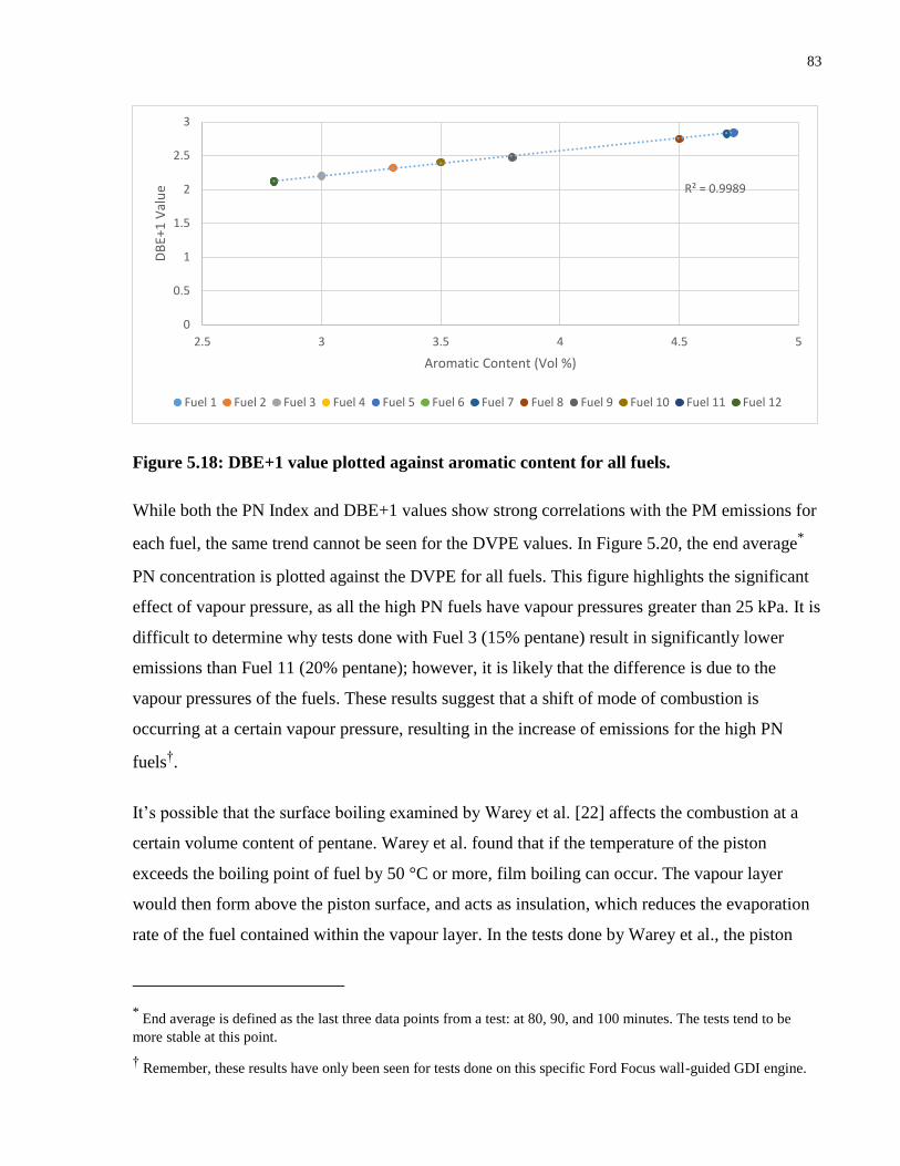
83

Figure 5.18: DBE+1 value plotted against aromatic content for all fuels.

While both the PN Index and DBE+1 values show strong correlations with the PM emissions for

each fuel, the same trend cannot be seen for the DVPE values. In Figure 5.20, the end average*

PN concentration is plotted against the DVPE for all fuels. This figure highlights the significant

effect of vapour pressure, as all the high PN fuels have vapour pressures greater than 25 kPa. It is

difficult to determine why tests done with Fuel 3 (15% pentane) result in significantly lower

emissions than Fuel 11 (20% pentane); however, it is likely that the difference is due to the

vapour pressures of the fuels. These results suggest that a shift of mode of combustion is

occurring at a certain vapour pressure, resulting in the increase of emissions for the high PN

fuels†.

It’s possible that the surface boiling examined by Warey et al. [22] affects the combustion at a

certain volume content of pentane. Warey et al. found that if the temperature of the piston

exceeds the boiling point of fuel by 50 °C or more, film boiling can occur. The vapour layer

would then form above the piston surface, and acts as insulation, which reduces the evaporation

rate of the fuel contained within the vapour layer. In the tests done by Warey et al., the piston

* End average is defined as the last three data points from a test: at 80, 90, and 100 minutes. The tests tend to be

more stable at this point.

† Remember, these results have only been seen for tests done on this specific Ford Focus wall-guided GDI engine.

R² = 0.9989

0

0.5

1

1.5

2

2.5

3

2.5 3 3.5 4 4.5 5

DB

E+1

Val

ue

Aromatic Content (Vol %)

Fuel 1 Fuel 2 Fuel 3 Fuel 4 Fuel 5 Fuel 6 Fuel 7 Fuel 8 Fuel 9 Fuel 10 Fuel 11 Fuel 12

84

temperature was estimated at 120 °C, which is 84 °C and 52 °C higher than the boiling point of

pentane and hexane, respectively [19]. This is a small difference between pentane and hexane,

making it unlikely that surface boiling is the cause of the PM emissions discrepancy. In addition,

Fatouraie et al. determined the importance of the piston temperature, and how it affects the fuels

ability to evaporate from the surface of the piston head. Low piston temperatures can also lead to

significant soot production, as there will be low fuel vaporization off the piston head [20].

Further information regarding piston head temperature is required to determine if surface boiling

is present in these experiments.

A more likely possibility comes from the research done by Leach et al. [36], who found that PN

emissions decreased with decreasing vapour pressure, if there was no pentane present in the fuel.

They found that pentane was causing the spray to break up earlier, and making the fuel spray less

homogeneous, and leading to a significant increase in PN concentration (a little under an order of

magnitude). It’s possible that an extreme version of this trend is occurring, and that below a

certain vapour pressure the fuel is not evaporating similarly to real-world conditions. This is

likely due to differences in engine design, as the engine used by Leach et al. [36] was spray-

guided, and the engine used in this investigation is wall-guided. Fatouraie et al. [20] used an

engine similar to the one used in this investigation, and found interesting results regarding fuel

rebound. Fuel rebound is a phenomenon where the fuel rebounds off the piston, reducing the fuel

impingement (Figure 5.19). Higher fuel rebound leads to lower soot formation, as there is less

fuel film on the piston head, leading to reduced diffusion burning [20]. It is possible that the

pentane is breaking up the spray earlier [36], causing the spray to lose momentum, which would

result in a lower amount of fuel rebound [20]. Following this, it is possible that the fuels without

pentane maintain their momentum and rebound off the piston head, reducing the fuel film and

leading to a more homogeneous combustion. It is important to note that fuel boiling can also lead

to increased fuel rebound, which then suppresses soot formation [20]. This contradicts the fuel

boiling effect seen by Warey et al. [19]; however, it is possible that the differences are due to

engine design.

85

Figure 5.19: Fuel spray images with coolant temperatures of 25 °C (a) and 90 °C (b) [20].

Furthermore, Catapano et al. [77] found that the presence of ethanol enhanced the evaporation of

all the light-end components, leaving the mid- to heavy-components as a fuel film on the piston

head. Not only does ethanol isolate the components with higher sooting tendencies, it also

increased fuel impingement on the piston head due to the volatility properties of the

ethanol/gasoline blend [77]. While it is important to recognize the distinctions between ethanol

and pentane, it is possible that the pentane is playing a similar role in the fuel blends used in this

investigation. Pentane would then evaporate quickly, increase fuel impingement on the piston

head, and leave the heavier components to form the fuel film. Diffusion burning of this film can

then lead to significant increases in PM emissions.

As there is a 96% decrease in PN concentration between the high PN group and the low PN

group, it is likely that there is a different mode of soot production in the high PN fuels compared

to that in the low PN fuels. It is hypothesized that in the low PN fuels there may be little to no

diffusion burning on the piston, and the soot particles are only being produced from locally-rich

regions. It is also possible that the combustion is similar to a pre-mixed engine, and whatever

86

mechanism is occurring is leading to a significant increase in mixing, with little locally-rich

regions. These hypothesis will be examined further in the rest of this chapter.

Figure 5.20: End average PN concentrations plotted against DVPE for all fuels. Error bars

indicate standard deviation for the tests averaged.

5.1.4 PN Size Distribution

The PN size distribution was averaged for all tests with each fuel*, by taking an arithmetic

average of the mobility diameter distribution produced by the EEPS instrument from a time

interval spanning from 30 minutes to 100 minutes in each test. As previously discussed in

Section 1.3.2, smaller particles have greater health implications, as they can more easily enter the

lungs and translocate from the lungs into circulation, potentially leading to cardiovascular

diseases.

Figure 5.21 and Figure 5.22 show the normalized PN size distribution for the low and high PN

groups respectively. Even within each group, the differences in PN concentration were making it

difficult to accurately assess and compare the PN size distributions between each fuel. It was

important to normalize the PN size distributions for each fuel by calculating the percentage of

the total concentration at each particle size. The PN size distribution for the higher group appears

* The EEPS records mobility equivalent diameters, as not all particles are spherical.

0.00E+00

5.00E+06

1.00E+07

1.50E+07

2.00E+07

2.50E+07

0.00 5.00 10.00 15.00 20.00 25.00 30.00 35.00

End

Avg

. PN

Co

nce

ntr

atio

ns

[#/c

m3 ]

DVPE [kpa]


High PN fuels

87

to be slightly more consistent, likely due to the higher number of particles reducing measurement

error.

Figure 5.21: PN size distribution for all the low PN fuels. Error bars indicate standard


Figure 5.22: PN size distribution for all the high PN fuels. Error bars indicate standard


In Figure 5.23, the normalized PN size distributions for all fuels can be seen. Since there were

numerous fuels tested, Figure 5.24 averaged the high and low PN concentrations for a more

0

2

4

6

8

10

12

14

1 10 100 1000No

rmal

ized

Par

ticl

e C

on

cen

trat

ion

[%

}

Particle Size [nm]

Fuel 1 Fuel 2 Fuel 3 Fuel 4 Fuel 12

0

2

4

6

8

10

12

14

16

1 10 100 1000No

rmal

ized

Par

ticl

e C

on

cen

trat

ion

[%

}

Particle Size [nm]


88

direct comparison of the two groups. Similar to the results found by Ramos and Mireault [37,

38], the high PN group produced particles with a peak size at approximately 70-80nm; however,

the low PN group produced increased relative numbers smaller particles*, with a peak size at

approximately 50-60nm. It is important that the difference in concentration between the particles

created by the fuels be taken into account. It is likely that the second peak, associated with

nucleation mode particles (near 10 nm), seen in the low PN group, is due to the low PN

concentrations. According to Wang et al., lower PN concentrations reduce the available soot

surface area for HC condensation; thus, HC nucleation is more likely to occur [22]. Therefore,

for the low PN group, decreases in the accumulation mode particles leads to an increase in

nucleation mode particles. Again, note that while the relative number of nucleation mode

particles is greater in the low PN group, due to the order of magnitude lower overall number of

particles, the actual number of nucleation mode particles in the low PN group is less than in the

high PN group (Figure 5.25).

* Note that the PN quantities are normalized.

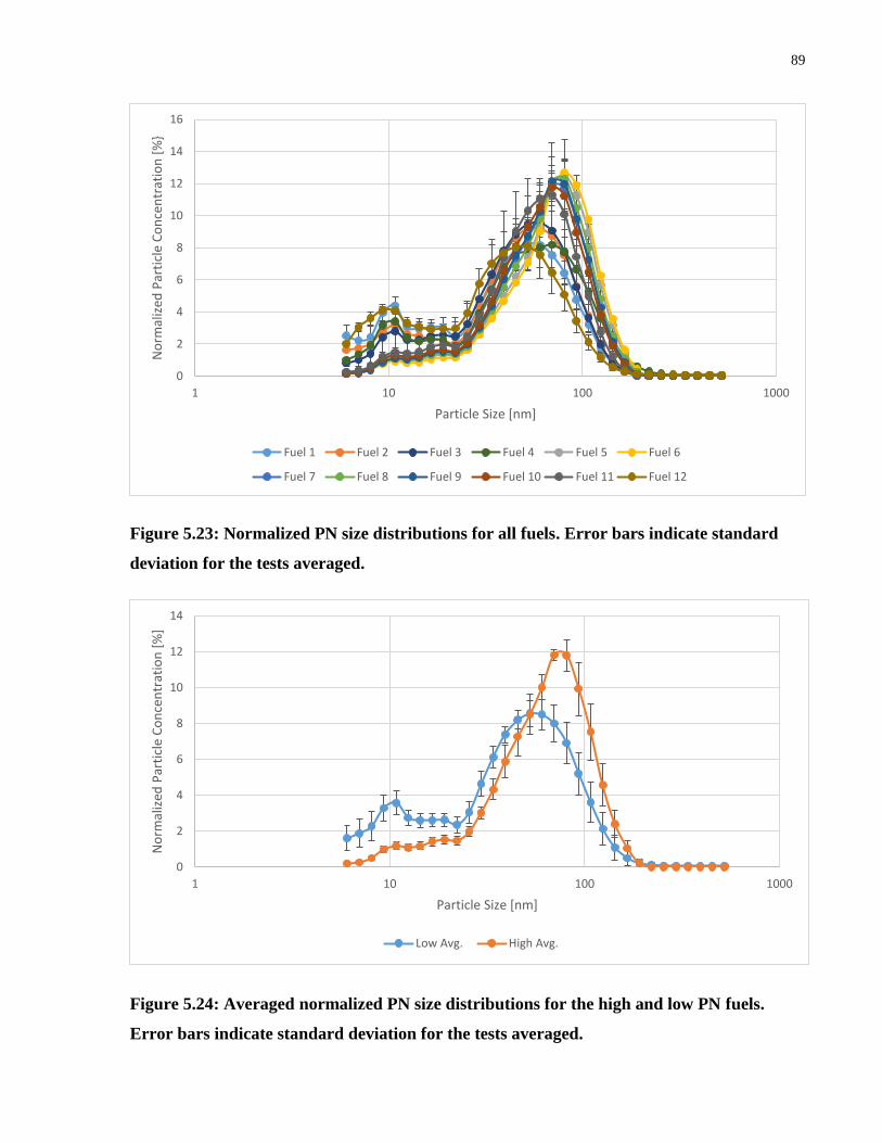
89

Figure 5.23: Normalized PN size distributions for all fuels. Error bars indicate standard


Figure 5.24: Averaged normalized PN size distributions for the high and low PN fuels.

Error bars indicate standard deviation for the tests averaged.

0

2

4

6

8

10

12

14

16

1 10 100 1000

No

rmal

ized

Par

ticl

e C

on

cen

trat

ion

[%

}

Particle Size [nm]



0

2

4

6

8

10

12

14

1 10 100 1000

No

rmal

ized

Par

ticl

e C

on

cen

trat

ion

[%

]

Particle Size [nm]

Low Avg. High Avg.

90

Figure 5.25: Corrected PN size distributions for all fuels.

An important comparison can be made between the corrected size distributions for the low and

high PN fuels. Catapano et al. [78] tested an engine in both a PFI and GDI engine configuration,

and recorded the PN size distributions*. Figure 5.26 demonstrates the remarkable similarity

between the size distributions for the PFI engine setup to the size distributions for the low PN

fuels, particularly Fuels 1, 2, and 12, that have the lowest concentrations†. When compared to the

high PN fuels and the GDI setup (Figure 5.27), it can be seen that the low PN fuels and PFI

configuration have a secondary peak around 10 nm, and both tests have PN concentrations

approximately an order of magnitude lower than their counterparts, the high PN fuels and the

GDI configuration, respectively. Additionally, the GDI size distribution also looks remarkably

similar to the high PN fuels. Both size distributions are dominated by larger diameter particles.

The similarities between the low PN fuels and the PFI configuration further enforce the idea that

* Their values were also recorded using an EEPS.

† Again, remember that it is difficult to accurately compare total PN concentrations as there are many contributing

factors. The engines are being run at different loads, and potentially at different dilution ratios.

0.00E+00

5.00E+06

1.00E+07

1.50E+07

2.00E+07

2.50E+07

3.00E+07

3.50E+07

4.00E+07

1 10 100 1000

dN

/dlo

gDp

[#/c

m3 ]

Particle Size [nm]



91

the low PN fuels are experiencing a different mode of combustion. From these results, it appears

as though the low PN fuels may be operating with almost pre-mixed combustion.

Figure 5.26: Comparison of the corrected PN size distribution for the low PN fuels (left)

and the PFI configuration tested by Catapano et al. (right) [78].

Figure 5.27: Comparison of the corrected PN size distribution for the high PN fuels (left)

and the GDI configuration tested by Catapano et al. (right) [78].

0.00E+00

2.00E+05

4.00E+05

6.00E+05

8.00E+05

1.00E+06

1.20E+06

1 10 100 1000

dN

/dlo

gDp

[#/c

m3 ]

Particle Size [nm]

Fuel 1

Fuel 2

Fuel 3

Fuel 4

Fuel 12

0.00E+00

5.00E+06

1.00E+07

1.50E+07

2.00E+07

2.50E+07

3.00E+07

3.50E+07

4.00E+07

1 10 100 1000

dN

/dlo

gDp

[#/c

m3]

Particle Size [nm]

Fuel 5

Fuel 6

Fuel 7

Fuel 8

Fuel 9

Fuel 10

Fuel 11

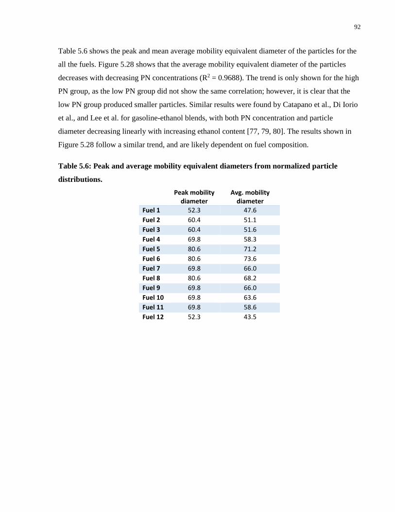
92

Table 5.6 shows the peak and mean average mobility equivalent diameter of the particles for the

all the fuels. Figure 5.28 shows that the average mobility equivalent diameter of the particles

decreases with decreasing PN concentrations (R2 = 0.9688). The trend is only shown for the high

PN group, as the low PN group did not show the same correlation; however, it is clear that the

low PN group produced smaller particles. Similar results were found by Catapano et al., Di Iorio

et al., and Lee et al. for gasoline-ethanol blends, with both PN concentration and particle

diameter decreasing linearly with increasing ethanol content [77, 79, 80]. The results shown in

Figure 5.28 follow a similar trend, and are likely dependent on fuel composition.

Table 5.6: Peak and average mobility equivalent diameters from normalized particle

distributions.

Peak mobility diameter

Avg. mobility diameter

Fuel 1 52.3 47.6

Fuel 2 60.4 51.1

Fuel 3 60.4 51.6

Fuel 4 69.8 58.3

Fuel 5 80.6 71.2

Fuel 6 80.6 73.6

Fuel 7 69.8 66.0

Fuel 8 80.6 68.2

Fuel 9 69.8 66.0

Fuel 10 69.8 63.6

Fuel 11 69.8 58.6

Fuel 12 52.3 43.5

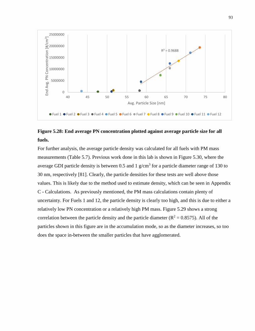
93

Figure 5.28: End average PN concentration plotted against average particle size for all

fuels.

For further analysis, the average particle density was calculated for all fuels with PM mass

measurements (Table 5.7). Previous work done in this lab is shown in Figure 5.30, where the

average GDI particle density is between 0.5 and 1 g/cm3 for a particle diameter range of 130 to

30 nm, respectively [81]. Clearly, the particle densities for these tests are well above those

values. This is likely due to the method used to estimate density, which can be seen in Appendix

C - Calculations. As previously mentioned, the PM mass calculations contain plenty of

uncertainty. For Fuels 1 and 12, the particle density is clearly too high, and this is due to either a

relatively low PN concentration or a relatively high PM mass. Figure 5.29 shows a strong

correlation between the particle density and the particle diameter (R2 = 0.8575). All of the

particles shown in this figure are in the accumulation mode, so as the diameter increases, so too

does the space in-between the smaller particles that have agglomerated.

R² = 0.9688

0

5000000

10000000

15000000

20000000

25000000

40 45 50 55 60 65 70 75 80

End

Avg

. PN

Co

nce

ntr

atio

n [

#/cm

3 ]

Avg. Particle Size [nm]


94

Table 5.7: Average effective particle densities for all fuels

density (g/cm3)

Fuel 1 17.2

Fuel 3 3.0

Fuel 5 2.9

Fuel 6 2.3

Fuel 7 4.4

Fuel 8 4.3

Fuel 9 3.4

Fuel 10 4.7

Fuel 11 5.6

Fuel 12 9.1

Figure 5.29: Average effective particle density plotted against average mobility equivalent

diameter for the high PN fuels

R² = 0.8575

0.0

1.0

2.0

3.0

4.0

5.0

6.0

7.0

50 55 60 65 70 75

Ave

rage

Eff

ecti

ve P

arti

cle

Den

sity

[g

/cm

3]

Average Mobility Equivalent Diameter [nm]

95

Figure 5.30: Effective density plotted against mobility diameter from previous research

performed with this engine [81]

5.1.5 Gaseous Emissions

The emissions bench and FTIR were used to measure and record both regulated and un-regulated

gaseous emissions. The emissions bench recorded only regulated emissions, while the FTIR

provided hydrocarbon speciation and recorded some regulated compounds. However, the FTIR

is unable to measure homonuclear molecules; thus, the O2 emissions were only recorded using

the emissions bench. This section will examine and compare the gaseous species for each test

fuel, and the following section (Section 5.1.6) will examine any trends between the PM

emissions and the gaseous species.

96

Regulated Emissions

Figure 5.31 and Figure 5.32 display the regulated gaseous emissions measured with the FTIR

and the emissions bench, respectively. The FTIR measures all species wet, and the emissions

bench measures THC and NOx wet, and CO2 and O2 dry. The recorded emissions are generally

typical of a GDI engine running at slightly rich conditions [53]. There were issues with the

recorded CO values for Fuels 1, 2, 5, and 6: the FTIR values were higher than normal, and the

emissions bench values were clearly incorrect. All of these fuels were tested during the early

testing period, prior to the engine’s O2 sensor replacement. As mentioned in Appendix B -

Potential Sources of Variability, the drift in the old O2 sensor resulted in a richer fuel-air mixture,

which is likely the reason for increased recorded CO values from the FTIR. The NDIR CO

analyzer on the emissions bench was likely poorly calibrated, as the values are impossibly high.

The exaggerated values are most apparent when examining Fuel 1 and Fuel 1R, and thus, only the

later tests for Fuel 3 (Fuel 3R-1 and Fuel 3R-2) were used for this section.

Fuel effects on the gaseous emissions appear to be limited. Measured CO and THC values appear

to increase with the heavier fuel blends (Fuels 5-11). The measured O2 values have a significant

increase during the latter tests (Fuel 7 onwards), likely due to the earlier tests running at richer

air-fuel mixtures.

Comparing the data in Figure 5.31 and Figure 5.32, it can be seen that there are disparities

between the measurements recorded by the FTIR and by the emissions bench. These differences

were discussed thoroughly by Ramos. He discovered that the CO2 and CO values measured by

the FTIR were consistently lower by approximately 7% and 2%, respectively, while the NOx

values measured by the FTIR were approximately 5% higher [37]. In this experiment, some of

these measurement differences appear to be exacerbated, as the FTIR measurements of CO2 and

CO were lower than the emissions bench by ~15% and 17%, respectively. However, the NOx

measured by the FTIR was only a ~1% increase compared to the NOx measured by the emissions

bench. Finally, the H2O content calculated by the FTIR was ~13% lower than the H2O content

calculated by the emissions bench, which would directly affect the dry calculations for each

analyzer, with a relative increase for the emissions bench. While the raw values show some

differences; in general, the two analyzers show similar results for all the gaseous emissions.

97

Figure 5.31: Regulated emissions measured by the FTIR for all test fuels. Error bars

indicate standard deviation for the tests averaged.

Figure 5.32: Regulated emissions measured by the emissions bench for all test fuels*. Error

bars indicate standard deviation for the tests averaged.

* Fuel 9 and the first test of Fuel 10 were removed due to measurement issues with the emissions bench.

0

2

4

6

8

10

12

14

H₂O [%] CO₂ Dry [%] CO Dry [10³ ppm] NOx Wet [10³ ppm]

Co

nce

ntr

atio

n [

% o

r 1

03

pp

m]

Fuel 1

Fuel 1R

Fuel 2

Fuel 3

Fuel 4

Fuel 5

Fuel 6

Fuel 7

Fuel 8

Fuel 9

Fuel 10

Fuel 11

0

2

4

6

8

10

12

14

CO₂ Dry [%] Calc. H₂O [%] O₂ Dry [%] THC [10³ ppm] -C₃ basis

NOₓ [10³ ppm] CO Dry [10³ppm]

Co

nce

ntr

atio

n [

% o

r 1

03

pp

m]

Fuel 1

Fuel 1R

Fuel 2

Fuel 3

Fuel 4

Fuel 5

Fuel 6

Fuel 7

Fuel 8

Fuel 9

Fuel 10

Fuel 11

Fuel 12

98

FTIR Speciation

In addition to the regulated exhaust emissions, the FTIR also provides a hydrocarbon speciation

of the exhaust. Figure 5.33 and Figure 5.34 display the measurements from the FTIR for all

fuels. The FTIR speciation is important, as certain exhaust constituents can be used as predictors

of PM emissions, or as indicators of fuel composition. All values are similar to previous values

seen by Ramos [37], with certain exaggerated values seen for Fuels 1-4, potentially due to the

significant changes in fuel composition or the richer fuel-air mixtures. In the following section,

the PM emissions for each test fuel will be compared to the gaseous constituents to identify any

trends.

Figure 5.33: Hydrocarbon emissions measured by the FTIR for all test fuels (wet). Error


0

20

40

60

80

100

120

140

160

Methane Ethylene Acetylene Isobutylene Formaldehyde Acetaldehyde

Co

nce

ntr

atio

n [

pp

m]

Fuel 1

Fuel 1R

Fuel 2

Fuel 3

Fuel 4

Fuel 5

Fuel 6

Fuel 7

Fuel 8

Fuel 9

Fuel 10

Fuel 11

Fuel 12

99

Figure 5.34: Hydrocarbon emissions measured by the FTIR for all test fuels (wet). Error


5.1.6 PM emissions vs. Gaseous Species

During previous work, Ramos found that certain constituents in the exhaust can be used as

markers, or predictors, of PM emissions. In this section, the focus will be on PN concentrations,

as Sections 5.1.2 and 5.1.3 previously demonstrated a correlation between PM mass and PN

concentrations. For a larger sample size, each individual test, not fuel averages, will be

considered*. Outliers were excluded when calculating trendlines. The gaseous constituents that

were found to have strong correlations with the PM emissions were: THC, pentane, and 1, 3

butadiene.

First, in Figure 5.35 it is important to note that the PN concentrations are well correlated with the

emissions bench THC values (R2 = 0.9299), indicating that high THC emissions are a good

predictor of PN concentration emissions. Warey et al. [19] found similar results comparing PM

mass emissions to THC emissions. They discovered that the THC emissions followed similar

trends to the PM mass emissions under identical conditions [19]. This is likely due to an increase

in locally rich regions forming due to poor mixing, and fuel impingement on the piston head and

* The tests of Fuel 6-2 and 6-3 were excluded due to their inflated PN concentration values.

0

20

40

60

80

100

120

140

160

180

Propylene 1,3 butadiene Toluene Pentane Benzene Ethane

Co

nce

ntr

atio

n [

pp

m]

Fuel 1

Fuel 1R

Fuel 2

Fuel 3

Fuel 4

Fuel 5

Fuel 6

Fuel 7

Fuel 8

Fuel 9

Fuel 10

Fuel 11

Fuel 12

100

cylinder walls. This correlation indicates that the hydrocarbons are forming in the same process

as the PM emissions.

Following this, Figure 5.36 shows that the exhaust pentane concentrations are well correlated

with PN concentrations (R2 = 0.9141). Figure 5.37 attempts to explain this correlation, as the

pentane content in the exhaust is very well correlated with the THC values from the emissions

bench (R2 = 0.8716). It is possible that some of the pentane in the exhaust results from UBHC

(the unburned fuel would contain pentane for some fuel blends), in addition to the pentane being

produced during the combustion process. However, no trends were found when comparing

pentane content in the fuel to pentane concentration in the exhaust.

Unfortunately, Fuels 1-1, 1-2, 1-3, 2, and 3-1 did not show the same trends, and they all have

elevated THC values compared to their PN concentrations. Examining Figure 5.37, it is clear that

both the emissions bench and FTIR record high THC and pentane emissions. This indicates that

there is an engine issue, and not a measurement issue, as it is unlikely both analyzers would be

incorrect. This is likely due to the tests running slightly richer, as they were all tested prior to the

O2 sensor replacement.

All of the tests performed prior to the O2 sensor replacement have been circled on Figure 5.35

and Figure 5.36. Clearly, the circled low PN fuels are not behaving similarly to the rest of the

tests. While all the other tests show an increase in PN concentration with an increase in THC, the

circled low PN tests have a significant increase in THC and pentane emissions, without the

correlated increase in PN concentration. This indicates that there is a shift in the mode of

combustion, potentially pre-mixed for the low PN fuels, similar to what is mentioned in Section

5.1.3. Soot is formed at significantly rich conditions (phi greater than 2); thus, under the

assumption that the low PN fuels are behaving similarly to pre-mixed combustion, it is expected

that enrichening the fuel-air mixture will not result in an increase in emissions. Generally, GDI

engines have locally-rich regions that will produce significant amounts of soot, but in the pre-

mixed mode, these regions will not exist. This may explain why the high PN fuels saw an

associated increase in the PN concentration, while the low PN fuels did not.

101

Figure 5.35: End average PN concentration for all fuels plotted against emissions bench

THC concentration. Error bars indicate standard deviation for the sampling period.

Figure 5.36: End average PN concentration for all fuels plotted against FTIR pentane

concentration. Error bars indicate standard deviation for the sampling period.

R² = 0.9299

0.00E+00

5.00E+06

1.00E+07

1.50E+07

2.00E+07

2.50E+07

600 700 800 900 1000 1100 1200 1300 1400End

Avg

. PN

Co

nce

ntr

atio

n [

#/cm

3]

Emissions Bench THC [ppm]



R² = 0.9141

0.00E+00

5.00E+06

1.00E+07

1.50E+07

2.00E+07

2.50E+07

60 70 80 90 100 110 120

End

Avg

. PN

Co

nce

ntr

atio

n [

#/cm

3 ]

FTIR Pentane [ppm]



102

Figure 5.37: FTIR pentane concentration plotted against emissions bench THC

concentration for all fuels. Error bars indicate standard deviation for the sampling period.

Furthermore, Figure 5.38 shows a strong correlation between the PN concentrations and 1,3

butadiene concentration in the exhaust (R2 = 0.8481). From the gasoline analysis, there is

0.002% 1,3 butadiene by volume in Shell 91 pump gasoline and 0% in the test blends [61],

indicating that the 1,3 butadiene found in the exhaust is a result of combustion. Figure 5.39

shows that 1,3 butadiene has a strong correlation with the fuels DBE+1 value (R2 = 0.7611). 1,3

butadiene has two double bonds, and may be a marker for the DBE values for the fuels.

However, it is important to note the small range and concentrations of the 1,3 butadiene values.

There is very little difference in concentration between the high PN and low PN fuels.

R² = 0.8716

0

20

40

60

80

100

120

140

600 700 800 900 1000 1100 1200 1300 1400 1500

FTIR

Pen

tan

e [p

pm

]

Emissions Bench THC [ppm C3]



103

Figure 5.38: End average PN concentrations for high PN fuels plotted against FTIR 1,3

butadiene concentration. Error bars indicate standard deviation for the tests averaged.

Figure 5.39: FTIR 1,3 butadiene concentration plotted against DBE+1 values for high PN

fuels.

R² = 0.8481

0.00E+00

5.00E+06

1.00E+07

1.50E+07

2.00E+07

2.50E+07

4 5 6 7 8 9 10 11 12

End

Avg

. PN

Co

nen

ctra

tio

n [

#/cm

3]

1,3 butadiene [ppm]


R² = 0.7611

0

2

4

6

8

10

12

2.00 2.10 2.20 2.30 2.40 2.50 2.60 2.70 2.80 2.90 3.00

1,3

bu

tad

ien

e [p

pm

]

DBE+1Fuel 1 Fuel 1R Fuel 2 Fuel 3 Fuel 4 Fuel 5 Fuel 6


104

Chapter 6

Conclusions and Recommendations

The main goal of this thesis was to solve the issue previously identified by Rais [MASc Thesis in

Progress]: the cause of the large PM emissions gap between the 65% isooctane and 35% toluene

fuel blend and the Shell 91 pump gasoline. Rais found that introducing gasoline additives, heavy

hydrocarbons, and oil did not produce any significant increase of PM emissions. Previous tests

done by Rais and the literature were used to identify components that may be the source of this

increase [MASc Thesis in Progress]. The additional components identified were the basis for the

tests performed in this work. The results of these tests generated the following conclusions and

recommendations.

6.1 Conclusions

The primary takeaway of this work is the significant role that light-end components can have on

the PM emissions from a GDI engine. In this investigation, pentane was used to mimic the light-

end components found in Shell 91 pump gasoline, approximately 20% [61]. At pentane content

15% or lower, it was found that the end average PN concentration emissions were 96% lower

than those with pentane content of 19.3% or higher. This is likely due to a shift in the mode of

combustion due to the changes in vapour pressure. Currently, the best hypothesis is that the low

PN fuels are behaving similarly to a pre-mixed mode of combustion. This could be due to the

lack of spray break up from the light-end components, and the associated increase in fuel

rebound.

The PM mass results were shown to be highly correlated with the PN concentration results, with

a coefficient of determination, or R2 value, of 0.8942. This implies that it is possible to use the

PN concentration results to analyze overall trends of the PM emissions. There was significant

error in the filter measurements due to the discrepancy in gravimetric masses between filter

holder ‘A’ and filter holder ‘B’, as well as between the ‘early’ and ‘late’ filters. This should be

investigated further in the future.

Normalized PN distribution results showed a skew towards larger particles for the high PN

concentration fuels, which had a peak mobility diameter at ~70-80 nm, while the low PN group

105

had a peak mobility diameter at ~50-60 nm. Within each PN concentration group there were

slight changes to particle distribution based on fuel composition; however, those results were

considered insignificant in comparison to the discrepancy between the high and low PN fuels.

The comparison of the size distribution for the low PN fuels and the PFI configuration further

supports the hypothesis that the low PN fuels are behaving similarly to a pre-mixed engine.

The simplified PN Index used in this investigation proved to be effective as a predictor for both

PN concentration and PM mass of the high PN fuels, with R2 values of 0.7575 and 0.7643,

respectively. The low PN fuels, apart from Fuel 3, showed little correlation with the PN Index,

and had unrealistic PN Index values. Furthermore, the DBE+1 values for the high PN fuels also

showed a great correlation, which makes sense as it reflects the aromatic content of the fuel

blend. While there was not a significant correlation between vapour pressure and PN

concentration for the high PN fuels, it was found that the vapour pressure could potentially

determine whether a fuel blend will produce high or low PM emissions. Fuel 3, which had 15%

pentane content and a vapour pressure of 23 kPa, had a PN concentration an order of magnitude

lower than Fuel 11, which had 20% pentane content and a vapour pressure of 29 kPa.

The gaseous emissions found in this investigation were generally similar to those found in GDI

engines running at slightly rich conditions. It was found that several of the exhaust constituents

correlated well with the PN concentrations. These findings have the potential to be used as

predictors for PM emissions with different fuel blends, and can potentially provide insight into

the production of particles inside the engine. Both THC and pentane emissions showed a good

correlation with PM emissions, indicating that they are being produced during the same process.

1,3 butadiene also shows a strong correlation with both PM emissions, likely due to an increase

in the DBE values, or aromatic content, of the fuel blends. Once again, the low PN fuels lack of

response to richer combustion indicates that the combustion was likely more pre-mixed, and thus

did not experience an increase in soot production.

6.2 Recommendations

There are many improvements that can be made for future work on this engine. Proposed

changes in the procedure and apparatus for this instrument are listed below.

106

The filters should be taken at a lower dilution ratio, and measurements should be more

consistent, with filters being taken at the same time every test. This time should be past

40 minutes, as that is the time it takes the PN concentrations to stabilize. In addition, the

time should be determined based on when the engine was switched to the highway

condition.

Introduce DAQ measurements for injection timing and duration, and valve timing.

All recording times should be synchronized, or all analyzers should provide data to the

same computer, to allow for easier comparisons between instruments.

If using the two solvents (APSOL #1 and #2), gas chromatography should be used to

provide a compositional report. Knowing exactly which hydrocarbons are present will

allow for a more accurate gasoline substitute, and will provide more information

regarding the PN Index calculation.

EC/OC data would be very helpful in determining the content of the PM emissions being

measured. For PN concentration, this could also be done by introducing a

Thermodenuder into the EEPS sample line to remove the organic species. Testing the

same fuel with and without the Thermodenuder would provide the number of elemental

carbon particles and the number of organic carbon particles.

Ion analysis can be performed to look for metals in the filters. Due to the drastic decrease

in emissions, it is possible that the PM emissions from the low PN group are solely from

the lube oil. Tracing the metals in the filters can provide some insight into the presence of

metals.

In terms of calculating particle density, it may be important to use an aerosol particle

mass analyzer to provide accurate measurements. Particle density can provide further

information regarding the characteristics of the particles emitted, and can be used to

double check the PN concentration and PM mass measurements.

107

6.3 Future Work

Implementing the above recommendations will permit a superior and repeatable method of

obtaining data. While this thesis determined the source of the decreased PM emissions, the in-

cylinder processes are still unknown, and it is uncertain whether other engine designs or light-

end components would see the same decreases. As mentioned in the recommendation section,

introducing the ability to measure injection timing and duration would help to highlight any

combustion changes due to fuel composition. In addition, in-cylinder imaging would

demonstrate any differences in the combustion, and could provide information regarding the

sources of particle formation.

In terms of fuel composition, gas chromatography could be used to provide compositional

reports on gasolines other than Shell 91 pump gasoline. As every gasoline has produced high PM

emissions with this engine, it is important to determine the range of light-ends found in other

commercial gasolines. This may provide insight regarding the critical amount of light-ends or

vapour pressure needed to see the emissions decrease. Furthermore, in this investigation, ethanol

was removed to focus on the impact of gasoline. However, it would be interesting to examine

how ethanol would affect the sooting tendencies of the low PN fuels, and how it would interact

with pentane. While pentane has a high vapour pressure, ethanol has a low vapour pressure,

which results in a longer evaporation time. It is possible that introducing ethanol will decrease

the pentane content needed for the low PN fuels.

There is also potential for this research to produce change on a larger scale. The role pentane

plays in PM emissions can be altered to significantly reduce PM emissions from GDI vehicles. If

possible, the light-ends would be distilled out of gasoline, and based on previous testing with this

specific engine, the PM emissions should be similar to those produced by the low PN fuels. This

could potentially result in government regulations requiring oil companies to remove the light-

end components, making GDI vehicles considerably cleaner and potentially transforming the

automotive market. GDI vehicles are more cost-effective than electric vehicles and alternative

fuels due to the existing infrastructure, their high energy density, and their high fuel efficiency.

Finally, the ability to continue using fossil fuels will not only reduce the environmental impact of

gasoline vehicles, but will also help the Canadian economy by promoting growth of the oil

market.

108

However, there would be some challenges regarding the implementation of fuels without light-

ends. Light-ends are currently necessary in gasoline for cold-starting. Without light-ends, it

would be difficult to get ignition, especially in colder climates like Canada. There are a couple of

potential solutions: introducing a glow-plug outside of the intake valve to pre-heat the air

entering the cylinder; or creating a separate fuel tank with a small amount of light-ends, so that

they can be injected to help with the engine start-up. In addition, gasoline needs to be backwards

compatible. A significant portion of the vehicle fleet will be older gasoline engines without the

technology for cold-starting without light-ends. This is a huge hurdle, and will need to be

addressed prior to any large-scale implementation.

At this time, the viability of this research has only been shown on the wall-guided 2012 Ford

Focus GDI engine. It is likely that there is a shift in mode of combustion at higher vapour

pressures, and this may be specific to the engine design used in this thesis. Further research

needs to be done on different GDI engine designs to prove that these results are repeatable, and

that these results are feasible for widespread use.

109

References

[1

]

Government of Canada, "Collaboration on Emissions from Vehicles, Engines, and Fuels,"

Environment and Climate Change Canada, 28 June 2015. [Online]. Available:

https://www.ec.gc.ca/international/default.asp?lang=En&n=F3146A92-1. [Accessed 16

December 2015].

[2

]

Environment Canada, "On-Road Vehicle and Engine Emission Regulations," Government of

Canada, 2015.

[3

]

Environmental Protection Agency, "Control of Air Pollution From New Motor Vehicles:

Tier 2 Motor Vehicle Emissions Standards and Gasoline Control Requirements," Rules and

Regulations, vol. 65, 2000.

[4

]

Environmental Protection Agency, "Control of Air Pollution from Motor Vehicles: Tier 3

Motor Vehicle Emission and Fuel Standards," Rules and Regulations, vol. 79, 2014.

[5

]

F. Zhao, M. Lai and D. Harrington, "Automotive spark-ignited direct-injection gasoline

engines," Progress in Energy and Combustion Science, vol. 25, no. 5, pp. 437-562, 1999.

[6

]

J. Serras-Pereira, P. Aleiferis, D. Richardson and S. Wallace, Spray development, flow

interactions and wall impingement in a direct-injection spark-ignition engine, SAE

International, 2007.

[7

]

M. Fatouraie, M. S. Wooldridge, B. R. Peterson and S. T. Wooldridge, Spray Development

and Wall Impingement of Ethanol and Gasoline in an Optical Direct Injection Spark Ignition

Engine, ASME 2015 Internal Combustion Engine Division Fall Technical Conference, 2015.

[8

]

A. Veshkini, "MIE 516 - Combustion and Fuels: Non-Premixed Flames," University of

Toronto, 2015.

110

[9

]

L. Sgro, P. Sementa, B. Vaglieco, G. Rusciano, A. D'Anna and P. Minutolo, "Investigating

the origin of nuclei particles in GDI engine exhausts," Combustion and Flame, vol. 159, no.

4, pp. 1687-1692, 2012.

[1

0]

T. Hesterberg, C. Long, W. Bunn, C. Lapin, R. McClennan and P. Valberg, "Health effects

research and regulation of diesel exhaust: a historical overview focused on lung cancer risk,"

Inhalation Toxicology, vol. 24, pp. 1-45, 2012.

[1

1]

L. Benbrahim-Tallaa, R. Baan, Y. Grosse and B. Lauby-Secretan, "Carcinogenicity of diesel-

engine and gasoline-engine exhausts and some nitroarenes," The Lancet Oncology, vol. 13,

pp. 663-664, 2012.

[1

2]

S. Simon, "World Health Organization Says Diesel Exhaust Causes Cancer," 2012. [Online].

[Accessed 9 December 2015].

[1

3]

N. Zimmerman, Linking Laboratory Engine Studies to Real-World Observations: Assessing

the Air Quality Implications of Gasoline Direct Injection Engines, Toronto: Graduate

Department of Chemical Engineering and Applied Chemistry - University of Toronto, 2015.

[1

4]

C.-C. Lin, S.-J. Chen, K.-L. Huang, W.-J. Lee, W.-Y. Lin, J.-H. Tsai and H.-C. Chaung,

"PAHs, PAH-Induced Carcinogenic Potency, and Particle-Extract-Induced Cytotoxicity of

Traffic-Related Nano/Ultrafine Particles," Environ. Sci. Technol., vol. 42, no. 11, pp. 4229-

4235, 2008.

[1

5]

M. R. Miller, J. B. Raftis, J. P. Langrish, S. G. McLean and P. Samurtrtai, "Inhaled

Nanoparticles Accumulate at Sites of Vascular Disease," ACS Nano, 2017.

[1

6]

M. Maricq, "Soot formation in ethanol/gasoline fuel blend diffusion flames," Combustion

and Flame, vol. 159, no. 1, pp. 170-180, 2012.

[1

7]

T. L. Barone, J. M. Storey, A. D. Youngquist and J. P. Szybist, "An analysis of direct-

injection spark-ignition (DISI) soot morphology," Atmospheric Environment, vol. 49, pp.

268-274, 2012.

111

[1

8]

M. Maricq, "Chemical characterization of particulate emissions from diesel engines: A

review," Journal of Aerosol Science, vol. 38, no. 11, pp. 1079-1118, 2007.

[1

9]

A. Warey, Y. Huang, R. Matthews, M. Hall and H. Ng, Effects of Piston Wetting on Size

and Mass of Particulate Matter Emissions in a DISI Engine, SAE International, 2002.

[2

0]

M. Fatouraie, M. Wooldridge, B. Peterson and S. Wooldridge, "Effects of Ethanol on In-

Cylinder and Exhaust Gas Particulate Emissions of a Gasoline Direct Injection Spark

Ignition Engine," Energy Fuels, vol. 29, pp. 3399-3412, 2015.

[2

1]

W. Piock, B. Befrui, A. Berndorfer and G. Hoffman, "Fuel Pressure and Charge Motion

Effects on GDi Engine Particulate Emissions," SAE International Journal of Engines, vol. 8,

no. 2, pp. 464-473, 2015.

[2

2]

C. Wang, H. Xu, J. Herreros, J. Wang and R. Cracknell, "Impact of fuel and injection system

on particle emissions from a GDI engine," Applied Energy, vol. 132, pp. 178-191, 2014.

[2

3]

H. Seong, K. Lee and S. Choi, Effects of engine operating parameters on morphology of

particulates from a gasoline direct injection (GDI) engine, SAE International, 2013.

[2

4]

Q. Jiao and R. D. Reitz, "The Effect of Operating Parameters on Soot Emissions in GDI

Engines," SAE International Journal of Engines, vol. 8, 2015.

[2

5]

X. He, M. Ratcliff and B. Zigler, "Effects of Gasoline Direct Injection Engine Operating

Parameters on Particle Number Emissions," Energy Fuels, vol. 26, pp. 2014-2027, 2012.

[2

6]

M. B. Celik and O. Bulent, Gasoline Direct Injection, Fuel Injection, InTech, 2010.

[2

7]

C. Tan, H. Xu, H. Ma and A. Ghafourian, Investigation of VVT and spark timing on

combustion and particle emission from a GDI Engine during transient operation, SAE


112

[2

8]

L. Chen, R. Stone and D. Richardson, "A study of mixture preparation and PM emissions

using a direct injection engine fuelled with stoichiometric gasoline/ethanol blends," Fuel,

vol. 96, pp. 120-130, 2012.

[2

9]

M. Munoz, N. V. Heeb, R. Haag, P. Honegger, K. Zeyer, J. Mohn, P. Comte and J.

Czerwinski, "Bioethanol Blending Reduces Nanoparticle, PAH, and Alkyl- and Nitro-PAH

Emissions and the Genotoxic Potential of Exhaust from a Gasoline Direct Injection Flex-

Fuel Vehicle," Environmental Science & Technology, pp. 11853-11861, 2016.

[3

0]

M. Maricq, J. Szente and K. Jahr, "The Impact of Ethanol Fuel Blends on PM Emissions

from a Light-Duty GDI Vehicle," Aerosol Science and Technology, vol. 46, pp. 576-583,

2012.

[3

1]

T. W. Chan, E. Meloche, J. Kubsh, D. Rosenblatt, R. Brezny and G. Rideout, "Evaluation of

a gasoline particulate filter to reduce particle emissions from a gasoline direct injection

vehicle," SAE Technical Paper Series, vol. 9, 2012.

[3

2]

K. Aikawa and T. Sakurai, Development of a Predictive Model for Gasoline Vehicle

Particulate Matter Emissions, SAE International, 2010.

[3

3]

F. Leach, R. Stone, D. Fennell, D. Hayden, D. Richardson and N. Wicks, "Predicting the

particulate matter emissions from spray-guided gasoline direct-injection spark ignition

engines," Proceedings of the Institution of Mechanical Engineers, Part D: Journal of

Automobile Engineering, vol. 231, no. 6, pp. 717-730, 2017.

[3

4]

L. Chen, Z. Zhang, W. Gong and Z. Liang, "Quantifying the effects of fuel compositions on

GDI-derived particle emissions using the optimal mixture design of experiments," Fuel, vol.

154, pp. 252-260, 2015.

[3

5]

G. Karavalakis, D. Short, D. Vu, R. Russell, M. Hajbabaei, A. Asa-Awuku and T. D. Durbin,

"Evaluating the Effects of Aromatics Content in Gasoline on Gaseous and Particulate Matter

Emissions from SI-PFI and SIDI Vehicles," Environmental Science & Technology, pp. 7021-

7031, 2015.

113

[3

6]

F. Leach, R. Stone and D. Richardson, The influence of fuel properties on particulate number

emissions from a direct injection spark ignition engine, SAE International, 2013.

[3

7]

M. Ramos, Sources of Particulate Matter Emissions Variability from a Gasoline, Toronto:

Department of Mechanical and Industrial Engineering - University of Toronto, 2015.

[3

8]

P. Mireault, Methodology of Measuring Particulate Matter Emissions from a, Toronto:

Department of Mechanical and Industrial Engineering - University of Toronto, 2014.

[3

9]

Environmental Protection Agency, "40 CFR 1065.130 - Engine Exhaust," Government

Printing Office, 2012.

[4

0]

ECM: Engine Control and Monitoring, appsCAN Module and gpioCAN Module, Los Altos,

California, 2009.

[4

1]

TSI, "Sampling, Diluting, and Conditioning for Characterizing Particle Emissions," 2007.

[Online]. Available:

http://www.tsi.com/uploadedFiles/_Site_Root/Products/Literature/Brochures/379020-

30thermodiluters.pdf.

[4

2]

Dekati, "Dekati Fine Particle Sampler FPS," 2007. [Online]. Available:

http://s3.amazonaws.com/dekati s3/attachments/000/000/466/original/. [Accessed 29 June

2017].

[4

3]

J. Ketterer, Effects of biodiesel fuelling on diesel particulate matter, Toronto: Department of

Mechanical and Industrial Engineering - University of Toronto, 2011.

[4

4]

C. Wan, Effects of biodiesel fuelling on diesel particulate matter, Toronto: Department of

Mechanical and Industrial Engineering - University of Toronto, 2011.

[4

5]

TSI, "Engine Exhaust Particle Sizer Spectrometer Model 3090," 2012. [Online]. Available:

chrome-

114

extension://oemmndcbldboiebfnladdacbdfmadadm/http://www.tsi.com/uploadedFiles/_Site_

Root/Products/Literature/Spec_Sheets/3090_2980244A.pdf. [Accessed 29 June 2017].

[4

6]

United States Environmental Protection Agency, "40 CFR 1065.140 - Dilution for gaseous

and PM constituents," Government Printing Office, 2012.

[4

7]

Environmental Protection Agency, "Standard Operating Procedure for Particulate Matter

(PM) Gravimetric Analysis," Environmental and Industrial Sciences Division RTI


[4

8]

Environmental Protection Agency, "40 CFR 1065.170 - Batch sampling for gaseous and PM

constituents," Government Printing Office, 2012.

[4

9]

Tisch, "PM2.5 PTFE Filter Certificate of Quality," Sandra Howard, Pacwill - Received

through an email, 2016.

[5

0]

ECM: Engine Control and Monitoring, "AFRecorder 2400," 2017. [Online]. Available:

http://ecm-co.com/product.asp?2400. [Accessed 25 May 2017].

[5

1]

MKS Intruments: On-Line Product Group, User Training MultiGas 2030 FT-IR Gas

Analysis, Massachusetts, 2011.

[5

2]

United States Environmental Protection Agency, "40 CFR 1065.260 - Flame-ionization

detector," Government Printing Office, 2014.

[5

3]

J. Heywood, Internal Combustion Engine Fundamentals, New York: McGraw-Hill Inc.,

1988.

[5

4]

CAI: California Analytical Instruments, "CAI 600 Series HFID User's Manual," 2011.


http://www.gasanalyzers.com/uploads/product/product_manual/16/600_SERIES_HFID_OP

S_MANUAL_214.pdf. [Accessed 2 July 2017].

115

[5

5]

CAI: California Analytical Instruments, "CAI 600 Series HCLD User's Manual," 2011.


http://www.gasanalyzers.com/uploads/product/product_manual/24/600_SERIES_HCLD_OP

ERATORS_MANUAL_1213.pdf. [Accessed 2 July 2017].

[5

6]

United States Environmental Protection Agency, "40 CFR 1065.250 - Nondispersive infrared

analyzer," Government Printing Office, 2014.

[5

7]

United States Environmental Protection Agency, "40 CFR 1065.280 - Paramagnetic and

magnetopneumatic O2 detection analyzers," Government Printing Office, 2014.

[5

8]

CAI: California Analytical Instruments , "CAI 600 Series NDIR/O2 User's Manual," 2011.


http://www.gasanalyzers.com/uploads/product/product_manual/13/600_SERIES_NDIR_OP

ERATORS_MANUAL_REV_1213.pdf. [Accessed 2 July 2017].

[5

9]

LI-COR Biosciences, "LI-840A CO2/H2O Gas Analyzer," 2013. [Online]. Available:

https://licor.app.boxenterprise.net/s/3n6u6pbsv3fafla3csyj. [Accessed 2 July 2017].

[6

0]

Government of Canada, "Renewable Fuels Regulations (SOR/2010-189)," Canada Gazette

Part II, 2010.

[6

1]

Alberta Innovates - Technology Futures - Fuels & Lubricants, "Report of Analysis," Alberta

Innovates, Edmonton, 2015.

[6

2]

Sigma-Aldrich, "Product Specification : Pentane - reagant grade, 98%," [Online]. Available:

http://www.sigmaaldrich.com/Graphics/COfAInfo/SigmaSAPQM/SPEC/15/158941/158941-

BULK_______SIGALD_____.pdf. [Accessed 2 July 2017].

[6

3]

Sigma-Aldrich, "Product Specification: Hexane, mixture of isomers - ACS reagent,

>98.5%," [Online]. Available:


BULK_______SIGALD___.pdf. [Accessed 2 July 2017].

116

[6

4]

Sigma-Aldrich, "Product Specification: Xylenes - reagent grade," [Online]. Available:


BULK_______ALDRICH__.pdf. [Accessed 2 July 2017].

[6

5]

Sigma-Aldrich, "Product Specification: Toluene - Laboratory Reagent, >99.3%," [Online].

Available:



[6

6]

Sigma-Aldrich, "Product Specification: 2,2,4 - Trimethylpentane - ReagantPlus*, >99%,"




[6

7]

Sigma-Aldrich, "Product Specification: Thiophene - >99%," [Online]. Available:

http://www.sigmaaldrich.com/Graphics/COfAInfo/SigmaSAPQM/SPEC/T3/T31801/T31801

-BULK_______ALDRICH__.pdf. [Accessed 2 July 2017].

[6

8]

Sigma-Aldrich, "Product Specification: Naphthalene - 99%," [Online]. Available:


BULK_______ALDRICH__.pdf. [Accessed 2 July 2017].

[6

9]

ExxonMobil Chemical, "Product Safety Summary: Aromatic 100 Fluid; Solvesso 100

Fluid," 2016. [Online]. Available: https://www.exxonmobilchemical.com/Chem-

English/Files/Resources/aromatic-100-product-safety-summary.pdf. [Accessed 2 June 2017].

[7

0]

APCO Industries, "Material Safety Data Sheet: APSOL NO. 1," February 2016. [Online].

Available: http://www.apcoindustries.com/Apsol.pdf. [Accessed 2 June 2017].

[7

1]

ExxonMobil Chemical, "Product Safety Summary: Solvesso 150 Fluid," 2013. [Online].

Available: https://www.exxonmobilchemical.com/Chem-English/Files/Resources/aromatic-

150-product-safety-summary.pdf. [Accessed 2 June 2017].

117

[7

2]

APCO Industries, "Material Safety Data Sheet: APSOL NO. 2," April 2016. [Online].

Available: http://www.apcoindustries.com/Apsol%20No.%202.pdf. [Accessed 2 June 2017].

[7

3]

TSI Incorporated , Model 3090/3090AK Engine Exhaust Particle Sizer Spectrometer, 2011.

[7

4]

United States Environmental Protection Agency, "Standard Operating Procedure for

Particulate Matter (PM) Gravimetric Analysis," Environmental and Industrial Sciences

Division RTI International, 2008.

[7

5]

S. Trottier, H. Guo, G. Smallwood and M. Johnson, "Measurement and Modeling of the

Sooting Propensity of Binary Fuel Mixtures," in Combustion Institute 31, 2007.

[7

6]

TSI, "Model 3090 Engine Exhaust Particle Sizer Spectrometer," 2005. [Online]. Available:

http://www.tsi.com/uploadedFiles/Product_Information/Literature/Spec_Sheets/3090_29802

44A.pdf. [Accessed 16 August 2017].

[7

7]

F. Catapano, S. Di Iorio, M. Lazzaro, P. Sementa and B. M. Vaglieco, "Characterization of

Ethanol Blends Combustion Processes and Soot Formation in a GDI Optical Engine," SAE


[7

8]

F. Catapano, S. Di Iorio, P. Sementa and B. Vaglieco, "Characterization of Ethanol-Gasoline

Blends Combustion Processes and Particle Emissions in a GDI/PFI Small Engine," SAE

Technical Papers, 2014.

[7

9]

S. Di Iorio, M. Lazzaro, P. Sementa, B. Vaglieco and F. Catapano, "Particle Size

Distributions from a DI High Performance SI Engine Fuelled with Gasoline-Ethanol Blended

Fuels," SAE Technical Paper, 2011.

[8

0]

P. Lee, X. Feng and M. Lai, "Gasoline and E85 Combustion Visualization and Particulate

Matter Emission in a Production SIDI Engine with Optical Access," in ASME 2013 Internal

Combustion Engine Division Fall Technical Conference, Detroit, 2013.

118

[8

1]

B. Graves, R. Dastanpour, S. Rogak, P. Mireault, M. Ramos, J. Wallace and J. Olfert,

"Morphology of particles emitted from a GDI engine fuelled on gasoline and ethanol

blends," in 32nd Annual American Association for Aerosol Research Conference, Portland,

2013.

[8

2]

T. Chan, E. Meloche, J. Kubsh and R. Brezny, "Black Carbon Emissions in Gasoline

Exhaust and a Reduction Alternative with a Gasoline Particulate Filter," Environment

Sciency & Technology, vol. 48, no. 10, pp. 6027-6034, 2014.

[8

3]

J. M. Seo, W. S. Park and M. J. Lee, The best choice of gasoline/diesel particulate filter to

meet future particulate matter regulation, SAE International, 2012.

[8

4]

Y. Ito, T. Shimoda, T. Aoki, K. Yuuki, H. Sakamoto, K. Kato, D. Thier, P. Kattouah, E.

Ohara and C. Vogt, Next Generation of Ceramic Wall Flow Gasoline Particulate Filter with

Integrated Three Way Catalyst, SAE International, 2015.

[8

5]

A. Mamakos, G. Martini, P. Dilara and Y. Drossinos, "Feasibility of Introducing Particulate

Filters on Gasoline Direct Injection Vehicles," Joint Research Centre of the European

Commission, 2011.

[8

6]

M. Hakeem, J. Anderson, G. Surnilla and S. S. Yamada, "Characterization and Speciation of

Fuel Oil Dilution in Gasoline Direct Injection (DI) Engines," in ASME 2015 Internal

Combustion Engine Division Fall Technical Conference, 2015.

[8

7]

Environmental Protection Agency, "AP-42: Compilation of Air Emissions Factors,"

Government Printing Office, 2009.

[8

8]

C. Hsu, V. Lobodin, R. Rodgers, A. McKenna and A. Marshall, "Compositional Boundaries

for Fossil Hydrocarbons," Energy & Fuels, vol. 25, pp. 2174-2178, 2011.

[8

9]

OECD SIDS, "IDS Initial Assessment Report for SIAM 3," 1995. [Online]. Available:

http://www.inchem.org/documents/sids/sids/LAB.pdf. [Accessed 2 June 2016].

119

[9

0]

California Analytical Instruments, "600P Oxygen User's Manual," 27 May 2007. [Online].

Available:

http://www.gasanalyzers.com/uploads/product/product_manual/6/600P_OPS_MANUAL_12

13.pdf. [Accessed 23 August 2017].

[9

1]

B. Giechaskiel, M. Maricq, L. Ntziachristos, X. Wang, H. Axmann, A. Bergmann and W.

Schindler, "Review of motor vehicle particulate emissions sampling and measurement: From

smoke and filter mass to particle number," Journal of Aerosol Science, vol. 67, pp. 48-86,

2014.

[9

2]

T. Tzamkiozis, T. Stoeger, K. Cheung, L. Ntziachristos, C. Sioutas and Z. Samaras,

"Monitoring the inflammatory potential of exhaust particles from passenger cars in mice,"

Inhalation Toxicology, vol. 22, pp. 59-69, 2010.

[9

3]

United States Environmental Protection Agency, "40 CFR 1065.270 - Chemiluminescent

detector," Government Printing Office, 2014.

[9

4]

PubChem, "1,3 - Butadiene," U.S. National Library of Medicine, 26 March 2005. [Online].

Available: https://pubchem.ncbi.nlm.nih.gov/compound/1_3-butadiene#section=Top.

[Accessed 14 August 2017].

[9

5]

OECD SIDS, "SIDS Initial Assessment Report for SIAM 3," UNEP Publications,

Williamsburg, 1995.

120

Appendix A

Appendix A - Additional Information

A.1 Gasoline Particulate Filters

GDI engines have lower fuel consumption and CO2 emissions than PFI engines; however, they

do produce higher PM emissions. With increasingly stringent emissions regulations, GDI

engines need to reduce their PM emissions. There are many ways to do this, such as engine

combustion parameters mentioned in Section 2.2, or a gasoline particulate filter (GPF). The GPF

functions similarly to a diesel particulate filter (DPF). Potential differences include: lower

filtration efficiency due to lower soot emissions; higher pressure drop due to higher exhaust

temperatures and flow rates; and passive regeneration due to higher exhaust temperature

(additional oxygen may be required). The most common issues with GPFs are minimizing

pressure drops and achieving required CO2 reductions.

A.1.1 Emissions Reductions

Chan et al. [31] performed experiments using a wall-guided GDI vehicle (2011 Hyundai Sonata)

and a PFI vehicle (2010 Volvo S40) over three cycles* to look at the difference in emissions,.

The GDI vehicle was tested with, and without, a non-catalyzed, wall-flow, passively regenerated

GPF. The GDI post-GPF particle emissions patterns for LA4 were similar to the stock GDI,

except that they were one to two orders of magnitude lower, demonstrating the effectiveness of

the GPF. In addition, there was an increased reduction of PM emissions during the cycle due to

accumulation in the filter from the lack of regeneration. During the cold-start LA4 test, the PFI

had similar or higher PN emissions than stock GDI; however, when the engine warmed up the

emissions were significantly reduced, and slightly below the GDI post-GPF. The same tests were

done for the E0 fuel for the US06 drive cycle. Once again the stock GDI and GDI post-GPF were

similar, except that the emissions for the GDI post-GPF were lower in magnitude. The gradual

reduction over time was not present, indicating that multiple GPF regenerations occurred [31].

The GPF used in this study was passively regenerated by the exhaust temperature, and was tested

* The FTP-75, the Los Angeles Route 4 (LA4), and the US06

121

to see the effects of conditioning. The conditioned GPF was found to increase the filter

efficiency by 63% compared to the unconditioned filter, which had an original efficiency of 85%

relative to the stock GDI [31]. When regeneration occurs, the soot is burned off and creates

pathways for particles to flow through until a new layer is formed. This is shown through the

improvement and deterioration of the efficiency as the layer builds and is burned. However, as

the engine runs, the filter continues to accumulate soot and eventually becomes overloaded,

which increases the back pressure until a threshold pressure, at which time the filter must be

regenerated. Chan et al. [82] continued testing to see the effect of GPFs on BC emissions. Using

the same vehicles and test procedures they found that the GPF in this study was found to be

effective in drastically reducing emissions without compromising fuel economy [82].

A.1.2 Design Optimization

Filters have been adopted to reduce particulate matter emissions in gasoline vehicles. Currently,

the GPF filter is situated in-line behind the three-way catalyst (TWC) in the exhaust system. The

development direction is characterized by four goals: Performance and durability, system

packaging space in the vehicle installation, control safety, and minimizing cost while

maintaining target performance. The challenges to these goals include increases in back pressure,

more complex ECU designs for regeneration, and increased vehicle cost. Seo et al. [83]

optimized the GPF performance through several improvements. Improvements of the cordierite

material increased the maximum temperature and maximum thermal gradient by 9% and 40%,

respectively. A back pressure improvement of 25% was achieved through optimized wall

thickness, asymmetric channel shape, pore diameter, and porosity. The stable temperature of the

control was achieved with regeneration speed, oxygen, and exhaust flow [83]. Finally, the multi-

stage temperature and soot regeneration trigger control with the filter are very important for

future designs.

Another potential solution for GPFs is to have an integrated TWC. In the setup proposed by Ito

et al. [84] they used a turbocharged GDI at stoichiometric conditions, with the original TWC

replaced with an identical substrate. The identical substrate consisted of less platinum group

metals (PGM), and a catalyzed GPF with the remaining PGM. In terms of gaseous emissions,

they found that there was no significant increase in CO2 emissions, even for the aged catalyzed

GPF. Emissions such as HC, CO, and NOx were well managed by the catalyzed GPF, so they

122

will not be discussed. Without the catalyzed GPF, emissions tend to increase over time due to the

aging of the close-coupled TWC. However, with the GPF, there is additional catalytic activity to

aid the TWC after long mileage [84]. Passive regeneration was tested, and at stoichiometric

conditions the soot ignited at 650⁰C while at lean conditions the pressure drop reduction is

quicker and the soot ignites at a lower temperature of 500⁰C due to the increased available

oxygen. Finally, they found that the increased pressure drop had little effect on engine power

output and torque, which were hardly reduced at wide open throttle (WOT) after 160000 km.

However, it is suggested that the turbocharger may compensate for the slight power loss due to

pressure drop [84].

Mamakos et al. [85] investigated the feasibility of introducing GPFs into GDI vehicles. Not only

will GPFs drastically reduce emissions, but the associated increases for installation and fuel

consumption costs are 39-163 € and 6-13 €, respectively, for the useful life of a small passenger

car. With the increasingly stringent emissions standards, they determined that the societal benefit

from the installation of GPFs is at least the same order of magnitude as the associated

implementation cost [85].

A.1.3 Fuel Oil Dilution

GDI engines are becoming more popular; however, they currently have more wall and piston

impingement and incomplete fuel vaporization compared to PFI. This fuel can accumulate in the

engine oil in the crankcase oil pan, at a rate dependent on climate, cooling capacity (longer

engine warmup), and short and light driving cycles (too short for oil to heat and evaporate fuel).

The evaporation of HCs from the fuel results in an unmetered fuel supply to the engine, which

can result in incorrect fuel-air ratios, ethanol detection, and carbon canister purge detection [86].

Hakeem et al. [86] studied these effects using a gasoline turbocharged direct injection (GTDI)

engine with E10 gasoline and SAE grade 5W-30 engine oil, at a variety of driving conditions. It

was found that light end HCs did not accumulate in the engine oil, while mid-range HCs can

accumulate in cold conditions, but tend to evaporate when the oil heats up. Finally, heavy end

HCs will enter the fuel and never evaporate, which can result in accumulation in the engine oil

[86].

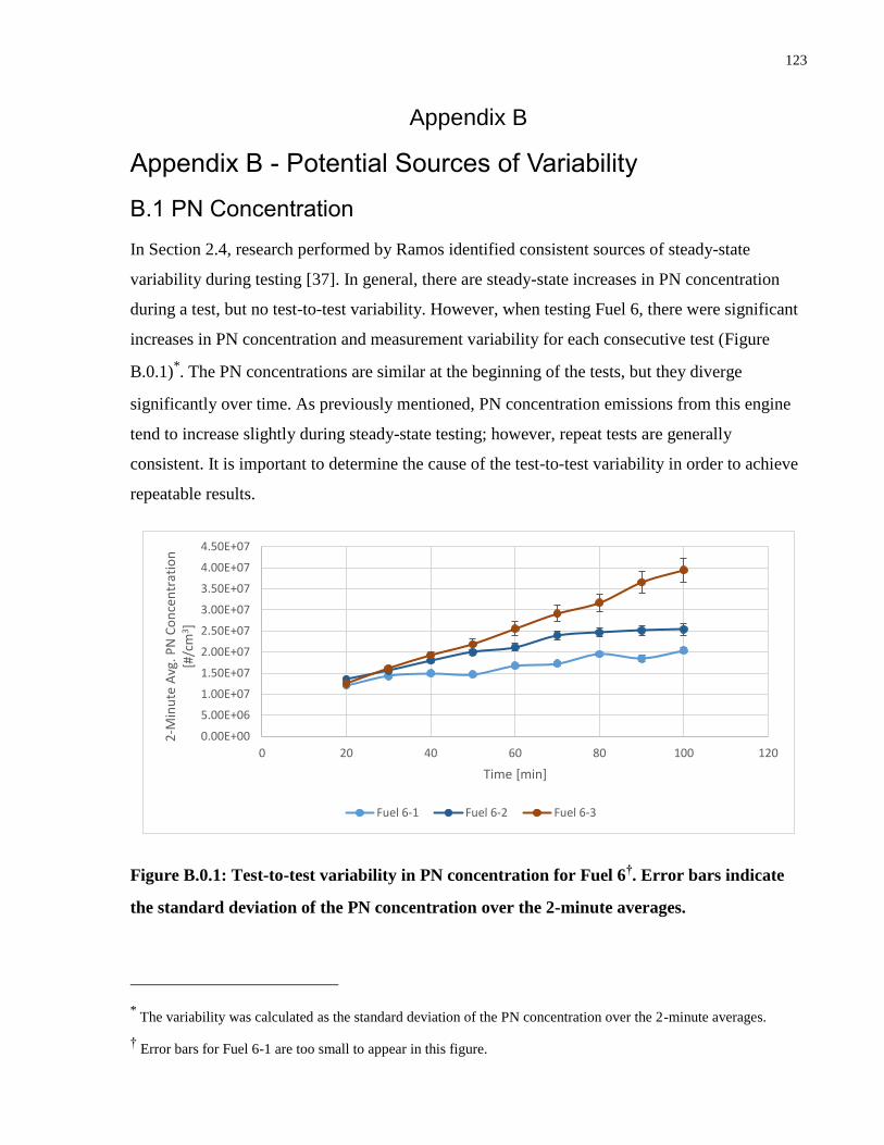
123

Appendix B

Appendix B - Potential Sources of Variability

B.1 PN Concentration

In Section 2.4, research performed by Ramos identified consistent sources of steady-state

variability during testing [37]. In general, there are steady-state increases in PN concentration

during a test, but no test-to-test variability. However, when testing Fuel 6, there were significant

increases in PN concentration and measurement variability for each consecutive test (Figure

B.0.1)*. The PN concentrations are similar at the beginning of the tests, but they diverge

significantly over time. As previously mentioned, PN concentration emissions from this engine

tend to increase slightly during steady-state testing; however, repeat tests are generally

consistent. It is important to determine the cause of the test-to-test variability in order to achieve

repeatable results.

Figure B.0.1: Test-to-test variability in PN concentration for Fuel 6†. Error bars indicate

the standard deviation of the PN concentration over the 2-minute averages.

* The variability was calculated as the standard deviation of the PN concentration over the 2-minute averages.

† Error bars for Fuel 6-1 are too small to appear in this figure.

0.00E+00

5.00E+06

1.00E+07

1.50E+07

2.00E+07

2.50E+07

3.00E+07

3.50E+07

4.00E+07

4.50E+07

0 20 40 60 80 100 120

2-M

inu

te A

vg. P

N C

on

cen

trat

ion

[#

/cm

3]

Time [min]

Fuel 6-1 Fuel 6-2 Fuel 6-3

124

The test-to-test variability was examined in terms of short term fuel trim (STFT), equivalence

ratio, and the Engine Exhaust Particle Sizer (EEPS). Six identical tests were performed using a

single batch of Shell 91 pump gasoline to examine the source of the test-to-test variability. These

tests are identified as: Shell 91-1, 91-2, 91-3, 91-4, 91-5, and 91-6 respectively. Figure B.0.2

illustrates that the variability observed with Fuel 6 is also present in the Shell 91 pump gasoline

tests; indicating that the variability is not a function of the fuel composition. It is important to

note the increase in variability at the end of the test compared to the beginning, and the increase

in variability for the tests ending at a higher PN concentration compared to those at lower PN

concentrations.

Figure B.0.2: Variability in Shell-91 pump gasoline tests. Error bars indicate the standard

deviation of the PN concentration over the 2-minute averages.

B.1.1 Short Term Fuel Trim and Equivalence Ratio

One potential cause of the test-to-test variability was the short-term fuel trim (STFT). The PCM

on this engine trims the fuel up (enrich) or down (lean-out) depending on the feedback from the

oxygen sensor in the engine exhaust. If the STFT remains at constant high or low values over

time, the PCM should adjust the long-term fuel trim (LTFT). However, the PCM used in this

study does not have the ability to store values in its memory. Between each test, the PCM reverts

to its default conditions, which disables the ability for LTFT [37].

0.00E+00

5.00E+06

1.00E+07

1.50E+07

2.00E+07

2.50E+07

0 20 40 60 80 100 120

2-M

nu

te A

vg. P

N C

on

cen

trat

ion

[#/

cm3 ]

Time [min]

Shell 91-1 Shell 91-2 Shell 91-3 Shell 91-4 Shell 91-5 Shell 91-6

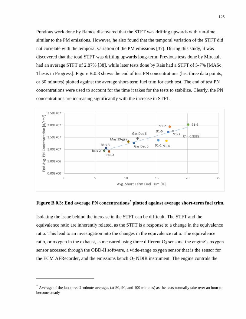
125

Previous work done by Ramos discovered that the STFT was drifting upwards with run-time,

similar to the PM emissions. However, he also found that the temporal variation of the STFT did

not correlate with the temporal variation of the PM emissions [37]. During this study, it was

discovered that the total STFT was drifting upwards long-term. Previous tests done by Mireault

had an average STFT of 2.87% [38], while later tests done by Rais had a STFT of 5-7% [MASc

Thesis in Progress]. Figure B.0.3 shows the end of test PN concentrations (last three data points,

or 30 minutes) plotted against the average short-term fuel trim for each test. The end of test PN

concentrations were used to account for the time it takes for the tests to stabilize. Clearly, the PN

concentrations are increasing significantly with the increase in STFT.

Figure B.0.3: End average PN concentrations* plotted against average short-term fuel trim.

Isolating the issue behind the increase in the STFT can be difficult. The STFT and the

equivalence ratio are inherently related, as the STFT is a response to a change in the equivalence

ratio. This lead to an investigation into the changes in the equivalence ratio. The equivalence

ratio, or oxygen in the exhaust, is measured using three different O2 sensors: the engine’s oxygen

sensor accessed through the OBD-II software, a wide-range oxygen sensor that is the sensor for

the ECM AFRecorder, and the emissions bench O2 NDIR instrument. The engine controls the

* Average of the last three 2-minute averages (at 80, 90, and 100 minutes) as the tests normally take over an hour to

become steady

91-1

91-2

91-3

91-4

91-5

91-6

Gas Dec 5

Rais-1

Gas Dec 6

May 29-gas

Rais-3

Rais-2

R² = 0.8383

0.00E+00

5.00E+06

1.00E+07

1.50E+07

2.00E+07

2.50E+07

0 5 10 15 20 25

End

Avg

. PN

Co

nce

ntr

atio

n [

#/cm

3 ]

Avg. Short Term Fuel Trim [%]

126

STFT using the reading from the engine’s oxygen sensor (OBD-II value), and the other two

sensors are used to confirm the OBD-II readings. In Table B.1, the readings from each of these

sensors can be seen from a variety of tests. Since the test-to-test PM emissions variability was a

fairly recent issue, older tests done in this investigation with 91 octane pump gasoline were used

(early-1 and early-2), as well as older tests done by Rais (Rais-1, 2, and 3) [MASc Thesis in

Progress], also with 91 octane pump gasoline. Note that the composition of the pump gasoline

used for the “early” and “Rais” tests was likely different than that of the current batch. Emissions

bench data is not available for Shell 91-1, 91-4, 91-5, and 91-6 tests, and will not be used in this

discussion.

Table B.1: Oxygen and equivalence ratio readings from gasoline testing.

E-bench O2 OBD-II sensor ECM sensor

%O2 Phi Phi

91-2 1.252083435 1.000799433 1.04373166

91-3 1.348990577 0.998957866 1.04506854

Rais-1 1.990806494 1.000238519 1.0136921

Rais-2 1.087419616 0.999669985 1.01414258

Rais-3 1.344144005 0.999732625 1.0143707

early-1 1.068672439 0.999544323 1.03702884

early-2 1.022481063 0.999386865 1.03744846

It is evident that either the OBD-II O2 sensor or the ECM AFRecorder O2 sensor is drifting. The

concentration of carbon monoxide (CO) in the exhaust is a good indicator of equivalence ratio

for rich mixtures, as it should increase with increasing equivalence ratio. Figure B.0.4 shows the

concentration of carbon monoxide measured by the emissions bench against the equivalence

ratio logged by the ECM AFRecorder. Clearly, the concentration of carbon monoxide is

increasing with the equivalence ratio. This indicates that the engine’s oxygen sensor (OBD-II

value) is erroneously drifting leaner than the actual value.

127

Figure B.0.4: Engine exhaust carbon monoxide concentration as a function of ECM

AFRecorder equivalence ratio*.

Since the OBD-II O2 sensor is always reading stoichiometric, it is likely that as the sensor is

drifting leaner, the engine is compensating by increasing the STFT. So the OBD-II would still

read stoichiometric; however, the ECM AFRecorder readings would reflect these STFT increases

and read rich. This is clear in Figure B.0.5, which displays the correlation between STFT and the

actual equivalence ratio.

* Shell 91-1, 91-4, 91-5, and 91-6 did not collect CO data due to the long calibration procedure for the emissions

bench, and to avoid unnecessary use of the calibration gases.

91-2

91-3

Rais-1Rais-2

Rais-3

early-1early-2

R² = 0.9896

0

1000

2000

3000

4000

5000

6000

7000

8000

9000

10000

1.01 1.015 1.02 1.025 1.03 1.035 1.04 1.045 1.05

Emis

sio

ns

Ben

ch C

O [

pp

m]

ECM AFRecorder Equivalence Ratio [Φ]

128

Figure B.0.5: Average short-term fuel trim plotted against the ECM AFRecorder

equivalence ratio.

To resolve this issue, a new OBD-II O2 sensor was installed on the engine to eliminate the drift.

With the new O2 sensor installed, the STFT reduced to approximately 10%, the ECM

AFRecorder equivalence ratio reduced to approximately 1.01, and the carbon monoxide

concentration reduced to approximately 6200 ppm. High CO concentrations were found for all

tests done before the O2 sensor was replaced. While the new O2 sensor fixed the enriching of the

air-fuel mixture, it did not have a significant effect on the test-to-test PM emissions variability.

B.1.2 Engine Exhaust Particle Sizer

The Engine Exhaust Particle Sizer (EEPS) is also another potential source of the variability. It is

possible that there is soot building up in the EEPS, and that this build-up is causing the

significant increases between each test. To test the measurement from the EEPS, the inlet line

coming from the rotating disk thermodiluter was replaced with a HEPA filter so that the EEPS

was just measuring filtered air. The inlet line was replaced intermittently through the test so that

the EEPS could record background measurements; in theory, the PN concentration should drop

to ambient levels during the intervals when the HEPA filter was connected in place of the diluter

outlet.

Figure B.0.6 shows the results from two gasoline tests: Test A, before EEPS electrometer

cleaning; and Test B, after cleaning. As can be seen in Figure B.0.7, there are significant

91-1

91-2

91-391-4

91-5

early-1Rais-1

Rais-3Rais-2

early-2

R² = 0.8343

0

5

10

15

20

25

1.01 1.015 1.02 1.025 1.03 1.035 1.04 1.045 1.05

Avg

. STF

T [%

]

ECM AFRecorderEquivalence Ratio [Φ]

129

increases in the PN concentration for Test A, which can be correlated with increases in the EEPS

background measurement. These increases were not found in Test B, indicating that there was a

build-up of particles in the EEPS electrometer column which caused an artificial increase in

emissions. Figure B.0.6 and Figure B.0.7 show the impact of cleaning: the PN concentration for

Test B is steady, and the EEPS background measurements remain at an ambient level. The

increase in variability during a test can also be seen by the increased error in Figure B.0.1 and

Figure B.0.2. To reduce systematic variability, the EEPS will be cleaned regularly: soot will be

removed from the negative and positive charger needles and the electrometers will be cleaned

with acetone and regularly zeroed. Furthermore, the dilution ratio will be increased from 80 to

105, which will decrease the number of particles travelling through the analyzer and reducing the

need for cleaning.

Figure B.0.6: Comparison of two gasoline tests: before (Test A) and after (Test B) EEPS

cleaning.

0

100000

200000

300000

400000

500000

600000

700000

0 10 20 30 40 50 60 70 80 90 100

Raw

PN

Co

nce

ntr

atio

n [

#/cm

3]

Time (min)Test A Test B

130

Figure B.0.7: Comparison of two EEPS background readings: before (Test A) and after

(Test B) EEPS cleaning.

While cleaning the EEPS reduced the test-to-test variability, the issue of variability within a test,

as shown in Figure B.0.1 and Figure B.0.2, persisted. Originally, the variability was only

observed in terms of PN concentration for Fuel 6; however, in Figure B.0.8 it is evident that

there were also increases in PM mass over the duration of a test. The increase in both PN

concentration and PM mass confirms that there is an actual change in engine emissions, and not

solely a measurement issue.

0

10000

20000

30000

40000

50000

60000

0 10 20 30 40 50 60 70 80 90 100Raw

PN

Co

nce

ntr

atio

n [

#/cm

3 ]

Time (min)

Test A Test B

131

Figure B.0.8: Test variability in PM mass for Fuels 5, 6, 7, 8, 9, 10, and 11. Error bars

indicated standard deviation for all filters within the specified range

This section has shown that a number of operational issues arose with both the engine and

measurement instruments that resulted in increased measurement variability between tests.

Those issues were investigated and fixed as they arose and had no impact on the data sets that

will be discussed in Section 5.1. The long-standing issue of rising PN (and PM mass) emissions

with increasing run time has not been resolved but is consistent and therefore allows

comparisons between fuels.

B.2 Engine Parameters

In order to isolate the effects of fuel composition, it is important to analyze the engine

parameters and confirm that any changes did not affect the engine out emissions*.

B.2.2 Engine Exhaust Temperature

The engine exhaust temperature is a good marker for in-cylinder combustion temperature. From

examining Figure B.0.9 and Figure B.0.10, it is clear that the combustion temperature had little

effect on the engine PM emission or THC emissions. One thing to note is the low combustion

* CO has already been shown to change dramatically due to the O2 sensor replacement.

0

2

4

6

8

10

12

14

16

18


PM

mas

s [m

g/m

3 ]

Test

Early tests Late tests

132

temperatures for Fuels 1, 2, and 3. Interestingly, Fuels 1R, 4, and one test of Fuel 12 have higher

exhaust temperatures. At this time there is no explanation for why there is this difference, but it

is clear that it did not have a significant effect on the PN concentration or the THC emissions.

Figure B.0.9: End Average PN Concentration plotted against Pre-Catalyst Exhaust

Temperature.

Figure B.0.10: Emissions bench THC plotted against Pre-Catalyst Exhaust Temperature

Figure B.0.11 shows an interesting relationship between the pre-catalyst exhaust temperature

(closest to the engine), and the post-sample exhaust temperature (farthest from the engine). It

0

5000000

10000000

15000000

20000000

25000000

635 640 645 650 655 660End

Avg

. PN

Co

ncn

etra

tio

n [

#/cm

3 ]

Pre-catalyst Exhaust Temperature [°C]



0

200

400

600

800

1000

1200

1400

1600

635 640 645 650 655 660

Emis

sio

ns

Ben

ch T

HC

[p

pm

C3]

Pre-Catalyst Exhaust Temperature [°C]



133

seems as though these temperatures should be closely linked, as nothing else is changing

between them; however, the post-sample exhaust temperature seemingly increased consistently

from around Fuel 5 until Fuel 12. It is interesting to note the differences in post-sample

temperature between Fuel 1 and 1R, and the difference between the latter two tests of Fuel 3 and

the earlier one. As nothing has changed regarding the exhaust pipe, it is possible that the post-

sample thermocouple has drifted and is reading incorrect temperatures. In either situation, the

temperature increase has not resulted in any change in emissions.

Figure B.0.11: Post-Sample Exhaust Temperature plotted against Pre-Catalyst Exhaust

Temperature

B.2.3 Equivalence Ratio

As previously mentioned, the exhaust O2 sensor was replaced between Fuels 6 and 7 of this

investigation. This was found by examining the tests prior to the sensor replacement, and finding

that they had elevated CO values compared to historical measurements with this engine and

equipment. It is important to ensure that the sensor did not have any drastic effects on other

engine emissions.

Figure B.0.12 and Figure B.0.13 plot emissions bench NOx and THC respectively against the

AFRecorder Equivalence Ratio. While the NOx shows little trend, it seems as though the THC

values were higher prior to the sensor replacement. This is especially obvious when looking at

315

320

325

330

335

340

345

350

635 640 645 650 655 660

Po

st-S

amp

le E

xhau

st T

emp

erat

ure

[°C

]

Pre-Catalyst Exhaust Temperature [°C]

134

Fuels 1 and 1R, and the early Fuel 3 test compared to the latter two. Furthermore, the high

equivalence ratio group is visibly higher than the post-O2 sensor replacement group.

Figure B.0.12: Emissions bench NOx plotted against AFRecorder Equivalence Ratio

Figure B.0.13: Emissions bench THC plotted against AFRecorder Equivalence Ratio

B.2.4 Engine Load

Finally, the engine load was examined to determine if changes in load were affecting the engine

out emissions. To more closely examine this, Figure B.0.14 and Figure B.0.15 display the end

0

500

1000

1500

2000

2500

3000

1.005 1.01 1.015 1.02 1.025 1.03 1.035 1.04 1.045

Emis

sio

ns

Ben

ch N

Ox [p

pm

]

AFRecorder Equivalence Ratio [Ø]

Fuel 1 Fuel 1R Fuel 2 Fuel 3 Fuel 4 Fuel 5 Fuel 6 Fuel 7 Fuel 8 Fuel 10 Fuel 11 Fuel 12

0

200

400

600

800

1000

1200

1400

1600

1.005 1.01 1.015 1.02 1.025 1.03 1.035 1.04 1.045

Emis

sio

ns

Ben

ch T

HC

[p

pm

C3]

AFRecorder Equivalence Ratio [Ø]



135

average PN concentrations plotted against the load for the high PN and low PN groups,

respectively. There is no correlation for either of the PN groups. While Fuels 5 and 6 had slightly

lower engine loads, it did not affect the PN concentrations. If the load was affecting emissions,

there should be an increase in emissions with higher load, not a decrease.

Figure B.0.14: End Average PN Concentration for the high PN fuels plotted against engine

load

Figure B.0.15: End Average PN Concentration for the low PN fuels plotted against engine

load

0

5000000

10000000

15000000

20000000

25000000

37 37.5 38 38.5 39 39.5 40 40.5 41 41.5 42 42.5

End

Avg

. PN

Co

nce

ntr

atio

n [

#/cm

3 ]

Load [lb-ft]

Fuel 5 Fuel 6 Fuel 7 Fuel 8 Fuel 9 Fuel 10 Fuel 11 Fuel 12

0

200000

400000

600000

800000

1000000

1200000

38 38.5 39 39.5 40 40.5 41 41.5 42 42.5 43

End

Avg

. PN

Co

nce

ntr

atio

n [

#/cm

3]

Load [lb-ft]

Fuel 1 Fuel 1R Fuel 2 Fuel 3 Fuel 4 Fuel 12

136

B.3 PM Mass Measurements

It is important to note the relatively high masses of Fuels 1, 2, and 3 compared to their PN

concentrations. Figure B.0.16 shows the actual filters taken during these tests, which all have

similar PM masses, approximately 3 mg/m3. While it may be difficult to see in the photos, the

filter for Fuel 11-1 is noticeably darker than the other two, indicating it collected more mass

during testing. Interestingly, while all three filters for Fuels 11-1, 2, and 1-2, collected mass for

the same amount of time (10 minutes), they had dilution ratios of 93, 25, and 24, respectively.

Due to their high DR, it is expected that at equal PM masses, the filters for Fuel 2 and 1-2 should

have far more actual mass collected on the filters compared to Fuel 11-1. Since this did not

happen, it is possible that the recorded PM mass for Fuels 1, 2, and 3 are incorrect. Figure B.0.17

illustrates the dichotomy between the early and late measurements. The low PM mass

measurements agree with the PN concentrations, and ultimately are more likely to be accurate

based on the filter photos. Unfortunately, due to the high DR during later tests, there are not

many good data points for Fuels 1 and 3, and no data points for Fuel 2. For the PM masses

presented in this investigation, the Fuel 1R and 3R filters will be used, and Fuel 2 PM masses will

be removed from all analysis.

Figure B.0.16: From left to right: Fuel 11-1 early filter, Fuel 2 early filter, and Fuel 1-2

early filter.

137

Figure B.0.17: End average PN concentrations plotted against PM masses for low PN fuels

and Fuel 11-1.

Fuel 3-1Fuel 3R-1

Fuel 3R-2

Fuel 12-1

Fuel 12-2

Fuel 12-3

Fuel 1-1 Fuel 1-2

Fuel 1R-3 Fuel 1-3

Fuel 11-1

Fuel 2

10000

100000

1000000

10000000

0 0.5 1 1.5 2 2.5 3 3.5 4

End

Avg

. PN

Co

nce

ntr

atio

n [

#/cm

3 ]

PM Mass [mg/m3]

138

Appendix C

Appendix C - Calculations

C.1 PN Index

For this study, the PN Index calculations are based off of previous work by Ramos, which was a

simplified version of the procedure presented by Leach et al. [37, 33]. To simplify the

calculations, Raoult’s law was used to calculate the vapour pressure (DVPE) of the fuel, instead

of the more complicated UNIFAC method used by Leach et al. [33].

In Table C.1, the fuel properties needed to calculate the PN Index for all the fuel blends are

listed. The molecular weight, DBE value, and density of all the fuels can be found in the product

specifications, listed in Table 3.8. The vapour pressures for all the components except the

solvents, were found in the US EPA’s compilation of air emissions factors [87]. The calculations

for the PN Index are shown below.

Table C.1: Properties needed for PN Index for components used in fuel blends.

Boiling Point (K)

RVP (kPa)

Molecular Weight

DBE+1 Density (kg/m3)

Density (kg/L)

Isooctane 372 4.11 114.23 1 690 0.69

Toluene 384 6.94 92.14 5 867 0.87

Pentane 309 106.69 72.15 1 626 0.63

Hexane 341 33.73 86.18 1 655 0.66

Xylene 411.5 2.41 106.16 5 861 0.86

Naphthalene 491 0.09 128.17 8 1140 1.14

Solvent #1 437 0.47 127.21 5 880 0.88

Solvent #2 465 0.40 148.24 5 898 0.90

Thiophene 357

84.14 4 1050 1.05

For xylene and naphthalene, no direct vapour pressure was found in the EPA report. However,

Equation C.1 was provided to calculate the vapour pressure:

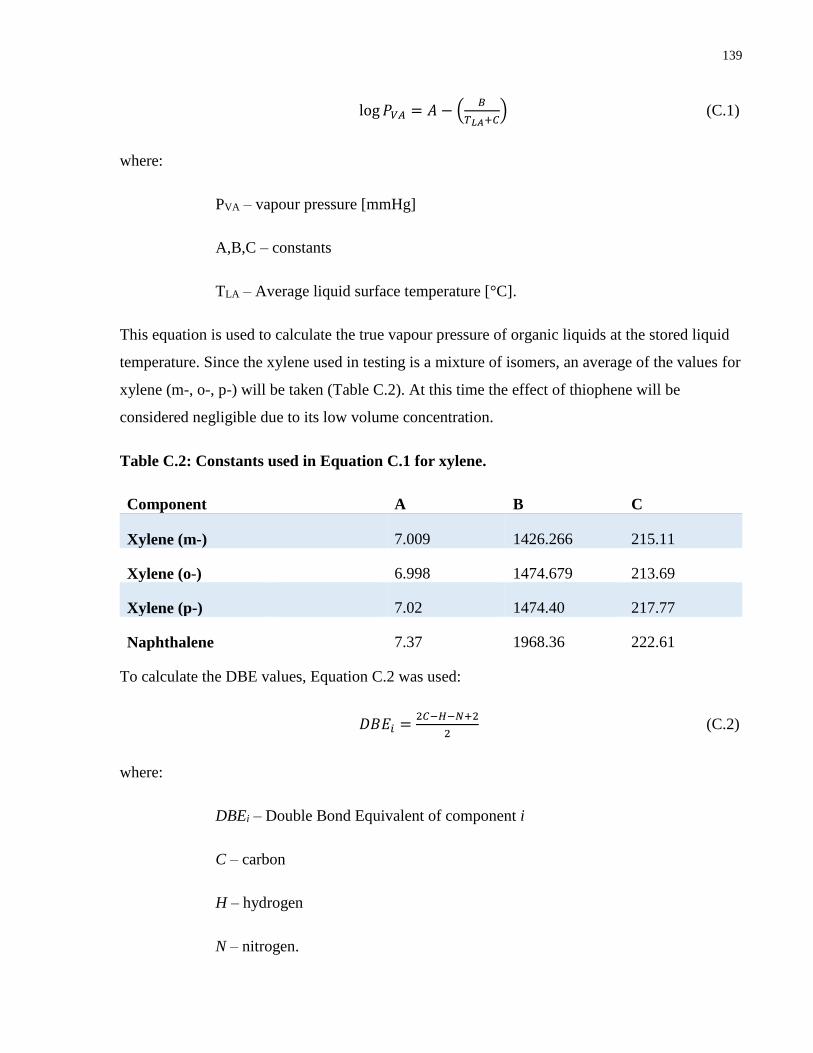
139

log 𝑃𝑉𝐴 = 𝐴 − (𝐵

𝑇𝐿𝐴+𝐶) (C.1)

where:

PVA – vapour pressure [mmHg]

A,B,C – constants

TLA – Average liquid surface temperature [°C].

This equation is used to calculate the true vapour pressure of organic liquids at the stored liquid

temperature. Since the xylene used in testing is a mixture of isomers, an average of the values for

xylene (m-, o-, p-) will be taken (Table C.2). At this time the effect of thiophene will be

considered negligible due to its low volume concentration.

Table C.2: Constants used in Equation C.1 for xylene.

Component A B C

Xylene (m-) 7.009 1426.266 215.11

Xylene (o-) 6.998 1474.679 213.69

Xylene (p-) 7.02 1474.40 217.77

Naphthalene 7.37 1968.36 222.61

To calculate the DBE values, Equation C.2 was used:

𝐷𝐵𝐸𝑖 =2𝐶−𝐻−𝑁+2

2 (C.2)

where:

DBEi – Double Bond Equivalent of component i

C – carbon

H – hydrogen

N – nitrogen.

140

The DBE values for the two solvents needed to be approximated, as they are made up of a blend

of hydrocarbons. Solvent #1 has an aromatic content greater than 99% and consists of primarily

C9-C10 dialkyl and trialkylbenzenes. Furthermore Solvent #2 is also approximately 99%

aromatics and is composed primarily of C10-C12 alkyl benzenes. As both of the blends are made

up of mostly benzene structures, it can be reasonably assumed that their DBE values are

approximately 4 [88].

In addition, the molecular weights for the two solvents were approximated by averaging the

molecular weights of each benzene structure at the associated carbon numbers. So Solvent #1

and Solvent #2 had weighted averages for C9-C10 and C10-C12, respectively. The molecular

formulas are calculated using benzenes alkyl derivatives: C6H5 CnH2n+1 [89].

To calculate the mole fraction, Equation C.3 was used:

𝑛𝑖 =𝑉𝑖∗𝜌𝑖

𝑀𝑖 (C.3)

where:

Vi – Volume fraction of each component i

ρi – density of each component i

Mi – molar mass of each component i.

To calculate the DVPE, Equation C.4 was used:

𝐷𝑉𝑃𝐸 = ∑ (𝑅𝑉𝑃𝑖 ∗ 𝑥𝑖)𝑛𝑖=1 (C.4)

where:

RVPi – Reid Vapour Pressure of each component i

xi – mole fraction of each component i.

141

To calculate the DBE+1 value,

𝐷𝐵𝐸 + 1𝑖 = ∑ (𝐷𝐵𝐸𝑖 + 1) ∗ 𝑉𝑖𝑛𝑖=1 (C.5)

Finally, to calculate the PN Index, Equation 2.2 from Chapter 2 is used:

PN Index =∑ [𝐷𝐵𝐸𝑖+1]𝑉𝑖

ni=1

DVPE (kPa) (C.6)

C.2 Emissions Bench

Water content in the exhaust must be calculated using the concentration of CO and CO2 in the

exhaust, as well as the number of carbon and hydrogen atoms in the fuel. Dry NOx is calculated

using the wet NOx values and the calculated H2O values.

Both equations for the H2O content (C.7) and dry NOx (C.8) are from Heywood [53]:

�̃�𝐻2𝑂 =𝑚

2𝑛[

�̃�𝐶𝑂∗ +�̃�𝐶𝑂2

∗

1+�̃�𝐶𝑂

∗

𝐾∗�̃�𝐶𝑂2∗ +(

𝑚

2𝑛)(�̃�𝐶𝑂

∗ +�̃�𝐶𝑂2∗ )

] (C.7)

where:

�̃�𝐻2𝑂 – calculated water mole fraction

�̃�𝐶𝑂∗ – dry CO mole fraction

�̃�𝐶𝑂2

∗ – dry CO2 mole fraction

m, n – carbon and hydrogen atoms in the fuel (CnHm)

𝐾 – empirical constant assumed to be 3.8 [37, 53].

142

�̃�𝑁𝑂𝑥

∗ =�̃�𝑁𝑂𝑥

1−�̃�𝐻2𝑂 (C.8)

where:

x̃NOx – wet NOx mole fraction

x̃H2O – calculated water mole fraction.

The O2 value measured by the emissions bench needs to be corrected. The NDIR measures O2 by

paramagnetic measuring that is based on oxygens high magnetic susceptibility. While most other

gases have insignificant susceptibility, the gases in Table C.3 are slightly higher. Thus, the O2

will be corrected for the exhaust constituents with the largest effect in this investigation.

Equation C.9 is from the correction procedure developed by CAI [90], and the correction values

are taken from Table C.3:

�̅�𝑂2

∗ = �̃�𝑂2

∗ − [−0.29

100∗�̃�𝐶𝑂2∗ −

0.07

100∗�̃�𝐶𝑂∗ +

43

100∗�̃�𝑁𝑂𝑥∗ ] (C.9)

where:

�̅�𝑂2

∗ – corrected dry mole fraction of O2

�̃�𝑂2

∗ - dry O2 mole fraction

�̃�𝐶𝑂2

∗ - dry CO2 mole fraction

�̃�𝐶𝑂∗ - dry CO mole fraction

�̃�𝑁𝑂𝑥

∗ - calculated dry NOx mole fraction.

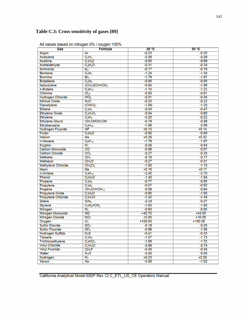
143

Table C.3: Cross sensitivity of gases [89]

144

C.3 Dilution Ratio

The calculation for the dilution has not changed from the procedure used by Ramos [37], and

will be repeated verbatim. The calculation is based off the difference between the raw exhaust

CO2 measured by the emissions bench, and the diluted exhaust CO2 measured by the LI-COR

CO2 monitor.

Conservation of Mass: assume a control volume around diluter, with raw exhaust and dilution air

coming in, and diluted exhaust coming out.

�̇�𝑒𝑥ℎ𝑎𝑢𝑠𝑡𝑑𝑖𝑙𝑢𝑡𝑒𝑑= �̇�𝑒𝑥ℎ𝑎𝑢𝑠𝑡𝑟𝑎𝑤

+ �̇�𝑑𝑖𝑙𝑢𝑡𝑖𝑜𝑛 𝑎𝑖𝑟 (C.10)

Conservation of Species: assume no CO2 is destroyed or generated during dilution.

�̇�𝐶𝑂2𝑒𝑥ℎ𝑎𝑢𝑠𝑡𝑑𝑖𝑙𝑢𝑡𝑒𝑑= �̇�𝐶𝑂2𝑒𝑥ℎ𝑎𝑢𝑠𝑡𝑟𝑎𝑤

+ �̇�𝐶𝑂2𝑑𝑖𝑙𝑢𝑡𝑖𝑜𝑛 𝑎𝑖𝑟 (C.11)

where:

�̇�𝐶𝑂2𝑒𝑥ℎ𝑎𝑢𝑠𝑡𝑑𝑖𝑙𝑢𝑡𝑒𝑑= �̇�𝑒𝑥ℎ𝑎𝑢𝑠𝑡𝑑𝑖𝑙𝑢𝑡𝑒𝑑

∗ 𝑥𝐶𝑂2𝑒𝑥ℎ𝑎𝑢𝑠𝑡𝑑𝑖𝑙𝑢𝑡𝑒𝑑 (a)

�̇�𝐶𝑂2𝑒𝑥ℎ𝑎𝑢𝑠𝑡𝑟𝑎𝑤= �̇�𝑒𝑥ℎ𝑎𝑢𝑠𝑡𝑟𝑎𝑤

∗ 𝑥𝐶𝑂2𝑒𝑥ℎ𝑎𝑢𝑠𝑡𝑟𝑎𝑤 (b)

�̇�𝐶𝑂2𝑑𝑖𝑙𝑢𝑡𝑖𝑜𝑛 𝑎𝑖𝑟 = �̇�𝑑𝑖𝑙𝑢𝑡𝑖𝑜𝑛 𝑎𝑖𝑟 ∗ 𝑥𝐶𝑂2𝑑𝑖𝑙𝑢𝑡𝑖𝑜𝑛 𝑎𝑖𝑟 (c)

Combination of equations and rearranging:

Combine Equation C.11 with Equations (a), (b), and (c):

�̇�𝑒𝑥ℎ𝑎𝑢𝑠𝑡𝑑𝑖𝑙𝑢𝑡𝑒𝑑∗ 𝑥𝐶𝑂2𝑒𝑥ℎ𝑎𝑢𝑠𝑡𝑑𝑖𝑙𝑢𝑡𝑒𝑑

= �̇�𝑒𝑥ℎ𝑎𝑢𝑠𝑡𝑟𝑎𝑤∗ 𝑥𝐶𝑂2𝑒𝑥ℎ𝑎𝑢𝑠𝑡𝑟𝑎𝑤

+ �̇�𝑑𝑖𝑙𝑢𝑡𝑖𝑜𝑛 𝑎𝑖𝑟 ∗ 𝑥𝐶𝑂2𝑑𝑖𝑙𝑢𝑡𝑖𝑜𝑛 𝑎𝑖𝑟

(C.12)

Rearranging Equation C.12:

𝑥𝐶𝑂2𝑒𝑥ℎ𝑎𝑢𝑠𝑡𝑑𝑖𝑙𝑢𝑡𝑒𝑑=

�̇�𝑒𝑥ℎ𝑎𝑢𝑠𝑡𝑟𝑎𝑤∗𝑥𝐶𝑂2𝑒𝑥ℎ𝑎𝑢𝑠𝑡𝑟𝑎𝑤+�̇�𝑑𝑖𝑙𝑢𝑡𝑖𝑜𝑛 𝑎𝑖𝑟∗𝑥𝐶𝑂2𝑑𝑖𝑙𝑢𝑡𝑖𝑜𝑛 𝑎𝑖𝑟

�̇�𝑒𝑥ℎ𝑎𝑢𝑠𝑡𝑑𝑖𝑙𝑢𝑡𝑒𝑑

(C.13)

Sub Equation C.10 into C.13:

145


�̇�𝑒𝑥ℎ𝑎𝑢𝑠𝑡𝑟𝑎𝑤∗𝑥𝐶𝑂2𝑒𝑥ℎ𝑎𝑢𝑠𝑡𝑟𝑎𝑤+( �̇�𝑒𝑥ℎ𝑎𝑢𝑠𝑡𝑑𝑖𝑙𝑢𝑡𝑒𝑑−�̇�𝑒𝑥ℎ𝑎𝑢𝑠𝑡𝑟𝑎𝑤)∗𝑥𝐶𝑂2𝑑𝑖𝑙𝑢𝑡𝑖𝑜𝑛 𝑎𝑖𝑟


(C.14)

Multiply out Equation C.14 and collect like terms:


�̇�𝑒𝑥ℎ𝑎𝑢𝑠𝑡𝑟𝑎𝑤


∗ (𝑥𝐶𝑂2𝑒𝑥ℎ𝑎𝑢𝑠𝑡𝑟𝑎𝑤− 𝑥𝐶𝑂2𝑑𝑖𝑙𝑢𝑡𝑖𝑜𝑛 𝑎𝑖𝑟) + 𝑥𝐶𝑂2𝑑𝑖𝑙𝑢𝑡𝑖𝑜𝑛 𝑎𝑖𝑟 (C.15)

Solve for Dilution Ratio:

𝐷𝑖𝑙𝑢𝑡𝑖𝑜𝑛 𝑅𝑎𝑡𝑖𝑜 =�̇�𝑒𝑥ℎ𝑎𝑢𝑠𝑡𝑟𝑎𝑤


=𝑥𝐶𝑂2𝑒𝑥ℎ𝑎𝑢𝑠𝑡𝑟𝑎𝑤−𝑥𝐶𝑂2𝑑𝑖𝑙𝑢𝑡𝑖𝑜𝑛 𝑎𝑖𝑟

𝑥𝐶𝑂2𝑒𝑥ℎ𝑎𝑢𝑠𝑡𝑑𝑖𝑙𝑢𝑡𝑒𝑑−𝑥𝐶𝑂2𝑑𝑖𝑙𝑢𝑡𝑖𝑜𝑛 𝑎𝑖𝑟

(C.16)

C.4 Effective Particle Density

To calculate the effective density of the particles in this investigation, the PM mass, the PN

concentration, and the mobility diameter of the particles was used. Initially, the mobility

diameter was calculated by taking a weighted average of the PN size distribution, as shown in

Equation C.15:

𝑑𝑝,𝑎𝑣𝑔 = ∑ 𝑑𝑝,𝑖 ∗ (∗ 𝑜𝑓 𝑝𝑎𝑟𝑡𝑖𝑐𝑙𝑒𝑠)𝑖523.3𝑖=6.04 (C.15)

where:

𝑑𝑝,𝑎𝑣𝑔 – average mobility diameter for the fuel tested

𝑑𝑝,𝑖 – mobility diameter for the EEPS channel

(∗ 𝑜𝑓 𝑝𝑎𝑟𝑡𝑖𝑐𝑙𝑒𝑠)𝑖 – number of particles counted in that bin.

Following this, the average volume of the particles was calculated using the average mobility

diameter, using Equation C.16:

146

𝑉𝑝,𝑎𝑣𝑔 =4

3∗ 𝜋 ∗ [

𝑑𝑝,𝑎𝑣𝑔

2]

3

(C.16)

where:

𝑉𝑝,𝑎𝑣𝑔 – Average volume of the particles

𝑑𝑝,𝑎𝑣𝑔 – average mobility diameter for the fuel tested.

Finally, the effective particle density is calculated using Equation C.17 below:

𝜌𝑒𝑓𝑓 =[

𝑃𝑀 𝑚𝑎𝑠𝑠

𝑃𝑁 𝑐𝑜𝑛𝑐]

𝑉𝑝,𝑎𝑣𝑔 (C.17)

where:

𝜌𝑒𝑓𝑓 – effective particle density

PM mass – measured particle mass

PN conc – measured PN concentration

𝑉𝑝,𝑎𝑣𝑔 – Average volume of the particles.

Effect of Fuel Composition on Particulate Matter Emissions ...

Documents

Transcript of Effect of Fuel Composition on Particulate Matter Emissions ...