EFFECT OF CHARGE WEIGHT ON VIBRATION LEVELS FROM QUARRY BLASTING

By James F. Devine, Richard H. Beck, Alfred V. C. Meyer, and Wilbur I. Duvall

• • • • • • • • • • • report of investigations 6774

www.ARblast.osmre.QOV ·

US Department of Interior Office of Surface Mining Reclamation and Enforcement

Kenneth K. Eltschlager

UNITED STATES DEPARTMENT OF THE INTERIOR Stewart L. Udall, Secretary

BUREAU OF MINES Walter R. Hibbard, Jr., Director

Mining/Explosives Engineer 3 Parkway Center

Pittsburgh, PA 15220 Office: 412.937.2169

Cell: 724.263.8143 Keltschlaqer®osmre.qov

This publication has been cataloged as follows:

Devine, James F Effect of charge weight on vibration levels from quarry

blasting, by James F. Devine [and others. Washington] U.S. Dept. of the Interior, Bureau of Mines [1966]

37 p. illus., tables. (U.S. Bureau of Mines. Report of investiga•

tions 6774)

Includes bibliography.

1. Blasting. I. Title. II. Title: Quarry blasting. (Series)

TN23.U7 no. 6774 622.06173

U.S. Dept. of the Int. Library

•

CONTENTS

Abstract. ..•..... ;....................................................... 1 Introduction............................................................ 1 Acknowledgments. • . • . . . . . . . • . . • . . . . . • • . . • • . • • . • . . • • . . • • . . • . . • . • • . . . . • . • • • 2 Test sites ...••••••••.•••..•••• , •.. ,.................................... 2 Instrumentation and experimental procedures............................. 3 Experimental data ...•• , •. , ............. ,., .•.... , ........... ,........... 6 Data analysis ................................ ;.......................... 16 Application of the scaled propagation equation.......................... 30 Conclusions ...•.•....• , , •.. , , , , • , , , , , , . , . , , , ... , , , . , , .. , •.....•. , .•. , , , . 35 References.,., ..... ,,., •••. ,, ..... ,., ... ,,, .•.. , ...... ,,,,, •.. ,,,....... 37

Fig.

1. 2. 3. 4. 5. 6. 7. 8. 9.

10.

11.

12. 13. 14.

15.

ILLUSTRATIONS

Plan view of Iowa test site ...................... ·.- ............... .. Plan view of Washington, D.C., test site ......................... .. Plan view of New York test site .................. · ................. , Plan view of Ohio test site ...• , ..... , .. , .. ,,,, ... '.,., .... ,,, .... . Plan view of Virginia test site ............... ,. .................. . Peak particle velocity versus distance, radial component .......... . Peak particle velocity versus distance, vertical component ........ . Peak particle velocity versus distance, transverse component ...... . Particle velocity intercepts versus charge weight per delay,

radial component .. , .......... , ..... , ....... , , . , . , , . , .. , .... , ... , , Particle velocity intercepts versus charge weight per delay,

vertical component . ............................................. . Particle velocity intercepts versus charge weight per delay,

transverse component . .. , ........................................ . Peak particle velocity versus scaled distance, radial component ... . Peak particle velocity versus scaled distance, vertical component .. Peak particle velocity versus scaled distance, transverse

component . ...................................................... . Peak particle velocity versus scaled distance, combined data ......•

TABLES

4 5 5 7 7

18 19 20

24

25

26 31 32

33 34

1. Quarry blast data.................................................. 8 2, Particle velocity and frequency data for the Iowa sj.te ...• , , . , .. , • , 9 3. Particle velocity and frequency data for the D.C. s '· te. , ... , , ... , . , 11

\ '

ii

TABLES--Continued

4. Particle velocity and frequency data for the New York site......... 12 5. Particle velocity and frequency data for the Ohio site............. 13 6. Particle velocity and frequency data for the Virginia site lin<c 1.. 14 7. Particle vefcii:Hy aiiii Frequency -diit'i3. for tlie Virgihl.a _site line 2.. 16 8. Statistical tests for particle velocity versus distance data........ 21 9. Surmnary of K1 l' ai31 _and H1 data .............. _...................... 23

10. Statistical test for (K!J )l/13, versus W1 ;.......................... 27

11. Statistical tests for comparison of slope a with theoretical value of 1/2.. .. . .. . . . . .. . . . . . . . . . . . . . . . . .. . . . . . . . . . . . . . . . . . . . . . . . .. .. . 28

12. Summary of normalizing constants................................... 29

13. Statistical tests for (K!J)l/i3, I (H 1 ) 1 113, versus W1 J .............. 30

14. Summary of statistical tests for scaled and unsealed velocity-distance data.................................................... 30

15. Representative charge weight-distance relationships for scaled ' distance of 50 ft/lb'>.................................... ... . . . . . . 35

EFFECT OF CHARGE WEIGHT ON VIBRATION LEVELS FROM QUARRY BLASTING

by

James F. Devine, 1 Richard H. Beck, 1 Alfred V. C. Meyer, 2

and Wilbur I. Duvall 3

ABSTRACT

The radial, vertical, and tranSverse components of particle velocity were recorded by Bureau of Mines investigators along gage arrays extending in one or two directions for 145 to 3,170 feet at five quarrys. Of the 39 quarry blasts, 12 were instantaneous blasts, 5 were of the one hole per delay type, using millisecond delayed caps, and 22 were multiple hole per delay type employing millisecond delay detonating fuse connectors. Charge weight per hole ranged from 8 to 1,500 pounds, and the charge weight per delay interval, including the instantaneous blasts, ranged from 25 to 4,620 pounds.

Statistical analysis of the particle velocity-distance data shows that the square root of the charge weight per delay interval can be used as a scal­ing factor in a propagation equation of the form

where Vis the peak particle velocity produced at a distance, D, by a quarry blast of charge weight per delay interval, W, and HandS are constants for each component of velocity for each quarry site.

INTRODUCTION

Previous Bureau of Mines investigations of vibrations from instantaneous and millisecond delayed quarry blasts (~-~4 showed that the radial, vertical,

1 Research geophysicist, Denver Mining Research Center, College Park Field Office, Bureau of Mines, College Park, Md.

2 Geophysicist, Denver Mining Research Center, College Park Field Office, Bureau of Mines, College Park, Md.

3 Supervisory research physicist, Denver Mining Research Center, Bureau of Mines, Denver, Colo.

4 Underlined numbers in parentheses refer to items in the list of references at the end of this report.

Work on manuscript completed August 1965.

2

and_ transverse components of the peak particle velocity of ground vibrations could be represented by an equation of the form

V = HWbD-[l, (1)

where V is the peak particle velocity, W is the charge weight per delay inter­val or total charge weight for an instoanta·neous blast, D is the Eli&ta-nee f-rem blast area, and H, b, and S are constants far· a given site and component. Equation 1 for any one component implies that H, b, and ~ are independent parameters that have ,to be determined for each quarry site and shooting pro­cedure. Therefore, three constants must be determined before equation 1 can be used for predictions of vibration levels.

Equation 1 that the charge sealing factor.

where

is simplified if a relationship exists between b and ~ such weight per delay interval, W, raised to some power, a, is a

For this condition, equation 1 becomes:

a = b/~.

(2)

(3)

To determine the applicability of equation 2 to particle velocity-distance data requires a large amount of data from different sites which have different propagation parameters H, b, and S. Statistical methods can then be used to dete~ine if W0 is a scaling factor and, if so, to determine the value of a.

This Bureau of Mines report presents a summary of propagation data for the radial, vertical, and transverse components of the peak particle veloci­ties of ground vibrations produced by millisecond-delayed or instantaneous quarry blasts. Data from 39 blasts at five quarries, where the maximum charge weight per delay interval is accurately known, are included. The maximum charge weight per delay interval for these blasts ranges from 25 to 4,620 pounds. The particle velocity data were obtained for a distance range from 145 to 3,170 feet from the blast area.

ACKNOWLEDGMENTS

The authors wish to express their appreciation to the following companies for permitting the blasting tests at their quarries: Weaver Construction Company, Alden, Iowa; Northern Ohio Stone Company, Flat Rock, Ohio; New York Traprock Company, Clinton Point, N.Y.; and the Chemstone Corporation, Strasburg, Va. They also wish to thank Charles Croker, blasting consultant, and the Ohio Valley Construction Company for their cooperation in conducting the Washington, D.C. tests.

TEST SITES

The Iowa site is located at a quarry in central Iowa, near the town of Alden. The rock exposed at the face of this quarry is a light tan, argilla­ceous, loosely jointed limestone of the Gilmore City formation. The upper 10

3

feet exhibits weathering and crossbedding effects. There is virtually no structural dip in this area. The overburden, in which the gages were mounted, consists of 6 to 12 feet of black reworked· glacial till.

The Washington, D.C., site was located at the east approach of the Theodore Roosevelt Bridge over the Potomac River. The rock is dark greenish­gray gneissoid diorite with hornblende. The surface of the bedrock sloped eastward away from the blast area. The arenaceous clay overburden, which was approximately 5 feet thick at the working area, increased to approximately 40 to 50 feet thick at station 7 of the gage array.

The third site was in a quarry located near Poughkeepsie, N.Y., situated in a tilted and jointed dolomite of the Stockbridge group. burden varies from 2 to 50 feet, depending on the direction from the area.

which is The over­blast

The Ohio site, a quarry near Flat Rock, Ohio, is located in a hard, flat­lying, thickly bedded gray limestone of the Columbus formation. The working face consisted of an upper level which contained 15 feet of slightly fractured and weathered limestone and a lower level which consisted of 20 feet of hard, unfractured limestone. The overburden is uniformly 9 feet thick. The gage boxes were buried below the normal level of plowing in a field directly behind the quarry.

The fifth site was located near Strasburg, Va. The rock consists of thick-bedded, bluish-gray, fine to medium coarsely crystalline dolomite, and limestone of compact texture, blue or dove colored, and coarsely fossiliferous. The beds dip approximately 30° to the southeast.

INSTRUMENTATION AND EXPERIMENTAL PROCEDURE

The recording instrumentation used in _this investigation, described in detail in previous reports (l-~), consisted of velocity gages, linear ampli­fiers, and a 36-channel direct-writing oscillograph. For each measurement station the gages were .mounted either on pins driven in the sides and bottom of a square hole dug in the overburden, or in an aluminum box buried in a square hole in the overburden as described in a previous report (~).

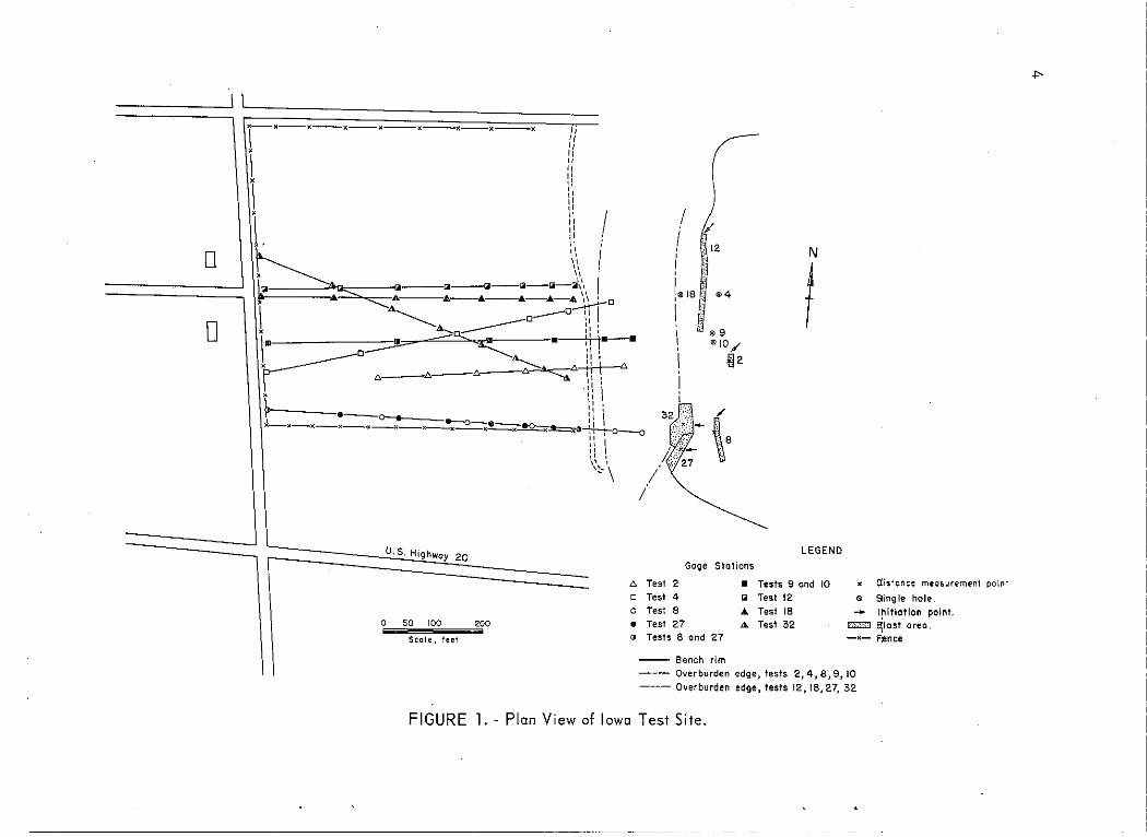
Figure l is a plan view of the Iowa test site showing the blast areas and gage locations. The gage array for each shot consisted of six to eight 3-component gage stations placed directly behind the blast area extending away from the blast. The gage array was moved frequently to keep it directly behind the blast area. Except for two tests the gage arrays remained approximately parallel to each other throughout the test program. Different symbols.have been used in figures 1 to 5 to show which gage stations were used to record a particular blast.

The blast areas and gage array of the Washington, D.C., site are shown in figure 2. The gage stations at this site were not moved at any time, but the gage boxes were removed after each blast and replanted for the next blast. Seven 3-component gage stations were used for all the blasts at this site.

0

0

X X l{ X X //

' " I, , ' , ::

l II I i: I .\ \\ .

" ' ' I: I l \\ :

r:ii-WI\\ I ~~ • --. --· --~0 \ a.. ll -- .. __ _.,_.. --o ,, I X -:S: A -- ~ ,,

r "' """'"~ ------a . :: :. --· I ~"'~ • -----:tt \1; 8 . ~ "'''' 'I• a -<> •----., :: : ~ -"" l:\ ' "' :: :

I I 12 N i

I ' l.,a ®4 ' I I •• ®[Q/

i ~2

I L

/ \1 I ' -e--o-o~ '' I ~~~--Q •-o-~----·- --·---- :l (1" , __ ,__ I~ \ -·-- --·-- \~~ \ \a

U.S. Highway 20

0 50 100 200

Scale, feet

"' a 0

• •

Gage Stations

Test 2 • Test 4 • Test 8 .. Test 27 " Tests 8 and 27

--Bench rim

LEGEND

Tests 9 and 10 Test 12 Test 18 Test 32

• -Distance measurement point

Slingle hole . l~itiation point.

~ ~lost area. -x- F~nce

--- Overburden edge, tests 2, 4, 8, 9, 10 ---- Overburden edge, tests 12, 18, 27, 32

FIGURE l,- Plan View of Iowa Test Site.

""'

"

\ I

l ;,; \ z ' \ ;;

\ I ~ ;;; £

"' : I N

¥ Test so/

)~t~ )T,, 54 I <

! I I l

0

0 3

50 100

0

4

N

~

Scale, feel

D Street NW

200

0

5

LEGEND

0

6

o Gage stations Distance measurement point

Initiation point

Presplil shol ~Blast area

---- Overburden edge

-~- Fence

FIGURE 2.- Plan View of Washington, D.C., Test Site.

6 5 4

QUARRY

\ 0 200 400 600

Scale, feet

LEGEND

Gage stoHons for tests 55 and 56 Gnqe stations for test 63

lJ. Gage stations for tests 64 and 65 o Gage stations for test 67

Distance meos~rement point ~Blast area -Bench rim I"""T"""r1 Quarry rim

---- 0\lerburden edge

- Initiation point

FIGURE 3.- Plan View of New York Test Site.

0

7

5

6

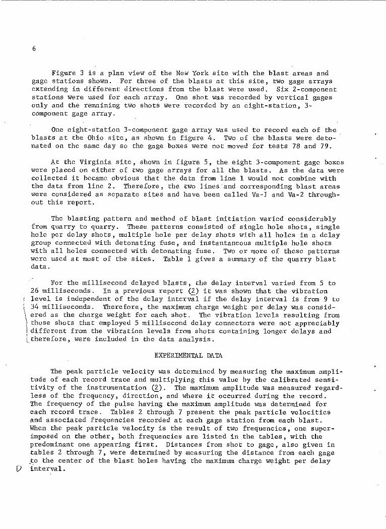
Figure 3 is a plan view of the New York site with the blast areas and gage stations shown. For three of the blasts at this site, two gage arrays extending in different directions from the blast were used. Six 2-component stations were used for each array. One shot was recorded by vertical gages only and the remaining two shots were recorded by an eight-station, 3-component gage array.

One eight-station 3-component gage array was used to record each of the blasts at the Ohio site, as shown in figure 4. Two of the blasts were deto­nated on the same day so the gage boxes 1>1ere not moved for tests 78 and 79.

At the Virginia site, shown in figure 5, the eight 3-component gage boxes were placed on either of two gage arrays for all the blasts. As the data were collected it became obvious that the data from line 1 would not combine with the data from line 2. Therefore, the two lines and corresponding blast areas were considered as separate sites and have been called Va-l and Va-2 through­out this report.

The blasting pattern and method of blast initiation varied considerably from quarry to quarry. These patterns consisted of single hole shots, single hole per delay shots, multiple hole per delay shots with all holes in a delay group connected with detonating fuse, and instantaneous multiple hole shots with all holes connected with detonating fuse. Two or more of these patterns were used at most of the sites. Table 1 gives a summary of the quarry blast data.

For the millisecond delayed blasts, the delay interval varied from 5 to 26 milliseconds. In a previous report (~) it was shown that the vibration

' level is independent of the delay interval if the delay interval is from 9 to \ 34 milliseconds. Therefore, the maximum charge weight per delay was consid­\ ered as the charge weight for each shot. The vibration levels resulting from ) those shots that employed 5 millisecond delay connectors were not appreciably ) different from the vibration levels from shots containing longer delays and L_therefore, were included in the data analysis.

EXPERIMENTAL DATA

The peak particle velocity was determined by measuring the maximum ampli­tude of each record trace and multiplying this value by the calibrated sensi­tivity of the instrumentation (~). The maximum amplitude was measured regard­less of the frequency, direction, and where it occurred during the record. The frequency of the pulse having the maximum amplitude was determined for each record trace. Tables 2 through 7 present the peak particle velocities and associated frequencies recorded at each gage station from each blast. When the peak particle velocity is the result of two frequencies, one super­imposed on the other, both frequencies are listed in the tables, with the predominant one appearing first. Distances from shot to gage, also given in tables 2 through 7, were determined by measuring the distance from each gage _to the center of the blast holes having the maximum charge weight per delay

D interval.

---

QUARRY

z----+---

CULi\\IATED FIELD

• 0

LEGEND

Goq:e stolion'l, te'i>\ 75 Gage stations, tests 78-79

Bench rim overburden edge

f"'T"T"'I Quarry rim Oistonce measurement point

c::=J B\OSI oreo tence line

b • 6 7

0 50 100 2.00

sc:ote' feel

400

~ \!'lilio\\On poinl

-¥~ Sil'lgle hole FIGURE 4-- Plan View of Ohio 1est Site.

7 6

0 50 100 2.00 400

Scole, feet

~ 0

" 7; 0 0 u •

QUARR'l'

LEGEND

P Gnge s.IQ.t\on'>, ((ne I t:. Goqe stations, Hoe 2

0'1stonce measurement point \n\liotion poinl Pfinwcmd Bench tim Overburden edge

~ Quot~'jlim ~ Btost area

FIGURE 5. ·Plan View of Virginia 1est Site.

7

8

TABLE 1._ - Quarry blast data

Test Total Hole Face Total Max. charge Charge No. of Length Burden, Spacing,

Site no. no. of depth, hgt.' charge, per delay, per hole, delay of delay, feet _ feet

holes feet feet pounds oounds -nounds intervals millisec

2 3 36 30 600 600 200 0 'o 10 15

4 1 36 30 200 200 200 0 0 10 -8 7 36 30 1,400 1,400 200 0 0 10 15

9 1 % 3{) ~88- 2:80 2-QO- Q Q 10 -Iowa ..•• ,. 10 1 36 30 200 200 200 0 0 10 -

12 15 36 30 3,000 3,000 200 0 0 10 15

18 1 36 30 200 200 200 0 0 10 -27 13 36 30 2,600 800 200 3 17 10 15 32 21 36 30 4,263 1,218 203 3 17 10 14

45 3 20 20 110 37 37 2 25(cap) 4 6

46 13 20 20 403 31 31 12 25(cap)_ 4 6.5

D.C •••••• 50 9 20 - 70 70 7.8 0 0 - 2.5

51 13 20 20 403 31 31 12 25 (cap) 4 6

52 13 20 20 325 25 25 12 25(cap) 4 6

54 13 18 20 308 25 24 avg 12 25(cap) 4 6

55 35 - 28- 54 21,578 920 920 34 17,26 22 20

56 13 - 83-104 18,471 1,522 1,100-1,522 12 26 22 20

63E 18 - 67- 73 19,933 1,249 1,039-1,249 17 26. 23 20

63SE - - - - - - - - - -

New York. 64N 6 - - 1,200 200 200 5 26 10-15 20 64E - - - - - - - - - -

65N 28 55-60 50- 55 28,810 1,405 700-],.,405 27 26 21 20

65E - - - - - - - - - -67 12 76-82 70- 76 ,14,576 1,355 1,100-1,355 11 26 22 22

Ohio ..... ) 75 36 24 23 6,430 1,072 180 9 9 12 10 78 36 56 54 16,520 4,620 459 12 9 14 11 79 1 56 54 468 468 468 0 0 10 -

96 84 20 18 3,350 1,120 40 avg 2 5 8 5

99 49 20 18 1,950 968 40 avg 1 5 8 5 101 78 20 18 3,200 1,600 40 avg 1 5 8 5 103 59 20 18 2,150 589 35 avg 3 5 8 5

Va .-1 .. ,. 104 60 15-20 15- 20 2,425 1,330 40 avg 1 9 8 6 106 61 20 18 2,350 1,380 40 avg 1 9 8 5 108 60 20 18 1,950 1,600 20-35 1 5 10 6

r09 51 20 12- 14 1,700 865 33 avg 1 5 8 5-7

110 51 20 18 1,750 360 32 avg 4 5 8 6 111 48 20 18 1,600 367 33 avg 4 5 8 6

98 31 20 18 1,250 605 40,3 avg 1 5 8 5 100 16 22-12 20- 10 475 475 25-35 0 0 8 5

Va.-2 .... 102 16 10-20 8- 18 450 343 25-35 1 5 8 5 105 42 4-20 4- 20 1,325 1,325 25-35 0 0 10 5 107 42 6-20 6- 20 1,250 1,250 25-35 0 0 8 5

" d e on e The length of the delay 1S considered to be zero 1f the shot cons1ste of a s1ngle hal , of e hal p er

delay, or of multiple holes per delay tied together with detonating fuse,

9

TABLE 2. - Particle velocity and frequency data for the Iowa site

Scaled Radial Vertical Transverse Test Distance, dis tanl'e, Particle Fre- Particle Fre- Particle Fre-

100 ft ft/lb'2 velocity, quency, velocity, quency, velocity, quency, in/sec cps in/sec cps in/sec CPS

2.13 8.69 - - 1. 74 50 .0. 789 50 3.13 12.8 1.47 25 1.17 25 .699 50

2 .. 4.13 16.9 .923 20 .680 40 .384 30 5.13 20.9 .680 16 .363 100 .199 25 6.13 25.0 .694 20 .324 40 .201 20 7.13 29.1 .511 16 .241 50 .228 16

2.20 15.6 1.45 24 1.08 167 .456 36 3.10 22.0 .597 26 .418 - .192 42

4 .. 3.89 27.6 .403 29 .280 200 .185 14 5.38 38.2 .325 21 .144 125 - -7.38 52.3 .150 21 .0898 133 .068 71 9.32 66.1 .0792 56 .0502 66 .044 20

1.45 3.88 - - 8. 76 15 1.65 25 2.00 5.35 6.92 15 5.45 14 .900 50 2.74 7.33 4. 65 14 2.27 50 . 932 20

8 .. 3.70 9.89 l. 94 50 2.11 50 .859 30 5.00 13.4 2.00 50 1.20 50 .614 50 6.75 18.0 1.45 50 .780 30 .381 50 9.07 24.3 .694 28 .350 20 .344 18

1.62 11.5 1.88 37 1. 79 71 .450 17 2.20 15.6 1.10 31 . 977 83 .245 83

9 .. 3.22 22.8 .475 42 .448 71 .269 71 4.55 32.3 .340 30 .238 125 .182 20 • 6.42 45.5 .169 36 .157 125 .103 20 9.03 64.0 .0811 23 .0710 83 .0589 31

1.62 11.5 2.34 50 1.64 71 .757 50 2.20 15.6 1.30 38 .892 111 .450 36

10 .. 3.22 22.8 .567 31 .448 71 .223 56 4.55 32.3 .386 30 .219 31 .182 26 6.42 45.5 .195 45 .137 105 .101 22 9.03 64.0 .0957 21 .0676 83 .0500 25

2.60 4. 75 - - 4. 72 25 2.41 25 3.06 5.58 5.10 16 2. 73 25 1.57 20 3.64 6.64 4.15 12 2.00 25 1.24 25

12 .. 4.36 7.96 3. 77 20 2.64 25 1.01 30 5.18 9.45 3.64 20 1.65 29 1.47 25 6.18 11.3 2.19 22 .866 25 1.09 22 7.36 13.4 1.49 20 .548 20 1.25 25 8.88 16.2 .903 15 .420 30 - -

10

TABLE 2. -Particle velocity and frequency data for the Iowa site--(Con.)

Scaled Radial Vertical Transverse Test Distance, distance, Particle Fre- Particle Fre- Particle Fre-

100 ft ft/1b~ velocity, quency, velocity, quency, velocity, quency, in/sec cps in/sec cps in/sec cps

2.20 15.6 1.66 22 0.998 25 0. 778 33 2.67 18.9 .713 13 .850 83 .696 26 3.24 23.0 . 780 18 .347 38 .621 26

18 .. 4.10 29.1 . 634 19 .342 32 .279 18 4.76 33.8 .630 27 .205 28+114 .355 18

. 5.79 41.1 .266 24 .105 23+143 .239 20 7.04 49.9 .215 18 .126 22 .243 18 8.53 60.5 .131 14 .0965 27 .146 15

2.14 7.56 4.48 12+125 - - 1.13 10+50 2.63 9.29 1.08 100 2.39 125 3.08 100 3.21 11.3 1.80 12+75 1.38 50 .859 12+83

27 .. 3.90 13.8 1.91 25 1.25 133 1.06 12 4. 75 16.8 1.52 26 .744 28+100 .788 17 5.75 20.3 1.54 29 .786 25+100 - -6.95 24.6 .729 12 .504 25+100 .345 12 8.40 29.7 .387 18 .228 10 .237 7.5

2.55 7.31 4.32 8.5 1.33 85 1.15 11+100 3.05 8.74 1.80 14 - - .835 52 3.65 10.5 1.58 20+86 1.15 80 1.15 15

32 .. 4.40 12.6 1. 79 16+80 1.37 10+86 .849 14+60 5.30 15.2 1.28 16 .742 35 .988 18 6.35 18.2 1.02 19 .522 40+75 .448 19+100 7. 65 21.9 1.04 17+72 .406 75 .438 115 9.24 26.5 .533 18+75 .328 76 .164 20

11

~BLE 3. - Particle velocity and frequency data for the D.C. site

Scaled Radial Vertical Transverse Test Distance, distance, Particle Fre- Particle Fre- Particle Fre-

ft ft/lbl;, velocity, quency, velocity, quency, velocity, quency, in/sec cps in/sec cps in/sec cps

160 26.3 0.625 91 0.909 71 0.659 83 290 47.7 .415 67 .404 35 .281 77

45 .. 546 89.8 .118 27 .133 100 .274 83 705 116 .114 40 .0857 59 .0940 111 882 145 .0531 40 .0690 83 .0339 so

154 27.6 .426 71 .517 63 .398 63 207 37.2 .297 77 .347 77 .249 71 283 50.8 .290 63 .207 36 .140 71

46 .. 393 70.6 .148 45 .114 100 .0834 112 537 96.4 .110 56 .0685 63 .0857 so 697 125 .0935 48 .0425 71 .0583 63 875 157 .0294 56 .0396 63 .0301 45

)"' 21.0 1.27 59 1.04 59 .389 43 286 34.2 .405 43 .465 42 .184 143

50 .. 430 51.4 .264 36 .261 35 .159 33 590 70.5 .155 30 .116 42 .137 36 765 91.4 .0689 30 .0785 30 .0471 37

155 27.8 .344 67 .373 31 .291 43 209 37.5 .348 63 .417 40 .278 50 286 51.3 .373 43 .258 59 .170 100

51 .. 396 71.1 .186 38 .136 134 .0966 25+140 540 96.9 .128 36 .0804 36 .0761 31 700 126 .101 40 .0517 71 .0613 56 877 157 .0366 59 .0417 67 .0335 27

175 34.3 .186 111 .418 29 .189 36 229 44.9 .212 71 .242 35 .179 33 306 60.0 - - .156 45 .0995 45

52 .. 416 81.6 .0878 40 .0803 130 .0658 29 560 110 .0581 33 .0726 28 .0649 27 720 141 .0477 32 .0380 29 .0477 45 897 176 .0253 33 .0335 37 .0219 24

176 35.2 .446 100 .471 71 .212 71 250 50.0 .466 63 .334 67 .271 28

54 .. 359 71.8 .183 33 .210 37 .128 23+143 502 100 .126 27 .128 91 .0739 40 661 132 .0814 26 .0745 33 .0839 45 837 167 .0560 29 .0489 63 .0309 36

12

~BLE 4. - Particle velocity and frequency data for the New York site

Scaled Radial Vertical Transverse Tes Distance, distanc~, Particle Fre- Particle Fre- Particle Fre-

100 ft ft/lb" velocity, quency, velocity, quency, velocity, quency, in/sec cps in/sec cps in/sec cps

4.68 15.5 - - 0.737 28 - -5.68 1<>.8 - - .4715 40 - -

55 .. 6. 70 22.1 - - .263 50 - -8.05 26.6 - - .245 40 - -

11.4 37.7 - - .164 36 - -17.1 56.5 - - .203 38 - -

10.7 27.4 - - .347 49 - -19.3 49.4 0.174 12.5 .0775 20 0.148 11 20.3 51.9 .0716 64 .0560 40+100 .101 40 21.3 54.6 .0537 51 .0457 63 .101 60

56 .. 22.7 58.2 .0768 40 .0746 80 .0891 9+60 24.3 62.2 .0582 50 .0631 100 .0699 63 26.3 67.3 .0571 50 .0499 45 .0953 50 28.5 73.1 .0439 40 .0464 42 .0567 8.5+33 31.7 81.3 .0909 40 .0861 40 .0862 49

3.00 8.50 1.24 29 1.34 25 - -4.25 12.0 1.16 43 1.46 17 - -

63E. 6.00 17.0 .880 23+50 .835 18 - -

8.50 24.1 .588 25 .620 12.5 - -12.0 34.0 .281 10 .344 12 - -17.0 48.2 .194 14 - - - -

3.00 8.50 1.24 29 1.34 25 - -5.70 16.1 .549 38 .581 9 - -

63SE 7.70 21.8 .732 16+51 .618 13+22 - -10.9 30.9 .228 22 .207 33 - -13.5 38.4 .166 50 .245 38 - -

3.00 21.3 .627 26+110 .438 25+133 - -4.00 28.4 .397 20 .303 32+77 - -

64N. 6.50 46.1 .101 17+100 .137 25+100 - -7.80 55.3 .156 17 .0818 29+100 - -

10.9 77.3 .106 15+74 .0520 22 - -15.0 106 .0322 11+83 .0357 16 - -

3.90 27.7 .17 29 .13 25 - -5.00 35.5 - - .052 17 - -

64E. 6. 90 48.9 .0854 25 .051 23+50 - -8.50 60.3 .114 18 .0737 25 - -

11.8 83.7 .033 12.5 .035 10 - -14.4 102 .019 12 .018 12 - -

3.00 8.00 0.657 39 .705 42 - -4.00 10.7 .658 17 .634 42 - -

65N. 6.49 17.3 .258 22 .202 18 - -7.80 20.8 .258 18 .121 23+71 - -

10.9 29.1 .220 8.5+40 .124 20 - -15.0 40.0 .177 10 I .0676 8.5 - -

13

TABLE 4. - Particle velocity and frequency data for the New York site--(Con.)

Scaled Radial Vertical Transverse Test Distance, distanct:, Particle Fre- Particle Fre- Particle Fre-

100 ft ft/lb" velocity, quency, velocity, quency, velocity, quency, in/sec cps in/sec cps in/sec cps

3.00 8.00 2.08 25 1.80 38 - -6.00 16.0 . 966 43 . 760 42 - -

6SE. 7.65 20.4 .718 13+26 .358 83 - -10.9 29.1 .207 12+43 .125 9+33 - -13.6 36.3 .133 12+57 .lOS 10+31 - -

2. 95 8.02 1.49 33 1. 63 37 1.46 56 3.55 9.65 1.86 10 1.33 43 1.16 25 4.40 12.0 .977 10 .676 so .560 12.5

67 .. 5.40 14.7 .456 7.2 .518 20+67 .517 77 6.75 18.3 .387 18 .311 45 .388 83 8.35 22.7 .311 so .211 so .269 12.5

10.3 28.0 .146 9+59 .158 50 .141 63 12.8 34.8 - - .128 so .124 so

TABLE 5 - Particle velocity and frequency data for the Ohio site

Scaled Radial Vertical Transverse Test Distance, distance, Particle Fre-. Partlcle Fre- Particle Fre-

100 ft ft/lblz velocity, quency, velocity, quency, velocity, quency, in/sec CDS in/sec cps in/sec cps

2.32 7.09 2.17 26 1. 79 59 2.19 so 2. 93 8.96 2.31J 29 1.49 so 1.41 36 3.74 11.4 2.19 42 1.14 56 1. 68 so

75 .. 4.82 14.7 . 909 66 1.31 45 .967 29 6.30 19.3 .764 36 .896 75 .560 36 8.10 24.8 . 791+ 28 .950 83 1.02 71

10.7 32.7 .407 30+100 .401 42 .418 28 14.0 42.8 .309 16 .0867 12 .348 15

4.60 6.76 2.06 19 2.85 22 2.32 11 5.41 7.96 2.19 28 1.86 26 1. 67 28 6.40 9.41 2.01 25 1.31 33 1.18 15

78 .. 7.82 11.5 1.72 19 .912 27 .861 12 9.62 14.1 1.47 25 .786 50 .834 25

11.9 17.5 1.09 so .674 42 .788 15 15.0 22.0 .590 13 .373 29 .936 13 18.9 27.9 .307 25 .278 16 .263 22

4.96 23.0 0.401 36 0.611 31 0.395 18 5.78 26.8 .384 31 .278 28 .334 24 6.76 31.3 .341 29 .134 42 .251 22

79 .. 8.19 37.9 .287 28 .147 33 .246 22 9. 98 46.2 .235 24 .101 42 . 261 25

12.3 56.8 .152 22 .0806 36 .182 20 15.3 71.1 .120 18 .0546 28 .156 20 19.3 89.4 .0669 25 .0422 17 .0474 25

14

Test

96

99

101

103

104

TABLE 6. - Particle velocity and frequency data for the Virginia site line 1

Scaled Radial Vertical Transverse Distance, distance, Particle Fre- Particle Fre- Particle Fre-

lQ() .1'!: ft 11!>11 V§loci,!:y, 'll!§!"l<:!Y, V§lg<::it;y, __ qlJ?PoGY ,_ V('lQ!::i!;y, _q!!~r!GY, in/sec CDS in/sec cps in/sec cps

4.12 12.3. 0. 962 38 - - 0.886 27 4. 75 14.2 1.39 23 1.54 31 1.62 26 5.60 16.7 1.03 19 .683 34 - -6.88 20.5 - - .423 35 .900 24 8.45 25.2 .772 14 .334 23 .378 24

10.40 31.0 .383 11 .314 17 .301 12.5 13.10 39.1 .471 25 .159 100 .285 39

3. 95 12.7 1.85 33 1.67 38 1.92 22 4.56 14.7 1.20 36 1.33 36 1.42 25 5.42 17.4 0.861 25+100 . 628 63 1.53 25 6.67 21.4 - - .824 38 .845 29 8.24 26.5 .692 21 .406 36 .472 38

10.20 32.8 .328 20 .342 18 .328 18 12.90 41.5 .334 25 .215 36+100 .313 25

3.88 9.70 1.64 68 l. 81 28 l. 90 22 4.52 11.3 1.09 25 1.14 31 1.57 23 5.42 13.5 1.17 25+75 1.02 50 2.25 28 6.70 16.7 - - .714 31 .764 25+50 8.29 20.7 .946 17 .461 26 .616 22

10.30 25.7 .938 16 .340 20 .434 16 13.00 32.5 .358 25+63 .198 83 .347 77

! 3.56 14.6 .840 80+17 1.09 38 1.25 26 4.18 17.2 .773 60 .580 67 1.09 22 5.02 20.7 .602 71 .500 87 1.01 25 6.29 25.9 - - .243 100+20 .474 24 7.85 32.3 .346 21 .318 24 .493 25

( 9.83 40.5 .223 14 .249 18 .232 17 12.50 51.4 .195 28 .0929 71 .353 24

3.10 8.49 - - 1.24 26 - -3.76 10.3 0.558 57 1.04 24 1.89 30 4.64 12.7 .786 25 .863 50 1.38 29 5. 93 16.2 - - .456 30 1.10 35 7.51 20.6 .634 18 .434 26 .860 36 9.50 26.0 .296 13 .285 22 .276 19

12.25 33.6 .384 23 .129 56 .535 28

Test

106

108

109

llO

111

TABLE 6. - Particle velocity and frequency data for the Virginia site line 1--Continued

15

Scaled Radial Vertical Transverse Distance, distance, Particle Fre- Particle Fre- Particle Fre-

1 100 ft ft/lb" velocity, quency, velocity, quency, velocity, quency, in/sec ·Cps in/sec cps in/sec cps

2.86 7. 71 2.08 38 1.40 21 - -3.50 9.43 1.98 26 1.42 26 2.00 21 4.38 ll.8 .922 36 1.09 38 1.61 25 5.65 15.2 - - .600 36 1.58 31 7.24 19.5 .566 29 .529 26 1.18 36 9.21 24.8 .435 10 .384 23 .348 21

12.00 32.2 .323 23 .161 40 .363 22

2.50 6.68 1.42 31 1.43 29 2.17 26 3.15 8.42 1.52 24 2.01 33 1.44 28 4.00 10.7 1.13 29 . 959 29 1.41 40 5.32 14.2 - - .727 33 . 657 31 6.02 16.0 1. 02 22 . 977 26 1. 70 24 6.90 18.4 • 7ll 22 .448 31 .628 33 8.87 23.8 .387 12 .263 17 .338 17

11.60 31.0 .270 23 .124 31 .392 22

2.14 7.28 2.19 42 1.55 45 1.26 17 2.78 9.46 1.09 25 1.12 27 1.85 29 3.62 12.3 .736 67 .766 31 1.29 27 4.88 16.6 - - .373 56 .597 33 5.55 18.9 .863 31 .800 22 .958 31 6.43 21.9 .387 25 .334 25 .628 36 8.44 28.7 .223 45 .264 25 .240 17

11.20 38.1 .273 26 .105 50 .286 25

2.13 11.2 1.10 31 1.06 42 1.14 33 2.78 14.6 .420 23 .472 48 1.09 30 3.68 19.4 - - - - .675 27 4.97 26.2 .680 29 - - - -5.67 29.8 .484 33 .283 22 .345 34 6.56 34.5 .245 10 .144 25 .235 43 8.52 44.8 .181 14 .0847 17 .112 63

ll.3 59.4 .124 67 .120 100 .142 21

2.00 10.2 1.12 38 1.01 43 1.45 31 2.64 13.5 .465 31 . 712 71 1.23 33 3.50 17.9 .539 35 .581 53 .627 71 4.80 24.5 .871 30 .518 48 .420 31 5.50 28.0 .570 34 .278 21 .285 34 6.40 32.6 .290 ll .211 26 .328 40 8.38 42.7 .155 9 .0884 13 .143 40

11.1 56.6 .280 24 .121 42 .195 24

---------------- ------

16

TABLE 7. -Particle velocity and frequency data for the Virginia site line 2

Scaled Radial Vertical Transverse Test Distance, distance, Particle Fre- Particle Fre- Particle Fre-

100 ft ft/lb~ velocity, quency, velocity, quency, velocity, quency, irL/B£<:. ~<OJlR in/s= CPB ~in/~~ <;;pl>

3.94 16.0 1.61 38 1. 76 54 1.67 42 4.78 19.4 0.679 36 .788 36 .794 40 5.69 23.1 .829 36 .917 83 1.28 28

98 6. 72 27.3 .550 75 .346 85 .692 23 8.13 33.0 .517 36 .233 83 .592 28 9.70 39.4 .381 15 .142 20 .338 15

11.80 48.0 .106 11+75 .0929 93 .119 77 13.90 56.5 .lOS 28+100 .0991 100 .0788 100

5.52 25.3 1.06 33 .693 37 .611 33 6.36 29.2 .328 50 .267 42 .380 33 7.27 33.3 .573 24 .173 33 .328 37

100 8.31 38.1 .442 23 .230 23 .409 28 9.71 44.5 .333 25 .121 25 .293 23

11.30 51.8 .258 66 .178 20 .204 25 15.50 71.1 .0640 24 .0484 20+110 - -

4. 77 25.8 .672 37 .281 so .280 35 5.61 30.3 .246 45 .185 56 .211 45 6.51 35.2 .430 31 .136 63 .469 36

102 7.57 40.9 .196 30 .113 36 .261 27 8.96 48.4 .173 32 .0579 42 .153 28

10.50 56.8 .110 23 .0484 22+56 .0681 43 \ 14.70 79.5 .0306 42 .0285 50 .0299 39

I'·" 22.7 . 995 29 1.15 33 .536 29 10.00 27.5 .873 26 - - .497 26

105 11.00 30.3 .581 83 .424 22+250 .421 22 12.40 34.1 .598 22 .283 19 .464 26 14.00 38.5 .310 12 .217 17 .240 19

9.47 26.8 .483 28 .670 30 .552 29 10.30 29.0 .253 55 .278 46 .248 38 11.20 31.6 .549 26 .216 71 .403 33

107 12.20 34.5 .323 . 22 .257 25 .341 25 12.80 36.1 .435 31 .173 27 .280 25 13.60 38.4 .347 25 .366 22 .235 19 15.20 42.9 .161 12 .130 19 .140 16 17.30 48.9 .171 50 .0571 17+120 - -

DATA ANALYSIS

For each test, the peak particle velocity recorded at each gage position was plotted by component on log-log coordinates as a function of distance from

17

the blast area. Good linear grouping of the data was obtained, indicating that the particle velocity-distance data for each set of data can be represented by a straight line. The method of least squares was used to obtain a measure of the spread in the data, and to determine the slope and intercept of the best fit straight line through each set of data (~).

The straight lines are shown plotted through the midpoints of the data in figures 6 to 8. Because of the large amount of data, it is not possible to show each data point. The standard deviation of the data about each straight line is shown as a vertical line near the center of the data. The straight lines in figures 6 to 8 can be represented by a general propagation equation of the form

v

where v = peak particle velocity,

D = travel distance,

[llj = exponent of D or the slope of the straight line through the jth set of data at the ith site,

and Ku = velocity intercept at unit travel distance for the jth set of data at the ith site.

The letter i represents the site, and varies from 1 to 6, whereas the letter j represents a test at each site, and varies from 1 to k

1 where k

1 is the total

number of tests at any given site.

As written, equation 4 indicates that for each component the slope, ~!j, varies with each shot at each site. However, it is apparent from figures 6 to 8 that the slopes, s,j' may not vary significantly from shot to shot for a given component at each site. Therefore, analysis of variance tests were per­formed on the data to determine if significant differences in s,j exist for a given compnent at each site. A summary of these tests is given in table 8.

-J( The calculated F1 values are all larger than the table values; thus, there are significant differences between the sets of data and one straight line can not represent all the test data for each component at each site. Because the cal­culated values of F2 are all smaller than the F2 table values, there are no significant differences in the slopes for the different tests at each site for each component. Thus, an average slope, ~ 1 , can be used for each component at each site. These average slopes are given in table 8.

To determine if significant differences in slope exist because of site effect, the data from all sites were grouped together by component, and an analysis of variance test performed. The results are summarized on the last line for each component in table 8, and show that there is a significant dif­ference in slope with site for two of the components. No attempt was made to combine the data by component, or to use an average slope at all sites for the transverse component.

a-1../), t-i-;£t: c:t·', t. t .· ·/ l(f/L<--~ L_,! __ !il.-r .. r.' .9 A-.'( i .:) -t-~.tQ

M.t J;" C ND .1

--·--------- ----

18

-c c 8 .. "' ~ .. 0.

"' Q) .s:::: u <:

>-1--u 0 ....J w > w ....J u 1-­oc rt ~ <( w n.

8. 0 r------.---r---.---,--,

6.0

4.0

2.0

1.0 .8 .6

.4

.2

.I

/!,

D 4 0. 8

" 9 • 10 • 12 ... 18 ? 27

" 32

4. 0 ,----.-----.----r--r•

2.0

1.0 .8 ,6

.4

.2

.I .08 .06

.04

D.C.

Symbol ... 45 D 46 /!,. 50 0 51 • 52 • 54

.0 2 '---'---.l..-_L...L....l

I 2 4 6 8 10 2

Symbol Tesl

D 75

OHIO

/!, 78 . 0 79

N.Y.

4 6 8 10

VA. I

""~.h~' Tesl

0 96 0 99 • 101 /!,. 103 • 1"04 ... 106

"' 108 109

1-S••mb,nl Tesl

Symbol Tesl

0 56

\

~ 63E <il 63SE o 64N • 64E [> 65N <l 65E • 67

20 40 2

" 110 a II I

Symbol Tesl

0 98 D 100 • 102 /!, 105 " 107

VA.2

4 6 8 10

Dl STANCE, hundreds of feet

FIGURE 6.- Peak Particle Velocity Versus Distance, Radial Component.

20

19

10.0 8.0 Symbol Test

6.0 IOWA OHIO VA. I 0 96 0 99

4.0 • 101 {; 103

• 104

2.0 • 106

"' 108

" 109

1.0 110

.8 Ill

.6 ...,

.4 <= Symbol 0 u "' {; 2 "' ~ .2 0 4 "' 0 8 c.

"' " 9 Symbol Test Q) • 10 .r::: .I 12 0 75 u • <= .08 18

{; 78 • 79 0

>- .06 "' 27 1-- "' 32 u .04 9 3.0 w > Symbol Test w 2.0

D.C . N.Y. {; 55 VA. 2. ...J u 0 56

1-- .. 63E a-: 1.0 .. 63SE <( .8 0 64N Q_

. 6 • 64E

"' I> 65N <( w .4 <I 65E Q_ • 67

.2

. I .08 .06 Symbol Test

• 45 Symbol Test . 04 0 46 0 98

{; 50 0 100 0 51 • 102

.02 • 52 {; 105

• 54 • 107

. OJ 2 4 6 8\0 2 4 6 8 10 20 40 2 4 6 8 10 20

Dl STANCE, hundreds of feet

FIGURE 7.- Peak Particle Velocity Versus Distance, Vertical Component.

20

"0 c 0 u Q) V>

~

Q) a. V> Q)

.s:; u c

>-1-u g w > w _J u 1-a: if: ~ <( w (L

8 . 0 .-----.------,--,-----,-,

6.0

4.0

2.o··

1.0 .8 .6

.4

.2

. I .08 .06 .05

I

Symbol Test IOWA t;. 2 OHIO

0

0

" •

Symbol Test

• 12 ... 18 .,. 27 () 32

2 4 6

2.0

1.0 .8

.6

.4

.2

.I .08

.06

.04

8 10 2

D.C.

Symbol 0

t;.

0

4

Symbol ... 0 [j,

0

• •

Test

75 78 79

6 8 10

Test 45 46 50 51 52 54

.02L---~---L~~~

Symbol A 'I'

" ()

"' 20 2 4

I I

~,\' VA. 2

Symbol Test 0 98 0 100 • 102 t;. I 05 • 107

I 2 4 6 8 10 3 4 6 8 10

DISTANCE, hundreds of feet

Symbol Test

0 96 0 99 • 101 t;. 103 • 104

Test 106 108 109 110 Ill

6 810

~

20

FIGURE 8. · Peak Particle Velocity Ve·rsus Distance, Transverse Component.

20

21

~BLE 8. - Statistical tests for particle velocity versus distance data

F 2 F 3 Average 1 2 Component Site· ki nl Table4 Calcu- Table4 Calcu- 8,

lated lated

Iowa 9 60 1.89 36.91 2.17 1.53 -1.576 D.C. 6 36 2.26 5.57 2.62 1.04 -1.384

Radial .....••.••..• N.Y. 8 48 2.02 12.94 2.32 1. 91 -1.431 Ohio 3 24 2. 93 53.97 3.55 .22 -1.255 Va. l 10 62 1.86 7.88 2 .ll 1.12 -1.086 Va. 2 5 35 2.34 11.53 2.76 .36 -2.148

All 41 265 1.38 30.39 1.55 2.26 -Iowa 9 61 1.89 57.83 2.17 1. 71 -1.766 D.C. 6 37 2.24 20.35 2.60 1.24 -1.548

Vertical .....•..... N.Y. 9 56 1.92 20.50 2.19 1.97 -1.475 Ohio 3 24 2.93 25.56 3.55 .57 -1.497 Va. 1 10 71 1. 76 9.77 2.05 .40 -1.548 Va. 2 5 34 2.36 21.64 2.78 1.06 -2.346

All 42 283 1.38 30.67 1.55 1.69 -

Iowa 9 60 1.89 28.26 2.17 2.17 -1.189 D.C. 6 37 2.24 3.17 2.60 .24 -1.285

Transverse ......... N.Y. - - - - - - -Ohio 3 24 2. 93 23.03 3.55 .34 -1.083 Va. 1 10 70 1. 78 7.79 2.07 .49 -1.389 Va. 2 5 33 2.38 9.67 2.80 .89 -2.064

All 33 224 1.44 32.16 1.65 1.52 -1 Total number of data points. 2 A calculated value of F1 greater than the table value means that one line

cannot be used to represent all the data. 3 A calculated value of F2 less than the table value means that the slopes are

not significantly different. 4 Table values are for a 95 percent confidence interval.

(,·,,·' With the assumption that the straight line passes through the midpoint of

the data, the average slope, f:l 1 , for each component at each site was used to calculate the intercept, K1 , for each test. To reduce the variance in the intercepts, distances were Aetermined in units of 100 feet. Therefore, K1 J is the particle velocity at 100 feet. The values of ~j are summarized in table 9 along with the maximum charge weight per delay interval. It can be seen from this table and from the plots in figures 6 to 8 that the level of vibra­tion generally increases as charge weight per delay increases.

As a result of the statistical tests described above the general propaga­tion equation 4 for each component can now be written as

v (5)

22

where

and

v = particle velocity in in/sec,

D = distance in units of 100 ft,

K1 J velocity intercept at D = 1,

si = ave-r-age sl<>p" of the J set-s of data at the ith site when these data are plotted on log-log coordinates.

Equation 2 written in a generalized form to represent data from different sites, becomes:

v (6)

where D distance in units of 100 ft,

W1 J maximum charge weight per delay interval for each

and

test in units of 100 lbs,

the velocity intercept at D/Wa the ith site.

1 for all the tests at

Comparison of equation 5 with equation 6 shows that the following rela­tionship must exist:

a,~! K1 l = H1 W1 l (7)

Equation 7 implies that a log-log plot of the K1 J values against the charge weight per delay, W1 J, should result in a linear grouping of the data by site and component.

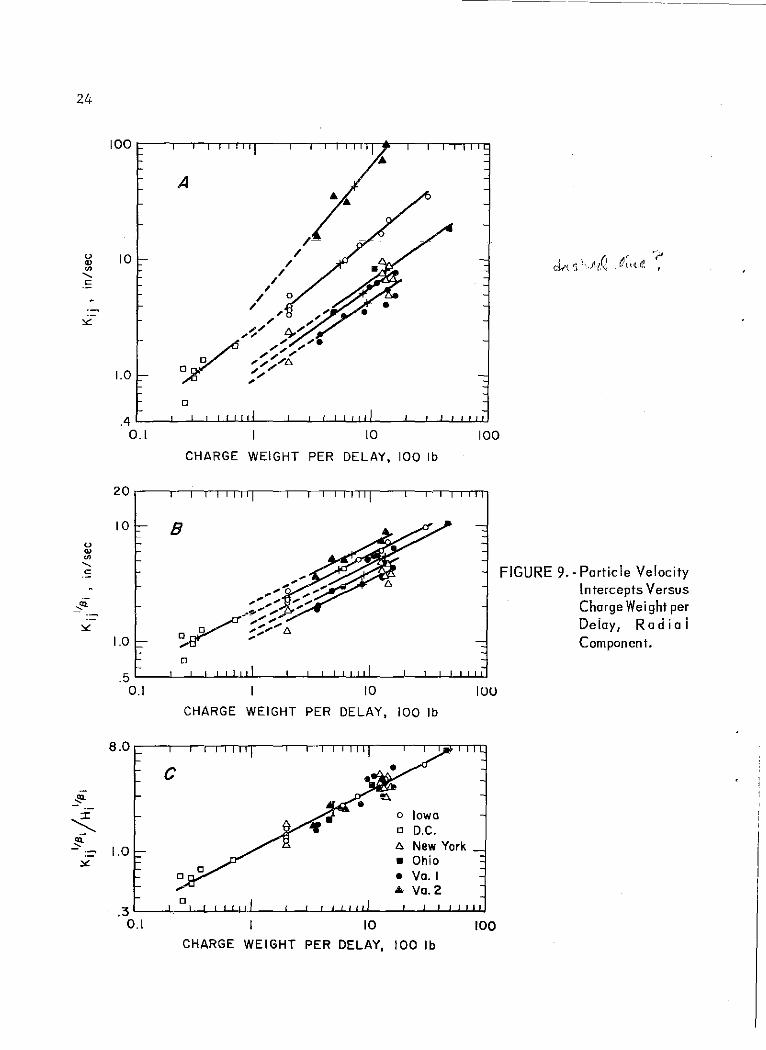
Log-log plots of K1 J vs W1 J (data given in table 9) were made and are shown in figures 9a, lOa, and lla. Examination of these plots shows that the data for each site are independently distributed about their own straight line, thus indicating that both the slope, as1 ~ and the intercept, H1 , are functions of site and component. The ~ethod of least squares was used to determine the slopes, aS1 , and intercepts, H1 ~ These values are given in table 9.

Equation 7 can be rewritten as:

(H ) 1/~, w. a i l J • (8)

Equation 8 is interpreted as follows: If wa is a scaling factor, then a plot

of (K1 J)l/~ 1 versus W1 J on log-log coordinates should result in the data grouping about a series of parallel straight lines having a slope of a. The average values of si for each site and component, given in table 8, were used to calculate the quantities (K1 J)l/~,. These values are shown plotted as a function of W1 J on log-log coordinates in figures 9b, lOb, and llb. The method of least sq-uares was used to determine the slOpes, a 1 , and their vari­ances, Sa , for the straight lines through the data from each site and com-

1

ponent are given in table 10.

23

TABLE 9. -Summary of K1 j, aS1 , and H1 data

Maximum Radial Vertical Transverse Site Test charge K! J> a.B! HI

per delay, in/sec ~ j' a~! HI

in/sec Ki J '

in/sec aS1 HI

lbs 2 600 9.88 0.830 2.24 7.61 0.753 2.13 1.99 0. 710 0.675 4 200 3. 72 - - 3.12 - - .817 - -8 1,400 22.1 - - 18.4 - - 3.35 - -9 200 3.34 - - 3. 77 - - .874 - -

Iowa 10 200 3. 95 - - 3.51 - - .992 - -12 3,000 35.2 - - 23.3 - - 7.94 - -18 200 4.88 - - 3.60 - - 2.07 - -27 800 13.3 - - 12.9 - - 4.27 - -32 1 ,218 16.9 - - 13.2 - - 4.19 - -

45 37 1.38 0. 774 2.52 1.92 0.741 2. 96 1.16 0.525 1.22 46 31 .947 - - .997 - - .603 - -

D.C. 50 70 1.81 - - 2.17 - - . 875 - -51 31 1.08 - - 1.10 - - .624 - -52 26 .586 - - .897 - - .461 - -54 25 1.15 - - 1.37 - - .637 - -

55 920 - 0.724 1.09 6.59 0.802 0.861 - - -56 1,522 6.73 - - 6.94 - - - - -63E 1,249 9.80 - - 11.4 - - - - -63SE - 7.64 - - 8.76 - - - - -

N.Y. 64N 200 2.39 - - 2.00 - - - - -64E - 1.31 - - 1.00 - - - - -65N 1,405 5.01 - - 3.60 - - - - -65E - 8.99 - - 6.81 - - - - -67 1,355 6.58 - - 6.04 - - - - -

) 75 1,072 8.40 0.709 1.32 10.1 0.784 1.25 5. 77 0.616 1.04

Ohio 78 4,620 18.8 - - 23.2 - - 10.1 - -79 468 3.53 - - 3.58 - - 2..29 - -

96 1,120 6.37 0.696 .906 10.4 0. 742 1.45 9.37 0.762 1.54 99 968 5.89 - - 12.1 - - 11.2 - -

101 1,600 7.58 - - 12.7 - - 13.1 - -103 589 3.23 - - 6.13 - - 7.90 - -

Va.l 104 1,330 4.06 - - 8.08 - - 11.9 - -106 1,380 5.46 - - 9.48 - - 12.6 - -108 1,600 4.91 - - 8. 71 - - 2.23 - -109 865 3.54 - - 5.89 - - 1. 90 - -110 360 1. 99 - - 3.18 - - 1.26 - -111 367 2.28 - - 3.75 - - 1.35 - -

98 605 31.8 1.21 4.04 36.3 1.49 2.30 29.2 1.05 3.82 100 475 34.7 - - 29.4 - - 24.6 - -

Va.2 102 343 15.7 - - 11.8 - - 11.0 - -105 1,325 106 - - 120 - - 58.1 - -107 1,250 71.7 - - 81.9 - - 48.8 - -

--------------

24

" 10 cJ,., '.; '·J'IQ ~~,,~ ..,

"' V>

' <=

, "' /

1.0 of D

A 0.1 10 100

CHARGE WEIGHT PER DELAY, 100 lb

20

10 8 " "' "' ' FIGURE 9. ·Particle Velocity <=

Intercepts Versus -,. "'- Charge Weight per

--Deiay, Ra d 1 a i "' 1.0 Component.

D

.5 0.1 10 100

CHARGE WEIGHT PER DELAY, 100 lb

8.0

c -,."'-

~ 0 Iowa IJ D.C.

J;-1.0 " New York -- Ohio "' •

• Va.l

" Va.2 IJ

.3-0.1 10 100

CHARGE WEIGHT PER DELAY, 100 lb

" Q)

"' ' <=

" Q)

"' '-<=

:::-"' ·-

""

~

~ ~-

·-"'

100

10

1.0 .8

0.1

CHARGE WEIGHT

20

10 B

1.0

.5 0.1

CHARGE WEIGHT

8.0

c

1.0

. 3 0.1

CHARGE WEIGHT

25

10 100

PER DELAY, 100 lb

FIGURE 10.- Particle Velocity

Intercepts Versus

Charge Weight per De lay, Vertical Component.

10 100

PER DELAY, 100 lb

o Iowa o D.C. {; New York • ·Ohio • Va. I ... Va.2

10 100 PER DELAY, 100 lb

16

u

'" '" .... "

u

'" '" ' c

I j I 'I 1 I I I I r lj

10

1.0

a .4L-~--~~~~--~~~-U~--~~~~~

0.1 10 100

CHARGE WEIGHT PER DELAY, 100 lb

10 ::- B -

-

- FIGURE 11.- Particle Velocity

1.0 -

c

1.0

0

0

10

o Iowa a D.C. "" New York • Ohio • Va. I A Va.2

CHARGE WEIGHT PER DELAY, 100 lb

-

100

100

Intercepts Versus Charge Weight per Delay, Trans­verse Component.

27

~BLE 10. - Statistical test for (K1JJl/S, versus W1 J

F 1 F 2

Component Site Slope sa, No. of l:ki Table"' Calcu- Table" Calcu-a, sit~s lated lated

Iowa 0.527 0.026 6 41 2.18 7.64 2.54 0.26 D.C. .558 .229 - - - - - -

Radial. •..• N.Y. .506 .089 - - - - - -Ohio .568 .105 - - - - - -Va. 1 .637 .118 - - - - - -Va. 2 .567 .090 - - - - - -

Iowa .427 .028 6 42 2.16 5.04 2.53 .54 D.C. .474 .197 - - - - - -

Vertical .•• N.Y. .546 .119 - - - - - -Ohio .523 .113 - - - - - -Va. 1 .479 .089 - - - - - -Va. 2 .63 7 .078 - - - - - -

Iowa .598 .097 5 33 2.38 7.59 2.80 .16 D.C. .412 .267 - - - - - -

Transverse. Ohio .566 .176 - - - - - -Va. 1 .550 .087 - - - - - -Va. 2 .516 .085 - - - - - -

1 A calculated value of F1 greater than the table value means that one line cannot be used to represent all the data.

2 A calculated value of Fa less than the table value means that the slopes are not significantly different.

3 Table values of F1 and F2 are for a 95 percent confidence interval.

l/S 1 An analysis of variance test was perfopmed on the (K1 J) vs(W1 J) data from all sites, grouped by component to determine if one line could be used to represent all the data by component or if a series of parallel lines could be used to represent the data from each site. These analysis of vari­ance tests are summarized in table 10, and the results show that one line cannot represent all the data for each component, but that an average slope for each component can be used for all sites. These average slopes, a, and their variances, Sa, were computed and are given in table 11. Statistical t tests were performed to determine if the average slopes differ significantly from a theoretical value of 0.5. The results of these t tests, summarized in table 11, show that there is no significant difference between each of the average slopes and the theoretical value of 0.5. Therefore, the theoretical

? slope of 0.5 was placed through the data as shown in figures 9b, lOb, and llb. Examination of these figures shows that the value of (K)l/S, at a particular charge weight is a function of the quarry site.

28

TABLE 11. - Statistical tests for comparison of slope a with theoretical value of 1/2

Component Degrees Average Sa Theoretical of freedom slope a value Table2

Radial .......... 34 0.545 il. 034 0.500 2.03 Vertical .....•.. 35 .491 .037 .500 2.03 Transverse ...... 27 .569 .050 .500 2.05

tl

Calculated 1.32

.24 1.38

1 A calculated value of t less than the table value means that the slopes are not significantly different.

2 The table values of t are for a 95 percent confidence interval.

The site effect can be removed by normalizing the d~ta in the following manner. Each side of equation 8 can be divided by (H1 )ltS, to give:

(9)

Thus, if the quantities (K1J)liS, for any one site and component are

divided by the quantity (H,)l/S, for that site and component, the variation in the level of the intercepts associated with the site effect would no longer exist} as all the in7ercepts wo~Sd be unity. A summary of the (K,J)liS,, (H1 )

1 S,, and (~J) 1 S, I (H1

)1 1 data is given in table 12. Figures 9c,

lOc, and llc show log-log plots of the quantit1 (K1 J)liS, I (H1 ) 11S, versus charge weight per delay. The (K1 J)l/S, I (H,) IS, vs W,; data were combined by component and an analysis of variance test performed to determine any remaining significant differences. The results of this test, as shown in table 13, indicate th2t one line can be used to represent all the data for one component. Thus the slopes, a, of the straight lines were computed using the data for all sites for each component. These values. of a are given in table 13. It should be noted that the slopes given in table 13 are closer to the theoretical value, 0.5, than the average slopes given in table 11. Thus a more accurate slope is obtained by using all the data than by using the data grouped by site.

According to equation 9 the intercepts for the straight lines in figures 9c, lOc, and llc should be unity. These intercepts were computed and are shown in table 13 to be very close to the theoretical value of one.

If the velocity-distance data are scaled by the square root of the charge weight, the amount of reduction in the spread of the data can be shown graph­ically by plotting the particle velocity, V, as a function of scaled distance, DIW~, on log-log coordinates. Figures 12, 13, and 14 are plots of the velocity-scaled distance data. The basic units of distance and charge weight are now feet and pounds. Comparison of these figures with figures 6, 7, and 8 shows that the total spread is reduced considerably and that the velocity level of a shot is no longer a function of the charge weight. Analysis of variance tests were performed on tne scaled data by component to determine if one line can be used to represent all the data. The results of these tests

29

are summarized in the F1 c·olumn of table 14, and show that one line cannot_ represent all the data of one component at the 95 percent confidence level. However, the total spread has been reduced by as much as a factor of 4, as shown by the SE values given in table 14. The remaining spread in the data is probably a result of such variables a·s burden, s_p~~in-g~ ratio of length to diameter of charge, and the properties of the soil and rock.

!ABLE 12. - Summary of normalizing constants

Radial Vertical Transverse

(K,, lA3, (H, Ffl, (K, ,)1/fJ, (K, j Ffl, (H, f/fl,

(K, iff!, (KiJf/fl, (H,f/ fJ,

(K, ,"f/fl, Site Test

(H,) 1/ fJ, (Hj/13, (H, )1/fj,

2 4.26 1. 75 2.44 3.16 1.36 2.34 1. 79 0.845 2.12 4 2.29 - 1.31 1.92 - 1.42 .844 - 1.00 8 7.17 - 4.10 5.21 - 3.86 2.77 - 3.29 9 2.16 - 1.23 2.12 - 1.57 .887 - 1.05

Iowa 10 2.39 - 1.36 2.03 - 1.51 .990 - 1.17 12 9.58 - 5.47 5.93 - 4.39 5.70 - 6.75 18 2.75 - 1.57 2.05 - 1.52 1.84 - 2.18 27 5.16 - 2.94 4.26 - 3.16 3.39 - 4.01 32 6.05 - 3.46 4.81 - 3.19 3.32 - 3.94

45 1.26 1.83 .691 1.52 2.06 .741 1.13 1.29 .878 46 .961 - .527 1.00 - .487 .670 - .522

D.C. 50 1.54 - .844 1. 65 - .803 .905 - .705 51 1.06 - .583 1.05 - .517 .691 - .538 52 .684 - .375 . 93 - .454 .549 - .427 54 1.11 - .607 1.23 - .600 .705 - .549

55 - - - 3.60 . 933 3.63 - - -56 3.82 1.08 3.56 3.74 - 3.78 - - -63E 4.90 - 4.57 5.21 - 5.26 - - -63SE 4.14 - 3.86 4.35 - 4.39 - - -

N.Y. 64N 1.84 - 1.72 1. 60 - 1.62 - - -64E 1.21 - 1.13 1.00 - 1.01 - - -65N 3.10 - 2.89 2.39 - 2.41 - - -65E 4.66 - 4.35 3.67 - 3.71 - - -

67 3.71 - 3.46 3.39 - 3.42 - - -

l 75 5.47 1.48 3. 71 4.66 1.23 3.78 5.05 1.24 4.06 Ohio 78 10.4 - 7.03 8.17 - 6.62 8.41 - 6.75

79 2. 72 - 1.84 2.36 - 1.92 2.16 - 1. 73

96 5.47 1.24 4.39 4.57 1.21 3.78 5.0'5 1.53 3.29 99 5.10 - 4.10 5.00 - 4.14 5.75 - 3.74

101 6.49 - 5.31 5.16 - 4.26 6.42 - 4.18 103 2.94 - 2.36 3.22 - 2.66 4.48 - 2.92

Va.l 104 3.63 - 2.92 3.86 - 3.19 5.99 - 3.90 106 4.81 - 3.86 4.26 - 3.53 6.23 - 4.06 108 4.31 - 3.46 4.06 - 3.35 5.00 - 3.25 109 3.19 - 2.56 3.13 - 2.59 3.94 - 2.56 110 1.90 - 1.52 2.12 - 1. 75 2.48 - 1. 62 111 2.14 - 1.72 2.34 - 1. 93 2.66 - 1. 73

98 5.00 2.16 2.32 4.62 1.86 2.48 5.10 1.95 2.61 100 5.21 - 2.41 4.22 - 2.27 4. 71 - 2.41

Va.2 102 3.60 - 1.67 2.86 - 1.54 3.19 - 1. 63 105 8.85 - 4.10 7.69 - 4.14 7.17 - 3.67 107 7.32 - 3.39 6.55 - 3.53 6.62 - 3.39

30

No. of F,> Slope Combined Component sites Zk1 Table 4 Calculated a intercept

Radial ....•...... 6 41 2.18 0.24 0.513 0.998 Vertical. •••••••• 6 42 2.16 .27 .497 1.01 Transverse ....... 5 33 2.38 .25 .516 .976 1 A calculated value less than the table value means that one line can be used

to represent all the data without introducing a significant error. 2 The table values of F1 are for a 95 percent confidence interval.

TABLE 14. - Summary of statistical tests for scaled and unsealed velocity-distance data

F 1 (scaled da ta)1 s. (scaled s, {unsealed Component Site Table2 Calculated data), data),

percent percent

Iowa 1.89 1.43 32 136 D.C. 2.26 2.76 42 54

Radial .•.•......• N.Y. 2.02 3.00 53 105 Ohio 2. 93 1.54 27 llO Va.l l. 86 2.38 40 64 Va.2 2.34 1.39 45 94

~ Iowa 1.89 3.57 29 121 D.C. 2.24 8.79 28 42

Vertical ......... N.Y. l. 92 5.88 60 ll8

( Ohio 2.93 1.25 46 138 Va.l l. 76 2.34 38 65 Va.2 2.36 2.67 45 ll6

Iowa 1.89 6.09 53 122 D.C. 2.24 l. 96 42 48

Transverse ....... Ohio 2.93 l. 78 40 101 Va.l l. 78 1.58 40 69 Va.2 2.38 1.38 45 89

1A calculated value of F1 less than the table value means that one line can be used to represent all the data. A calculated value greater than the table value means that one line cannot be used to represent the data.

2 Table values of F1 are for a 95 percent confidence interval.

APPLICATION OF THE SCALED PROPAGATION EQUATION

This investigation has shown that the peak particle velocity of each com­ponent of ground motion can be related to distance and charge weight per delay interval by an equation of the form:

(10)

31

7.0 6.0

Symbol Test 4.0 IOWA OHIO VA. I 0 96

0 99 • 101

2.0 t:. 103 D • 104 .. 106

1.0 " .8 .6 ., Symbol •

c .4 t:. 0 u 0 4 " w D 8 " ~

" 9 Symbol Test " .2 0. • 10 Symbol Test • w 0 75 .. 108 " • 12 " t:. 78

" 109 • ~ .. 18 u .I 0 79 110 c .. 27 • •

,: .08 • 32 'il " Ill 0

'::: .06 0 3.0 '3 w 2.0 <I > • N.Y. D.C. VA.2 w _j

0 1.0 1- .8 0:

ff. .6 I>

"' .4 <t w a.

.2

Symbol Test

.I Symbol Test 0 0 98 0

0 100 . 08 0 56 Symbol Test • • 102 .06 .. 63E .. 45 • • t:. 105 4 63SE D D 46 • • 107 .04 0 64N t:. 50 0 • 64E • 0 51 D

I> 65N • 52 • .02 <I 65E • • 54 • 67

. 01 56 8 10 20 40 60 100 200 6 8 10 20 40 60 100 200 6 8 10 20 40 60 80

SCALED DISTANCE, feet per pound 1,,

FIGURE 12.- Peak Particle Velocity Versus Scaled Distance, Radial Component.

where V =peak particle velocity, in/sec,

D distance, feet,

W = charge weight per delay, lbs,

and H, ' ~~ parameters for a particular site.

32

10.0 8.0 Symbol Tesl

6.0 IOWA OHIO VA.-I 0 96 0 99

4.0 • 101

"' 103

• 104

2.0 "' 106 .. 108 v 109

1.0 • 110

.8 "' Ill

.6 u .4 Symbol Test c 0 u "' 2 m w 0 4 ~ .2 0 8 ~

" 9 w • 10 Symbol Test m ~ .I • 12 "' 0 75 u c .. 18 "' 78 .. 27 0 79 ,.: • 30 .... 0

u .04 0 ..J ·2.0 w > w D.C. N.Y .. VA.-2 ..J 1.0 u .8 .... "' <(

.6 a.

"' .4

<( w a.

.2 "' .I

.08 0 Symbol Test "' !>

.06 .. 45

~~ 0 55

~\ ·.\ 46 • 63E • Symbol Test 0

.04 " 50 • 6~ SE" • 0

0 98

0 51 0 64 N 0 100

• 52 • 64 E • 102

.02 • 54 !> 65 N " 105 <1 65 E • • 107

• 67

. 01 3 4 6 8 10 20 40 60 100 200 6 8 10 20 40 60 100 200 6 8 10 20 40 60 100

SCALED ,,

DISTANCE, feet per pound 2

FIGURE 13.- Peak Particle Velocity Versus Scaled Distance, Vertical Component.

Equation 10 shows that, when particle velocity is plotted on log-log coordi­nates as a function of scaled distance, D/W 2 , straight lines having a slope of ~~ can be placed through the data from each site and component. Figure 15 shows the straight lines that were placed through the data from the six sites included in this report. Each component of particle velocity is shown separately.

Even though a wide variety of blasting conditions were encountered, the total spread in all of the data, represented by the straight lines in figure

33

4.0

2.0 IOWA VA. I

0

1.0 .8

.6 Symbol

"' .4 Symbol • 0 96

" "' 0 D 99 0

"' D 4 • 101 "' .2 8 103 ~

0 8

"' " 9 • 104 "' a.

"' • 10 D 75 • 106 ~

"' . I • 12 8 78 y 108 .<= 0 .08 ... 18 0 79 " 109 " .06

y 27 ~ 110 >- ~ 32 • "' Ill f- .04 D

u 3 4 6 8 10 20 40 70 6 8 10 20 40 60 100 6 8 10 20 40 60 0 _J w > 2.0 w Symbol Test _J u

D.C. • 45 f- 1.0 VA.2

D 46 a: .8 50 <( 8 n.

.6 • 0 51

"' • 52 <(

.4 w ~ 54 n.

• . 2

.I .08 Symbol Test

.06 0 98 D 100

8 • 102 . 04 .&><? 8 105

• 107 • . 02 •

20 40 60 100 200 10 20 40 60 100

SCALED DISTANCE, feet per II

pound 2

FIGURE 14. - Peak Particle Velocity Versus Scaled Distance, Transverse Component.

15, is relatively small (±a factor of 2). Therefore, an average slope through all these data can be used for making a first approximation of the particle velocity that is produced from a blast at any site.

In a previous report (l) a peak particle velocity of 2 in/sec for any one of three mutually perpendicular components of the ground vibrations near a residential structure was established as a tentative safe blasting criterion.

34

8 6

4 ~ c RADIAL TRANSVERSE 0 u 2 • " " • ~ I " .8 • ~ u .6 •• ,: .4 ... u 0 _J

.2 w > w _J oiQWA u .I ;: . 08 cO.C . 0: ANEW YORK if_ .06

"' •OHIO

<( .04 • VA.-I w •VA.-2 a.

.02 '----'--'--'-~'--'--'---L.l.---' 4 6 8 10 20 40 60 100 200 4 6 8 10 20 40 60 100 200 4 6 B 10 20 40 60 100 200

SCALED DISTANCE, feet per pound \1'2

FIGURE 15. ·Peak Particle Velocity Versus Scaled Distance, Combined Data.

The plots in figure 15 together with the safe blasting criterion can be used to obtain a first approximation for the maximum safe charge size per delay that can be used at any given distance from a residential structure. For example, in figure 15 the value ?f 2 in/sec is obtained for scaled distances ranging from about 5 to 20 ft/lb'2, depending upon site and component. The data in figure 15 represent only 6 sites, and may not be a good sample of all sites. Thus a scaled distance greater than 20 should be selected if no instru­mentation is available to check the site. By increasing the scaled distance~ the probability of finding a site that gives vibration levels greater than 2 in/sec is reduced. For example, at a scaled distance of 50 ft/lb~ the maxi­mum peak particle velocity that has been observed is about 0.4 in/sec. This value of particle velocity is 1/5 of the safe blasting criterion and should represent for any site a relatively safe scaled distance.

The use of scaled distances of less than 50 ft/lb~ is not recommended unless the propagation law parameters H1 and S1 in equation 10 for the given site are determined by measuring the ground vibrations from at least three blasts. At some quarries there is a large variation in the propagation law parameters H

1 and S, with direction from the blast area. Therefore, measure­

ments of ground vibration should be made in each direction in which the vibra­tion level is of concern, if scaled distances of less than 50 ft/lb~ are to be used.

Once the ·safe mLnnnum scaled distance has been determined, the maximum safe charge weight per delay for any blast can be determined by use of the relationship

(11)

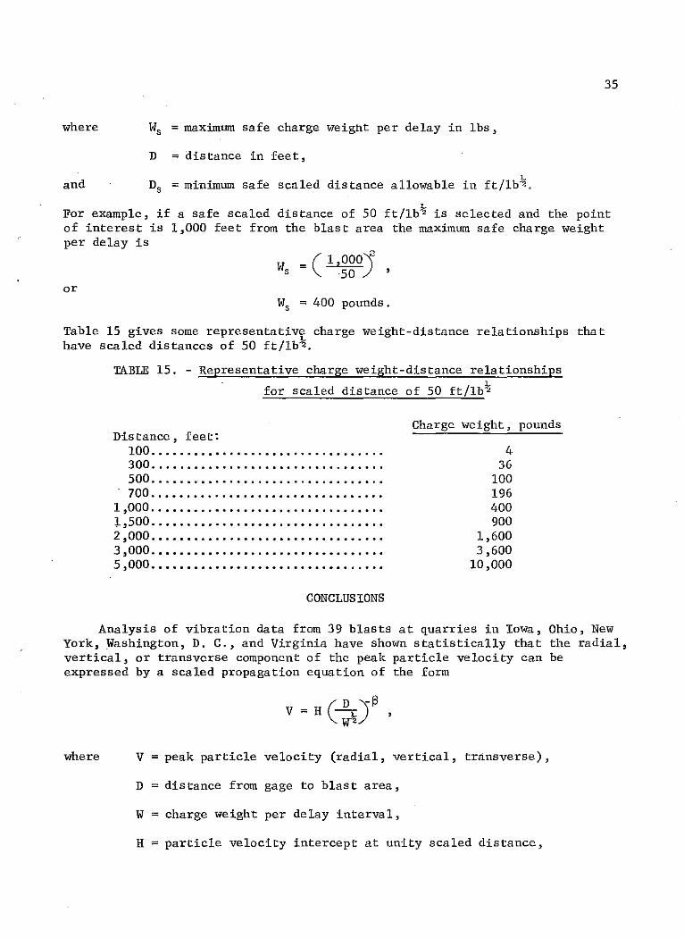
35

where W5 =maximum safe charge weight per delay in lbs,

D =distance in feet,

and D5 = minimum safe scaled distance allowable in ft/lb~.

For example, if a safe scaled distance of 50 ft/lb~ is selected and the point of interest is 1,000 feet from the blast area the maximum safe charge weight per delay is

= c 1 ,000)2

ws ·50 ' or

W5 = 400 pounds.

Table 15 gives some representative charge weight-distance relationships that ], have scaled distances of 50 ft/lb2,

TABLE 15. - Representative charge weight-distance relationships 1

for scaled distance of 50 ft/lb'>

Distance, feet: 100 0 0 0 0 0 0 0 0 0 0 • 0 0 0 0 0 0 0 0 0 0 0 0 0 • 0 0 0 0 ••••

300o 0. 0 .. 0 0 .... 0. 0. 0 0 ..... 0. 0 ... 0 0 ••

500. 0 0 0 • 0 • 0 0 • 0 • 0 0 •• 0 0 0 0 0 • 0 0 • 0 • 0 0 0 0 ••

700 0 0 0 0 0 • 0 0 0 0 • 0 0 • 0 0 • 0 0 0 0 0 0 0 0 • 0 • 0 • 0 • 0

1 ,ooo. 0 0 0 0 0 0 • 0 0 0 0 0 0 0 0 0 0 0 0 0 0 0 0 • 0 0 0 0 0 0 0 0

l ,500 0 0 0 0 0 0 0 0 0 0 0 0 0 0 0 0 0 0 • 0 0 0 0 0 • 0 0 0 0 0 0 • 0

2 , 000 0 0 0 0 0 0 0 • 0 0 • 0 0 0 0 0 0 0 0 0 0 0 0 0 0 0 0 0 0 0 0 0 0

3 '000 0 0 0 0 0 0 0 0 0 0 • 0 0 0 0 • 0 0 0 0 0 0 0 0 0 0 0 0 0 0 0 0 0

5 , 000 0 0 0 0 0 0 0 0 0 0 0 0 0 • 0 0 0 0 0 0 0 0 0 0 0 0 0 0 • 0 0 0 0

CONCLUSIONS

Charge weight, pounds

4 36

100 196 400 900

1,600 3,600

10,000

Analysis of vibration data from 39 blasts at quarries in Iowa, Ohio, New York, Washington, D. C., and Virginia have shown statistically that the radial, vertical, or transverse component of the peak particle velocity can be expressed by a scaled propagation equation of the form

(. D )~ v =H\.w~ ,

where V =peak particle velocity (radial, vertical, transverse),

D =distance from gage to blast area,

W =charge weight per delay interval,

H =particle velocity intercept at unity scaled distance,

36

and ~ = slope of particle velocity-scaled distance data on a log-log plot (~is constant for each component at a site, but may vary from site to site).

For a given distance, D, a scaled distance, D/W~, of 50 can be used to determine the maximum charge weight per delay without the use of seismic instrumentoat-ion. If lar,;er eha10ge weights per delay are needed, vibration measurements should be made to determine if the safe vibrations level will be exceeded.

REFERENCES

1. Duvall, Wilbur I., James F. Devine, Charles F. Johnson, and Alfred V. C. Meyer. Vibrations From Blasting at Iowa Limestone Quarries, BuMines Rept. of Inv. 6270, 1963, 28 pp.

2. Duvall, Wilbur I., Charles F. Johnson, Alfred V. C. Meyer, and James F. Devine. Vibrations From Instantaneous and Millisecond-Delayed Quarry Blasts. BuMines Rept. of Inv. 6151, 1963, 34 pp.

3. Duvall, Wilbur I., and David E. Fogelson. Review of Criteria for Esti­mating Damage to Residences From Blasting Vibrations. BuMines Rept. of Inv. 5968, 1962, 19 pp.

4. Johnson, Charles F. Coupling Small Gages to Soil. Earthquake Notes, Deptember 1962, pp. 40-47.

5. Ostle, B. Statistics in Research. Iowa State College Press, Ames, Iowa, 1956, pp. 133-137.

37

INT.~BU,OF MINES,PGH.,PA. 9477

-----------~---------~---- -------- ----------------------

•