Comput MechDOI 10.1007/s00466-012-0802-y

ORIGINAL PAPER

Effect of 3D grain structure representation in polycrystalsimulations

Devin M. Pyle · Jing Lu · David J. Littlewood ·Antoinette M. Maniatty

Received: 24 May 2011 / Accepted: 15 September 2012© Springer-Verlag Berlin Heidelberg 2012

Abstract Simulation results from finite element modelsusing two types of 3D polycrystal geometric representa-tions, one with a voxel representation and stair-stepped grainboundaries and the other with smooth grain boundaries, arecompared. Both models start with a periodic grain structurerepresentation, which is in the form of a regular, rectangular3D array of points, where each point is assigned an orien-tation. The voxel representation is obtained by simply sam-pling the array of grid points on a coarser regular grid witha prescribed resolution and forming a voxel centered at eachgrid point, which is assigned the grain orientation from thesampled grid point. The voxel representation may be mesheddirectly by decomposing each voxel into finite elements. Inthe second case, a method is presented that extracts geomet-ric topology information for a grain structure with smooth,flat grain boundaries from the discrete grain structure repre-sentation. From the geometric topology information, a finiteelement mesh is created. The two representations are then

D. M. Pyle · J. Lu · D. J. Littlewood · A. M. Maniatty (B)Department of Mechanical, Aerospace, and Nuclear Engineering,Rensselaer Polytechnic Institute, Troy, NY 12180-3590, USAe-mail: maniaa@rpi.edu

D. M. Pylee-mail: pyled@rpi.edu

J. Lue-mail: Jing.Lu@sbmoffshore.com

Present Address:J. LuSBM Atlantia, Houston, TX, USA

D. J. Littlewoode-mail: djlittl@sandia.gov

Present Address:D. J. LittlewoodSandia National Laboratories, Albuquerque, NM, USA

subjected to large strain deformations, and the simulationresults and efficiencies are compared. The macroscopicbehavior, overall texture evolution, and statistical distribu-tion of stress and slip are found to be nearly identical for bothmodels. However, noticeable differences are observed in themisorientation distribution within grains and the smoothnessof the stress field. The voxel representation is found to bemore efficient because of the uniform finite element mesh.

Keywords Crystal plasticity · Finite element method ·Polycrystal · Topology

1 Introduction

The macroscopic, mechanical behavior of polycrystallinemetals is dictated by underlying smaller scale phenomenaoccurring over a range of scales. One of the most informa-tive scales, in this multiscale perspective, is the grain scale.At the grain scale, important characteristics of the micro-structure, such as grain size, shape and orientation distribu-tion, are evident. These characteristics are strongly relatedto the macroscale behavior, both during processing of themetal and in-service. For example, the initial microstructure,before thermal-mechanical processing, has a strong impacton the final microstructure and also influences the deforma-tion behavior. In-service, the grain structure characteristicsaffect the anisotropy, strength, and ductility. It should also bementioned that the grain scale is not the only important scale,and that for a grain scale constitutive model to be accurate, itshould be based on smaller scale phenomena, in particular,dislocation phenomena.

Because of the importance of the grain scale in devel-oping predictive models of the behavior of metallic mate-rials, numerous researchers have developed approaches for

123

Comput Mech

modeling polycrystals. That work can be divided into twocategories: (a) models that assume a homogeneous deforma-tion and stress within each grain and take the macroscopicdeformation and stress to be the average over all the grains,which allow the grains to be modeled without an explicit rep-resentation, and (b) models that explicitly represent the grainstructure in order to capture the heterogeneous deformationand stress fields that occur within grains due to interac-tions with neighboring grains. Examples of the first categoryinclude: the Taylor model [1–3], where each grain is assumedto undergo the macroscopic deformation; the relaxed con-straint model for distorted, elongated grains [4,5], where themacroscopic deformation is prescribed along some direc-tions and the macroscopic stress is prescribed along otherdirections in the flat part of the grains; and self-consistentapproaches [6], where each grain is treated as embedded ina homogeneous equivalent medium. While these approachesprovide useful predictions regarding texture evolution andmacroscopic stress–strain response, they do not capture theintra-grain heterogeneities, which are important contribu-tors to certain physical processes and considered in the sec-ond category of polycrystal models. For example, grain sizeeffects are attributed to gradients in deformation fields thatarise in grains due to interactions with neighboring grains, seefor example Fleck and Hutchinson [7], Beaudoin et al. [8],and Janssen et al. [9]. The formation of nucleation sites forrecrystallization results from portions of a single grain rotat-ing into different orientations due to constraints imposed bysurrounding grains leading to low angle grain boundaries,see for example Beaudoin et al. [10] and Sarma et al. [11].Fatigue crack initiation may occur at grain boundaries or con-stituent particles and is related to the local grain orientations[12]. For a more comprehensive review of crystal plasticitymodeling, Roters et al. [13] provides an excellent overviewof constitutive models and multiscale methods for modelingcrystalline materials.

In order to capture the heterogeneous fields arising withinthe grains of a polycrystal, many researchers explicitly modelthe grain structure, most commonly using finite element dis-cretizations of polycrystals. Of the explicit polycrystal mod-els, a number of different geometric representations of thepolycrystals have been considered. The simplest approachuses uniform brick elements, where each brick may consti-tute a single grain [14,15], or where groups of brick ele-ments are defined as grains [11,16–18]. The former case isnot sufficiently refined to capture local variations that occurwithin grains. The latter case results in stair-stepped grainboundaries if irregular grain shapes are modeled. The natu-ral question that arises with regard to the latter approach iswhether such a topological representation, where the grainboundaries are stair-stepped, might lead to inaccurate results,especially near the grain boundaries, which may be a regionof key importance. A regular mesh may also be used to model

irregular grain structures, where the orientations are definedat the integration points instead of the grain boundaries,which eliminates the stair-stepped nature but does not createsmooth grain boundaries [19]. An alternate approach that al-lows for multiple finite elements within a grain to captureintragranular field variations without stair-stepped bound-aries is to model regular arrays of uniformly shaped grains.In Beaudoin et al. [8], groups of brick elements in a uni-form grid are distorted to form Wigner–Seitz cells. Ritz andDawson [20] compare the stress distributions resulting fromfour different regular grain representations, where groups oftetrahedral elements were used to form grains of cubic, rhom-bic, dodecahedral, and truncated octahedral shapes. In thatwork, similar trends were observed in the stress distributionsacross the geometric representations, but with differences inthe level of intra- and inter-granular variability because ofdifferences in levels of geometric constraint. These meth-ods provide a smooth, more accurate representation, but thegrains are still uniform and regular, and thus, the naturalvariability of the grain structure is not captured. In recentyears, researchers have used Voronoi tesselations to definethe grain structure and then meshed with tetrahedral elements[21–24]. However, the grain representations produced bystraight Voronoi tesselations are not as accurate as thosedefined using methods described in the next paragraph, whichgenerate typically a regular, rectangular grid of points, whereeach point is assigned an orientation.

There are many methods to generate grain structuresbased on the approach of simulating the phenomenon ofgrain growth. The popular ones are the Monte Carlo (Potts)[25,26], phase field [27], and cellular automaton [28] meth-ods. Each of these methods treat microstructures as thermo-dynamically unstable, and evolve the microstructure with thegoal of minimizing total free energy. The microstructure rep-resentations that result from these models are typically a reg-ular grid of points in 3D space, with each point assigned anorientation, and where groups of neighboring points with thesame orientation constitute a grain. An alternative approachto these methods, which is not based on grain growth, butrather seeks to directly represent the grain structure, also as aregular grid of points in 3D space, with a statistically similarrepresentation is described by Saylor et al. [29]. A similarapproach is used in St-Pierre et al. [30], where the represen-tative volume is filled with non-overlapping ellipsoids withthe size and aspect ratio distributions found from experimen-tal observations, and then the space is filled by grid points,where each grid point is assigned to a grain based on whatellipsoid it lies in or is closest to. Finally, it should also bementioned that 3D grain structure representations of actualgrain structures may be obtained experimentally using elec-tron backscatter diffraction (EBSD) to image a series of 2Dslices, where a focused ion beam (FIB) is used to removematerial between successive 2D slices [23,24,31] or through

123

Comput Mech

3D X-Ray diffraction [32]. This also typically generates a3D regular grid representation of the grain structure.

The present work compares the results of explicit poly-crystal simulations for two different topological represen-tations, one with a voxel representation with stair-steppedgrain boundaries, which we will refer to as voxel topology(VT) and one where the polycrystals have smooth, flat grainboundaries, which we will refer to as smooth topology (ST).A similar comparison was presented in Kanit et al. [21] fora two-phase, linear, elastic material, where each phase wasisotropic, and they found that in small models the averageresults for stress and strain matched, and field fluctuationsdiffered slightly. In this work, we consider large strains inanisotropic, elasto-viscoplastic polycrystals. We also pres-ent a procedure for creating the smooth grain boundary rep-resentation from the regular grid data that allows for finiteelement meshing. For both implementations, we start with amodified Monte Carlo (Potts) model, based on that presentedin Radhakrishnan and Zacharia [26], for generating the sim-ulated grain structure represented by a regular array of gridpoints, where each point is assigned an orientation. Here, themodel is modified to generate a periodic microstructure. Cur-rently, this work is limited to relatively equi-axed grains of asingle phase material, which this procedure generates. Next,we apply a procedure for removing small features based onprescribed criteria. The VT model can be created directly bysampling the grid points on a grid of the same or coarser res-olution, creating a voxel centered at each sampled grid point,and sub-dividing each voxel into finite elements. Afterthis, we present an approach for extracting topology informa-tion, specifically vertices, edges, patches, and regions, whichis used to define the ST geometric model of the grain struc-ture. A standard 3D finite element mesher can be used giventhe topology information. The VT and ST models are gen-erated so that the number of elements in the resulting finiteelement meshes for each topological representation are com-parable allowing for direct local comparisons to be made.Both models are then deformed to a large strain (20 % planestrain compression), and the resulting orientation, misorien-tation, stress, and slip fields are compared between the mod-els, and conclusions are drawn. The relative computationalefficiency of each model is also compared.

2 Generating polycrystal models

In order to compare the results of simulations with voxel andsmooth topologies, it is first necessary to define compara-ble models. A data set of orientations assigned to a regulararray of grid points representing a polycrystal is required first.Here, a modified Monte Carlo approach, described next, isused to define the initial data set defining the model poly-crystal, however, any approach that creates a regular grid

array polycrystal representation may be used as a startingpoint. After that, the VT and ST representations and asso-ciated finite element meshes are created. The approach foreach is described below.

2.1 Modified Monte Carlo simulation

The first step in generating the polycrystal representationsinvolves creating a 3D polycrystal unit cell using a modifiedMonte Carlo grain growth algorithm based on that presentedin Radhakrishnan and Zacharia [26], which is summarizedhere. First, a 3D structured grid point domain of N × N × Nis chosen, with each grid point in the domain given a uniqueorientation number. Then, in each step of the simulation, onegrid point is chosen randomly, and its orientation switchedto that of a nearest neighbor randomly selected. The energychange of the local cluster associated with this switchingis then calculated. If the local cluster energy is lowered, thenew orientation is kept; otherwise, the orientation is switchedback to its previous value. The local cluster energy is calcu-lated using

E = −J

⎡⎣

n∑j=1

δs0s j

⎤⎦ (1)

where J is a constant being proportional to the grain bound-ary energy, δi j is the Kronecker δ function, S0 is the orien-tation number of the grid point whose orientation change isbeing attempted, S j is the orientation number of a nearestneighbor, and n is the number of nearest neighbors, 26 in ourcase. The goal of the microstructure evolution is to reducegrain boundary energy. Intuitively, we can imagine that thegenerated grain structures will be of convex shape with flatfacets and straight edges since that is the most efficient way ofconstructing grains. Furthermore, since this energy functionis isotropic, the grains will be on average equi-axed.

The evolution is counted by the Monte Carlo Steps (MCS),where each Monte Carlo Step is N × N × N orientationswitching attempts. The grain growth continues until thenumber of remaining grains reaches a specific value. In orderto link to the macro-scale, these polycrystals are designed tohave periodic boundaries by assuming opposite faces of thepolycrystal are linked and neighboring each other. In thiswork, a generated microstructure with 107 grains and 180regions, comprised of 200×200×200 grid points is created.There are more geometric regions than grains due to period-icity, i.e., the grains wrap around to the opposite side of thegeometric model splitting the grain into multiple regions.

2.2 Small feature elimination

Before extracting the two topological representations con-sidered here, for simulation efficiency, small features in the

123

Comput Mech

Small volume

Fig. 1 2D sketch showing three types of small features

model should be eliminated or reduced as much as possible.The small features may include small grains generated by theMonte Carlo grain growth simulation (if the modeler decidesthese are not important), and small volume and high aspectratio portions generated by periodic unit cell boundaries cut-ting through grains on the boundary (Fig. 1). The positionsof the periodic unit cell boundaries are adjusted so that theleast number of small features are created. Since the poly-crystal example described here is made up of 200×200×200grid points, there are 200 possible locations for the periodicboundaries in each of the three dimensions. All 200 possi-ble positions are tested in each dimension and the optimalpositions chosen.

2.3 Geometric model representations

Two different geometric representations of the polycrystalmodel are considered and meshed for finite element simula-tion. The VT and ST models are meshed with similar numbersof quadratic, tetrahedral elements for comparison, and threemeshes are created for each model in order to test for meshconvergence as well as to investigate simulation efficiency.The meshes are designed to have roughly 1,000; 1,300 and1,800 elements per grain. First, the simpler voxel topologymodel is described briefly, and then a method is presented togenerate the smooth topology model.

2.3.1 Voxel topology model

The voxel topology (VT) model is relatively straightforwardto create and mesh once the discrete model is generated. Inthis work, in order to create finite element models with acomparable number of elements to compare to the smoothmodels, we sample the grid points generated from the MonteCarlo procedure, with 200 grid points along each direction,onto coarser grids to define the VT model. In order to ob-tain the desired number of elements per grain, as mentionedabove, we choose three grid sizes, with 26, 29, and 32 gridpoints along each direction. The center of each sampled gridpoint is taken as a voxel center, and the voxel boundariesare centered between sampled grid points. Each voxel is as-signed the grain orientation identity of the grid point at itscenter. Meshing this topology involves simply meshing each

voxel. Here, each voxel is divided into 6 congruent, qua-dratic, tetrahedral finite elements, resulting in meshes with105,456 elements, 146,334 elements, and 196,608 elements.This method also naturally aligns the nodal points on oppos-ing faces allowing for these nodes to be constrained if peri-odic boundary conditions are used. The three VT modelscreated are shown in Fig. 2.

2.3.2 Smooth topology model

A procedure for extracting a smooth topological represen-tation from the discrete 3D regular, rectangular grid repre-sentation was developed and used in this work. The approachtaken here is based on the well-known Marching Cubes algo-rithm [33] used widely in the field of visualization. Construct-ing geometric topology from 3D scalar fields is sometimesreferred to as “3D surface reconstruction” or “polygoniz-ing 3D scalar fields” [34]. In visualization applications, itis not critical to avoid overlap or penetration, which mayoccur with the Marching Cubes algorithm, but overlap orpenetration is a problem for constructing a finite elementmodel. Numerous methods have been developed to overcomethis problem, including the modified Marching Cubes [35],Marching Tetra-cubes [36] and Marching Intersections [37]methods. In Wiederkehr et al. [38], the modified MarchingCubes method is used, following the procedure developedin [35,39] to generate a consistent topology of a microstruc-tural representation, which is subsequently meshed for finiteelement analysis. Here, a fairly simple approach is devisedthat focuses on the voxels lying at the grain boundaries. Thefirst step is to sift out the boundary cubes, where each cubeis defined by eight grid points that make up the corners ofthe cube, each with an assigned orientation from the MonteCarlo procedure. Boundary cubes are the cubes that lie on theboundary between grains, having grid points of different ori-entation values. It is these boundary cubes that collectivelyrepresent the interfaces between different grains, and pro-vide the basis for geometric model construction. There aretwo important properties associated to each boundary cube:the x, y, and z coordinates of the weighted center of the eightgrid points of this cube (that will be used as the location of thegeometric entity), and the orientations of the grid points atthe corners of the cube (which provides connections betweenboundary cubes). The weighted center of a boundary cube isfound by partitioning the eight grid points of the cube by theirorientations, finding the center of each group with a commonorientation, defining the weight for each group as the fractionof the eight grid points that has that common orientation, andthen adding the center of each group multiplied by its weight.

The boundary cubes are organized into geometric entities(vertices, edges, patches, regions) by considering the numberof different orientations associated with the grid points defin-ing each boundary cube. Interfaces (grain boundaries) are

123

Comput Mech

(a) (b) (c)

Fig. 2 Three VT model representations with a 26 voxels, b 29 voxels, and c 32 voxels, along each edge

at locations where two regions (i.e., two grain orientations)meet, edges at locations where three regions meet, and verti-ces at locations where four or more regions meet. Since thepolycrystal models are generated with the goal of reducinginterfacial regions, the above simple rules are well followed.Technically, it is possible to have an edge where four regionsmeet, but those cases are energetically unfavorable (in thesense of creating unnecessary grain boundary regions), andrarely occur. In fact, such a case has not been observed in ourmodels and is typically not seen in real microstructures ofsingle phase materials, where grains are normally observedto meet at triple points in 2D sections (which corresponds tothree grains meeting to form an edge) and not at quadruplepoints (which would correspond to four grains meeting at anedge), see, for example, Cahn [40].

First, the vertices are identified followed by the edgesthat connect them. The weighted center point of these vertexcubes is regarded as the vertex location. Edge cubes con-taining the same three orientations are on the edge wheregrains with those three orientations meet. Since these threeorientations are also associated with the vertices on the twoends of the edge, the two end vertices can be found and anedge is created by connecting these two vertices (Fig. 3). Totest the accuracy of using this straight line to represent thereal edge made up of edge cubes, the distance from each ofthe edge cubes associated with this edge to the created edgeis calculated and the maximum distance is defined as the“error” of this edge (Fig. 4). Here, we choose 1.0 (the dis-tance between neighboring grid points) as the critical “error”value, where a typical edge is made up of more than ten edgecubes. If the error of an edge is smaller than 1.0, we regard itas straight and keep the edge created by connecting the twovertices, otherwise, we split the edge into two straight edgesby inserting a new vertex at the location of the edge cubehaving the maximum error. Typically, only about 10 % of theedges created have an “error” larger than 1.0, meaning thatmost of the edges are straight, and that the previous assump-tion (that all interfaces are of 3D polygon shape) is valid. The

Fig. 3 2D sketch showing edge creation based on corresponding edgecubes and vertex cubes. Shaded cubes are vertex cubes, others are edgecubes

Fig. 4 2D sketch showing edge-split operation used to increase theaccuracy of the constructed edge. Shaded cubes are vertex cubes, othercubes are edge cubes

splitting procedure was only applied once to avoid creatingshort edges.

Similarly, interface cubes with the same two orientationvalues collectively form an interface, and the two orienta-tion values are also associated with the edges enclosing theinterface. Edges associated with this interface are found inorder to form an edge loop. If all the edges are lying on thesame plane, this interface is a patch; otherwise this inter-face is triangulated by either introducing a vertex aroundthe center of the interface, or just connecting the existingvertices (Fig. 5). All possible splitting choices are tested,and the one which maximizes the minimum angle of allthe angles of the triangulation is used. It should be notedthat this procedure assumes flat interfaces, taking advan-tage of the fact that flat interfaces are energetically favor-able. If the interfaces between the grains are not flat, error isintroduced.

123

Comput Mech

Fig. 5 Two ways of triangulation: a by introducing a new vertex; b byconnecting existing vertices

After all patches are constructed, the region-patch connec-tion is established by tracing the common orientation valuesbetween regions and patches. The complete geometric struc-ture is constructed and no further polishing is needed.

A 3D mesh is then generated using Abaqus FEA software[41]. Because of the periodicity of the grain structure, whilethere are twelve edges on the polycrystal model, there areonly three unique edge discretizations. For example, all ofthe edges parallel to the x axis cut through the same grainsand have the same discretization. Thus, each of the threeindependent edges is meshed first with 1D meshes that arethen copied to remaining edges. Next, three sides sharing onecorner of the unit cell are each given a surface mesh, wherethe mesh is seeded by the discretization already done on theedges. The surface mesh is then copied to the three remainingopposite sides so that periodic boundary conditions may beeasily applied by constraining matching nodes on oppositefaces. Finally the interior volume is fully meshed, insuringperiodicity. Three meshes were created with varying levelsof refinement: 104,165; 146,918; and 194,297 elements. Fig-ure 6 shows the resulting meshed grain structure, comparingthe meshed VT model described in the preceding Sect. (2.3.1)and the ST model described here with the finest meshes usedin this work, that is with 196,608 and 194,297 elements,respectively.

3 Material model

The grain-scale constitutive model used in the finite elementimplementation is presented in this section. In this work, alu-minum alloy 7075-T651 is modeled, which is a face-centeredcubic (fcc) metal with twelve primary {111}〈110〉 slip sys-tems. The derivation of the constitutive model along withthe calibration of material parameters is given in [42], and asummary is presented here. The tensor notation used hereinfollows that in Gurtin [43]. First, a multiplicative decompo-sition of the deformation gradient into its elastic and plasticparts [44] is assumed

F = F eF p (2)

where F p is the plastic deformation gradient and F e is theelastic deformation gradient. The Green-Lagrange elasticstrain tensor is then E

e = 12 (F eT F e − I ).

A hyperelastic potential is used for the elastic response.Specifically, the following simple quadratic form is used

W (Ee) = 1

2E

e · L[Ee] (3)

where L is the fourth order elasticity tensor, which is definedin terms of the three independent elasticity parameters forcrystals with cubic symmetry, C11, C12, and C44, and theˆ indicates the relaxed, elastically unloaded configuration.The second Piola-Kirchoff stress, S is then

S = ∂W

∂Ee = L[Ee] (4)

and the Cauchy stress, σ , on the deformed configuration is

σ = 1

det (F e)F eSF eT . (5)

For the viscoplastic response, the rate of shearing, γ α , istaken to be related to the resolved shear stress, τα , on the α

slip system through a power law

γ α = γ0τα

gα

∣∣∣∣τα

gα

∣∣∣∣1/m−1

(6)

where γ0 is the reference shearing rate, m is the strain ratesensitivity, and gα is the slip resistance. The resolved shearstress on a slip system is related to the second Piola-Kirchhoffstress through

τα =(F eT F eS

)· P

α, P

α = (sα ⊗ m

α)

(7)

where Pα

is the Schmid tensor defined in terms of the slipdirection and slip plane normal, s

α and mα , respectively, for

slip system α. The relationship between the plastic defor-mation gradient and the rate of shearing on the slip systemsis

Lp = F

p(F p)−1 =

Ns∑α=1

γ αPα

(8)

where Lp

is the plastic velocity gradient. The resistanceto plastic slip, gα , which describes the hardening behavior,evolves according to

gα = G0

(gs − gα

gs − go

) Ns∑β=1

Hαβ |γ β | (9)

where g0 is the initial slip resistance on all the slip systems,G0 is the hardening rate coefficient, gs is the saturation hard-ness, and Hαβ is the slip interaction matrix which describesthe relative strength of latent and self hardening on the slip

123

Comput Mech

(a) (b)

Fig. 6 Meshed 107 grain structure: a voxel topology and b smooth topology

systems. In this work, we model aluminum alloy 7075-T651,which is a dispersion strengthened alloy, where hardening isassociated with dislocations bowing out and forming loopsaround precipitates. Hardening is caused by incompatibili-ties between the plastic strain field due to slip and the elasticprecipitates. The resulting form of the hardening matrix is

Hαβ =∣∣∣Mα · L

[(Y − I

)[Mβ ]

]∣∣∣ (10)

where Mα

is the symmetric part of the Schmid tensor, P α, Yis the average Eshelby tensor associated with the precipitates(approximated as elliptical), and I is the fourth order identitytensor. For details of the model derivation and calibration ofmaterial parameters, see Bozek et al. [42]. The model param-eters for AA7075-T651 are given here in Tables 1 and 2 forcompleteness.

4 Finite element implementation

The model is implemented in parallel into a 3D finite ele-ment framework using an integration algorithm describedin [45] and a finite element formulation with a consis-tent tangent similar to that described in [46]. A mixeddisplacement/pressure finite element formulation is usedwith P2/P1 tetrahedral elements, specifically quadratic dis-placement interpolation and linear, discontinuous pressureinterpolation. The pressure is eliminated at the elementlevel so that the nonlinear finite element procedure onlysolves for the displacement degrees of freedom. Periodicboundary conditions are implemented where the formu-lation is defined in terms of the displacement fluctuationfield with the fluctuations constrained to match on opposite

faces [47], effectively treating the modeled unit cell as rep-licated on each side. For information regarding specificdetails of the integration algorithm, finite element imple-mentation, or derivation of the consistant tangent, see [48].The open source software toolkit PETSc is used for par-allel solution of the resulting equations using the conju-gate gradient method with a block Jacobi pre-conditioner[49].

5 Simulation results

In order to compare the VT and ST representations, we modelplane strain compression to a 20 % reduction over 20 secondsin the 107 grain structure. The deformation is defined suchthat the material is compressed along ND, lengthened alongRD, and TD is the zero strain direction, as typical for rolling.The grain structure was assigned a set of random orienta-tions. The VT and ST models are shown in Fig. 7 withoutmeshes, where the colors indicate the grain orientations usingthe inverse pole figure color map shown.

5.1 Mesh convergence and efficiency

As mentioned before, the VT and ST models were meshedwith similar numbers of quadratic, tetrahedral elements forcomparison, and three meshes were created for each modelin order to test mesh convergence as well as to investigatesimulation efficiency. Table 3 lists the number of elementsand degrees of freedom for each model.

For checking mesh convergence, we only look at the dif-ference in results between the different meshes for each

123

Comput Mech

Table 1 Material parametersfor AA7075-T651 m γ0 (s−1) g0 (MPa) G0 (MPa) gs (MPa) C11 (GPa) C12 (GPa) C44 (GPa)

0.005 1.0 220 120 250 107.3 60.9 28.3

Table 2 Hardening interactionmatrix (Hαβ ) and slip systemnumbering

Slip System ID 1 2 3 4 5 6 7 8 9 10 11 12

(111) [110] 1 1.0 0.50 0.50 0.50 0.59 0.088 0.088 0.50 0.59 0.18 0.088 0.088

(111) [101] 2 0.50 1.0 0.50 0.59 0.50 0.088 0.18 0.088 0.088 0.088 0.59 0.50

(111) [011] 3 0.50 0.50 1.0 0.088 0.088 0.18 0.088 0.59 0.50 0.088 0.50 0.59

(111) [101] 4 0.50 0.59 0.088 1.0 0.50 0.50 0.59 0.50 0.088 0.088 0.18 0.088

(111) [110] 5 0.59 0.50 0.088 0.50 1.0 0.50 0.088 0.088 0.18 0.59 0.088 0.50

(111) [011] 6 0.088 0.088 0.18 0.50 0.50 1.0 0.50 0.59 0.088 0.50 0.088 0.59

(111) [101] 7 0.088 0.18 0.088 0.59 0.088 0.50 1.0 0.50 0.50 0.50 0.59 0.088

(111) [011] 8 0.50 0.088 0.59 0.50 0.088 0.59 0.50 1.0 0.50 0.088 0.088 0.18

(111) [110] 9 0.59 0.088 0.50 0.088 0.18 0.088 0.50 0.50 1.0 0.59 0.50 0.088

(111) [110] 10 0.18 0.088 0.088 0.088 0.59 0.50 0.50 0.088 0.59 1.0 0.50 0.50

(111) [101] 11 0.088 0.59 0.50 0.18 0.088 0.088 0.59 0.088 0.50 0.50 1.0 0.50

(111) [011] 12 0.088 0.50 0.59 0.088 0.50 0.59 0.088 0.18 0.088 0.50 0.50 1.0

(a) (b)

111

101001

(c)

Fig. 7 107 grain models used in the simulations for comparison where the grain orientations are depicted with an inverse pole figure color mapwith respect to the ND sample direction: a VT model, b ST model, and c inverse pole figure color map legend

model representation type (VT and ST), and in the nextsection we will compare the VT and ST results with eachother in more detail. First, we consider the difference in thegrain sizes between the different representations. The STmodels all have exactly the same grain sizes because theyare based on the same geometric model. The differences ingrain sizes between the VT and ST models relative to theaverage grain size are 1.58, 1.34, and 0.97 % on average, forthe coarsest to finest VT models, with maximum differencesof 6.89, 6.24, and 4.30 %.

The variability in the stress is an important quantity thatwe study here, and so we will first look at the average andstandard deviation in the stress for the different meshes. Theresulting volume average and standard deviation in the von

Mises effective stress for each mesh is given in Table 3 at 15and 20 % compression. The von Mises effective stress is firstcomputed in each element and then the volume average andstandard deviation in the von Mises stress are evaluated forthe polycrystal. The results for individual stress componentsare similar, with the difference in average and standard devia-tion in the stress between the finest and the intermediate meshless than 1.5 and 2.2 MPa, respectively, and between the fin-est and coarsest mesh less than 2.5 and 3 MPa, respectively,for any stress component. It should be noted that no valuesare given in Table 3 for 20 % compression for the coarsestST mesh because the simulation failed at 18 % compressiondue to element distortion, which is explained in more detailbelow.

123

Comput Mech

Table 3 Mesh convergence study data at 15 and 20 % compression(dof number of degrees of freedom)

No. elements dof 15 % 20 %

σ (MPa) σ (MPa) σ (MPa) σ (MPa)

Voxel

105,456 446,631 670.5 101.2 683.4 103.1

146,334 616,137 669.3 100.7 682.7 102.3

196,608 823,875 668.3 100.5 681.5 102.4

Smooth

104,165 434,274 666.3 99.0

146,918 605,187 665.0 98.7 677.3 100.6

194,297 794,664 664.4 98.3 677.0 100.2

Comparison of average (σ ) and standard deviation (σ ) in the vonMises effective stress

The total slip on the slip systems is also an interesting localmetric, which will be high in regions of localized deforma-tion. The total slip γ T is computed locally as

γ T =Ns∑

α=1

t f∫

0

∣∣γ α∣∣ dt (11)

where t f is the time at the end of the simulation. First, welook at the distribution of slip over the polycrystal at the endof the deformation (20 % compression), where the total slipin each element is weighted by the element volume. Figure 8compares the distributions for the middle and finest meshesfor the (a) VT models and the (b) ST models. We see thatthe distributions are not significantly different between thetwo meshes. In fact, the mean and standard deviations forthe middle and fine meshes are identical in each case, andthe peak values are also close, changing by less than 5 %between the meshes. We also look locally at the total slipγ T on a 2D slice cut on an ND-RD plane near the center ofthe grain structure, where the total slip is interpolated ontoa regular 2D grid with 106 points along RD and 68 pointsalong ND, considering only interior points. Results for themiddle and finest meshes considered are shown in Fig. 9. Thegeneral pattern of the total slip is very similar between themiddle and fine meshes (Fig. 9a, b for the VT model, Fig. 9c,d for the ST model), and the difference in the slip betweenthe meshes is fairly small except near some grain boundaries(Fig. 9e, f). The median difference between meshes in totalslip is 9.3 % for the VT model and 4.5 % for the ST modelrelative to the average slip. This indicates that a finer mesh isneeded for the VT model to achieve the same level of accu-racy as the ST model, which is not surprising. Some of theerror between meshes is due to the interpolation onto a reg-ular grid, especially near grain boundaries where the error ishighest because the regular grid point may fall in differentgrains in the different meshes.

In addition to considering the difference in simulationresults between the two model representations, it is alsoimportant to consider simulation costs. Because the VT mod-els have initially uniform meshes and the element shapes areguaranteed to be optimal, the simulations with the VT modelare easier to set-up, run more efficiently, and are more robustthan ST models. The graph in Fig. 10 compares the efficiencybetween the two representations using the set of meshesdescribed above. The simulations were run on an IBM BlueGene L using 512 processors. From the graph, we see that theVT model is significantly more efficient for a similar numberof degrees of freedom. The slow down in the simulations asthe deformation progresses is due to the element distortion.Quadratic tetrahedral elements are used here for interpolat-ing the displacement field, which, due to the mid-side nodeson the element edges, can exhibit substantial local volumechange at large strains when the elements have a high aspectratio, even though the overall volume of the elements doesnot change substantially. It should be noted that elastic com-pressibility only is allowed, while the plastic deformation,which is the majority of the deformation, is assumed incom-pressible. When a relatively large volume change occurs atan integration point, the integration algorithm may not con-verge because it is designed for large, nearly incompressibledeformations, causing the step size to be cut leading to theslow down in the simulations as the deformation progresses.Ultimately, if the step size becomes too small, the simulationis ended, which is the case for the coarsest ST model thatfailed at about 18 % compression. Periodic remeshing mayimprove performance, but may also introduce error due tovariable remapping and the re-equilibration process. Lowerorder, e.g. linear elements in displacement and constant pres-sure, would be more robust, but would require greater meshrefinement for accuracy. A low-order stabilized method maybe a better approach, where robust and accurate P1/P1 (lineardisplacement and pressure) elements are used [50].

5.2 Voxel and smooth model result comparison

A number of different metrics are used to compare the re-sults for the two geometric representations of the same grainstructure. Here, we only compare the results between the VTand ST models obtained with the finest meshes considered(196,608 elements for the VT model and 194,297 elementsfor the ST model).

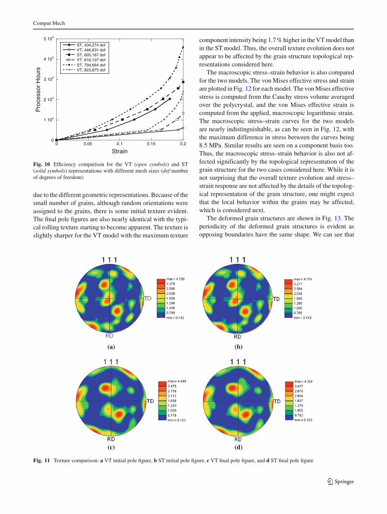
First, we compare the overall texture evolution in eachcase. The initial and final 〈111〉 equal-area pole figures areshown in Fig. 11. The pole figures are generated by weight-ing the orientation in each finite element by the size of theelement and computing the orientation intensities in each 5◦bin used to generate the pole figures. Not surprisingly, the ini-tial pole figures are nearly identical, with small differencesdue to the slight difference in volumes of the initial grains

123

Comput Mech

00 0.5 1 1.5 2 0 0.5 1 1.5 2

0.05

0.1

0.15

0.2

0.25Middle MeshFine Mesh

volu

me

frac

tion

slip range

(a)

0

0.05

0.1

0.15

0.2

0.25

volu

me

frac

tion

slip range

(b)Middle MeshFine Mesh

Fig. 8 Histograms showing distribution of total slip over entire polycrystal: a comparing the results for the VT models with 146,334 (middle mesh)and 196,608 (fine mesh) elements, and b comparing the results for the ST models with 146,918 (middle mesh) and 194,297 (fine mesh) elements

(a) (b)

(c) (d)

(e) (f)

1.5

1.0

0.5

0

1.5

1.0

0.5

0

0.5

0.45

0.4 0.35

0.3

0.25

0.2

0.150.1

0.05

0

Fig. 9 Total accumulated slip interpolated onto a regular grid on a 2Dslice, horizontal is RD, vertical is ND for different meshes and the dif-ference between meshes: a VT model, 146,334 elements, b VT model,

196,608 elements, c ST model, 146,918 elements, d ST model, 194,297,e difference between results shown in (a) and (b) for VT models,f difference between results shown in (c) and (d) for ST models

123

Comput Mech

0

1 104

2 104

3 104

4 104

5 104

0 0.05 0.1 0.15 0.2

ST, 434,274 dofVT, 446,631 dofST, 605,187 dofVT, 616,137 dofST, 794,664 dofVT, 823,875 dof

Pro

cess

or H

ours

Strain

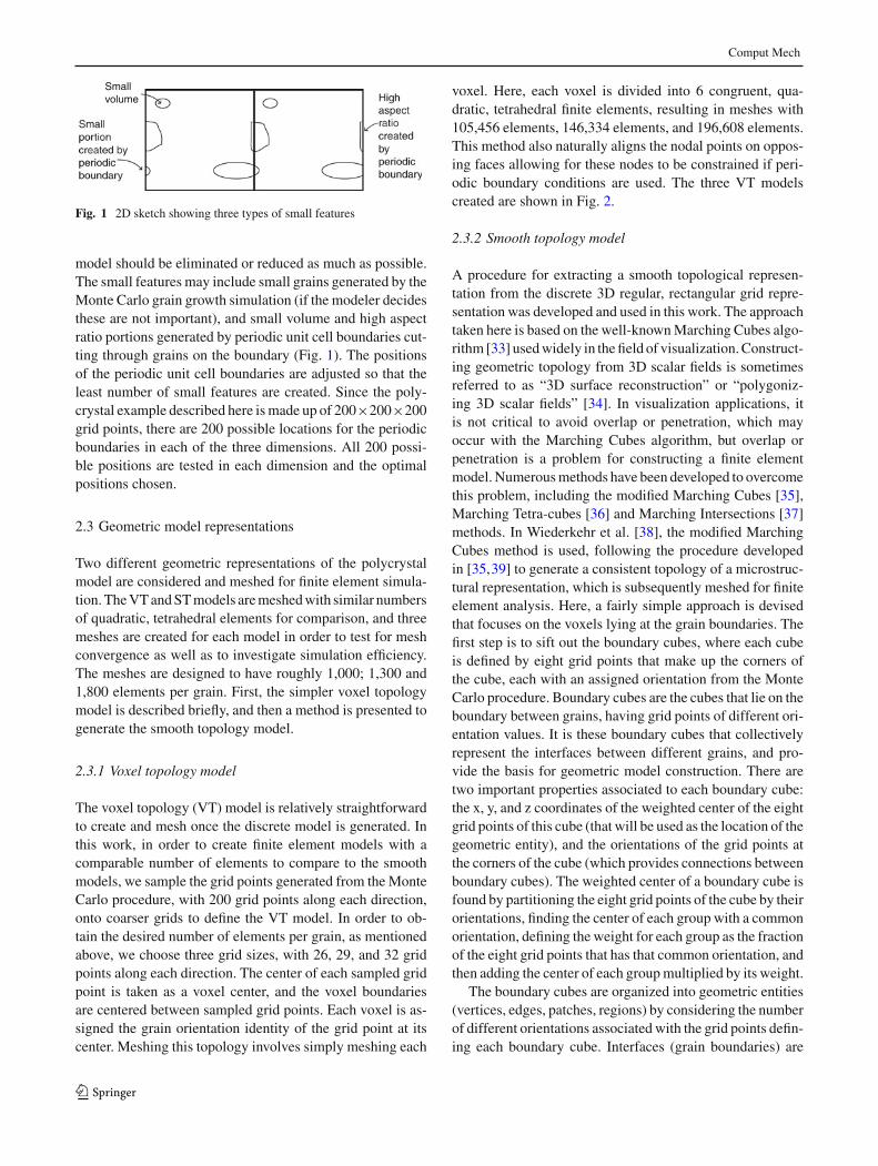
Fig. 10 Efficiency comparison for the VT (open symbols) and ST(solid symbols) representations with different mesh sizes (dof numberof degrees of freedom)

due to the different geometric representations. Because of thesmall number of grains, although random orientations wereassigned to the grains, there is some initial texture evident.The final pole figures are also nearly identical with the typi-cal rolling texture starting to become apparent. The texture isslightly sharper for the VT model with the maximum texture

component intensity being 1.7 % higher in the VT model thanin the ST model. Thus, the overall texture evolution does notappear to be affected by the grain structure topological rep-resentations considered here.

The macroscopic stress–strain behavior is also comparedfor the two models. The von Mises effective stress and strainare plotted in Fig. 12 for each model. The von Mises effectivestress is computed from the Cauchy stress volume averagedover the polycrystal, and the von Mises effective strain iscomputed from the applied, macroscopic logarithmic strain.The macroscopic stress–strain curves for the two modelsare nearly indistinguishable, as can be seen in Fig. 12, withthe maximum difference in stress between the curves being8.5 MPa. Similar results are seen on a component basis too.Thus, the macroscopic stress–strain behavior is also not af-fected significantly by the topological representation of thegrain structure for the two cases considered here. While it isnot surprising that the overall texture evolution and stress–strain response are not affected by the details of the topolog-ical representation of the grain structure, one might expectthat the local behavior within the grains may be affected,which is considered next.

The deformed grain structures are shown in Fig. 13. Theperiodicity of the deformed grain structures is evident asopposing boundaries have the same shape. We can see that

(a) (b)

(c) (d)

Fig. 11 Texture comparison: a VT initial pole figure, b ST initial pole figure, c VT final pole figure, and d ST final pole figure

123

Comput Mech

0

100

200

300

400

500

600

700

800

0 0.05 0.1 0.15 0.2 0.25

voxelsmooth

stre

ss (

MP

a)

strain

Fig. 12 The von Mises effective stress vs. strain for the two modelrepresentations

some of the grains are starting to break up with multipleorientations within the grains, shown by the color varia-tions in the figure. The figures look quite similar as far asthe overall shape of the deformed structure and the colorvariations appearing within the grains. The primary visi-ble difference is the “stair-steps” on the grain boundariesin the VT model. Qualitatively, the color variations in theST model appear to change more smoothly than in the VTmodel.

The primary purpose of modeling discretized grainstructures is in order to capture the local fluctuation in thedeformation from that of a uniform deformation. One wayto quantify the non-uniformity of the deformation is to com-pute the average fluctuation in the displacement field fromthat of a uniform deformation. The average fluctuation in thedisplacement field between the two models is found to differ

by less than 1 % here indicating that that average level oflocal fluctuations in both models is not substantially differ-ent.

To examine the spatial difference in the predictions ofhow the grains break up in each of the models more quan-titatively, we look at the intragranular misorientations thatdevelop within the grains. First, we look at the misorienta-tions on a 2D slice cut on an ND-RD plane, similar to theslice considered in Sect. 5.1 but at a slightly different loca-tion in the TD direction and zoomed in more to the interiorof the polycrystal. The orientations are interpolated onto aregular grid on the 2D slice. The kernel average misorienta-tion is then computed for each grid point using OIM AnalysisSoftware [51], where the kernel average misorientation is theaverage misorientation between that grid point and its neigh-bors excluding points with misorientations greater than 10◦so as not to include grain boundaries. It should be noted thatwe chose 10◦ instead of 15◦ here in order to better visualizethe misorientations in the central parts of grains. The mis-orientation is strongly dependent on the grid spacing. Here,the second nearest neighbor was used in computing the mis-orientations in order to avoid using grid points that may liewithin a single finite element.

The results are shown in Fig. 14 where the same colorscale is used. Some differences in the grain structures are adirect result of the differences between the VT and ST repre-sentations. Additional differences, however, result from theinfluence of the stair-stepped grain boundaries on texture evo-lution. Note, the small stair-steps appearing in the image forthe ST model result from the regular grid used by the OIMsoftware and do not represent the actual finite element meshused. For the ST model, the maximum misorientations appearat grain boundaries, which is not surprising as the grainsmay need to rotate differently near the grain boundaries fromthe interior in order to satisfy compatibility and equilibrium

(a) (b)

Fig. 13 Deformed 107 grain models used in the simulations for comparison where the grain orientations are depicted with the same ND inversepole figure color map as in Fig. 7: a VT model and b ST model

123

Comput Mech

A

B

(a)

B

A

(b)

Fig. 14 Misorientation distribution on a 2D slice: a VT model andb ST model. Horizontal is along RD and vertical is along ND. Smallstair-steps appearing in the ST model result from the regular grid used inthe OIM imaging software and do not represent the actual finite elementmodel used

across the grain boundary. However, in the VT model, thehighest misorientations do not seem to be as concentratednear grain boundaries. This may be due to the stair-steps at

the boundary locking the boundaries resulting in strongerkinematic constraints on the grain rotations than might natu-rally occur. The average and maximum misorientations on theplane for the VT model are 1.11◦ and 6.43◦, respectively, andfor the ST model, they are 1.19◦ and 7.68◦. Thus, the averageand maximum misorientations predicted on the plane for theST model are 7 and 19 % higher, respectively, than for the VTmodel. Looking at the individual grains labeled A and B, wecan see some differences in the misorientation fields. First,looking at grain A, both models show a maximum misori-entation occurring at a similar location in the grain interior,where the maximum is 3.7◦ in the ST model and 4.6◦ in theVT model. Thus, the maximum misorientation in grain A,which occurs at an interior region of the grain, is predictedto be higher in the VT model than the ST model for the givenplane. On the other hand, for grain B, the ST model predictsrelatively high misorientations at the upper grain boundarywith a maximum of 7.5◦, whereas in the VT model high mis-orientations are not predicted near the grain boundary andthe maximum misorientation in the grain is only 2.6◦.

Other local metrics that may be of interest becausethey may be associated with localized failure or damageare the stress state and the level of plastic deformation.Figure 15a, b show the deviatoric Cauchy stress in the NDdirection (compressive) on the VT and ST deformed grainstructures, respectively (refer back to Fig. 13 to see the grainstructure and orientations). While the level and distribution ofstress appears similar, the stress state in the ST model is muchsmoother than that in the VT model, where the stress distri-bution appears to exhibit some of the stair-stepped featuresat the grain boundaries. For a more quantitative analysis, ahistogram of the deviatoric stress in the ND direction for theentire polycrystal is shown in Fig. 16. The distributions ofthe stress for both representations is very similar. Other stresscomponents also have distributions that are similar for the STand VT representations. It should be noted that the deviatoricstress is shown because the prescribed deformation is volume

(a) (b)

Fig. 15 Deviatoric Cauchy stress along the ND, compression direction for the a VT model and b ST model, both using the same color bar scale

123

Comput Mech

0-600 -500 -400 -300 -200 -100 0

0.05

0.1

0.15

0.2

0.25

0.3

smooth

voxel

volu

me

frac

tion

stress range (MPa)

Fig. 16 Histogram showing the distribution of the deviatoric stress inthe ND direction over entire polycrystal

Table 4 Average and standard deviation (SD) for the total (σi j ) anddeviatoric (σ ′

i j ) Cauchy stress components, x = RD, y = TD, z = ND,in units of MPa

ST ST VT VTaverage SD average SD

σxx 329 178 330 174

σyy 48 196 51 195

σzz −339 170 −344 165

σ ′xx 317 92 318 94

σ ′yy 36 120 38 122

σ ′zz −352 72 −356 74

σxy −15 87 −15 85

σxz 29 116 29 115

σyz 7 85 7 86

preserving without any stress boundary conditions, and thus,the computation of the hydrostatic stress will be less reliablefor the nearly incompressible behavior. However, since a sta-ble, mixed finite element formulation is used, the full stresscomponents have a similar smoothness and exhibit similartrends. The average and standard deviations for all the devi-atoric and total stress components are given in Table 4.

Finally, the total slip, computed as described in Sect. 5.1(Eq. 11), is compared. The distribution of total slip for eachmodel representation is compared in Fig. 17. The distribu-tions for the ST and VT models are very similar. The averagetotal slip for the ST model is 0.54 and for the VT, it is 0.55,and the standard deviation in the total slip for both models is0.21. Thus, key statistical metrics in the stress and total slipare very close for both representations. If we look again atthe total slip on the 2D slices shown in Fig. 9b, d), we see asimilar pattern with regions of high localized slip occurring

00 0.5 1 1.5 2

0.05

0.1

0.15

0.2

0.25

smooth

voxel

volu

me

frac

tion

slip range

Fig. 17 Histogram showing the distribution of the total slip over entirepolycrystal

mostly at grain boundaries, but also some regions within theinterior of grains. The mean difference in slip on the 2D slicesbetween the VT and ST models is 14.9 % and the median dif-ference is 10.5 %.

6 Conclusions

Two geometric representations of a polycrystal grain struc-ture, one with the grains represented as a collection of voxels(VT) resulting in stair-stepped grain boundaries, and one withsmooth grain boundaries (ST), are modeled and the predictedfields and efficiencies are compared. Both models gave verysimilar results with regard to the following:

– overall texture evolution,– macroscopic stress–strain behavior,– average level of local fluctuation in the displacement field,– statistical distribution of stress, and– statistical distribution of total slip on the slip systems.

The most significant difference in the simulation resultsappeared in the misorientation distributions. The ST modelpredicted higher misorientations near grain boundaries thatwere not observed in the VT model, and a higher maximummisorientation on a typical plane was predicted by the STmodel. It was also observed that the stress field within thegrains is smoother in the ST model than in the VT model,where the stress distribution exhibited some of the stair-stepped features of the grain boundaries. The local distribu-tion of slip was also found to exhibit some difference betweenthe models. The VT model was more robust and efficient be-cause the initial finite element mesh consisted of uniform

123

Comput Mech

elements, and thus had a better mesh quality with the ele-ments less likely to exhibit problems under severe distortion,especially here where quadratic, tetrahedral elements wereused. Lower order elements would be more robust at largestrains.

Based on these results, if an accurate misorientation dis-tribution is important to the analyst, for example to predictthe breaking up of the grains into sub-grains and the forma-tion of low angle boundaries, the ST model should be used.Otherwise, a VT model may provide adequate accuracy withbetter efficiency and ease of model creation. Efficiency in theST model could be improved, and may surpass the VT model,if graded meshes were used, for example with initially finermeshing near grain boundaries and coarser meshing on thegrain interiors, and if lower order elements in a stabilizedfinite element framework were used. Finally, this study didnot specifically investigate the number of voxels per grainrequired to model a polycrystal with the same accuracy as anST model, which would be interesting for a future study.

Acknowledgments This material is based upon work supported bythe National Science Foundation under Grant No. CMS-050289. Thesimulations were carried out using computer resources at Rensselaer’sComputational Center for Nanotechnology Innovations. The authorsthank A. Ingraffea and P. Wawrzynek of the Cornell Fracture Group foruse of the FEMLib software package. Sandia National Laboratories isa multi-program laboratory managed and operated by Sandia Corpora-tion, a wholly owned subsidiary of Lockheed Martin Corporation, forthe U.S. Department of Energy’s National Nuclear Security Adminis-tration under contract DE-AC04-94AL85000.

References

1. Taylor GI (1938) Plastic strains in metals. J Inst Metals 62(1):307–324

2. Asaro RJ, Needleman A (1985) Texture development and strainhardening rate dependent polycrystals. Acta Metall 33:923–953

3. Mathur KK, Dawson PR (1989) On modeling the development ofcrystallographic texture in bulk forming processes. Int J Plast 5:67–94

4. Canova GR, Kocks UF, Jonas JJ (1984) Theory of torsion texturedevelopment. Acta Metall 32:211–226

5. Mathur KK, Dawson PR, Kocks UF (1990) On modeling anisot-ropy in deformation processes involving textured polycrystals withdistorted grain shape. Mech Mater 10:183–202

6. Molinari A, Canova GR, Ahzi A (1987) A self consistent approachof the large deformation polycrystal viscoplasticity. Acta Metall35:2983–2994

7. Fleck N, Muller G, Ashby M, Hutchinson J (1994) Strain gradientplasticity: Theory and experiment. Acta Metall Mater 42:475–487

8. Beaudoin AJ, Acharya A, Chen SR, Korzekwa DA, StoutMG (2000) Consideration of grain-size effect and kinetics in theplastic deformation of metal polycrystals. Acta Mater 48:3409–3423

9. Janssen PJM, Hoefnagels JPM, de Keijsera TH, GeersMGD (2008) Processing induced size effects in plastic yieldingupon miniaturisation. J Mech Phys Solids 56:2687–2706

10. Beaudoin AJ, Mecking H, Kocks UF (1996) Development of local-ized orientation gradients in fcc polycrystals. Philos Mag A73:1503–1517

11. Sarma GB, Radhakrishnan B, Zacharia T (1998) Finite elementsimulations of cold deformation at the mesoscale. Comput MaterSci 12:105–122

12. Hochhalter JD, Littlewood DJ, Christ Jr RJ, Veilleux MG,Bozek JE, Ingraffea AR, Maniatty AM (2010) A geometricapproach to modeling microstructurally small fatigue crack for-mation: II. Physically based modeling of microstructure-dependentslip localization and actuation of the crack nucleation mechanismin AA 7075-T651. Modell Simul Mater Sci Eng 18:045004

13. Roters F, Eisenlohr P, Hantcherli L, Tjahjanto D, Bieler T,Raabe D (2010) Overview of constitutive laws, kinematics,homogenization and multiscale methods in crystal plasticity finite-element modeling: Theory, experiments, applications. Acta Mater58:11521211

14. Van Houtte P, Delannay L, Kalidindi SR (2002) Comparison oftwo grain interaction models for polycrystal plasticity and defor-mation texture prediction. Int J Plast 18:359–377

15. Anand L (2004) Single-crystal elasto-viscoplasticity: applicationto texture evolution in polycrystalline metals at large strains. Com-put Methods Appl Mech Eng 193:5359–5383

16. Li S, Kalidindi SR, Beyerlein IJ (2005) A crystal plasticity finiteelement analysis of texture evolution in equal channel angularextrusion. Mater Sci Eng A 410(411):207–212

17. Buchheit TE, Wellman GW, Battaile CC (2005) Investigating thelimits of polycrystal plasticity modeling. Int J Plast 21(2):221–249

18. Fülöp T, Brekelmans WAM, Geers MGD (2006) Size effects fromgrain statistics in ultra-thin metal sheets. J Mater Process Technol174:233–238

19. Nakamachi E, Hiraiwa K, Morimoto H, Harimoto M (2000) Elas-tic/crystalline viscoplastic finite element analyses of single- andpoly-crystal sheet deformations and their experimental verifica-tion. Int J Plast 16:1419–1441

20. Ritz H, Dawson PR (2009) Sensitivity to grain discretization ofthe simulated crystal stress distributions in fcc polycrystals. ModelSimul Mater Sci Eng 17:015001

21. Kanit T, Forest S, Galliet I, Mounoury V, Jeulin D (2003) Determi-nation of the size of the representative volume element for randomcomposites: Statistical and numerical approach. Int J Solids Struct40:3647–3679

22. Zhang KS, Wu MS, Feng R (2005) Simulation of microplasticity-induced deformation in uniaxially strained ceramics by 3-d voronoipolycrystal modeling. Int J Plast 21:801–845

23. Zeghadi A, N’guyen F, Forest S, Gourgues AF, Bouaziz O(2007) Ensemble averaging stress–strain fields in polycrystallineaggregates with a constrained surface microstructure—part 1:anisotropic elastic behaviour. Philos Mag 87:1401–1424

24. Zeghadi A, Forest S, Gourgues AF, Bouaziz O (2007) Ensembleaveraging stress–strain fields in polycrystalline aggregates with aconstrained surface microstructure—part 2: crystal plasticity. Phi-los Mag 87:1425–1446

25. Anderson MP, Grest GS, Srolovitz DJ (1989) Computer simula-tion of normal grain growth in three dimensions. Philos Mag B59:293–329

26. Radhakrishnan B, Zacharia T (1995) Simulation of curvature-driven grain growth by using a modified Monte Carlo algorithm.Metall Mater Trans A 26:167–180

27. Moelans N, Blanpain B, Wollants P (2005) A phase field modelfor the simulation of grain growth in materials containing finelydispersed incoherent second-phase particles. Acta Mater 53:1771–1781

28. Marx V, Reher F, Gottstein G (1999) Simulation of primary recrys-tallization using a modified three-dimensional cellular automaton.Acta Mater 47:1219–1230

123

Comput Mech

29. Saylor DM, Fridy J, El-dasher BS, Jung KY, Rollett AD(2004) Statistically representative three-dimensional microstruc-tures based on orthogonal observation sections. Metall and MaterTrans A 35:1969–1979

30. St-Pierre L, Heripre E, Dexet M, Crepin J, Bertolino G, Bilger N(2008) 3d simulations of microstructure and comparison withexperimental microstructure coming from OIM analysis. Int J Plast24:1515–1532

31. Claves SR, Bandar AR, Misiolek WZ, Michael JR (2004) Three-dimensional (3d) reconstruction of AlFeSi intermetallic particlesin 6xxx aluminum alloys using the focused ion beam. MicroscMicroanal 10:1138–1139

32. Poulsen SO, Lauridsen EM, Lyckegaard A, Oddershede J,Gundlach C, Curfs C, Jensen DJ (2011) In situ measurements ofgrowth rates and grain-averaged activation energies of individualgrains during recrystallization of 50 % cold-rolled aluminium. SciMater 64:1003–1006

33. Lorensen WE, Harvey EC (1987) Marching cubes: a high reso-lution 3d surface construction algorithm. In: Computer graphics.SIGGRAPH 87 conference proceedings. ACM, New York, pp 163–169

34. Amenta N, Bern M, Kamvysselis M (1998) A new Voronoi-basedsurface reconstruction algorithm. In: Computer graphics. SIG-GRAPH 98 conference proceedings. ACM, New York, pp 415–421

35. Chernyaev EV (1995) Marching cubes 33: construction of topo-logically correct isosurfaces. Technical report CN/95-17. CERN,Geneva

36. Carneiro BP, Silva CT, Arie EK (1996) Tetra-cubes: an algorithmto generate 3d isosurfaces based upon tetrahedra. In: Anais do IXSIBGRAPI’96, Sociedade Brasileira de Computacao, pp 205–210.SBC, Brasil

37. Tarini M, M Callieri CM, Rocchini C (2002) Marching inter-sections: an efficient approach to shape-from-silhouette. In: 7thInternational fall workshop of vision, modeling, and visualization,vol 603. DFG Graduate Research Center SFB, Erlangen, pp 255–262

38. Wiederkehr T, Klusemann B, Gies D, Mller H, Svendsen B(2010) An image morphing method for 3d reconstruction and FE-analysis of pore networks in thermal spray coatings. Comput MaterSci 47:881–889

39. Lewiner T, Lopes H, Vieira AW, Tavares G (2003) Efficient imple-mentation of marching cubes’ cases with topological guarantees.J Graph Tools 8:1–15

40. Cahn JW, Van Vleck ES (1999) On the co-existence and stabilityof trijunctions and quadrijunctions in a simple model. Acta Metall47:4627–4639

41. Abaqus (2009) Analysis user’s manual, version 6.9. DassaultSystemes Simulia Corporation, Providence

42. Bozek JE, Hochhalter JD, Veilleux MG, Liu M, Heber G,Sintay SD, Rollett AD, Littlewood DJ, Maniatty AM, Weiland H,Christ Jr RJ, Payne J, Welsh G, Harlow DG, Wawrzynek PA, In-graffea AR (2008) A geometric approach to modeling microstruc-turally small fatigue crack formation: I probabilistic simulation ofconstituent particle cracking in AA 7075 T651. Model Simul MaterSci Eng 16:065007

43. Gurtin ME (2003) An introduction to continuum mechanics. Aca-demic Press, San Diego

44. Lee EH (1969) Elastic–plastic deformation at finite strain. J ApplMech 36:1–6

45. Maniatty AM, Dawson PR, Lee YS (1992) A time integration algo-rithm for elasto-viscoplastic cubic crystals applied to modelingpolycrystalline deformation. Int J Numer Methods Eng 35:1565–1588

46. Matouš K, Maniatty AM (2004) Finite element formulation formodeling large deformations in elasto-viscoplastic polycrystals.Int J Numer Methods Eng 60:2312–2333

47. Matouš K, Maniatty AM (2009) Multiscale modeling of elasto-viscoplastic polycrystals subjected to finite deformations. InteractMultisc Mechs 2:375–396

48. Pyle D (2009) A comparison of 2 methods for FEM simulationsof discretized polycrystals. M.S. Thesis. Rensselaer PolytechnicInstitute, Troy

49. Argonne National Laboratory (2011). http://www.mcs.anl.gov/petsc/. Accessed 12 Jan 2011

50. Ramesh B, Maniatty AM (2005) Stabilized finite element formu-lation for elasticplastic finite deformations. Comput Methods ApplMech Eng 194:775–800

51. EDAX (2010) OIM Analysis Software, Materials Analysis Divi-sion. Ametek Inc., Mahwah

123