Efﬁcient Sampling for Gaussian Graphical … Workshop and Conference Proceedings vol 40:1–27,...

JMLR: Workshop and Conference Proceedings vol 40:1–27, 2015

Efficient Sampling for Gaussian Graphical Modelsvia Spectral Sparsification

Dehua Cheng1 [email protected]

Yu Cheng1 [email protected]

Yan Liu1 [email protected]

Richard Peng2 [email protected]

Shang-Hua Teng1 [email protected] of Southern California, 2 Massachusetts Institute of Technology

AbstractMotivated by a sampling problem basic to computational statistical inference, we develop a toolsetbased on spectral sparsification for a family of fundamental problems involving Gaussian sampling,matrix functionals, and reversible Markov chains. Drawing on the connection between Gaussiangraphical models and the recent breakthroughs in spectral graph theory, we give the first nearlylinear time algorithm for the following basic matrix problem: Given an n× n Laplacian matrix Mand a constant −1 ≤ p ≤ 1, provide efficient access to a sparse n× n linear operator C such that

Mp ≈ CC>,

where ≈ denotes spectral similarity. When p is set to −1, this gives the first parallel samplingalgorithm that is essentially optimal both in total work and randomness for Gaussian random fieldswith symmetric diagonally dominant (SDD) precision matrices. It only requires nearly linear workand 2n i.i.d. random univariate Gaussian samples to generate an n-dimensional i.i.d. Gaussianrandom sample in polylogarithmic depth.

The key ingredient of our approach is an integration of spectral sparsification with multilevelmethod: Our algorithms are based on factoring Mp into a product of well-conditioned matrices,then introducing powers and replacing dense matrices with sparse approximations. We give twosparsification methods for this approach that may be of independent interest. The first invokesMaclaurin series on the factors, while the second builds on our new nearly linear time spectral spar-sification algorithm for random-walk matrix polynomials. We expect these algorithmic advanceswill also help to strengthen the connection between machine learning and spectral graph theory,two of the most active fields in understanding large data and networks.Keywords: Gaussian Sampling, Spectral Sparsification, Matrix Polynomials, Random Walks

1. Introduction

Sampling from a multivariate probability distribution is one of the most fundamental problems instatistical machine learning and statistical inference. In the sequential computation framework,the Markov Chain Monte Carlo (MCMC) algorithms (e.g., Gibbs sampling) and their theoreticalunderpinning built on the celebrated Hammersley-Clifford Theorem have provided the algorithmicand mathematical foundation for analyzing graphical models (Jordan, 1998; Koller and Friedman,2009). However, unless there are significant independence among the variables, the Gibbs samplingprocess tends to be highly sequential: Many distributions require a significant number of iterations,

c© 2015 D. Cheng, Y. Cheng, Y. Liu, R. Peng & S.-H. Teng.

CHENG CHENG LIU PENG TENG

e.g., Ω(n), for a reliable estimate (Jordan, 1998; Liu et al., 2013). Gibbs sampling may also useΩ(n2) random numbers (n per iteration) to generate its first sample, although in practice it usuallyperforms better than these worst case bounds.

Despite active efforts by various research groups (Gonzalez et al., 2011; Johnson et al., 2013;Ahn et al., 2014; Ihler et al., 2003), the design of a provably scalable parallel Gibbs sampling algo-rithm remains a challenging problem. The “holy grail” question in parallel sampling for graphicalmodels can be characterized as:

Is it possible to obtain a characterization of the family of Markov random fields fromwhich one can draw a sample in polylogarithmic depth with nearly-linear total work?

Formally, the performance of a parallel sampling algorithm can be characterized using the fol-lowing three parameters: (1) Time complexity (work): the total amount of operations needed by thesampling algorithm to generate the first and subsequent random samples. (2) Parallel complexity(depth): the length of the longest critical path of the algorithm in generating the first and subsequentrandom samples. (3) Randomness complexity: total number of random scalars needed by the sam-pling algorithm to generate a random sample. In view of the holy grail question, we say a samplingalgorithm is efficient if it runs in nearly linear time, polylogarithmic depth, and uses only O(n)random scalars to generate a random sample from the Markov random fields with n variables.

GAUSSIAN RANDOM FIELDS WITH SDD PRECISION MATRICES

The basic Gibbs sampling method follows a randomized process that iteratively resamples eachvariable conditioned on the value of other variables. This method is analogous to the Gauss-Seidelmethod for solving linear systems, and this connection is most apparent on an important class ofmultivariate probability distributions: multivariate normal distributions or multivariate Gaussiandistributions. In the framework of graphical models, such a distribution is commonly specified byits precision matrix Λ and potential vector h, i.e., Pr(x|Λ,h) ∝ exp(−1

2x>Λx + h>x), whichdefines a Gaussian random field.

Our study is partly motivated by the recent work of Johnson, Saunderson, and Willsky (2013)that provides a mathematical characterization of the Hogwild Gaussian Gibbs sampling heuristics(see also Niu et al., 2011). Johnson et al. proved that if the precision matrix Λ is symmetric gen-eralized diagonally dominant, aka an H-matrix, then Hogwild Gibbs sampling converges with thecorrect mean for any variable partition (among parallel processors) and for any number of locally se-quential Gibbs sampling steps with old statistics from other processors. The SDD condition definesa natural subclass of Gaussian random fields which arises in applications such as image denoising(Bishop, 2006). It can also be used in the rejection/importance sampling framework (Andrieu et al.,2003) as a proposed distribution, likely giving gains over the commonly used diagonal precisionmatrices in this framework.

This connection to H-matrices leads us to draw from the recent breakthroughs in nearly-linearwork solvers for linear systems in symmetric diagonally dominant matrices (Spielman and Teng,2004; Koutis et al., 2010; Kelner et al., 2013; Peng and Spielman, 2014), which are algorithmicallyinter-reducible to H-matrices (see Daitch and Spielman, 2008). We focus our algorithmic solutionon a subfamily of H-matrices known as the SDDM matrices; these are SDD matrices with non-positive off-diagonal entries. Our sampling result can be simply extended to Gaussian random fieldwith SDD precision matrices (see Appendix E).

Our algorithm is based on the following three-step numerical framework for sampling a Gaus-sian random field with parameters (Λ,h): Pr(x|Λ,h) ∝ exp(−1

2x>Λx + h>x). (1) Compute

2

EFFICIENT GAUSSIAN SAMPLING VIA SPECTRAL SPARSIFICATION

the mean µ of the distribution from (Λ,h) by solving the linear system Λµ = h. (2) Computea factor of the covariance matrix by finding an inverse square-root factor of the precision matrixΛ, i.e., Λ−1 = CC>. (3) If C is an n × n′ matrix, then we can obtain a sample of N (µ,Λ) byfirst drawing a random vector z = (z1, z2, . . . , zn′)

>, where zi, i = 1, 2, . . . , n′ are i.i.d. standardGaussian random variables, and return x = Cz + µ.

If C has a sparse representation, then Step 3 has a scalable parallel implementation with parallelcomplexity polylogarithmic in n. Polylogarithmic depth and nearly-linear work solvers for SDDMlinear systems (Peng and Spielman, 2014) also imply a scalable parallel solution to Step 1. So thisframework allows us to concentrate on Step 2: factoring the covariance matrix Λ.

In fact, because each SDD matrix has a graph-theoretical factor analog of the signed edge-vertexincidence matrix, we can compose this factor with the inverse of Λ provided by the solver to obtaina semi-efficient sampling algorithm for Gaussian field with SDD precision matrix (See AppendixG). While the resulting algorithm meets the work and depth objectives we set for efficient sampling,the algorithm is inefficient in randomness complexity: it generates a sample of (Λ,h) by first takingrandom univariate Gaussian samples, one per non-zero entry in Λ, which could be higher than theexisting numerical approach to this problem (Chow and Saad, 2014).

The classic Newton’s method gives another semi-efficient sampling algorithm that is efficient inboth depth and randomness complexity, but not in total work. This is because direct use of Newton’smethod to compute Λ−1/2 may lead to dense matrix multiplication even when the original graphicalmodel is sparse.

OUR CONTRIBUTION

The goal of achieving optimal randomness leads us to the question whether algorithms for SDDMmatrices can be improved to produce a square n×n factorization, i.e., a “canonical” square-root, ofthe precision matrix. This in turn leads us to a more general and fundamental problem in numericalalgorithms, particularly in the analysis of Markov models (Leang Shieh et al., 1986; Higham andLin, 2011) – the problem of computing qth root of a matrix for some q ≥ 1. For example, in NickHigham’s talk for Brain Davies’ 65 Birthday conference (2009), he quoted an email from a powercompany regarding the usage of an electricity network to illustrate the practical needs of taking theqth-root of a Markov transition.

“I have an Excel spreadsheet containing the transition matrix of how a company’s[Standard & Poor’s] credit rating charges from on year to the next. I’d like to beworking in eighths of a year, so the aim is to find the eighth root of the matrix.”

However, for some sparse SDDM matrix M, its qth-root could be dense. Our approaches arecrucially based on factorizing M1/q into a product of well-conditioned, easy-to-evaluate, sparsematrices, called a sparse factor chain. These are matrices generated via sparsification (Spielmanand Teng, 2011), which is a general tool that takes a dense SDD matrix B and error bound ε,generates B ≈ε B (≈ε is defined in Section 2) with O(n log n/ε2) entries. Our result is as follows:

Theorem 1 (Sparse Factor Chain for Mp) For any n × n SDDM matrix M with m non-zeroentries and condition number κ 1, for any constant−1 ≤ p ≤ 1 and precision parameter 0 < ε ≤ 1,we can construct a sparse factor chain of Mp (with precision ε) in O(m · logc1 n · logc2(κ/ε) · ε−4)

1. As shown in Spielman and Teng (2014) (Lemma 6.1), for an SDDM matrix M , κ(M) is always upper bounded bypoly(n)/εM , where εM denotes the machine precision. Note also, the running time of any numerical algorithm forfactoring M−1 is Ω(m+ log (κ(M)/ε)) where Ω(log (κ(M)/ε)) is the bit precision required in the worst case.

3


work for modest2 constants c1 and c2. Moreover, our algorithm can be implemented to run inpolylogarithmic depth on a parallel machine with m processors.

Prior to our work, no algorithm could provide such a factorization in nearly-linear time. Asfactoring an SDD matrix can be reduced to factoring an SDDM matrix twice its dimensions (SeeAppendix E), our efficient sampling algorithm can be directly extended to Gaussian random fieldswith SDD precision matrices. Moreover, for the case when p = −1 (i.e., the factorization problemneeded for Gaussian sampling), we can remove the polynomial dependency of ε, which leads to thecomplexity of O(m · logc1 n · logc2(κ) · log(1/ε)).

Putting the running time aside, we would like to point out the subtle difference between thequality of our sampling algorithm and the quality of classic Gibbs method as both generators havetheir inherent approximation errors: The samples generated by our algorithm are i.i.d., but they arefrom a Gaussian random field whose covariance matrix approximates the one given in the input.Fortunately, with log(1/ε) dependence on the approximation parameter ε, we can essentially set εto machine precision. In contrast, samples generated from Gibbs process are only approximatelyi.i.d. In addition, while the Gibbs process gives the exact mean and covariance in the limit, it needsto produce a sample in a finite steps, which introduces errors to both mean and covariance.

Our approaches work upon a representation of M as I − X, which is known as splitting innumerical analysis. This splitting allows the interpretation of X as a random walk transition prob-ability matrix. The key step is to reduce the factorization problem for I −X to one on I − f(X),where f is a low degree polynomial. This framework is closely related to multi-scale analysis ofgraphs (see e.g., Coifman et al., 2005), which relates I −X2 to I −X. This transformation alsoplays a crucial role in the parallel solver for SDDM linear systems by Peng and Spielman (2014),which relied on an efficient sparsification routine for I−X2 to keep all intermediate matrices sparse.

It can be checked that matrix sparsification extends naturally to a wide range of functionals thatinclude pth powers. Meanwhile, the need to produce a factorization means only products can beused in the reduction step. We obtain such a factorization in two ways: a more involved reductionstep so that we can use simpler f , or basing factorization on more intricate functions f . The formeruses the Maclaurin series for the reduction. The latter is effective when 1/p is an integer; it onlyperforms matrix-vector multiplications for the reduction steps, but reduces to a more general ma-trices, e.g., I − 3

4X2 − 14X3 when p = −1. Incorporating these higher degree polynomials leads

to a basic problem that is of interest on its own: whether a random-walk polynomial can be effi-ciently sparsified. Suppose A and D are respectively the adjacency matrix and diagonal weighteddegree matrix of a weighted undirected graph G. For a non-negative vector α = (α1, ..., αt) with∑t

r=1 αr = 1, the matrix

Lα(G) = D

(I−

t∑r=1

αr ·(D−1A

)r) (1)

generalizes graph Laplacian to one involving a t-degree random-walk matrix polynomial of G.In order to effectively utilize random-walk matrix polynomials in our algorithms, we give the

first nearly linear time spectral sparsification algorithm for them. Our sparsification algorithm isbuilt on the following key mathematical observation: One can obtain good and succinctly repre-sentable sampling probabilities for I − Xr via I − X and I − X2. This allows us to design an

2. Currently, both constants are at most 5 – these constants and the exponent 4 for (1/ε) can be further reduced with theimprovement of spectral sparsification algorithms (Spielman and Teng, 2011; Spielman and Srivastava, 2011; Koutis,2014; Miller et al., 2013) and tighter numerical analysis of our approaches.

4


efficient path sampling algorithm which generalizes the works of Spielman and Teng (2011); Spiel-man and Srivastava (2011); Peng and Spielman (2014).

Theorem 2 (Sparsification of Random-Walk Matrix Polynomials) For any weighted undirectedgraphGwith n nodes andm edges, for every non-negative vectorα = (α1, ..., αt) with

∑tr=1 αr =

1, for any ε > 0, we can construct in timeO(t2·m·log2 n/ε2) a spectral sparsifier withO(n log n/ε2)non-zeros and approximation parameter ε for the random-walk matrix polynomial Lα(G).

The application of our results to sampling is a step toward understanding the holy grail questionin parallel sampling for graphical models. It provides a natural and non-trivial sufficient conditionfor Gaussian random fields that leads to parallel sampling algorithms that run in polylogarithmicparallel time, nearly-linear total work, and have optimal randomness complexity. While we aremindful that many classes of precision matrices are not reducible to SDD matrices, we believeour approach is applicable to a wider range of matrices. The key structural property that we useis that matrices related to the square of the off-diagonal entries of SDDM matrices have sparserepresentations. We believe incorporating such structural properties is crucial for overcoming theΩ(mn)-barrier for sampling from Gaussian random fields, and that our construction of the sparsefactor chain may lead to efficient parallel sampling algorithms for other popular graphical models.We hope the nature of our algorithms also help to illustrate the connection between machine learningand spectral graph theory, two active fields in understanding large data and networks.

2. Background and Notation

In this section, we introduce the definitions and notations that we will use in this paper. We useρ(M) to denote the spectral radius of the matrix M, which is the maximum absolute value of theeigenvalues of M. We use κ(M) to denote its condition number corresponding to the spectral norm,which is the ratio between the largest and smallest singular values of M.

We work with SDDM matrices in our algorithms, and denote them by M. SDDM matricesare positive-definite SDD matrices with nonnegative off-diagonal entries. The equivalence be-tween solving linear systems in such matrices and graph Laplacians, weakly-SDD matrices, andM-matrices are well known (see Spielman and Teng, 2004; Daitch and Spielman, 2008). In Ap-pendix E, we rigorously prove that this connection carries over to inverse factors.

SDDM matrices can be split into diagonal and off-diagonal entries. We will show in AppendixF that by allowing diagonal entries in both matrices of this splitting, we can ensure that the diagonalmatrix is I without loss of generality.

Lemma 3 (Commutative Splitting) For an SDDM matrix M = D − A with diagonal D =diag (d1, d2, . . . , dn), and let κ = max2, κ (D−A). We can pick c = (1− 1/κ) /(maxi di), sothat all eigenvalues of c (D−A) lie between 1

2κ and 2− 12κ . Moreover, we can rewrite c (D−A)

as an SDDM matrix I−X, where all entries of X = I− c (D−A) are nonnegative, and ρ (X) ≤1− 1

2κ .

Since all of our approximation guarantees are multiplicative, we can ignore the constant scalingfactor, and use the splitting M = I−X for the rest of our analysis.

For a symmetric positive definite matrix M with spectral decomposition M =∑n

i=1 λiuiu>i ,

its pth power for any p ∈ R is: Mp =∑n

i=1 λpiuiu

>i .We say that C is an inverse square-root factor

5


G = GRAPHSAMPLING(G = V,E,w, τe,M)

1. Initialize graph G = V, ∅.

2. For i from 1 to M :

Sample an edge e from E with pe = τe/(∑

e∈E τe). Add e to G with weight w(e)/(Mτe).

3. Return graph G.

Figure 1: Pseudocode for Sampling by Effective Resistances

of M, if CC> = M−1. When the context is clear, we sometime refer to C as an inverse factor ofM. Note that the inverse factor of a matrix is not unique.

In our analysis, we will make extensive use of spectral approximation. We say X ≈ε Y when

exp (ε) X < Y < exp (−ε) X, (2)

where the Loewner ordering Y < X means Y −X is positive semi-definite. We use the followingstandard facts about the Loewner positive definite order and approximation.

Fact 4 For positive semi-definite matrices X, Y, W and Z,

a. if Y ≈ε Z, then X + Y ≈ε X + Z;

b. if X ≈ε Y and W ≈ε Z, then X + W ≈ε Y + Z;

c. if X ≈ε1 Y and Y ≈ε2 Z, then X ≈ε1+ε2 Z;

d. if X and Y are positive definite matrices such that X ≈ε Y, then X−1 ≈ε Y−1;

e. if X ≈ε Y and V is a matrix, then V>XV ≈ε V>YV.

The Laplacian matrix is related to electrical flow (Spielman and Srivastava, 2011; Christiano et al.,2011). For an edge with weight w(e), we view it as a resistor with resistance r(e) = 1/w(e).Recall that the effective resistance between two vertices u and v R(u, v) is defined as the potentialdifference induced between them when a unit current is injected at one and extracted at the other.Let ei denote the vector with 1 in the i-th entry and 0 everywhere else, the effective resistanceR(u, v) equals to (eu − ev)>L†(eu − ev), where L† is the Moore-Penrose pseudoinverse of L.From this expression, we can see that effective resistance obeys triangle inequality. Also note thatadding edges to a graph does not increase the effective resistance between any pair of nodes.

Spielman and Srivastava (2011) showed that oversampling the edges using upper bounds on theeffective resistance suffices for constructing spectral sparsifiers. The theoretical guarantees for thissampling process were strengthened in Kelner and Levin (2013). A pseudocode of this algorithm isgiven in Figure 1. The following theorem provides a guarantee on its performance:

Theorem 5 Given a weighted undirected graph G, and upper bounds on its effective resistanceZ(e) ≥ R(e). For any approximation parameter ε > 0, there exists M = O((

∑e∈E τe) · log n/ε2),

with τe = w(e)Z(e), such that with probability at least 1− 1n , G = GRAPHSAMPLING(G,w, τe,M)

has at most M edges, and satisfies

(1− ε)LG 4 LG 4 (1 + ε)LG. (3)

6


3. Symmetric Factor Reduction: Overview

We start with a brief outline of our approach which utilizes the following symmetric factor-reductionscheme: In order to construct a sparse factor chain for Mp = (I −X)p, ideally we would like todesign two matrix functions f and g so that we can iteratively generate a sequence of matricesX0,X1, ...,Xd where X0 = X and Xk+1 = f(Xk) that satisfies a symmetric reduction formula:

(I−Xk)p = g(Xk) · (I− f(Xk))

p · g(Xk). (4)

To obtain an efficient iterative algorithm, it suffices to construct f and g such that (1) the spectralradius of Xk+1 is reducing, i.e., ρ(Xk+1)/ρ(Xk) ≤ α for a parameter α < 1 that depends on1− ρ(X0); (2) the function g(Xk) has a sparse representation whose matrix-vector product can beefficiently evaluated; (3) I− f(Xk) itself is sparse.

Condition (1) guarantees that after a logarithmic number of iterations, ρ(Xd) approaches 0, andthus (I−Xd)

p can be approximated by I, while conditions (2) and (3) guarantee that no densi-fication occurs during the iterative reduction so that they can be performed in nearly linear time.Unfortunately, it is difficult to obtain all three of these conditions simultaneously. We remedy thisby introducing sparsification to the middle term I− f(Xk) and set Xk+1 ≈ f(Xk). This is wherenumerical approximation occurs. Note that this replacement works under pth power due to Fact 4.eon spectral approximation and Lemma 14, which states that spectral approximation is preserved un-der the pth power for p ∈ [−1, 1]. This allows us to replace the middle term by its spectral sparsifierand maintain a multiplicative overall error.

To utilizing this idea for our purpose, we need to make strategic tradeoffs between the complex-ity of g(Xk) and the complexity for maintaining a sparse form for I−Xk+1. If g is limited to linearfunctions, then intuitively I − f(Xk) has to make up for the accuracy, making sparsification morechallenging. Alternatively, by allowing g to be non-linear, we have more freedom in designing f .

In Section 4, we limit f to be a quadratic function of Xk and use the sparsification algorithmfrom Peng and Spielman (2014) for the middle term. We need to approximate the correspondingnon-linear matrix function g by a sparse representation. For this approach to work, we also need toensure that the approximator of g commutes with Xk, in order to bound the overall multiplicativeerror (See Appendix B). We show that the matrix version of Maclaurin Series for well-conditionedmatrices, i.e., a polynomial of Xk, can be used to seek a desirable approximation of g.

In Section 5, we limit g to be linear, the same form as in the classic Newton’s method. Thisleads to a problem of sparsifying a random-walk matrix polynomial of degree 3 or higher. We proveTheorem 2 in this section, which provides the technical subroutine for this approach.

4. Symmetric Factor Reduction via Maclaurin Series

To illustrate our algorithm, we start with the case p = −1, i.e., inverse square root factor. Onecandidate expression for reducing from (I−X)−1 to (I−X2)−1 is the identity

(I−X)−1 = (I + X)(I−X2

)−1. (5)

It reduces computing (I −X)−1 to a matrix-vector multiplication and computing (I −X2)−1. As‖X2‖2 < ‖X‖2 when ‖X‖2 < 1, I−X2 is closer to I than I−X. Formally, it can be shown thatafter log κ steps, where κ = κ (I−X), the problem becomes well-conditioned. This low iterationcount coupled with the low cost of matrix-vector multiplications then gives a low-depth algorithm.

7


To perform the symmetric reduction as required in Equation (4), we directly symmetrize theidentity in Equation (5) by moving a half power of the first term onto the other side, based on thefact that polynomials of I and X commute with each other:

(I−X)−1 = (I + X)1/2(I−X2

)−1(I + X)1/2 . (6)

This has the additional advantage that the terms can be naturally incorporated into the factoriza-tion CC>. Of course, this leads to the issue of evaluating half powers, or more generally pth

powers. Here our key idea, which we will discuss in depth in Appendix B, is to use Maclaurinexpansions. These are low-degree polynomials which give high quality approximations when thematrices are well-conditioned. We show that for any well-conditioned matrix B, i.e., B ≈O(1) I,and for any constant power |p| ≤ 1, there exists a (polylogarithmic) degree t polynomial Tp,t(·) suchthat Tp,t (B) ≈ε Bp. In such case, the Maclaurin expansion provides a good sparse approximation.

The condition that ρ(X) < 1 means the expression I + X is almost well-conditioned: the onlyproblematic case is when X has an eigenvalue close to −1. We resolve this issue by halving thecoefficient in front of X, leading to the following formula for symmetric factorization:

(I−X)−1 = (I + X/2)1/2(I−X/2−X2/2

)−1(I + X/2)1/2 , (7)

where g(X) = (I + X/2)1/2 can be ε-approximated by T1/2,t (I + X/2) with t = O(log(1/ε)).We defer the error analysis in Appendix A (Lemma 18).

Equation (7) allows us to reduce the problem to one involving I − 12X − 1

2X2, which is theaverage of I − X and I − X2. Note that X2 is usually a dense matrix. Thus we need to sparsifyit during intermediate steps. By Peng and Spielman (2014), I −X2 is an SDDM matrix that cor-responds to two-step random walks on I −X, and can be efficiently sparsified, which provides uswith a sparsifier for I − 1

2X − 12X2. The application of this sparsification step inside Equation (7)

leads to a chain of matrices akin to the sparse inverse chain defined in Peng and Spielman (2014).In Appendix A (Lemma 16) we prove the existence of the following sparse inverse factor chain.

Definition 6 (Sparse Inverse Factor Chain) For a sequence of approximation parameters ε =(ε0, . . . , εd), an ε-sparse factor chain (X1, . . . ,Xd) for M = I−X0 satisfies the following condi-tions:

1. For i = 0, 1, 2, . . . , d− 1, I−Xi+1 ≈εi I− 12Xi − 1

2X2i ;

2. I ≈εd I−Xd.We summarize our first technical lemma below. In this lemma, and the theorems that follow,

we will assume our SDDM matrix M is n× n and has m nonzero entries. We also use κ to denoteκ(M), and assume that M is expressed in the form M = I−X0 for a non-negative matrix X0.

Lemma 7 (Efficient Chain Construction) Given an SDDM matrix M = I − X0, and approx-imation parameter ε, there exists an ε-sparse factor chain (X1,X2, . . . ,Xd) for M with d =O(log(κ/ε)) such that (1)

∑di=0 εi ≤ ε, and (2) the total number of nonzero entries in (X1,X2, . . . ,Xd)

is upper bounded by O(n logc n · log3(κ/ε)/ε2), for a constant c.Moreover, we can construct such an ε-sparse factor chain in workO(m·logc1 n·logc2(κ/ε)/ε4)

and parallel depth O(logc3 n · log(κ/ε)), for some constants c1, c2 and c3.

8


The length of the chain is logarithmic in both the condition number κ and∑εi. We will analyze

the error propagation along this chain in Appendix A. Using this Maclaurin based chain, we obtainour main algorithmic result for computing the inverse square root. In its application to Gaussiansampling, we can multiply a random vector x containing i.i.d. standard Gaussian random variablethrough the chain to obtain a random sample y:

y = T1/2,t (I + X0/2) · T1/2,t (I + X1/2) · · ·T1/2,t (I + Xd−1/2)x. (8)

Theorem 8 (Maclaurin Series Based Parallel Inverse Factorization) Given an SDDM matrix M =I−X0 and a precision parameter ε, we can construct a representation of an n× n matrix C, suchthat CC> ≈ε (I−X0)

−1 in work O(m · logc1 n · logc2 κ) and parallel depth O(logc3 n · log κ) forsome constants c1, c2, and c3.

Moreover, for any x ∈ Rn, we can compute Cx in work O((m+ n · logc n · log3 κ) · log log κ ·log(1/ε)) and depth O(log n · log κ · log log κ · log(1/ε)) for some other constant c.

Proof For computing the inverse square root factor (p = −1), we first use Lemma 7 with∑εi = 1

to construct a crude sparse inverse factor chain with length d = O(log κ). Then for each i between 0and d−1, we use Maclaurin expansions from Lemma 24 to obtainO(log log κ)-degree polynomialsthat approximate (I + 1

2Xi)1/2 to precision εi = Θ(1/d). Finally we apply a refinement procedure

from Theorem 22 to reduce error to the final target precision ε, using O(log(1/ε)) multiplicationwith the crude approximator. The number of operations needed to compute Cx follows the com-plexity of Horner’s method for polynomial evaluation.

The factorization formula from Equation 7 can be extended to any p ∈ [−1, 1]:

(I−X)p = (I + X/2)−p/2(I−X/2−X2/2

)p(I + X/2)−p/2 .

This allows us to construct an ε-approximate factor of Mp for general p ∈ [−1, 1], with work nearlylinear in m/ε4. Because the refinement procedure in Theorem 22 does not apply to the general pth

power case, we need to have a longer chain with length O(log(κ/ε)) and O(log(log κ/ε))-degreeorder Maclaurin expansion. It remains open if we can reduce the dependency on ε to log(1/ε).

Theorem 9 (Factoring Mp) For any p ∈ [−1, 1], and an SDDM matrix M = I − X0, we canconstruct a representation of an n × n matrix C such that CC> ≈ε Mp in work O(m · logc1 n ·logc2(κ/ε)/ε4) and depth O(logc3 n · log(κ/ε)) for some constants c1, c2, and c3. Moreover, forany x ∈ Rn, we can compute Cx in work O((m+ n · logc n · log3(κ/ε)/ε2) · log(log(κ)/ε)) anddepth O(log n · log(κ/ε) · log(log(κ)/ε)) for some other constant c.

5. Sparse Newton’s Method

Newton’s method is a powerful method for numerical approximation. Under desirable conditions,it may converge rapidly, which provides a framework for designing not only sequential but alsoparallel algorithms. However, one of the major drawbacks of Newton’s method when applyingto matrix functions, such as the ones consider in this paper, is that it may introduce dense matrixmultiplications, even if the original matrix is sparse. Thus, when dealing with large-scale matrices,the intermediate computation for Newton’s method could be prohibitively expensive.

9


In this section, we show how spectral sparsification can be used to speedup Newton’s methodfor the computation of matrix roots. In doing so, we obtain an alternative symmetric factor re-duction that leads to the fundamental problem for the sparsification of random-walk matrix poly-nomials. To motive our reduction formula, we first review Newton’s method for computing theinverse square root of the scalar function 1 − x, which takes the form yk+1 = yk − f(y)/f ′(y) =yk[1 + (1− (1− x)y2k)/2

], and f(y) = y−2 − (1 − x), with y0 = 1. Define the residue ri =

1 − (1 − x)y2k. Then we can rewrite yk+1 =∏ki=0

(1 + ri

2

). With y0 = 1, we have r0 = x, and

(1− rk)−1/2 =(1− 3r2k/4− r3k/4

)−1/2(1 + rk/2). Replacing scalars with matrices with appro-

priate normalization leads to a different yet efficient representation of the classic Newton’s method,i.e., reconstructing the final solution from the residues at each step. After symmetrization, it admits

(I−X)−1 = (I + X/2)(I− 3X2/4−X3/4

)−1(I + X/2) , (9)

Equation (9) suggests that we can reduce the factorization of (I−X)−1 to the factorization of(I− 3

4X2 − 14X3

)−1. In general, when q = −1/p is a positive integer, i.e., when calculating theinverse qth root, the factorization formula from Equation (9) becomes

(I−X)−1/q = (I + X/2q)[(I + X/2q)2q (I−X)

]−1/q(I + X/2q) , (10)

where the middle term is closely connected to a random-walk polynomial of degree (2q + 1): Weobserve that all possible middle polynomials for different q share the same trait, that the coefficients(except that for the zero-order term) are non-positive and sum to 1. Here X is closely connectedwith the random-walk transition matrices on the underlying graph, and the polynomial representsa superposition of random walks of different steps. Thus, if these matrix polynomials can be effi-ciently sparsified, then our symmetric factor reduction scheme will yield an efficient algorithm forcomputing the inverse qth root.

The need to “sparsify” Newton’s method motivated us to solve the basic problem of computinga spectral sparsifier for random-walk matrix polynomial of the form

Lα(G) = D−t∑

r=1

αrD ·(D−1A

)r, (11)

given by an adjacency matrix A of a weighted, undirected graph G and a distribution vector α =(α1, ..., αt) satisfying

∑tr=1 αr = 1, where recall D is the diagonal matrix of weighted degrees.

Note that D−1A is the transition matrix of the reversible Markov chain of the random walks on thegraph defined by A. Below we focus our discussion on the sparsification of random-walk matrixpolynomials because the result can be extended to polynomials involving X when I − X is anSDDM matrix (see Appendix D for more details).

We sparsify LGr = D −D(D−1A)r in two steps. In the first and critical step, we obtain aninitial sparsifier withO(r ·m log n/ε2) non-zeros for LGr . In the second step, we apply the standardspectral sparsification algorithms to further reduce the number of nonzeros to O(n log n/ε2).

In the first step sparsification, we found that for all positive odd integer r, we have 12LG

LGr rLG, and for all positive even integers r we have LG2 LGr r2LG2 . It is proved in

Lemma 26 by diagonalizing X to reduce it to the scalar case. Therefore, we can bound the effectiveresistance on Gr, which allows us to use the resistance of any length-r path on G to upper boundthe effective resistance between its two endpoints on Gr, as shown in Lemma 10.

10


Sample a path p from G with probability proportional to τp = w(p)Z(p):

a. Pick an integer k ∈ [1 : r] and an edge e ∈ G, both uniformly at random.

b. Perform (k − 1)-step random walk from one end of e.

c. Perform (r − k)-step random walk from the other end of e.

d. Keep track of w(p) during the process, and finally add a fraction of this edge to our sparsifier.

Figure 2: Pseudocode for Sparsification of Random Walk Matrices

For each length-r path p = (u0 . . . ur) in G, we have a corresponding edge in Gr, with weightproportional to the chance of this particular path showing up in the random walk. We can view Gras the union of these edges, i.e., LGr(u0, ur) = −

∑p=(u0...ur)

w(p).We bound the effective resistance on Gr in two different ways. If r is odd, G is a good approx-

imation of Gr, so we can obtain an upper bound using the resistance of a length-r (not necessarilysimple) path on G. If r is even, G2 is a good approximation of Gr, in this case, we get an up-per bound by composing the effective resistance of 2-hop paths in different subgraphs of G2. Wesummarize this in the following Lemma, which we prove in Appendix C.

Lemma 10 (Upper Bounds on Effective Resistance) For a graph G with Laplacian matrix L =D−A, let LGr = D−D(D−1A)r be its r-step random-walk matrix. Then, the effective resistancebetween two vertices u0 and ur on LGr is upper bounded byRGr(u0, ur) ≤

∑ri=1

2A(ui−1,ui)

, where(u0 . . . ur) is a path in G.

The simple form of the upper bounds yields the following mathematical identity that will becrucial in our analysis:

∑pw(p) · Z(p) = 2rm, as stated in Lemma 29. Here w(p) and Z(p)

are respectively the weight and the upper bound on effective resistance of the edge associated witha length-r path p = (u0 . . . ur) on G. Formally, w(p) =

∏ri=1 A(ui−1, ui)/

∏r−1i=1 D(ui, ui), and

Z(p) =∑r

i=12

A(ui−1,ui).

Now we show that we can perform Step (2) in GRAPHSAMPLING efficiently. Lemma 29 showsthat sampling O(rm) paths suffices. Recall that sampling an edge fromGr corresponds to samplinga path of length r in G. We take samples in the same way we cancel the terms in the previous proof.

Lemma 11 There exists an algorithm for the Step (2) in GRAPHSAMPLING, such that after pre-processing with work O(n), it can draw an edge e as in Step (2) with work O(r · log n).

Proof The task is to draw a sample p = (u0 . . . ur) from the multivariate distribution D

Pr(u0 . . . ur) =1

2rm·

(r∑i=1

2

A(ui−1, ui)

)·

(∏ri=1 A(ui−1, ui)∏r−1j=1 D(ui, ui)

). (12)

For any fixed k ∈ [1 : r] and e ∈ G, we can rewrite the distribution as

Pr(u0 . . . ur) = Pr((uk−1, uk) = e) ·i=k−1∏

1

Pr(ui−1|ui) ·r∏

i=k+1

Pr(ui|ui−1) (13)

11


Note that Pr((uk−1, uk) = e) = 1m , and Pr(ui−1|ui) = A(ui, ui−1)/D(ui, ui). The three

terms in Equation (13) corresponds to Step (a)-(c) in the sampling algorithm stated above. Withlinear preprocessing time, we can draw an uniform random edge in time O(log n), and we can alsosimulate two random walks with total length r in time O(r log n), so Step (2) in GRAPHSAMPLING

can be done within O(r log n) time.

Combining this with spectral sparsifiers gives our algorithm for efficiently sparsifying low-degree polynomials.Proof [Proof of Theorem 2] First we show on how to sparsify a degree-t monomial LGd

= D−D ·(D−1A

)t. We use the sampling algorithm described in Theorem 5, together with upper bounds oneffective resistance of Gt obtained from D −A and D −AD−1A. The total number of samplesrequires is O(tm log n/ε2). We use Lemma 11 to draw a single edge from Gt, where we samplet-step random walks on D−A, so the total running time is O(t2m log2 n/ε2). Now that we have aspectral sparsifier with O(tm log n/ε2) edges, we can sparsify one more time to reduce the numberof edges to O(n log n/ε2) by Spielman and Teng (2011) in time O(tm log2 n/ε2).

To sparsify a random-walk matrix polynomial Lα(G), we sparsify all the even/odd terms to-gether, so the upper bound of effective resistance in Lemma 10 still holds. To sample an edge,we first decide the length r of the path, according to the probability distribution Pr(length =r|r is odd/even) ∝ αr.

The factorization in Equation (10) leads to a family of sparse inverse chain:

Definition 12 (q-Sparse Inverse Factor Chain) For a sequence of approximation parameters ε =(ε0, . . . , εd), a (q, ε)-sparse factor chain (X1, . . . ,Xd) for M = I − X0 satisfies the followingconditions:

1. i = 0, 1, 2, . . . , d− 1, I−Xi+1 ≈εi(I + Xi

2q

)2q(I−Xi);

2. I ≈εd I−Xd.To obtain a random sample y, we multiply a random vector x containing i.i.d. standard Gaussianrandom variable through the chain: y = (I + X0/2q) · (I + X1/2q) · · · (I + Xd−1/2q)x.

Now we state our main theorem for the Newton’s method based factorization for matrix inversefactorization. The result for inverse qth root is deferred to Appendix C (See Theorem 30). Note thatthe chain construction cost is on the same order as in the Maclaurin series based parallel inversefactorization. But without the involvement of the Maclaurin series, it requires less work whenmultiplied with a vector.

Theorem 13 (Newton’s Method Based Parallel Inverse Factorization) Given an SDDM matrixM = I−X0 and a precision parameter ε, we can construct a representation of an n×n matrix C,such that CC> ≈ε (I−X0)

−1 in workO(m · logc1 n · logc2 κ) and parallel depthO(logc3 n · log κ)for some constants c1, c2, and c3.

Moreover, for any x ∈ Rn, we can compute Cx in work O((m+ n · logc n · log3 κ) · log(1/ε))and depth O(log n · log κ · log(1/ε)) for some other constant c.

Acknowledgments

D. Cheng and Y. Liu are supported in part by NSF research grants IIS-1134990 and NSF researchgrants IIS- 1254206. Y. Cheng and S.-H. Teng are supported in part by a Simons Investigator Awardfrom the Simons Foundation and the NSF grant CCF-1111270.

12


References

Sungjin Ahn, Babak Shahbaba, and Max Welling. Distributed stochastic gradient MCMC. In ICML,2014.

Christophe Andrieu, Nando De Freitas, Arnaud Doucet, and Michael I Jordan. An introduction toMCMC for machine learning. Machine learning, 50, 2003.

Rajendra Bhatia. Positive definite matrices. Princeton University Press, 2007.

Christopher M. Bishop. Pattern recognition and machine learning. springer New York, 2006.

Edmond Chow and Yousef Saad. Preconditioned krylov subspace methods for sampling multivariategaussian distributions. SIAM Journal on Scientific Computing, 2014.

Paul Christiano, Jonathan A Kelner, Aleksander Madry, Daniel A Spielman, and Shang-Hua Teng.Electrical flows, laplacian systems, and faster approximation of maximum flow in undirectedgraphs. In Proceedings of the forty-third annual ACM symposium on Theory of computing, pages273–282. ACM, 2011.

Ronald R Coifman, Stephane Lafon, Ann B Lee, Mauro Maggioni, Boaz Nadler, Frederick Warner,and Steven W Zucker. Geometric diffusions as a tool for harmonic analysis and structure defini-tion of data: Multiscale methods. Proceedings of the National Academy of Sciences of the UnitedStates of America, 102(21):7432–7437, 2005.

Samuel I. Daitch and Daniel A. Spielman. Faster approximate lossy generalized flow via interiorpoint algorithms. In Proceedings of the 40th annual ACM symposium on Theory of computing,STOC ’08. ACM, 2008.

Joseph Gonzalez, Yucheng Low, Arthur Gretton, and Carlos Guestrin. Parallel gibbs sampling:From colored fields to thin junction trees. In Proc. of AISTATS’11, 2011.

Keith D Gremban. Combinatorial preconditioners for sparse, symmetric, diagonally dominantlinear systems. PhD thesis, Carnegie Mellon University, 1996.

Nicholas J Higham and Lijing Lin. On pth roots of stochastic matrices. Linear Algebra and itsApplications, 435(3):448–463, 2011.

Alexander Ihler, Er T. Ihler, Erik Sudderth, William Freeman, and Alan Willsky. Efficient multiscalesampling from products of gaussian mixtures. In In NIPS. MIT Press, 2003.

Matthew Johnson, James Saunderson, and Alan Willsky. Analyzing hogwild parallel gaussian gibbssampling. In C.J.C. Burges, L. Bottou, M. Welling, Z. Ghahramani, and K.Q. Weinberger, editors,Advances in Neural Information Processing Systems 26, pages 2715–2723. Curran Associates,Inc., 2013.

M. I. Jordan. Learning in Graphical Models. The MIT press, 1998.

Jonathan A Kelner and Alex Levin. Spectral sparsification in the semi-streaming setting. Theory ofComputing Systems, 53(2):243–262, 2013.

13


Jonathan A. Kelner, Lorenzo Orecchia, Aaron Sidford, and Zeyuan Allen Zhu. A simple, combina-torial algorithm for solving sdd systems in nearly-linear time. In Proceedings of the Forty-fifthAnnual ACM Symposium on Theory of Computing, STOC ’13, 2013.

Daphne Koller and Nir Friedman. Probabilistic Graphical Models: Principles and Techniques- Adaptive Computation and Machine Learning. The MIT Press, 2009. ISBN 0262013193,9780262013192.

Ioannis Koutis. A simple parallel algorithm for spectral sparsification. CoRR, 2014.

Ioannis Koutis, Gary L. Miller, and Richard Peng. Approaching optimality for solving sdd linearsystems. In Proceedings of the 2010 IEEE 51st Annual Symposium on Foundations of ComputerScience, FOCS ’10, pages 235–244, 2010.

S. Leang Shieh, Jason Tsai, and Sui Lian. Determining continuous-time state equations fromdiscrete-time state equations via the principal q th root method. Automatic Control, IEEE Trans-actions on, 1986.

Ying Liu, Oliver Kosut, and Alan S. Willsky. Sampling from gaussian graphical models using sub-graph perturbations. In Proceedings of the 2013 IEEE International Symposium on InformationTheory, Istanbul, Turkey, July 7-12, 2013, 2013.

Gary L. Miller, Richard Peng, and Shen Chen Xu. Improved parallel algorithms for spanners andhopsets. CoRR, 2013.

Geng Niu, Benjamin Recht, Christopher Re, and Stephen J. Wright. Hogwild: A lock-free approachto parallelizing stochastic gradient descent. In NIPS, 2011.

Richard Peng. Algorithm Design Using Spectral Graph Theory. PhD thesis, Carnegie MellonUniversity, Pittsburgh, August 2013. CMU CS Tech Report CMU-CS-13-121.

Richard Peng and Daniel A. Spielman. An efficient parallel solver for sdd linear systems. InProceedings of the 46th Annual ACM Symposium on Theory of Computing, STOC ’14. ACM,2014.

Daniel A. Spielman and Nikil Srivastava. Graph sparsification by effective resistances. SIAM J.Comput., 40(6):1913–1926, 2011.

Daniel A. Spielman and Shang-Hua Teng. Nearly-linear time algorithms for graph partitioning,graph sparsification, and solving linear systems. In Proceedings of the Thirty-sixth Annual ACMSymposium on Theory of Computing, STOC ’04, 2004.

Daniel A. Spielman and Shang-Hua Teng. Spectral sparsification of graphs. SIAM J. Comput.,2011.

Daniel A. Spielman and Shang-Hua Teng. Nearly linear time algorithms for preconditioning andsolving symmetric, diagonally dominant linear systems. SIAM J. Matrix Analysis and Applica-tions, 35(3):835–885, 2014.

14


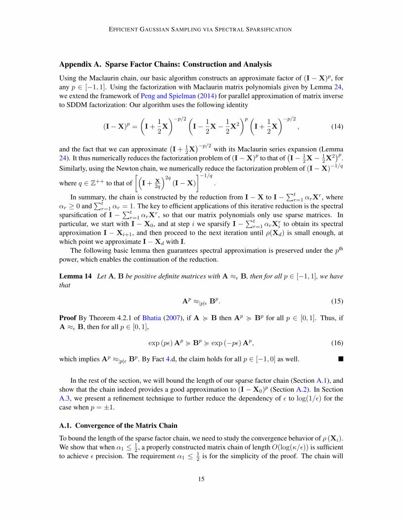
Appendix A. Sparse Factor Chains: Construction and Analysis

Using the Maclaurin chain, our basic algorithm constructs an approximate factor of (I −X)p, forany p ∈ [−1, 1]. Using the factorization with Maclaurin matrix polynomials given by Lemma 24,we extend the framework of Peng and Spielman (2014) for parallel approximation of matrix inverseto SDDM factorization: Our algorithm uses the following identity

(I−X)p =

(I +

1

2X

)−p/2(I− 1

2X− 1

2X2

)p(I +

1

2X

)−p/2, (14)

and the fact that we can approximate(I + 1

2X)−p/2 with its Maclaurin series expansion (Lemma

24). It thus numerically reduces the factorization problem of (I−X)p to that of(I− 1

2X− 12X2

)p.Similarly, using the Newton chain, we numerically reduce the factorization problem of (I−X)−1/q

where q ∈ Z++ to that of[(

I + X2q

)2q(I−X)

]−1/q.

In summary, the chain is constructed by the reduction from I −X to I −∑t

r=1 αrXr, where

αr ≥ 0 and∑t

r=1 αr = 1. The key to efficient applications of this iterative reduction is the spectralsparsification of I −

∑tr=1 αrX

r, so that our matrix polynomials only use sparse matrices. Inparticular, we start with I − X0, and at step i we sparsify I −

∑tr=1 αrX

ri to obtain its spectral

approximation I − Xi+1, and then proceed to the next iteration until ρ(Xd) is small enough, atwhich point we approximate I−Xd with I.

The following basic lemma then guarantees spectral approximation is preserved under the pth

power, which enables the continuation of the reduction.

Lemma 14 Let A, B be positive definite matrices with A ≈ε B, then for all p ∈ [−1, 1], we havethat

Ap ≈|p|ε Bp. (15)

Proof By Theorem 4.2.1 of Bhatia (2007), if A < B then Ap < Bp for all p ∈ [0, 1]. Thus, ifA ≈ε B, then for all p ∈ [0, 1],

exp (pε) Ap < Bp < exp (−pε) Ap, (16)

which implies Ap ≈|p|ε Bp. By Fact 4.d, the claim holds for all p ∈ [−1, 0] as well.

In the rest of the section, we will bound the length of our sparse factor chain (Section A.1), andshow that the chain indeed provides a good approximation to (I −X0)

p (Section A.2). In SectionA.3, we present a refinement technique to further reduce the dependency of ε to log(1/ε) for thecase when p = ±1.

A.1. Convergence of the Matrix Chain

To bound the length of the sparse factor chain, we need to study the convergence behavior of ρ (Xi).We show that when α1 ≤ 1

2 , a properly constructed matrix chain of length O(log(κ/ε)) is sufficientto achieve ε precision. The requirement α1 ≤ 1

2 is for the simplicity of the proof. The chain will

15


converge for any α1 such that 1 − α1 = Ω(1). Our analysis is analogous to the one in Peng andSpielman (2014). However, we have to deal with the general form, i.e., I−

∑tr=1 αrX

r.We define the following two polynomials for simplicity: fα(x) = 1 −

∑tr=1 αr (1− x)r and

gα(x) = 1 −∑bt/2c−1

r=0 αr (1− x)2r+1. For instance, the Maclaurin chain admits f(0.5,0.5)(x) =(3x− x2

)/2 and g(0.5,0.5)(x) = (3− x) /2.

We start with the following lemma, which analyzes one iteration of the chain construction. Wealso take into account the approximation error introduced by sparsification.

Lemma 15 Let X and X be nonnegative symmetric matrices such that I < X, I < X, and

I− X ≈ε I−t∑

r=1

αrXr. (17)

If ρ(X) ≤ 1−λ, then the eigenvalues of X all lie between 1−gα(λ) exp(ε) and 1−fα(λ) exp(−ε).

Proof If the eigenvalues of I−X are between λ and 2− λ, the eigenvalues of I−∑t

r=1 αrXr will

belong to [fα(λ), gα(λ)]. The bound stated in this lemma then follows from the fact that the spec-tral sparsification step preserves the eigenvalues of I−

∑tr=1 αrX

r to within a factor of exp(±ε).

We next prove that our Maclaurin chain achieves overall precision ε with length O(log(κ/ε)).

Lemma 16 (Short Maclaurin Chain) Let M = I−X0 be an SDDM matrix with condition num-ber κ. For any approximation parameter ε, there exists an (ε0, . . . , εd)-sparse factor chain of Mwith d = log9/8(κ/ε) and

∑dj=0 εj ≤ ε, satisfying

I−Xi+1 ≈εi I− 1

2Xi −

1

2X2i ∀ 0 ≤ i ≤ d− 1,

I−Xd ≈εd I.(18)

Proof Without loss of generality, we assume ε ≤ 110 . For 0 ≤ i ≤ d − 1, we set εi = ε

8d . Wewill show that our chain satisfies the condition given by Equation (18) with εd ≤ (7ε)/8, and thus∑d

i=0 εi ≤ ε.Let λi = 1−ρ(Xi). We split the error analysis to two parts, one for λi ≤ 1

2 , and one for λi ≥ 12 .

In the first part, because εi ≤ 1/10,

1− 1

2

(3λi − λ2i

)exp(−εi) < 1− 9

8λi and

1− 1

2(3− λi) exp(εi) > −1 +

9

8λi

(19)

which, by Lemma 15, implies that λi+1 ≥ 98λi. Because initially, λ0 ≥ 1/κ, after d1 = log9/8 κ

iterations, it must be the case that λd1 ≥ 12 . Now we enter the second part. Note that εi = ε

8d ≤ε6 .

Thus, when 12 ≤ λi ≤ 1− 5

6ε, we have εi ≤ 1−λi5 and therefore

1− 1

2

(3λi − λ2i

)exp(−εi) <

8

9(1− λi) and

1− 1

2(3− λi) exp(εi) >

8

9(−1 + λi)

(20)

16


which, by Lemma 15, implies that 1 − λi+1 ≤ 89(1 − λi). Because 1 − λd1 ≤ 1

2 , after anotherd2 = log9/8(1/ε) iterations, we get ρ (Xd1+d2) ≤ 5

6ε. Because exp(−78ε) < 1 − 5

6ε when ε < 110 ,

we conclude that (I−Xd1+d2) ≈εd I with εd ≤ 78ε.

Similarly, we can easily prove our Newton chain achieves overall precision εwith lengthO(log(κ/ε)).Indeed, any chain with α1 <

12 converges strictly faster than the Maclaurin chain.

Corollary 17 (Short Newton Chain) Let M = I−X0 be an SDDM matrix with condition num-ber κ and the vector α = (α1, α2, . . . , αt) with α1 ≤ 1

2 . For any approximation parameter ε,there exists an [(ε0, . . . , εd),α]-sparse factor chain of M with d = log9/8(κ/ε) and

∑dj=0 εj ≤ ε,

satisfying

I−Xi+1 ≈εi I−t∑

r=1

αrXr ∀ 0 ≤ i ≤ d− 1,

I−Xd ≈εd I.

(21)

A.2. Precision of the Factor Chain

We now bound the total error of the matrix factor that our algorithm constructs.

A.2.1. MACLAURIN CHAIN

We start with an error-analysis of a single reduction step in the algorithm.

Lemma 18 Fix p ∈ [−1, 1], given an ε-sparse factor chain, for all 0 ≤ i ≤ d − 1, there existsdegree ti polynomials, with ti = O(log(1/εi)), such that

(I−Xi)p ≈2εi T− 1

2p,ti

(I +

1

2Xi

)(I−Xi+1)

p T− 12p,ti

(I +

1

2Xi

). (22)

Proof

(I−Xi)p ≈εi T− 1

2p,ti

(I +

1

2Xi

)(I− 1

2Xi −

1

2X2i

)pT− 1

2p,ti

(I +

1

2Xi

)≈εi T− 1

2p,ti

(I +

1

2Xi

)(I−Xi+1)

p T− 12p,ti

(I +

1

2Xi

).

(23)

The first approximation follows from Lemma 24. The second approximation follows fromLemma 14, Fact 4.e, and I−Xi+1 ≈εi I− 1

2Xi − 12X2

i .

The next lemma bounds the total error of our construction.

Lemma 19 Define Zp,i as

Zp,i =

I if i = d, and(T− 1

2p,ti

(I + 1

2Xi

))Zp,i+1 if 0 ≤ i ≤ d− 1.

17


Then the following statement is true for all 0 ≤ i ≤ d

Zp,iZ>p,i ≈2

∑dj=i εj

(I−Xi)p . (24)

Proof We prove this lemma by reverse induction. Combine I ≈εd I−Xd and Lemma 14, we knowthat Zp,dZ

>p,d = Ip ≈εd (I−Xd)

p, so the claim is true for i = d. Now assume the claim is true fori = k + 1, then

Zp,kZ>p,k =T− 1

2p,tk

(I +

1

2Xk

)Zp,k+1Z

>p,k+1T− 1

2p,tk

(I +

1

2Xk

)≈2

∑dj=k+1 εj

T− 12p,tk

(I +

1

2Xk

)(I−Xk+1)

p T− 12p,tk

(I +

1

2Xk

)≈2εk (I−Xk)

p .

(25)

The last approximation follows from Lemma 18.

If we define C to be Z− 12,0, this lemma implies CC> ≈2

∑dj=0 εj

(I−X0)−1.

A.2.2. NEWTON CHAIN

We start with an error-analysis of a single reduction step in the algorithm. We assume that the2q + 1-dimensional vector α, where q ∈ Z++, is defined by the identity: 1 −

∑2q+1r=1 αr =(

1 + x2q

)2q(1− x).

Lemma 20 Fix p ∈ [−1, 1], given an ε-sparse factor chain, for all 0 ≤ i ≤ d − 1, there existsdegree ti polynomials, with ti = O(log(1/εi)), such that

(I−Xi)−1/q ≈εi

(I +

Xi

2q

)(I−Xi+1)

−1/q(

I +Xi

2q

). (26)

Proof

(I−Xi)−1/q =

(I +

Xi

2q

)(I−

2q+1∑r=1

αrXri

)−1/q (I +

Xi

2q

)≈εi

(I +

Xi

2q

)(I−Xi+1)

−1/q(

I +Xi

2q

).

(27)

The first identity follows from Equation 10. The second approximation follows from Lemma14, Fact 4.e, and I−Xi+1 ≈εi I−

∑2q+1r=1 αrX

ri .

The next lemma bounds the total error of our construction.

Lemma 21 Define Wq,i as

Wq,i =

I if i = d, and(I + Xi

2q

)Wq,i+1 if 0 ≤ i ≤ d− 1.

18


Then the following statement is true for all 0 ≤ i ≤ d

Wq,iW>q,i ≈∑d

j=i εj(I−Xi)

−1/q . (28)

Proof The proof is similar to Lemma 19.

If we define C to be W1,0, this lemma implies CC> ≈∑dj=0 εj

(I−X0)−1.

A.3. Iterative Refinement for Inverse Square-Root Factor

In this section, we provide a highly accurate factor for the case when p = −1. We use a refinementapproach inspired by the precondition technique for square factors described in Section 2.2 of Chowand Saad (2014).

Theorem 22 For any symmetric positive definite matrix M, any matrix C such that M−1 ≈O(1)

ZZ>, and any error tolerance ε > 0, there exists a linear operator C which is an O(log(1/ε))-degree polynomial of M and Z, such that CC> ≈ε M−1.

ProofStarting from M−1 ≈O(1) ZZ>, we know that Z>MZ ≈O(1) I. This implies that κ(Z>MZ) =

O(1), which we can scale Z>MZ so that its eigenvalues lie in [1 − δ, 1 + δ] for some constant0 < δ < 1.

By applying Lemma 23 on its eigenvalues, there is an O(log(1/ε)) degree polynomial T− 12,t(·)

that approximates the inverse square root of Z>MZ, i.e.(T− 1

2,O(log(1/ε))

(Z>MZ

))2≈ε(Z>MZ

)−1. (29)

Here, we can rescale Z>MZ back inside T− 12,t(·), which does not affect the multiplicative error.

Then by Fact 4.e, we have

Z(T− 1

2,O(log(1/ε))

(Z>MZ

))2Z> ≈ε Z

(Z>MZ

)−1Z> = M−1. (30)

So if we define the linear operator C = Z(T− 1

2,O(log(1/ε))

(Z>MZ

)), C satisfies the claimed

properties.

Note that this refinement procedure is specific to p = ±1. It remains open if it can be extended togeneral p ∈ [−1, 1].

Appendix B. Maclaurin Series Expansion

We show how to approximate(I + 1

2X)p, when ρ (X) < 1. Because I + 1

2X is well-conditioned,we can approximate its pth power to any approximation parameter ε > 0 using anO(log(1/ε))-orderMaclaurin expansion, i.e., a low degree polynomial of X. Moreover, since the approximation is apolynomial of X, the eigenbasis is preserved. We start with the following lemma on the residue ofMaclaurin expansion.

19


Lemma 23 (Maclaurin Series) Fix p ∈ [−1, 1] and δ ∈ (0, 1), for any error tolerance ε > 0,there exists a t-degree polynomial Tp,t(·) with t ≤ log(1/(ε(1−δ)2)

1−δ , such that for all λ ∈ [1−δ, 1+δ],

exp(−ε)λp ≤ Tp,t(λ) ≤ exp(ε)λp. (31)

Proof Let gp,t (x) =∑∞

i=0 aixi be the tth order Maclaurin series expansion of (1− x)p. Because

|a1| = |p| ≤ 1, and |ak+1| =∣∣∣p−kk+1

∣∣∣ |ak| ≤ |ak|, we can prove that |ai| ≤ 1 for all i by induction.For |x| ≤ δ < 1, we have

|(1− x)p − gp,t (x)| =

∣∣∣∣∣∞∑

i=t+1

aixi

∣∣∣∣∣ ≤∞∑

i=t+1

δi =δt+1

1− δ. (32)

We define Tp,t (x) = gp,t (1− x). Because |1− λ| ≤ δ and λp ≥ 1− δ,

|Tp,t (λ)− λp| ≤ δt+1

1− δ≤ δt+1

(1− δ)2λp. (33)

Therefore, when t = (1− δ)−1 log(1/(ε(1− δ)2))), we get δt+1

(1−δ)2 < ε and

|Tp,t (λ)− λp| ≤ ελp, (34)

which implies

exp(−ε)λp ≤ Tp,t (λ) ≤ exp(ε)λp. (35)

Now we present one of our key lemmas, which provides the backbone for bounding overall errorof our sparse factor chain. We claim that substituting

(I + 1

2X)p with its Maclaurin expansion into

Equation 7 preserves the multiplicative approximation. We prove the lemma for p ∈ [−1, 1] whichlater we use for computing the pth power of SDDM matrices. For computing the inverse square-rootfactor, we only need the special case when p = −1.

Lemma 24 (Factorization with Matrix Polynomials) Let X be a symmetric matrix with ρ (X) <1 and fix p ∈ [−1, 1]. For any approximation parameter ε > 0, there exists a t-degree polynomialTp,t(·) with t = O(log(1/ε)), such that

(I−X)p ≈ε T− p2,t

(I +

1

2X

)(I− 1

2X− 1

2X2

)pT− p

2,t

(I +

1

2X

). (36)

Proof Take the spectral decomposition of X

X =∑i

λiuiu>i , (37)

20


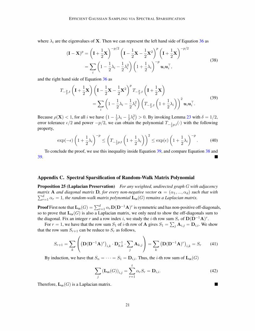
where λi are the eigenvalues of X. Then we can represent the left hand side of Equation 36 as

(I−X)p =

(I +

1

2X

)−p/2(I− 1

2X− 1

2X2

)p(I +

1

2X

)−p/2=∑i

(1− 1

2λi −

1

2λ2i

)(1 +

1

2λi

)−puiu

>i ,

(38)

and the right hand side of Equation 36 as

T− p2,t

(I +

1

2X

)(I− 1

2X− 1

2X2

)pT− p

2,t

(I +

1

2X

)=∑i

(1− 1

2λi −

1

2λ2i

)(T− p

2,t

(1 +

1

2λi

))2

uiu>i .

(39)

Because ρ(X) < 1, for all i we have(1− 1

2λi −12λ

2i

)> 0. By invoking Lemma 23 with δ = 1/2,

error tolerance ε/2 and power −p/2, we can obtain the polynomial T− 12p,t(·) with the following

property,

exp(−ε)(

1 +1

2λi

)−p≤(T− 1

2p,t

(1 +

1

2λi

))2

≤ exp(ε)

(1 +

1

2λi

)−p. (40)

To conclude the proof, we use this inequality inside Equation 39, and compare Equation 38 and39.

Appendix C. Spectral Sparsification of Random-Walk Matrix Polynomial

Proposition 25 (Laplacian Preservation) For any weighted, undirected graph G with adjacencymatrix A and diagonal matrix D, for every non-negative vector α = (α1, ..., αd) such that with∑d

r=1 αr = 1, the random-walk matrix polynomial Lα(G) remains a Laplacian matrix.

Proof First note that Lα(G) =∑d

r=1 αrD(D−1A)r is symmetric and has non-positive off-diagonals,so to prove that Lα(G) is also a Laplacian matrix, we only need to show the off-diagonals sum tothe diagonal. Fix an integer r and a row index i, we study the i-th row sum Sr of D(D−1A)r.

For r = 1, we have that the row sum S1 of i-th row of A gives S1 =∑

j Ai,j = Di,i. We showthat the row sum Sr+1 can be reduce to Sr as follows,

Sr+1 =∑k

(D(D−1A)r)i,k·D−1k,k ·

∑j

Ak,j

=∑k

(D(D−1A)r

)i,k

= Sr (41)

By induction, we have that Sn = · · · = S1 = Di,i. Thus, the i-th row sum of Lα(G)

∑j

(Lα(G))i,j =t∑

r=1

αrSr = Di,i. (42)

Therefore, Lα(G) is a Laplacian matrix.

21


Lemma 26 (Two-Step Supports) For a graph Laplacian matrix L = D−A, with diagonal matrixD and nonnegative off-diagonal A, for all positive odd integer r, we have

1

2LG LGr rLG. (43)

and for all positive even integers r we have

LG2 LGr r

2LG2 . (44)

Proof Let X = D−12 AD−

12 , for any integer r, the statements are equivalent to

1

2(I−X) I−X2r+1 (2r + 1) (I−X) (45)

I−X2 I−X2r r(I−X2

). (46)

Because X can be diagonalized by unitary matrix U as Λ = UXU>, where Λ = diag(λ1, λ2, . . . , λn)and λi ∈ [−1, 1] for all i. Therefore we can reduce the inequalities to the scalar case, and we con-clude the proof with the following inequalities:

1

2(1− λ) ≤ 1− λ2r+1 ≤ (2r + 1) (1− λ), ∀λ ∈ (−1, 1) and odd integer r;

(1− λ2) ≤ 1− λ2r ≤ r(1− λ2), ∀λ ∈ (−1, 1) and even integer r.(47)

Lemma 27 (Upper Bounds on Effective Resistance) For a graph G with Laplacian matrix L =D−A, let LGr = D−D(D−1A)r be its r-step random-walk matrix. Then, the effective resistancebetween two vertices u0 and ur on LGr is upper bounded byRGr(u0, ur) ≤

∑ri=1

2A(ui−1,ui)

, where(u0 . . . ur) is a path in G.

Proof When r is a positive odd integer, by Lemma 26, we have that 12LG LGr , which implies

that for any edge (u, v) in G,

RGr(u, v) ≤ 2rG(u, v) =2

A(u, v). (48)

Because effective resistance satisfies triangular inequality, this concludes the proof for odd r.When r is even, by Lemma 26, we have that LG2 LGr . The effective resistance of D −

AD−1A is studied in Peng and Spielman (2014) and restated in Proposition 28. For the subgraphG2(u) anchored at the vertex u (the subgraph formed by length-2 paths where the middle node isu), for any two of its neighbors v1 and v2, we have

RGr(v1, v2) ≤ RG2(u)(v1, v2) =1

A(v1, u)+

1

A(u, v2). (49)

Because we have the above upper bound for any 2-hop path (v1, u, v2), by the triangular inequalityof effective resistance, the lemma holds for even r as well.

22


Proposition 28 (Claim 6.3. from Peng and Spielman (2014)) Given a graph of size n with theLaplacian matrix L = D− 1

daa>, where Di,i = (ais)/dwith s =

∑ni=1 ai. The effective resistance

for edge (i, j) is

d

s(

1

ai+

1

aj). (50)

Proof Let ei denote the vector where the i-th entry is 1, and 0 everywhere else. We have

dL

(eiai− ejaj

)= (s− ai)ei −

∑k 6=i

akek − (s− aj)ej +∑k 6=j

akek = s(ei − ej). (51)

Therefore

(ei − ej)>L†(ei − ej) =d

s(ei − ej)>(

eiai− ejaj

) =d

s(

1

ai+

1

aj). (52)

Lemma 29 (A Random-Walk Identity) Given a graphGwithm edges, consider the r-step random-walk graph Gr and the corresponding Laplacian matrix LGr = D −D(D−1A)r. For a length-rpath p = (u0 . . . ur) on G, we have

w(p) =

∏ri=1 A(ui−1, ui)∏r−1i=1 D(ui, ui)

, Z(p) =

r∑i=1

2

A(ui−1, ui).

The summation of w(p)Z(p) over all length-r paths satisfies∑p

w(p) · Z(p) = 2rm. (53)

Proof We substitute the expression for w(p) and Z(p) in to the summation.∑p=(u0...ur)

w(p)Z(p) =∑p

(r∑i=1

2

A(ui−1, ui)

)(∏rj=1 A(uj−1, uj)∏r−1j=1 D(uj , uj)

)(54)

= 2∑p

r∑i=1

(∏i−1j=1 A(uj−1, uj)

∏r−1j=i A(uj , uj+1)∏r−1

j=1 D(uj , uj)

)(55)

= 2∑e∈G

r∑i=1

∑p with (ui−1,ui)=e

∏i−1j=1 A(uj−1, uj)

∏r−1j=i A(uj , uj+1)∏r−1

j=1 D(uj , uj)

(56)

= 2∑e∈G

r∑i=1

∑p with (ui−1,ui)=e

∏i−1j=1 A(uj−1, uj)∏i−1j=1 D(uj , uj)

·∏r−1j=i A(uj , uj+1)∏r−1j=i D(uj , uj)

(57)

= 2∑e∈G

r∑i=1

1 (58)

= 2mr. (59)

23


From Equation 55 to 56, instead of enumerating all paths, we first fix an edge e to be the i-thedge on the path, and then extend from both ends of e. From Equation 57 to 58, we sum over indicesiteratively from u0 to ui−1, and from ur to ui. Because D(u, u) =

∑v A(u, v), this summation

over all possible paths anchored at (ui−1, ui) equals to 1.

When computing the qth root, the work of chain construction depends quadratically on q, whilethe multiplication with vector cost the same for all q. Thus it should be only used for q = O(1).

Theorem 30 (Factoring M−1/q) For any q ∈ Z+, and an SDDM matrix M = I − X0, we canconstruct a representation of an n×nmatrix C such that CC> ≈ε M−1/q in workO(m·q2·logc1 n·logc2(κ/ε)/ε4) and depth O(q · logc3 n · log(κ/ε)) for some constants c1, c2, and c3. Moreover, forany x ∈ Rn, we can compute Cx in work O(m + n · logc n · log3(κ/ε)/ε2) and depth O(log n ·log(κ/ε)) for some other constant c.

Appendix D. Extension to SDDM Matrices

Our path sampling algorithm from Section 5 can be generalized to an SDDM matrix with splittingD −A. The idea is to split out the extra diagonal entries to reduce it back to the Laplacian case.Of course, the D−1 in the middle of the monomial is changed, however, it only decreases the trueeffective resistance so the upper bound in Lemma 10 still holds without change. The main differenceis that we need to put back the extra diagonal entries, which is done by multiplying an all 1 vectorthrough D−D(D−1A)r.

The follow Lemma can be proved similar to Lemma 25.

Lemma 31 (SDDM Preservation) If M = D − A is an SDDM matrix with diagonal matrixD and nonnegative off-diagonal A, for any nonnegative α = (α1, . . . , αd) with

∑dr=1 αr = 1,

Mα = D−∑d

r=1 αrD(D−1A)r is also an SDDM matrix.

Our algorithm is a direction modification of the algorithm from Section 5. To analyze it, weneed a variant of Lemma 10 that bounds errors w.r.t. the matrix by which we measure effectiveresistances. We use the following statement from Peng (2013).

Lemma 32 (Lemma B.0.1. from Peng (2013)) Let A =∑

i yTe ye and B be n× n positive semi-

definite matrices such that the image space of A is contained in the image space of B, and τ be aset of estimates such that

τe ≥ yTe B†ye ∀e.Then for any error ε and any failure probability δ = n−d, there exists a constant cs such that if weconstruct A using the sampling process from Figure 1, with probability at least 1 − δ = 1 − n−d,A satisfies:

A− ε (A + B) A A + ε (A + B) .

Theorem 33 (SDDM Polynomials Sparsification) Let M = D−A be an SDDM matrix with di-agonal D, nonnegative off-diagonal A withm nonzero entries, for any nonnegativeα = (α1, . . . , αd)with

∑dr=1 αr = 1, we can define Mα = D −

∑dr=1 αrD(D−1A)r. For any approximation pa-

rameter ε > 0, we can construct an SDDM matrix M with O(n log n/ε2) nonzero entries, in timeO(m · log2 n · d2/ε2), such that M ≈ε Mα.

24


ProofWe look at each monomial separately. First, by Lemma 31, Mr is an SDDM matrix. It can

be decomposed as the sum of two matrices, a Laplacian matrix Lr = Dr −D(D−1A)r, and theremaining diagonal Dextra. As in the Laplacian case, a length-r paths in D −A corresponds to anedge in Lr. We apply Lemma 32 to Mr and Lr =

∑e∈P yey

>e , where P is the set of all length-r

paths in D−A, and ye is the column of the incidence matrix associated with e.When r is an odd integer, we have

y>e (Mr)−1 ye ≤ 2y>e (D−A)−1 ye, (60)

and when r is an even integer, we have

y>e (Mr)−1 ye ≤ 2y>e

(D−AD−1A

)−1ye. (61)

Let e denote the edge corresponds to the length-r path (u0, . . . , ur), the weight of e is

w(e) = w(u0 . . . ur) = y>e ye =

∏ri=1 A(ui−1, ui)∏r−1i=1 D(ui, ui)

≤∏ri=1 A(ui−1, ui)∏r−1i=1 Dg(ui, ui)

, (62)

where Dg(u, u) =∑

v 6=u A(u, v), so we have the same upper bound as the Laplacian case, and wecan sample random walks in the exact same distribution.

By Lemma 32 there exists M = O(r ·m · log n/ε2) such that with probability at least 1 − 1n ,

the sampled graph G = GRAPHSAMPLING(Gr, τe,M) satisfies

Mr −1

2ε(Lr + Mr) 4 LG + Dextra 4 Mr +

1

2ε(Lr + Mr). (63)

Now if we set M = LG + Dextra, we will have

(1− ε)Mr 4 M 4 (1 + ε)Mr. (64)

Note that Dextra can be computed efficiently by computing diag(Mr1) via matrix-vector multipli-cations.

Appendix E. Gremban’s Reduction for Inverse Square Root Factor

We first note that Gremban’s reduction (Gremban, 1996) can be extended from solving linear sys-tems to computing the inverse square-root factor. The problem of finding a inverse factor of an SDDmatrix, can be reduced to finding a inverse factor of an SDDM matrix that is twice as large.

Lemma 34 Let Λ = D + An + Ap be an n× n SDD matrix, where D is the diagonal of Λ, Ap

contains all the positive off-diagonal entries of Λ, and An contains all the negative off-diagonalentries.

Consider the following SDDM matrix S, and an inverse factor C of S, such that

S =

[D + An −Ap

−Ap D + An

]and CC> = S. (65)

25


Let In be the n× n identity matrix. The matrix

C =1√2

[In −In

]C

is an inverse square-root factor of Λ.

Proof We can prove that

Λ−1 =1

2

[In −In

]S−1

[In−In

](66)

thus we have CC> = Λ−1.

Note that if C is 2n × 2n, C will be an n × 2n matrix. Given the non-square inverse factorC, we can draw a sample from multivariate Gaussian distribution with covariance Λ−1 as follows.First draw 2n i.i.d. standard Gaussian random variables x = (x1, x2, . . . , x2n)>, then y = Cx is amultivariate Gaussian random vector with covariance Λ−1.

Appendix F. Commutative Splitting of SDDM Matrices

For an SDDM matrix D−A, one way to normalize it is to multiply D−1/2 on both sides,

D−A = D1/2(I−D−1/2AD−1/2

)D1/2.

Because ρ(D−1/2AD−1/2

)< 1, this enables us to approximate

(I−D−1/2AD−1/2

)p. It is not

clear how to undo the normalization and obtain (D−A)p from it, due to the fact that D and A donot commute. Instead, we consider another normalization as in Lemma 3 and provide its proof.

Lemma 35 (Commutative Splitting) For an SDDM matrix M = D − A with diagonal D =diag (d1, d2, . . . , dn), and let κ = max2, κ (D−A). We can pick c = (1− 1/κ) /(maxi di), sothat all eigenvalues of c (D−A) lie between 1

2κ and 2− 12κ . Moreover, we can rewrite c (D−A)

as an SDDM matrix I−X, where all entries of X = I− c (D−A) are nonnegative, and ρ (X) ≤1− 1

2κ .

Proof Let j = arg maxi di, by definition c = (1− 1/κ) /dj .Let [λmin, λmax] denote the range of the eigenvalues of D − A. By Gershgorin circle the-

orem and the fact that D − A is diagonally dominant, we have that λmax ≤ 2dj . Also dj =e>j (D−A) ej , so λmax ≥ dj , and therefore λmin ≥ λmax/κ ≥ dj/κ.

The eigenvalues of c (D−A) lie in the interval [cλmin, cλmax], and can be bounded as

1

2κ≤(

1− 1

κ

)1

dj

(djκ

)≤ cλmin ≤ cλmax ≤

(1− 1

κ

)1

dj(2dj) ≤ 2− 1

2κ. (67)

To see that X = (I− cD) + cA is a nonnegative matrix, note that A is nonnegative and I is entry-wise larger than cD.

26


Appendix G. Inverse Factor by Combinatorial SDDM Factorization

A simple combinatorial construction of C follows from the fact that SDDM matrices can be factor-ized.

Lemma 36 (Combinatorial Factorization) Let M be an SDDM matrix with m non-zero entriesand condition number κ, then

(1) M can be factored intoM = BB>,

where B is an n×m matrix with at most 2 non-zeros per column;

(2) for any approximation parameter ε > 0, if Z is linear operator satisfying Z ≈ε M−1, thenthe matrix

C = ZB

satisfiesCC> ≈2ε M−1.

Moreover, a representation of C can be computed in work O(m · logc1 n · logc2 κ) and depthO(logc3 n · log κ) for some modest constants c1, c2, and c3 so that for any m-dimensionalvector x, the product Cx can be computed in work O((m + n · logc n · log3 κ) · log(1/ε))and depth O(log n · log κ · log(1/ε)) for a modest constant c.

Proof Let ei be the ith standard basis, then M can be represented by

M =1

2

∑1≤i<j≤n

|Mi,j | (ei − ej) (ei − ej)> +

n∑i=1

aieie>i ,

where ai = Mi,j −∑

j 6=i |Mi,j | ≥ 0. Indeed, we can rewrite M as∑m

i=1 yiy>i this way, and by

setting B = (y1,y2, . . . ,ym) concludes the proof for statement (1).For statement (2),

CC> = ZBB>Z>

= ZMZ

≈ε ZZ−1Z = Z.

(68)

The third line is true because of Fact 4.d and Fact 4.e. From CC> ≈ε Z, by Fact 4.c, we haveCC> ≈2ε M−1.

The total work and depth of constructing the operator ZB is dominated by the work and depthof constructing the approximate inverse Z, which we refer to the analysis in Peng and Spielman(2014). The same statement also holds for the work and depth of matrix-vector multiplication ofZB.

In particular, the parallel solver algorithm from Peng and Spielman (2014) computes Z ≈ε M−1

in total work nearly-linear in m, and depth polylogarithmic in n, κ and ε−1. However, it requires mi.i.d. standard Gaussian samples to generate an n-dimensional Gaussian random vector.

27

Efﬁcient Sampling for Gaussian Graphical … Workshop and Conference Proceedings vol 40:1–27,...

Documents

Transcript of Efﬁcient Sampling for Gaussian Graphical … Workshop and Conference Proceedings vol 40:1–27,...