Efficient nonlinear manifold reduced order model

Youngkyu KimMechanical Engineering

University of California, BerkeleyBerkeley, CA 94720

youngkyu_kim@berkeley.edu

Youngsoo ChoiCenter for Applied Scientific ComputingLawrence Livermore National Laboratory

Livermore, CA 94550choi15@llnl.gov

David WidemannComputational Engineering Division

Lawrence Livermore National LaboratoryLivermore, CA 94550widemann1@llnl.gov

Tarek ZohdiMechanical Engineering

University of California, BerkeleyBerkeley, CA 94720

zohdi@berkeley.edu

Abstract

Traditional linear subspace reduced order models (LS-ROMs) are able to acceleratephysical simulations, in which the intrinsic solution space falls into a subspacewith a small dimension, i.e., the solution space has a small Kolmogorov n-width.However, for physical phenomena not of this type, such as advection-dominatedflow phenomena, a low-dimensional linear subspace poorly approximates thesolution. To address cases such as these, we have developed an efficient nonlinearmanifold ROM (NM-ROM), which can better approximate high-fidelity modelsolutions with a smaller latent space dimension than the LS-ROMs. Our methodtakes advantage of the existing numerical methods that are used to solve thecorresponding full order models (FOMs). The efficiency is achieved by developinga hyper-reduction technique in the context of the NM-ROM. Numerical resultsshow that neural networks can learn a more efficient latent space representationon advection-dominated data from 2D Burgers’ equations with a high Reynoldsnumber. A speed-up of up to 11.7 for 2D Burgers’ equations is achieved with anappropriate treatment of the nonlinear terms through a hyper-reduction technique.

1 Introduction

Physical simulations are influencing developments in science, engineering, and technology morerapidly than ever before. However, high-fidelity, forward physical simulations are computationallyexpensive and, thus, make intractable many decision-making applications, such as design optimization,inverse problems, optimal controls, and uncertainty quantification. These applications require manyforward simulations to explore the parameter space in the outer loop. To compensate for thecomputational expense issue, many surrogate models have been developed: from simply usinginterpolation schemes for specific quantity of interests to physics-informed surrogate models. Thispaper focuses on the latter because a physics-informed surrogate model is more robust in predictingphysical solutions than the simple interpolation schemes.

Among many types of physics-informed surrogate models, the projection-based linear subspacereduced order models (LS-ROMs) take advantage of both the known governing equation and datawith linear subspace solution representation [1]. Although LS-ROMs have been successfully appliedto many forward physical problems [2–10] and partial differential equation(PDE)-constrained opti-mization problems [11–14], the linear subspace solution representation suffers from not being ableto represent certain physical simulation solutions with a small basis dimension, such as advection-

Workshop on machine learning for engineering modeling, simulation and design @ NeurIPS 2020

dominated or sharp gradient solutions. This is because LS-ROMs work only for physical problems,in which the intrinsic solution space falls into a subspace with a small dimension, i.e., the solutionspace has a small Kolmogorov n-width. Although there have been many attempts to resolve theseshortcomings of LS-ROMs with various methods, [15–29], all these approaches are still based on thelinear subspace solution representation. We transition to a nonlinear, low-dimensional manifold toapproximate the solution better than linear methods.

There are many works available in the current literature that looked into the nonlinear manifoldsolution represenation, using neural networks (NNs) as surrogates for physical simulations [30–48].However, these methods do not take advantage of the existing numerical methods for high-fidelityphysical simulations. Recently, a neural network-based ROM is developed in [49], where the weightsand biases are determined in the training phase and the existing numerical methods are utilized intheir models. The same technique is extended to preserve the conserved quantities in the physicalconservation laws [50]. However, their approaches do not achieve any speed-up because the nonlinearterms that still scale with the corresponding FOM size need to be updated every time step or Newtonstep.

We present a fast and accurate physics-informed neural network ROM with a nonlinear manifoldsolution representation, i.e., the nonlinear manifold ROM (NM-ROM). We train a shallow maskedautoencoder with solution data from the corresponding FOM simulations and use the decoder asthe nonlinear manifold solution representation. Our NM-ROM is different from the aformentionedphysics-informed neural networks in that we take advantage of the existing numerical methods ofsolving PDE in our approach and a considerable speed-up is achieved.

2 Full order model

A parameterized nonlinear dynamical system is considered, characterized by a system of nonlinearordinary differential equations (ODEs), which can be considered as a resultant system from semi-discretization of Partial Differential Equations (PDEs) in space domains

dx

dt= f(x, t;µ), x(0;µ) = x0(µ), (1)

where t ∈ [0, T ] denotes time with the final time T ∈ R+, and x(t;µ) denotes the time-dependent,parameterized state implicitly defined as the solution to problem (1) with x : [0, T ] × D → RNs .Further, f : RNs × [0, T ] × D → RNs with (w, τ ;ν) 7→ f(w, τ ;ν) denotes the time derivativeof x, which we assume to be nonlinear in at least its first argument. The initial state is denoted byx0 : D → RNs , and µ ∈ D denotes parameters in the domain D ⊆ Rnµ .

A uniform time discretization is assumed throughout the paper, characterized by time step ∆t ∈ R+

and time instances tn = tn−1 + ∆t for n ∈ N(Nt) with t0 = 0, Nt ∈ N, and N(N) := 1, . . . , N.To avoid notational clutter, we introduce the following time discretization-related notations: xn :=x(tn;µ), xn := x(tn;µ), xn := x(tn;µ), and fn := f(x(tn;µ), tn;µ), where x, x, x and f aredefined in. The implicit backward Euler (BE)1 time integrator numerically solves Eq. (1), by solvingthe following nonlinear system of equations, i.e., xn − xn−1 = ∆tfn, for xn at n-th time step. Thecorresponding residual function is defined as

rnBE(xn;xn−1,µ) := xn − xn−1 −∆tfn. (2)

3 Nonlinear manifold reduced order model (NM-ROM)

The NM-ROM applies solution representation using a nonlinear manifold S := g (v) |v ∈ Rns,where g : Rns → RNs with ns Ns denotes a nonlinear function that maps a latent space ofdimension ns to the full order model space of dimension, Ns. That is, the NM-ROM approximatesthe solution in a trial manifold as

x ≈ x = xref + g (x) . (3)

1Other time integrators can be used in our NM-ROMs.

2

The construction of the nonlinear function, g, is explained in Section 4. By plugging Eq. (3) intoEq. (2), the residual function at nth time step becomes

rnBE(xn; xn−1,µ) := rnBE(xref + g (xn) ;xref + g (xn−1) ,µ)

= g (xn)− g (xn−1)−∆tf(xref + g (xn) , tn;µ),(4)

which is an over-determined system that we close with the least-squares Petrov–Galerkin (LSPG)projection. That is, we minimize the squared norm of the residual vector function at every time step:

xn = argminv∈Rns

1

2‖rnBE(v; xn−1,µ)‖22 . (5)

The Gauss–Newton method with the starting point xn−1 is applied to solve the minimizationproblem (5). However, the nonlinear residual vector, rnBE, scales with FOM size and it needs to beupdated every time the argument of the function changes, which occurs either at every time stepor Gauss–Newton step. More specifically, if the backward Euler time integrator is used, g (xn),f(xref + g (xn) , t;µ), and their Jacobians need to be updated whenever xn changes. Without anyspecial treatment on the nonlinear residual term, no speed-up can be expected. Thus, we apply ahyper-reduction to eliminate the scale with FOM size in the nonlinear term evaluations (see Section 5).Finally, we denote this non-hyper-reduced NM-ROM as NM-LSPG.

4 Shallow masked autoencoder

The nonlinear function, g, is the decoderD of an autoencoder in the form of a feedforward neuralnetwork. The autoencoder compresses FOM solutions of Eq. (1) with an encoderE and decompressesback to reconstructed FOM solution with an decoderD. The autoencoder is trained to reconstruct theFOM solutions of Eq. (1) by minimizing the mean square error between original and reconstructedFOM solutions. Therefore, the dimension of the encoder input and the decoder output is Ns and thedimension of the encoder E output and the decoderD input is ns.

We intentionally use a non-deep neural network, i.e., three-layer autoencoder, for the decoder toachieve an efficiency that is requried by the hyper-reduction (see Section 5). More specifically, thefirst layers of the encoderE and decoderD are fully-connected layers, where the nonlinear activationfunctions are applied and the last layer of the encoder E is fully-connected layer with no activationfunctions. The last layer of the decoderD is sparsely-connected layer with no activation functions.The sparsity is determined by a mask matrix. These network architectures are shown in Fig. 1.

(a) Without masking (b) With masking

Figure 1: Three-layer encoder/decoder architectures: (a) unmasked and (b) after the sparsity maskis applied. Nodes and edges in orange color represent active path in the subnet that stems from thesampled outputs that are marked as the orange disks. Note that the masked shallow neural networkhas a sparser structure than the unmasked one. A sparser structure leads to a more efficient model.

There is no way to determine hidden layer sizes a priori. If the number of learnable parameters isnot enough, the decoder is not able to represent the nonlinear manifold well. On the other hand,

3

too many learnable parameters may result in over-fitting, so the decoder is not able to generalizewell, which means the trained decoder cannot be used for problems whose data is unseen, i.e., thepredictive case. To avoid over-fitting, we first divide the training data into train and validation datasets.Then, the autoencoder is trained using the train dataset and tested for the generalization using thevalidation dataset. If the mean squared errors on the validation and train datasets are very different,then over-fitting has occurred. We then reduce the size of the hidden layer and re-train the model[51].

5 Hyper-reduction

The hyper-reduction techniques are developed to eliminate the FOM scale dependecy in nonlinearterms [52–54, 17, 19], which is essential to acheive an efficiency in our NM-ROM. We follow thegappy POD approach [55], in which the nonlinear residual term is approximated as

r ≈ Φrr, (6)

where Φr := [φr,1, . . . ,φr,nr ] ∈ RNs×nr , ns ≤ nr Ns, denotes the residual basis matrix andr ∈ Rnr denotes the generalized coordinates of the nonlinear residual term. Here, r representsa residual vector function, e.g., the backward Euler residual, rnBE , defined in Eq. (4). We usethe singular value decomposition of the FOM solution snapshot matrix to construct Φr, which isjustified in [19]. In order to find r, we apply a sampling matrix ZT := [ep1 , . . . , epnz ]T ∈ Rnz×Ns ,ns ≤ nr ≤ nz Ns on both sides of (6). The vector, epi , is the pith column of the identity matrixINs ∈ RNs×Ns . Then the following least-squares problem is solved:

r := argminv∈Rnr

1

2

∥∥∥ZT (r −Φrv)∥∥∥22. (7)

The solution to Eq. (7) is given as r = (ZTΦr)†ZT r, where the Moore–Penrose inverse of a matrixA ∈ Rnz×nr with full column rank is defined asA† := (ATA)−1AT . Therefore, Eq. (6) becomesr ≈ P r, where P := Φr(ZTΦr)†ZT is the oblique projection matrix. We do not construct thesampling matrix Z. Instead, it maintains the sampling indices p1, . . . , pnf and correspondingrows of Φr and r. This enables hyper-reduced ROMs to achieve a speed-up. The sampling indices(i.e., Z) can be determined by Algorithm 3 of [17] for computational fluid dynamics problems andAlgorithm 5 of [56] for other problems.

The hyper-reduced residual, P rnBE , is used in the minimization problem in Eq. (5):

xn = argminv∈Rns

1

2

∥∥∥ (ZTΦr)†ZT rnBE(v; xn−1,µ)∥∥∥22. (8)

Note that the pseudo-inverse (ZTΦr)† can be pre-computed. Due to the definition of rnBE in Eq. (4),the sampling matrix Z needs to be applied to the following two terms: g (xn) − g (xn−1) andf(xref + g (xn) , t;µ) at every time step. The first term, ZT (g (xn) − g (xn−1)), requires thatonly selected outputs of the decoder be computed. Furthermore, for the second term, the nonlinearresidual elements that are selected by the sampling matrix need to be computed. This implies thatwe have to keep track of the outputs of g that are needed to compute the selected nonlinear residualelements by the sampling matrix, which is usually a larger set than the outputs that are selected solelyby the sampling matrix. Therefore, we build a subnet that computes only the outputs of the decoderthat are required to compute the nonlinear residual elements. Such outputs are demonstrated as thesolid oragne disks and the corresponding subnet is depicted in Fig. 1(b). Finally, we denote thishyper-reduced NM-ROM as NM-LSPG-HR.

6 2D Burgers’ equation

We demonstrate the performance of our NM-ROMs (i.e., NM-LSPG and NM-LSPG-HR) by compar-ing it with LS-ROMs (i.e., LS-LSPG and LS-LSPG-HR) that was first introduced in [56]. We solve

4

the following parameterized 2D viscous Burgers’ equation:

∂u

∂t+ u

∂u

∂x+ v

∂u

∂y=

1

Re

(∂2u

∂x2+∂2u

∂y2

)∂v

∂t+ u

∂v

∂x+ v

∂v

∂y=

1

Re

(∂2v

∂x2+∂2v

∂y2

)(x, y) ∈ Ω = [0, 1]× [0, 1]

t ∈ [0, 2],

(9)

with the boundary condition

u(x, y, t;µ) = v(x, y, t;µ) = 0 on Γ = (x, y)|x ∈ 0, 1, y ∈ 0, 1 (10)

and the initial condition

u(x, y, 0;µ) =

µ sin (2πx) · sin (2πy) if (x, y) ∈ [0, 0.5]× [0, 0.5]0 otherwise (11)

v(x, y, 0;µ) =

µ sin (2πx) · sin (2πy) if (x, y) ∈ [0, 0.5]× [0, 0.5]0 otherwise (12)

where µ ∈ D = [0.9, 1.1] is a parameter and u(x, y, t;µ) and v(x, y, t;µ) denote the x and ydirectional velocities, respectively, with u : Ω× [0, 2]×D → R and v : Ω× [0, 2]×D → R definedas the solutions to Eq. (9), and Re is a Reynolds number which is set Re = 10, 000. For this case,the FOM solution snapshot shows slowly decaying singular values. We observe that a sharp gradient,i.e., a shock, appears in the FOM solution (e.g., see Fig. 3(a)). We use 60× 60 uniform mesh with thebackward difference scheme for the first spatial derivative terms and the central difference schemefor the second spatial derivative terms. Then, we use the backward Euler scheme with time step size∆t = 2

nt, where nt = 1, 500 is the number of time steps.

For the training process, we collect solution snapshots associated with the parameter µ ∈ Dtrain =0.9, 0.95, 1.05, 1.1, such that ntrain = 4, at which the FOM is solved. Then, the number of traindata points is ntrain · (nt + 1) = 6, 004 and 10% of the train data are used for validation purposes. Weemploy the Adam optimizer [57] with the SGD and the initial learning rate of 0.001, which decreasesby a factor of 10 when a training loss stagnates for 10 successive epochs. We set the encoder anddecoder hidden layer sizes to 6, 728 and 33, 730, respectively and vary the dimension of the latentspace from 5 to 20. The weights and bias of the autoencoder are initialized via Kaiming initialization[58]. The batch size is 240 and the maximum number of epochs is 10, 000. The training process isstopped if the loss on the validation dataset stagnates for 200 epochs.

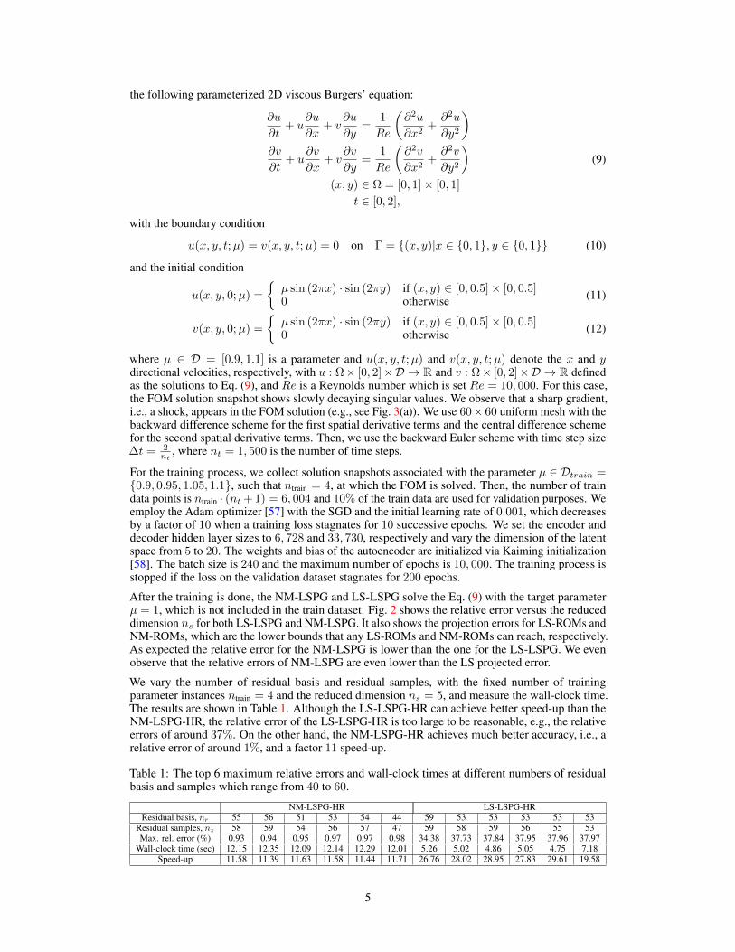
After the training is done, the NM-LSPG and LS-LSPG solve the Eq. (9) with the target parameterµ = 1, which is not included in the train dataset. Fig. 2 shows the relative error versus the reduceddimension ns for both LS-LSPG and NM-LSPG. It also shows the projection errors for LS-ROMs andNM-ROMs, which are the lower bounds that any LS-ROMs and NM-ROMs can reach, respectively.As expected the relative error for the NM-LSPG is lower than the one for the LS-LSPG. We evenobserve that the relative errors of NM-LSPG are even lower than the LS projected error.

We vary the number of residual basis and residual samples, with the fixed number of trainingparameter instances ntrain = 4 and the reduced dimension ns = 5, and measure the wall-clock time.The results are shown in Table 1. Although the LS-LSPG-HR can achieve better speed-up than theNM-LSPG-HR, the relative error of the LS-LSPG-HR is too large to be reasonable, e.g., the relativeerrors of around 37%. On the other hand, the NM-LSPG-HR achieves much better accuracy, i.e., arelative error of around 1%, and a factor 11 speed-up.

Table 1: The top 6 maximum relative errors and wall-clock times at different numbers of residualbasis and samples which range from 40 to 60.

NM-LSPG-HR LS-LSPG-HRResidual basis, nr 55 56 51 53 54 44 59 53 53 53 53 53

Residual samples, nz 58 59 54 56 57 47 59 58 59 56 55 53Max. rel. error (%) 0.93 0.94 0.95 0.97 0.97 0.98 34.38 37.73 37.84 37.95 37.96 37.97

Wall-clock time (sec) 12.15 12.35 12.09 12.14 12.29 12.01 5.26 5.02 4.86 5.05 4.75 7.18Speed-up 11.58 11.39 11.63 11.58 11.44 11.71 26.76 28.02 28.95 27.83 29.61 19.58

5

5 10 15 2010

-3

10-2

10-1

100

(a) Relative errors vs reduced dimensions

0.9 1 1.10

0.05

0.1

0.15

(b) Relative errors vs µ

Figure 2: The comparison of the NM-LSPG-HR and NM-LSPG on the maximum relative errors. Amaximum relative error that is 1 means the ROM failed to solve the problem.

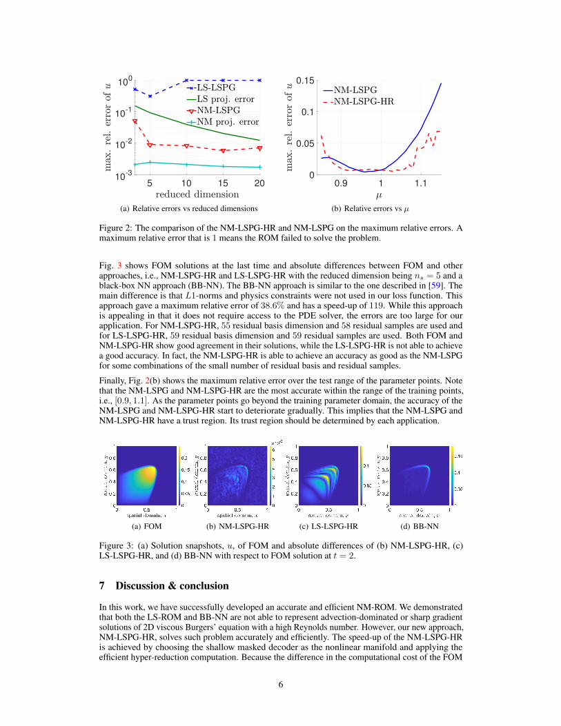
Fig. 3 shows FOM solutions at the last time and absolute differences between FOM and otherapproaches, i.e., NM-LSPG-HR and LS-LSPG-HR with the reduced dimension being ns = 5 and ablack-box NN approach (BB-NN). The BB-NN approach is similar to the one described in [59]. Themain difference is that L1-norms and physics constraints were not used in our loss function. Thisapproach gave a maximum relative error of 38.6% and has a speed-up of 119. While this approachis appealing in that it does not require access to the PDE solver, the errors are too large for ourapplication. For NM-LSPG-HR, 55 residual basis dimension and 58 residual samples are used andfor LS-LSPG-HR, 59 residual basis dimension and 59 residual samples are used. Both FOM andNM-LSPG-HR show good agreement in their solutions, while the LS-LSPG-HR is not able to achievea good accuracy. In fact, the NM-LSPG-HR is able to achieve an accuracy as good as the NM-LSPGfor some combinations of the small number of residual basis and residual samples.

Finally, Fig. 2(b) shows the maximum relative error over the test range of the parameter points. Notethat the NM-LSPG and NM-LSPG-HR are the most accurate within the range of the training points,i.e., [0.9, 1.1]. As the parameter points go beyond the training parameter domain, the accuracy of theNM-LSPG and NM-LSPG-HR start to deteriorate gradually. This implies that the NM-LSPG andNM-LSPG-HR have a trust region. Its trust region should be determined by each application.

(a) FOM (b) NM-LSPG-HR (c) LS-LSPG-HR (d) BB-NN

Figure 3: (a) Solution snapshots, u, of FOM and absolute differences of (b) NM-LSPG-HR, (c)LS-LSPG-HR, and (d) BB-NN with respect to FOM solution at t = 2.

7 Discussion & conclusion

In this work, we have successfully developed an accurate and efficient NM-ROM. We demonstratedthat both the LS-ROM and BB-NN are not able to represent advection-dominated or sharp gradientsolutions of 2D viscous Burgers’ equation with a high Reynolds number. However, our new approach,NM-LSPG-HR, solves such problem accurately and efficiently. The speed-up of the NM-LSPG-HRis achieved by choosing the shallow masked decoder as the nonlinear manifold and applying theefficient hyper-reduction computation. Because the difference in the computational cost of the FOM

6

and NM-LSPG-HR increases as a function of the number of mesh points, we expect more speed-upas the number of mesh points becomes larger.

Compared with the deep neural networks for computer vision and natural language processingapplications, our neural networks are shallow with a small number of parameters. However, thesenetworks were able to capture the variation in our 2D Burgers’ simulations. A main future workfor transferring this work to more complex simulations, will be to find the right balance between ashallow network that is large enough to capture the data variance and yet small enough to run fasterthan the FOM. Another future work will be to find an efficient way of determining the proper size ofthe residual basis and the number of sample points a priori. To find the optimal size of residual basisand the number of sample points for hyper-reduced ROMs, we relied on test results. This issue is notjust for NM-LSPG-HR, but also for LS-LSPG-HR.

Broader Impact

The broader impact of this work will be to accelerate physics simulations to improve design optimiza-tion and control problems, which require thousands of simulation runs to learn an optimal designor viable control strategy. While this is not computationally feasible with high-fidelity FOMs, thedevelopment of the NM-ROMs is an important step in this direction.

Acknowledgments and Disclosure of Funding

This work was performed at Lawrence Livermore National Laboratory and was supported by theLDRD program (project 20-FS-007). Youngkyu was also supported for this work through generousfunding from DTRA. Lawrence Livermore National Laboratory is operated by Lawrence LivermoreNational Security, LLC, for the U.S. Department of Energy, National Nuclear Security Administrationunder Contract DE-AC52-07NA27344 and LLNL-CONF-815209. We declare that there were noconflicting interests of any type during the production of this research.

References[1] Peter Benner, Serkan Gugercin, and Karen Willcox. A survey of projection-based model

reduction methods for parametric dynamical systems. SIAM review, 57(4):483–531, 2015.

[2] Mohamadreza Ghasemi and Eduardo Gildin. Localized model reduction in porous media flow.IFAC-PapersOnLine, 48(6):242–247, 2015.

[3] Rui Jiang and Louis J Durlofsky. Implementation and detailed assessment of a gnat reduced-order model for subsurface flow simulation. Journal of Computational Physics, 379:192–213,2019.

[4] Yanfang Yang, Mohammadreza Ghasemi, Eduardo Gildin, Yalchin Efendiev, Victor Calo,et al. Fast multiscale reservoir simulations with pod-deim model reduction. SPE Journal,21(06):2–141, 2016.

[5] Huanhuan Yang and Alessandro Veneziani. Efficient estimation of cardiac conductivities viapod-deim model order reduction. Applied Numerical Mathematics, 115:180–199, 2017.

[6] Pengfei Zhao, Cai Liu, and Xuan Feng. Pod-deim based model order reduction for the sphericalshallow water equations with turkel-zwas finite difference discretization. Journal of AppliedMathematics, 2014, 2014.

[7] R Stefanescu and Ionel Michael Navon. Pod/deim nonlinear model order reduction of an adiimplicit shallow water equations model. Journal of Computational Physics, 237:95–114, 2013.

[8] M Mordhorst, Timm Strecker, D Wirtz, Thomas Heidlauf, and Oliver Röhrle. Pod-deimreduction of computational emg models. Journal of Computational Science, 19:86–96, 2017.

[9] Gabriel Dimitriu, Ionel M Navon, and Razvan Stefanescu. Application of pod-deim approachfor dimension reduction of a diffusive predator-prey system with allee effect. In Internationalconference on large-scale scientific computing, pages 373–381. Springer, 2013.

7

[10] Harbir Antil, Matthias Heinkenschloss, Ronald HW Hoppe, Christopher Linsenmann, andAchim Wixforth. Reduced order modeling based shape optimization of surface acoustic wavedriven microfluidic biochips. Mathematics and Computers in Simulation, 82(10):1986–2003,2012.

[11] David Amsallem, Matthew Zahr, Youngsoo Choi, and Charbel Farhat. Design optimization usinghyper-reduced-order models. Structural and Multidisciplinary Optimization, 51(4):919–940,2015.

[12] Youngsoo Choi, Gabriele Boncoraglio, Spenser Anderson, David Amsallem, and CharbelFarhat. Gradient-based constrained optimization using a database of linear reduced-ordermodels. Journal of Computational Physics, page 109787, 2020.

[13] Youngsoo Choi, Geoffrey Oxberry, Daniel White, and Trenton Kirchdoerfer. Acceleratingdesign optimization using reduced order models. arXiv preprint arXiv:1909.11320, 2019.

[14] Hongfei Fu, Hong Wang, and Zhu Wang. Pod/deim reduced-order modeling of time-fractionalpartial differential equations with applications in parameter identification. Journal of ScientificComputing, 74(1):220–243, 2018.

[15] Rémi Abgrall, David Amsallem, and Roxana Crisovan. Robust model reduction by l1-normminimization and approximation via dictionaries: application to nonlinear hyperbolic problems.Advanced Modeling and Simulation in Engineering Sciences, 3(1):1–16, 2016.

[16] Julius Reiss, Philipp Schulze, Jörn Sesterhenn, and Volker Mehrmann. The shifted properorthogonal decomposition: A mode decomposition for multiple transport phenomena. SIAMJournal on Scientific Computing, 40(3):A1322–A1344, 2018.

[17] Kevin Carlberg, Charbel Farhat, Julien Cortial, and David Amsallem. The gnat method fornonlinear model reduction: effective implementation and application to computational fluiddynamics and turbulent flows. Journal of Computational Physics, 242:623–647, 2013.

[18] Kevin Carlberg, Youngsoo Choi, and Syuzanna Sargsyan. Conservative model reduction forfinite-volume models. Journal of Computational Physics, 371:280–314, 2018.

[19] Youngsoo Choi, Deshawn Coombs, and Robert Anderson. Sns: a solution-based nonlinearsubspace method for time-dependent model order reduction. SIAM Journal on ScientificComputing, 42(2):A1116–A1146, 2020.

[20] Dunhui Xiao, Fangxin Fang, Andrew G Buchan, Christopher C Pain, Ionel Michael Navon,Juan Du, and G Hu. Non-linear model reduction for the navier–stokes equations using residualdeim method. Journal of Computational Physics, 263:1–18, 2014.

[21] PG Constantine and G Iaccarino. Reduced order models for parameterized hyperbolic con-servations laws with shock reconstruction. Center for Turbulence Research Annual Brief,2012.

[22] Youngsoo Choi, Peter Brown, Bill Arrighi, Robert Anderson, and Kevin Huynh. Space–timereduced order model for large-scale linear dynamical systems with application to boltzmanntransport problems. Journal of Computational Physics, P109845, 2020.

[23] Youngsoo Choi and Kevin Carlberg. Space–time least-squares petrov–galerkin projection fornonlinear model reduction. SIAM Journal on Scientific Computing, 41(1):A26–A58, 2019.

[24] Tommaso Taddei and Lei Zhang. Space-time registration-based model reduction of parameter-ized one-dimensional hyperbolic pdes. arXiv preprint arXiv:2004.06693, 2020.

[25] Kevin Carlberg. Adaptive h-refinement for reduced-order models. International Journal forNumerical Methods in Engineering, 102(5):1192–1210, 2015.

[26] Donsub Rim, Scott Moe, and Randall J LeVeque. Transport reversal for model reduction ofhyperbolic partial differential equations. SIAM/ASA Journal on Uncertainty Quantification,6(1):118–150, 2018.

8

[27] Eric J Parish and Kevin T Carlberg. Windowed least-squares model reduction for dynamicalsystems. arXiv preprint arXiv:1910.11388, 2019.

[28] Benjamin Peherstorfer. Model reduction for transport-dominated problems via online adaptivebases and adaptive sampling. arXiv preprint arXiv:1812.02094, 2018.

[29] G Welper. Transformed snapshot interpolation with high resolution transforms. SIAM Journalon Scientific Computing, 42(4):A2037–A2061, 2020.

[30] Isaac E Lagaris, Aristidis Likas, and Dimitrios I Fotiadis. Artificial neural networks for solvingordinary and partial differential equations. IEEE transactions on neural networks, 9(5):987–1000, 1998.

[31] MWMG Dissanayake and N Phan-Thien. Neural-network-based approximations for solvingpartial differential equations. communications in Numerical Methods in Engineering, 10(3):195–201, 1994.

[32] B Ph van Milligen, V Tribaldos, and JA Jiménez. Neural network differential equation andplasma equilibrium solver. Physical review letters, 75(20):3594, 1995.

[33] Andrew J Meade Jr and Alvaro A Fernandez. The numerical solution of linear ordinarydifferential equations by feedforward neural networks. Mathematical and Computer Modelling,19(12):1–25, 1994.

[34] Maziar Raissi, Paris Perdikaris, and George E Karniadakis. Physics-informed neural networks:A deep learning framework for solving forward and inverse problems involving nonlinear partialdifferential equations. Journal of Computational Physics, 378:686–707, 2019.

[35] Ricky TQ Chen, Yulia Rubanova, Jesse Bettencourt, and David K Duvenaud. Neural ordinarydifferential equations. In Advances in neural information processing systems, pages 6571–6583,2018.

[36] Yuehaw Khoo, Jianfeng Lu, and Lexing Ying. Solving parametric pde problems with artificialneural networks. arXiv preprint arXiv:1707.03351, 2017.

[37] Zichao Long, Yiping Lu, Xianzhong Ma, and Bin Dong. Pde-net: Learning pdes from data. InInternational Conference on Machine Learning, pages 3208–3216, 2018.

[38] Christian Beck, E Weinan, and Arnulf Jentzen. Machine learning approximation algorithmsfor high-dimensional fully nonlinear partial differential equations and second-order backwardstochastic differential equations. Journal of Nonlinear Science, 29(4):1563–1619, 2019.

[39] Yinhao Zhu, Nicholas Zabaras, Phaedon-Stelios Koutsourelakis, and Paris Perdikaris. Physics-constrained deep learning for high-dimensional surrogate modeling and uncertainty quantifica-tion without labeled data. Journal of Computational Physics, 394:56–81, 2019.

[40] Jens Berg and Kaj Nyström. A unified deep artificial neural network approach to partialdifferential equations in complex geometries. Neurocomputing, 317:28–41, 2018.

[41] Justin Sirignano and Konstantinos Spiliopoulos. Dgm: A deep learning algorithm for solvingpartial differential equations. Journal of computational physics, 375:1339–1364, 2018.

[42] Jiequn Han, Arnulf Jentzen, and E Weinan. Solving high-dimensional partial differentialequations using deep learning. Proceedings of the National Academy of Sciences, 115(34):8505–8510, 2018.

[43] Lu Lu, Pengzhan Jin, and George Em Karniadakis. Deeponet: Learning nonlinear operators foridentifying differential equations based on the universal approximation theorem of operators.arXiv preprint arXiv:1910.03193, 2019.

[44] Lu Lu, Xuhui Meng, Zhiping Mao, and George E Karniadakis. Deepxde: A deep learninglibrary for solving differential equations. arXiv preprint arXiv:1907.04502, 2019.

[45] Guofei Pang, Lu Lu, and George Em Karniadakis. fpinns: Fractional physics-informed neuralnetworks. SIAM Journal on Scientific Computing, 41(4):A2603–A2626, 2019.

9

[46] Dongkun Zhang, Lu Lu, Ling Guo, and George Em Karniadakis. Quantifying total uncertainty inphysics-informed neural networks for solving forward and inverse stochastic problems. Journalof Computational Physics, 397:108850, 2019.

[47] E Weinan and Bing Yu. The deep ritz method: a deep learning-based numerical algorithm forsolving variational problems. Communications in Mathematics and Statistics, 6(1):1–12, 2018.

[48] Juncai He, Lin Li, Jinchao Xu, and Chunyue Zheng. Relu deep neural networks and linear finiteelements. arXiv preprint arXiv:1807.03973, 2018.

[49] Kookjin Lee and Kevin T Carlberg. Model reduction of dynamical systems on nonlinear mani-folds using deep convolutional autoencoders. Journal of Computational Physics, 404:108973,2020.

[50] Kookjin Lee and Kevin Carlberg. Deep conservation: A latent dynamics model for exactsatisfaction of physical conservation laws. arXiv preprint arXiv:1909.09754, 2019.

[51] Mark A Kramer. Nonlinear principal component analysis using autoassociative neural networks.AIChE journal, 37(2):233–243, 1991.

[52] Saifon Chaturantabut and Danny C Sorensen. Nonlinear model reduction via discrete empiricalinterpolation. SIAM Journal on Scientific Computing, 32(5):2737–2764, 2010.

[53] Zlatko Drmac and Serkan Gugercin. A new selection operator for the discrete empiricalinterpolation method—improved a priori error bound and extensions. SIAM Journal on ScientificComputing, 38(2):A631–A648, 2016.

[54] Zlatko Drmac and Arvind Krishna Saibaba. The discrete empirical interpolation method:Canonical structure and formulation in weighted inner product spaces. SIAM Journal on MatrixAnalysis and Applications, 39(3):1152–1180, 2018.

[55] Richard Everson and Lawrence Sirovich. Karhunen–loeve procedure for gappy data. JOSA A,12(8):1657–1664, 1995.

[56] Kevin Carlberg, Charbel Bou-Mosleh, and Charbel Farhat. Efficient non-linear model reduc-tion via a least-squares petrov–galerkin projection and compressive tensor approximations.International Journal for Numerical Methods in Engineering, 86(2):155–181, 2011.

[57] Diederik P. Kingma and Jimmy Ba. Adam: A method for stochastic optimization, 2014.

[58] Kaiming He, Xiangyu Zhang, Shaoqing Ren, and Jian Sun. Delving deep into rectifiers:Surpassing human-level performance on imagenet classification. In Proceedings of the IEEEinternational conference on computer vision, pages 1026–1034, 2015.

[59] Byungsoo Kim, Vinicius C. Azevedo, Nils Thuerey, Theodore Kim, Markus H. Gross, andBarbara Solenthaler. Deep fluids: A generative network for parameterized fluid simulations.CoRR, abs/1806.02071, 2018.

10