Efficient exploration of the lensed CMB likelihood.

Julien Carron

Acknow. Antony Lewis, Julien Peloton

Chania 26 May 2016

CMB Lensing :

• 2 arcmin deflection of CMB photons on their path from last scattering surface to us by the large scale structure.

• Valuable cosmological signal in itself, that also correlates to other large scale structure tracers.

• Very linear (z ~ 2), no intrinsic alignments, no photo-z’s to obtain…

• The lensing potential is traditionally reconstructed via estimators quadratic in the CMB maps (Okamoto & Hu 2003)

CMB lensing has just started with Planck. But can we do even better ?

Reconstruction noise on Fourier modes of the displacement.

Motivations :

Why bother ? The quadratic estimator works, is fast, and do promise great science.

1. For experiments with B-mode sensitivity below 5 muK arcmin, we know the quadratic estimator may be grossly suboptimal. (Should be possible to solve for B = 0)

Motivations :

The quadratic estimator works, is fast, and promises great science. Why bother ?

1. For experiments with B-mode sensitivity below 5 muK arcmin, we know the quadratic estimator may be grossly suboptimal. (Becomes possible to solve for B = 0)

2. Lensing power spectra such as produced by Planck are cleaned (or can tentatively be cleaned) from several biases, N0, N1, (N 3/2 … ), point sources, etc. Not so for the potential map.

3. If the use of the full likelihood is possible, it also opens the door to new / (better ?) inference approaches. (such as joint temperature / lensing reconstruction, or B-mode delensing e.g.)

Model for the data

• Data vector easily has a million entry or more.

• We want to reconstruct the entire displacement field.

(B beam, D deflection, n noise)

and / or Pol.Gaussian

Likelihood Prior

• Dream : direct sampling (Anderes & al 2015)

• Iterative estimate (approx. posterior) (Hirata & Seljak 2003)

This talk :

• Exact maximum a posteriori (MAP) solver

• Preliminary results on B-mode delensing

Beyond the quadratic estimator :

Evaluation of the likelihood is no piece of cake.

• Big C-inverse. Data vector can have a million or more entries. —> but can be made to work

• Impossible determinant evaluation. —> but we only need the derivatives to find the maximum a posteriori point. The derivatives can be evaluated with MCs.

• It is possible to apply the anisotropic CMB covariance to a data vector in linear time.—> conjugate gradient descent to solve for the inverse covariance.

Steps :1. Beam convolution 2. Apply backward displacement (delensing) 3. Divide by magnification matrix 4. Apply isotropic CMB Cl’s in harmonic space 5. Apply forward displacement 6. Beam convolution 7. Add noise

Quadratic Piece

• Numerical cost : - Inversion of the displacement field (easy for LCDM, NR implementation) + 2 lensing operations x # c.g. iterations x (1,2,3) for T, Pol. ,T+Pol. +4 harmonic transforms x # c.g. iterations x (1,2,3) for T, Pol. ,T+Pol.

• Turns out the # of c.g. iterations does not depend on fsky. —> Costly, but still linear complexity.

Quadratic Piece

Mean field

—> In principle, just repeat the previous step as much as necessary.

But : MC noise (~ N0 lensing bias) is much larger than the mean field itself. To be precise, one needs a lot of simulations.

Mean field

—> In principle, just repeat the previous step as much as necessary.

But : MC noise (~ N0 lensing bias) is much larger than the mean field itself. To be precise, one needs a lot of simulations.

The MC noise can be decreased by an order of magnitude of more using two tricks :

1. Changes in weights A, B leaving the diagonal of the RHS invariant. 2. Subtract the same estimate in the absence of displacement.

Mean field

T.

Pol.

Trick 1 Trick 2

2 layers of iterations

• Outer layer : search for the MAP point using gradient information. Starting point the quadratic estimate. Use L-BFGS quasi-Newton scheme, inverse covariance matrix comes for free.

• Inner layer : calculation of the gradient. (Conjugate gradient) Dominates the numerical cost.

Quadratic estimator

MAP point

Numerical Cost

With most naive preconditioner (isotropic covariance) :

Beam ~ few arcmin. Deflection coherent over ~ degree.—> Pick a preconditioner for which beam and deflection commute.

Beam ~ few arcmin. Deflection coherent over ~ degree.—> Pick a preconditioner for which beam and deflection commute.

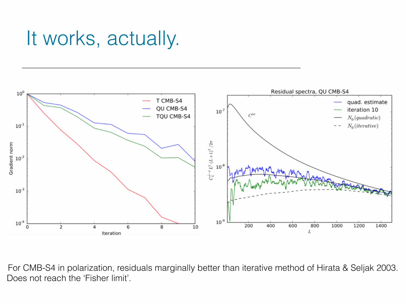
It works, actually.

For CMB-S4 in polarization, residuals marginally better than iterative method of Hirata & Seljak 2003. Does not reach the ‘Fisher limit’.

B-mode delensing

Standard method : Use displacement inferred on small scales to delens the large scale B-mode map.

Very much inline with current improvement forecasts for CMB-S4

Delensing : using BB in likelihood.

Discarding ell > 200, standard reconstruction Keeping full range, including BB in likelihoodPrelim

inary

r = 0.01, fsky = 0.015

Conclusions

• Flexible, easy to use, parallel python code solving for the MAP lensing potential map, in the flat sky approximation. Tested up to CMB-S4 configurations. Contains thoroughly tested standard minimal variance quadratic estimators libraries and lensed CMBs simulations libraries.

• Residuals decreased by a factor of 2 for CMB-S4. Promising preliminary results for B-mode delensing.

Thank you !

Thank you !