Eemd Examples
20
Improving the Performance of the HHT using Ensemble Empirical Mode Decomposition Daniel Bowman January 10, 2014 Contents 1 Introduction 1 2 Eliminating Spline Fitting Problems 2 2.1 Code ................................ 3 2.2 Figures ............................... 4 3 Reducing Mode Mixing 8 3.1 Code ................................ 8 3.2 Figures ............................... 10 4 Transient Seismic Event Analyzed with EEMD 15 4.1 Code ................................ 16 4.2 Figures ............................... 17 1 Introduction This vignette shows how the ensemble empirical mode decomposition method (EEMD) can improve the empirical mode decomposition (EMD) method and the resulting Hilbert spectrogram. The EEMD is a noise assisted version of the EMD method. It was developed to reduce aliasing and mode mixing that can occur during EMD. For more information, see Wu and Huang (2009) “Ensemble Empirical Mode Decomposition: A Noise Assisted Data Analysis Method.” 1
-
Upload
humbang-purba -
Category
Documents
-
view
228 -
download
10
description
signal processing
Transcript of Eemd Examples

Improving the Performance of the HHT usingEnsemble Empirical Mode Decomposition
Daniel Bowman
January 10, 2014
Contents
1 Introduction 1
2 Eliminating Spline Fitting Problems 22.1 Code . . . . . . . . . . . . . . . . . . . . . . . . . . . . . . . . 32.2 Figures . . . . . . . . . . . . . . . . . . . . . . . . . . . . . . . 4
3 Reducing Mode Mixing 83.1 Code . . . . . . . . . . . . . . . . . . . . . . . . . . . . . . . . 83.2 Figures . . . . . . . . . . . . . . . . . . . . . . . . . . . . . . . 10
4 Transient Seismic Event Analyzed with EEMD 154.1 Code . . . . . . . . . . . . . . . . . . . . . . . . . . . . . . . . 164.2 Figures . . . . . . . . . . . . . . . . . . . . . . . . . . . . . . . 17
1 Introduction
This vignette shows how the ensemble empirical mode decomposition method(EEMD) can improve the empirical mode decomposition (EMD) method andthe resulting Hilbert spectrogram. The EEMD is a noise assisted version ofthe EMD method. It was developed to reduce aliasing and mode mixing thatcan occur during EMD. For more information, see Wu and Huang (2009)“Ensemble Empirical Mode Decomposition: A Noise Assisted Data AnalysisMethod.”
1

This vignette examines three signals. The first signal demonstrates howthe EEMD can improve the quality of intrinsic mode functions (IMFs), par-ticularly at the beginning and end of the signal.
The second signal has two sinusoids with Gaussian white noise added.This example shows how the EEMD method can improve the IMF set andthe resulting Hilbert spectrogram.
The third signal is a transient event recorded at Deception Island vol-cano, Antarctica. I show how the EEMD can extract meaningful informationfrom a signal previously thought to be too short for spectral analysis. I alsodemonstrate the higher time frequency resolution of the Hilbert spectrogramas opposed to the Fourier spectrogram.
WARNING: The EEMD code in this vignette takes severalhours to run.
2 Eliminating Spline Fitting Problems
Consider the following signal:
x(t) = sin(2πt+ 0.5 sin(πt))e−(t−50)2)
200 + sin(π
10t) (1)
While the EMD successfully removes the nonlinear signal from the lowerfrequency sinusoid, the first and second IMF contain unusual oscillations inthe first 20 and last 20 seconds of the signal (Fig. 1). These oscillationsare not implied in the signal equation and likely represent problems with thespline fitting method in the EMD.
If low amplitude Gaussian white noise is added to the signal, the splinefitting issue is solved (Fig. 2). However, this creates a lot more IMFs, and thetransient nonlinear signal is now distributed across multiple IMFs rather thanresiding on a single IMF. This problem is called mode mixing and reflects thefact that random noise populates all time scales equally. Mode mixing cancause aliasing in the Hilbert transform because it disturbs local symmetry inthe affected IMFs.
Each trial of the EEMD method adds a different white noise set to thesignal and performs EMD. If this is done enough times, the averaged IMFset from all the trials approaches the “true” signal . After EEMD, the splinefitting has been improved. Although the higher frequency signal remains on
2

two IMFs (Fig. 3), the two averaged modes are smoother compared to thesignal with only one EMD run (Fig. 2).
2.1 Code
EMD with no added noise
> library(hht)
> dt=0.01
> tt=seq_len(10000)*dt
> sig=sin(2*pi*tt+0.5*sin(pi*tt))*exp(-(tt-50)^2/100)+sin(pi*tt/10)
> emd.result=Sig2IMF(sig, tt)
> PlotIMFs(emd.result)
EMD with added noise
> set.seed(628)
> sig2=sin(2*pi*tt+0.5*sin(pi*tt))*exp(-(tt-50)^2/100)+
+ sin(pi*tt/10)+rnorm(length(sig), 0, 0.01)
> emd.result=Sig2IMF(sig2, tt)
> PlotIMFs(emd.result)
Perform EEMD
> trials=100
> nimf=11
> noise.amp=0.01
> trials.dir="example_1"
> EEMD(sig2, tt, noise.amp, trials, nimf,
+ trials.dir = trials.dir, verbose = FALSE)
[1] "Created trial directory: example_1"
> EEMD.result=EEMDCompile(trials.dir, trials, nimf)
Calculate and Plot Averaged IMFs
> resift.rule="max.var"
> resift.result=EEMDResift(EEMD.result,
+ resift.rule = resift.rule)
3

> time.span=c(0, 100)
> imf.list=c(3:7)
> os=TRUE
> res=FALSE
> PlotIMFs(resift.result)
2.2 Figures
4

Time (s)
0 20 40 60 80 100
Res
idue
IMF
2IM
F 1
Sig
nal
Figure 1: EMD of signal in Equation 1. A total of 2 IMFs were returned.
5

Time (s)
0 20 40 60 80 100
Res
idue
IMF
7IM
F 5
IMF
3IM
F 1
Figure 2: EMD of signal in Equation 1 with random Gaussian noise added.
6

Time (s)
0 20 40 60 80 100
Res
idue
IMF
8IM
F 6
IMF
4IM
F 2
Sig
nal
Figure 3: Major IMFs from EEMD of signal in Equation 1.
7

3 Reducing Mode Mixing
Even a well behaved stationary time series will have problems if there israndom noise in addition to the signal. Fortunately, the EEMD is able tocounteract the effect of a noisy signal by averaging a large number of trialstogether. As the number of trials grows, the signal tends to emerge from theaveraged IMF set.
This example’s time series has the form
x(t) = 2 sin(2πt) + 0.5 sin(12πt) + N (0, 0.4) (2)
whereN (0, 0.4)
produces random Gaussian noise with a mean of 0 and a standard deviationof 0.4. In theory, the EMD should produce one IMF showing the 2 sin(2πt)component and one IMF showing the 0.5 sin(12πt) component. However,the presence of noise creates many more IMFs and also causes severe modemixing. The most obvious mode mixing occurs where portions of the highfrequency sinusoid switch back and forth between IMF 2 and IMF 3. IMF4 and IMF 5 both contain portions of the lower frequency, creating severedistortion in that signal band as well (Fig. 4).
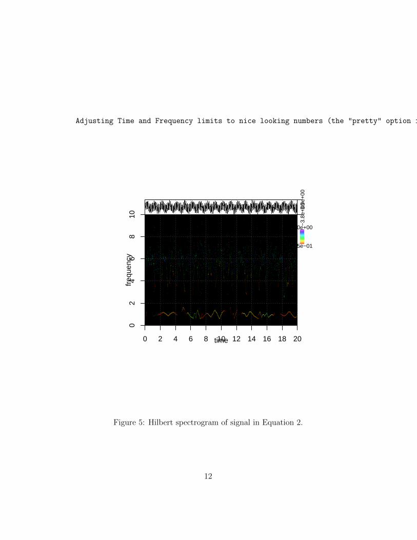
The Hilbert spectrogram of this time series should show strong continuousfrequency bands at 1 Hz and 6 Hz. However, the mode mixing produces achaotic spectrogram with an intermittent low frequency signal around 0.5 Hzand a scattered high frequency signal between 4 and 8 Hz (Fig. 5). Aftera 100 trial EEMD run, the averaged IMF set looks better than the originalEMD (Fig. 6).
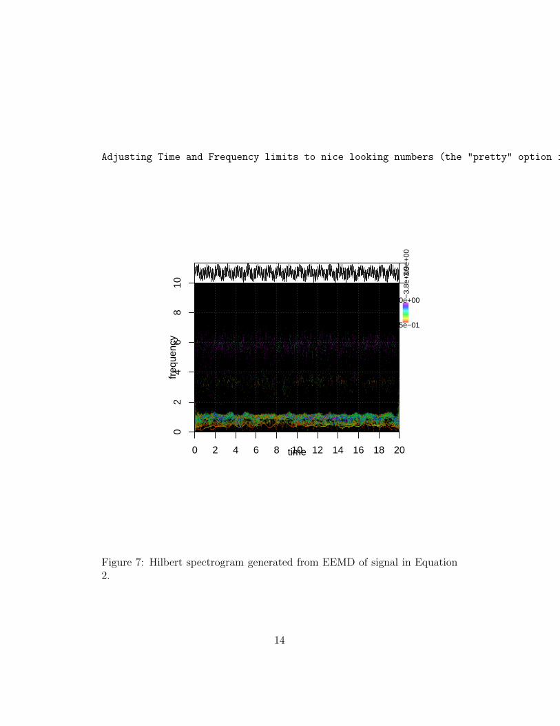
The EEMD Hilbert spectrogram is a marked improvement over the orig-inal Hilbert spectrogram (Fig. 7). There are two continuous bands of energythat correspond with the sinusoids in Equation 2. While the 6 Hz band isstill noisy, it is less scattered than in the original spectrogram in Figure 5.
3.1 Code
EMD of noisy signal
> library(hht)
> set.seed(628)
8

> dt=0.01
> tt=seq_len(2000)*dt
> sig=sin(2*pi*tt) + 2*sin(12*pi*tt)+rnorm(length(tt), 0, 0.4)
> emd.result=Sig2IMF(sig, tt)
> PlotIMFs(emd.result)
Hilbert spectrogram of noisy signal
> dfreq = 0.05
> freq.span = c(0, 10)
> hgram=HHRender(emd.result, dt, dfreq, freq.span = freq.span,
+ verbose = FALSE)
> time.span=c(0, 20)
> freq.span=c(0, 10)
> amp.span=c(0.75, 3)
> HHGramImage(hgram, time.span = time.span, freq.span = freq.span,
+ amp.span = amp.span, pretty = TRUE,
+ img.y.format = "%.0f", img.x.format = "%.0f")
Adjusting Time and Frequency limits to nice looking numbers (the "pretty" option is currently set to TRUE)
Run EEMD
> trials=100
> nimf=9
> noise.amp=0.4
> trials.dir="example_2"
> EEMD(sig, tt, noise.amp, trials, nimf,
+ trials.dir = trials.dir, verbose = FALSE)
[1] "Created trial directory: example_2"
> EEMD.result=EEMDCompile(trials.dir, trials, nimf)
Generate averaged IMF set
> PlotIMFs(EEMD.result, imf.list = c(2, 3, 5),
+ res = FALSE, fit.line = TRUE)
Render and plot EEMD Hilbert spectrogram
9

> freq.span=c(0, 10)
> dfreq=0.05
> hgram=HHRender(EEMD.result, dt, dfreq,
+ freq.span = freq.span, verbose = FALSE)
> time.span=c(0, 20)
> freq.span=c(0, 10)
> amp.span=c(0.75, 3)
> cluster.span=c(5, 100)
> HHGramImage(hgram, time.span = time.span, freq.span = freq.span,
+ amp.span = amp.span, cluster.span = cluster.span, pretty = TRUE,
+ img.y.format = "%.0f", img.x.format = "%.0f")
Adjusting Time and Frequency limits to nice looking numbers (the "pretty" option is currently set to TRUE)
3.2 Figures
10

Time (s)
0 5 10 15 20
Res
idue
IMF
6IM
F 4
IMF
2S
igna
l
Figure 4: EMD of signal in Equation 2.
11
Adjusting Time and Frequency limits to nice looking numbers (the "pretty" option is currently set to TRUE)
02
46
810
0 2 4 6 8 10 12 14 16 18 20
−3.
8e+
003.9e
+00
freq
uenc
y
time
7.5e−01
3.0e+00
Figure 5: Hilbert spectrogram of signal in Equation 2.
12

Time (s)
0 5 10 15 20
IMF
5IM
F 3
IMF
2S
igna
l
Figure 6: Averaged IMF set generated from EEMD of signal in Equation 2.Note that the three IMFs shown match the signal content quite well (the redline shows the sum of the IMFs, the black line is the original signal).
13
Adjusting Time and Frequency limits to nice looking numbers (the "pretty" option is currently set to TRUE)
02
46
810
0 2 4 6 8 10 12 14 16 18 20
−3.
8e+
003.9e
+00
freq
uenc
y
time
7.5e−01
3.0e+00
Figure 7: Hilbert spectrogram generated from EEMD of signal in Equation2.
14

4 Transient Seismic Event Analyzed with EEMD
A network of ocean bottom seismometers was deployed in Port Foster (theflooded caldera of Deception Island volcano) in 2005. These instrumentsrecorded numerous transient seismic events. One of these events has beenincluded as an example data set in this R package. The following exampledemonstrates how detailed spectral information can be extracted from thissignal using the EEMD method.
The EEMD method recovers three main IMFs: a high amplitude, highfrequency component, a high amplitude, low frequency component and a lowfrequency, low amplitude component (Fig. 8). While the presence of a highfrequency component is clear from the original signal, the spindle shape ofthis component is not obvious until it is decomposed into an IMF. Althoughthis could have been discovered by using a bandpass filter, the signal couldhave been distorted because of the transient nature of the waveform and thefact that this component has frequency modulation. Therefore, the EEMDhas already recovered potentially valuable information on the different com-ponents of this signal.
The EEMD Hilbert spectrogram shows that each of the three componentsvaries in frequency throughout the signal (Fig. 9). The high frequencycomponent has energy between 15 and 20 Hz, dropping to around 13 Hz inabout a quarter of a second. The low frequency, high amplitude componentstarts at around 6 Hz, glides to below 5 Hz over a half second, then risesin frequency again for another second or so before tapering off. The lowfrequency, low amplitude component decreases from around 5 Hz to around2 Hz over less than a second.
The Fourier spectrogram cannot resolve such fine details in this signal(Fig. 10). It is difficult to determine if there is frequency gliding in the Fourierspectrogram due to the coarseness of the frequency resolution. This problemcould be alleviated by shortening the time window, but that would maskthe contribution of lower frequency elements of the signal. Also, the Fourierspectrogram shows energy arriving slightly before 6.5 seconds, whereas theseismogram shows the main signal starting just after 6.5 seconds. However,the Hilbert spectrogram shows spectral energy arriving just after 6.5 seconds,thus providing better agreement with the seismogram.
15

4.1 Code
Run EEMD
> library(hht)
> data(PortFosterEvent)
> set.seed(628)
> trials=100
> nimf=8
> noise.amp=6.4e-07
> trials.dir="example_3"
> EEMD(sig, tt, noise.amp, trials, nimf,
+ trials.dir = trials.dir, verbose = FALSE)
[1] "Created trial directory: example_3"
> EEMD.result=EEMDCompile(trials.dir, trials, nimf)
Create averaged IMF set
> resift.rule="max.var"
> resift.result=EEMDResift(EEMD.result, resift.rule = resift.rule)
> time.span=c(5, 10)
> imf.list=1:3
> os=TRUE
> res=FALSE
> fit.line=TRUE
> PlotIMFs(resift.result, time.span, imf.list, os, res, fit.line)
Render and display Hilbert spectrogram
> freq.span=c(0, 30)
> dt = 0.01
> dfreq=0.05
> hgram=HHRender(EEMD.result, dt, dfreq,
+ freq.span = freq.span, verbose = FALSE)
> time.span=c(5, 9)
> freq.span=c(0, 25)
> amp.span=c(1e-06, 3e-05)
> cluster.span=c(4, 100)
> HHGramImage(hgram, time.span = time.span, freq.span = freq.span,
+ amp.span = amp.span, cluster.span = cluster.span)
16
Render and display Fourier spectrogram
> dt=mean(diff(tt))
> ft=list()
> ft$nfft=4096
> ft$ns=30
> ft$nov=29
> time.span=c(5, 10)
> freq.span=c(0, 25)
> amp.span=c(0.00001, 0.001)
> FTGramImage(sig, dt, ft, time.span = time.span,
+ freq.span = freq.span, amp.span = amp.span)
4.2 Figures
17

Time (s)
5 6 7 8 9 10
IMF
3IM
F 2
IMF
1S
igna
l
Figure 8: Averaged IMFs from EEMD of transient seismic signal. The redline shows the sum of displayed IMFs; the black line shows the original signal.
18

0.00
6.25
12.5
018
.75
25.0
0
5.00 5.89 6.78 7.67 8.56
6.6e
−047
.3e−
04
freq
uenc
y
time
1.0e−06
3.0e−05
Figure 9: Hilbert spectrogram of EEMD of transient seismic signal.
19

0.00
6.24
12.4
818
.72
24.9
6
5.13 6.19 7.25 8.31 9.37
6.6e
−047
.3e−
04
freq
uenc
y
time
1.0e−05
1.0e−03
Figure 10: Fourier spectrogram of transient seismic signal.
20