Eelgrass (Zostera marina L. Restoration in Puget … (Zostera marina L.) Restoration in Puget ......

PNNL-23635

Eelgrass (Zostera marina L.) Restoration in Puget Sound: Development and Testing of Tools for Optimizing Site Selection

September 2014

RM Thom J Vavrinec JL Gaeckle L Aston KE Buenau DL Woodruff AB Borde

PNNL-23635

Eelgrass (Zostera marina L.) Restoration in Puget Sound: Development and Testing of Tools for Optimizing Site Selection RM Thom J Vavrinec JL Gaeckle L Aston KE Buenau DL Woodruff AB Borde September 2014 Prepared for the U.S. Department of Energy under Contract DE-AC05-76RL01830 Pacific Northwest National Laboratory Richland, Washington 99352

iii

Abstract

The restoration of eelgrass (Zostera marina L.) as a critical ecosystem component and indicator of environmental health, is a high priority in Washington State’s Puget Sound, where the goal is to increase the current eelgrass coverage by 20 percent (i.e., 4,000 ha) by 2020. In a region as large and complex as Puget Sound, locating areas to restore eelgrass effectively and efficiently is a challenge. We developed a set of tools to identify and test potential restoration sites, as well as to identify stressors affecting eelgrass and other barriers to its recovery. These tools consist of numerical models of hydrodynamics and eelgrass biomass; a spatially explicit habitat suitability model that incorporates information from predictive models as well as current and past eelgrass cover, substrate, and stressors; information elicited from shoreline planners and seagrass experts; test plantings and monitoring of light, temperature, and survival; and maps and recommendations summarizing all of these components to aid in identifying potential restoration sites. Our habitat suitability model identified 3,000 ha of highly suitable potential habitat where eelgrass is not currently present and an additional 4,401 ha of moderately suitable eelgrass habitat. Surveys of stakeholders identified dredging/filling, shoreline development, water quality, and commercial aquaculture as the most significant stressors on eelgrass, and noted that new regulations and improved enforcement of existing regulations would be necessary to ensure continued recovery and protection of eelgrass. Test plantings at several locations in south Puget Sound (i.e., Joemma State Park and Zangle Cove) suggested the possibility of successful restoration. Test plantings at Anderson Island, Liberty Bay, and the head of Westcott Bay were unsuccessful, which suggested that further investment in restoration at those locations would be unadvisable unless stressors were identified and abated. Overall, we found that our approach provides a foundation for identifying and testing potential restoration sites as well as identifying information needs and potential management actions toward reducing stressors and increasing eelgrass cover and health to meet the challenging restoration goal.

vii

Acknowledgments

This project has been funded wholly or in part by the U.S. Environmental Protection Agency (EPA), under assistance agreement PC00J29801 to Washington Department of Fish and Wildlife. The contents of this document do not necessarily reflect the views and policies of the EPA, nor does mention of trade names or commercial products constitute endorsement or recommendation for use.

This manuscript is the culmination of two years of work and several technical reports. We thank Helen Berry and Fred Short from the Washington Department of Natural Resources, and Jim Kaldy from the EPA for guidance, information, and other knowledge about eelgrass in Puget Sound as well as feedback and assistance in this project. We also thank several staff from the Pacific Northwest National Laboratory (PNNL): Shon Zimmerman for providing support on transplanting and mapping efforts, Heida Diefenderfer for assisting with the geospatial report, Lyle Hibler for working on the eelgrass model and the hydrodynamic and water quality model interface, Tarang Khangaonkar and Wen Long for providing the hydrodynamic model output, and Susan Ennor for editing and formatting assistance. Special thanks to Allie Simpson, a PNNL intern, who provided data for eelgrass modeling and field support and to all of the volunteers from the Washington Conservation Corps who helped with bundling eelgrass for transplanting. Finally, we would finally like to thank Greg Williams, Keith Marcoe, Adrian Burd, Keith Merkel, Doug Bulthuis, Jim Brennan, Randy Carman, and Kelly Andrews who provided reviews of the technical reports and Scott Marion and Sandy Wyllie-Echeverria for reviewing this manuscript.

ix

Acronyms and Abbreviations

DNR Washington State Department of Natural Resources

EBM biomass productivity potential

ECI Environmental Condition Index

EPA U.S. Environmental Protection Agency

ERP eelgrass restoration potential

FVCOM Finite Volume Coastal Ocean Model

GIS geographic information system

GPP gross photosynthetic production

MLLW mean lower low water

NAVD88 North American Vertical Datum of 1988

PAR photosynthetically active radiation

PNNL Pacific Northwest National Laboratory

PSNERP Puget Sound Nearshore Ecosystem Restoration Project

PVC polyvinyl chloride

SVMP Submerged Vegetation Monitoring Program

WDFW Washington Department of Fish and Wildlife

xi

Contents

Abstract ............................................................................................................................................. iii

Acknowledgments .............................................................................................................................vii

Acronyms and Abbreviations ............................................................................................................ ix

1.0 Introduction ................................................................................................................................ 1

1.1 Background ........................................................................................................................ 1

1.2 Eelgrass in Puget Sound ..................................................................................................... 1

1.3 Restoration and Conservation of Eelgrass .......................................................................... 2

1.4 Study Area .......................................................................................................................... 2

1.5 Objectives and Approach ................................................................................................... 2

2.0 Methods and Materials ............................................................................................................... 3

2.1 Numerical Modeling of Biomass Production ..................................................................... 3

2.1.1 Eelgrass Biomass Production Model ....................................................................... 3

2.1.2 Model Inputs ........................................................................................................... 4

2.1.3 Model Parameters .................................................................................................... 4

2.1.4 Model Application ................................................................................................... 5

2.2 Habitat Suitability Model ................................................................................................... 5

2.2.1 Eelgrass Biomass Model ......................................................................................... 6

2.2.2 Substrate .................................................................................................................. 6

2.2.3 Current Eelgrass Presence ....................................................................................... 6

2.2.4 Historical Eelgrass Presence ................................................................................... 7

2.2.5 Overwater Structures ............................................................................................... 7

2.2.6 Shoreline Armoring ................................................................................................. 7

2.2.7 Eelgrass Restoration Potential ................................................................................. 7

2.3 Field Data Collection ......................................................................................................... 8

2.4 Field Observations at Potential Sites .................................................................................. 8

2.4.1 Test Plantings .......................................................................................................... 9

2.4.2 Transplant Sites ....................................................................................................... 9

2.5 Qualitative Surveys .......................................................................................................... 10

2.6 Quantitative Surveys ........................................................................................................ 10

2.7 Water Property Observations ........................................................................................... 10

2.7.1 Field Deployment .................................................................................................. 10

2.7.2 Data Calculations .................................................................................................. 10

2.8 Stakeholder Input ............................................................................................................. 11

3.0 Results ...................................................................................................................................... 11

3.1 Numerical Modeling and Spatial Analysis of Habitat Suitability .................................... 11

3.1.1 Numerical Modeling ............................................................................................. 11

xii

3.1.2 Spatial Analysis ..................................................................................................... 14


3.3 Field Evaluation of Potential Sites ................................................................................... 24

3.3.1 Quantitative Surveys of the Test Plots .................................................................. 24

3.4 Water Properties ............................................................................................................... 25

3.4.1 Light ...................................................................................................................... 25

3.4.2 Temperature .......................................................................................................... 26

4.0 Discussion ................................................................................................................................. 28

4.1 Modeling Suitability ......................................................................................................... 28

4.2 Caveats and Data Needs ................................................................................................... 28


4.4 Test Plantings and Site Assessments ................................................................................ 29

4.5 Recommendations ............................................................................................................ 30

5.0 Conclusions .............................................................................................................................. 31

6.0 References ................................................................................................................................ 33

Appendix A Geodatabase Structure ................................................................................................ A.1

xiii

Figures

1 Eelgrass biomass model output after one calendar year (2007), normalized from 0 to 1, at a canopy depth of -1 m NAVD88 .................................................................................................... 12

2 Eelgrass biomass model output after one calendar year (2007), normalized from 0 to 1, at a canopy depth of -5 m NAVD88 .................................................................................................... 13

3 Current eelgrass presence/absence as derived from the Submerged Vegetation Monitoring Program, the Shorezone Inventory, and site visits conducted for this project. ............................. 15

4 Histogram of EBM values for sites without eelgrass currently present. ....................................... 16

5 Count of ERP scores, indicating low, moderate, and high scores. ............................................... 16

6 Plot of EBM versus bathymetry area for 993 sites containing no present eelgrass ...................... 17

7 Plot of EBM for areas with no present eelgrass versus proportion of the site with overwater structures ....................................................................................................................................... 18

8 Plot of EBM for areas with no present eelgrass versus proportion of the site with shoreline armoring ........................................................................................................................................ 19

9 Eelgrass restoration potential ........................................................................................................ 21

10 Stakeholder survey results indicating areas where respondents identified absence of eelgrass that existed previously .................................................................................................................. 23

11 Daily PAR averaged between 10:00 a.m. and 2:00 p.m. for Westcott Bay and Anderson Island between June and December 2013 ..................................................................................... 25

12 Comparison of average daily attenuation coefficients calculated when sensors were installed or cleaned, and calculated one week after placement ................................................................... 26

13 Daily temperature data at eelgrass canopy depth from selected eelgrass test planting locations in Puget Sound ............................................................................................................... 27

Tables

1 State variables, forcing variables, and parameters for eelgrass biomass model. .......................... 5

2 Summary statistics by Puget Sound region for the total bathymetric area covered within each category range of ECI score. ......................................................................................................... 19

3 Summary statistics for the total bathymetric area covered within each category range of ECI score .............................................................................................................................................. 20

4 Summary of survival at all the test planting plots and recommendations regarding future restoration. .................................................................................................................................... 24

1

1.0 Introduction

1.1 Background

Seagrasses include 60 to 70 species of marine flowering plants that grow in shallow nearshore waters on every continent except Antarctica (Green and Short 2003). Seagrasses thrive in marine waters through physiological adaptations that enhance their ability to absorb essential nutrients through thin leaf cells, transport gases necessary for photosynthesis through lacunae, and develop an intricate root and rhizome system that secures the plants to the substratum in dynamic coastal environments (Hemminga and Duarte 2000; Orth et al. 2006).

Seagrasses are ecologically important and productive components of nearshore systems, supporting a wide range of ecosystem functions and services (Duarte and Chiscano 1999; Hemminga and Duarte 2000; Orth et al. 2006). Because seagrasses respond quickly to changes in their environment, particularly declines in available light, they are often considered indicators of estuarine health (Dennison et al. 1993; Krause-Jensen et al. 2005; Larkum et al. 2006; Orth et al. 2006). However, the contribution seagrasses make to the biodiversity and primary productivity of marine systems worldwide is often underestimated and undervalued (Costanza et al. 1997; Duarte and Chiscano 1999).

Seagrasses have been declining globally and losses have been primarily attributed to stressors resulting from anthropogenic activities (Duarte 2002; Orth et al. 2006; Short and Wyllie-Echeverria 1996; Short et al. 2011, Waycott et al. 2009). The greatest challenge to stemming this global decline is controlling the unlimited pressures placed upon marine systems—nearly half the world’s population lives within 100 miles of the coastline (Hinrichsen 1999). The impact to seagrasses has triggered the Union for the Conservation of Nature to list nearly 25 percent of the world’s seagrass species as endangered or threatened on its Red List of Threatened Species (Short et al. 2011).

1.2 Eelgrass in Puget Sound

Eelgrass (Zostera marina L.), the most widespread seagrass, grows throughout the northern hemisphere between 26 and 70° N (Green and Short 2003). In the Pacific Northwest, eelgrass provides spawning grounds for Pacific herring (Clupea harengus pallasi), out-migrating corridors for juvenile salmon (Oncorhynchus spp.) (Phillips 1984; Simenstad 1994), and important feeding and foraging habitats for water birds such as the black brant (Branta bernicla) (Wilson and Atkinson 1995) and great blue heron (Ardea herodias) (Butler 1995). Because of its ecological importance and its rapid response to environmental degradation, eelgrass has been identified as a Vital Sign of ecosystem health, and a 2020 eelgrass recovery target was adopted by the Puget Sound Partnership, which is a public program dedicated to restoring the Puget Sound ecosystem’s health (http://www.psp.wa.gov/).

An estimated 23,000 hectares of eelgrass are now present in Puget Sound (Gaeckle et al. 2011). Although not easily quantified, substantial losses are believed to have occurred in Puget Sound due to physical changes in shorelines, periodic physical disturbances, and degradation in water quality (Thom and Hallum 1990; Thom 1995; Dowty et al. 2010; Thom et al. 2011). Climate change effects are expected to further exacerbate eelgrass losses (Bjork et al. 2008). Human-induced disturbances, assumed to have caused most of the loss and threats to critical nearshore habitats, are expected to increase with population growth and coastal and watershed development. Further, critical uncertainties exist about the intensity,

2

extent, and reversibility of stressors affecting eelgrass in Puget Sound (Thom et al. 2011). However, it is understood that regardless of eelgrass location, continued human population growth and degradation of nearshore environments will exacerbate the decline of eelgrass (Lotze et al. 2006).

An improved understanding of key eelgrass stressors, particularly the interaction between stressors, is needed to drive management actions in Puget Sound (Thom et al. 2011). Although only limited research explores the most effective way to reach recovery targets, a multi-faceted approach seems promising (Rehr et al. 2014). Recovery of habitat by carefully remediating a combination of stressors that affect ecologically sensitive areas may provide greater benefit than trying to overcome the financial, logistical, and sociopolitical challenges of removing individual stressors throughout Puget Sound (Rehr et al. 2014).

Furthermore, coordinated efforts will further improve the understanding of key eelgrass stressors in Puget Sound.

1.3 Restoration and Conservation of Eelgrass

Because of the recognized ecological value that seagrass provides as an integral component of nearshore food webs and shoreline processes, protecting, conserving, and restoring its habitat has been recommended by numerous global and local entities. In Washington State, regulations protect eelgrass because of its ecological functions and the ecological value it provides to nearshore systems. The Washington Department of Fish and Wildlife (WDFW) designates areas of eelgrass as habitats of special concern (WAC 220-110-250) under its statutory authority over hydraulic projects (RCW 77.55.021). The Washington Department of Ecology (Ecology) designates areas of eelgrass as critical habitat (WAC 173-26-221) under its statutory authority to implement Washington State’s Shoreline Management Act (RCW 90.58). The Puget Sound Partnership’s Action Agenda includes the goal of increasing eelgrass area by 20 percent by 2020 (http://www.psp.wa.gov/action_agenda_center.php). A 20 percent increase in eelgrass habitat in Puget Sound would be a 4,000-hectare increase from the baseline area documented between 2000 and 2008 (DNR 2014).

1.4 Study Area

The study area includes Puget Sound proper and the southern Strait of Georgia, the San Juan Archipelago, the Strait of Juan de Fuca, and Hood Canal. The topography and bathymetry of the shoreline in the region is generally steep, which limits the depth extent of fringing beds in many areas. However, eelgrass forms expansive meadows at a few sites where large intertidal/shallow subtidal flats occur (Gaeckle et al. 2011). The depth distribution of eelgrass in the study area ranges from roughly +1.4 to -12.4 m mean lower low water (MLLW) (i.e., 0.69 to -13.1 m North American Vertical Datum of 1988 [NAVD88]) at Seattle, Washington. The conversion from MLLW to NAVD88 varies throughout the Puget Sound from zero to -1.24 m in south Puget Sound; therefore a consistent conversion between datums is not possible. For this study, the optimum range of eelgrass, relative to NAVD88, was considered -1 to -9 m, NAVD88.

1.5 Objectives and Approach

The purpose of this study was to develop an approach and set of tools to optimize eelgrass restoration in Puget Sound to meet the Puget Sound Partnership’s regional recovery goal of 4,000 hectares by 2020. We used and integrated a set of numerical models, geographic information system (GIS) databases, field

3

studies, and test plantings to prioritize areas for eelgrass restoration and conservation. We incorporated input from local and regional resource managers regarding sites that may have had eelgrass previously and that might, through stressor abatement, sustain eelgrass again. This approach included the following step-wise process: (1) assess potential sites for eelgrass restoration through modeling, field studies, and interviews of shoreline managers; (2) evaluate and recommend potential management actions to restore and conserve eelgrass; (3) produce maps that indicate specific locations for eelgrass restoration and characterize the projected increase in eelgrass areal extent; and (4) provide recommendations for suitable transplant sites and management actions to increase eelgrass in Puget Sound by 20 percent.

The eelgrass transplant suitability model for Puget Sound integrated a hydrodynamic and eelgrass biomass model to identify sites where conditions support eelgrass growth. While this approach includes spatially explicit data on water temperature, salinity, and light attenuation, we used additional information about stressors, substrate, and past and present eelgrass distribution to refine the maps identifying suitable restoration sites.

In addition to identifying restoration sites, understanding and addressing barriers to effective regulation and stewardship are important for protecting and restoring eelgrass in Puget Sound. This is accomplished by asking specific questions such as: does the “no net loss” policy work, are mitigation ratios adequate, are monitoring restoration and mitigation efforts adequate, and are restoration and mitigation areas protected from further impacts? While data on historical distribution and stressors will improve transplant site selection, effective regulations and stewardship of eelgrass will protect and conserve this resource through regulatory and educational means.

2.0 Methods and Materials

2.1 Numerical Modeling of Biomass Production

To locate sites with environmental conditions conducive to eelgrass growth, we developed an eelgrass biomass production model that accounts for the combined effects of light, temperature, and salinity on net productivity. As a dynamic model, it provides advantages over traditional static habitat suitability models by allowing interactions between controlling factors (e.g., inadequate light resulting from turbidity exacerbating temperature stress) and allowing environmental conditions to be integrated over time rather than summarized. By using output from a three-dimensional hydrodynamic model (Yang and Khangaonkar 2010), we were able to use the biomass production model to predict eelgrass productivity throughout the Puget Sound.

2.1.1 Eelgrass Biomass Production Model

The eelgrass biomass production model was based on a model published for Halodule wrightii, a tropical seagrass (Burd and Dunton 2001). After initial work by Kaldy and Eldridge (2006) to adapt this model to Z. marina, we continued to develop the model and further adapted it to use data collected in Puget Sound. Although Kaldy and Eldridge (2006) modeled carbon in both the aboveground (shoots and leaves) and belowground (roots and rhizomes) compartments of the plant, this study focuses on aboveground compartments because of limited information about belowground metabolism and carbon translocation.

4

The model includes translocation of carbon, gross photosynthetic production, density dependence, respiration, and mortality. A brief description of model inputs and parameterization follows; model development, functions, results, uncertainty, and validation are discussed in more detail by Buenau et al. (in prep).

Aboveground eelgrass biomass (measured in mol C/m2) is presented with the discrete-time difference equation:

1 , , 1 (1)

where τ is the translocation of carbon from shoots and leaves to roots and rhizomes; P is photosynthetic production as a function of light at the canopy level (IZ), temperature (T), and salinity (S); κ is the carrying capacity; R is the respiration rate as a function of temperature; and m is the loss rate of biomass to processes other than respiration (e.g., leaf loss). The model is run using an hourly time step (Δt = 1).

2.1.2 Model Inputs

We used results from the Puget Sound hydrodynamic model (Yang and Khangaonkar 2010) for the year 2007 to provide time series of temperature, salinity, and water elevation. The hydrodynamic model is a three-dimensional unstructured grid Finite Volume Coastal Ocean Model (FVCOM) run for Puget Sound and Georgia Basin. The grid consists of 9,013 nodes and 13,941 elements, with a resolution of, on average, 250 m in the inlets and bays and approximately 800 m inside the Puget Sound main basin. A sigma-stretched coordinate system was used in the vertical plane with ten terrain-following sigma layers distributed with more layer density near the surface. Model outputs at 6-hour time steps, interpolated to an hourly time step for the eelgrass biomass model, were used for 5,076 nearshore model nodes. Only the results for the topmost layer were used because the hydrodynamic model is essentially well-mixed at the shallow nearshore nodes.

Light at the water surface was obtained from the Weather Research and Forecasting model reanalysis data for the year 2007. Photosynthetically active radiation (PAR) at canopy level was calculated using water depths from the hydrodynamic model and light attenuation coefficients calculated from Secchi depth data collected by the Puget Sound Water Quality Monitoring Program for 14 areas of Puget Sound.

2.1.3 Model Parameters

We derived model parameters (see Table 1) using data collected from eelgrass in Sequim Bay (Thom et al. 2008 and unpublished). Respiration is an exponential function of temperature. Gross photosynthetic production (GPP) is a function of light, temperature, and salinity. The best-fit model for the relationship of GPP to temperature was quadratic, with maximum GPP at 15.5°C. We modeled the effect of light on GPP using the Smith-Talling function (see Eldridge et al. 2004). Although the model allows for interacting effects of light and temperature, sufficient low-light data was not available to resolve low-light interactions; thus light and temperature effects were modeled independently. The effects of salinity were modeled as a linear decrease in GPP as salinity decreases from 30 psu. The remaining parameters, for which we did not have locally collected data, were obtained from Kaldy and Eldridge (2006).

5

Table 1. State variables, forcing variables, and parameters for eelgrass biomass model.

Description Symbol Value Unit

Aboveground biomass C variable mol C m-2

Photosynthetically active radiation I time series mol photons m-2 day-1

Temperature T time series degrees C

Salinity S time series ppt

Attenuation coefficient KPAR various m-1

Time step Δt 1 hr

Translocation coefficient τ 0.5 n/a

Exudation coefficient δ 0.000275 n/a

Density dependence coefficient κ 6 mol C m-2

Maximum photosynthesis rate Pmax molC mol C-1 hr-1

Quadratic term βp2 -3.323x10-5

Linear term βp1 0.001009

Intercept βp0 -1.299x10-4

Initial slope parameter α 0.001077 mol m-2 hr-1

Salinity multiplier n/a

Slope βs1 0.03258

Intercept βs0 0.0951

Respiration R molC mol C-1 hr-1

Exponential term βr1 -2.384x10-4

Coefficient βr0 0.09468

Aboveground mortality m 6.72 x10-5 hr-1

2.1.4 Model Application

A single year (i.e., 2007) was modeled with an initial biomass of one-third carrying capacity to predict the potential for eelgrass to grow at lower densities (e.g., when eelgrass is transplanted for restoration). All 5,076 nearshore hydrodynamic model nodes were modeled at a range of depths from -1 to -9 m NAVD88. The final biomass predicted by the model at the end of one calendar year was normalized from 0-1 to create an index of suitability for eelgrass at a site. Note that the relative ranking of site suitability is not sensitive to initial biomass, only to the specific biomass values produced; thus, the results can also be interpreted as a prediction of where established eelgrass is likely to survive or decline.

2.2 Habitat Suitability Model

We produced eelgrass habitat suitability maps based on the results of modeling, information about substrate and stressors, the current and historical extent of eelgrass, and stakeholder input to indicate where eelgrass is likely to be restorable under current environmental conditions. For this purpose, we developed the Eelgrass Restoration Site Prioritization Geodatabase. The fundamental spatial unit in the geodatabase is the “assessment unit” or “site” produced by the Washington State Department of Natural Resources’ (DNR’s) Submerged Vegetation Monitoring Program (SVMP). The 2,781 assessment units in Puget Sound are divided into fringe and flats sites, with each fringe site approximately 1,000 m in length and the flats representing large shallow embayments.

6

2.2.1 Eelgrass Biomass Model

We used eelgrass biomass model results at nearshore nodes reported in 1 m elevation bins (relative to NAVD88). The node data were spatially joined to a mosaicked bathymetry data set, thereby applying the model values for each depth bin to the appropriate bathymetry polygons (also in NAVD88). Data sources for the mosaicked bathymetry data set include Finlayson (2000) for San Juan Islands and Strait of Juan de Fuca and Finlayson (2005) for North Puget Sound, Central Puget Sound, and Hood Canal. To exclude areas above the upper depth limit of eelgrass, we developed a spatial data set of the upper depth limits based on data from the SVMP between 2000 and 2013. Because these upper elevations were relative to MLLW, we used the National Oceanic and Atmospheric Administration’s (NOAA’s) VDatum tool, version 3.3 (Parker et al. 2003; NOAA 2010) to convert them to NAVD88. The bathymetry polygons occurring above the upper depth limit elevations were excluded and the remaining bathymetry polygons with the associated eelgrass biomass values were intersected with the SVMP sites. We excluded approximately 7,500 ha of potential habitat from the data set because of invalid bathymetric data.

2.2.2 Substrate

We used substrate data from the ShoreZone Inventory, which was conducted by DNR between 1994 and 2000 and documented the biota and physical structure in 0.8 km linear units along the entire Washington State saltwater shoreline (ShoreZone 2001). Data from the ShoreZone Inventory were collected along the shoreline and perpendicular to the shoreline in three zones (supratidal, intertidal, and subtidal). Because eelgrass only occurs in the intertidal and subtidal zones, we excluded the zones that were not appropriate for eelgrass and targeted only those where eelgrass could grow. To that end, we excluded the supratidal and included the intertidal and subtidal areas. Where intertidal zones were subdivided, only the lowest zone was included. We defined the appropriate substrate categories for eelgrass as sand or fine sediment. Although small gravel can support eelgrass, the ShoreZone gravel category is made up of very coarse material and was therefore not included. Eelgrass can tolerate a wide range of substrate conditions (Thom et al. 2001); however, to maximize the likelihood of restoration success we selected only those substrates (e.g., sand or fine sediment) where eelgrass survival would be optimized. Following these procedures, we culled the data until each ShoreZone unit had a binary classification of appropriate substrate or not. We intersected these classifications with the assessment unit polygons, and calculated the proportion of good substrate length for each assessment unit as the final attribute for that assessment unit. Therefore, the resolution of the data is only as fine as the ShoreZone unit scale (~800 m). The proportion of appropriate substrate for the assessment unit is based on division of the substrate line over length of the site assessment unit.

2.2.3 Current Eelgrass Presence

We integrated three sources of data on current eelgrass presence: 1) ShoreZone Inventory data, which represents all locations as patchy, continuous, or absent; 2) DNR SVMP data for 383 sites; and 3) Pacific Northwest National Laboratory (PNNL) reconnaissance survey data taken from Task 4 of this project for 25 sites, none of which were covered by SVMP data. Data from all three sources were reclassified as present/absence data for each assessment unit. SVMP and PNNL data took precedence over older ShoreZone Inventory data. The final attribute was binary presence or absence for each assessment unit.

7

2.2.4 Historical Eelgrass Presence

The U.S. Coast Survey (called the U.S. Coast & Geodetic Survey after 1878) mapped the Puget Sound nearshore—coarsely in the 1840s and then at 1:10,000 and 1:20,000 scales in later years. U.S. Coast Survey Products included topographic sheets known as “T-sheets”.1 Thom and Hallum (1990) evaluated eelgrass noted on T-sheets and those results were later digitized by Jeremy Davies of NOAA (2009; from Thom and Hallum 1990). The final attribute was binary presence or absence (presence if any area of the historical eelgrass polygon occurred in the assessment unit).

2.2.5 Overwater Structures

Source data obtained from the Puget Sound Nearshore Ecosystem Restoration Project (PSNERP) were intersected with the assessment unit boundaries to calculate the proportion of the assessment unit area covered by overwater structures.

2.2.6 Shoreline Armoring

Source data obtained from the PSNERP were used to calculate the length of armoring and the proportion of armored shoreline to total shoreline by assessment unit.

2.2.7 Eelgrass Restoration Potential

To provide an integrative metric that describes the restoration potential at an assessment unit, we calculated an area-weighted value of

∗ ∗ (2)

where ERP = eelgrass restoration potential EBM = biomass productivity potential P = proportion of the assessment unit with appropriate substrate A = area of the appropriate bathymetry polygons within the assessment unit.

The EBM was calculated for each assessment unit by taking into account that within each assessment unit multiple depth polygons occur at which the eelgrass biomass was predicted. Because depth polygons vary in size, EBM was calculated as a weighted value that corrects for polygon area:

∑ ∗

∑ (3)

where n = the number of polygons with a predicted biomass (value) ap = the area of the depth polygon.

The Environmental Condition Index (ECI) is an intermediate metric that accounts for the proportion of suitable substrate at a site, but not the total area:

ECI = EBM * P (4)

1 http://riverhistory.ess.washington/edu/tsheets.php

8

We evaluated the potential for eelgrass restoration, using the attributes described in this section, for 2,630 assessment units. (Of the 2,781 assessment units, we removed 151 sites that had no bathymetry data.) We calculated EBM, ECI, and ERP scores for each site. These scores allow us to account for physical conditions not including substrate (EBM), including substrate (ECI), and weighted by area (ERP).

Because of inherent uncertainties associated with suitability predictions, we classified our suitability rankings into three categories of restoration potential: low (EBM or ECI <1.9), moderate (1.9 <EBM or ECI <2.1), and high (EBM or ECI >2.1) based on natural breaks in the data and other considerations. An ECI score of zero is possible if no suitable substrate exists in the assessment unit.

2.3 Field Data Collection

The biomass production model was used to predict areas of the Puget Sound with higher biomass production. These areas were then discussed by a team of scientists with local knowledge and the following evaluation criteria were used to prioritize site evaluations and visits:

Historical evidence of eelgrass. Sites that used to have eelgrass are better candidate sites than those not observed to support eelgrass historically.

Potential stressors at the site. Current stressors at a site could explain why historic populations died and could prevent reintroduction efforts. Stressors could include, but were not limited to, harbors, mooring areas, shoreline modifications, known sources of pollution or eutrophication, significant seasonal freshwater inputs, and macroalgal blooms.

Known presence of current eelgrass populations. Sites with current populations of eelgrass are not candidates because restoration is not necessary.

Site size. Larger areas are preferable because they have the potential to provide greater progress toward the goal of increasing the Puget Sound eelgrass population by 20 percent.

Proximity to potential donor sites. The restoration process requires plants to be harvested from donor sites. Closer donor sites reduce stress on the plants, help ensure plants are adapted to the local environment, and facilitate the planting process. However, potential restoration sites located near or adjacent to existing healthy eelgrass beds are not candidates because they may naturally re-colonize.

Proximity to other potential restoration sites. Logistically, it is necessary to group sites spatially to maximize the limited time on the water for the site visits and evaluate as many sites as possible.

2.4 Field Observations at Potential Sites

The process above identified 24 sites in 5 general areas around Puget Sound for a field visit. The areas included the South Sound, eastern Kitsap County, Discovery Bay/Quimper Peninsula/Upper Hood Canal, Whidbey Island, and the San Juan Islands.

We conducted site surveys using drop cameras from our research vessels. The primary goal of the surveys was to look for the presence or absence of eelgrass at the site. If eelgrass was not found, other site characteristics were evaluated to determine potential suitability for supporting eelgrass populations. These characteristics included depth, sediment grain size, exposure to wave energy, and potential stressors (e.g., mooring fields).

9

2.4.1 Test Plantings

Using the results of the site surveys, nine test plots were chosen at five locations throughout Puget Sound. In all areas except Westcott Bay, the eelgrass was planted in a small rectangular plot marked with screw anchors and polyvinyl chloride (PVC) stakes at the corners to be later identified for monitoring. In Westcott Bay, the design of the planting plots was modified to cover a wider depth gradient. A baseline was established perpendicular to shore spanning the desired depth range. At five predetermined depths along this baseline, a 5-m-wide row, parallel to shore, was planted with eelgrass in the same manner described below (i.e., a cluster of five anchor staples per square meter) (Vavrinec et al. 2014).

The eelgrass was planted using methods proven successful in the Pacific Northwest. Eelgrass shoots, including rhizomes, were harvested from nearby healthy donor meadows and placed immediately into coolers of cold seawater. Shoots with viable rhizome material were placed into groups of four and attached to turf staples by using a degradable tie. The staples were planted by SCUBA divers in a checkerboard pattern of 20 shoots/m2, to act as nuclei for natural dispersal while covering a larger area.

2.4.2 Transplant Sites

As detailed in the following sections, we planted eelgrass at nine sites in three general areas throughout Puget Sound. In north and central Puget Sound, two test plots were planted at the same depth at two sites where there was a gradient improving water quality. In south Puget Sound, two test plots were planted at different depths at two sites. At the third site, one plot spanned across a depth gradient.

2.4.2.1 South Sound

On June 5 and 6, 2013, we planted five test plots at three locations in the South Sound region north of Olympia, Washington. We harvested eelgrass for all three locations from Thompson Cove on the southern point of Anderson Island on June 4, 2013. Two test plots were planted at different depths to the south of the park dock at Joemma State Park. Sediment was within acceptable ranges for eelgrass and visibility was good throughout the planting process. Two more test plots were planted off Amsterdam Bay on the east side of Anderson Island. The sediment was finer at both of these sites than at Joemma and visibility was not as good. A light sensor array was also installed at this location. The last plot was planted at Zangle Cove to the side of a small existing patch. Visibility at that site varied with tidal current.

2.4.2.2 Liberty Bay

On June 7, 2013, we harvested eelgrass at a donor site off Miller Bay on the Kitsap Peninsula for the Liberty Bay test plots. The test plots were located in a small cove near the mouth of the bay, where anecdotal data suggest eelgrass historically occurred. The sediment at the site was finer than that at the South Sound sites and contained some mud, which led to poor visibility. Further, a significant amount of drift algae was observed, which could shade eelgrass transplants.

2.4.2.3 Westcott Bay

On June 14, 2013, two test plots were established in Westcott Bay, an area with high historical eelgrass cover that experienced an unexplained eelgrass decline in recent years. Plots were located in two areas of the bay: one at the head of the bay and one closer to the mouth adjacent to the termination of the former natural meadows where eelgrass is now sparse and appears unlikely to colonize nearby areas. We

10

used plants from the MSL eelgrass tanks, rather than harvesting the larger plants outside the bay on San Juan Island that might be better adapted to deeper, clearer water. The sediment at the test site at the head of Westcott Bay was soft and a significant mud component greatly impaired visibility. The second site had sandier substrate and higher visibility.

2.5 Qualitative Surveys

Divers visited each transplant site to perform a qualitative evaluation four to six months after the initial transplanting. Divers swam the entire area at each site and observed the apparent abundance and health of the plants, potential disturbances, water clarity, other biological organisms, and sediment changes. Photographs and video were taken during these dives to document the site conditions.

2.6 Quantitative Surveys

In the spring following planting, surveys were conducted at each of the test plots to determine the survival of the transplanted shoots. Divers counted all the shoots remaining at the test plots. Additional observations were recorded during these surveys, especially characteristics that might help explain the survey results (e.g., staples pulled out of the sediment or biological disturbances such as burrows).

2.7 Water Property Observations

2.7.1 Field Deployment

Sensors were deployed during the planting operations to monitor environmental conditions at the sites. HOBO Pendants (Onset, Bourne, MA USA) were deployed to record temperature fluctuations until the monitoring trip the next spring. To evaluate regional light availability and attenuation, Odyssey PAR recorders (Dataflow Systems, Christchurch, NZ) were deployed in Amsterdam Bay and Westcott Bay. The PAR sensors were 2 pi upward looking sensors that were deployed for approximately 6 months with intermittent cleaning. These sensors were deployed in pairs 1 m apart in depth to calculate the attenuation of light in the water column. At the Westcott Bay site, attenuation profiles were also conducted at the time of deployment with a LiCor 4 pi sensor. The lower sensor was located at approximately the same depth as the eelgrass canopy at each site. A third sensor was placed on land at Anderson Island to provide data about light reaching the surface of the Puget Sound. Because of logistical difficulties, no sensors were deployed in Liberty Bay. The sensors were cleaned manually 2 to 3 times during the deployment period. Because of the infrequent cleaning, only the data for the week following cleaning was used for data analysis.

2.7.2 Data Calculations

The data from the Odyssey PAR recorders were downloaded from the sensors during the qualitative and quantitative surveys and converted to micromoles per meter squared per second using in-house Odyssey/LiCor calibration data. The output file was used to calculate attenuation based on “PAR/s” for the upper and lower sensor, provided in 10-min increments. Attenuation (KPAR) was calculated for each 10-min interval between the hours of 10:00 am and 2:00 pm each day. The data for each 10-min interval (n=25) was averaged to provide a daily KPAR value.

11

2.8 Stakeholder Input

We acquired additional data to support site selection and understand barriers to the protection and conservation of eelgrass in two ways. We first conducted presentations and held discussions with shoreline managers and regulators, tribal members, research scientists, and citizen groups with interest and expertise in nearshore marine vegetation. We then sent invitations to take an online survey to individuals and multiple listserv groups with interest in the health of Puget Sound. Survey recipients included individuals from local, state, federal, and tribal governments, academic institutions, citizen groups, private industries, and residents. The survey questions provided a more standardized method of acquiring data and therefore provided the most information for this task.

Survey questions focused on stressors that affect eelgrass in Puget Sound, the effectiveness of the current regulatory structure designed to protect eelgrass, eelgrass restoration success, and mitigation ratios. In addition, survey recipients were provided opportunities to offer additional information or comments on survey questions, asked to provide specific details about sites where eelgrass once grew, and, with site-specific stressor abatement efforts, where it could potentially be restored.

3.0 Results

3.1 Numerical Modeling and Spatial Analysis of Habitat Suitability

3.1.1 Numerical Modeling

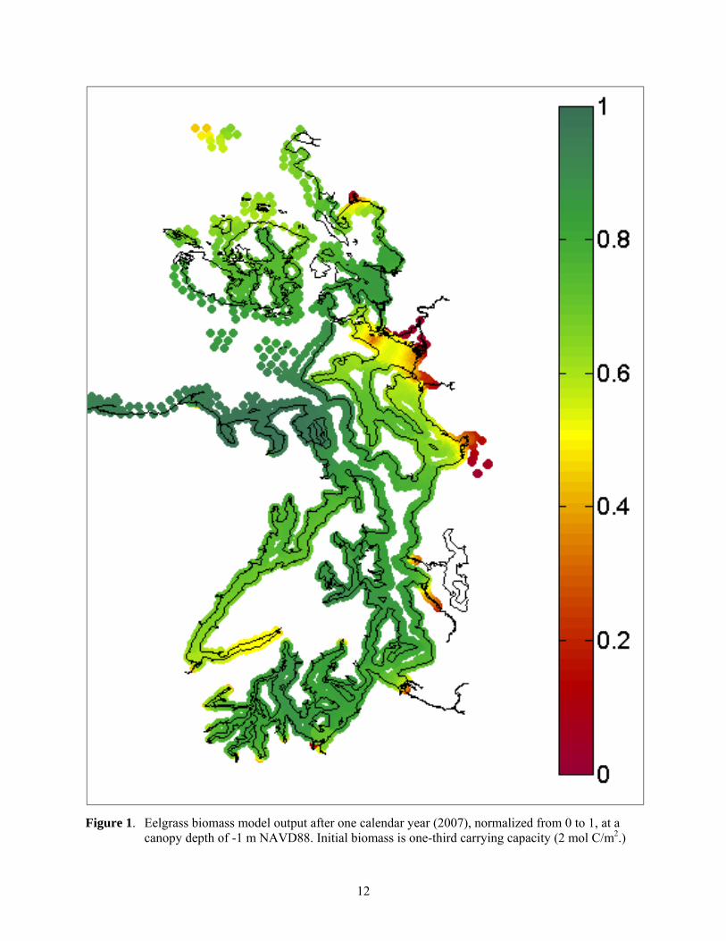
Model output at specific depths shows the broad effects of light availability, temperature, and salinity on eelgrass growth throughout Puget Sound (Figure 1 and Figure 2). At -1 m NAVD88, light is rarely limiting and eelgrass production is controlled by low salinity (e.g., in large river deltas, primarily in eastern Puget Sound) and higher temperatures (e.g., south Hood Canal). At -5 m NAVD88, production is driven most strongly by light, with areas prone to high turbidity due to sediment runoff (e.g., Skagit Bay, the Nisqually delta) or low circulation (South Sound, South Hood Canal) having notably reduced eelgrass production. The co-occurrence of stressors in some locations (e.g., those with reduced water circulation and near deltas) causes low suitability at both depths. At -5 m NAVD88, areas unsuitable at shallow depths remain so and areas with high turbidity become less suitable. Note that while model results indicate predicted growth for eelgrass below carrying capacity, the relative ranking of sites is not sensitive to initial conditions.

12

Figure 1. Eelgrass biomass model output after one calendar year (2007), normalized from 0 to 1, at a canopy depth of -1 m NAVD88. Initial biomass is one-third carrying capacity (2 mol C/m2.)

13

Figure 2. Eelgrass biomass model output after one calendar year (2007), normalized from 0 to 1, at a canopy depth of -5 m NAVD88. Initial biomass is one-third carrying capacity (2 mol C/m2.)

14

3.1.2 Spatial Analysis

The presence-absence data for eelgrass obtained from the SVMP, ShoreZone Inventory, and site visits are shown in Figure 3. Note that sites are coded as having eelgrass present or absent if eelgrass is present anywhere in the site (SVMP), and that presence includes patchy or sparse distributions (i.e., marginal habitat) as well as healthy, high-density eelgrass meadows (ShoreZone Inventory).

Of the sites that had eelgrass documented as present (1,644 sites), 17 percent had a model value (EBM) greater than 2.1 and 59 percent had a EBM value greater than 2.0. Conversely, of the sites where eelgrass was documented as absent, 53 percent had an EBM value greater than 2.0.

A histogram of EBM scores for sites with no eelgrass present indicates that on the order of 500 sites show potential to support eelgrass (i.e., EBM scores ≥2.0; Figure 4). A histogram of the ERP scores from the 2,630 sites with bathymetry data is shown in Figure 5. The vast majority (i.e., approximately 98 percent) of the sites have a low (i.e., <200) ERP score. That is, 2,587 of the sites are both small and have a relatively low EBM score. The remaining 43 sites (i.e., approximately 2 percent) have a moderate to high score.

Using only the 993 sites where eelgrass was not currently present (Figure 6), we plotted the EBM scores against bathymetry area to locate sites that were both large and predicted to have high suitability. We divided the sites into small (<10 ha), medium (10 to 50 ha) and large (>50 ha). Sites larger than 150 ha are not shown. Seven >50-ha sites had EBM scores greater than or equal to 2.0. Hundreds 10- to 50-ha sites had EBM scores greater than or equal to 2.0.

For sites without eelgrass present, we plotted the proportion of shoreline with overwater structures against the EBM scores. Figure 6 shows that about 17 sites with no eelgrass present have 10 to 50 percent of the shoreline containing overwater structures, but are otherwise predicted to be highly suitable for eelgrass (i.e., EBM ≥2.1).

Similarly, we plotted the proportion of shoreline with armoring against the EBM scores (Figure 8). The sites with EBM scores >2.1 are distributed fairly evenly across the range of proportion of armored shoreline, which suggests that the potential effects of armoring may be relevant across a range of otherwise suitable sites.

The area suitable for eelgrass varies by region (Table 2). A total of 26,576 ha showed moderate to high ECI scores. Central Puget Sound contained the greatest proportion of this area (31.6 percent) followed by North Sound (24.8 percent), San Juan Islands and Strait (23.4 percent), South Sound (9.2 percent), and Hood Canal (7.3 percent).

In Table 3, we summarize statistics on potential eelgrass area. Information is divided into four bins (i.e., unsuitable, low, moderate, and high) based on ECI scores and the area associated with each of those bins is calculated for sites within specific area ranges. For each ECI bin, an estimate is provided for current eelgrass population, historical eelgrass population, and the likelihood that eelgrass may be restored based on survey results from local planners and scientists. A total of 3,000 ha (75 percent of the 4,000-ha goal) presently without eelgrass has a high ECI value of >2.1. An additional 4,401 ha currently without eelgrass falls in the moderate ECI category. The stakeholder survey indicated that 1,275 ha within the high ECI bin appeared to be suitable for eelgrass if some actions are taken to reduce stressors.

15

Figure 3. Current eelgrass presence/absence as derived from the Submerged Vegetation Monitoring Program, the Shorezone Inventory, and site visits conducted for this project.

16

Figure 4. Histogram of EBM values for sites without eelgrass currently present.

Figure 5. Count of ERP scores, indicating low, moderate, and high scores.

17

Figure 6. Plot of EBM versus bathymetry area for 993 sites containing no present eelgrass. The seven sites greater than 50 ha and with EBM scores of >2.1 represent larger sites with a relatively high potential for restoration. One 257-ha site with an EBM score ≥2.0 is not shown. Four >200-ha sites with EBM scores <2.0 are not shown.

18

Figure 7. Plot of EBM for areas with no present eelgrass versus proportion of the site with overwater structures. Sites with EBM scores >2.0 represent potentially good sites for restoration, especially if the overwater structures are removed or improved to reduce shading. A total of 17 sites with the best growth conditions are indicated with scores >2.1.

19

Figure 8. Plot of EBM for areas with no present eelgrass versus proportion of the site with shoreline armoring. Sites with EBM scores >2.0 represent potentially good sites for restoration, especially if the armoring is removed or the armoring is presently not disturbing potential eelgrass areas. Sites with the best growth conditions are indicated with scores >2.1.

Table 2. Summary statistics by Puget Sound region for the total bathymetric area covered within each category range of ECI score.

Region

Environmental Condition Index

0 (not suitable)

<1.9 (low)

1.9 to 2.1 (moderate)

>2.1 (high)

Central (cps) 210 1,936 4,888 3,519

Hood Canal (hdc) 150 782 1,939

North (nps) 145 1,977 5,728 1,832

San Juan Islands and Strait (sjs) 1,443 3,940 1,701 4,511

South (sps) 0 567 2,458 0

1.7

1.8

1.9

2

2.1

2.2

2.3

0 0.2 0.4 0.6 0.8 1

EB

M (

mo

lC m

-2)

Armoring (Proportion)

20

Table 3. Summary statistics for the total bathymetric area covered within each category range of ECI score. Historical eelgrass area in this table was estimated using the total appropriate depth range for a site that had eelgrass present anywhere within it. This is likely an overestimation; however, not all areas were covered by historical surveys. The survey potential is based on evaluations from the stakeholder survey for specific areas. Not all areas in Puget Sound were represented in the survey results. Total absent eelgrass is the total bathymetric area where eelgrass absence was noted using all data sources including the stakeholder survey.

Environmental Condition Index

Total Area (ha)

0 (not suitable)

<1.9 (low)

1.9 to 2.1 (moderate)

>2.1 (high)

0.1 – 9.9 ha 600 1,997 3,912 1,244 7,753

10.0 – 50.0 ha 1,178 4,147 7,978 4,571 17,874

>50 ha 176 12,440 11,034 4,046 27,696

Total ha 1,954 18,584 22,924 9,861 53,323

Present Eelgrass (ha) 672 16,024 18,523 6,862 42,081

Absent Eelgrass (ha) 1,282 2,560 4,401 3,000 11,243

Historical Eelgrass (ha) 352 13,125 15,464 5,593 34,534

Overwater Structures (average % area) 1.6 1.1 0.3 0.3 n/a

Armored Shoreline (average % shoreline) 14 23 31 32 n/a

Survey Potential (ha) 48 3,199 3,280 1,275 7,802

Total Absent Eelgrass (ha) 1,287 5,250 7,380 4,031 17,949

A map of ERP (Figure 9) illustrates the location of potential restoration sites where eelgrass was not currently present, including the areas identified in the stakeholder survey; those with highest potential are shown in purple followed by green. The bathymetric area associated with the sites with an ERP >200 is greater than 100 ha per site for a total potential area of 4,492 ha. This is likely an overestimate because sometimes general areas were identified in the survey and they may not be completely devoid of eelgrass. Of the 67 sites with an ERP between 60 and 200, 31 sites (between 28 and 63 ha) have an ECI greater than 2.1, for an additional 1,215 ha of potential restoration area.

21

Figure 9. Eelgrass restoration potential (ERP: Environmental Condition x Area). Areas shown are those that currently have no eelgrass present. Note that spatial extent of the map limits resolution at fine scales.

22


The survey was sent to 1,000 stakeholders and we received 147 responses (i.e., a 14.7 percent response rate). The affiliations of respondents who left contact information (46 percent of respondents) included: U.S. Environmental Protection Agency (EPA) (2), NOAA (3), U.S. Army Corps of Engineers (1), U.S. Fish and Wildlife Service (1), Washington State Department of Transportation (1), WDFW (5), DNR (5), Ecology (3), Puget Sound Partnership (1), tribes (4), county (1), consultants (6), shellfish growers (3), universities (4), citizen groups (2), and other (25). Half of these respondents (50 percent) categorized themselves as Natural Resource Managers, Marine Biologists, and/or Nearshore/Estuarine Scientists.

Over 80 percent of respondents considered themselves to have a “good” or “excellent” understanding of the functions and values of eelgrass, its abundance and distribution throughout Puget Sound, and the stressors that affect it. Dredging and filling, shoreline development, and water quality were identified as having a large impact on eelgrass at discrete locations in Puget Sound, as well as in Puget Sound as a whole. A total of 78 percent of respondents indicated that changing policies that protect eelgrass from direct impacts (e.g., dredging, overwater structures, and mooring buoys) would enhance eelgrass in Puget Sound. A total of 90 percent of respondents indicated that changing policies that protect eelgrass from degraded environmental conditions (e.g., poor water quality and nutrient loading) would enhance eelgrass in Puget Sound. A total of 75 percent of respondents indicated that changing policies that require greater project compliance (e.g., larger mitigation ratios and higher transplant criteria) would enhance eelgrass in Puget Sound.

The areas that survey respondents identified as having lost historically present eelgrass are shown in Figure 10. These areas are distributed around Puget Sound, and are mostly found in areas where circulation is reduced and, therefore, water quality and turbidity may be stressors on eelgrass populations.

23

Figure 10. Stakeholder survey results indicating areas where respondents identified absence of eelgrass that existed previously. Note that spatial extent of the map limits resolution at fine scales.

24

3.3 Field Evaluation of Potential Sites

3.3.1 Quantitative Surveys of the Test Plots

The survival of transplanted shoots as observed during the spring quantitative surveys is summarized in Table 4. Of the nine plots planted, five (i.e., Anderson, Liberty, and Westcott deep) had eelgrass mortality rates greater than 90 percent and are, therefore, not good candidates for large-scale planting. The two sites at Joemma State Park had excellent survival rates with more shoots present in 2014 than planted in 2013. Zangle Cove and Westcott middle had some mortality, which is expected with the first year of this type of transplanting (e.g., Vavrinec et al. 2007), but did well enough to warrant further investigation for large-scale restoration. Site-specific observations are given in the following sections.

Table 4. Summary of survival at all the test planting plots and recommendations regarding future restoration.

Site Shoots planted

Area planted

(m2) Shoots counted

Survival (%)

Ave end density

(shoots/m2) Recommendation

Joemma State Park deep 712 36 930 130.6 25.83 Larger planting

Joemma State Park shallow 712 36 775 108.8 21.53 Larger planting

Zangle Cove 872 45 539 61.8 11.98 Targeted planting

Westcott middle bay 472 25 81 17.2 3.24 Trial planting

Anderson Is. deep 720 36 14 1.9 0.39 Do not plant

Anderson Is. shallow 720 36 11 1.5 0.31 Do not plant

Liberty Bay (NW site) 600 30 8 1.3 0.27 Do not plant

Liberty Bay (SE site) 720 36 3 0.4 0.08 Do not plant

Westcott head of bay 448 25 0 0.0 0.00 Do not plant

South Sound: Both test plots at Anderson Island were largely devoid of eelgrass, with a few, very small, shoots. Significant eelgrass was present at both Joemma State Park plots, with survival ranging from 50 to 300 percent. Eelgrass decreased at Zangle Cove but mortality was less than 40 percent and remaining plants looked healthy. Success roughly correlated with the coarseness of sediment at these sites and presence of currents, with successful sites having less suspended sediment when disturbed. The Zangle Cove plot was on the edge of a sandy alluvial fan, so other parts of the cove may not be as suitable for eelgrass.

Liberty Bay: While the northwest test plot was doing well in October during the qualitative survey, both sites had lost most of the transplanted eelgrass when surveyed in the spring. Nothing was obvious during the surveys to explain this high mortality.

Westcott Bay: The head of the bay site had complete eelgrass mortality before the end of the summer and, therefore, does not appear to be suitable for eelgrass at this time. The sediment was much finer, appeared to be anoxic, and had high biological disturbance from shrimp and crabs. The middle of the bay site had better survival although the overall mortality was still greater than 80 percent. Some eelgrass was found at each depth. The sediment was more coarse at this site than at the head of the bay, and while there

25

appeared to be less frequent biological disturbance, the magnitude may have been greater (e.g., larger crabs and much larger burrow mounds).

3.4 Water Properties

3.4.1 Light

The light sensor data exhibited responses to fouling over time, exposure to air, and seasonal changes of light availability (Figure 11). The most useable data collected was shortly after the sensors were installed or shortly after they were cleaned. We calculated mean daily attenuation for the South Sound and Westcott Bay the day after sensors were installed or cleaned (Figure 12). A 7-day average was also calculated for the following week to account for any temporal variation while sensors were still relatively clean. The average South Sound attenuation coefficient for the days immediately following installation and three cleanings was 0.71 m-1. The averaged attenuation for the week following each of those dates was 0.64 m-1. The average attenuation at Westcott Bay (0.99 m-1) was higher than South Sound but only two dates were included (i.e., date of installation and one date of cleaning in October). The average for the week following those two dates was 0.89 m-1 at Westcott Bay.

Figure 11. Daily PAR averaged between 10:00 a.m. and 2:00 p.m. for Westcott Bay and Anderson Island between June and December 2013. The dashed line marks 300 µmol/m2/sec, though to be the minimum light requirement for long-term maintenance of eelgrass (Thom et al. 2008).

26

Figure 12. Comparison of average daily attenuation coefficients calculated when sensors were installed or cleaned, and calculated one week after placement. Error bars are 95% C.I.

3.4.2 Temperature

Figure 13 provides temperature plots for Westcott Bay, Anderson, and Joemma State Park. The positive and negative spikes in temperature seen at Anderson and Joemma State Park for the shallow sites coincide with tides and likely reflect air temperature when sensors were exposed to air or were very shallowly submerged. With the exception of those cases, temperature varied more widely at Westcott than the other sites with the inner site showing consistent temperature above 15oC in summer. Warm periods were followed by much cooler periods at Westcott. Anderson and Joemma State Park showed less variability than Westcott during summer and were slightly warmer in fall and winter.

27

Figure 13. Daily temperature data at eelgrass canopy depth from selected eelgrass test planting locations in Puget Sound (Westcott Bay –top, Anderson Bay – mid, Joemma State Park (lower).

‐5

0

5

10

15

20

25

30

May‐13 Jun‐13 Jul‐13 Aug‐13 Sep‐13 Oct‐13 Nov‐13 Dec‐13 Jan‐14 Feb‐14 Mar‐14 Apr‐14

Temperature

°C

Anderson Shallow (‐1.0 m, MLLW) Anderson Deep (‐1.5 m, MLLW)

‐5

0

5

10

15

20

25

30

May‐13 Jun‐13 Jul‐13 Aug‐13 Sep‐13 Oct‐13 Nov‐13 Dec‐13 Jan‐14 Feb‐14 Mar‐14 Apr‐14

Temperature

°C

Joemma Shallow (‐1.0 m, MLLW) Joemma Deep (‐1.5 m, MLLW)

28

4.0 Discussion

Our primary objectives for this study were to develop and apply a range of tools to identify suitable restoration sites toward meeting the Puget Sound Partnership’s eelgrass targets, and to understand more broadly the stressors and limitations affecting eelgrass survival and recovery in Puget Sound. Avoiding damage to intact, natural seagrass systems is less expensive than trying to restore the habitat and associated food webs and processes (Cunha et al. 2014, Moberg and Rönnbäck 2003). Similarly, restoration may be inefficient or ineffective if stressors are not taken into account, and natural recruitment and expansion may be more likely to occur if stressors are reduced or removed. Seagrass restoration efforts are not always successful (Thom 1990; Orth et al. 2010; Cunha et al. 2014), but can contribute to positive gains in cover and abundance if site conditions are suitable and the restoration methods are appropriate (e.g., Thom 1990, Fonseca et al. 1998, Thom et al. 2012). To meet an ambitious goal of increasing eelgrass cover by 4,000 ha, it is likely all approaches (i.e., protection, restoration, and enhancement—including stressor abatement) will need to be applied in Puget Sound.

4.1 Modeling Suitability

Based on the modeling and substrate data, we estimate about 3,000 ha at appropriate depths is highly suitable for eelgrass but, according to available records, does not currently contain eelgrass. An additional 4,401 ha is estimated to be moderately suitable. When taking the area of sites into account, it appears that there are enough moderate to large sites with relatively high EBM scores to meet the 4,000-ha goal. However, sites smaller than 10 ha should not be excluded from consideration for restoration, because most successful eelgrass restoration projects in the region and on the west coast are generally small in area (Thom 1990; Fonseca et al. 1998). Further, strategically located but small eelgrass meadows can serve significant ecological functions for that area, and because investing resources primarily on large restoration projects can lead to significant impacts to overall success if individual projects fail, risk can be reduced by distributing restoration efforts across large and small projects.

Our spatial comparison of eelgrass model predictions with local stressors showed a number of sites predicted to be suitable that may be adversely affected by built structures. Overwater structures have a well-documented direct negative effect on eelgrass (Burdick and Short 1999; Thom et al. 2001). Abatement of shading associated with these structures should facilitate eelgrass restoration efforts at otherwise suitable sites. Similarly, shoreline armoring is present at sites that are estimated as suitable, though effects of armoring on eelgrass are unclear. For these and other potential stressors, site-specific studies are required to further evaluate suitability for eelgrass and whether stressors can be reduced or removed.

4.2 Caveats and Data Needs

We used the most current numerical models and data for circulation, water quality, and eelgrass biomass; however, significant uncertainty remains in our estimates. Most importantly, data on water clarity were sparse in nearshore areas of Puget Sound, and modeling all components of total suspended solids, including sediment, is difficult to impractical at large scales. As light is a key driver of eelgrass productivity and survival, understanding water clarity at relevant locations and scales is critical for understanding the distribution of eelgrass and determining site suitability. We were limited to light data collected once a month away from shore; while this captures some of the spatial and temporal variability,

29

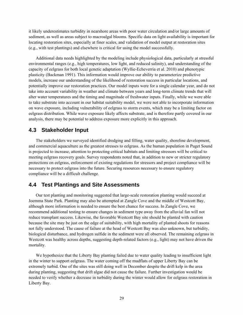
it likely underestimates turbidity in nearshore areas with poor water circulation and/or large amounts of sediment, as well as areas subject to macroalgal blooms. Specific data on light availability is important for locating restoration sites, especially at finer scales, and validation of model output at restoration sites (e.g., with test plantings) and elsewhere is critical for using the model successfully.

Additional data needs highlighted by the modeling include physiological data, particularly at stressful environmental ranges (e.g., high temperatures, low light, and reduced salinity), and understanding of the capacity of eelgrass for both local genetic adaptation (Wyllie-Echeverria et al. 2010) and phenotypic plasticity (Backman 1991). This information would improve our ability to parameterize predictive models, increase our understanding of the likelihood of restoration success in particular locations, and potentially improve our restoration practices. Our model inputs were for a single calendar year, and do not take into account variability in weather and climate between years and long-term climate trends that will alter water temperatures and the timing and magnitude of freshwater inputs. Finally, while we were able to take substrate into account in our habitat suitability model, we were not able to incorporate information on wave exposure, including vulnerability of eelgrass to storm events, which may be a limiting factor on eelgrass distribution. While wave exposure likely affects substrate, and is therefore partly covered in our analysis, there may be potential to address exposure more explicitly in this approach.


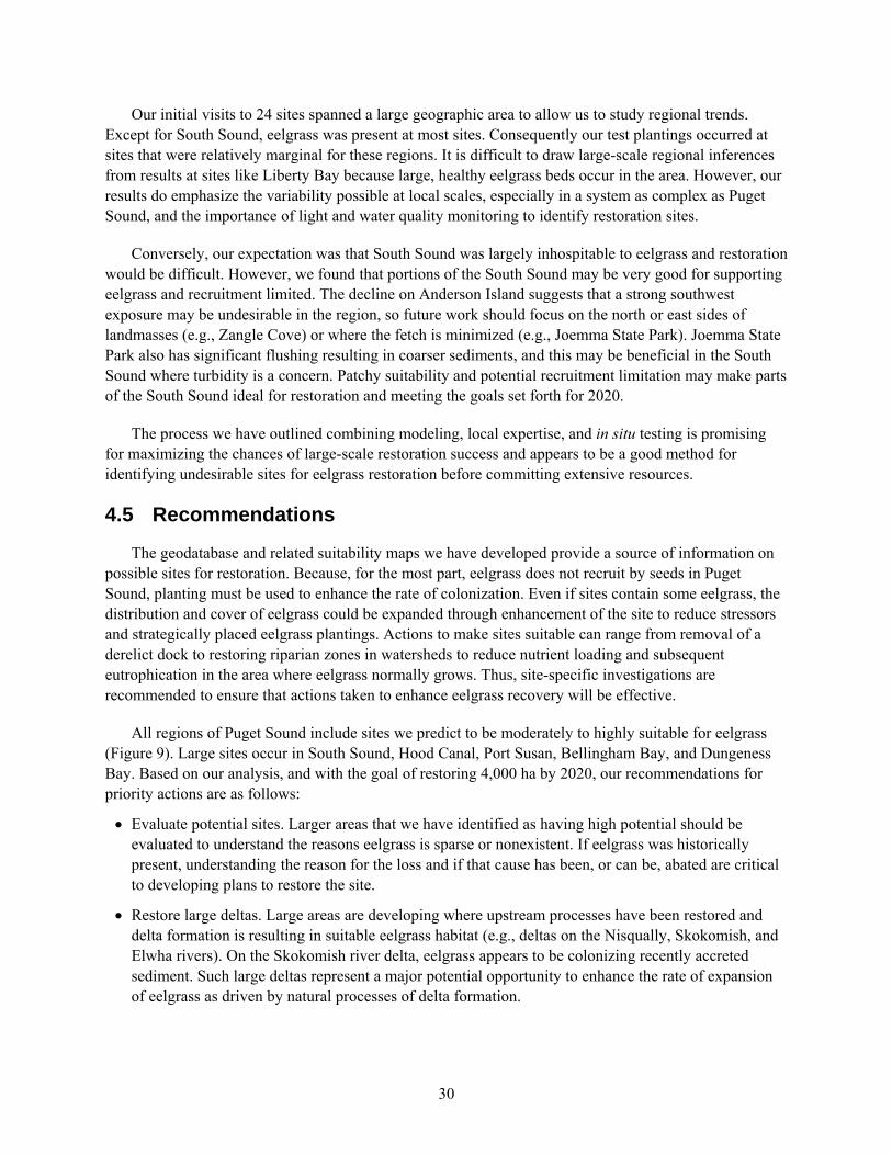
The stakeholders we surveyed identified dredging and filling, water quality, shoreline development, and commercial aquaculture as the greatest stresses to eelgrass. As the human population in Puget Sound is projected to increase, attention to protecting critical habitats and limiting stressors will be critical to meeting eelgrass recovery goals. Survey respondents noted that, in addition to new or stricter regulatory protections on eelgrass, enforcement of existing regulations for stressors and project compliance will be necessary to protect eelgrass into the future. Securing resources necessary to ensure regulatory compliance will be a difficult challenge.

4.4 Test Plantings and Site Assessments

Our test planting and monitoring suggested that large-scale restoration planting would succeed at Joemma State Park. Planting may also be attempted at Zangle Cove and the middle of Westcott Bay, although more information is needed to ensure the best chance for success. In Zangle Cove, we recommend additional testing to ensure changes in sediment type away from the alluvial fan will not reduce transplant success. Likewise, the favorable Westcott Bay site should be planted with caution because the site may be just on the edge of suitability, with high mortality of planted shoots for reasons not fully understood. The cause of failure at the head of Westcott Bay was also unknown, but turbidity, biological disturbance, and hydrogen sulfide in the sediment were all observed. The remaining eelgrass in Westcott was healthy across depths, suggesting depth-related factors (e.g., light) may not have driven the mortality.

We hypothesize that the Liberty Bay planting failed due to water quality leading to insufficient light in the winter to support eelgrass. The water coming off the mudflats of upper Liberty Bay can be extremely turbid. One of the sites was still doing well in December despite the drift kelp in the area during planting, suggesting that drift algae did not cause the failure. Further investigation would be needed to verify whether a decrease in turbidity during the winter would allow for eelgrass restoration in Liberty Bay.

30

Our initial visits to 24 sites spanned a large geographic area to allow us to study regional trends. Except for South Sound, eelgrass was present at most sites. Consequently our test plantings occurred at sites that were relatively marginal for these regions. It is difficult to draw large-scale regional inferences from results at sites like Liberty Bay because large, healthy eelgrass beds occur in the area. However, our results do emphasize the variability possible at local scales, especially in a system as complex as Puget Sound, and the importance of light and water quality monitoring to identify restoration sites.

Conversely, our expectation was that South Sound was largely inhospitable to eelgrass and restoration would be difficult. However, we found that portions of the South Sound may be very good for supporting eelgrass and recruitment limited. The decline on Anderson Island suggests that a strong southwest exposure may be undesirable in the region, so future work should focus on the north or east sides of landmasses (e.g., Zangle Cove) or where the fetch is minimized (e.g., Joemma State Park). Joemma State Park also has significant flushing resulting in coarser sediments, and this may be beneficial in the South Sound where turbidity is a concern. Patchy suitability and potential recruitment limitation may make parts of the South Sound ideal for restoration and meeting the goals set forth for 2020.

The process we have outlined combining modeling, local expertise, and in situ testing is promising for maximizing the chances of large-scale restoration success and appears to be a good method for identifying undesirable sites for eelgrass restoration before committing extensive resources.

4.5 Recommendations

The geodatabase and related suitability maps we have developed provide a source of information on possible sites for restoration. Because, for the most part, eelgrass does not recruit by seeds in Puget Sound, planting must be used to enhance the rate of colonization. Even if sites contain some eelgrass, the distribution and cover of eelgrass could be expanded through enhancement of the site to reduce stressors and strategically placed eelgrass plantings. Actions to make sites suitable can range from removal of a derelict dock to restoring riparian zones in watersheds to reduce nutrient loading and subsequent eutrophication in the area where eelgrass normally grows. Thus, site-specific investigations are recommended to ensure that actions taken to enhance eelgrass recovery will be effective.

All regions of Puget Sound include sites we predict to be moderately to highly suitable for eelgrass (Figure 9). Large sites occur in South Sound, Hood Canal, Port Susan, Bellingham Bay, and Dungeness Bay. Based on our analysis, and with the goal of restoring 4,000 ha by 2020, our recommendations for priority actions are as follows:

Evaluate potential sites. Larger areas that we have identified as having high potential should be evaluated to understand the reasons eelgrass is sparse or nonexistent. If eelgrass was historically present, understanding the reason for the loss and if that cause has been, or can be, abated are critical to developing plans to restore the site.

Restore large deltas. Large areas are developing where upstream processes have been restored and delta formation is resulting in suitable eelgrass habitat (e.g., deltas on the Nisqually, Skokomish, and Elwha rivers). On the Skokomish river delta, eelgrass appears to be colonizing recently accreted sediment. Such large deltas represent a major potential opportunity to enhance the rate of expansion of eelgrass as driven by natural processes of delta formation.

31

Improve water quality. Modeling and test planting indicate that South Sound could support more eelgrass. We are unsure why eelgrass has not colonized areas that appear suitable according to the modeling and test plantings. Water clarity may be relatively low much of the year due to algal blooms and/or suspended sediment. Further analysis of the sources of turbidity and potential methods to improve water clarity should be conducted prior to implementation of larger planting efforts. If water quality is suitable, then planting can compensate for any recruitment limitation that may exist.

Coordinate stakeholders. Local shoreline planners and other scientists who are knowledgeable about local issues can identify locations that may support eelgrass with relatively simple actions. Strategies proven to be successful (e.g., anchor out zones) can be simple and relatively easy to implement. Actions with high chances of success include removal of overwater structures and policies to limit activities that disturb eelgrass (e.g., recreational shellfish harvest, boat groundings, and boat anchors and chains).

Monitor eelgrass transplant and mitigation efforts. Long-term monitoring of eelgrass transplant projects and projects that require eelgrass mitigation will build and enhance the knowledgebase for future projects.

5.0 Conclusions

Seagrasses, including eelgrass, have been declining globally and losses have been primarily attributed to stressors resulting from anthropogenic activities (Duarte 2002; Orth et al. 2006; Short and Wyllie-Echeverria 1996; Short et al. 2011, Waycott et al. 2009). In Puget Sound, substantial losses are believed to be due to physical changes in shorelines, periodic physical disturbances, and degradation in water quality (Thom and Hallum 1990; Thom 1995; Dowty et al. 2010; Thom et al. 2011). Furthermore, climate change and human-induced disturbances are expected to increase, and may exacerbate, eelgrass loss in Puget Sound.

The development of a site-selection model not only has to consider the historical distribution of eelgrass in an area, but also stressors that limit its growth. In addition, effective regulations and stewardship of eelgrass will protect and conserve the resource through regulatory and educational means.

The purpose of this project was to develop an approach and set of tools to optimize eelgrass restoration in Puget Sound to meet the Puget Sound Partnership’s regional recovery goal of 4,000 ha by 2020—a 20 percent increase from the established baseline (PSP 2013). We integrated a set of numerical models, geospatial databases, and field studies to identify potential sites for eelgrass restoration. Input from local and regional resource managers refined model outputs to areas previously vegetated with eelgrass and that might, through stressor abatement, sustain eelgrass once again. Model performance was evaluated through the success of eelgrass test transplants at potential sites. The results of the test transplants prioritized sites for large-scale restoration and developed recommended management actions to improve site conditions for additional seagrass expansion, conservation, and protection.

Two main drivers in the development of recovery targets and priority actions to improve the Puget Sound ecosystem involved whether suitable area exists for 20 percent more eelgrass and what obstacles or barriers need to be considered. The project incorporated the best available science, along with stakeholder input, and demonstrated the potential for eelgrass restoration in Puget Sound. The model results suggest

32

ample area is available in Puget Sound for expansion of eelgrass and that 4,000 ha can be restored. However, when locating suitable sites, limitations and challenges must be considered. Project findings indicate the following constraints to eelgrass restoration:

recruitment limitation (e.g., low seed production and slow rhizome spread)

impacts to donor stocks

natural variation in ocean conditions

climate change and associated uncertainties

water clarity, including watershed influences

human disturbances on site and landscape scales

land ownership

regulatory issues (e.g., disturbances and permits)

implementation and enforcement of effective regulations for enhancing eelgrass recovery

habitat suitability model data limitations

availability and quality of nearshore data for model inputs and verification, including bathymetry, water quality and eelgrass presence, biomass, and dynamics

availability of information about local adaptation and genetic variation.

33

6.0 References

Backman TWH. 1991. “Genotypic and phenotypic variability of Zostera marina on the west coast of North America.” Canadian Journal of Botany 69:1361-1371.

Bjork M, F Short, E Mcleod, and S Beer. 2008. Managing seagrasses for resilience to climate change. IUCN, Gland Switzerland. 56 pp.

Burd AB and KH Dunton. 2001. “Field Verification of a Light-Driven Model of Biomass Changes in the Seagrass Halodule wrightii.” Marine Ecology Progress Series 209:85-98.

Burdick DM and FT Short. 1999. “The effects of boat docks on eelgrass beds in coastal waters of Massachusetts.” Environmental Management 23:231-240.

Butler RW. 1995. “The patient predator: Foraging and population ecology of the great blue heron, Ardea herodias, in British Columbia.” Occasional Papers for Canadian Wildlife Service No. 86.

Costanza R, R d’Arge, R de Groot, S Farber, M Grasso, B Hannon, K Limburg, S Naeem, RV O’Neill, J Paruelo, RG Raskin, P Sutton, and M van den Belt. 1997. “The value of the world’s ecosystem services and natural capital.” Nature 387:253-260.

Cunha AH, NN Marbá, MM van Katwijk, C Pickerell, M Henriques, G Bernard, MA Ferreira, S Garcia, JM Garmendia, and P Manent. 2014. “Changing paradigms in seagrass restoration.” Restoration Ecology 20(4):417-430.

Dennison WC, RJ Orth, KA Moore, J C Stevenson, V Carter, S Kollar, P W Bergstrom, and R A Batiuk. 1993. “Assessing water quality with submerged aquatic vegetation: habitat requirements as barometers of Chesapeake Bay health.” BioScience 43(2):86-94.

Dowty P, H Berry, and J Gaeckle. 2010. Developing indicators and targets for eelgrass in Puget Sound: A science assessment. Nearshore Habitat Program, Aquatic Resources Division, Washington Department of Natural Resources, Olympia, Washington.

Duarte CM. 2002. “The future of seagrass meadows.” Environmental Conservation 29(2):192-206.

Duarte CM and CL Chiscano. 1999. “Seagrass biomass and production: a reassessment.” Aquatic Botany 65:159-174.

Eldridge PM, JE Kaldy, and AB Burd. 2004.” Stress response model for the tropical seagrass Thalassia testudinum: the interactions of light, temperature, sedimentation, and geochemistry.” Estuaries 27:923-937.

Finlayson D.P., Haugerud R.A., Greenberg, H. and Logsdon, M.G. (2000) Puget Sound Digital Elevation Model. University of Washington, (http://students.washington.edu/dfinlays/pugetsound/)

34

Finlayson D.P. (2005) Combined bathymetry and topography of the Puget Lowland, Washington State. University of Washington, (http://www.ocean.washington.edu/data/pugetsound/)

Fonseca MS, WJ Kenworthy, and GW Thayer. 1998. Guidelines for the conservation and restoration of seagrasses in the Unites States and adjacent waters. National Oceanic and Atmospheric Administration, Coastal Ocean Office (NOAA Coast Ocean Program Decision Analysis Series No. 12), Silver Spring, Maryland.

Gaeckle J, P Dowty, H Berry, and L Ferrier. 2011. Puget Sound Submerged Vegetation Monitoring Project 2010 Report. Nearshore Habitat Program, Aquatic Resources Division, Washington Department of Natural Resources, Olympia, Washington. Accessed at http://www.dnr.wa.gov/Publications/aqr_eelgrass_svmp_report.pdf.

Green EP and FT Short. 2003. World Atlas of Seagrasses. University of California Press. Berkeley, California.

Hemminga MA and CM Duarte. 2000. Seagrass Ecology. Cambridge University Press, Cambridge. Pp. 298.

Hinrichsen D. 1999. “The coastal population explosion.” In proceedings Trends and future challenges for U.S. National Ocean and Coastal Policy, eds. Cincin-Sain B, RW Knecht, and N Foster.

Krause-Jensen D, TM Greve, and K Nielsen. 2005. “Eelgrass as a bioindicator under the European Water Framework Directive.” Water Resources Management 19(1):63-75.

Larkum AWD, RJ Orth, and CM Duarte, eds. 2006. Seagrasses: biology, ecology and conservation. Springer, Dordrecht, The Netherlands. 691 pp.

Lotze HK, HS Lenihan, BJ Bourque, RH Bradbury, RG Cooke, MC Kay, SM, Kidwell, MX Kirby, CH Peterson, and JBC Jackson. 2006. “Depletion, degradation, and recovery potential of estuaries and coastal seas.” Science 312:1806-1809.

Moberg F and P Rönnbäck. 2003. “Ecosystem services of the tropical seascape: interactions, substitutions and restoration.” Ocean and Coastal Management 46:27–46.

NOAA – National Oceanic and Atmospheric Administration. 2010. Vertical Datum Transformation: Integrating America’s Elevation Data. Accessed 2/24/2014 at vdatum.noaa.gov.

Parker B, KW Hess, DG Milbert, and S Gill. 2003. “A national vertical datum transformation tool.” Sea Technology 44(9):10-15.

Puget Sound Partnership. 2013. 2013 State of the Sound: A Biennial Report on the Recovery of Puget Sound. Tacoma, Washington. Page 177.This State of the Sound Report to the Governor and Legislature is consistent with RCW 90.71.370 (3)

Orth RJ, TJB Carruthers, WC Dennison, CM Duarte, JW Fourqurean, KL Heck, AR Hughes, GA Kendrick, WJ Kenworthy, S Olyarnik, FT Short, M Waycott, and SL Williams. 2006. “A global crisis for seagrass ecosystems.” BioScience 56:987-996.

35

Orth RJ, SR Marion, KA Moore, and DJ Wilcox. 2010. “Eelgrass (Zostera marina L.) in the Chesapeake Bay region of mid-Atlantic coast of the USA: challenges in conservation and restoration.” Estuaries and Coasts 33:139-150.

Phillips RC. 1984. The ecology of eelgrass meadows in the Pacific Northwest: a community profile. FSW/OBS-84/24, U.S. Fish and Wildlife Service. Available at http://www.nwrc.gov/library.html.

Rehr AP, GD Williams, N Tolimieri, and PS Levin. 2014. “Impacts of terrestrial and shoreline stressors on eelgrass in Puget Sound: an expert elicitation.” Coastal Management 42:246-262.

Simenstad CA. 1994. “Faunal associations and ecological interactions in seagrass communities of the Pacific Northwest coast.” In Seagrass Science and Policy in the Pacific Northwest: Proceedings of a Seminar Series, eds. Wyllie-Echeverria S, AM Olson, and MJ Hershman. EPA 910/R-94 004, U.S. Environmental Protection Agency, Seattle, Washington.

ShoreZone Inventory. 2001. The Washington State ShoreZone Inventory. Nearshore Habitat Program, Washington State Department of Natural Resources, Olympia, Washington.

Short FT and S Wyllie-Echeverria. 1996. “Natural and human induced disturbances of seagrasses.” Environmental Conservation 23:17-27.

Short FT, B Polidoro, SR Livingstone, KE Carpenter, S Bandeira, JS Bujang, HP Calumpong, TJB Carruthers, RG Coles, WC Dennison, PLA Erftemeijer, MD Fortes, AS Freeman, TG Jagtap, AHM Kamal, GA Kendrick, WJ Kenworthy, YA La Nafie, IM Nasution, RJ Orth, A Prathep, JC Sanciangco, B van Tussenbroek, SG Vergara, M Waycott, and JC Zieman. 2011. “Extinction risk assessment of the world’s seagrass species.” Biological Conservation 144:1961-1971.

Thom RM and L Hallum. 1990. Long-term changes in the areal extent of tidal marshes, eelgrass meadows and kelp forests of Puget Sound. EPA 910/9-91-005, Final Report to Office of PS, Region 10, U.S. Environmental Protection Agency.

Thom RM, AB Borde, GD Williams, JA Southard, SL Blanton, and DL Woodruff. 2001. “Effects of multiple stressors on eelgrass restoration projects.” In Proceedings of Puget Sound Research 2001, the fifth Puget Sound Research Conference, Vol. 1, ed. T Droscher. Puget Sound Water Quality Authority, Olympia, Washington.

Thom RM, KE Buenau, C Judd, and VI Cullinan. 2011. Eelgrass (Zostera marina L.) stressors in Puget Sound. PNWD-20508, Battelle−Pacific Northwest Division, Richland, Washington.

Thom RM, SL Southard, AB Borde, and P Stoltz. 2008. “Light requirements for growth and survival of eelgrass (Zostera marina L.) in Pacific Northwest (USA) estuaries.” Estuaries and Coasts 31:969-980.

Thom RM. 1990. “A review of eelgrass (Zostera marina L.) transplanting projects in the Pacific Northwest.” The Northwest Environmental Journal 6:121-137.

Thom RM. 1995. “Implications for restoration: light, temperature, and enriched CO2 effects on eelgrass (Zostera marina L.).” In Proceedings of Puget Sound Research ‘95: Puget Sound Water Quality Authority, Olympia, Washington.

36

Thom, RM, HL Diefenderfer, J Vavrinec, and AB Borde. 2012. “Restoring resiliency: case studies from Pacific Northwest estuarine eelgrass (Zostera marina L.) ecosystems.” Estuaries and Coasts 78:78-91.

Vavrinec, III J, RM Thom, JA Southard, AB Borde, SS Southard, and J Cordell. 2007. Habitat mitigation monitoring at the Clinton ferry terminal, Whidbey Island. Annual Report Number 10 Covering the Period of December 2005 − November 2006. PNWD-3822, Battelle−Pacific Northwest Division, Richland, Washington.

Vavrinec, III J. AB Borde, RM Thom, SL Southard, J Elster, KD Hall, LM Aston, and JL Gaeckle. 2014. Evaluation of potential eelgrass restoration sties: methods, results, and recommendations. PNNL-23502.

Waycott M, CM Duarte, TJB Carruthers, RJ Orth, WC Dennison, S Olyanik, A Calladine, JW Fourqurean, KL Heck Jr., AR Hughes, GA Kendrick, WJ Kenworthy, FT Short, and SL Williams. 2009. “Accelerating loss of seagrasses across the globe threatens coastal ecosystems.” Proceedings of the National Academy of Sciences 106:12377-12381.

Wyllie-Echeverria S, SL Talbot, and JR Rearick. 2010. “Genetic structure and diversity of Zostera marina (eelgrass in the San Juan Archipelago, Washington, USA.” Coasts and Estuaries 33:811-827

DNR (Washington State Department of Natural Resources). 2014. Submerged Vegetation Monitoring Program: Geospatial Database User Manual. Nearshore Habitat Program. Aquatic Resources Division, Washington Department of Natural Resources, Olympia, Washington.

Wilson UW and JB Atkinson. 1995. “Black brant winter and spring-stages use at two Washington coastal areas in relation to eelgrass abundance.” The Condor 97:91-98.

Yang Z and T Khangaonkar. 2010. “Multi-scale modeling of Puget Sound using an unstructured-grid coastal ocean model: from tide flats to estuaries and coastal waters.” Ocean Dynamics 60:1621-1637.

Appendix A

Geodatabase Structure

A.1

Appendix A

Geodatabase Structure

Table A.1. The contents of the Eelgrass Restoration Site Prioritization Geodatabase. All data files are products of intersection of the source feature classes with the Submerged Vegetation Monitoring Program (SVMP) site assessment units (WADNR 2014).

Name Type Source Description

Sites_eg_restoration_potential

polygon feature class

PNNL 2014 All attributes that were used to determine eelgrass restoration site potential.

Sites_eg_biomass_model_output*


PNNL 2014 Potential biomass applied to depth polygons. Biomass values range: 0 to 2.3 mol C/m2. 2 mol C/m2 = model start value. Values >2 indicate growth in 1-year model run.

Sites_current_eg_presence


PNNL 2013 (23 sites) DNR 2000-12 (383 sites)

Binary presence or absence. Presence if observations from either source occurred in the assessment unit.

Sites_shorezone_ln Line feature class

ShoreZone Inventory 2001

Binary presence or absence. Presence if any of the line occurred in the assessment unit and site was not sampled by either of the above sources (DNR and PNNL). Substrate: Proportion of each assessment unit (length) with suitable substrate.

Sites_shorezone_eg_presence_poly


ShoreZone Inventory 2001

Binary presence or absence of eelgrass. Presence if of the polygon occurred in the assessment unit and site was not sampled by either of the above sources.

Sites_historical_eg_presence


Thom and Hallum 1990 digitized by Jeremy Davies, NOAA 2009

Binary presence or absence. Presence if historical eelgrass polygon was present in the assessment unit.

Sites_overwater_structures


PSNERP 2009 Proportion of assessment unit (area) with overwater structure.

Sites_shoreline_armoring

line feature class PSNERP 2009 Proportion of assessment unit (length) armored.

DRN = Washington State Department of Natural Resources; NOAA = National Oceanic and Atmospheric Administration; PNNL = Pacific Northwest National Laboratory; PSNERP = Puget Sound Nearshore Ecosystem Restoration Project.

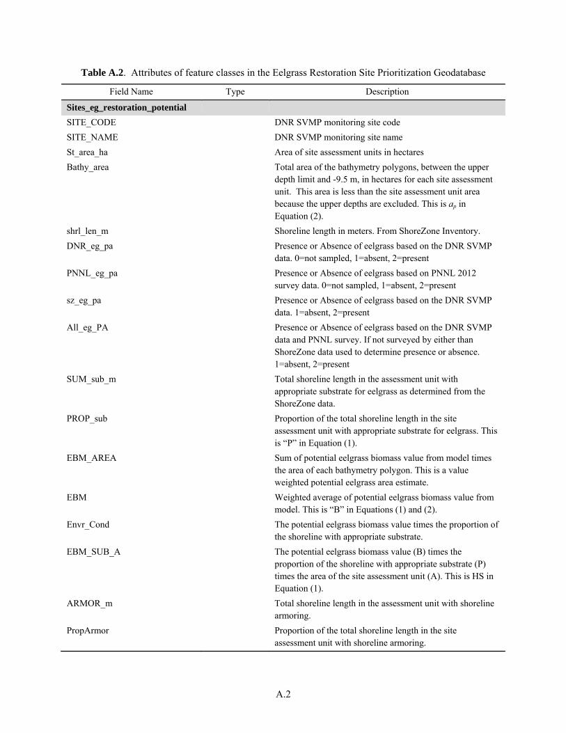
A.2

Table A.2. Attributes of feature classes in the Eelgrass Restoration Site Prioritization Geodatabase

Field Name Type Description

Sites_eg_restoration_potential

SITE_CODE DNR SVMP monitoring site code

SITE_NAME DNR SVMP monitoring site name

St_area_ha Area of site assessment units in hectares

Bathy_area Total area of the bathymetry polygons, between the upper depth limit and -9.5 m, in hectares for each site assessment unit. This area is less than the site assessment unit area because the upper depths are excluded. This is ap in Equation (2).

shrl_len_m Shoreline length in meters. From ShoreZone Inventory.

DNR_eg_pa Presence or Absence of eelgrass based on the DNR SVMP data. 0=not sampled, 1=absent, 2=present

PNNL_eg_pa Presence or Absence of eelgrass based on PNNL 2012 survey data. 0=not sampled, 1=absent, 2=present

sz_eg_pa Presence or Absence of eelgrass based on the DNR SVMP data. 1=absent, 2=present

All_eg_PA Presence or Absence of eelgrass based on the DNR SVMP data and PNNL survey. If not surveyed by either than ShoreZone data used to determine presence or absence. 1=absent, 2=present

SUM_sub_m Total shoreline length in the assessment unit with appropriate substrate for eelgrass as determined from the ShoreZone data.

PROP_sub Proportion of the total shoreline length in the site assessment unit with appropriate substrate for eelgrass. This is “P” in Equation (1).

EBM_AREA Sum of potential eelgrass biomass value from model times the area of each bathymetry polygon. This is a value weighted potential eelgrass area estimate.

EBM Weighted average of potential eelgrass biomass value from model. This is “B” in Equations (1) and (2).

Envr_Cond The potential eelgrass biomass value times the proportion of the shoreline with appropriate substrate.

EBM_SUB_A The potential eelgrass biomass value (B) times the proportion of the shoreline with appropriate substrate (P) times the area of the site assessment unit (A). This is HS in Equation (1).

ARMOR_m Total shoreline length in the assessment unit with shoreline armoring.

PropArmor Proportion of the total shoreline length in the site assessment unit with shoreline armoring.

A.3

Table A.2. (contd)


Prop_OWS Proportion of the site assessment unit with overwater structures.

EG_hist Estimated historical eelgrass presence. 0=absence, 1=presence.

Sites_eg_biomass_model_output

SITE_CODE Text code associated with the site polygon as determined by DNR

SITE_NAME Text long name of site polygon as determined by DNR

UDL_mNAVD8 Float upper depth limit elevation of eelgrass in meters relative to NAVD88

Bathy_m Float bathymetry elevation in meters relative to NAVD88

DepthBin Short eelgrass model depth bin relative to EBM

EBM Double eelgrass biomass model output value (mol C/m^^2)

Shape_Length Double GIS autogenerated polygon length value in meters

Shape_Area Double GIS autogenerated polygon area in square meters

Sites_historical_eelgrass_presence

Site Code Text code associated with the site polygon as determined by DNR


OBJECTID Long Index value from Historic_PS_Eelgrass_Dist_From_Thom_v2 shapefile



Sites_overwater_structures



OBJECTID Long OBJECTID

SUBBASIN Text SUBBASIN

Stucture_ Text short description of type of structure



Sites_shoreline_armoring



OBJECTID_1 Long Index value from PSARMORt (original data set), equivalent valueis OBJECTID

SUBBASIN Text short regional descriptor

A.4

Table A.2. (contd)


Armor_YN Text Y = armoring present


Sites_shorezone_eg_presence_poly



UNIT_ID Long Index value from eelgrass ShoreZone Inventory theme

EELGRASS Text Quaternary indicator of eelgrass status, ABSENT, PATCHY, CONTINUOUS, NO DATA

eelsub_area_ha Double area of eelgrass/substrate area in hectares

eel_pa Short Binary indication or eelgrass presence/absence where 1 = presence



Sites_shorezone_ln



UNIT_ID Long Index value from eelgrass ShoreZone Inventory theme

EELGRASS Text Quaternary indicator of eelgrass status, ABSENT, PATCHY, CONTINUOUS, NO DATA

ZoneComp Text shorezone tidal zone value from ShoreZone Inventory

Material Text substrate material components from sz inventory

Good_sed Short Binary indicator of good substrate where 1 = good substrate

eelsub_len_m Double length of eelgrass zone within the assessment unit

eel_pa Short Binary indication or eelgrass presence/absence where 1 = presence


EBM = biomass productivity potential; DRN = Washington State Department of Natural Resources; GIS = geographic information system; NAVD88 = North American Vertical Datum of 1988; NOAA = National Oceanic and Atmospheric Administration; PNNL = Pacific Northwest National Laboratory; PSNERP = Puget Sound Nearshore Ecosystem Restoration Project.

PNNL-23635

Distribution

No. of No. of Copies Copies

Distr.1

# Name Organization Address City, State and ZIP Code

# Organization Address City, State and ZIP Code Name Name Name Name Name (#)

# Name Organization Address City, State and ZIP Code

# Foreign Distribution # Name

Organization Address Address line 2 COUNTRY

# Local Distribution Pacific Northwest National Laboratory Name Mailstop Name Mailstop Name Mailstop Name Mailstop Name (PDF)

Eelgrass (Zostera marina L. Restoration in Puget … (Zostera marina L.) Restoration in Puget ......

Documents

Transcript of Eelgrass (Zostera marina L. Restoration in Puget … (Zostera marina L.) Restoration in Puget ......