EELECTROSTATICS WITHLECTROSTATICS WITH...

EELECTROSTATICS WITHLECTROSTATICS WITHMATLABMATLAB

A MATLAB Computer SupplementTo ENEE 380

Spring Semester 1999University of Maryland at College Park

Eric Dunn

Table of Contents

TABLE OF CONTENTS .................................................................................................................................... 2

INTRODUCTION................................................................................................................................................ 3

GETTING STARTED......................................................................................................................................... 4

VECTOR BASICS ............................................................................................................................................... 7

DECLARING A VECTOR....................................................................................................................................... 7VECTOR ALGEBRA.............................................................................................................................................. 8ORTHOGONAL COORDINATE SYSTEMS.............................................................................................................. 9FIELD ANALYSIS............................................................................................................................................... 10SAMPLE PROBLEMS .......................................................................................................................................... 12

VECTOR CALCULUS ..................................................................................................................................... 14

GRADIENT......................................................................................................................................................... 14DIVERGENCE..................................................................................................................................................... 15CURL ................................................................................................................................................................. 17SCALAR LINE INTEGRAL .................................................................................................................................. 18VECTOR LINE INTEGRAL .................................................................................................................................. 19FLUX (SURFACE) INTEGRAL............................................................................................................................. 20SAMPLE PROBLEMS .......................................................................................................................................... 22

ELECTROSTATICS SIMULATORS ............................................................................................................ 24

DISCRETE ELECTROSTATICS PLOTTER............................................................................................................. 24LAPLACIAN SOLVER ......................................................................................................................................... 25SAMPLE PROBLEMS .......................................................................................................................................... 26

SOURCE CODES .............................................................................................................................................. 27

ANIMLAPLACE.M .............................................................................................................................................. 27CURL.M.............................................................................................................................................................. 27DIVERGENCE.M ................................................................................................................................................. 31ELECT.M ............................................................................................................................................................ 34FLUXINT.M ........................................................................................................................................................ 36GRAD.M ............................................................................................................................................................. 40LAPLACE.M........................................................................................................................................................ 41LINEINTS.M........................................................................................................................................................ 44LINEINTV.M....................................................................................................................................................... 47SHOW.M............................................................................................................................................................. 51START.M............................................................................................................................................................ 51VALUE.M ........................................................................................................................................................... 52

Introduction

This course packet is intended to serve as a supplement to the introductory electrostaticscourse ENEE 380. It focuses on using MATLAB as a complement to analyzingelectromagnetic problems and as a tool to help visualize multidimensional fields.

I emphasize the word supplement because the best way for a student to learn any newconcept is not to rely on one text book or one software package, but to supplementwhatever they are provided with by doing exploration and research on their own. In thecase of MATLAB, the best way to learn how to apply it to electrostatic theory is to justsit down at the PC and play. Type "help command" to find reference on new commandsand how to code them. Take concepts you learn in class and see if you can recreate themin MATLAB. Work through this packet of materials and invent your own problems andwrite your own software packages.

In my experience, this is the best way to learn and remember theory taught in class.Many of the concepts that students learn in ENEE 380 are not new to them. Most of thetheories were introduced in a physics survey course and most of the mathematics werelearned in a vector calculus course. The difficulty comes in combining these two areas.

When I took MATH 241 (vector calculus), the class had a Mathematica supplement.Working with this computer software package helped me and my classmates to betterunderstand the concepts we were learning. This experience has served as my motivationfor writing this course supplement.

This course packet assumes that the student has some understanding of MATLAB syntaxand programming. If the student is familiar with C programming, then this will helpthem in understanding some of the source codes. If the student has never used MATLABbefore, then there are numerous excellent introductory books available.

Source codes for all of the files are included in the Appendix of this packet. The studentis encouraged to read through them and make modifications to improve the applications.To receive the actual files, contact your professor.

Lastly, I would like to say that I'm an electrical engineer, not a computer scientist. A lotof the codes I wrote are probably not written in the most efficient way. There are manyparts where I coded "by force" to overcome the fact that MATLAB is a numericalanalysis package and doesn't handle symbolic expressions like Mathematica. However,in doing so, it forced me to have a better understanding of the concepts.

Getting Started

The following files were compiled for MATLAB version 5.1 and are used in this coursepacket:

PROGRAM FILESM-File Bytes

animlaplace.m 700curl.m 14,860

divergence.m 15,048elect.m 7,173fluxint 14,926grad.m 7,281

laplace.m 10,885lineints.m 14,969lineintv.m 15,571show.m 183start.m 549value.m 1,223

vector*.m -

ANIMATION FILES(USED TO CREATE *.MAT)

M-File Bytesaddition.m 2,699curl1.m 3,170curl2.m 3,154curl3.m 3,183div1.m 1,481div2.m 1,480div3.m 1,590

scalar.m 2,535

MAT-FILES(BECAUSE OF SIZE, THESE ARE ZIPPED SEPEARATELY)

MAT-File Bytesadd.mat 6,516,232cur1.mat 2,576,296cur2.mat 2,424,760cur3.mat 5,000,872diver1.mat 2,121,688diver2.mat 2,121,688diver3.mat 9,243,880dotp.mat 2,243,880rotat.mat 3,788,584

GIF-FILES(ANIMATIONS CREATED WITH PAINT SHOP PRO)

File Size 14.4 KDownload

28.8 KDownload

56 KDownload

ISDNDownload

addition.gif 21 Kb 16 sec 8 sec 4 sec 2 seccurl1.gif 8.1 Kb 7 sec 4 sec 2 sec <1 seccurl2.gif 7.5 Kb 6 sec 3 sec 2 sec <1 seccurl3.gif 12 Kb 9 sec 5 sec 3 sec <1 secdiv1.gif 5.0 Kb 4 sec 2 sec <1 sec <1 secdiv2.gif 5.5 Kb 5 sec 3 sec 2 sec <1 secdiv3.gif 7.2 Kb 6 sec 3 sec 2 sec <1 sec

laplace.gif 175 Kb 2 min 9 sec 1 min 4 sec 34 sec 15 secscalar.gif 5.3 Kb 4 sec 2 sec 2 sec <1 sec

(Download times are provided because they were used in creation of course web-page)

All of the files need to be copied into your MATLAB working directory.To view the animations, at the MATLAB prompt simply type:

show('filename')

To launch the package of programs, at the MATLAB prompt type:

start

The following screen should open from which you can select which program you wouldlike to run.

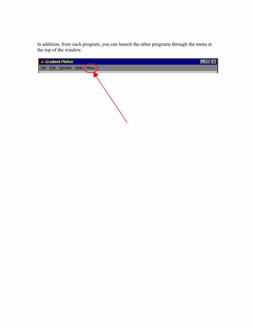
In addition, from each program, you can launch the other programs through the menu atthe top of the window.

Vector Basics

Declaring a Vector

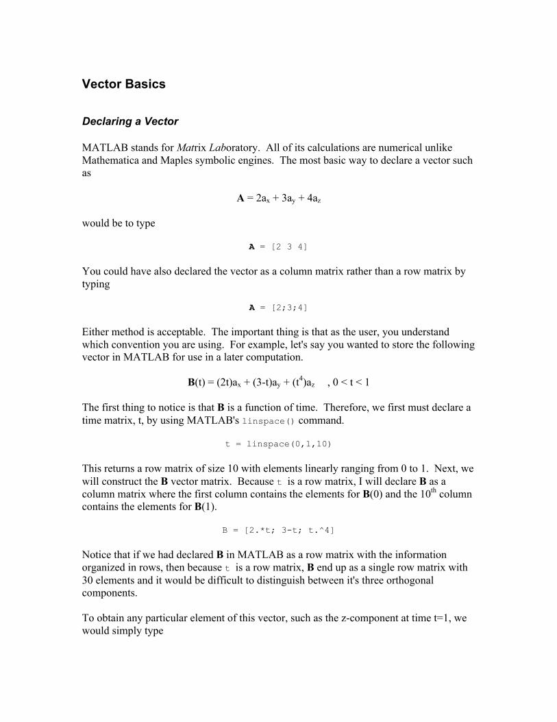
MATLAB stands for Matrix Laboratory. All of its calculations are numerical unlikeMathematica and Maples symbolic engines. The most basic way to declare a vector suchas

A = 2ax + 3ay + 4az

would be to type

A = [2 3 4]

You could have also declared the vector as a column matrix rather than a row matrix bytyping

A = [2;3;4]

Either method is acceptable. The important thing is that as the user, you understandwhich convention you are using. For example, let's say you wanted to store the followingvector in MATLAB for use in a later computation.

B(t) = (2t)ax + (3-t)ay + (t4)az , 0 < t < 1

The first thing to notice is that B is a function of time. Therefore, we first must declare atime matrix, t, by using MATLAB's linspace() command.

t = linspace(0,1,10)

This returns a row matrix of size 10 with elements linearly ranging from 0 to 1. Next, wewill construct the B vector matrix. Because t is a row matrix, I will declare B as acolumn matrix where the first column contains the elements for B(0) and the 10th columncontains the elements for B(1).

B = [2.*t; 3-t; t.^4]

Notice that if we had declared B in MATLAB as a row matrix with the informationorganized in rows, then because t is a row matrix, B end up as a single row matrix with30 elements and it would be difficult to distinguish between it's three orthogonalcomponents.

To obtain any particular element of this vector, such as the z-component at time t=1, wewould simply type

B(3,10)

The first argument is the row number (in this case row 3 which we used to represent thez-component of our column matrix) and the second argument is the column number (inthis case column 10 which we used to represent time t = 1).

There are many other MATLAB commands that can be used to declare vectors, but themost important thing isn't how you declare the vector, but that you remember how yourinformation is represented within the matrix.

Vector Algebra

Once you have declared your vector, there are many algebraic manipulations that you canperform on it. For example, lets say we had declared two row vectors as follows.

A = [2 3 4]B = [5 6 7]

To add the two vectors, we need to add each component. (For an animation of vectoraddition, look at the addition.m script file in the appendix or type show('add')). Thisis as easy as typing

C = A + B

Not surprisingly, to subtract the two vectors, we would type

C = A - B

You will recall that there are many more forms of vector multiplication. To computematrix multiplication (where the number of columns of the first matrix has to equal thenumber of rows of the second matrix), we would use the standard * symbol that iscommonly used to represent multiplication. However, if we wanted to multiply eachelement with the same element in the second vector (ie. multiply the two x-componentsand the two y-components and the two z-components to yield the x,y,z components of anew matrix), then we need the following syntax.

C = A.*B

This case returns C = [10 18 28]. Forgetting the dot before the multiplication sign is acommon mistake that many students make and get very frustrated over. The same syntaxwould be used if we wanted to multiply a scalar by each element in the second matrix.

C = 2.*A

This yields C = [4 6 8]. In the same fashion, vectors can be divided.

C = A./12

This yields C = [0.1666 0.2500 0.3333]. In addition, there are two specialized formsof vector multiplication that you should already be familiar with. These are the dot(scalar) product and the cross (vector) product. (For an animation of the dot product toillustrate how it involves the projection of one vector onto another, see the scalar.mprogram or type show('dotp')). The dot product can be found by typing

C = dot(A,B)

This yields C = 56. Notice that this is the same thing as typing

C = sum(A.*B)

The cross product is done similarly

C = cross(A,B)

This yields C = [-3 6 -3]. Notice that this is the same thing as typing

C = [det([1,0,0;A;B]),det([0,1,0;A;B]),det([0,0,1;A;B])]

Orthogonal Coordinate Systems

MATLAB has built in commands that make conversion between cartesian, polar,cylindrical, and spherical coordinate systems easy. To convert into polar coordinates,type

[th,r] = cart2pol(A(1),A(2))

To convert back into cartesian coordinates, type

[x,y] = pol2cart(th,r)

If A had a third (z) component, then conversion between cartesian and cylindrical couldbe done with the commands

[th,r,z] = cart2pol(A(1),A(2),A(3))[x,y,z] = pol2cart(th,r,z)

Similiarly, conversion between cartesian and cylindrical could be done with thecommands

[th,phi,r] = cart2sph(A(1),A(2),A(3))[x,y,z] = sph2cart(th,phi,r)

These commands can be cascaded to convert directly between polar and spherical or anyother combination. For instance

[th,phi,r] = cart2sph(pol2cart(th,r,z))

Field Analysis

There are two basic kinds of fields you will encounter in electromagnetics. Both types offields are defined over a region in space. One type, called a scalar field, just takes on acertain value at each point. For instance, a field that describes the voltage around a pointcharge is a scalar field. The second type of field, called a vector field, has a magnitudeand a direction at each point. For instance, a field that describes the electric field arounda point charge is a vector field.

There are many ways to plot scalar fields. The basic way I will introduce here is by usinga contour plot. The first step is to establish a mesh grid that defines the region of spacethat the field will be analyzed over.

[x,y] = meshgrid(linspace(0,1,25),linspace(0,1,25));

Sets up a mesh over the region 0 < x < 1, 0 < y < 1 with 25 points in each direction.

z = x.^2+y.^2;

Defines the scalar field with z values over the region defined by the mesh.

h = contour(z,'k');clabel(h);

Yields the following plot.

Notice that the 'k' argument is optional and just tells MATLAB what color to plot thecontour lines. h is the returned handle to the plot which clabel() uses to label thecontours. If we just wanted the contour plot without labels we would just typecontour(z,'k'); Also note that the x and y values labeled on the plot are not the

actual values of x and y but rather the indeces of the x and y vectors for the mesh (in thiscase 25 elements long each).

To plot vector fields we will use a quiver plot. The process is very similar to scalar fieldplotting. For instance, the following chain of commands will plot a vector field over themesh 0 < x < 2, 0 < y < 2 whose x-component is equal to x2 and whose y-component isequal to y2.

[x y] = meshgrid(linspace(0,2,15),linspace(0,2,15));X = x.^2;Y = y.^2;

quiver(X,Y);

In addition, the commands contour3() and quiver3() can be used in a similar fashionto generate three dimensional field plots.

Sample Problems

All of the following exercises should be completed with MATLAB and where appropriateverified through hand analysis …

For problems 1 → 14 assume A = 5 ax + 11 ay + 9 az and B = 6 ax + 4 az

Find C if

1) C = A + B2) C = A - B3) C = 3A4) C = B/245) C = A⋅B6) C = 2A⋅4B7) C = A×B8) C = A×5B9) C = (A⋅B)×B10) C = (A×B)⋅B

11) Find |A|12) Find ∠ A13) Find A⋅ax

14) Find A⋅ax

For problems 15 → 19 assume A = 5t ax + 11t ay + 9 az where t = whole numbers 1 to 10Find the following …

15) B(t=8)16) B(t=8) + B(t=9)17) B(t=1)⋅B(t=2)18) |B(t=7)|19) B(1 ∠ t ∠ 5)

Convert the following from cartesian to spherical20) (1,4,7)21) (5,3,8)

Convert the following from cartesian to polar22) (1,8)23) (10,11)

Convert the following from cylindrical to spherical24) (8,π,7)

25) (1, π/2,5)

Plot the following fields and indicate whether they are scalar or vector fields.Assume 0 ∠ x ∠ 10 and 0 ∠ y ∠ 10

(Note: You will have to choose an appropriate step size to properly view the fields)

26) 3x+y27) x ax + y ay28) x2 + y2

29) xy

30) cos(2x) ax + sin(2y) ay

Vector Calculus

There are a bundle of calculus manipulations that can be operated on fields. The mostimportant ones we will consider are those which are used in Maxwell's equations. (Inparticular, those involved in electrostatics for ENEE 380 … ENEE 381 will focus onelectrodynamics)

Maxwell's Equations in Differential Form (Electrostatic Case)∇×E = 0∇×H = J∇⋅D = ρ∇⋅B = 0

Maxwell's Equations in Integral Form (Electrostatic Case)νc E⋅∂ l = 0

νc H⋅∂ l = µs J⋅∂ sνs D⋅∂ s = µv ρ⋅∂ v

νs B⋅∂ s = 0

While the software package I have written for MATLAB and will describe in thefollowing section may make some vector calculus analysis easier, I strongly encourageeach student to take a look at the source codes and understand how they work.

Gradient

One way to interpret the gradient of a scalar field is that it is a vector field which pointsin the direction of maximum increase normal to the contour plot. The Gradient Plotterprogram (type start to launch the package of programs) will allow you to plot a scalarfield and compute and plot the gradient of this field.

As an example, consider the following scalar field.

v = x.*exp(-x.^2-y.^2)

(Notice that the .* and .^ operators are used for vector algebra.) Shown below is a threedimensional surface plot of this scalar field (where v represents the height of the surface)generated by MATLAB and a mixed plot showing how the surface can be represented asa contour plot.

To evaluate the gradient of this function, run the Gradient Plotter program. As shownbelow, enter the scalar field expression (as you would enter it to run in MATLAB) andenter your mesh range. Clicking on "Plot Contour" will plot the contours of the scalarfield. Clicking on "Plot Gradient" will calculate and plot the gradient.

As can be seen through this example, the gradient lines do point in the direction ofmaximum normal to the surface. Another interpretation of the gradient is that if a ballwere placed at a point in the scalar field, then it would roll in the direction opposite thegradient. It is also possible to find out the numerical value of the gradient anywherewithin the mesh by using the value() program I wrote.

For instance, to find the value of the gradient in the above example at x = 1, y = 1 wewould first look at the source code to see that the global variables dx and dy represent thevalues of the gradient.

gradx = value('dx',-1.5,1.5,-1.5,1.5,1,1)grady = value('dy',-1.5,1.5,-1.5,1.5,1,1)

Yields the numerical approximation that ∇v(1,1) = -0.1472ax - 0.2330ay. The reason forerrors in approximation are that the mesh size is fairly rough in order to clearly display allthe arrow heads.

Divergence

One way to interpret the divergence of a vector field is that it represents the change involume/area of a small region flowing in the field. For instance, if the vector field wasthe water flowing in a rough river (where at each point in the river the water flow had amagnitude and direction), then the divergence would measure how the size of a looserubber band would expand or contract when dropped into the river.

For some animations of different cases of divergence, look at the div1.m, div2.m, anddiv3.m script files in the appendix or type show('diver1'), show('diver2'), andshow('diver3')).

The Divergence Plotter allows you to plot a vector field and also plot its divergence.Moreover, it has coded an option where you can drop a rectangle into the static field andview how the area of this shape changes over time.


v = [ cos(x) cos(y) ]

The figure below indicates that at (x,y) = (-1.5,-1.5), the divergence appears to bepositive since a rectangle dropped at this location grows in size over time.

Clicking on the plot divergence button yields the following figure. This too indicates thatat the location (-1.5,1.5), the divergence is positive.

(Try playing with the view() command to obtain different viewpoints of this threedimensional plot.)

Lastly, we can find the exact value of the divergence using the value() program as wedid for the Gradient Plotter. The only difference is that this time, our global variable is d.

divg = value('d',-2*pi,2*pi,-2*pi,2*pi,-1.5,-1.5)

Yields the numerical result of ∇⋅v(-1.5,-1,5) = 1.9037 which is close to the actual value.

Curl

One way to interpret the curl of a vector field is that it is a measure of how much rotationa vector field has. For instance, if the vector field were the water flowing in a flushedtoilet, then it would have a greater curl than the water flowing through a uniform pipe.

For some animations of different cases of curl, look at the curl1.m, curl2.m, andcurl3.m script files in the appendix or type show('cur1'), show('cur2'), andshow('cur3')).

The Curl Plotter allows you to plot a vector field and also plot its curl. Moreover, it hascoded an option where you can drop a "leaf" into the static field and view how this leafrotates over time.


v = [ -y x ]

The figure below indicates that at (x,y) = (.6,.2), the curl appears to be positive since aleaf dropped at this location rotates counter-clockwise over time (recall the right handrule).

Clicking on the plot curl button yields the following figure. This too indicates that at thelocation (.6,.2), the curl is positive. In fact, it suggests that everywhere along the meshthe curl is a constant positive value.

Lastly, we can find the exact value of the curl using the value() program as we did forthe Gradient Plotter. The only difference is that this time, our global variable is c.

crl = value('c',0,1,0,1,.6,.2)

Yields the numerical result of ∇ × v(.6,.2) = 2 which is the actual value.

Scalar Line Integral

The scalar line integral is the result of integrating a scalar field along a path. Because thepath has a direction, and the field just has a magnitude, the result of the scalar lineintegral is a vector quantity.

The Scalar Line Integrator allows you to plot a scalar field, plot a curve (either byentering it parametrically or via the mouse), and calculate the line integral along thiscurve.


v = x.^2+y.^2

The figure below indicates that the result of integrating over the line extending from theorigin to the point (1,1) yields

µc v⋅∂ l = (2/3)ax + (2/3)ay

Vector Line Integral

The vector line integral is the result of integrating a vector field along a path. Becausethe path has a direction and the field also has a direction, the result of the scalar lineintegral is a scalar quantity.

The Vector Line Integrator, much like the Scalar Line Integrator allows you to plot avector field, plot a curve (either by entering it parametrically or via the mouse), andcalculate the line integral along this curve.

As an example, consider the following vector field.

v = [x+y y]

The figure below indicates that the result of integrating over the quarter unit circle in thefirst quadrant yields (be patient quad8() takes a while to process the entire line)

µc v⋅∂ l = -0.78542

Flux (Surface) Integral

The flux (surface) integral indicates the amount of a vector field that crosses through aparticular surface.

The Flux Integrator, much like the Vector Line Integrator allows you to plot a vectorfield, plot a surface, and calculate the flux through this surface. In the process, theprogram plots normals to the surface face to help visualize how much of the field lies inthis direction and hence crosses the surface.

As an example, consider the following vector field.

F = [0 0 z]

The figure below indicates that the amount of flux that crosses the surface z = y2 over thefirst quadrant where 0 < x < 1, 0 < y < 1 is

µs F⋅∂ s = 1/3

Once again, it takes a while to calculate the result (this time the function dblquad()), sobe patient.

Sample Problems

All of the following exercises should be completed with MATLAB and where appropriateverified through hand analysis.

For problems 1 → 4 assume v(x,y) = x2y

1) Plot ∇v2) Find ∇v(1,1)

Compare this value to the actual value. Were there any differences? Why or whynot? How could the source code be modified to yield a more accurate result? Whatare the costs of making such a modification?

3) If a scalar field were v(r,th) rather than v(x,y) how could the source code be modifiedto accept this polar form of input without relying on the user to convert his/herexpression into cartesian form?

4) Given a point charge of Q = 1 µC, use the Gradient Plotter to plot the electric fieldaround this point. (Recall that E = -∇V)

For problems 5 → 16 assume A = x ax - y2 ay

5) Plot ∇⋅A6) Find ∇⋅A(1,1)

Compare this value to the actual value. Were there any differences? Why or whynot? How could the source code be modified to yield a more accurate result? Whatare the costs of making such a modification?

7) If a vector field were A(r,th) rather than A(x,y) how could the source code bemodified to accept this polar form of input without relying on the user to converthis/her expression into cartesian form?

8) If D = 2(x+4y) ax + 8x ay, what is ρ(0,0) ?(Recall Maxwell's equation ∇⋅D = ρ)

9) How could the source codes for the Divergence Plotter and the Gradient Plotter bemerged to form a Laplacian Plotter where ∇2v = ∇⋅∇v ?

10) Write a MATLAB script that given v(x,y) will return ∇2v.11) Plot ∇×A.12) Evaluate ∇×A by hand. Plot this function in MATLAB using the same mesh you did

in the previous problem. Plot a percent error plot between the actual values and theones that the Curl Plotter returned. Explain your results.

13) Find ∇×A(1,1)Compare this value to the actual value. Were there any differences? Why or whynot? How could the source code be modified to yield a more accurate result? Whatare the costs of making such a modification?

14) If a vector field were A(r,th) rather than A(x,y) how could the source code bemodified to accept this polar form of input without relying on the user to converthis/her expression into cartesian form?

15) If H = A, then use the Curl Plotter to plot J.16) If E = A, then use the Curl Plotter to determine whether or not there is any time

variation in the magnetic flux.

For problems 17 → 28 assume A = (3x2-6y) ax + (2y+3x) ay and v(x,y) = x2+y2

17) Evaluate Ιcv⋅dl along the line from the origin to (1,1).18) Evaluate Ιcv⋅dl along the path from (0,0) to (1,0) to (1,1). You can either do this in 2

steps and apply superposition or find a single parameterization to describe the totalpath. (Hint use inequalities such as t.*(t<1)).

19) Compare the values for the two previous problems. How will the value of Ιcv⋅dlchange for different curves? Explain.

20) Find ΙcA⋅dl from (0,1) to (0,3).21) If E = A V/m, find the work done in moving a charge of -20 µC from the origin to

(4,0) to (4,2) and from the origin directly to (4,2).22) Is there a difference in the work done for the two paths in the previous problem?

What if E = (x/2+2y) ax + 2x ay V/m?23) Explain the outcome of the previous two problems in terms of the conservative

property of the electrostatic field. How is this related to Maxwell's equation for theelectric field around a closed path?

24) Find the work done in moving a point charge Q = -20 µC from the origin to (4,2) inthe field E = 2(x+4y) ax + 8x ay V/m along the path x2 = 8y.

25) If H = A, evaluate ΙsJ⋅ds for any reasonable closed curve of your choice.26) Should line integrals give the same result if their path is described by two drastically

different parameterizations? Explain your reasoning and support it with an exampleusing MATLAB.

27) Find ΙsA⋅ds for the surface described by z = x2 over the region -1 ∠ x ∠ 1, -1 ∠y ∠ 128) Can B be described by the equation for A? (Hint: recall Maxwell's equation)

29) If E = 3ax and σ = 6.17e7 S/m (silver), find the resistance for a rectangular piece ofmaterial 1m × 1m × 1m. (Hint: R = (ΙlE⋅dl) /(ΙsσE⋅ds) )

30) Repeat the previous problem for copper (σ = 5.8e7 S/m). Compare the two results.

Electrostatics Simulators

In addition, this MATLAB supplemental contains two programs that are specialized toenhance visualization of two electrostatic situations. The first one is a DiscreteElectrostatics Plotter which allows the user to place point charges within a grid and plotthe electric field and equipotential lines. The second program is a Laplacian Solver thatallows the user to solve Laplace's equation for two-dimensional rectangular "box"problems.

Discrete Electrostatics Plotter

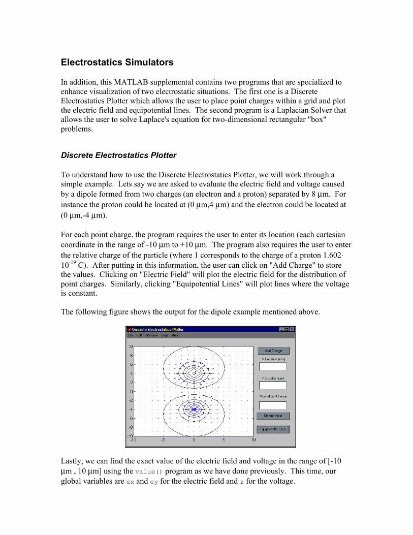
To understand how to use the Discrete Electrostatics Plotter, we will work through asimple example. Lets say we are asked to evaluate the electric field and voltage causedby a dipole formed from two charges (an electron and a proton) separated by 8 µm. Forinstance the proton could be located at (0 µm,4 µm) and the electron could be located at(0 µm,-4 µm).

For each point charge, the program requires the user to enter its location (each cartesiancoordinate in the range of -10 µm to +10 µm. The program also requires the user to enterthe relative charge of the particle (where 1 corresponds to the charge of a proton 1.602⋅10-19 C). After putting in this information, the user can click on "Add Charge" to storethe values. Clicking on "Electric Field" will plot the electric field for the distribution ofpoint charges. Similarly, clicking "Equipotential Lines" will plot lines where the voltageis constant.

The following figure shows the output for the dipole example mentioned above.

Lastly, we can find the exact value of the electric field and voltage in the range of [-10µm , 10 µm] using the value() program as we have done previously. This time, ourglobal variables are ex and ey for the electric field and z for the voltage.

For instance, the following sequence of commands will tell us the electric field andvoltage at the location (2 µm, 2 µm).

Ex = value('ex',-10,10,-10,10,2,2)Ey = value('ey',-10,10,-10,10,2,2)V = value('z',-10,10,-10,10,2,2)

Laplacian Solver

The Laplacian Solver allows the user to set up boundary values for a two-dimensionalrectangle and then evaluate the voltage within this region. The boundaries that the regionhas include the four sides (top, bottom, left, and right) as well as any number of "potentialnodes" the user would like to add.

For example, if we would like to solve a problem where the top and bottom edges have avalue of 1 Volt along their lengths, the left and right edges are grounded (0 Volts), andthere are two potential nodes within the region (say of magnitude 0.8 Volts and 1.2 Voltsshown in figure below), then we would use the Laplacian Solver as in the followingfigure.

Notice that after clicking "Plot Voltage," the program generates both a contour plot and athree-dimension surface plot. To animate a rotation of the surface plot, typeanimlaplace after running the simulator. For a sample animation type show('rotat').For this program, the global variable to be used with value() to evaluate the voltage is v.

Sample Problems

All of the following exercises should be completed with MATLAB and where appropriateverified through hand analysis.

For problems 1 → 4 assume v(x,y) = x2y

1) Given a point charge of Q = 1 µC, use the Discrete Electrostatics Plotter to plot theelectric field around this point.

2) Compare E(2 µm, 2 µm) found with the Discrete Electrostatics Plotter for the pointcharge in the previous problem to that found using the Gradient Plotter (by E = -∇V)to the actual value.

3) What could explain the differences in the previous problem? Modify the source codeto yield a more accurate result. What are the costs of such a change?

4) Find the voltage at (8 µm, 8 µm) caused by a quadruple of four protons located at (0,1 µm), (0, -1 µm), (1 µm,0), and (-1 µm,0).

5) Plot the equipotential lines for a random network of 10 point charges.6) Write a MATLAB script to perform the same tasks as the Discrete Electrostatics

Plotter except to output the results in three dimensions. Consider using quiver3() todraw the field lines and slice() to illustrate the voltage distribution.

7) Repeat the previous problem except for the Laplacian Solver.8) If all four sides of a box are at a potential of 1 V, plot the voltage within the box using

the Laplacian Solver.9) What is the voltage at (2,2) for the previous problem?10) Compare the answer found in problem 9 with the actual value (found with separation

of variables).11) Repeat problem 8 with a voltage node of -2 V at the center of the box.12) Repeat problem 9 with a voltage node of -2 V at the center of the box.13) Calculate the computation time for the successive over-relaxation algorithm for a box

with all four sides grounded (0 V) and 2 point charges of 1 V each at (5,15) and(25,15) by modifying the source code to include the tic() and toc() commands.Also determine the number of floating point operations required for this algorithmusing the flops() command. How would you rate this method of numericalanalysis?

14) Plot the voltage for a two dimensional rectangle if the boundary conditions for eachside are such that the voltage from one end to another goes through one cycle of acosine wave.

15) Find the resistance per unit length, R, of a block of conducting material with width W,thickness t, length L, contact thickness T, and conductivity σ. Plot R versus T/W forthe cases W/L = 2/3, 1, and 1.5. To solve this problem, you will have to modify theLaplacian Solver to handle a special boundary condition. In addition, you will haveto write a small code to calculate a partial derivative on a mesh. (Hint: Think of how

you would solve the problem by hand, and then just apply it to MATLAB making useof the codes that are already written for you.)

Source Codes(The initialization overhead has been omitted to conserve space.)

Animlaplace.m

function animlaplace%% animlaplace.m%% This program will take the voltage distribution output from laplace.m% and create an animation of a rotation of the surface plot.%

global vfigure

% allocate memoryn = 25; % number of framesM = moviein(n);i = 1;

colormap('gray')h = surfl(linspace(0,1.5,30),linspace(0,1,20),v);shading('interp')axis('off');

for angle=linspace(0,9*pi,25) rotate(h,[0 0],angle) axis([0 1.5 0 1 min(min(v)) max(max(v))]) % pause was included so that I could copy images into Paint Shop Pro %pause; M(:,i) = getframe; i = i+1;end

closeclosesave('rotat','M')clearshow('rotat')

curl.m

function curl(action)%% curl.m%% This program will allow the user to play with curl operations on% vector fields.

%

% declare global variablesglobal formula1global formula2global mesh1global mesh2global mesh3global mesh4global pointxglobal pointyglobal time1global time2global c

if nargin < 1action = 'initialize';

end

if strcmp(action,'initialize')

[ initialization routine ]

end

if strcmp(action,'plot_vector')

% read in parameters x_formula = get(formula1,'String'); y_formula = get(formula2,'String'); xmin = str2num(get(mesh1,'String')); xmax = str2num(get(mesh2,'String')); ymin = str2num(get(mesh3,'String')); ymax = str2num(get(mesh4,'String'));

% set up grid with 20 steps [x y] = meshgrid(linspace(xmin,xmax,20),linspace(ymin,ymax,20));

% plot vector field v = (dx,dy) dx = eval(x_formula); dy = eval(y_formula); quiver(x,y,dx,dy,0.5,'r'); axis([xmin xmax ymin ymax]);

end

if strcmp(action,'plot_drop')

% read in parameters x_formula = get(formula1,'String'); y_formula = get(formula2,'String'); xmin = str2num(get(mesh1,'String')); xmax = str2num(get(mesh2,'String')); ymin = str2num(get(mesh3,'String')); ymax = str2num(get(mesh4,'String')); t1 = str2num(get(time1,'String')); t2 = str2num(get(time2,'String'));

px = str2num(get(pointx,'String')); py = str2num(get(pointy,'String')); l = 1/4*min(xmax-xmin,ymax-ymin); px2 = px+l; py2 = py+l;



% set up function file fid = fopen('vector.m','w'); fprintf(fid,'function xdot = vector(t,f)\n'); fprintf(fid,'x=f(1);\ny=f(2);\n'); fprintf(fid,'xdot = [%s;%s];',x_formula,y_formula); fclose(fid); % xdot = [x_formula;y_formula] % corresponds to system of ordinary differential equations % x' = x_formula, y' = y_formula

% solve differential equation for flowline of vector field [ta,p1] = ode113('vector',[t1 t2],[px;py]); [tb,p2] = ode113('vector',[t1 t2],[px2;py2]); % fix so ta and tb same size if size(tb,1)>size(ta,1) for i = 1:(size(tb,1)-size(ta,1)) p1(size(ta,1)+i,1)=p1(size(ta,1),1); p1(size(ta,1)+i,2)=p1(size(ta,1),2); end elseif size(tb,1)<size(ta,1) for i = 1:(size(ta,1)-size(tb,1)) p2(size(tb,1)+i,1)=p2(size(tb,1),1); p2(size(tb,1)+i,2)=p2(size(tb,1),2); end end

for i = 1:size(p1,1) m = (p2(i,2)-p1(i,2))/(p2(i,1)-p1(i,1)); b = p1(i,2)-m*p1(i,1); pcx = l/4*(1/sqrt(1+m^2))+p1(i,1); pcy = m*(pcx-p1(i,1))+p1(i,2); p2(i,1) = l*(1/sqrt(1+m^2))+p1(i,1); p2(i,2) = m*(p2(i,1)-p1(i,1))+p1(i,2); m2 = -1/m; b2 = pcy-m2*pcx; p3(i,1) = l/4*(1/sqrt(1+m2^2))+pcx; p3(i,2) = m2*(p3(i,1)-pcx)+pcy; p4(i,1) = -l/4*(1/sqrt(1+m2^2))+pcx; p4(i,2) = m2*(p4(i,1)-pcx)+pcy; end

% adjust ordering of points

for i = 1:size(p1,1) temp1 = p2(i,1); temp2 = p2(i,2); p2(i,1) = p3(i,1); p2(i,2) = p3(i,2); p3(i,1) = temp1; p3(i,2) = temp2; end

% plot flowline hold on patch([p1(1,1),p2(1,1),p3(1,1),p4(1,1)],... [p1(1,2),p2(1,2),p3(1,2),p4(1,2)],'b'); plot(p1(1:size(p1,1),1),p1(1:size(p1,1),2),'k'); plot(p1(size(p1,1),1),p1(size(p1,1),2),'kd');

H = line([p1(size(p1,1),1) p2(size(p1,1),1)],[p1(size(p1,1),2) ... p2(size(p1,1),2)]); set(H,'color','k'); set(H,'LineStyle',':'); H = line([p2(size(p1,1),1) p3(size(p1,1),1)],[p2(size(p1,1),2) ... p3(size(p1,1),2)]); set(H,'color','k'); set(H,'LineStyle',':'); H = line([p3(size(p1,1),1) p4(size(p1,1),1)],[p3(size(p1,1),2) ... p4(size(p1,1),2)]); set(H,'color','k'); set(H,'LineStyle',':'); H = line([p4(size(p1,1),1) p1(size(p1,1),1)],[p4(size(p1,1),2) ... p1(size(p1,1),2)]); set(H,'color','k'); set(H,'LineStyle',':'); patch([p1(size(p1,1),1),p2(size(p1,1),1),p3(size(p1,1),1), ... p4(size(p1,1),1)],[p1(size(p1,1),2),p2(size(p1,1),2), ... p3(size(p1,1),2),p4(size(p1,1),2)],'b');

axis([xmin xmax ymin ymax]); hold off

end % plot_drop routine

if strcmp(action,'plot_curl')

% read in parameters clear x_formula clear y_formula x_formula = get(formula1,'String'); y_formula = get(formula2,'String'); xmin = str2num(get(mesh1,'String')); xmax = str2num(get(mesh2,'String')); ymin = str2num(get(mesh3,'String')); ymax = str2num(get(mesh4,'String'));


% vector field v = (dx,dy)

dx = eval(x_formula); dy = eval(y_formula);

% approximate derivatives using differences % dbdx represents d/dx(y_formula) % dady represents d/dy(x_formula) for i=1:size(dy,1) % = size(dy,1) dbdx(i,:) = diff(dy(i,:))./diff(x(i,:)); end for i=1:size(dx,2) % = size(dy,1) dady(:,i) = diff(dx(:,i))./diff(y(:,i)); end dbdx(:,size(dbdx,2)+1)=dbdx(:,size(dbdx,2)); dady(size(dady,1)+1,:)=dady(size(dady,1),:); c = dbdx-dady; meshc(x,y,c); brighten(-1); hold on surfl(x,y,c); shading('interp'); colormap('gray') hold off

end % plot_curl routine

divergence.m

function divergence(action)%% divergence.m%% This program will allow the user to play with divergence operations% on vector fields.%

% declare global variablesglobal formula1global formula2global mesh1global mesh2global mesh3global mesh4global point1global point2global point3global point4global time1global time2global d


end


[ initialization routine ]end


% read in parameters x_formula = get(formula1,'String'); y_formula = get(formula2,'String'); xmin = str2num(get(mesh1,'String')); xmax = str2num(get(mesh2,'String')); ymin = str2num(get(mesh3,'String')); ymax = str2num(get(mesh4,'String'));



end % plot_vector routine

if strcmp(action,'plot_drop')

% read in parameters x_formula = get(formula1,'String'); y_formula = get(formula2,'String'); xmin = str2num(get(mesh1,'String')); xmax = str2num(get(mesh2,'String')); ymin = str2num(get(mesh3,'String')); ymax = str2num(get(mesh4,'String')); t1 = str2num(get(time1,'String')); t2 = str2num(get(time2,'String')); t = str2num(get(point1,'String')); x1 = t(1); y1 = t(2); t = str2num(get(point2,'String')); x2 = t(1); y2 = t(2); t = str2num(get(point3,'String')); x3 = t(1); y3 = t(2); t = str2num(get(point4,'String')); x4 = t(1); y4 = t(2);


% plot vector field v = (dx,dy) dx = eval(x_formula); dy = eval(y_formula); quiver(x,y,dx,dy,0.5,'r');

axis([xmin xmax ymin ymax]);

% set up function file fid = fopen('vector.m','w'); fprintf(fid,'function xdot = vector(t,f)\n'); fprintf(fid,'x=f(1);\ny=f(2);\n'); fprintf(fid,'xdot = [%s;%s];',x_formula,y_formula); fclose(fid); % xdot = [x_formula;y_formula] % corresponds to system of ordinary differential equations % x' = x_formula, y' = y_formula

% solve differential equation for flowline of vector field [ta,p1] = ode113('vector',[t1 t2],[x1;y1]); [tb,p2] = ode113('vector',[t1 t2],[x2;y2]); [tc,p3] = ode113('vector',[t1 t2],[x3;y3]); [td,p4] = ode113('vector',[t1 t2],[x4;y4]);

% plot flowlines hold on fill([p1(1,1),p2(1,1),p3(1,1),p4(1,1)],...

[p1(1,2),p2(1,2),p3(1,2),p4(1,2)],'b'); plot(p1(1:size(ta,1),1),p1(1:size(ta,1),2),'k', ...

p2(1:size(tb,1),1),p2(1:size(tb,1),2),'k', ... p3(1:size(tc,1),1),p3(1:size(tc,1),2),'k', ...

p4(1:size(td,1),1),p4(1:size(td,1),2),'k'); plot(p1(size(ta,1),1),p1(size(ta,1),2),'kd',...

p2(size(tb,1),1),p2(size(tb,1),2),'kd', ... p3(size(tc,1),1),p3(size(tc,1),2),'kd',...

p4(size(td,1),1),p4(size(td,1),2),'kd'); H = line([p1(size(ta,1),1) p2(size(tb,1),1)],...

[p1(size(ta,1),2) p2(size(tb,1),2)]); set(H,'color','k'); set(H,'LineStyle',':'); H = line([p2(size(tb,1),1) p3(size(tc,1),1)],...

[p2(size(tb,1),2) p3(size(tc,1),2)]); set(H,'color','k'); set(H,'LineStyle',':'); H = line([p3(size(tc,1),1) p4(size(td,1),1)],...

[p3(size(tc,1),2) p4(size(td,1),2)]); set(H,'color','k'); set(H,'LineStyle',':'); H = line([p4(size(td,1),1) p1(size(ta,1),1)],...

[p4(size(td,1),2) p1(size(ta,1),2)]); set(H,'color','k'); set(H,'LineStyle',':'); axis([xmin xmax ymin ymax]); hold off

end % plot_drop routine

if strcmp(action,'plot_div')

% read in parameters x_formula = get(formula1,'String'); y_formula = get(formula2,'String'); xmin = str2num(get(mesh1,'String'));

xmax = str2num(get(mesh2,'String')); ymin = str2num(get(mesh3,'String')); ymax = str2num(get(mesh4,'String'));


% plot vector field v = (dx,dy) dx = eval(x_formula); dy = eval(y_formula);

% approximate derivatives using differences % dadx represents d/dx(x_formula) % dbdy represents d/dy(y_formula) for i=1:size(dx,1) % = size(dy,1) dadx(i,:) = diff(dx(i,:))./diff(x(i,:)); end for i=1:size(dx,2) % = size(dy,1) dbdy(:,i) = diff(dy(:,i))./diff(y(:,i)); end dadx(:,size(dadx,2)+1)=dadx(:,size(dadx,2)); dbdy(size(dbdy,1)+1,:)=dbdy(size(dbdy,1),:); d = dadx+dbdy; meshc(x,y,d); brighten(-1); hold on surfl(x,y,d); shading('interp'); colormap('gray') hold off

end % plot_div routine

elect.m

function elect(action)%% elect.m%% This program will allow the user to play with discrete electrostatic% fields and equipotential lines%

% declare global variablesglobal xglobal yglobal qglobal xlocglobal ylocglobal qlocglobal numglobal zglobal exglobal ey


end


[ intialization routine ]

end

if strcmp(action,'add')

xloc(num) = str2num(get(x,'String')); yloc(num) = str2num(get(y,'String')); qloc(num) = str2num(get(q,'String')); if xloc(num)>10 | xloc(num)<-10 error('Location must be in range of [-10,10]'); close elseif yloc(num)>10 | yloc(num)<-10 error('Location must be in range of [-10,10]'); close elseif qloc(num)==0 error('Zero Charge Entered!'); close else num = num+1; set(x,'String',''); set(y,'String','');

set(q,'String','');% clear axisplot(0,0,'w')% plot points with labelsfor i = 1:(num-1) hold on

plot(xloc(i),yloc(i),'ko'); hold off

text(xloc(i)+0.2,yloc(i)+0.2,num2str(qloc(i))); end axis([-10 10 -10 10]); end

end

if strcmp(action,'plot_field')|strcmp(action,'plot_volt')

e0 = 8.854e-12; q0 = 1.6e-19;

v = 'q0/(4*pi*e0)*('; for i = 1:(num-1) if(i==1) term = sprintf('%f.*1e6./sqrt((xg-%f).^2+ ...

(yg-%f).^2)',qloc(i),xloc(i),yloc(i)); else term = sprintf('+%f.*1e6./sqrt((xg-%f).^2+ ...

(yg-%f).^2)',qloc(i),xloc(i),yloc(i)); end

v = strcat(v,term); end v = strcat(v,')');

[xg yg] = meshgrid(linspace(-10,10,20),linspace(-10,10,20)); z = eval(v); for i = 1:size(z,1) for j = 1:size(z,2) if isinf(z(i,j)) temp = num2str(z(i,j)); if size(temp,2)==3 % Inf Case z(i,j) = 1.2*(abs(z(i+1,j))+ ...

abs(z(i-1,j))+abs(z(i,j+1))+abs(z(i,j-1)))/4; elseif size(temp,2)==4 % -Inf Case z(i,j) = -1.2*(abs(z(i+1,j))+...

abs(z(i-1,j))+abs(z(i,j+1))+abs(z(i,j-1)))/4; end end z(i,j) = -1*z(i,j); end end

[ex,ey] = gradient(z); hold on quiver(xg,yg,ex,ey) hold off

for i = 1:size(z,1) for j = 1:size(z,2) z(i,j) = -1*z(i,j); end end

if strcmp(action,'plot_volt') hold on contour(xg,yg,z,10,'k') hold off end

end

fluxint.m

function fluxint(action)%% fluxint.m%% This program will allow the user to play with flux integrals on% vector fields.%

% declare global variablesglobal formulax

global formulayglobal formulazglobal formulasglobal resultglobal x1global y1global z1global x2global y2global z2


end



end


fx = get(formulax,'String'); fy = get(formulay,'String'); fz = get(formulaz,'String'); xmin = str2num(get(x1,'String')); xmax = str2num(get(x2,'String')); ymin = str2num(get(y1,'String')); ymax = str2num(get(y2,'String')); zmin = str2num(get(z1,'String')); zmax = str2num(get(z2,'String'));

% set up grid with 10 steps [x y z] = meshgrid(linspace(xmin,xmax,10), ...

linspace(ymin,ymax,10),linspace(zmin,zmax,10));

% plot vector field dx = eval(fx); dy = eval(fy); dz = eval(fz); quiver3(x,y,z,dx,dy,dz,0.5,'r'); axis([xmin xmax ymin ymax zmin zmax]);

end

if strcmp(action,'plot_surface')

fx = get(formulax,'String'); fy = get(formulay,'String'); fz = get(formulaz,'String'); zs = get(formulas,'String') xmin = str2num(get(x1,'String')); xmax = str2num(get(x2,'String')); ymin = str2num(get(y1,'String')); ymax = str2num(get(y2,'String')); zmin = str2num(get(z1,'String'));

zmax = str2num(get(z2,'String'));


% plot vector field dzs = eval(zs); zmax = max(max(dzs,[],1)); zmin = min(min(dzs,[],1)); [x y z] = meshgrid(linspace(xmin,xmax,10), ...

linspace(ymin,ymax,10),linspace(zmin,zmax,10)); dx = eval(fx); dy = eval(fy); dz = eval(fz); quiver3(x,y,z,dx,dy,dz,0.5,'r');

% plot surface hold on [x y] = meshgrid(linspace(xmin,xmax,10),linspace(ymin,ymax,10)); surf(x,y,dzs) SHADING interp colormap(gray) hold off axis([xmin xmax ymin ymax zmin zmax]);

end

if strcmp(action,'calc_flux')

fx = get(formulax,'String'); fy = get(formulay,'String'); fz = get(formulaz,'String'); zs = get(formulas,'String'); xmin = str2num(get(x1,'String')); xmax = str2num(get(x2,'String')); ymin = str2num(get(y1,'String')); ymax = str2num(get(y2,'String')); zmin = str2num(get(z1,'String')); zmax = str2num(get(z2,'String'));

[x y] = meshgrid(linspace(xmin,xmax,10),linspace(ymin,ymax,10)); dzs = eval(zs); zmax = max(max(dzs,[],1)); zmin = min(min(dzs,[],1)); [x y z] = meshgrid(linspace(xmin,xmax,10),...

linspace(ymin,ymax,10),linspace(zmin,zmax,10)); dx = eval(fx); dy = eval(fy); dz = eval(fz); [x y] = meshgrid(linspace(xmin,xmax,10),linspace(ymin,ymax,10)); [nx ny nz] = surfnorm(dzs);

hold on quiver3(x,y,dzs,nx,ny,nz); hold off

% set up function file

fid = fopen('vector3.m','w'); fprintf(fid,'function f = vector3(x,y)\n');

fprintf(fid,'x1 = %f;\n',xmin); fprintf(fid,'x2 = %f;\n',xmax); fprintf(fid,'y1 = %f;\n',ymin); fprintf(fid,'y2 = %f;\n',ymax); fprintf(fid,'[xa ya] = meshgrid(linspace(x1,x2,10), ...

linspace(y1,y2,10));\n'); fprintf(fid,'z = ''%s'';\n',zs); fprintf(fid,'z = strrep(z,''y'',''ya'');\n'); fprintf(fid,'z = strrep(z,''x'',''xa'');\n'); fprintf(fid,'z = eval(z);\n'); fprintf(fid,'for i=1:size(z,1)\n'); fprintf(fid,'dfdx(i,:) = diff(z(i,:))./diff(xa(i,:));\n'); fprintf(fid,'dfdy(:,i) = diff(z(:,i))./diff(ya(:,i));\n'); fprintf(fid,'end\n'); fprintf(fid,'nx = -dfdx;\n'); fprintf(fid,'ny = -dfdy;\n'); fprintf(fid,'nz = ones(size(dfdx));\n');

fprintf(fid,'if size(x,2)==size(y,2)\n'); fprintf(fid,'l = size(x,2);\n'); fprintf(fid,'elseif size(x,2)==1\n'); fprintf(fid,'x = x.*ones(size(y));\n'); fprintf(fid,'l = size(x,2);\n'); fprintf(fid,'elseif size(y,2)==1\n'); fprintf(fid,'y = y.*ones(size(x));\n'); fprintf(fid,'l = size(x,2);\n'); fprintf(fid,'end\n'); fprintf(fid,'z = %s;\n',zs); fprintf(fid,'for i = 1:l\n'); fx = strrep(fx,'x','x(i)'); fx = strrep(fx,'y','y(i)'); fx = strrep(fx,'z','z(i)'); fy = strrep(fy,'x','x(i)'); fy = strrep(fy,'y','y(i)'); fy = strrep(fy,'z','z(i)'); fz = strrep(fz,'x','x(i)'); fz = strrep(fz,'y','y(i)'); fz = strrep(fz,'z','z(i)'); fprintf(fid,'v(i,:) = [%s %s %s];\n',fx,fy,fz); fprintf(fid,'end\n'); fprintf(fid,'for i = 1:l\n'); fprintf(fid,'xindex(i)=round((x(i)-x1)/(x2-x1)*(size(xa,2)));\n'); fprintf(fid,'yindex(i)=round((y(i)-y1)/(y2-y1)*(size(ya,2)));\n'); fprintf(fid,'end\n'); fprintf(fid,'for j=1:size(xindex,2)\n'); fprintf(fid,'if xindex(j)<=0,xindex(j)=1;,end\n'); fprintf(fid,'if xindex(j)>=size(xa,2), ...

xindex(j)=size(xa,2)-1;,end\n'); fprintf(fid,'end\n'); fprintf(fid,'for j=1:size(yindex,2)\n'); fprintf(fid,'if yindex(j)<=0,yindex(j)=1;,end\n'); fprintf(fid,'if yindex(j)>=size(ya,2), ...

yindex(j)=size(ya,2)-1;,end\n'); fprintf(fid,'end\n');

fprintf(fid,'for i = 1:l\n'); fprintf(fid,'n(i,:) = [nx(xindex(i),yindex(i)) ...

ny(xindex(i),yindex(i)) nz(xindex(i),yindex(i)) ];\n'); fprintf(fid,'end\n'); fprintf(fid,'for i=1:l\n'); fprintf(fid,'f(:,i) = dot(v(i,:),n(i,:));\n'); fprintf(fid,'end\n'); fclose(fid);

answer = dblquad('vector3',xmin,xmax,ymin,ymax); set(result,'String',num2str(answer));

end

grad.m

function grad(action)%% grad.m%% This program will allow the user to play with gradient operations on% vector fields.%

% declare global variablesglobal formulaglobal x1global y1global x2global y2global dxglobal dy


end



end

if strcmp(action,'plot_contour')

f = get(formula,'String'); xmin = str2num(get(x1,'String')); xmax = str2num(get(x2,'String')); ymin = str2num(get(y1,'String')); ymax = str2num(get(y2,'String'));


% plot contours

z = eval(f); c = contour(x,y,z); clabel(c);

end

if strcmp(action,'plot_gradient')

hold on f = get(formula,'String'); xmin = str2num(get(x1,'String')); xmax = str2num(get(x2,'String')); ymin = str2num(get(y1,'String')); ymax = str2num(get(y2,'String'));


% plot gradient z = eval(f); % approximate derivatives using differences % dx represents dz/dx % dy represents dz/dy dx = zeros(size(z,1)-1,size(z,2)-1); dy = zeros(size(z,1)-1,size(z,2)-1); for i=1:size(z,1) dx(i,:) = diff(z(i,:))./diff(x(i,:)); end for i=1:size(z,2) dy(:,i) = diff(z(:,i))./diff(y(:,i)); end dx(:,size(dx,2)+1)=dx(:,size(dx,2)); dy(size(dy,1)+1,:)=dy(size(dy,1),:);

quiver(x,y,dx,dy); hold off

end

laplace.m

function laplace(action)%% laplace.m%% This program will allow the user to play with solutions to Laplace's% equation for rectangular boundary conditions.%% Parts of this code were developed by Jason Papadopoulos.

% declare global variablesglobal xglobal yglobal valglobal top

global bottomglobal leftglobal rightglobal numglobal valueglobal vtopglobal vbottomglobal vleftglobal vrightglobal plot1global plot2global v


end



% initialize plot axes(plot2); axis('off'); axes(plot1); axis([-1 32 -1 22]) %xlabel('x') %ylabel('y') h = line([1 1 30 30 1],[1 20 20 1 1]); set(h,'Color','k'); num = 1;

end

if strcmp(action,'add_point')

val(num) = str2num(get(value,'String')); [x(num) y(num)] = ginput(1); if x(num)>30 | x(num)<1 error('X location must be in range of [1,30]'); close elseif y(num)>20 | y(num)<1 error('Y location must be in range of [1,20]'); close elseif isempty(val(num)) error('Must first enter voltage'); close else num = num+1; set(value,'String',''); % clear axis axes(plot1); plot(0,0,'w') axis([-2 32 -2 22])

h = line([1 1 30 30 1],[1 20 20 1 1]); set(h,'Color','k'); % plot points

for i = 1:(num-1) hold on

plot(x(i),y(i),'ro'); hold off

end end

end

if strcmp(action,'plot_voltage')

top = str2num(get(vtop,'String')); bottom = str2num(get(vbottom,'String')); left = str2num(get(vleft,'String')); right = str2num(get(vright,'String'));

% set up grid for "successive over relaxation" algorithm % rows = 20; % cols = 30;

v = zeros(20,30); for i = 1:(num-1) v(round(y(i)),round(x(i))) = val(i); end v(:,1) = left.*ones(20,1); v(:,30) = right.*ones(20,1); v(1,:) = top.*ones(1,30); v(20,:) = bottom.*ones(1,30);

overrelax = 1; for i = 1:20 for j = 2:19 for k = 2:29 temp = 0.25.*(v(j-1,k)+v(j+1,k)+v(j,k-1)+v(j,k+1)); v(j,k) = v(j,k) + overrelax*(temp-v(j,k)); for l = 1:(num-1) if j==round(y(l)) & k==round(x(l)) v(j,k) = val(l); end end end end end

axes(plot2); colormap('gray') surfl(linspace(0,1.5,30),linspace(0,1,20),v); shading('interp') axis('off');

axes(plot1); plot(0,0,'w'); axis([-2 32 -2 22]) h = line([1 1 30 30 1],[1 20 20 1 1]); set(h,'Color','k'); % plot points for i = 1:(num-1)

hold on plot(x(i),y(i),'ro');

hold off end hold on contour(v,15,'k'); hold off

end

lineints.m

function lineints(action)%% lineints.m%% This program will allow the user to play with line integrals on% scalar fields.%

% declare global variablesglobal formulaglobal resultglobal curveglobal statusglobal x1global y1global x2global y2global time1global time2global cxglobal cyglobal pxglobal py


end



end

if strcmp(action,'plot_contour')


% set up grid with 20 steps

[x y] = meshgrid(linspace(xmin,xmax,20),linspace(ymin,ymax,20));

% plot contours z = eval(f); c = contour(x,y,z,10); clabel(c); axis([xmin xmax ymin ymax]);

end

if strcmp(action,'plot_line')


[x y] = meshgrid(linspace(xmin,xmax,20),linspace(ymin,ymax,20)); z = eval(f);

val = get(curve,'Value'); val2 = get(status,'Value'); if val == 2 % Line Segments if val2 == 0 % Mouse Input [px py] = ginput(2); else % Keyboard Input disp('Enter Locations (X1,Y1) to (X2,Y2) ...'); disp(' '); px(1) = input('X1 = '); py(1) = input('Y1 = '); px(2) = input('X2 = '); py(2) = input('Y2 = '); end c = contour(x,y,z,10); clabel(c); axis([xmin xmax ymin ymax]); hold on l = line(px,py); set(l,'Color','k'); plot(px(2),py(2),'kd'); hold off else % Parametric Curve cfx = get(cx,'String'); cfy = get(cy,'String'); t1 = str2num(get(time1,'String')); t2 = str2num(get(time2,'String')); t = t1:(t2-t1)/500:t2-(t2-t1)/500; c = contour(x,y,z,10); clabel(c); axis([xmin xmax ymin ymax]); hold on xpt = eval(cfx); ypt = eval(cfy); plot(xpt,ypt,'k'); plot(xpt(size(xpt,2)),ypt(size(ypt,2)),'kd'); axis([xmin xmax ymin ymax]);

hold off end

end

if strcmp(action,'calc_line')

f = get(formula,'String');

val = get(curve,'Value'); if val == 2 % Line Segment % Split Line into 501 points (500 sections) xval = px(1):(px(2)-px(1))/501:px(2)-(px(2)-px(1))/501; yval = py(1):(py(2)-py(1))/501:py(2)-(py(2)-py(1))/501; if px(1) == px(2) xval = px(1).*ones([1 501]); end if py(1) == py(2) yval = py(1).*ones([1 501]); end for i=1:500 dx(i) = xval(i+1)-xval(i); dy(i) = yval(i+1)-yval(i); x = xval(i); y = yval(i); Fn(i) = eval(f); s1(i) = Fn(i)*dx(i); s2(i) = Fn(i)*dy(i); end ans1 = sum(s1); ans2 = sum(s2); else % Parametric Curve cfx = get(cx,'String'); cfy = get(cy,'String'); t1 = str2num(get(time1,'String')); t2 = str2num(get(time2,'String'));

fstr = strrep(f,'x',strcat('(',cfx,')')); fstr = strrep(fstr,'y',strcat('(',cfy,')')); fstr1 = strcat('(',fstr,')','.*','a'); fstr2 = strcat('(',fstr,')','.*','b');

% set up function file fid = fopen('vector1.m','w');

fprintf(fid,'function f = vector1(tt)\n'); fprintf(fid,'t1 = %f;\n',t1); fprintf(fid,'t2 = %f;\n',t2); fprintf(fid,'t = t1:(t2-t1)/700:t2;\n'); fprintf(fid,'xpt = %s;\n',cfx); fprintf(fid,'ypt = %s;\n',cfy); fprintf(fid,'dfxdt = diff(xpt)./diff(t);\n'); fprintf(fid,'dfydt = diff(ypt)./diff(t);\n'); fprintf(fid,'index=round((tt-t1)/(t2-t1)*(size(t,2)));\n'); fprintf(fid,'for j=1:size(index,2)\n'); fprintf(fid,'if index(j)<=0,index(j)=1;,end\n'); fprintf(fid,'if index(j)>=size(t,2), ...

index(j)=size(t,2)-1;,end\n');

fprintf(fid,'end\n'); fprintf(fid,'t=tt;\n'); fprintf(fid,'a=dfxdt(index);\nb=dfydt(index);\n'); fprintf(fid,'f=%s;\n',fstr1);

fclose(fid); ans1 = quad8('vector1',t1,t2);

fid = fopen('vector2.m','w');fprintf(fid,'function f = vector2(tt)\n');

fprintf(fid,'t1 = %f;\n',t1); fprintf(fid,'t2 = %f;\n',t2); fprintf(fid,'t = t1:(t2-t1)/700:t2;\n'); fprintf(fid,'xpt = %s;\n',cfx); fprintf(fid,'ypt = %s;\n',cfy); fprintf(fid,'dfxdt = diff(xpt)./diff(t);\n'); fprintf(fid,'dfydt = diff(ypt)./diff(t);\n'); fprintf(fid,'index=round((tt-t1)/(t2-t1)*(size(t,2)));\n'); fprintf(fid,'for j=1:size(index,2)\n'); fprintf(fid,'if index(j)<=0,index(j)=1;,end\n'); fprintf(fid,'if index(j)>=size(t,2), ...

index(j)=size(t,2)-1;,end\n'); fprintf(fid,'end\n'); fprintf(fid,'t=tt;\n'); fprintf(fid,'a=dfxdt(index);\nb=dfydt(index);\n'); fprintf(fid,'f=%s;\n',fstr2);

fclose(fid); ans2 = quad8('vector2',t1,t2);

end answer = strcat('(',num2str(ans1),',',num2str(ans2),')'); set(result,'String',answer);

end

lineintv.m

function lineintv(action)%% lineintv.m%% This program will allow the user to play with line integrals on% vector fields.%

% declare global variablesglobal formulaxglobal formulayglobal resultglobal curveglobal statusglobal x1global y1global x2global y2global time1

global time2global cxglobal cyglobal pxglobal py


end



end


fx = get(formulax,'String'); fy = get(formulay,'String'); xmin = str2num(get(x1,'String')); xmax = str2num(get(x2,'String')); ymin = str2num(get(y1,'String')); ymax = str2num(get(y2,'String'));


% plot vector field dx = eval(fx); dy = eval(fy); quiver(x,y,dx,dy,0.5,'r'); axis([xmin xmax ymin ymax]);

end

if strcmp(action,'plot_line')

fx = get(formulax,'String'); fy = get(formulay,'String'); xmin = str2num(get(x1,'String')); xmax = str2num(get(x2,'String')); ymin = str2num(get(y1,'String')); ymax = str2num(get(y2,'String'));

[x y] = meshgrid(linspace(xmin,xmax,20),linspace(ymin,ymax,20)); dx = eval(fx); dy = eval(fy);

val = get(curve,'Value'); val2 = get(status,'Value'); if val == 2 % Line Segments if val2 == 0 % Mouse Input [px py] = ginput(2); else % Keyboard Input disp('Enter Locations (X1,Y1) to (X2,Y2) ...'); disp(' ');

px(1) = input('X1 = '); py(1) = input('Y1 = '); px(2) = input('X2 = '); py(2) = input('Y2 = '); end quiver(x,y,dx,dy,0.5,'r'); axis([xmin xmax ymin ymax]); hold on line(px,py); plot(px(2),py(2),'bd'); hold off else % Parametric Curve cfx = get(cx,'String'); cfy = get(cy,'String'); t1 = str2num(get(time1,'String')); t2 = str2num(get(time2,'String')); t = t1:(t2-t1)/500:t2-(t2-t1)/500; quiver(x,y,dx,dy,0.5,'r'); axis([xmin xmax ymin ymax]); hold on xpt = eval(cfx); ypt = eval(cfy); plot(xpt,ypt,'b'); plot(xpt(size(xpt,2)),ypt(size(ypt,2)),'bd'); axis([xmin xmax ymin ymax]); hold off end

end

if strcmp(action,'calc_line')

fx = get(formulax,'String'); fy = get(formulay,'String');

val = get(curve,'Value'); if val == 2 % Line Segment % Split Line into 501 points (500 sections) xval = px(1):(px(2)-px(1))/501:px(2)-(px(2)-px(1))/501; yval = py(1):(py(2)-py(1))/501:py(2)-(py(2)-py(1))/501; if px(1) == px(2) xval = px(1).*ones([1 501]); end if py(1) == py(2) yval = py(1).*ones([1 501]); end for i=1:500 dr(i,1) = xval(i+1)-xval(i); dr(i,2) = yval(i+1)-yval(i); x = xval(i); y = yval(i); Fn(i,1) = eval(fx); Fn(i,2) = eval(fy); s(i) = dot(Fn(i),dr(i)); end answer = sum(s); else % Parametric Curve

cfx = get(cx,'String'); cfy = get(cy,'String'); t1 = str2num(get(time1,'String')); t2 = str2num(get(time2,'String'));

fstrx = strrep(fx,'x',strcat('(',cfx,')')); fstrx = strrep(fstrx,'y',strcat('(',cfy,')')); fstry = strrep(fy,'x',strcat('(',cfx,')')); fstry = strrep(fstry,'y',strcat('(',cfy,')')); fstr = strcat('(',fstrx,')','.*','a','+','(',fstry,')','.*','b');

% set up function file fid = fopen('vector.m','w');

fprintf(fid,'function f = vector(tt)\n'); fprintf(fid,'t1 = %f;\n',t1); fprintf(fid,'t2 = %f;\n',t2); fprintf(fid,'t = linspace(t1,t2,700);\n'); fprintf(fid,'xpt = %s;\n',cfx); fprintf(fid,'ypt = %s;\n',cfy); fprintf(fid,'dfxdt = diff(xpt)./diff(t);\n'); fprintf(fid,'dfydt = diff(ypt)./diff(t);\n'); fprintf(fid,'index=round((tt-t1)/(t2-t1)*(size(t,2)));\n'); fprintf(fid,'for j=1:size(index,2)\n'); fprintf(fid,'if index(j)<=0,index(j)=1;,end\n'); fprintf(fid,'if index(j)>=size(t,2), ...

index(j)=size(t,2)-1;,end\n'); fprintf(fid,'end\n'); fprintf(fid,'t=tt;\n'); fprintf(fid,'a=dfxdt(index);\nb=dfydt(index);\n'); fprintf(fid,'f=%s;\n',fstr);

fclose(fid);

answer = quad8('vector',t1,t2);

%Approximate Integral Using Riemann Sum %t1 = str2num(get(time1,'String')); %t2 = str2num(get(time2,'String')); %t = t1:(t2-t1)/501:t2-(t2-t1)/501; %dt = (t2-t1)/501; %xpt = eval(cfx); %ypt = eval(cfy); %dfxdt = diff(xpt)./diff(t); %dfydt = diff(ypt)./diff(t); %for i=1:500 % dr(i,1) = dt*dfxdt(i); % dr(i,2) = dt*dfydt(i); % x = xpt(i); % y = ypt(i); % Fn(i,1) = eval(fx); % Fn(i,2) = eval(fy); % s(i) = dot(Fn(i),dr(i)); %end %answer = sum(s); end set(result,'String',num2str(answer));

end

show.m

function show(name)%% show.m%% This file is used to load saved animations.%

load(name);if(name(1)=='r') colormap('gray') shading('interp')endmovie(M,1);

start.m

% start.m%% This program launches a menu to run other applications.%

Y = wavread('tada.wav');sound(Y);

K = menu('ENEE 380 MATLAB Programs', ... 'Gradient Plotter','Divergence Plotter','Curl Plotter', ... 'Scalar Line Integrator','Vector Line Integrator','Flux Integrator',... 'Discrete Electrostatics Plotter','Laplacian Solver');

switch Kcase 1, grad;case 2, divergence;case 3, curl;case 4, lineints;case 5, lineintv;case 6, fluxint;case 7, elect;case 8, laplace;end

value.m

function val = value(name,xmin,xmax,ymin,ymax,x,y)%% value(name,xmin,xmax,ymin,ymax,x,y)%% This file will, given a two dimension matrix, convert between meshvalues and% matrix indices to obtain an element.%% Parameters:%% name = a string with the name of global variable% xmin = minimum mesh x range% xmax = maximum mesh x range% ymin = minimum mesh y range% ymax = maximum mesh y range% x = x value to return% y = y value to return%

% Declare variable to be globaleval(sprintf('global %s',name));

% Evaluate indexif isempty(eval([name])) error('Variable doesn''t exist');elseif (xmin >= xmax) | (ymin >= ymax) | (x > xmax) | (x < xmin) | ... (y > ymax) | (y < ymin) error('Range error');else % name(rows,cols) = rows are y values; cols are x values xrange = linspace(xmin,xmax,eval(sprintf('size(%s,2)',name))); xstep = abs(xrange(2)-xrange(1)); xval = find( (xrange <= (x+xstep/2)) & (xrange > (x-xstep/2)) );

yrange = linspace(ymin,ymax,eval(sprintf('size(%s,1)',name))); ystep = abs(yrange(2)-yrange(1)); yval = find( (yrange <= (y+ystep/2)) & (yrange > (y-ystep/2)) );

val = eval(sprintf('%s(yval,xval)',name));end

EELECTROSTATICS WITHLECTROSTATICS WITH...

Documents

Transcript of EELECTROSTATICS WITHLECTROSTATICS WITH...