Eee598 Project New

STABILITY ANALYSIS OF A SAMPLE FOUR

MACHINE SYSTEM USING CLASSICAL MODEL

WITH THE HELP OF PSLF

A PROJECT REPORT

Submitted by

Members of Group 5

Fei Gao

Supriya Chathadi

Changxu Chen

Habibou Maiga

Submitted to

Dr. Vijay Vittal

In partial fulfillment for completion of the course

EEE598: POWER SYSTEM STABILITY

at

ARIZONA STATE UNIVERSITY, TEMPE

EEE598-Group 5

Arizona State University 2

Table of Contents

1. Introduction ............................................................................................................................. 3 2. Input Data Files ....................................................................................................................... 4

2.1 Power Flow Case File ............................................................................................................4

2.2 Transient Stability File ...........................................................................................................4 3. Transient Simulation Description and Results ........................................................................... 4

3.1 Relative Rotor Angles Plots .................................................................................................10

3.2 Absolute Rotor Angle Plots ................................................. Error! Bookmark not defined. 4. Shortcomings of Classical Model ............................................................................................. 12 5. Inference ................................................................................................................................ 12 6. References ............................................................................................................................. 13 Appendix 1 ................................................................................................................................... i Appendix 2 ................................................................................................................................. iii Appendix 3 .................................................................................................................................. v

APPENDICES

APPENDIX 1 PSLF Power Flow Mismatch

APPENDIX 2 PSLF Dynamic Data File

APPENDIX 3 One Line Diagram

EEE598-Group 5


1. Introduction

This report documents the results of the transient stability study performed for the project using

the PSLF software. The project assigned is to:

a. Prepare a dynamic data file for the given four machine, six bus system (shown in

Appendix 3) with the classical model from the detailed machine model which is given.

b. Simulate a 3-phase short circuit at bus 5 and determine the critical clearing time.

c. Plot the relative and absolute angles for all the machines and determine the stability of

the system; conclude which among the two is better to measure the loss in

synchronism.

A brief overview of the procedure is presented below in the form of a flowchart in Figure 1.

Detailed explanation and results follow.

Figure 1

Import „.raw‟ file

Solve Power Flow

Prepare the dynamic data file, „.dat‟ for four generators

with classical model

Read and Initiate the „.dat‟ file

Run pre-fault, faulted & post-fault simulations with reference bus

specified (relative rotor angle plot) and find critical clearing time (by

trial and error)

Run pre-fault, faulted & post-fault simulations with reference bus

zeroed (absolute rotor angle plot) and find critical clearing time (by

trial and error)

EEE598-Group 5


2. Input Data Files

2.1 Power Flow Case File

The raw file from [1] is imported into the PSLF software using the “Import PTI” option. This

creates the PSLF case file for the sample four machine system. The “solv” command is used to

solve the power flow. As the mismaches are almost negligible (Appendix 1 shows the results),

we conclude that the power flow converges.

2.2 Transient Stability File

The dynamic data given in [2] is for a detailed machine model. A simplified PSLF dynamic

data file which models all the four machines with the classical model was created and is shown

in appendix 2. Only the sub transient reactance ( xd'), and inertia constant (H) of the generators

are used. (The syntax for the classical generator model in the dynamic file was written from

page 809 of [3]). The “rdyd” command in PSLF is used to read the file and “init” is used to

initiate it.

3. Transient Simulation Description and Results

A stable power system is one in which the synchronous machines, when perturbed, will either

return to their original state if there is no net change of power or will acquire a new state

asymptotically without losing synchronism. One convenient quantity is the machine rotor angle

measured with respect to a synchronously rotating reference. If the difference in angle between

any two machines increases indefinitely or if the oscillatory transient is not suficiently damped,

the system is unstable [4].

A 3-phase short circuit is simulated at bus # 5 by trying different number of cycles for the

application of fault, in order to determine the critical clearing time. The critical clearing time is

defined as the time at which the system is at the edge of instability.

The PSLF plot feature is used to represent the results in the form of relative and absolute rotor

angle plots, which are used to analyze the stability of the system.

The “run” command is used to perform the simulation, where several dynamic parameters need

to be specified for different conditions.

PSLF requires the simulation to be broken into three parts:

Pre fault simulation: This step allows the system to reach steady state before any

disturbance is applied. This procedure is often called the flat run. To let the system run

EEE598-Group 5


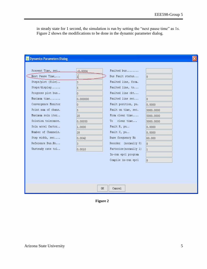
in steady state for 1 second, the simulation is run by setting the “next pause time” as 1s.

Figure 2 shows the modifications to be done in the dynamic parameter dialog.

Figure 2

EEE598-Group 5


Fault simulation: A fault is applied at bus #5. This step is used to determine the

critical clearing time by trial and error method. In this step, the “faulted bus” is first set

to 5 and the “bus fault status” is changed to 1; which means there is a three phase fault

on bus # 5. The “next pause time” is changed to (1+n/60), where n is the number of

cycles for which the fault is applied. A number of simulations were performed by

varying „n‟ between 4 and 5 cycles and the corresponding rotor angle plots are

observed to determine the critical clearing time for a 3-phase short circuit at bus # 5.

The changes made in the dynamic parameters are shown in Figure 3.

Figure 3

EEE598-Group 5


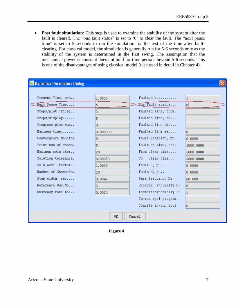
Post fault simulation: This step is used to examine the stability of the system after the

fault is cleared. The “bus fault status” is set to „0‟ to clear the fault. The “next pause

time” is set to 5 seconds to run the simulation for the rest of the time after fault-

clearing. For classical model, the simulation is generally run for 5-6 seconds only as the

stability of the system is determined in the first swing. The assumption that the

mechanical power is constant does not hold for time periods beyond 5-6 seconds. This

is one of the disadvantages of using classical model (discussed in detail in Chapter 4).

Figure 4

EEE598-Group 5


After completing the simulation, the “plot” feature is used to view the plots of all the four rotor

angles.480 628 3960

PSLF makes use of relative plots with reference to the bus at the far end from the fault by

default. In this case, bus # 3 is automatically chosen as the reference because it is the located

both physically and electrically farthest from bus # 5 (faulted bus); shown clearly in Appendix

3.

Figure 5

EEE598-Group 5


Section 3.1 shows the relative rotor angle plot obtained when the three phase fault at bus# 5 is

cleared after 4.3 cycles and 4.4 cycles.

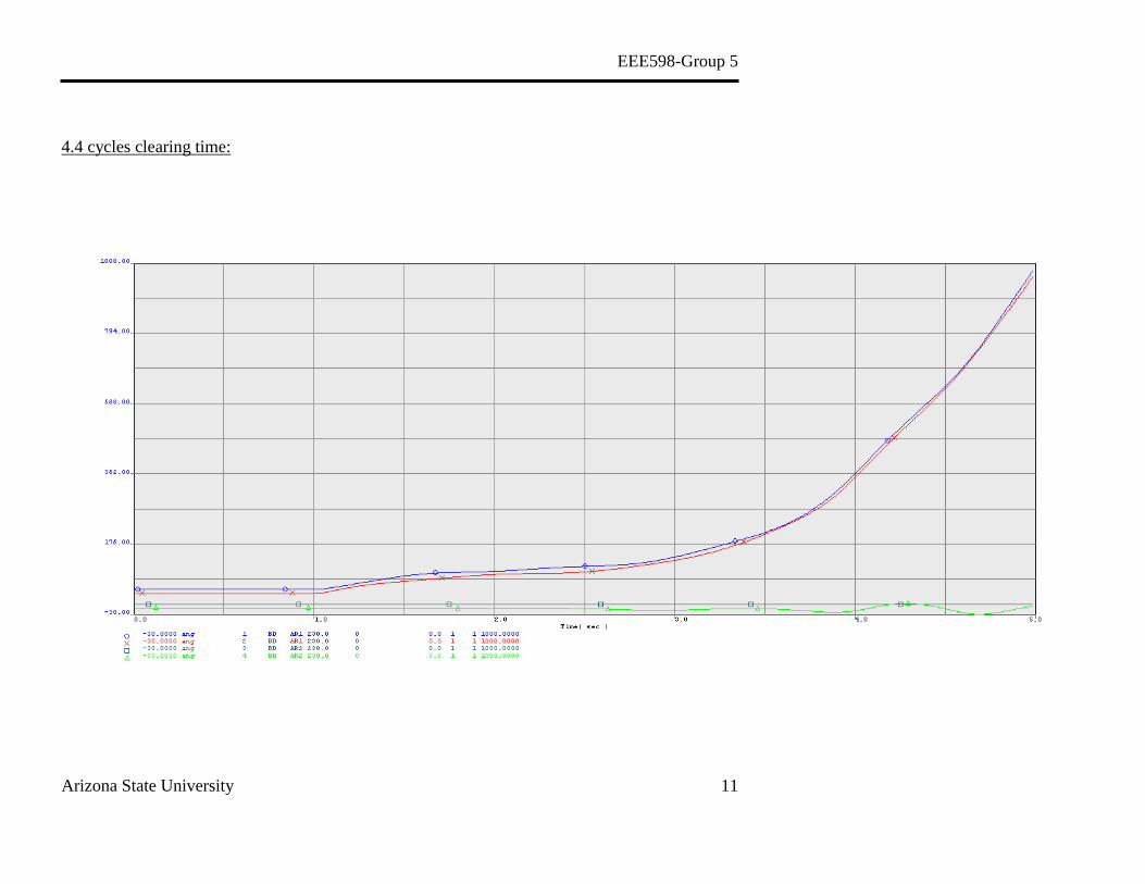
The angle plots for 4.3 cycles show that the machines are operating in synchronism (angles

return back). But in case of 4.4 cycles, the angles grow infinitely even after fault is cleared

(unstable system).

Thus, it is found that the system just losses synchronism when the fault is applied for 4.4

cycles. This means that when the fault is applied for 4.3 cycles, the system is at the edge of

instability; which is the critical clearing time for this system.

It is not possible to plot the absolute rotor angles with the help of PSLF as it is basically

relative software. Also ab

EEE598-Group 5


3.1 Relative Rotor Angles Plots

4.3 cycles clearing time:

EEE598-Group 5


4.4 cycles clearing time:

EEE598-Group 5


4. Shortcomings of Classical Model

The assumptions made for classical model [4] are as follows:

1) Transient stability is decided in the first swing.

2) Constant generator main field-winding flux linkage.

3) Neglecting the damping powers.

4) Constant mechanical power.

5) Representing loads by constant passive impedance.

But today, large system interconnections with the greater system inertias and relatively weaker

ties result in longer periods of oscillations during transients. Generator control systems,

particularly modern excitation systems, are extremely fast. Also, the assumption that the

mechanical power is constant does not hold for greater time periods.

In short, the classical model is inadequate for system representation beyond the first swing.

Since the first swing is largely an inertial response to a given accelerating torque, the classical

model does provide useful information as to system response during this brief period.

5. Inference

Based on the simulation results presented in the previous sections, the following observations

can be made:

The critical clearing time for the given system for a 3 phase fault at bus #5 is 4.3 cycles.

The relative rotor angle plots give a better measure of the loss of synchronism than the

absolute rotor angles because of the following reasons:

o Most of the power flow softwares use this option by default.

o Synchronism is a measure of how close the machines operate with one another;

which means the performance of a machine is measured with respect to another

one. This is the concept behind relative angle plot.

o This is the reason why relative angles are used in industrial standards as well.

EEE598-Group 5


6. References

[1] Power flow raw file, “2area.raw”, EEE598, Fall 2011.

[2] Detailed Dynamic data file, “dyn.dat”, EEE598, Fall 2011.

[3] PSLF User Manual

[4] “Power System Control and Stability” by P.M. Anderson and A.A. Fouad

EEE598-Group 5

Arizona State University i

Appendix 1 PSLF Power Flow Mismatch

Appendix 1 EEE598-Group 5

Arizona State University ii

It -P-error- --Bus-- ----Name---- --Kv-- area -Q-error- --Bus-- ----Name---- --Kv-- area

-delta-A- --Bus-- ----Name---- --Kv-- area -delta-V- --Bus-- ----Name---- --Kv-- area

0 0.0029 6 B L 230.00 2 -0.0004 6 B L 230.00 2

0.0233 2 BD AR1 230.00 1 0.000015 6 B L 230.00 2

1 -0.0000 5 B L 230.00 1 -0.0000 6 B L 230.00 2

0.0000 5 B L 230.00 1 0.000000 6 B L 230.00 2

Stopped after 2 iterations

Estimated solution error 0.0002 MW, 0.0005 MVAR

at buses 5 B L 230.00 6 B L 230.00

Actual mismatch is = -0.0001 MW -0.0004 MVAR at bus 5 [B L ] 230.00

EEE598-Group 5

Arizona State University iii

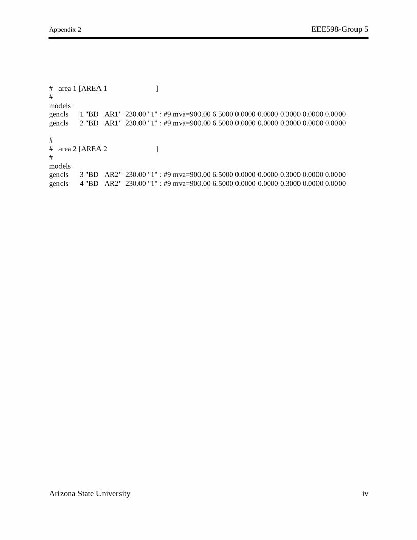
Appendix 2 PSLF Dynamic Data File


Arizona State University iv

# area 1 [AREA 1 ]

#

models

gencls 1 "BD AR1" 230.00 "1" : #9 mva=900.00 6.5000 0.0000 0.0000 0.3000 0.0000 0.0000

gencls 2 "BD AR1" 230.00 "1" : #9 mva=900.00 6.5000 0.0000 0.0000 0.3000 0.0000 0.0000

#

# area 2 [AREA 2 ]

#

models

gencls 3 "BD AR2" 230.00 "1" : #9 mva=900.00 6.5000 0.0000 0.0000 0.3000 0.0000 0.0000

gencls 4 "BD AR2" 230.00 "1" : #9 mva=900.00 6.5000 0.0000 0.0000 0.3000 0.0000 0.0000

EEE598-Group 5

Arizona State University v

Appendix 3 One Line Diagram


Arizona State University vi

BUS# 1

BUS# 2

BUS# 5

BUS# 3

BUS# 4

BUS# 6

ZL_12= 0.0025 + j0.025

ZL_25=0.001 + j0.01

ZL_56=0.022 + j0.22

ZL_64=0.004 + j0.01

ZL_43=0. 0025 + j0.025

Zt_15= 0.0035 + j0.035

Zt_53= 0.0285 + j0.255

GEN1

GEN

2

GEN4

GEN3

Loads

Loads

Eee598 Project New

Documents

Transcript of Eee598 Project New