Eﬀects of Noise on Nonlinear Dynamicsmatrhc/documents/Longtin-noiseinneuralsystems.pdf · 6...

6

Effects of Noise on NonlinearDynamicsAndre Longtin

6.1 Introduction

The influence of noise on nonlinear dynamical systems is a very importantarea of research, since all systems, physiological and other, evolve in thepresence of noisy driving forces. It is often thought that noise has only ablurring effect on the evolution of dynamical systems. It is true that thatcan be the case, especially for so-called “observational” or “measurement”noise, as well as for linear systems. However, in nonlinear systems withdynamical noise, i.e., with noise that acts as a driving term in the equa-tions of motion, noise can drastically modify the deterministic dynamics.For example, the hallmark of nonlinear behavior is the bifurcation, whichis a qualitative change in the phase space motion when the value of one ormore parameter changes. Noise can drastically modify the dynamics of adeterministic dynamical system. It can make the determination of bifurca-tion points very difficult, even for the simplest bifurcations. Noise can shiftbifurcation points or induce behaviors that have no deterministic counter-part, through what are known as noise-induced transitions (Horsthemkeand Lefever 1984). The combination of noise and nonlinear dynamics canalso produce time series that are easily mistakable for deterministic chaos.This is especially true in the vicinity of bifurcation points, where the noisehas its greatest influence.

This chapter considers these issues starting from a basic level of descrip-tion: the stochastic differential equation. It discusses sources of noise, andshows how noise, or “stochastic processes,” can be coupled to determin-istic differential equations. It also discusses analytical tools to deal withstochastic differential equations, as well as simple methods to numericallyintegrate such equations. It then focuses in greater detail on trying to pin-point a Hopf bifurcation in a real physiological system, which will lead tothe notion of a noise-induced transition. This system is the human pupillight reflex. It has been studied by us and others both experimentally and

150 Longtin

theoretically. It is also the subject of Chapter 9, by John Milton; he hasbeen involved in the work presented here, along with Jelte Bos (who car-ried out some of the experiments at the Free University of Amsterdam)and Michael Mackey. This chapter then considers noise-induced firing inexcitable systems, and how noise interacts with deterministic input such asa sine wave to produce various forms of “stochastic phase locking.”

Noise is thought to arise from the action of a large number of variables.In this sense, it is usually understood that noise is high-dimensional. Themathematical analysis of noise involves associating a random variable withthe high-dimensional physical process causing the noise. For example, fora cortical cell receiving synaptic inputs from ten thousand other cells, theongoing synaptic bombardment may be considered as a source of currentnoise. The firing behavior of this cell may then be adequately described byassuming that the model differential equations governing the excitabilityof this cell (e.g., Hodgkin–Huxley-type equations) are coupled to a randomvariable describing the properties of this current noise.

Although we may consider these synaptic inputs as noise, the cell mayactually make more sense of it than we can, such as in temporal and spatialcoincidences of inputs. Hence, one person’s noise may be another person’sinformation: It depends ultimately on the phenomena you are trying tounderstand. This explains in part why there has been such a thrust in thelast decades to discover simple low-dimensional deterministic laws (such aschaos) governing observed noisy fluctuations.

From the mathematical standpoint, noise as a random variable is a quan-tity that fluctuates aperiodically in time. To be a useful quantity to describethe real world, this random variable should have well-defined propertiesthat can be measured experimentally, such as a distribution of values (adensity) with a mean and other moments, and a two-point correlation func-tion. Thus, although the variable itself takes on a different set of valuesevery time we look at it or simulate it (i.e., for each of its “realizations” ), itsstatistical and temporal properties remain constant. The validity of theseassumptions in a particular experimental setting must be properly assessed,for example by verifying that certain stationarity criteria are satisfied.

One of the difficulties with modeling noise is that in general, we do nothave access to the noise variable itself. Rather, we usually have access to astate variable of a system that is perturbed by one or more sources of noise.Thus, one may have to begin with assumptions about the noise and its cou-pling to the dynamical state variables. The accuracy of these assumptionscan later be assessed by looking at the agreement of the predictions of theresulting model with the experimental data.

6. Effects of Noise on Nonlinear Dynamics 151

6.2 Different Kinds of Noise

There is a large literature on the different kinds of noise that can arise inphysical and physiological systems. Excellent references on this subject canbe found in Gardiner (1985) and Horsthemke and Lefever (1984). An excel-lent reference for noise at the cellular level is the book by DeFelice (1981).These books provide background material on thermal noise (also known asJohnson–Nyquist noise, fluctuations that are present in any system due toits temperature being higher than absolute zero), shot noise (due to themotion of individual charges), 1/fα noise (one-over-f noise or flicker noise,the physical mechanisms of which are still the topic of whole conferences),Brownian motion, Ornstein–Uhlenbeck colored noise, and the list goes on.

In physiology, an important source of noise consists of conductance fluc-tuations of ionic channels, due to the (apparently) random times at whichthey open and close. There are many other sources of noise associated withchannels (DeFelice 1981). In a nerve cell, noise from synaptic events canbe more important than the intrinsic sources of noise such as conductancefluctuations. Electric currents from neighboring cells or axons are a form ofnoise that not only affects recordings through measurement noise but alsoa cell’s dynamics. There are fluctuations in the concentrations of ions andother chemicals forming the milieu in which the cells live. These fluctua-tions may arise on a slower time scale than the other noises mentioned upto now.

The integrated electrical activity of nerve cells produces the electroen-cephalogram (EEG) pattern with all its wonderful classes of fluctuations.Similarly, neuromuscular systems are complex connected systems of neu-rons, axons, and muscles, each with its own sources of noise. Fluctuationsin muscle contraction strength are dependent to a large extent on the firingpatterns of the motorneurons that drive them. All these examples shouldconvince you that the modeling of noise requires a knowledge of the basicphysical processes governing the dynamics of the variables we measure.

There is another kind of distinction that must be applied, namely, thatbetween observational, additive, and multiplicative noise (assuming a sta-tionary noise). In the case of observational noise, the dynamical systemevolves deterministically, but our measurements on this system are con-taminated by noise. For example, suppose a one-dimensional dynamicalsystem is governed by

dx

dt= f(x, µ), (6.1)

where µ is a parameter. Then observational noise corresponds to the mea-surement of y(t) ≡ x(t)+ξ(t), where ξ(t) is the observational noise process.The measurement y, but not the evolution of the system x, is affected bythe presence of noise. While this is often an important source of noise withwhich analyses must contend, and the simplest to deal with mathemati-

152 Longtin

cally, it is also the most boring form of noise in a physical system: It doesnot give rise to any new effects.

One can also have additive sources of noise. These situations arecharacterized by noise that is independent of the precise state of the system:

dx

dt= f(x, µ) + ξ(t) . (6.2)

In other words, the noise is simply added to the deterministic part of thedynamics. Finally, one can have multiplicative noise, in which the noise isdependent on the value of one or many state variables. Suppose that f isseparable into a deterministic part and a stochastic part that depends onx:

dx

dt= h(x) + g(x)ξ(t) . (6.3)

We then have the situation where the effect of the noise term will dependon the value of the state variable x through g(x). Of course, a given systemmay have one or more noise sources coupled in one or more of these ways.We will discuss such sources of noise in the context of our experiments onthe pupil light reflex and our study of stochastic phase locking.

6.3 The Langevin Equation

Modeling the precise effects of noise on a dynamical system can be verydifficult, and can involve a lot of guesswork. However, one can alreadygain insight into the effect of noise on a system by coupling it addi-tively to Gaussian white noise. This noise is a mathematical constructthat approximates the properties of many kinds of noise encountered inexperimental situations. It is Gaussian distributed with zero mean andautocorrelation 〈ξ(t)ξ(s)〉 = 2Dδ(t − s), where δ is the Dirac delta func-tion. The quantity D ≡ σ2/2 is usually referred to as the intensity ofthe Gaussian white noise (the actual intensity with the autocorrelationscaling used in our example is 2D). Strictly speaking, the variance of thisnoise is infinite, since it is equal to the autocorrelation at zero lag (i.e. att = s). However, its intensity is finite, and σ times the square root of thetime step will be the standard deviation of Gaussian random numbers usedto numerically generate such noise (see below).

The Langevin equation refers to the stochastic differential equationobtained by adding Gaussian white noise to a simple first-order lineardynamical system with a single stable fixed point:

dx

dt= −αx+ ξ(t) . (6.4)

This is nothing but equation (6.2) with f(x, µ) = −αx, and ξ(t) givenby the Gaussian white noise process we have just defined. The stochastic


process x(t) is also known as Ornstein–Uhlenbeck noise with correlationtime 1/α, or as lowpass-filtered Gaussian white noise. A noise processthat is not white noise, i.e. that does not have a delta-function auto-correlation, is called “colored noise”. Thus, the exponentially correlatedOrnstein–Uhlenbeck noise is a colored noise. The probability density ofthis process is given by a Gaussian with zero mean and variance σ2/2α(you can verify this using the Fokker–Planck formalism described below).In practical work, it is important to distinguish between this variance, andthe intensity D of the Gaussian white noise process used to produce it.It is in fact common to plot various quantities of interest for a stochasticdynamical system as a function of the intensity D of the white noise usedin that dynamical system, no matter where it appears in the equations.

The case in which the deterministic part is nonlinear yields a nonlinearLangevin equation, which is the usual interesting case in mathematicalphysiology. One can simulate a nonlinear Langevin equation with deter-ministic flow h(x, t, µ) and a coefficient g(x, t, µ) for the noise process usingvarious stochastic numerical integration methods of different orders of pre-cision (see Kloeden, Platen, and Schurz 1991 for a review). For example, onecan use a simple “stochastic” Euler–Maruyama method with fixed time step∆t (stochastic simulations are much safer with fixed step methods). Usingthe definition of Gaussian white noise ξ(t) as the derivative of the Wienerprocess W (t) (the Wiener process is also known as “Brownian motion”),this method can be written as

x(t+ ∆t) = x(t) + ∆t h(x, t, µ) + g(x, t, µ)∆Wn , (6.5)

where the {∆Wn} are “increments” of the Wiener process. These incre-ments can be shown to be independent Gaussian random variables withzero mean and standard deviation given by σ

√∆t. Because the Gaussian

white noise ξ(t) is a function that is nowhere differentiable, one must useanother kind of calculus to deal with it (the so-called stochastic calcu-lus; see Horsthemke and Lefever 1984; Gardiner 1985). One consequence ofthis fact is the necessity to exercise caution when performing a nonlinearchange of variables on stochastic differential equations: The “Stratonovich”stochastic calculus obeys the laws of the usual deterministic calculus, butthe “Ito” stochastic calculus does not. One thus has to associate an Itoor Stratonovich interpretation with a stochastic differential equation be-fore performing coordinate changes. Also, for a given stochastic differentialequation, the properties of the random process x(t) such as its momentswill depend on which calculus is assumed. Fortunately, there is a simpletransformation between the Ito and Stratonovich forms of the stochasticdifferential equation. Further, the properties obtained with both calculi areidentical when the noise is additive.

It is also important to associate the chosen calculus with a proper in-tegration method (Kloeden, Platen, and Schurz 1991). For example, anexplicit Euler–Maruyama scheme is an Ito method, so numerical results

154 Longtin

with this method will agree with any theoretical results obtained from ananalysis of the Ito interpretation of the stochastic differential equation, orof its equivalent Stratonovich form. In general, the Stratonovich form isbest suited to model “real colored noise” and its effects in the limit of van-ishing correlation time, i.e. in the limit where colored noise is allowed tobecome white after the calculation of measurable quantities.

Another consequence of the stochastic calculus is that in the Euler–Maruyama numerical scheme, the noise term has a magnitude proportionalto the square root of the time step, rather than to the time step itself. Thismakes this method an “order 1

2” method, which converges more slowly thanthe Euler algorithm for deterministic differential equations. Higher-ordermethods are also available (Fox, Gatland, Roy, and Vemuri 1988; Mannellaand Palleschi 1989; Honeycutt 1992); some are used in the computer exer-cises associated with this chapter and with the chapter on the pupil lightreflex (Chapter 9). Such methods are especially useful for stiff stochasticproblems, such as the Hodgkin–Huxley or FitzHugh–Nagumo equationswith stochastic forcing, where one usually uses an adaptive method in thenoiseless case, but is confined to a fixed step method with noise. Stochasticsimulations usually require multiple long runs (“realizations”: see below)to get good averaging, and higher-order methods are useful for that as well.

The Gaussian random numbers ∆Wn are generated in an uncorrelatedfashion, for example by using a pseudorandom number generator in combi-nation with the Box–Muller algorithm. Such algorithms must be “seeded,”i.e., provided with an initial condition. They will then output numberswith very small correlations between themselves. A simulation that usesGaussian numbers that follow one initial seed is called a realization. In cer-tain problems, it is important to repeat the simulations using M differentrealizations of N points (i.e., M with different seeds). This performs anaverage of the stochastic differential equation over the distribution of therandom variable. It also serves to reduce the variance of various statisticalquantities used in a simulation (such as power spectral amplitudes). In thecase of very long simulations, it also avoids problems associated with thefinite period of the random number generator.

A stochastic simulation yields a different trajectory for each differentseed. It is possible also to describe the action of noise from another pointof view, that of probability densities. One can study, for example, how anensemble of initial conditions, characterized by a density, propagates underthe action of the stochastic differential equation. One can study also theprobability density of measuring the state variable between x and x+dx ata given time. The evolution of this density is governed by a deterministicpartial differential equation in the density variable ρ(x, t), known as theFokker–Planck equation. In one dimension, this equation is

∂ρ

∂t=

12∂2[g2(x)ρ

]∂x2 − ∂ [h(x)ρ]

∂x. (6.6)


Setting the left-hand side to zero and solving the remaining ordinary differ-ential equation yields the asymptotic density for the stochastic differentialequation, ρ∗ = ρ(x,∞). This corresponds to the probability density offinding the state variable between x and x+ dx once transients have diedout, i.e., in the long-time limit. Since noisy perturbations cause transients,this long-time density somehow characterizes not only the deterministic at-tractors, but also the noise-induced transients around these attractors. Forsimple systems, it is possible to calculate ρ∗, and sometimes even ρ(x, t)(this can always be done for linear systems, even with time-dependent co-efficients). However, for nonlinear problems, in general one can at bestapproximate ρ∗. For delay differential equations such as the one studied inthe next section, the Fokker–Planck formalism breaks down. Nevertheless,it is possible to calculate ρ∗ numerically, and even understand some of itsproperties analytically (Longtin, Milton, Bos, and Mackey 1990; Longtin1991a; Guillouzic, L’Heureux, and Longtin 1999).

A simple example of a nonlinear Langevin equation is

dx

dt= x− x3 + ξ(t) , (6.7)

which models the overdamped noise-driven motion of a particle in a bistablepotential. The deterministic part of this system has three fixed points, anunstable one at the origin and stable ones at ±1. For small noise intensityD, the system spends a long time fluctuating on either side of the originbefore making a switch to the other side, as shown in Figure 6.1. Increasingthe noise intensity increases the frequency of the switches across the origin.At the same time, the asymptotic probability density broadens aroundthe stable points, and the probability density in a neighborhood of the(unstable) origin increases; the vicinity of the origin is thus stabilized bynoise. One can actually calculate this asymptotic density exactly for thissystem using the Fokker–Planck formalism (try it! the answer is ρ(x) =C exp

[(x2 − x4)/2D

], where C is a normalization constant). Also, because

this is a one-dimensional system with additive noise, the maxima of thedensity are always located at the same place as for the deterministic case.The maxima are not displaced by noise, and no new maxima are created;in other words, there are no noise-induced states. This is not always thecase for multiplicative noise, or for additive or multiplicative noise in higherdimensions.

6.4 Pupil Light Reflex: Deterministic Dynamics

We illustrate the effect of noise on nonlinear dynamics by first consideringhow noise alters the behavior of a prototypical physiological control system.The pupil light reflex, which is the focus of Chapter 9, is a negative feedbackcontrol system that regulates the amount of light falling on the retina. The

156 Longtin

A B

C D

3

2

1

0

-1

-2

-3

0.8

0.6

0.4

0.2

00 100 200 -4 -2 0 2 4

Time X

Pro

babi

lity

X

3

2

1

0

-1

-2

-3

0.8

0.6

0.4

0.2

00 100 200 -4 -2 0 2 4

Time X

Pro

babi

lity

X

Figure 6.1. Realizations of equation (6.7) at (A) low noise intensity D = 0.5and (C) high noise intensity D = 1.0. The corresponding normalized probabilitydensities are shown in (B) and (D) respectively. These densities were obtainedfrom 30 realizations of 400,000 iterates; the integration time step for the stochasticEuler method is 0.005.

pupil is the hole in the middle of the colored part of the eye called theiris. If the ambient light falling on the pupil increases, the reflex responsewill contract the iris sphincter muscle, thus reducing the area of the pupiland the light flux on the retina. The delay between the variation in lightintensity and the variation in pupil area is about 300 msec. A mathematicalmodel for this reflex is developed in Chapter 9. It can be simplified to thefollowing form:

dA

dt= −αA+

c

1 +[

A(t−τ)θ

]n + k, (6.8)

where A(t) is the pupil area, and the second term on the right is a sigmoidalnegative feedback function of the area at a time τ = 300 msec in the past.Also, α, θ, c, k are constants, although in fact, c and k fluctuate noisily. Theparameter n controls the steepness of the feedback around the fixed point,


A B

C D

2000

1000

0

-1000

-2000

2000

1000

0

-1000

-20000 5 10 15 20

Pup

il ar

ea (

arb.

uni

ts)

2000

1000

0

-1000

-2000

2000

1000

0

-1000

-20000 5 10 15 20

Time (s)

0 5 10 15 20

0 5 10 15 20

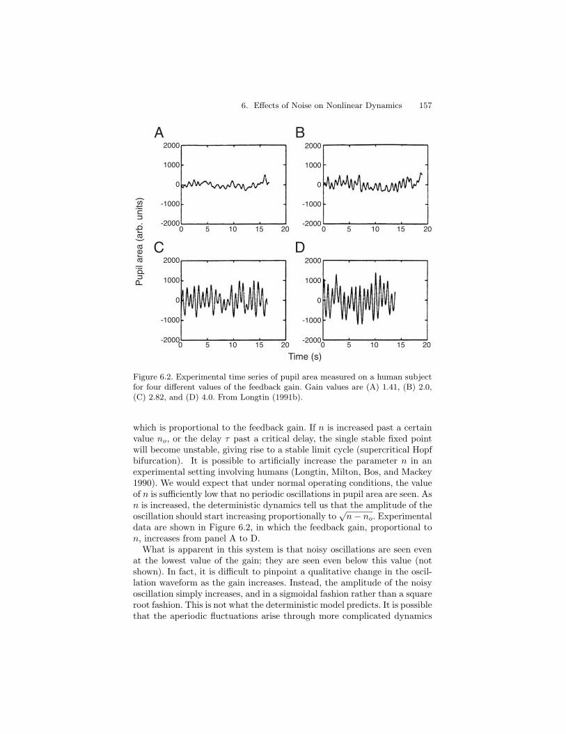
Figure 6.2. Experimental time series of pupil area measured on a human subjectfor four different values of the feedback gain. Gain values are (A) 1.41, (B) 2.0,(C) 2.82, and (D) 4.0. From Longtin (1991b).

which is proportional to the feedback gain. If n is increased past a certainvalue no, or the delay τ past a critical delay, the single stable fixed pointwill become unstable, giving rise to a stable limit cycle (supercritical Hopfbifurcation). It is possible to artificially increase the parameter n in anexperimental setting involving humans (Longtin, Milton, Bos, and Mackey1990). We would expect that under normal operating conditions, the valueof n is sufficiently low that no periodic oscillations in pupil area are seen. Asn is increased, the deterministic dynamics tell us that the amplitude of theoscillation should start increasing proportionally to

√n− no. Experimental

data are shown in Figure 6.2, in which the feedback gain, proportional ton, increases from panel A to D.

What is apparent in this system is that noisy oscillations are seen evenat the lowest value of the gain; they are seen even below this value (notshown). In fact, it is difficult to pinpoint a qualitative change in the oscil-lation waveform as the gain increases. Instead, the amplitude of the noisyoscillation simply increases, and in a sigmoidal fashion rather than a squareroot fashion. This is not what the deterministic model predicts. It is possiblethat the aperiodic fluctuations arise through more complicated dynamics

158 Longtin

A B

C D

60

50

40

30

0.8

0.6

0.4

0.2

030 40 50

Time X

Pro

babi

lity

Pup

il ar

ea

60

50

40

30

0.8

0.6

0.4

0.2

0

Time X

Pro

babi

lity

Pup

il ar

ea

600 10 20 30 40

30 40 50 600 10 20 30 40

Figure 6.3. Characterization of pupil area fluctuations obtained from numericalsimulations of equation (6.8) with multiplicative Gaussian colored noise on theparameter k; the intensity is D = 15, and the noise correlation time is α−1 = 1.The bifurcation parameter is n; a Hopf bifurcation occurs (for D = 0) at n = 8.2.(A) Realization for n = 4; the corresponding normalized probability density isshown in (B). (C) and (D) are the same as, respectively, (A) and (B) but forn = 10. The densities were computed from 10 realizations, each of duration equalto 400 delays.

(e.g., chaos) in this control system. However, such dynamics are not presentin the deterministic model for any combination of parameters and initialconditions. In fact, there are only two globally stable solutions, either afixed point or a limit cycle.

Another possibility is that noise is present in this reflex, and what we areseeing is the result of noise driving a system in the vicinity of a Hopf bifur-cation. This would not be surprising, since the pupil has a well-documentedsource of fluctuations known as pupillary hippus. It is not known what theprecise origin of this noise is, but the following section will show that wecan test for certain hypotheses concerning its nature. Incorporating noiseinto the model can in fact produce fluctuations that vary similarly to thosein Figure 6.2 as the feedback gain is increased, as we will now see.


6.5 Pupil Light Reflex: Stochastic Dynamics

We can explain the behaviors seen in Figure 6.2 if noise is incorporatedinto our model. One can argue, based on the known physiology of thissystem (see Chapter 9), that noise enters the reflex pathway through theparameters c and k, and causes fluctuations about their mean values c andk, respectively. In other words, we can suppose that c = c+ η(t), i.e., thatthe noise is multiplicative, or k = k + η(t), i.e., that the noise is additive,or both. This noise represents the fluctuating neural activity from manydifferent areas of the brain that connect to the Edinger–Westphal nucleus,the neural system that controls the parasympathetic drive of the iris. It alsois meant to include the intrinsic noise at the synapses onto this nucleus andelsewhere in the reflex arc.

Without noise, equation (6.8) undergoes a supercritical Hopf bifurcationas the gain is increased via the parameter n. We have investigated both theadditive and multiplicative noise hypotheses by performing stochastic sim-ulations of equation (6.8). The noise was chosen to be Ornstein–Uhlenbecknoise with a correlation time of one second (Longtin, Milton, Bos, andMackey 1990). Some results are shown in Figure 6.3, where a transitionfrom low amplitude fluctuations to more regular high-amplitude fluctua-tions is seen as the feedback gain is increased. Results are similar with noiseon either c or k. Even before the deterministic bifurcation, oscillations withroughly the same period as the limit cycle that appears at the bifurcationare excited by the noise. Increasing the gain just makes them more promi-nent: In fact, there is no actual bifurcation when noise is present, only agraded appearance of oscillations.

6.6 Postponement of the Hopf Bifurcation

We now discuss the problem of pinpointing a Hopf bifurcation in the pres-ence of noise. This is a difficult problem not only for the Hopf bifurcation,but for other bifurcations as well (Horsthemke and Lefever 1984). Fromthe time series point of view, noise causes fluctuations on the deterministicsolution that exists without noise. However, and this is the more interestingeffect, it can also produce noisy versions of behaviors that occur nearby inparameter space for the noiseless system. For example, as we have seen inthe previous section, near a Hopf bifurcation the noise will produce a mix-ture of fixed-point and limit cycle solutions. In the most exciting examplesof the effect of noise on nonlinear dynamics, even new behaviors having nodeterministic counterpart can be produced.

The problem of pinpointing a bifurcation in the presence of noise arisesbecause there is no obvious qualitative change in dynamics from the timeseries point of view, in contrast with the deterministic case. The definition

160 Longtin

of a bifurcation as a qualitative change in the dynamical behavior when aparameter is varied has to be modified for a noisy system. There is usuallymore than one way of doing this, depending on which order parameterone chooses, i.e., which aspect of the dynamics one focuses on; the locationof the bifurcation may also depend on this choice of order parameter.

In the case of the pupil light reflex near a Hopf bifurcation, it is clearfrom Figure 6.3 that noise causes oscillations even though the deterministicbehavior is a fixed point. The noise is simply revealing the behavior beyondthe Hopf bifurcation. It is as though noise causes the bifurcation parameterto fluctuate across the deterministic bifurcation. This is a useful way tovisualize the effect of noise, but it may be misleading, since the parameterneed not fluctuate across the bifurcation point to see a mixture of behaviorsbelow and beyond this point. One can thus say, from the time series pointof view, that noise advances the bifurcation point, since (noisy) oscillationsare seen where, deterministically, a fixed point should be seen. Further, onecan compare features of the noisy oscillation in time with, for example, thesame features predicted by a model (see below).

This analysis has its limitations, however, because power spectral (orautocorrelation) measures of the strength of the oscillatory component ofthe time series do not exhibit a qualitative change as parameters (includingnoise strength) vary. Rather, for example, the peak in the power spectrumassociated with the oscillation simply increases as the underlying determin-istic bifurcation is approached or the noise strength is increased. In otherwords, there is no bifurcation from the spectral point of view. Also, thispoint of view does not necessarily give a clear picture of the behavior be-yond the deterministic bifurcation. For example, can one say that the fixedpoint, which is unstable beyond the deterministic bifurcation, is stabilizedby noise? In other words, does the system spend more time near the fixedpoint than without noise? This can be an important piece of informationabout the behavior of a real control system (see also Chapter 8 on cellreplication and control).

There are measures that reveal a bifurcation in the noisy system. Onemeasure is based on the computation of invariant densities for the solutions.In other words, let the solution run long enough so that transients havedisappeared, and then build a histogram of values of the solution. It isbetter to repeat this process for many realizations of the stochastic processin order to obtain a smooth histogram.

In the deterministic case, this will produce two qualitatively differentdensities, depending on whether n is below or above the deterministic Hopfbifurcation point no. If it is below, then the asymptotic solution is a fixedpoint, and the density is a delta function at this fixed point: ρ∗(x) =δ(x − x∗). If n > no, the solution is approximately a sine wave, for which


the density is

ρ∗(x) =1

πA cos [arcsin(x/A)], (6.9)

where A is the amplitude of the sine wave.When the noise intensity is greater than zero, the delta function gets

broadened to a Gaussian distribution, and the density for the sine wavegets broadened to a smooth double-humped or bimodal function. Exam-ples are shown in Figure 6.3 for two values of the feedback parameter n. Itis possible then to define the bifurcation in the stochastic context by thetransition from unimodality to bimodality (Horsthemke and Lefever 1984).The distance between the peaks can serve as an order parameter for thistransition (different order parameters can be defined, as in the physics liter-ature on phase transitions). It represents in some sense the mean amplitudeof the fluctuations.

We have found that the transition from a unimodal to a bimodal densityoccurs at a value of n greater than no (Longtin, Milton, Bos, and Mackey1990). In this sense, the bifurcation is postponed by the noise, with themagnitude of the postponement being proportional to the noise intensity.In certain simple cases (although not yet for the delay-differential equationstudied here), it is possible to analytically approximate the behavior of theorder parameter with noise. This allows one to predict the presence of apostponement, and to relate this postponement to certain model param-eters, especially those governing the nonlinear behavior. A postponementdoes not imply that there are no oscillations if n < np, where np is the ex-trapolated bifurcation point for the noisy case (it is very time-consumingto numerically determine this point accurately). As we have seen, whenthere is noise near a Hopf bifurcation, oscillations are present. However, apostponement does imply that if n > no, the presence of noise stabilizesthe fixed point. In other words, the system spends more time near the fixedpoint with noise than without noise. This is why the density for the stochas-tic differential equation fills in between the two peaks of the deterministicdistribution given in equation (6.9).

One can try to pinpoint the bifurcation in the pupil data by comput-ing such densities at different values of the feedback gain. The result isshown in Figure 6.4 for the data used for Figure 6.2. Even for the high-est value of gain, there are clearly oscillations, and the distribution stillappears unimodal. However, this is not to say that it is unimodal. A prob-lem arises because a large number of simulated data points (two ordersof magnitude more than experimentally available) are needed to properlymeasure the order parameter, i.e., the distance between the two peaks ofthe probability density. The bifurcation is not seen from the density pointof view in this system with limited data sets and large amounts of noise(the higher the noise, the more data points are required). The model doessuggest, however, that a postponement can be expected from the density

162 Longtin

point of view; in particular, the noisy system spends more time near thefixed point than without noise, even though oscillations occur. Further, themean, moments, and other features of these densities could be comparedto those obtained from time series of similar duration generated by models,in the hope of better understanding the dynamics underlying such noisyexperimental systems.

This lack of resolution to pinpoint the Hopf bifurcation motivated us tovalidate our model using other quantities, such as the mean and relativestandard deviation of the amplitude and period fluctuations as gain in-creases (Longtin, Milton, Bos, and Mackey 1990). That study showed thatfor noise intensity D = 15 and a noise correlation time around one, thesequantities have similar values in the experiments and the simulations. Thisstrengthens our belief that stochastic forces are present in this system. In-terestingly, our approach of investigating fluctuations across a bifurcation(supercritical Hopf in this case) allows us to amplify the noise in the sys-tem, in the sense that it is put under the magnifying glass. This is becausenoise has a strong effect on the dynamics of a system in the vicinity of abifurcation point, since there is loss of linear stability at this point (neitherthe fixed point nor the zero-amplitude oscillation is attracting).

Finally, there is an interesting theoretical aspect to the postponements.We are dealing here with a first-order differential-delay equation. Noise-induced transitions such as postponements are not possible with additivenoise in one-dimensional ordinary differential equations (Horsthemke andLefever 1984). But our numerical results show that in fact, additive noise-induced transitions are possible in a first-order delay-differential equation.The reason behind this is that while the highest-order derivative is one,the delay-differential equation is infinite-dimensional, since it evolves ina functional space (an initial function must be specified). More detailson these theoretical aspects of the noise-induced transitions can be foundin Longtin (1991a).

6.7 Stochastic Phase Locking

The nervous system has evolved with many sources of noise, acting fromthe microscopic ion channel scale up to the macroscopic scale of the EEGactivity. This is especially true for cells that transduce physical stimuli intoneuroelectrical activity, since they are exposed to environmental sources ofnoise, as well as to intrinsic sources of noise such as ionic channel conduc-tance fluctuations, synaptic fluctuations, and thermal noise. Traditionally,sources of noise in sensory systems, such as the senses of audition and touch,have been perceived as a nuisance. For example, they have been thoughtto limit our aptitude for detecting or discriminating between stimuli.


A B

C D

400

300

200

100

0

400

300

200

100

0-2000 -1000 0 1000 2000

Num

ber

of e

vent

s

400

300

200

100

0

150

100

50

0

Pupil area (arb. units)

-2000 -1000 0 1000 2000

-2000 -1000 0 1000 2000-2000 -1000 0 1000 2000

Figure 6.4. Densities corresponding to the time series shown in Figure 6.2 (moredata were used than are shown in Figure 6.2). From Longtin (1991b).

In the past decades, there have been studies that revealed a more con-structive role for neuronal noise. For example, noise can increase thedynamic range of neurons by linearizing their stimulus–response charac-teristics (see, e.g., Spekreijse 1969; Knight 1972; Treutlein and Schulten1985). In other words, noise smoothes out the abrupt increase in mean fir-ing rate that occurs in many neurons as the stimulus intensity increases;this abruptness is a property of the deterministic bifurcation from nonfiringto firing behavior. Noise also makes detection of weak signals possible (see,e.g., Hochmair-Desoyer, Hochmair, Motz, and Rattay 1984). And noisecan stabilize systems by postponing bifurcation points, as we saw in theprevious section (Horsthemke and Lefever 1984).

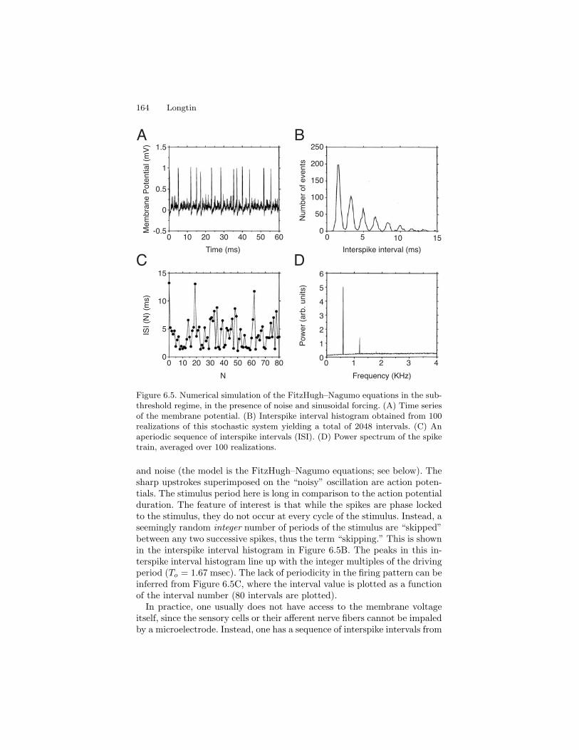
In this section, we focus on a special kind of firing behavior exhibited bymany kinds of neurons across many different sensory modalities. In gen-eral terms, it can be referred to as “stochastic phase locking,” but in morespecific terms it is known as “skipping.” An overview of physiological ex-amples of stochastic phase locking in neurons can be found in Segundo,Vibert, Pakdaman, Stiber, and Martinez (1994). Figure 6.5 plots the mem-brane potential versus time for a model cell driven by a sinusoidal stimulus

164 Longtin

A B

C D

1.5

1

0.5

0

-0.5

250

200

150

100

50

00 5 10

Time (ms) Interspike interval (ms)

Num

ber

of e

vent

s

Mem

bran

e P

oten

tial (

mV

)

15

10

5

0

6

5

4

3

2

1

0

N Frequency (KHz)

Pow

er (

arb.

uni

ts)

ISI (

N)

(ms)

150 10 20 40 60

0 2 3 40 20 40 60 80

30 50

10 30 50 70 1

Figure 6.5. Numerical simulation of the FitzHugh–Nagumo equations in the sub-threshold regime, in the presence of noise and sinusoidal forcing. (A) Time seriesof the membrane potential. (B) Interspike interval histogram obtained from 100realizations of this stochastic system yielding a total of 2048 intervals. (C) Anaperiodic sequence of interspike intervals (ISI). (D) Power spectrum of the spiketrain, averaged over 100 realizations.

and noise (the model is the FitzHugh–Nagumo equations; see below). Thesharp upstrokes superimposed on the “noisy” oscillation are action poten-tials. The stimulus period here is long in comparison to the action potentialduration. The feature of interest is that while the spikes are phase lockedto the stimulus, they do not occur at every cycle of the stimulus. Instead, aseemingly random integer number of periods of the stimulus are “skipped”between any two successive spikes, thus the term “skipping.” This is shownin the interspike interval histogram in Figure 6.5B. The peaks in this in-terspike interval histogram line up with the integer multiples of the drivingperiod (To = 1.67 msec). The lack of periodicity in the firing pattern can beinferred from Figure 6.5C, where the interval value is plotted as a functionof the interval number (80 intervals are plotted).

In practice, one usually does not have access to the membrane voltageitself, since the sensory cells or their afferent nerve fibers cannot be impaledby a microelectrode. Instead, one has a sequence of interspike intervals from


which the mechanisms giving rise to signal encoding and skipping must beinferred.

In the rest of this chapter, we describe some mechanisms of skipping insensory cells, as well as the potential significance of such firing patterns forsensory information processing. We discuss the phenomenology of skippingpatterns, and then describe efforts to model these patterns mathematically.We describe the stochastic resonance effect in this context, and discuss itsorigins. We also discuss skipping patterns in the context of “bursting” firingpatterns. We consider the relation of noise-induced firing to linearizationby noise. We also show how noise can alter the shape of tuning curves, andend with an outlook onto interesting issues for future research.

6.8 The Phenomenology of Skipping

A firing pattern in which cycles of a stimulus are skipped is a commonoccurrence in physiology. For example, this behavior underlies p : m phaselocking seen in cardiac and other excitable cells, i.e., firing patterns with mresponses to p cycles of the stimulus. The main additional properties hereare that the phase locking pattern is aperiodic, and remains qualitativelythe same as stimulus characteristics are varied. In other words, abruptchanges between patterns with different phase locking ratios are not seenunder “skipping” conditions. For example, as the amplitude of the stimulusincreases, the skipping pattern remains aperiodic, but there is a higherincidence of short skips rather than long skips.

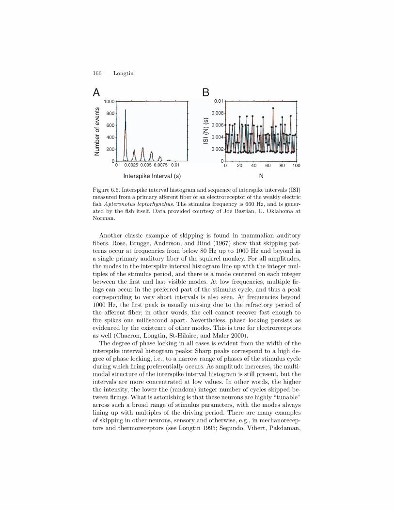
A characteristic interspike interval histogram for a skipping pattern isshown in Figure 6.5B, and again in Figure 6.6A for in a bursty P-typeelectroreceptor of a weakly electric fish. The stimulus in this latter case isa 660 Hz oscillatory electric field generated by the fish itself (its “electricorgan discharge”). It is modulated by food particles and other objects andfish, and the 660 Hz carrier along with its modulations are read by thereceptors in the skin of the fish. This electrosensory system is used for elec-trolocation and electrocommunication. The interspike interval histogramin Figure 6.6A again consists of a set of peaks located at integer multiplesof the driving period. Note from Figure 6.6B that there is no apparentperiodicity in the interval sequence. The firing patterns of electroreceptorswere first characterized in Scheich, Bullock, and Hamstra Jr (1973). Thesereceptors are known are P-units or “probability coders,” since it is thoughtthat their probability of firing is proportional to, and thus encodes, theinstantaneous amplitude of the electric organ discharge. Hence this prob-ability, determined by various parameters including the intensity of noisesources acting in the receptor, is an important part of the neuronal codein this system.

166 Longtin

A B1000

800

600

400

200

0

0.01

0.008

0.006

0.004

0.002

00 0.0025 0.01 0 20 40 60 100

Interspike Interval (s) N

ISI (

N)

(s)

0.005 0.0075 80

Num

ber

of e

vent

s

Figure 6.6. Interspike interval histogram and sequence of interspike intervals (ISI)measured from a primary afferent fiber of an electroreceptor of the weakly electricfish Apteronotus leptorhynchus. The stimulus frequency is 660 Hz, and is gener-ated by the fish itself. Data provided courtesy of Joe Bastian, U. Oklahoma atNorman.

Another classic example of skipping is found in mammalian auditoryfibers. Rose, Brugge, Anderson, and Hind (1967) show that skipping pat-terns occur at frequencies from below 80 Hz up to 1000 Hz and beyond ina single primary auditory fiber of the squirrel monkey. For all amplitudes,the modes in the interspike interval histogram line up with the integer mul-tiples of the stimulus period, and there is a mode centered on each integerbetween the first and last visible modes. At low frequencies, multiple fir-ings can occur in the preferred part of the stimulus cycle, and thus a peakcorresponding to very short intervals is also seen. At frequencies beyond1000 Hz, the first peak is usually missing due to the refractory period ofthe afferent fiber; in other words, the cell cannot recover fast enough tofire spikes one millisecond apart. Nevertheless, phase locking persists asevidenced by the existence of other modes. This is true for electroreceptorsas well (Chacron, Longtin, St-Hilaire, and Maler 2000).

The degree of phase locking in all cases is evident from the width of theinterspike interval histogram peaks: Sharp peaks correspond to a high de-gree of phase locking, i.e., to a narrow range of phases of the stimulus cycleduring which firing preferentially occurs. As amplitude increases, the multi-modal structure of the interspike interval histogram is still present, but theintervals are more concentrated at low values. In other words, the higherthe intensity, the lower the (random) integer number of cycles skipped be-tween firings. What is astonishing is that these neurons are highly “tunable”across such a broad range of stimulus parameters, with the modes alwayslining up with multiples of the driving period. There are many examplesof skipping in other neurons, sensory and otherwise, e.g., in mechanorecep-tors and thermoreceptors (see Longtin 1995; Segundo, Vibert, Pakdaman,


Stiber, and Martinez 1994; Ivey, Apkarian, and Chialvo 1998 and referencestherein).

Another important characteristic of skipping is that the positions ofthe peaks vary smoothly with stimulus frequency, and the envelope ofthe interspike interval histogram varies smoothly with stimulus amplitude.This is different from the phase-locking patterns governed, for example, byphase-resetting curves leading to an Arnold tongue structure as stimulusamplitude and period are varied. We will see that a plausible mechanismfor skipping involves the combination of noise with subthreshold dynamics,although suprathreshold mechanisms exist, as we will see below (Longtin1998). In fact, we have recently found (Chacron, Longtin, St-Hilaire, andMaler 2000) that suprathreshold periodic forcing of a leaky integrate-and-fire model with voltage and threshold reset can produce patterns close tothose seen in electroreceptors of the nonbursty type (interspike intervalhistogram similar to that in Figure 6.6A, except that the first peak is miss-ing). We focus below on the subthreshold scenario in the context of theFitzHugh–Nagumo equations, with one suprathreshold example as well.

6.9 Mathematical Models of Skipping

The earliest analytical/numerical study of skipping was performed by Ger-stein and Mandelbrot (1964). Cat auditory fibers recorded during auditorystimulation with periodic “clicks” of noise (at frequencies less than 100clicks/sec) showed skipping behavior. Gerstein and Mandelbrot were in-terested in reproducing experimentally observed spontaneous interspikeinterval histograms using “random walks to threshold models” of neuronfiring activity. In one of their simulations, they were able to reproduce thebasic features of the interspike interval histogram in the presence of theclicks by adding a periodically modulated drift term to their random walkmodel. The essence of these models is that the firing activity is entirelygoverned by noise plus a constant and/or a periodically modulated drift.A spike is associated with the crossing of a fixed threshold by the randomvariable.

Since this early study, there have been other efforts aimed at under-standing the properties of neurons driven by periodic stimuli and noise.The following examples have been excerpted from the large literature onthis subject. French et al. (1972) showed that noise breaks up patterns ofphase locking to a periodic signal, and that the mean firing rate is propor-tional to the amplitude of the signal. Glass et al. (1980) investigated anintegrate-and-fire model of neural activity in the presence of periodic forc-ing and noise. They found unstable zones with no phase locking, as well asquasi-periodic dynamics and firing patterns with stochastic skipped beats.Keener et al. (1981) were able to analytically investigate the dynamics of

168 Longtin

phase locking in a leaky integrate-and-fire model without noise. Alexanderet al. (1990) studied phase locking phenomena in the FitzHugh–Nagumomodel of a neuron in the excitable regime, again without noise. There havealso been studies of noise-induced limit cycles in excitable cell models likethe Bonhoeffer–van der Pol equations (similar to the FitzHugh–Nagumomodel), but in the absence of periodic forcing (Treutlein and Schulten1985).

The past two decades have seen a revival of stochastic models of neuralfiring in the context of skipping. Hochmair-Desoyer et al. (1984) have lookedat the influence of noise on firing patterns in auditory neurons using modelssuch as the FitzHugh–Nagumo equations, and shown that it can alter thetuning curves (see below). This model generates real action potentials witha refractory period. It also has many other behaviors that are found in realneurons, such as a resonance frequency. It is a suitable model, however, onlywhen an action potential is followed by a hyperpolarizing after-potential,i.e., the voltage goes below the resting potential after the spike, and slowlyincreases towards it. It is also a good simplified model to study certainneural behaviors qualitatively; better models exist (they are usually morecomplex) and should be used when quantitative agreement between theoryand experiment is sought. The study of the FitzHugh–Nagumo model inLongtin (1993) was motivated by the desire to understand how stochasticresonance could occur in real neurons, as opposed to bistable systems wherethe concept had been confined. In fact, the FitzHugh–Nagumo model hasa cubic nonlinearity, just as does the standard quartic bistable system inequation (6.7); however, it has an extra degree of freedom that serves toreset the system after the threshold for spiking is crossed.

We illustrate here the behavior of the FitzHugh–Nagumo model withsimultaneous stimulation by a periodic signal and by noise. The lattercan be interpreted as either synaptic noise, or signal noise, or conduc-tance fluctuations (although the precise modeling of such fluctuations isbetter done with conductance-based models such as Hodgkin–Huxley-typemodels). The model equations are (Longtin 1993)

εdv

dt= v(v − a)(1− v)− w + η(t), (6.10)

dw

dt= v − dw − b− r sinβt, (6.11)

dη

dt= −λη + λξ(t). (6.12)

The variable v is the fast voltage-like variable, while w is a recovery variable.Also, ξ(t) is a zero-mean Gaussian white additive noise, which is lowpassfiltered to produce an Ornstein–Uhlenbeck-type additive noise denoted byη. The autocorrelation of the white noise is 〈ξ(t)ξ(s)〉 = 2Dδ(t − s); i.e.,it is delta-correlated. The parameter D is the intensity of the white noise.This Ornstein–Uhlenbeck noise is Gaussian and exponentially correlated,


with a correlation time (i.e., the 1/e time) of tc = λ−1. The periodic signalof amplitude r and frequency β is added here to the recovery variable was in Alexander, Doedel, and Othmer (1990), yielding qualitatively similardynamics as in the case in which it is added to the voltage equation (afterproper adjustment of the amplitude; see Longtin 1993). The periodic forcingshould be added to the voltage variable when the period of stimulation issmaller than the refractory period of the action potential.

The parameter regime used to obtain the results in Figure 6.5 can beunderstood as follows. In the absence of periodic stimulation, one wouldsee a smooth unimodal interspike interval histogram (close to a gamma-typedistribution) governed by the interaction of the two-dimensional FitzHugh–Nagumo dynamics with noise. The periodic stimulus thus carves peaks outof this “background” distribution of the interspike interval histogram. If thenoise is turned off and the stimulus is turned on, there would be no firingswhatsoever. This is a crucial point: The condition for obtaining skippingwith the tunability properties described in the previous section is that thedeterministic dynamics must be subthreshold. This feature can be controlledby the parameter b, which sets the proximity of the resting potential (i.e.,the single stable fixed point) to the threshold. In fact, this dynamical systemgoes through a supercritical Hopf bifurcation at bH = 0.35. It can also becontrolled by a constant current that could be added to the left hand sideof the first equation.

Figure 6.7 contrasts the subthreshold (r = 0.2) and suprathreshold(r = 0.22) behavior in the FitzHugh–Nagumo system. In the subthresh-old case, the noise is essential for firings to occur: No intervals are obtainedwhen the noise intensity, D, is zero. For r = 0.22 and D = 0, only one kindof interval is obtained, namely, that corresponding to the period of the de-terministic limit cycle. For D > 0, the limit cycle is perturbed by the noise,and sometimes comes close to but misses the separatrix: No action potentialis generated during one or more cycles of the stimulus. In the subthresholdcase, one also sees skipping behavior. At higher noise intensities, the inter-spike interval histograms hardly differ, and thus we cannot tell from suchan interspike interval histogram whether the system is suprathreshold orsubthreshold. This distinction can be made by varying the noise level asillustrated in this figure. In the subthreshold case, the mean of the distri-bution will always move to lower intervals as D increases, although this isnot true for the suprathreshold case.

There have also been numerous modeling studies based on noise andsinusoidally forced integrate-and-fire-type models (see, e.g., Shimokawa,Pakdaman, and Sato 1999; Bulsara, Elston, Doering, Lowen, and Lin-denberg 1996; and Gammaitoni, Hanggi, Jung, and Marchesoni 1998 andreferences therein). Other possible generic dynamical behavior might lurkbehind this form of phase locking. In fact, the details of the phase locking,and of the physiology of the cells, are important in determining which spe-cific dynamics are at work. Subthreshold chaos might be involved (Kaplan,

170 Longtin

D=0

5 6

Subthreshold: r=0.20

1000

500

0

0 1 2 43

Num

ber

of e

vent

s

Suprathreshold: r=0.22

Interspike interval Interspike interval

D=0

D=10-6 D=10-6

D=10-5 D=10-5

5 60 1 2 43

1000

500

0

1000

500

0

Figure 6.7. Comparison of interspike interval histograms with increasing noiseintensity in the subthreshold regime (left panels) and suprathreshold regime (rightpanels).

Clay, Manning, Glass, Guevara, and Shrier 1996), although probably withnoise as well if one seeks smooth interspike interval histograms with sym-metric modes and without missing modes between the first and the last(as with the data in Rose, Brugge, Anderson, and Hind 1967; see Longtin1998). An example of these effects of noise on the multimodal interspikeinterval histograms produced by the chaos (with pulsatile forcing) is shownin Figure 6.8. In other systems, chaos may be the main player, as in theexperimental system (pulsatile stimulation of squid axons) considered inKaplan et al. (1996).

In Figure 10 of Longtin (1993), a “chaos” hypothesis for skipping wasinvestigated using the FitzHugh–Nagumo model with sinusoidal forcing (in-stead of pulses as in Kaplan, Clay, Manning, Glass, Guevara, and Shrier1996). Without noise, this produced subthreshold chaos, as described in Ka-plan, Clay, Manning, Glass, Guevara, and Shrier (1996), although clearly,when spikes occur (using some criterion for graded responses) these are“suprathreshold” responses to this “subthreshold chaos”; in other words,


A B

20

00 100 200 0 100 200

Interspike interval (ms) Interspike interval (ms)

Num

ber

of in

terv

als

Figure 6.8. Interspike interval histogram from the FitzHugh–Nagumo systemdv/dt = v(v − 0.139)(1 − v) − w + I + η(t), dw/dt = 0.008(v − 2.54w), whereI consists of rectangular pulses of duration 1.0 msec and height 0.28, repeatedevery 28.5 msec. Each histogram is obtained from one realization of 5 × 107 timesteps. The Ornstein–Uhlenbeck noise η(t) has a correlation time of 0.001 msec.(A) Noise intensity D = 0. (B) D = 2.5 × 10−5.

the chaos could just as well be referred to as “suprathreshold.” In thisFitzHugh–Nagumo chaos case, some features of the Rose et al. data couldbe reproduced, but others not. For example, multimodal histograms werefound. But the individual peaks had more “internal” structure than seen inthe data (including electroreceptor and mechanoreceptor data); they werenot aligned very well with the integer multiples of the driving period; andsome peaks were missing, as in the case of pulsatile forcing shown in Fig-ure 6.8. Further, the envelope did not have the characteristic exponentialdecay (past the second mode) seen in the Rose et al. data (which is whatis expected for uncorrelated intervals). Additive dynamical noise on topof this chaos did a better job at reproducing these qualitative features, atleast for the parameters explored (Longtin 1998). The modes of the inter-spike interval histogram were still a bit lopsided, and the envelopes weredifferent from those of the data. Interestingly, solutions that “look chaotic”often end up on periodic orbits after a long while. A bit of noise wouldprobably keep these solutions bouncing around irregularly.

The other reason that some stochastic component may be a necessaryingredient is the smoothness observed in the transitions between interspikeinterval histograms as stimulation parameters are changed. Changing pe-riod or amplitude in the chaotic models leads to sometimes abrupt changesin the multimodal structure (and some peaks just keep on missing). Noiseinduced firing with deterministically subthreshold dynamics does producethe required smooth transitions in the proper sequence seen in Rose etal. (1967). Note, however, that in certain parameter ranges, it is possibleto get multimodal histograms with suprathreshold forcing. This is shown

172 Longtin

800

600

400

200

00.50 1.0 1.5

Interspike interval

Num

ber

of e

vent

s

Figure 6.9. Interspike interval histogram from the FitzHugh–Nagumo system withfast sinusoidal forcing β = 32. Other parameters are a = 0.5, b = 0.15, d = 1,ε = 0.005, I = 0.04 and r = 0.06. The histogram is obtained from 10 realizationsof 500,000 time steps.

in Figure 6.9, for which the forcing frequency is high, and the deterministicsolution is a periodic 3:1 solution.

All this discussion does not exclude the possibility that chaos alone (e.g.,with other parameters or in a more refined model) might give the rightpicture for this kind of data, or that deterministic chaos or periodic phaselocking combined with noise might give it as well. Only good intracellulardata can ultimately settle the issue of the origin of the stochastic phaselocking, and provide an explanation for the smooth skipping patterns.

6.10 Stochastic Resonance

The notion that skipping neurons in the subthreshold regime rely on noiseto fire is interesting from the point of view of signal processing. In orderto transmit information about the stimulus (the input) to a neuron in itsspike train (the output), noise must be present. Without noise, there areno firings, and with too much noise, we expect to see a very noisy outputwith again no information (or very little) about the stimulus. Hence, theremust be a noise value for which information about the stimulus is optimallytransmitted to the output. In other words, starting from zero noise, addingnoise will increase the signal-to-noise ratio, and an optimal noise level canbe found where the signal-to-noise ratio peaks. This is indeed the casein the FitzHugh–Nagumo model studied above. This effect, in which thesignal-to-noise ratio is optimal for some intermediate noise intensity, is


known as stochastic resonance. It has been studied for over a decade,usually in bistable systems. It had been studied theoretically in bistableneurons (Bulsara, Jacobs, Zhou, Moss, and Kiss 1991), and predicted tooccur in real neurons (Longtin, Bulsara, and Moss 1991). Thereafter, itwas studied theoretically in an excitable system (Longtin 1993; Chialvoand Apkarian 1993; Chapeau-Blondeau, Godivier, and Chambet 1996) anda variety of other systems (Gammaitoni, Hanggi, Jung, and Marchesoni1998), and shown to occur in real systems (see, e.g., Douglass, Wilkens,Pantazelou, and Moss 1993; Levin and Miller 1996). It is one of manyconstructive roles for noise discovered in recent decades (Astumian andMoss 1998).

This resonance can be studied from the points of view of spectralamplitude at the signal frequency, signal-to-noise ratio, residence-time his-tograms (i.e., interspike interval histograms), and others as well. In the firstcase, one computes for a given value of noise intensity D the power spec-trum averaged over many spike trains obtained with as many realizationsof the noise process. The spectrum is usually in the form of a flat or curvedbackground, on which the harmonics of the small stimulus signal are su-perimposed (see Figure 6.5D). A dip at low frequencies is often seen, whichis due to phase jitter and to the refractory period. A signal-to-noise ratiocan then be computed by dividing the height of the fundamental stimu-lus peak by the noise floor (i.e., the value of the noise background at thefrequency of the stimulus). This signal-to-noise ratio can be plotted as afunction of D, and the resulting curve will be unimodal, with the maximumcorresponding to the stochastic resonance. Alternatively, one can measurethe heights of the different peaks in the interspike interval histogram, andplot these heights as a function of D. The different peaks will go througha maximum at different values of D. While there is yet no direct analyticalconnection between stochastic resonance from these two points of view, itis usually the case that systems exhibiting stochastic resonance from onepoint of view will also exhibit it from the other.

The power spectrum measures the synchrony between firings and thestimulus. From the point of view of the interspike interval histogram, themeasure of synchrony depends not only on the prevalence of intervals atinteger multiples of a fundamental interval, but also on the width of thepeaks of the interspike interval histogram. As noise increases past the res-onance value, these widths increase, with the result that the phase lockingis disrupted by the noise, even though there are many firings.

A simple theory of stochastic resonance for excitable systems is beingdeveloped. Wiesenfeld et al. (1994) have shown that stochastic resonancewill occur in a periodically modulated point process. By redoing the cal-culation of the classic shot noise effect for the case of a periodic stimulus(the point process is then inhomogeneous, i.e., time-dependent), they have

174 Longtin

found an expression for the signal-to-noise ratio (SNR) (in decibels):

SNR = 10 log10

[4I2

1 (z)Io(z)

exp(−U/D)], (6.13)

where In is the modified Bessel function of order n, z ≡ rU/D, and U isa measure of the proximity of the fixed point to the firing threshold (i.e.,some kind of activation barrier). For small z, this equation becomes

SNR = 10 log10

[U2r2

D2 exp(−U/D)], (6.14)

which is almost identical to a well-known result for stochastic resonance in abistable potential. More recently, analytical techniques have been devised tostudy stochastic resonance in two-variable systems such as the FitzHugh–Nagumo system (Lindner and Schimansky-Geier 2000).

The shape of the interspike interval histogram, and in particular, itsrate of decay, is very sensitive to the stimulus characteristics. This is tobe contrasted with the transition from sub- to suprathreshold dynamicsin the absence of noise. There are no firings before the stimulus exceeds athreshold amplitude. Once the suprathreshold regime is reached, however,amplitude increases can bring on various p : m locking patterns and evenchaos. Noise allows the firing pattern to change smoothly and sensitivelyover a larger range of stimulus parameters.

The firing patterns of the neuron in the excitable regime are also inter-esting in the presence of noise only, i.e., without periodic forcing. In fact,such a noisy excitable system can be seen as a stochastic oscillator (Longtin1993; Pikovsky and Kurths 1997; Longtin and Chialvo 1998; Lee and Kim1999; Lindner and Schimansky-Geier 2000). The presence of a resonancein the deterministic dynamics will endow this oscillator with a well-definedpreferred time between firings; this time scale is closely associated withthe period of the limit cycle that arises when the system is biased into itsautonomously firing regime. Recently, Pikovsky and Kurths (1997) showedthat increasing the noise intensity from zero will lead to enhanced period-icity in the output firing pattern, followed by a decreased periodicity. Thishas been termed coherence resonance, and is related to the inductionby noise of the limit cycle that exists in the vicinity of the excitable regime(Wiesenfeld 1985). The effect has also been predicted to occur in burstingneurons (Longtin 1997).

We close this section with a brief discussion of the origin of stochasticresonance in excitable neurons. Various aspects of this question have beendiscussed in Collins, Chow, and Imhoff 1995a; Collins, Chow, and Imhoff1995b; Bulsara, Jacobs, Zhou, Moss, and Kiss 1991; Bulsara, Elston, Doer-ing, Lowen, and Lindenberg 1996; Chialvo, Longtin, and Muller-Gerking1997; Longtin and Chialvo 1998; Neiman, Silchenko, Anishchenko, andSchimansky-Geier 1998; Lee and Kim 1999; Shimokawa, Pakdaman, andSato 1999; Lindner and Schimansky-Geier 2000. Here we focus on the distri-


bution of the phases at which firings occur, the so-called “cycle histogram.”Figure 6.10 shows cycle histograms for the FitzHugh–Nagumo model withsubthreshold parameter settings similar to those used in previous figures,for high (left panels) and low frequency forcing (right panels). The lowerpanels (low noise) show that the cycle histogram is rectified, with firingsoccurring only in a restricted range of phases. The associated interspikeinterval histograms (not shown) are multimodal as a consequence of thisphase preference. The rectification is due to the fact that the firing rate forzero forcing is low: When this rate is modulated downward by the signal,the rate goes to zero (and cannot go lower). The rectification for T = 0.5is even stronger, because at higher frequencies, phase locking also occurs(Longtin and Chialvo 1998; Lee and Kim 1999): This is a consequenceof the refractory period of the system, responsible for phase locking pat-terns in the suprathreshold regime, and increasingly important at higherfrequencies. At higher noise, the rectification has disappeared: The noisehas linearized the cycle histogram. The spectral power of the spike train atthe signal frequency is maximal near the noise intensity that produces the“most sinusoidal” cycle histogram (as measured, for example, by a linearcorrelation coefficient).

This linearization is dependent on noise amplitude only for low frequen-cies (i.e., for T > 2 or so), such as those used in Collins, Chow, and Imhoff1995a; Collins, Chow, and Imhoff 1995b; Chialvo, Longtin, and Muller-Gerking 1997: The neuron then essentially behaves as a static thresholddevice. As the frequency increases, linearization requires more noise, dueto the increased importance of phase locking. This higher noise also pro-duces an increased spontaneous rate of firing when the signal is turned off.Hence, this rate for the unmodulated system must increase in parallel withthe frequency in order for the firings to be maximally synchronized withthe stimulus. Also, secondary resonances at lower noise occur for higher fre-quencies (Longtin and Chialvo 1998) in both the spectra and in the peakheights of the interspike interval histogram, corresponding to the excitationof stochastic subharmonics of the driving force. The noise producing themaximal signal-to-noise ratio is itself minimal for frequencies near the bestfrequency (i.e., the resonant frequency) of the FitzHugh–Nagumo model(Lee and Kim 1999).

6.11 Noise May Alter the Shape of Tuning Curves

Tuning curves are an important characteristic of neurons and cardiac cells.They describe the sensitivity of these cells to the amplitude and frequencyof periodic signals. For each sinusoidal forcing frequency, one determinesthe minimum amplitude needed to obtain a specific firing pattern, such as1:1 firing. The frequency–amplitude pairs are then plotted to yield the

176 Longtin

300

200

100

0

1600

1200

800

400

0

Num

ber

of E

vent

s

300

200

100

0

40

30

20

10

01.00.0 0.2 0.4 0.6 0.81.00.0 0.2 0.4 0.6 0.8

Normalized phase

1.00.0 0.2 0.4 0.6 0.81.00.0 0.2 0.4 0.6 0.8

T=0.5 T=10

Figure 6.10. Probability of firing as a function of the phase of the sinusoidalforcing (left, T = 0.5; right, T = 10), obtained by averaging over 50 realizationsof 100 cycles. The amplitude of the forcing is 0.01. For the upper panels, noiseintensity D = 8 × 10−6, and for the lower ones, D = 5 × 10−7.

tuning curve. We have recently computed the behavior of the 1:1 andArnold tongues of the excitable FitzHugh–Nagumo model with and with-out noise (Longtin 2000). Our work was motivated by recent findings (Ivey,Apkarian, and Chialvo 1998) that mechanoreceptor tuning curves can besignificantly altered by externally added stimulus noise, and by an ear-lier numerical study that reported that noise could alter tuning curves(Hochmair-Desoyer, Hochmair, Motz, and Rattay 1984). It was also mo-tivated by the tuning properties of electroreceptors (see, e.g., Scheich,Bullock, and Hamstra Jr 1973), and generally by ongoing research intothe mechanisms underlying aperiodic phase locked firing in many excitablecells including cardiac cells.

Figure 6.11 shows the boundary (Arnold tongue) for 1:1 firing for noiseintensity D = 0. It is V-shaped, highlighting again the resonant aspect ofthe neuronal dynamics. The minimum threshold occurs for the so-calledbest frequency which is close to the frequency of autonomous oscillationsseen past the Hopf bifurcation in this system. For period T > 1, the regionbelow these curves is the subthreshold 1:0 region. For A > 0, ratios as


0.10

0.05

0.001.0 10.0

1:1

Forcing period

Pro

babi

lity

1:1

1:1

1:1, D=0

1:1, D=10-62:1, D=0

Figure 6.11. Effect of noise on the tuning curves of the FitzHugh–Nagumo model.Only the curves for 1:1 phase locking are shown; when noise intensity is greaterthan zero, the 1:1 pattern is obtained only on average.

parameters change (instead of the usual discontinuous Devil’s staircases).We also compute the stochastic Arnold tongues for D > 0: For each T , theamplitude that produces a pattern with a temporal average of 1 spike percycle is numerically determined. Such patterns are not periodic, but firingsstill exhibit phase preference. In contrast to the noiseless case, noise createsa continuum of locking ratios in the subthreshold region. For mid-to-longperiods, noise “fans out” into this region all the tongues that are confinednear the noiseless 1:1 tongue when D = 0. These curves can be interpretedas stochastic versions of the resonances that give rise to phase locking.

Increasing D opens up the V-shaped 1:1 tongue at mid-to-long periods,while slightly increasing the threshold at low periods. Noise thus increasesthe bandwidth at mid-to-low frequency. The relatively invariant shape atlow T is due to the absolute refractory period, which cannot easily beovercome by noise. For larger D, such as for D = 5 × 10−6, the tonguereaches zero noise, namely, at T = 2 for the mean 1:1 pattern. This impliesthat for T = 2, noise alone (i.e., even for A = 0) can produce the desiredmean ratio of one, while for T > 2, noise alone produces a larger thandesired ratio. A more rigorous analysis of these noisy tuning curves, one thatcombines the noise-induced threshold crossing statistics with the resonanceproperties of the model, successfully accounts for the changes in shape forT < 1 (Longtin 2000). Our result opens the way for understanding theeffect on tuning of changes in internal and external noise levels, especiallyin the presence of the filters associated with a given specialized transducer.

178 Longtin

6.12 Thermoreceptors

We now turn our attention in these last two sections to physiologicalsystems that exhibit multimodal interspike interval histograms in the ab-sence of any known periodic forcing. The best-known examples are themammalian cold thermoreceptors and the ampullae of Lorenzini (passivethermal and electroreceptors of certain fish such as sharks). The temper-ature fluctuates by less than 0.5 degrees Celsius during the course of themeasurements modeled in Longtin and Hinzer (1996). The mean firing rateof these receptors is a unimodal function of temperature. Over the lowerrange of temperatures they transduce, they increase their mean firing ratewith temperature, behaving essentially like warm receptors. Over the otherhalf of their range, they decrease their mean firing rate. This higher rangeincludes the normal body temperature, and thus an increase in firing ratesignals a decrease in temperature.

This unimodal stimulus–response curve implies that a given firing ratecan be associated with two constant temperatures. It has been suggestedthat the central nervous system resolves this ambiguity by responding tothe pattern of the spike train. In fact, at lower temperatures, the firing isof bursting type with a long period between bursts and many spikes perburst (see Figure 6.12). As the temperature increases, the bursting periodshortens, and the number of spikes per burst decreases, until there is onaverage only one spike per burst: This is then a regular repetitive firing,also known as a “beating” pattern. As the temperature increases further,a skipping pattern appears, as cycles of the beating pattern drop out ran-domly. The basic interval in the skipping pattern is close to the period ofthe beating pattern. This suggests that there is an intrinsic oscillation inthese receptors that underlies all the patterns (see Longtin and Hinzer 1996and references to Schafer and Braun therein).

Cold receptors are free nerve endings in the skin. The action potentialsgenerated there propagate to the spinal cord and up to the thalamus. Anionic model for the firing activity of mammalian cold receptors has re-cently been proposed (Longtin and Hinzer 1996). The basic assumptionof this model is that cold reception arises by virtue of the thermosensi-tivity of various ionic currents in a receptor neuron, rather than througha specialized mechanism. Other assumptions, also based on the anatomyand extracellular physiology of these receptors (intracellular recordings arenot possible), include the following: (1) The bursting dynamics are of theslow-wave type, i.e., action potentials are not necessary to sustain the slowoscillation that underlies bursting; (2) the temperature modifies the rates ofthe Hodgkin–Huxley kinetics, with Q10’s of 3; (3) the temperature increasesthe maximal sodium (Q10 = 1.4) and potassium (Q10 = 1.1) conductances;(4) the rate of calcium kinetics increases with temperature (Q10 = 3); (5)the activity of an electrogenic sodium–potassium pump increases linearlywith temperature, producing a hyperpolarization; and (6) there is noise


added to these deterministic dynamics, to account for skipping and forfluctuations in the number of spikes per burst and the interburst period.

Our model is modified from Plant’s model (Plant 1981) of slow-wavebursting in the pacemaker cell of the mollusk Aplysia. For the sake of sim-plicity, we have assumed that the precise bursting mechanism is governedby an outward potassium current whose activation depends on the con-centration of intracellular calcium. The model with stochastic forcing isgoverned by the equations

CMdV

dt= GIm

3∞(V )h(VI − V ) +Gxx(VI − V )

+GKn4(VK − V ) +GK−Ca

[Ca]0.5 + [Ca]

(VK − V ) (6.15)

+GL(VL − V ) + Ip + η(t),dh

dt= λ [h∞(V )− h] /τh(V ), (6.16)

dn

dt= λ [n∞(V )− n] /τn(V ), (6.17)

dx

dt= λ [x∞(V )− x] /τx, (6.18)

d [Ca]dt

= ρ[Kcx(V[Ca] − V )− [Ca]

], (6.19)

dη

dt= − η

tc+ξ(t)tc

. (6.20)

Here h, n, and x are gating variables, and [Ca] is the intracellular calciumconcentration. There is no periodic input: The simulations are done forconstant temperatures. The precise form of the voltage dependencies ofthe gating variables and time constants can be found in Plant (1981). Thecorrelation time of the noise η(t) (an Ornstein–Uhlenbeck process) waschosen as τc = 1.0 msec, so that the noise has a larger bandwidth thanthe fastest events in the deterministic equations. Our choice of parametersyields action potential durations of 140 msec at T = 17.8◦C down to 20msec at T = 40◦C. The noise, which is intended to represent mainly theeffect of conductance fluctuations in the ionic channels and ionic pumps, ismade additive on the voltage variable for simplicity.

This model reproduces the basic firing patterns seen at different tem-peratures (Longtin and Hinzer 1996). The dynamics of our model can beseparated into a fast subsystem and a slow subsystem. The slow subsystemoscillates autonomously with a period corresponding to the interval betweenthe beginning of two bursts. When this oscillation sufficiently depolarizesthe cell, the fast action potential dynamics become activated. These actionpotentials “ride” on top of the slow wave. The effect of the temperature isto decrease the period of the slow wave, to speed up the kinetics governingthe action potentials, and to hyperpolarize the slow wave (due mostly to

180 Longtin

40°C

35°C

30°C

25°C

20°C

15°C

500 msabscissae: 50 ms/div

bin width: 5 msordinates: 10 intervals/div

Figure 6.12. Interspike interval histograms and spike trains from cold receptorsof the cat lingual nerve at different constant temperatures. From Braun, Schafer,and Wissing 1990.

the Na–K pump). At higher temperatures, the slow wave is hyperpolarizedso much that the threshold for the activation of the fast dynamics is notreached: The slow wave is subthreshold. From this point on, noise is im-portant, since it can induce firings in synchrony with the slow wave. Thisis similar, then, to the situation seen above for neurons with external stim-ulation. The main difference is that the cold receptor has a stimulus builtinto its internal dynamics.

More recently, we have proposed a simplified phase model with periodicand stochastic forcing for the temperature dependence of such burstingactivity (Roper, Bressloff, and Longtin 2000). The amplitude is propor-tional to the slow-wave amplitude, while the frequency is approximately√λρ in our modified Plant model. This phase model can be analyzed for

the boundaries between different solutions with different numbers of spikesper burst, and for the effect of noise on these boundaries.

6.13 Autonomous Stochastic Resonance

Near or in the skipping regime, i.e., at higher temperatures, the degree ofphase locking between the spikes and the slow wave, as well as the char-


acteristics of the interspike interval histogram, are again highly sensitiveto variations in noise level, or in the period, amplitude, and bias of theslow wave. All these characteristics can change in response to changes inthe physicochemical environment of the cold receptor. Thus, in this regime,the cell is sensitive to such changes, due to the presence of noise. In partic-ular, noise appears to be essential for encoding higher temperatures, sincewithout noise, there would be no firings (Braun, Wissing, Schafer, andHirsch 1994). The behavior of the interspike interval histogram as a func-tion of the aforementioned parameters is similar to that seen in skippingneurons with external stimulation.

Noise helps express the characteristics of the slow wave in the outputspike train. This sensitivity can be characterized by computing averagedpower spectra and signal-to-noise ratios. For the slow-wave burster, thespectra are more complicated than in the cases studied above (Longtin1997). In particular, the background is bumpy, i.e., there are more peaksthan the usual harmonics, and the harmonics themselves are broader. Thislatter feature is expected because the phase of the autonomous oscillationfluctuates. Nevertheless, one finds that there is an increase in the signal-to-noise ratio with noise intensity D, from 0 up to large values. At thepoint when the signal-to-noise ratio starts to drop again, the numericalsimulations, and indeed, the stochastic model itself become doubtful. Infact, at these high noise levels, the action potential waveforms themselvesbecome noisy.

This autonomous stochastic resonance behavior can be contrasted to thatstudied in Gang, Ditzinger, Ning, and Haken (1994). In that paper, thefirst claim of autonomous stochastic resonance, the stochastic resonancebehavior was characterized in a system right at a saddle-node bifurca-tion. There, the noise induces a limit cycle that has zero amplitude inthe absence of noise. As the noise becomes too large, the coherence ofthis limit cycle decreases. Thus this behavior is similar to stochastic res-onance. However, it requires a saddle-node bifurcation. Our study of theslow-wave burster shows that autonomous stochastic resonance does notdirectly require a saddle-node bifurcation. Neural dynamics are often suf-ficiently complex to generate their own autonomous oscillations (througha Hopf bifurcation in the case of our modified Plant model), and can beexpected to exhibit stochastic resonance phenomena as the noise intensityvaries. A related effect known as coherence resonance has been analyzed inthe FitzHugh–Nagumo system (Pikovsky and Kurths 1997). In this lattercase, the induction by noise of regularity in the firing pattern can be the-oretically linked to the specific statistical dependencies of the escape timeto threshold and of the refractory period on noise intensity.

182 Longtin

6.14 Conclusions

We have given a brief overview of recent modeling efforts of noise in phys-iologically relevant dynamical systems, and studied in detail the responseof excitable cells to periodic input and noise. We have shown how noisecan interact with bifurcations, produce smooth transitions between firingpatterns as stimulus parameters are varied, and alter the frequency sen-sitivity of neurons. In most neural stochastic resonance studies, a neuronwas chosen in which the addition of noise to the periodic stimulus couldbetter transduce this stimulus. This approach of adding noise is warrantedbecause the noise level cannot be reduced in any simple way in the system(and certainly not by cooling it down, as we suspect from our study of coldreceptors). It is interesting to pursue studies of how internal noise can bechanged.

There have been predictions of stochastic resonance in summing networksof neurons (Pantazelou, Moss, and Chialvo 1993), in which the input wasaperiodic. There have also been theoretical studies of stochastic resonancein a summing neuron network for slowly varying aperiodic signals, i.e., forsituations where the slowest time scale is that of the signal (Collins, Chow,and Imhoff 1995a; Collins, Chow, and Imhoff 1995b; Chialvo, Longtin, andMuller-Gerking 1997). There has also been a recent experimental studyof the enhancement by noise of the transduction of broadband aperiodicsignals (Levin and Miller 1996); in particular, that study investigated theeffect of the amount of overlap between the frequency contents of the signaland of the noise added to the signal. In these latter two studies with aperi-odic signals, the resonance is characterized by a maximum, as a function ofnoise, in the cross-coherence between the input signal and the output spiketrain, and by related information-theoretic measures such as the transin-formation. Further work has been done, using simple neuron models drivenby periodic spike trains and Poisson noise, to address situations of peri-odic and noisy synaptic input (Chapeau-Blondeau, Godivier, and Chambet1996). Since correlations in spike trains increase the variance of the asso-ciated input currents, stochastic resonance has been recently studied fromthe point of view of increased coherence between presynaptic spike trains(Rudolph and Destexhe 2001). There have been experimental verificationsof the stochastic resonance effect away from the sensory periphery, namely,in a cortical neuron (Stacey and Durand 2001). In addition, there is anincreasing number of interesting applications of the concept of stochasticresonance to human sensory systems (Collins et al. 1996; Cordo et al. 1996;Morse and Evans 1996). All these studies emphasize the usefulness of thecombination of the subthreshold regime and noise, and in some cases such aselectroreceptors, of suprathreshold dynamics with noise (Chacron, Longtin,St-Hilaire, and Maler 2000) to transduce biologically relevant signals.


To summarize our stochastic phase locking analysis, we have shown thefollowing:

• Many neurons exhibit skipping in the presence of periodic stimula-tion.

• Modeling shows that skipping results readily from the combinationof subthreshold dynamics and noise. In other words, no deterministicfirings can occur; firings can occur only in the presence of noise. Itcan occur with suprathreshold dynamics, namely, with chaos and/ornoise, with some deviations from the skipping picture presented here(such as tunability of the pattern).

• Noise helps in the detection of low-amplitude stimuli through an effectknown as “stochastic resonance.” This means that adding noise tothese neurons allows them to transduce small stimuli that cannot bythemselves make the cell fire. The effect relies on a linearization of thefiring probability versus stimulus phase characteristic, which occursin a stimulus-frequency-dependent fashion except when signals areslower than all neuron time scales. The simplest version of this effectin the presence of periodic forcing can be found in simple threshold-crossing systems when the signal is slow compared to all other timescales.

• Noise can extend the physical range of stimuli that can be encoded.

• Noise can alter the shape of tuning curves, and thus the frequencyresponse characteristics of neurons.

• These results apply qualitatively to systems without external forcing,such as thermoreceptors.

Some important unresolved questions worthy of future investigations arethe following:

• Can we identify more precise ionic mechanisms for the skippingpatterns, based on data from intracellular recordings?

• To what extent are neurons in successive stages of sensory processingwired to benefit from stochastic resonance?

• What aspects of the skipping pattern determine the firing propertiesof the neurons they connect to, and why is this code, which com-bines aspects of a “random carrier” with “precisely timed firings,” soubiquitous?

• Another important issue to consider in modeling studies is that theaxons connecting to receptor cells are driven synaptically, and thesynaptic release is governed by the receptor generating potential. Inthe presence of periodic forcing on the receptor, such an axon can

184 Longtin

arguably be seen as driven by both a deterministic and a stochas-tic component. It will be useful to study how the synaptic noise canproduce realistic skipping patterns, and possibly assist signal detec-tion; such investigations will require using more detailed knowledgeof synapses and connectivity between neurons.

• More generally, there is still plenty of work to be done, and, probably,effects to be discovered at the interface of stochastic processes andnonlinear physiological dynamics. Among the tasks ahead are theanalysis of noise in systems with some form of memory, such as thepupil light reflex, or excitable systems that do not “recover” totallyafter a firing.

6.15 Computer Exercises: Langevin Equation

SoftwareThere is 1 Matlab∗ program you will use for these exercises:

langevin A Matlab script that integrates the Langevin equation,equation (6.4), using the standard Euler–Maruyama method, equa-tion (6.5). The solution is Ornstein–Uhlenbeck noise. The programgenerates the solution x(t) starting from an initial condition x(0).Time is represented by the vector t, and the solution by thevector x. The solution x(t) can be seen using the commandplot(t,x). The histogram of solution can be seen using the commandplot(rhox,rhoy).

The following exercises are to be carried out using the Matlab programlangevin.m. The parameters of the equation, i.e., the decay rate α alpha,the intensity of the Gaussian white noise D dnz, and the initial conditionfor the state variable xinit, are in langevin.m. The integration parametersare also in that program. They are the integration time step dt, the totalnumber of integration time steps tot, the number of times steps to discardas transients trans, and the number of sweeps (or realizations) navgs. Thedescription of the program parameters is given in comment in the Matlabfile. These parameters can thus be changed by editing langevin.m, andthen the numerical integration can be launched from the Matlab commandwindow. The program generates the solution x(t) starting from an initialcondition x(0). Time is represented by the vector t, and the solution by thevector x. A solution x(t) can thus be plotted at the end of the simulationusing the command plot(t,x).

∗See Introduction to Matlab in Appendix B.


A simulation involving a given set of random numbers is called a “real-ization.” These random numbers provide the source of noise for the code,and thus mimic the noise in the stochastic differential equation (which, aswe have seen, models the noise in the system under study). For our prob-lems, Gaussian-distributed random numbers are needed; they are generatedinternally by Matlab using the function randn. A random number gener-ator such as the one built into Matlab needs a “seed” value from which itwill generate a sequence of independent and identically distributed randomnumbers. Matlab automatically handles this seeding. Since random numbergeneration is done on a computer using a deterministic algorithm, the in-dependence is not perfect, but good enough for our purposes; nevertheless,one should keep this in mind if one uses too many random numbers, sincesuch “pseudorandom” number generators will repeat after a (usually verylarge) number of iterations.

From a time series point of view, each realization will differ from theother, since it uses different sets of random numbers. However, each re-alization has the same statistical properties (such as, e.g., moments ofprobability densities of the state variables and correlation functions). Inorder to get a good idea of these properties, one typically has to averageover many realizations. Each realization can start from the same initialcondition for the state variables, or not, depending on which experimentalprotocol you are trying to simulate, or what kind of theory you are com-paring your results to. In some cases, it is also possible to estimate theseproperties from one very long simulation. But generally, it is best to averageover many shorter realizations, each one using a different initial value forthe noise variable. This avoids the problem of finite periods for the randomnumber generator, and allows good averaging over the distribution of thenoise process. Averaging over multiple realizations also has the advantageof reducing the estimation error of various quantities of interest, such asthe amplitude of a peak in the power spectrum. The codes provided herecan easily be modified to perform one or many realizations.

The numerical integration scheme used here is a stochastic version of theEuler algorithm for ordinary differential equations, known as the Euler–Maruyama algorithm (6.5).

ExercisesThe purpose of these exercises is to study the effect of the noise intensityand of the parameter α on the dynamics of the Langevin equation

dx

dt= −αx+ ξ(t) . (6.21)

Note that this equation has, in the absence of noise, only one fixed point,at x = 0.

Ex. 6.15-1. Effect of the parameter α on the dynamics.

186 Longtin

Run simulations for various values of α and Gaussian white noiseintensity D. You should find that the solution looks smoother whenα is larger. Also, you should find Gaussian densities for the statevariable x; note that the program actually estimates these densitiesby unnormalized histograms of the numerically generated solution.Increasing α for a given noise intensity will reduce the variance of thehistogram of the x-solution. You should also find that the variance isgiven by D/α; you can try to show this by calculating the stationarysolution of the associated Fokker–Planck equation.

Ex. 6.15-2. Effect of noise intensity on the dynamics. Also, increasingthe noise intensity while keeping α constant has the opposite effect.The solution of this equation can be used as a source of “Ornstein–Uhlenbeck” colored noise.

6.16 Computer Exercises: Stochastic Resonance

These exercises use the Matlab file fhnnoise.m to simulate the FitzHugh–Nagumo excitable system with sinusoidal forcing and colored (Ornstein–Uhlenbeck) additive noise on the voltage equation:

εdv

dt= v(v − a)(1− v)− w + I + r sinβt+ η(t) , (6.22)

dw

dt= v − dw − b , (6.23)

dη

dt= −λη + λξ(t) . (6.24)

Here λ = 1/tcor; i.e., λ is the inverse of the correlation time of the Ornstein–Uhlenbeck process; we have also chosen a commonly used scaling of thenoise term by λ. You can explore the dynamical behaviors for differentsystem, stimulus, and noise parameters. Note that in this program, theperiodic forcing is added to the voltage equation. The simulations can belengthy if smooth interspike interval histograms are desired, so you willhave to decide, after a few tries, how long your simulations should be to an-swer the questions below. An integral (order-1) stochastic Euler–Maruyamaalgorithm is used here to integrate this system of stochastic differentialequations. The time step has to be chosen very small, which limits theintegration speed.

SoftwareThere is one Matlab† program you will use for these exercises:

†See Introduction to Matlab in Appendix B.


fhnnoise A Matlab script (operates in the same way as langevin.m)integrates the FitzHugh–Nagumo system equations (6.12) drivenby sinusoidal forcing and colored noise. The colored noise is theOrnstein–Uhlenbeck process η(t). The program uses the integralEuler–Maruyama algorithm proposed in Fox, Gatland, Roy, and Ve-muri (1988). The outputs of the program are the solution x(t) and theinterspike interval histogram ρ(I). The solution can be seen using thecommand plot(t,v). The interspike interval histogram can be seenusing the command plot(rhox,rhoy). The sequence of intervals canbe plotted using plot(interv).The description of the program parameters is given in comment inthe Matlab file. These parameters can thus be changed by editingfhnnoise.m, and then the numerical integration can be launchedfrom the Matlab command window.

The program fhnnoise.m operates in the same way as langevin.m.The main equation parameters you may be interested in changing are theamplitude amp and frequency f of the sinusoidal forcing; the bias currentibias, which brings the system closer to threshold as it increases; and thenoise intensity dnz. The noise intensity specified in the file refers to theintensity of the Gaussian white noise D, which, when lowpass filtered, givesthe colored Ornstein–Uhlenbeck noise. This latter noise is also Gaussian,with an exponentially decaying autocorrelation function, and its varianceis given by D/tcor, where tcor is the noise correlation time.

The simulation parameters are controlled by the total number of inte-gration time steps tot, the number of time steps considered as transientstrans, and the number of sweeps (or realizations) navg. The integrationtime step is controlled by dt, and may have to be made smaller than its ref-erence value 0.0025 for higher sinusoidal forcing frequencies, i.e., for f > 1or so. You can always check that results are accurate with a given time stepby checking that they are statistically the same as for a new simulation withsmaller time step.

ExercisesEx. 6.16-1. Hopf bifurcation in the absence of noise. In the absence

of noise and periodic forcing, find the Hopf bifurcation point in theFitzHugh–Nagumo model by varying the bias current parameter I.You can also try to calculate this value analytically. This parametercontrols the distance between the resting potential and the threshold.Below the Hopf bifurcation, the system is said to be in the subthresh-old or excitable regime. Above this bifurcation, it is said to be in therepetitive firing regime.

188 Longtin

Ex. 6.16-2. Effect of I on firing frequency. For the same conditions asabove, how does the frequency of firing depend on I? (It changesabruptly near the bifurcation point, but varies little thereafter.)

Ex. 6.16-3. Effect of noise intensity on interspike interval histogram(ISIH) with noise. Compute the interspike interval histogram withnoise only (amplitude of sinusoidal forcing is set to zero), and studythe behavior of this interspike interval histogram as a function of noiseintensity D. (You should find that the maximum of the distributionshifts slightly to smaller interval values, but that the mean shifts overmore significantly.)

Ex. 6.16-4. Effect of stimulus amplitude on the interspike intervalhistogram envelope. Study the behavior of the interspike intervalhistogram envelope as a function of stimulus amplitude, in the sub-threshold regime. Can the second peak be the highest? (The envelopedecays more rapidly the higher the amplitude of the sinusoidal forc-ing. Yes, the second peak can be the highest, especially at higherfrequencies or low noise.)

Ex. 6.16-5. Effect of stimulus frequency on interspike interval his-togram envelope. Study the behavior of the interspike intervalhistogram envelope as a function of stimulus frequency β/(2π), inthe subthreshold regime. Is the first peak always the highest? (No;see previous question.)

Ex. 6.16-6. Effect of noise intensity on interspike interval histogramenvelope. Study the behavior of the interspike interval histogram asa function of the noise intensity D, in the subthreshold regime. (Thenoise plays a similar role to the amplitude of the sinusoidal forcing:The higher the noise, the faster the decay of the histogram envelope.However, increasing noise also broadens the peaks in the interspikeinterval histogram.)

Ex. 6.16-7. Subthreshold and suprathreshold regimes. Compare thebehavior of the interspike interval histogram in the subthresholdand suprathreshold regimes. In the subthreshold regime, increasingnoise always increases the probability of shorter intervals. In thesuprathreshold regime, noise can perturb the limit cycle, producinglonger intervals than the cycle period. Hence, in this case, increasingnoise does not necessarily decrease the intervals.

Ex. 6.16-8. Stochastic ResonancePlot the maximum of the peaks (or some area in the interspike in-terval histogram around this peak, to average out fluctuations) as afunction of the noise intensity in the subthreshold regime, and in thesuprathreshold regime. You should find that the value of the maxi-mum for the first peak goes through a maximum as a function of D.


Note that, in this regime, no spikes can be generated without noise,and too much noise leads to solutions dominated by noise. Hence,a moderate value of noise causes a predominance of firing intervalsaround the stimulus period, which is a manifestation of stochastic res-onance. You should find that the other peaks also go through maxima.You can also modify the code to compute power spectral densities forthe spike trains generated by this stochastic system. For example,you can generate a vector of zeros and ones that resamples the so-lution v(t) at a lower frequency; a zero represents no spike in thecorresponding time bin of this vector, while a one represents one (ormore) firing events in that time bin. You can then call the spectralfunctions (such as the fast Fourier transform) in Matlab, and averagethe results over many realizations to reduce the fluctuations in thespectra. This computation requires more background material and isnot pursued here.

http://www.springer.com/978-0-387-00449-5

Eﬀects of Noise on Nonlinear Dynamicsmatrhc/documents/Longtin-noiseinneuralsystems.pdf · 6...

Documents

Transcript of Eﬀects of Noise on Nonlinear Dynamicsmatrhc/documents/Longtin-noiseinneuralsystems.pdf · 6...