EE214/PHYS220 Quantum Computing

Lecture 1: Introduction

Prospects for Quantum Computing (QC): not really clear Pessimistic view: never, possibly limited to very small QCs

as servers for quantum cryptography networksOptimistic view: in 20-50 years large-scale QCs, capable of

factoring large integersVery optimistic (overoptimistic): will partially or completely

replace general-purpose computers

Textbook: N. D. Mermin, Quantum computer science (Cambridge Univ. Press, 2007) (errata at http://www.lassp.cornell.edu/mermin/errata-1-12-12.pdf); http://www.lassp.cornell.edu/mermin/qcomp/CS483.html (lecture notes)

Other resources: http://www.theory.caltech.edu/~preskill/ph219/ (lecture notes, Caltech course) http://inst.eecs.berkeley.edu/~cs191 (lecture notes, UC Berkeley course)M. A. Nielsen and I. L. Chuang, Quantum Computation and Quantum Information

(Cambridge Univ. Press, 2000)G. Benenti, G. Casati, and G. Strini, Principles of Quantum Computation and

Information, Vol. I: Basic Concepts (World Scientific, 2005)

What QC can do efficiently1) Factoring large integers (exponential speedup)

Best classical: ∼ exp[ log𝑁𝑁 1/3],

more accurately ∼ exp 649

log𝑁𝑁⁄1 3

log log𝑁𝑁 ⁄2 3 , log base 2

3) Simulation of quantum systems (for study of materials, etc.)

4) Possibly something else important (still area of active research)

Quantum: ∼ log𝑁𝑁 3 (Shor’s algorithm) 2) Search in unsorted database (quadratic speedup)

Classical: ∼ 𝑁𝑁 (simply check all) Quantum: ∼ 𝑁𝑁 (Grover’s algorithm)

Current status: numbers 15 and 21 “factored” (also 143 with adiabatic QC)14 well-entangled qubits (trapped ions, 2011), <25 qubitsquantum algorithms with 9 superconducting qubits (2015), 1,000 D-Wave “qubits”

Truly interdisciplinary effort: physics, engineering, computer science, mathematics

Classical vs. quantum computersClassical: 𝑘𝑘 bits, 2𝑘𝑘 states, only one at a time

Evolution: Universal Turing machine (Alan Turing, 1936)(Universal Turing machine can simulate any other Turing machine,Church-Turing thesis, complexity theory later)

Simply speaking, all 2𝑘𝑘 states simultaneously (so as 2𝑘𝑘 classical computers);however, not that simple.

Quantum: 𝑘𝑘 qubits (called Qbits in Mermin’s book)

State description: 2 × 2𝑘𝑘 − 2 real numbers (infinite number of states, a point in 2𝑘𝑘-dimensional Hilbert space)

Example: wavefunction (state) for 3 qubits

𝜓𝜓 = 𝛼𝛼0 000 + 𝛼𝛼1 001 + 𝛼𝛼2 010 + … + 𝛼𝛼7 |111⟩𝛼𝛼𝑖𝑖 are complex numbers (amplitudes, probability amplitudes, etc.)

∑𝑖𝑖 𝛼𝛼𝑖𝑖 2 = 1, overall phase is not important ( 𝜓𝜓 → 𝑒𝑒𝑖𝑖𝑖𝑖|𝜓𝜓⟩), so 2 degrees of freedom less, 2 × 2𝑘𝑘 − 2 real numbers

Quantum case (cont.)State description (cont.)

Actually, a more complex state description by a “density matrix” is needed in real case (decoherence, lost information, probabilistic description).

Then quantum state corresponds to a trace-one Hermitian matrix with dimension 2𝑘𝑘 × 2𝑘𝑘 (density matrix), described by 22𝑘𝑘 − 1 real numbers.

For simplicity, we will use the wavefunction description.

So, the art of quantum algorithms is to somehow convert information in 2𝑘𝑘degrees of freedom into 𝑘𝑘 useful bits. Sometimes possible (factoring, etc.)

EvolutionInstead of Turing machine, change in time of coefficients 𝛼𝛼𝑖𝑖

(not everything is allowed, only unitary transformations in 2𝑘𝑘-dimensional Hilbert space),

In some sense, similar to 2𝑘𝑘 classical computers working in parallel(massive parallelization)

Main caveat: This huge information is a “private property” of the quantum system. If we want to extract any information, we should measure; when measure, we get only one of the states (say, 010): only 𝑘𝑘 bits of information (not 2𝑘𝑘 bits).

Physical realizations of qubits

Qubit realization: any two-level quantum system(if more than 2 levels, then can reduce space)

Measurement by a polarizer: yes or no.

Examples of physical realization

(1) Spin 1/2 as a qubit (most usual example, though not important in practice)

Fixed-length vector is real 3D space, but if measure along any direction, then find it either parallel or antiparallel to this direction.

2 degrees of freedom (angles), 2 × 2𝑘𝑘 − 2 = 2 for 𝑘𝑘 = 1.

Sequential measurements: previous information fully lost.

(2) Polarization of a photon

Two degrees of freedom (only one in linear polarization, but actually also a phase in elliptic polarization )

(2’) Presence or absence of a photonBeam splitter, “dual-rail”

Physical realizations of qubits (cont.)

1,000,000 or 1,000,001 Cooper pairs on “island”

(3) Two levels of an atom

In superconducting loops magnetic flux is quantized, 0, ±Φ0, ±2Φ0, …, Φ0 = ℎ2𝑒𝑒

(4) Semiconductor charge qubit (two quantum dots populated by one electron)

Superposition is most obvious, mathematically the same system as spin

(5) Superconducting charge qubit

(6) Superconducting flux qubit

With Josephson junctions quantization is not exact, 𝑈𝑈(Φ), for double-well potential 𝑈𝑈(Φ) we have superposition of different fluxes, i.e. superposition of current going clockwise and counterclockwise.

(7) ”Transmon” qubit Josephson junction in parallel with a significant capacitance, slightly anharmonic potential, two lowest levels of a nonlinear oscillator

Main quantum properties used in QC

- Superposition - Interference (can be negative)- Entanglement - Measurement (collapse)

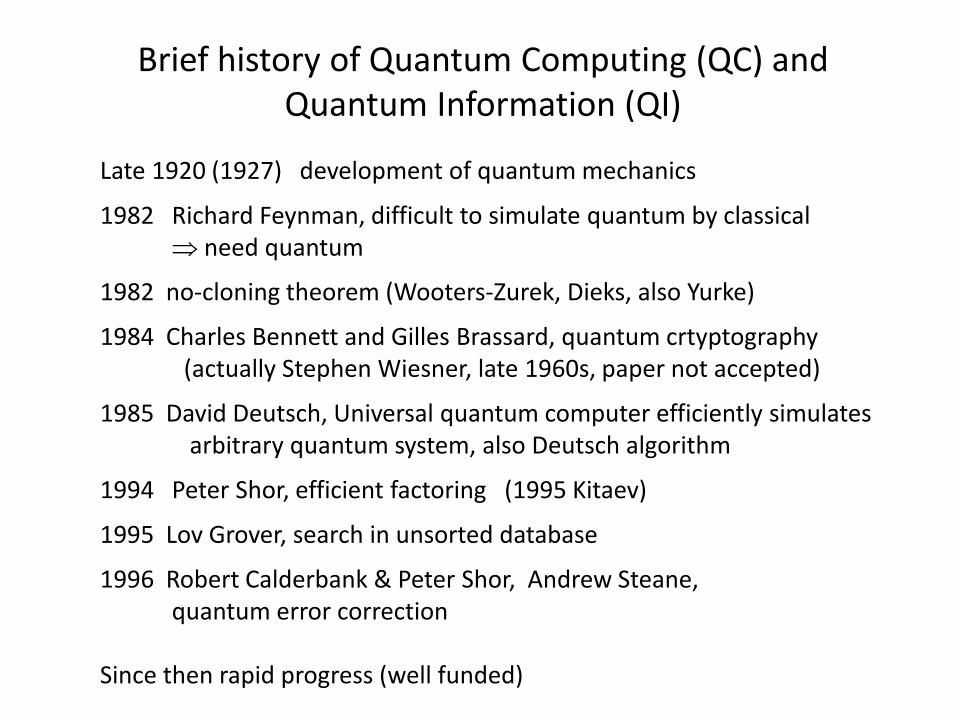
Brief history of Quantum Computing (QC) and Quantum Information (QI)

Late 1920 (1927) development of quantum mechanics

1982 Richard Feynman, difficult to simulate quantum by classical ⇒ need quantum

1982 no-cloning theorem (Wooters-Zurek, Dieks, also Yurke)

1984 Charles Bennett and Gilles Brassard, quantum crtyptography(actually Stephen Wiesner, late 1960s, paper not accepted)

1985 David Deutsch, Universal quantum computer efficiently simulates arbitrary quantum system, also Deutsch algorithm

1994 Peter Shor, efficient factoring (1995 Kitaev)

1995 Lov Grover, search in unsorted database

1996 Robert Calderbank & Peter Shor, Andrew Steane, quantum error correction

Since then rapid progress (well funded)

Structure of the course

Overview of quantum mechanics

General structure of a quantum computer, 1-qubit, 2-qubit, and 3-qubit gates

Usual QC protocol for a function calculation and main trick, toy problems (algorithms)

EPR, Bell states, quantum teleportation, quantum cryptography ----------------------

RSA encryption, Shor’s algorithm for factoring

Grover algorithm

Quantum error correction

Computational complexity (very briefly)

EE214/PHYS220 Quantum Computing

Lecture 2: Quantum mechanics postulates

Postulate 1. State of a quantum system is represented by a vector in a Hilbert space with the norm (“length”) of 1.

Notation: |𝜓𝜓⟩ (“ket-vector”)Hilbert space: complete inner-product space

Linear space, can introduce basis, orthonormal basis

In 1D or 3D case 𝜓𝜓 ↔ 𝜓𝜓(𝑥𝑥) or 𝜓𝜓(𝑟𝑟), so Hilbert space is infinite-dimensional.

In QC much simpler, since Hilbert space is always finite-dimensional.

𝜓𝜓 =

𝛼𝛼0𝛼𝛼1𝛼𝛼2. .. .𝛼𝛼𝑁𝑁

𝜙𝜙 =

𝛽𝛽0𝛽𝛽1𝛽𝛽2. .. .𝛽𝛽𝑁𝑁

𝛼𝛼𝑖𝑖 , 𝛽𝛽𝑖𝑖 are complex numbers

Inner product is

𝜙𝜙 𝜓𝜓 = ∑𝑖𝑖 𝛽𝛽𝑖𝑖∗𝛼𝛼𝑖𝑖

(Dirac notation, bra-ket)

number and order of postulates not important

Different bases are possible (e.g., measurement of spin along different directions)

superposition

“Computational basis”: 000 , 001 , 010 , …

2 qubits, “separable state”

We see that 𝛼𝛼00𝛼𝛼11 = 𝛼𝛼10𝛼𝛼01, while general 2-qubit wavefunction does not satisfy this condition ⇒ most states are not separable (i.e., entangled)

𝜓𝜓 =𝛼𝛼0𝛼𝛼1. .𝛼𝛼7

= 𝛼𝛼0 000 + 𝛼𝛼1 001 + 𝛼𝛼2 010 + ⋯+ 𝛼𝛼7 111

∑𝑖𝑖 𝛼𝛼𝑖𝑖 2 = 1 (normalization)

Most states are entangled: 1 qubit is characterized by 2 complex numbers,so 𝑘𝑘 separate qubits would be characterized by 2𝑘𝑘 complex numbers, but general 𝑘𝑘-qubit state is characterized by 2𝑘𝑘 complex numbers.

𝛼𝛼 0 + 𝛽𝛽 1 ⊗ 𝛾𝛾 0 + 𝛿𝛿|1⟩) = 𝛼𝛼𝛾𝛾 00 + 𝛼𝛼𝛿𝛿 01 + 𝛽𝛽𝛾𝛾 10 + 𝛽𝛽𝛿𝛿 11𝛼𝛼00 𝛼𝛼01 𝛼𝛼10 𝛼𝛼11

Postulate 1 (cont.)

Postulate 2

Properties of Hermitian operators

Hermitian (self-adjoint) operator: �𝐵𝐵† = �𝐵𝐵for a matrix, Hermitian conjugate is 𝐵𝐵𝑖𝑖𝑖𝑖

† = 𝐵𝐵𝑖𝑖𝑖𝑖∗

- Eigenvalues are real - Eigenvectors form orthonormal basis (somewhat oversimplified),

so each observable defines an orthonormal basis, in which its matrix is diagonal (with real elements)

Postulate 2. Measurable quantities (physical magnitudes, dynamical variables,“observables”) are represented by Hermitian operators

Hermitian matrix: 𝐵𝐵𝑖𝑖𝑖𝑖 = 𝐵𝐵𝑖𝑖𝑖𝑖∗ (real on diagonal, complex-conjugate off-diagonal)

Postulate 3

Another way to think:

Postulate 3. Measurement result is necessarily one of eigenvaluesof the corresponding operator (no other results possible).

Measurement result 𝑟𝑟 is generally random, with probability𝑝𝑝𝑟𝑟 = 𝜓𝜓𝑟𝑟 𝜓𝜓 2, where |𝜓𝜓⟩ is the state before measurement

and |𝜓𝜓𝑟𝑟⟩ is the normalized eigenvector, corresponding to the eigenvalue 𝑟𝑟.

If spectrum of the measured operator is degenerate (i.e., a subspace corresponds to the eigenvalue 𝑟𝑟), then we need to choose a basis |𝜓𝜓𝑟𝑟,𝑖𝑖⟩ in this subspace, and

𝑝𝑝𝑟𝑟 = ∑𝑖𝑖 𝜓𝜓𝑟𝑟,𝑖𝑖 𝜓𝜓2

.

𝑝𝑝𝑟𝑟 = �ℙ𝑟𝑟 𝜓𝜓2

where �ℙ𝑟𝑟 is operator of projection onto subspace, corresponding to the eigenvalue 𝑟𝑟and . . denotes norm (“length”) of a vector.

Postulate 3 (cont.)Example

Measure all 3 qubits. 8 possible results.

𝜓𝜓 = 𝛼𝛼0 000 + 𝛼𝛼1 001 + 𝛼𝛼2 010 + ⋯+ 𝛼𝛼7 111

0 ↔ 000 ↔ |000⟩1 ↔ 001 ↔ |001⟩2 ↔ 010 ↔ |010⟩. . .

7 ↔ 111 ↔ |111⟩

𝑃𝑃0 = 𝛼𝛼0 2

𝑃𝑃1 = 𝛼𝛼1 2

𝑃𝑃2 = 𝛼𝛼2 2

. . .𝑃𝑃7 = 𝛼𝛼7 2

Measured observable

�𝑀𝑀 =

01

23

45

67

00 eigenvalue

for corresp.eigenstate(comp.basis)

Now measure only first qubit, results 0 or 1

�𝑀𝑀1 =

00

00

11

11

eigenvectors: 𝛼𝛼0𝛼𝛼1𝛼𝛼2𝛼𝛼30000

for 0

0000𝛼𝛼4𝛼𝛼5𝛼𝛼6𝛼𝛼7

for 1

00

Postulate 3 (cont.)Measure qubits 2 and 3

�𝑀𝑀2 =

00

11

00

11

00

�𝑀𝑀3 =

01

01

01

01

00 �𝑀𝑀 = 4 �𝑀𝑀1 + 2 �𝑀𝑀2 + �𝑀𝑀3

8 eigenvalues: 0, 1, .. 7

Postulate 3’

Postulate 3’. Average (“expectation”) value for measuring operator �𝐵𝐵 is�𝐵𝐵 = 𝜓𝜓 �𝐵𝐵 𝜓𝜓 .

Follows from postulate 3, but often a separate postulate

Important in standard quantum mechanics, but not important for QC(except NMR)

𝜓𝜓 �𝐵𝐵 𝜓𝜓 = 𝛼𝛼0∗ 𝛼𝛼1∗ . .𝛼𝛼𝑁𝑁∗𝑏𝑏00

𝑏𝑏𝑖𝑖𝑖𝑖

𝑏𝑏𝑁𝑁𝑁𝑁

𝛼𝛼0𝛼𝛼1. .𝛼𝛼𝑁𝑁

𝜓𝜓 �𝐵𝐵 𝜓𝜓 = 𝜓𝜓 ( �𝐵𝐵 𝜓𝜓 ) = ( 𝜓𝜓 �𝐵𝐵) 𝜓𝜓Proof

�𝐵𝐵 = ∑𝑟𝑟 𝑟𝑟 �ℙ𝑟𝑟 (since Hermitian)

𝜓𝜓 �𝐵𝐵 𝜓𝜓 = ∑𝑟𝑟 𝑟𝑟 𝜓𝜓 �ℙ𝑟𝑟 𝜓𝜓 = ∑𝑟𝑟 𝑟𝑟 𝜓𝜓 �ℙ𝑟𝑟 �ℙ𝑟𝑟 𝜓𝜓 = ∑𝑟𝑟 𝑟𝑟 �ℙ𝑟𝑟 𝜓𝜓2 = ∑𝑟𝑟 𝑟𝑟 𝑝𝑝𝑟𝑟

QED

Postulate 4

Postulate 4. After measurement of �𝐵𝐵 with result 𝑟𝑟, the state abruptly changes:

(projected onto subspace and normalized)

ExamplesCalled wavefunction collapse

𝜓𝜓 →�ℙ|𝜓𝜓⟩�ℙ 𝜓𝜓

𝜓𝜓 = 𝛼𝛼0 000 + 𝛼𝛼1 001 + 𝛼𝛼2 010 + ⋯+ 𝛼𝛼7 111

(a) Measure all qubits, get result 3 = 011, then 𝜓𝜓 → |011⟩(Does not matter what was before!Cannot get more information on 𝛼𝛼𝑖𝑖.)

(b) Measure only first qubit, get result 0, then

𝜓𝜓 →𝛼𝛼0 000 + 𝛼𝛼1 001 + 𝛼𝛼2 010 + 𝛼𝛼3 011

𝛼𝛼0 2 + 𝛼𝛼1 2 + 𝛼𝛼2 2 + 𝛼𝛼3 2

Postulate 4 (cont.)

Remark

We consider the simplest case: “orthodox” measurement (“projective” measurement); this is essentially common sense

More general: “generalized” measurements (POVM, incomplete, partial,weak, continuous, etc.)

Idea: do not know result exactly, partial information → partial collapse

Techniques of measurement operators (arbitrary linear operator, replacing projectors �ℙ𝑟𝑟), quantum trajectory, Bayesian formalism

Will not use in this course because:- more difficult- generalized measurement can be reduced to orthodox measurement in an extended Hilbert space (indirect meas.)

Postulate 5

Postulate 5. Evolution of a quantum state is described by

the Schrödinger equation ,

where �𝐻𝐻 is the operator of energy (Hamiltonian)

𝑑𝑑|𝜓𝜓⟩𝑑𝑑𝑑𝑑 = −

𝑖𝑖ℏ�𝐻𝐻|𝜓𝜓⟩

We will not really use it, but important that evolution is described by a unitary operator

𝜓𝜓 𝑑𝑑 = 𝑒𝑒−𝑖𝑖ℏ�𝐻𝐻𝑡𝑡 𝜓𝜓 0 = �𝑈𝑈 |𝜓𝜓 0 ⟩

Since �𝐻𝐻 is Hermitian, �𝑈𝑈 is unitary, �𝑈𝑈† = �𝑈𝑈−1 �𝑈𝑈�𝑈𝑈† = �𝑈𝑈† �𝑈𝑈 = �1

A unitary operator preserves inner product

�𝑈𝑈𝜙𝜙 �𝑈𝑈𝜓𝜓 = 𝜙𝜙 �𝑈𝑈† �𝑈𝑈𝜓𝜓⟩ = ⟨𝜙𝜙|𝜓𝜓⟩

Unitary operator transforms an orthonormal basis into an orthonormal basis (rotation of a space)

Quantum computer operation

Evolution in a quantum computer (quantum gates) is described by unitary operators

Can be only one measurement at the very end, but for error correction should also be many measurement steps during operation

A quantum computer consists of unitary gates (usually one-qubit and two-qubit gates) and measurement stages