Summer 2010 Draft 3 EECS 149

UC Berkeley EECS 1

EE149: NaturalPoint Tracking Tools

Dorsa Sadigh Philip Weiss

July 20, 2010 1. Background: OptiTrack is a motion capture system made by NaturalPoint Inc. It has been on the market since 2005, and competes with Phase Space motion capture system. OptiTrack provides premium optical motion capture, and tracking solutions for commercial, industrial, game development and research. The software toolkits are designed for rigid body tracking, full body motion capture and face motion capture. The EECS 149 lab is equipped with five-camera system capable of tracking iRobots with high-speed grayscale video at 100 fps. The toolkit used for localization of robots is “Tracking Tools” provided by NaturalPoint. The position and orientation data of iRobots streamed from the optitrack cameras can be saved in CSV format or sent over network in real-time. 2. Tracking Tools Setup:

NaturalPoint Tracking Tools Application provides calibration and real-time 3D optical tracking of multiple rigid bodies tracking across multiple OptiTrack cameras. In this document, you are provided with the basics of starting Tracking Tools Application, Calibration and Streaming OptiTrack data. This document should be used after complete installation of software and hardware. Much of the material from this document is taken from [1-3] and reproduced with permission.

2.1 Rigid Bodies and Markers: NaturalPoint provides different types of spherical reflective markers. These markers can be tracked in 3DOF (X, Y, Z) physical coordinates using Tracking Tools software.

Fig.1. Spherical Markers

Summer 2010 Draft 3 EECS 149

UC Berkeley EECS 2

Besides the markers, other reflective material such as reflective dots, and reflective strip are provided by NaturalPoint that can be attached to the trackable objects.

Fig.2. Reflective Material

In order to track an object in 3 dimensions using Tracking Tools software, you must define a rigid body with minimum number of three markers. It is recommended to use the spherical reflective markers instead of hemispheric and flat markers since their shape as it appears to the camera may change when they rotate, and this can introduce errors when calculating center of mass and position of rigid body.

Using more than three markers can increase precision, and reduce the likelihood of the rigid body flipping; however, it might also create redundancy.

The markers defining a rigid body shouldn’t be too close to each other; markers closer than 6 mm can cause incorrect 3D position data, and if the calibration is poor the rays from the markers might be grouped incorrectly and result in false orientation, or misidentified marker location.

It is recommended to arrange markers in asymmetrical patterns as it improves reliability. Also while defining multiple rigid bodies make sure to use unique arrangements of markers to avoid misidentification or swapping.

A rigid body can be created by selecting the markers we want to include, and right clicking on the selection: Trackables → Create Trackable (as shown in Figure 3). After creating one/multiple rigid bodies, the software is ready to track them in full 6DOF (position and orientation).

Summer 2010 Draft 3 EECS 149

UC Berkeley EECS 3

Fig.3. Creating a Trackable Object

All the other parameters of rigid bodies can be set by using Trackables pane__ the right window shown in Figure 3. These parameters allow the user to choose how flexible the Tracking Tools solver is. A number of these parameters are: Dynamic/ Static Constraints, Smoothing Settings, and Maximum Marker Deflection.

2.2. Calibration:

There are two methods of Calibration provided by the NaturalPoint Tracking Tools. One Marker Calibration is the original method; however, NaturalPoint has provided a newer calibration algorithm since March 2010, which is the Three Marker Calibration. In order to utilize this method, a three-marker wand is required. NaturalPoint provides its own three-marker optiwand for this method of calibration.

Fig.4. Optiwand In order to start the Calibration, start the Tracking Tools Application, and choose “Perform Camera Calibration” from the “Tracking Tools Quick Start” window. You can always start a camera calibration from the Layout menu → Camera Calibration

Summer 2010 Draft 3 EECS 149

UC Berkeley EECS 4

Fig.5. Start up menu

Before Starting the Calibration, there are a few things that must be checked for achieving the best calibration:

1. Prepare the Capture Volume a. Remove extraneous markers from the volume. b. Remove reflective objects from the trackable.

2. Adjust Camera Settings: a. Block remaining visible reflective objects. b. Block camera’s infrared reflection on the floor. This reflection might be thought as a

reflective marker if not blocked. (See the image of this reflection in Figure 13). c. Adjust camera settings.

3. Make sure you have chosen the correct lens type on the 3-Marker Calibration setting. You can check this at: 3-Marker Calibration pane → Calibration → Solver Options → Lens Type. The default for this setting is 4.5mm; however, in the EE149 lab we are using R2 cameras with lens type 57.5º FOV (3.5mm). So change the setting to 3.5mm(wide).

All the visible markers must be blocked at this point by using “Block Visible” option from “Camera Group Properties” pane. Then click on the “Start Wanding” button from the “3-Marker Calibration” window, and start wanding. Wanding must be done evenly and comprehensively through the entire capture volume, while ensuring the best possible coverage for each 2D camera view.

Summer 2010 Draft 3 EECS 149

UC Berkeley EECS 5

Fig.6. Wanding to Collect Data for Calibration

While wanding the calibration engine (on the bottom right of Figure 6) shows the number of samples for each camera, as well as a measure of the 3D distribution of those sample points. A better view of this information is shown in Figure 9.

When enough data is collected the background of the calibration engine turns green, and it displays “Sufficient for Quality: Very High”.

After collecting enough data for a desired quality, you can press the “calculate” button. The 3-Marker calculation is divided into three phases: 1. An initial solution estimation, 2. An initial error minimization, 3. Final global optimization. During the solving process, the calibration will take the initial estimated solution, and minimize the 3D triangulation error by globally optimizing both the camera’s extrinsic position and orientation as well as its intrinsic focal and lens distortion characteristics.

When the solution has reached an acceptable quality it will signify the user that it is “Ready to Apply” (shown in Figure 8).

Summer 2010 Draft 3 EECS 149

UC Berkeley EECS 6

Fig.7. Calculation of Data for Global Optimization

Fig.8.Calculation Fig.9.Wanding

When the user clicks on “Apply Result”, Tracking Tools software presents a calibration report with the overall calibration result that is shown at the top. The user can choose between two options either “Apply”, or “Apply and Refine”. When the desired result is achieved, the user can apply the result.

At this point, the user may want to save the calibration, and the original wanding data for later use. The next step is to set the ground plane. Put the ground plane at the origin, and under 3-Marker Calibration → Ground Plane click on “Set Ground Plane”.

Summer 2010 Draft 3 EECS 149

UC Berkeley EECS 7

Now the volume is calibrated and the user can track objects.

Fig.10. Ground Plane 3. Real-Time Tracking: Tracking Tools user has two options for using the rigid bodies data. One is exporting data using files, and the more interesting one is streaming data in real-time. 3.1. Exporting to CSV format: Tracking data can be recorded using “Record and Playback” pane. After recording data, you can go to File → Export Tracking Data… This exports the data in the CSV (Comma-Separated Values) format, and the user can have access to data using Microsoft Excel. The format data comes through is starting with a header at the top being followed by all the tracking information. 3.2. Streaming Tracking Data: Tracking Tools software provides three industry standard streaming protocols. In order to use any of these protocols, you must open the “Streaming Properties” pane, and choose one of the following three streaming options. All of these streaming methods are built on network transport, and is streamed over TCP/IP. 3.2.1. Natural Point Engine (NatNet): This streaming engine is a custom streaming engine provided by NaturalPoint. The important point about this method is that it streams markers’ coordinates as well as the rigid bodies’ position and orientation. Streams: rigid bodies, and markers. Network Details: port 1510, multicast group 1001, UDP multicast 3.2.2. Trackd Engine: Streams: rigid bodies Network Detail: port 4994, TCP + UDP 3.2.3. VRPN Engine: VRPN Streaming is the method that we have used to localize iRobots. It is also the method recommended by NaturalPoint. It features low latency and has built-in auto-renegotiation if a connection is temporarily dropped. In order to use vrpn engine, the vrpn library needs to be included in the source code.

Summer 2010 Draft 3 EECS 149

UC Berkeley EECS 8

Streams: rigid bodies Network Details: selectable port, default port 3883, TCP + UDP

4. A Quick Start on iRobot Localization: At this stage, we are ready to track iRobots. Attach three spherical markers to the iRobot (as shown in Figure 11), and place the iRobot in capture volume.

Fig.11. iRobot with 3 Reflective Markers

Open the Tracking Tools Application, and Perform Camera Calibration, or open a saved calibration by using Open Camera Calibration option. You should be able to see the iRobot with three markers in the capture volume. Figure 12 is a view of what the tracking tools software displays at this point. The cameras can also be set in the grayscale mode as shown in Figure 13.

Summer 2010 Draft 3 EECS 149

UC Berkeley EECS 9

Fig.12. iRobot Found as a Rigid Body

Fig.13. iRobot found by 5 Cameras: Camera 1 and 2 in GrayScale mode.

Summer 2010 Draft 3 EECS 149

UC Berkeley EECS 10

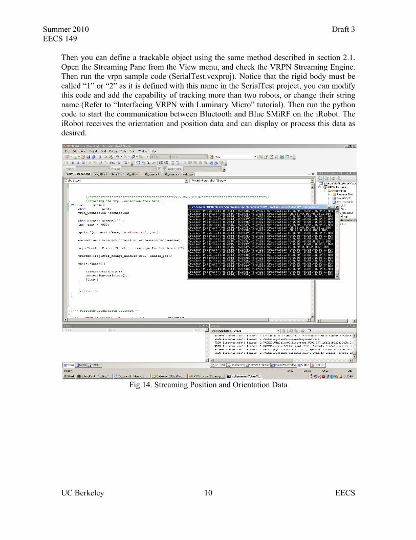
Then you can define a trackable object using the same method described in section 2.1. Open the Streaming Pane from the View menu, and check the VRPN Streaming Engine. Then run the vrpn sample code (SerialTest.vcxproj). Notice that the rigid body must be called “1” or “2” as it is defined with this name in the SerialTest project, you can modify this code and add the capability of tracking more than two robots, or change their string name (Refer to “Interfacing VRPN with Luminary Micro” tutorial). Then run the python code to start the communication between Bluetooth and Blue SMiRF on the iRobot. The iRobot receives the orientation and position data and can display or process this data as desired.

Fig.14. Streaming Position and Orientation Data

Summer 2010 Draft 3 EECS 149

UC Berkeley EECS 11

References:

1. NaturalPoint Tracking Tools Manual: http://www.naturalpoint.com/optitrack/support/manuals/

2. NaturalPoint Tracking Tools Training and Tutorial Series: http://www.naturalpoint.com/optitrack/products/tracking-tools/videos.html

3. NaturalPoint ARENA 3-Marker Calibration: http://www.naturalpoint.com/optitrack/products/camera-calibration.html