EE101: Digital circuits (Part 1) - Department of
144
EE101: Digital circuits (Part 1) M. B. Patil [email protected] www.ee.iitb.ac.in/~sequel Department of Electrical Engineering Indian Institute of Technology Bombay M. B. Patil, IIT Bombay
Transcript of EE101: Digital circuits (Part 1) - Department of

EE101: Digital circuits (Part 1)
M. B. [email protected]
www.ee.iitb.ac.in/~sequel
Department of Electrical EngineeringIndian Institute of Technology Bombay
M. B. Patil, IIT Bombay

Digital circuits
t t
analog signal digital signal
0
1high
low
* For an analog signal x(t), the actual value (a real number) at a given time isimportant.
* A digital signal, on the other hand, is “binary” in nature, i.e., it takes on onlytwo values: low (0) or high (1).
* Although we have shown 0 and 1 as constant levels, in reality, that is notrequired. Any value in the low (high) band will be interpreted as 0 (1) by digitalcircuits.
* The definition of low and high bands depends on the technology used, such asTTL (Transitor-Transitor Logic), CMOS (Complementary MOS), ECL(Emitter-Coupled Logic), etc.
M. B. Patil, IIT Bombay
A simple digital circuit
E
B
C
0 1 2 3 4 5
1
2
3
4
5
0
Vi
RC
VCC
Vo
RB Vo(Volts)
Vi (Volts)
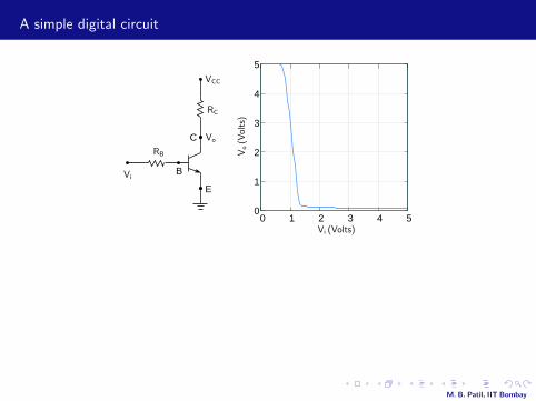
* If Vi is low (“0”), Vo is high (“1”).If Vi is high (“1”), Vo is low (“0”).
* The circuit is called an “inverter” because it inverts the logic level of the input.If the input is 0, it makes the output 1, and vice versa.
* Digital circuits are made using a variety of devices. The simple BJT inverter wehave shown should only be considered as an illustrative circuit.
* Most of the VLSI circuits today employ the MOS technology because of the highpacking density and low power consumption it offers.
M. B. Patil, IIT Bombay

A simple digital circuit
E
B
C
0 1 2 3 4 5
1
2
3
4
5
0
Vi
RC
VCC
Vo
RB Vo(Volts)
Vi (Volts)
* If Vi is low (“0”), Vo is high (“1”).If Vi is high (“1”), Vo is low (“0”).
* The circuit is called an “inverter” because it inverts the logic level of the input.If the input is 0, it makes the output 1, and vice versa.
* Digital circuits are made using a variety of devices. The simple BJT inverter wehave shown should only be considered as an illustrative circuit.
* Most of the VLSI circuits today employ the MOS technology because of the highpacking density and low power consumption it offers.
M. B. Patil, IIT Bombay

Digital circuits
original data corrupted data recovered data
comparatort t t
V3
Vref
V2
V1 V2
Vref
V3
* A major advantage of digital systems is that, even if the original data getsdistorted (e.g., in transmitting through optical fibre or storing on a CD) due tonoise, attenuation, etc., it can be retrieved easily.
* There are several other benefits of using digital representation:
- can use computers to process the data.- can store in a variety of storage media.
- can program the functionality. For example, the behaviour of a digital filter
can be changed simply by changing its coefficients.
M. B. Patil, IIT Bombay

Digital circuits
original data corrupted data recovered data
comparatort t t
V3
Vref
V2
V1 V2
Vref
V3
* A major advantage of digital systems is that, even if the original data getsdistorted (e.g., in transmitting through optical fibre or storing on a CD) due tonoise, attenuation, etc., it can be retrieved easily.
* There are several other benefits of using digital representation:
- can use computers to process the data.
- can store in a variety of storage media.
- can program the functionality. For example, the behaviour of a digital filter
can be changed simply by changing its coefficients.
M. B. Patil, IIT Bombay

Digital circuits
original data corrupted data recovered data
comparatort t t
V3
Vref
V2
V1 V2
Vref
V3
* A major advantage of digital systems is that, even if the original data getsdistorted (e.g., in transmitting through optical fibre or storing on a CD) due tonoise, attenuation, etc., it can be retrieved easily.
* There are several other benefits of using digital representation:
- can use computers to process the data.- can store in a variety of storage media.
- can program the functionality. For example, the behaviour of a digital filter
can be changed simply by changing its coefficients.
M. B. Patil, IIT Bombay

Digital circuits
original data corrupted data recovered data
comparatort t t
V3
Vref
V2
V1 V2
Vref
V3
* A major advantage of digital systems is that, even if the original data getsdistorted (e.g., in transmitting through optical fibre or storing on a CD) due tonoise, attenuation, etc., it can be retrieved easily.
* There are several other benefits of using digital representation:
- can use computers to process the data.- can store in a variety of storage media.
- can program the functionality. For example, the behaviour of a digital filter
can be changed simply by changing its coefficients.
M. B. Patil, IIT Bombay
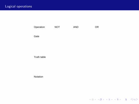
Logical operations
Gate
Truth table
Notation
Operation NOT AND OR
10
01
YA
Y = A
A Y
1
1
1 1 1
0 0 0
0
0 0
0
A B Y
= AB
Y = A · B
B
AY
1
1
1 1 1
0 0 0
0
0
A B Y
1
1
Y = A+ B
A
BY
M. B. Patil, IIT Bombay

Logical operations
Gate
Truth table
Notation
Operation NOT AND OR
10
01
YA
Y = A
A Y
1
1
1 1 1
0 0 0
0
0 0
0
A B Y
= AB
Y = A · B
B
AY
1
1
1 1 1
0 0 0
0
0
A B Y
1
1
Y = A+ B
A
BY
M. B. Patil, IIT Bombay

Logical operations
Gate
Truth table
Notation
Operation NOT AND OR
10
01
YA
Y = A
A Y
1
1
1 1 1
0 0 0
0
0 0
0
A B Y
= AB
Y = A · B
B
AY
1
1
1 1 1
0 0 0
0
0
A B Y
1
1
Y = A+ B
A
BY
M. B. Patil, IIT Bombay

Logical operations
Gate
Truth table
Notation
Operation NOT AND OR
10
01
YA
Y = A
A Y
1
1
1 1 1
0 0 0
0
0 0
0
A B Y
= AB
Y = A · B
B
AY
1
1
1 1 1
0 0 0
0
0
A B Y
1
1
Y = A+ B
A
BY
M. B. Patil, IIT Bombay

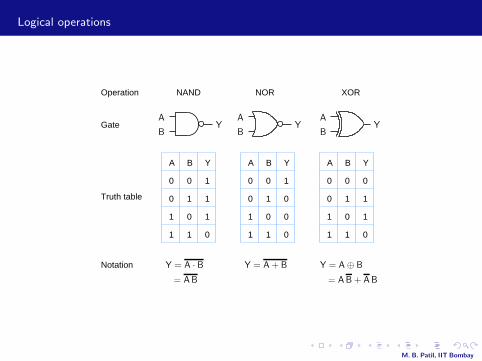
Logical operations
Gate
Truth table
Notation
Operation NORNAND XOR
1
1
1 1
0 0
0
0
A B Y
1
1
1
0
Y = A · B= AB
YA
B
1
1
1 1
0 0
0
0 0
0
A B Y
1
0
Y = A+ B
B
AY
1
1
1 1
0 0 0
0
0
A B Y
1
1
0
Y = A⊕ B
= AB+ AB
A
BY
M. B. Patil, IIT Bombay

Logical operations
Gate
Truth table
Notation
Operation NORNAND XOR
1
1
1 1
0 0
0
0
A B Y
1
1
1
0
Y = A · B= AB
YA
B
1
1
1 1
0 0
0
0 0
0
A B Y
1
0
Y = A+ B
B
AY
1
1
1 1
0 0 0
0
0
A B Y
1
1
0
Y = A⊕ B
= AB+ AB
A
BY
M. B. Patil, IIT Bombay

Logical operations
Gate
Truth table
Notation
Operation NORNAND XOR
1
1
1 1
0 0
0
0
A B Y
1
1
1
0
Y = A · B= AB
YA
B
1
1
1 1
0 0
0
0 0
0
A B Y
1
0
Y = A+ B
B
AY
1
1
1 1
0 0 0
0
0
A B Y
1
1
0
Y = A⊕ B
= AB+ AB
A
BY
M. B. Patil, IIT Bombay
Logical operations
Gate
Truth table
Notation
Operation NORNAND XOR
1
1
1 1
0 0
0
0
A B Y
1
1
1
0
Y = A · B= AB
YA
B
1
1
1 1
0 0
0
0 0
0
A B Y
1
0
Y = A+ B
B
AY
1
1
1 1
0 0 0
0
0
A B Y
1
1
0
Y = A⊕ B
= AB+ AB
A
BY
M. B. Patil, IIT Bombay

Logical operations
* The AND operation is commutative.
→ A · B = B · A.
* The AND operation is associative.
→ (A · B) · C = A · (B · C).
* The OR operation is commutative.
→ A + B = B + A.
* The OR operation is associative.
→ (A + B) + C = A + (B + C).
M. B. Patil, IIT Bombay

Logical operations
* The AND operation is commutative.
→ A · B = B · A.
* The AND operation is associative.
→ (A · B) · C = A · (B · C).
* The OR operation is commutative.
→ A + B = B + A.
* The OR operation is associative.
→ (A + B) + C = A + (B + C).
M. B. Patil, IIT Bombay

Logical operations
* The AND operation is commutative.
→ A · B = B · A.
* The AND operation is associative.
→ (A · B) · C = A · (B · C).
* The OR operation is commutative.
→ A + B = B + A.
* The OR operation is associative.
→ (A + B) + C = A + (B + C).
M. B. Patil, IIT Bombay

Logical operations
* The AND operation is commutative.
→ A · B = B · A.
* The AND operation is associative.
→ (A · B) · C = A · (B · C).
* The OR operation is commutative.
→ A + B = B + A.
* The OR operation is associative.
→ (A + B) + C = A + (B + C).
M. B. Patil, IIT Bombay

Boolean algebra (George Boole, 1815-1864)
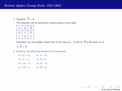
* Theorem: A = A.
The theorem can be proved by constructing a truth table:
A A A
0 1 0
1 0 1
Therefore, for all possible values that A can take (i.e., 0 and 1), A is the same as A.
⇒ A = A.
* Similarly, the following theorems can be proved:
A + 0 = A A · 1 = A
A + 1 = 1 A · 0 = 0
A + A = A A · A = A
A + A = 1 A · A = 0
Note the duality: (+↔ ·) and (1↔ 0).
M. B. Patil, IIT Bombay

Boolean algebra (George Boole, 1815-1864)
* Theorem: A = A.
The theorem can be proved by constructing a truth table:
A A A
0 1 0
1 0 1
Therefore, for all possible values that A can take (i.e., 0 and 1), A is the same as A.
⇒ A = A.
* Similarly, the following theorems can be proved:
A + 0 = A A · 1 = A
A + 1 = 1 A · 0 = 0
A + A = A A · A = A
A + A = 1 A · A = 0
Note the duality: (+↔ ·) and (1↔ 0).
M. B. Patil, IIT Bombay

De Morgan’s theorems
A B A + B A + B A B A · B A · B A · B A + B
0 0
0 1 1 1 1 0 1 1
0 1
1 0 1 0 0 0 1 1
1 0
1 0 0 1 0 0 1 1
1 1
1 0 0 0 0 1 0 0
* Comparing the truth tables for A + B and AB, we conclude that A + B = AB.
* Similiarly, A · B = A + B.
* Similar relations hold for more than two variables, e.g.,
A · B · C = A + B + C ,
A + B + C + D = A · B · C · D,
(A + B) · C = (A + B) + C .
M. B. Patil, IIT Bombay

De Morgan’s theorems
A B A + B A + B A B A · B A · B A · B A + B
0 0 0
1 1 1 1 0 1 1
0 1 1
0 1 0 0 0 1 1
1 0 1
0 0 1 0 0 1 1
1 1 1
0 0 0 0 1 0 0
* Comparing the truth tables for A + B and AB, we conclude that A + B = AB.
* Similiarly, A · B = A + B.
* Similar relations hold for more than two variables, e.g.,
A · B · C = A + B + C ,
A + B + C + D = A · B · C · D,
(A + B) · C = (A + B) + C .
M. B. Patil, IIT Bombay

De Morgan’s theorems
A B A + B A + B A B A · B A · B A · B A + B
0 0 0 1
1 1 1 0 1 1
0 1 1 0
1 0 0 0 1 1
1 0 1 0
0 1 0 0 1 1
1 1 1 0
0 0 0 1 0 0
* Comparing the truth tables for A + B and AB, we conclude that A + B = AB.
* Similiarly, A · B = A + B.
* Similar relations hold for more than two variables, e.g.,
A · B · C = A + B + C ,
A + B + C + D = A · B · C · D,
(A + B) · C = (A + B) + C .
M. B. Patil, IIT Bombay

De Morgan’s theorems
A B A + B A + B A B A · B A · B A · B A + B
0 0 0 1 1
1 1 0 1 1
0 1 1 0 1
0 0 0 1 1
1 0 1 0 0
1 0 0 1 1
1 1 1 0 0
0 0 1 0 0
* Comparing the truth tables for A + B and AB, we conclude that A + B = AB.
* Similiarly, A · B = A + B.
* Similar relations hold for more than two variables, e.g.,
A · B · C = A + B + C ,
A + B + C + D = A · B · C · D,
(A + B) · C = (A + B) + C .
M. B. Patil, IIT Bombay

De Morgan’s theorems
A B A + B A + B A B A · B A · B A · B A + B
0 0 0 1 1 1
1 0 1 1
0 1 1 0 1 0
0 0 1 1
1 0 1 0 0 1
0 0 1 1
1 1 1 0 0 0
0 1 0 0
* Comparing the truth tables for A + B and AB, we conclude that A + B = AB.
* Similiarly, A · B = A + B.
* Similar relations hold for more than two variables, e.g.,
A · B · C = A + B + C ,
A + B + C + D = A · B · C · D,
(A + B) · C = (A + B) + C .
M. B. Patil, IIT Bombay

De Morgan’s theorems
A B A + B A + B A B A · B A · B A · B A + B
0 0 0 1 1 1 1
0 1 1
0 1 1 0 1 0 0
0 1 1
1 0 1 0 0 1 0
0 1 1
1 1 1 0 0 0 0
1 0 0
* Comparing the truth tables for A + B and AB, we conclude that A + B = AB.
* Similiarly, A · B = A + B.
* Similar relations hold for more than two variables, e.g.,
A · B · C = A + B + C ,
A + B + C + D = A · B · C · D,
(A + B) · C = (A + B) + C .
M. B. Patil, IIT Bombay

De Morgan’s theorems
A B A + B A + B A B A · B A · B A · B A + B
0 0 0 1 1 1 1 0
1 1
0 1 1 0 1 0 0 0
1 1
1 0 1 0 0 1 0 0
1 1
1 1 1 0 0 0 0 1
0 0
* Comparing the truth tables for A + B and AB, we conclude that A + B = AB.
* Similiarly, A · B = A + B.
* Similar relations hold for more than two variables, e.g.,
A · B · C = A + B + C ,
A + B + C + D = A · B · C · D,
(A + B) · C = (A + B) + C .
M. B. Patil, IIT Bombay

De Morgan’s theorems
A B A + B A + B A B A · B A · B A · B A + B
0 0 0 1 1 1 1 0 1
1
0 1 1 0 1 0 0 0 1
1
1 0 1 0 0 1 0 0 1
1
1 1 1 0 0 0 0 1 0
0
* Comparing the truth tables for A + B and AB, we conclude that A + B = AB.
* Similiarly, A · B = A + B.
* Similar relations hold for more than two variables, e.g.,
A · B · C = A + B + C ,
A + B + C + D = A · B · C · D,
(A + B) · C = (A + B) + C .
M. B. Patil, IIT Bombay

De Morgan’s theorems
A B A + B A + B A B A · B A · B A · B A + B
0 0 0 1 1 1 1 0 1 1
0 1 1 0 1 0 0 0 1 1
1 0 1 0 0 1 0 0 1 1
1 1 1 0 0 0 0 1 0 0
* Comparing the truth tables for A + B and AB, we conclude that A + B = AB.
* Similiarly, A · B = A + B.
* Similar relations hold for more than two variables, e.g.,
A · B · C = A + B + C ,
A + B + C + D = A · B · C · D,
(A + B) · C = (A + B) + C .
M. B. Patil, IIT Bombay

Distributive laws
1. A · (B + C) = AB + AC .
A B C B + C A · (B + C) AB AC AB + AC
0 0 0
0 0 0 0 0
0 0 1
1 0 0 0 0
0 1 0
1 0 0 0 0
0 1 1
1 0 0 0 0
1 0 0
0 0 0 0 0
1 0 1
1 1 0 1 1
1 1 0
1 1 1 0 1
1 1 1
1 1 1 1 1
↑ ↑
M. B. Patil, IIT Bombay

Distributive laws
1. A · (B + C) = AB + AC .
A B C B + C A · (B + C) AB AC AB + AC
0 0 0
0 0 0 0 0
0 0 1
1 0 0 0 0
0 1 0
1 0 0 0 0
0 1 1
1 0 0 0 0
1 0 0
0 0 0 0 0
1 0 1
1 1 0 1 1
1 1 0
1 1 1 0 1
1 1 1
1 1 1 1 1
↑ ↑
M. B. Patil, IIT Bombay

Distributive laws
1. A · (B + C) = AB + AC .
A B C B + C A · (B + C) AB AC AB + AC
0 0 0 0
0 0 0 0
0 0 1 1
0 0 0 0
0 1 0 1
0 0 0 0
0 1 1 1
0 0 0 0
1 0 0 0
0 0 0 0
1 0 1 1
1 0 1 1
1 1 0 1
1 1 0 1
1 1 1 1
1 1 1 1
↑ ↑
M. B. Patil, IIT Bombay

Distributive laws
1. A · (B + C) = AB + AC .
A B C B + C A · (B + C) AB AC AB + AC
0 0 0 0 0
0 0 0
0 0 1 1 0
0 0 0
0 1 0 1 0
0 0 0
0 1 1 1 0
0 0 0
1 0 0 0 0
0 0 0
1 0 1 1 1
0 1 1
1 1 0 1 1
1 0 1
1 1 1 1 1
1 1 1
↑ ↑
M. B. Patil, IIT Bombay

Distributive laws
1. A · (B + C) = AB + AC .
A B C B + C A · (B + C) AB AC AB + AC
0 0 0 0 0 0
0 0
0 0 1 1 0 0
0 0
0 1 0 1 0 0
0 0
0 1 1 1 0 0
0 0
1 0 0 0 0 0
0 0
1 0 1 1 1 0
1 1
1 1 0 1 1 1
0 1
1 1 1 1 1 1
1 1
↑ ↑
M. B. Patil, IIT Bombay

Distributive laws
1. A · (B + C) = AB + AC .
A B C B + C A · (B + C) AB AC AB + AC
0 0 0 0 0 0 0
0
0 0 1 1 0 0 0
0
0 1 0 1 0 0 0
0
0 1 1 1 0 0 0
0
1 0 0 0 0 0 0
0
1 0 1 1 1 0 1
1
1 1 0 1 1 1 0
1
1 1 1 1 1 1 1
1
↑ ↑
M. B. Patil, IIT Bombay

Distributive laws
1. A · (B + C) = AB + AC .
A B C B + C A · (B + C) AB AC AB + AC
0 0 0 0 0 0 0 0
0 0 1 1 0 0 0 0
0 1 0 1 0 0 0 0
0 1 1 1 0 0 0 0
1 0 0 0 0 0 0 0
1 0 1 1 1 0 1 1
1 1 0 1 1 1 0 1
1 1 1 1 1 1 1 1
↑ ↑
M. B. Patil, IIT Bombay

Distributive laws
1. A · (B + C) = AB + AC .
A B C B + C A · (B + C) AB AC AB + AC
0 0 0 0 0 0 0 0
0 0 1 1 0 0 0 0
0 1 0 1 0 0 0 0
0 1 1 1 0 0 0 0
1 0 0 0 0 0 0 0
1 0 1 1 1 0 1 1
1 1 0 1 1 1 0 1
1 1 1 1 1 1 1 1
↑ ↑
M. B. Patil, IIT Bombay

Distributive laws
2. A + B · C = (A + B) · (A + C).
A B C B C A + B C A + B A + C (A + B) (A + C)
0 0 0
0 0 0 0 0
0 0 1
0 0 0 1 0
0 1 0
0 0 1 0 0
0 1 1
1 1 1 1 1
1 0 0
0 1 1 1 1
1 0 1
0 1 1 1 1
1 1 0
0 1 1 1 1
1 1 1
1 1 1 1 1
↑ ↑
M. B. Patil, IIT Bombay

Distributive laws
2. A + B · C = (A + B) · (A + C).
A B C B C A + B C A + B A + C (A + B) (A + C)
0 0 0
0 0 0 0 0
0 0 1
0 0 0 1 0
0 1 0
0 0 1 0 0
0 1 1
1 1 1 1 1
1 0 0
0 1 1 1 1
1 0 1
0 1 1 1 1
1 1 0
0 1 1 1 1
1 1 1
1 1 1 1 1
↑ ↑
M. B. Patil, IIT Bombay

Distributive laws
2. A + B · C = (A + B) · (A + C).
A B C B C A + B C A + B A + C (A + B) (A + C)
0 0 0 0
0 0 0 0
0 0 1 0
0 0 1 0
0 1 0 0
0 1 0 0
0 1 1 1
1 1 1 1
1 0 0 0
1 1 1 1
1 0 1 0
1 1 1 1
1 1 0 0
1 1 1 1
1 1 1 1
1 1 1 1
↑ ↑
M. B. Patil, IIT Bombay

Distributive laws
2. A + B · C = (A + B) · (A + C).
A B C B C A + B C A + B A + C (A + B) (A + C)
0 0 0 0 0
0 0 0
0 0 1 0 0
0 1 0
0 1 0 0 0
1 0 0
0 1 1 1 1
1 1 1
1 0 0 0 1
1 1 1
1 0 1 0 1
1 1 1
1 1 0 0 1
1 1 1
1 1 1 1 1
1 1 1
↑ ↑
M. B. Patil, IIT Bombay

Distributive laws
2. A + B · C = (A + B) · (A + C).
A B C B C A + B C A + B A + C (A + B) (A + C)
0 0 0 0 0 0
0 0
0 0 1 0 0 0
1 0
0 1 0 0 0 1
0 0
0 1 1 1 1 1
1 1
1 0 0 0 1 1
1 1
1 0 1 0 1 1
1 1
1 1 0 0 1 1
1 1
1 1 1 1 1 1
1 1
↑ ↑
M. B. Patil, IIT Bombay

Distributive laws
2. A + B · C = (A + B) · (A + C).
A B C B C A + B C A + B A + C (A + B) (A + C)
0 0 0 0 0 0 0
0
0 0 1 0 0 0 1
0
0 1 0 0 0 1 0
0
0 1 1 1 1 1 1
1
1 0 0 0 1 1 1
1
1 0 1 0 1 1 1
1
1 1 0 0 1 1 1
1
1 1 1 1 1 1 1
1
↑ ↑
M. B. Patil, IIT Bombay

Distributive laws
2. A + B · C = (A + B) · (A + C).
A B C B C A + B C A + B A + C (A + B) (A + C)
0 0 0 0 0 0 0 0
0 0 1 0 0 0 1 0
0 1 0 0 0 1 0 0
0 1 1 1 1 1 1 1
1 0 0 0 1 1 1 1
1 0 1 0 1 1 1 1
1 1 0 0 1 1 1 1
1 1 1 1 1 1 1 1
↑ ↑
M. B. Patil, IIT Bombay

Distributive laws
2. A + B · C = (A + B) · (A + C).
A B C B C A + B C A + B A + C (A + B) (A + C)
0 0 0 0 0 0 0 0
0 0 1 0 0 0 1 0
0 1 0 0 0 1 0 0
0 1 1 1 1 1 1 1
1 0 0 0 1 1 1 1
1 0 1 0 1 1 1 1
1 1 0 0 1 1 1 1
1 1 1 1 1 1 1 1
↑ ↑
M. B. Patil, IIT Bombay

Useful theorems
* A + AB = A.To prove this theorem, we can follow two approaches:
(a) Construct truth tables for LHS and RHS for all possible inputcombinations, and show that they are the same.
(b) Use identities and theorems stated earlier to show that LHS=RHS.
A + AB = A · 1 + A · B= A · (1 + B)= A · (1)= A
* A · (A + B) = A.
Proof: A · (A + B) = A · A + A · B= A + AB= A
M. B. Patil, IIT Bombay

Duality
A + AB = A ←→ A · (A + B) = A.
Note the duality between OR and AND.
Dual of A + AB (LHS): AB → A + BA + AB → A · (A + B).
Dual of A (RHS) = A (since there are no operations ivolved).
⇒ A · (A + B) = A.
Similarly, consider A + A = 1, with (+↔ .) and (1↔ 0).
Dual of LHS = A · A.
Dual of RHS = 0.
⇒ A · A = 0.
M. B. Patil, IIT Bombay

Useful theorems
* A + AB = A + B.
Proof: A + AB = (A + A) · (A + B) (by distributive law)
= 1 · (A + B)
= A + B
Dual theorem: A · (A + B) = AB.
* AB + AB = A.
Proof: AB + AB = A · (B + B) (by distributive law)
= A · 1= A
Dual theorem: (A + B) · (A + B) = A.
M. B. Patil, IIT Bombay

Useful theorems
* A + AB = A + B.
Proof: A + AB = (A + A) · (A + B) (by distributive law)
= 1 · (A + B)
= A + B
Dual theorem: A · (A + B) = AB.
* AB + AB = A.
Proof: AB + AB = A · (B + B) (by distributive law)
= A · 1= A
Dual theorem: (A + B) · (A + B) = A.
M. B. Patil, IIT Bombay

Useful theorems
* A + AB = A + B.
Proof: A + AB = (A + A) · (A + B) (by distributive law)
= 1 · (A + B)
= A + B
Dual theorem: A · (A + B) = AB.
* AB + AB = A.
Proof: AB + AB = A · (B + B) (by distributive law)
= A · 1= A
Dual theorem: (A + B) · (A + B) = A.
M. B. Patil, IIT Bombay

Useful theorems
* A + AB = A + B.
Proof: A + AB = (A + A) · (A + B) (by distributive law)
= 1 · (A + B)
= A + B
Dual theorem: A · (A + B) = AB.
* AB + AB = A.
Proof: AB + AB = A · (B + B) (by distributive law)
= A · 1= A
Dual theorem: (A + B) · (A + B) = A.
M. B. Patil, IIT Bombay

A game of words
In an India-Australia match, India will win if one or more of the following conditions are met:
(a) Tendulkar scores a century.
(b) Tedulkar does not score a century AND Warne fails (to get wickets).
(c) Tedulkar does not score a century AND Sehwag scores a century.
Let T ≡ Tendulkar scores a century.
S ≡ Sehwag scores a century.
W ≡ Warne fails.
I ≡ India wins.
I = T + T W + T S
= T + T + T W + T S
= (T + T W ) + (T + T S)
= (T + T ) · (T + W ) + (T + T ) · (T + S)
= T + W + T + S
= T + W + S
i.e., India will win if one or more of the following hold:
(a) Tendulkar strikes, (b) Warne fails, (c) Sehwag strikes.
M. B. Patil, IIT Bombay

Logical functions in standard forms
Consider a function X of three variables A, B, C :
X = AB C +AB C +AB C +AB C
≡ X1 +X2 +X3 +X4
This form is called the “sum of products” form (“sum” corresponding to OR and“product” corresponding to AND).
We can construct the truth table for X in a systematic manner:
(1) Enumerate all possible combinations of A, B, C .Since each of A, B, C can take two values (0 or 1), we have 23 possibilities.
(2) Tabulate X1 = AB C , etc. Note that X1 is 1 only if A=B =C = 1 (i.e., A= 0,B = 1, C = 0), and 0 otherwise.
(3) Since X = X1 + X2 + X3 + X4,X is 1 if any of X1, X2, X3, X4 is 1; else X is 0.→ tabulate X .
M. B. Patil, IIT Bombay

“Sum of products” form
XCBA X4X3X2X1
X = X1 + X2 + X3 + X4 = ABC+ ABC+ ABC+ ABC
0
0
0
0
1
1
1
1
0
0
0
0
1
1
1
1
0
0
1
1
0
0
1
1
1
0
0
0
0
0
0
0
1
0
0
0
0
0
0
0
1
0
0
0
0
0
0
0 1
0
0
0
0
0
0
0
1
1
1
1
0
0
0
0
M. B. Patil, IIT Bombay

“Sum of products” form
XCBA X4X3X2X1
X = X1 + X2 + X3 + X4 = ABC+ ABC+ ABC+ ABC
0
0
0
0
1
1
1
1
0
0
0
0
1
1
1
1
0
0
1
1
0
0
1
1
1
0
0
0
0
0
0
0
1
0
0
0
0
0
0
0
1
0
0
0
0
0
0
0 1
0
0
0
0
0
0
0
1
1
1
1
0
0
0
0
M. B. Patil, IIT Bombay

“Sum of products” form
XCBA X4X3X2X1
X = X1 + X2 + X3 + X4 = ABC+ ABC+ ABC+ ABC
0
0
0
0
1
1
1
1
0
0
0
0
1
1
1
1
0
0
1
1
0
0
1
1
1
0
0
0
0
0
0
0
1
0
0
0
0
0
0
0
1
0
0
0
0
0
0
0 1
0
0
0
0
0
0
0
1
1
1
1
0
0
0
0
M. B. Patil, IIT Bombay

“Sum of products” form
XCBA X4X3X2X1
X = X1 + X2 + X3 + X4 = ABC+ ABC+ ABC+ ABC
0
0
0
0
1
1
1
1
0
0
0
0
1
1
1
1
0
0
1
1
0
0
1
1
1
0
0
0
0
0
0
0
1
0
0
0
0
0
0
0
1
0
0
0
0
0
0
0 1
0
0
0
0
0
0
0
1
1
1
1
0
0
0
0
M. B. Patil, IIT Bombay

“Sum of products” form
XCBA X4X3X2X1
X = X1 + X2 + X3 + X4 = ABC+ ABC+ ABC+ ABC
0
0
0
0
1
1
1
1
0
0
0
0
1
1
1
1
0
0
1
1
0
0
1
1
1
0
0
0
0
0
0
0
1
0
0
0
0
0
0
0
1
0
0
0
0
0
0
0 1
0
0
0
0
0
0
0
1
1
1
1
0
0
0
0
M. B. Patil, IIT Bombay

“Sum of products” form
XCBA X4X3X2X1
X = X1 + X2 + X3 + X4 = ABC+ ABC+ ABC+ ABC
0
0
0
0
1
1
1
1
0
0
0
0
1
1
1
1
0
0
1
1
0
0
1
1
1
0
0
0
0
0
0
0
1
0
0
0
0
0
0
0
1
0
0
0
0
0
0
0 1
0
0
0
0
0
0
0
1
1
1
1
0
0
0
0
M. B. Patil, IIT Bombay

“Sum of products” form
XCBA X4X3X2X1
X = X1 + X2 + X3 + X4 = ABC+ ABC+ ABC+ ABC
0
0
0
0
1
1
1
1
0
0
0
0
1
1
1
1
0
0
1
1
0
0
1
1
1
0
0
0
0
0
0
0
1
0
0
0
0
0
0
0
1
0
0
0
0
0
0
0
1
0
0
0
0
0
0
0
1
1
1
1
0
0
0
0
M. B. Patil, IIT Bombay

“Sum of products” form
XCBA X4X3X2X1
X = X1 + X2 + X3 + X4 = ABC+ ABC+ ABC+ ABC
0
0
0
0
1
1
1
1
0
0
0
0
1
1
1
1
0
0
1
1
0
0
1
1
1
0
0
0
0
0
0
0
1
0
0
0
0
0
0
0
1
0
0
0
0
0
0
0 1
0
0
0
0
0
0
0
1
1
1
1
0
0
0
0
M. B. Patil, IIT Bombay

“Sum of products” form
XCBA X4X3X2X1
X = X1 + X2 + X3 + X4 = ABC+ ABC+ ABC+ ABC
0
0
0
0
1
1
1
1
0
0
0
0
1
1
1
1
0
0
1
1
0
0
1
1
1
0
0
0
0
0
0
0
1
0
0
0
0
0
0
0
1
0
0
0
0
0
0
0 1
0
0
0
0
0
0
0
1
1
1
1
0
0
0
0
M. B. Patil, IIT Bombay

“Sum of products” form
XCBA X4X3X2X1
X = X1 + X2 + X3 + X4 = ABC+ ABC+ ABC+ ABC
0
0
0
0
1
1
1
1
0
0
0
0
1
1
1
1
0
0
1
1
0
0
1
1
1
0
0
0
0
0
0
0
1
0
0
0
0
0
0
0
1
0
0
0
0
0
0
0 1
0
0
0
0
0
0
0
1
1
1
1
0
0
0
0
M. B. Patil, IIT Bombay

“Sum of products” form
XCBA X4X3X2X1
X = X1 + X2 + X3 + X4 = ABC+ ABC+ ABC+ ABC
0
0
0
0
1
1
1
1
0
0
0
0
1
1
1
1
0
0
1
1
0
0
1
1
1
0
0
0
0
0
0
0
1
0
0
0
0
0
0
0
1
0
0
0
0
0
0
0 1
0
0
0
0
0
0
0
1
1
1
1
0
0
0
0
M. B. Patil, IIT Bombay

Logical functions in standard forms
Consider a function Y of three variables A, B, C :
Y = (A + B + C) · (A + B + C) · (A + B + C) · (A + B + C)
≡ Y1 · Y2 · Y3 · Y4
This form is called the “product of sums” form (“sum” corresponding to OR and“product” corresponding to AND).
We can construct the truth table for Y in a systematic manner:
(1) Enumerate all possible combinations of A, B, C .Since each of A, B, C can take two values (0 or 1), we have 23 possibilities.
(2) Tabulate Y1 = A + B + C , etc. Note that Y1 is 0 only if A=B =C = 0;Y1 is 1 otherwise.
(3) Since Y = Y1 Y2 Y3 Y4,Y is 0 if any of Y1, Y2, Y3, Y4 is 0; else Y is 1.→ tabulate Y .
M. B. Patil, IIT Bombay

“Product of sums” form
YCBA Y4Y3Y2Y1
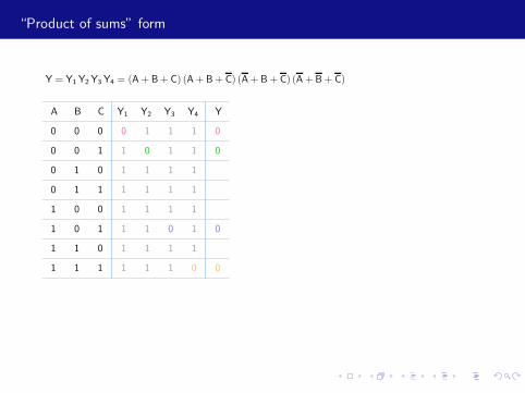
Y = Y1 Y2 Y3 Y4 = (A+ B+ C) (A+ B+ C) (A+ B+ C) (A+ B+ C)
0
0
0
0
1
1
1
1
0
0
0
0
1
1
1
1
0
0
1
1
0
0
1
1
0
1
1
1
1
1
1
1
0
1
1
1
1
1
1
1
0
1
1
1
1
1
1
1 0
1
1
1
1
1
1
1
0
0
0
0
1
1
1
1
Note that Y is identical to X (seen two slides back). This is an example of how the same function
can be written in two seemingly different forms (in this case, the sum-of-products form and the
product-of-sums form).
M. B. Patil, IIT Bombay

“Product of sums” form
YCBA Y4Y3Y2Y1
Y = Y1 Y2 Y3 Y4 = (A+ B+ C) (A+ B+ C) (A+ B+ C) (A+ B+ C)
0
0
0
0
1
1
1
1
0
0
0
0
1
1
1
1
0
0
1
1
0
0
1
1
0
1
1
1
1
1
1
1
0
1
1
1
1
1
1
1
0
1
1
1
1
1
1
1
0
1
1
1
1
1
1
1
0
0
0
0
1
1
1
1
Note that Y is identical to X (seen two slides back). This is an example of how the same function
can be written in two seemingly different forms (in this case, the sum-of-products form and the
product-of-sums form).
M. B. Patil, IIT Bombay

“Product of sums” form
YCBA Y4Y3Y2Y1
Y = Y1 Y2 Y3 Y4 = (A+ B+ C) (A+ B+ C) (A+ B+ C) (A+ B+ C)
0
0
0
0
1
1
1
1
0
0
0
0
1
1
1
1
0
0
1
1
0
0
1
1
0
1
1
1
1
1
1
1
0
1
1
1
1
1
1
1
0
1
1
1
1
1
1
1 0
1
1
1
1
1
1
1
0
0
0
0
1
1
1
1
Note that Y is identical to X (seen two slides back). This is an example of how the same function
can be written in two seemingly different forms (in this case, the sum-of-products form and the
product-of-sums form).
M. B. Patil, IIT Bombay

“Product of sums” form
YCBA Y4Y3Y2Y1
Y = Y1 Y2 Y3 Y4 = (A+ B+ C) (A+ B+ C) (A+ B+ C) (A+ B+ C)
0
0
0
0
1
1
1
1
0
0
0
0
1
1
1
1
0
0
1
1
0
0
1
1
0
1
1
1
1
1
1
1
0
1
1
1
1
1
1
1
0
1
1
1
1
1
1
1 0
1
1
1
1
1
1
1
0
0
0
0
1
1
1
1
Note that Y is identical to X (seen two slides back). This is an example of how the same function
can be written in two seemingly different forms (in this case, the sum-of-products form and the
product-of-sums form).
M. B. Patil, IIT Bombay

Standard sum-of-products form
Consider a function X of three variables A, B, C :
X = AB C + AB C + AB C
This form is called the standard sum-of-products form, and each individual term(consisting of all three variables) is called a “minterm.”
In the truth table for X , the numbers of 1s is the same as the number of minterms, aswe have seen in an example.
X can be rewritten as,
X = AB C + AB (C + C)
= AB C + AB.
This is also a sum-of-products form, but not the standard one.
M. B. Patil, IIT Bombay
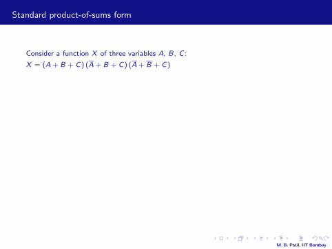
Standard product-of-sums form
Consider a function X of three variables A, B, C :
X = (A + B + C) (A + B + C) (A + B + C)
This form is called the standard product-of-sums form, and each individual term(consisting of all three variables) is called a “maxterm.”
In the truth table for X , the numbers of 0s is the same as the number of maxterms, aswe have seen in an example.
X can be rewritten as,
X = (A + B + C) (A + B + C) (A + B + C)
= (A + B + C) (A + C + B) (A + C + B)
= (A + B + C) (A + C + B B)
= (A + B + C) (A + C).
This is also a product-of-sums form, but not the standard one.
M. B. Patil, IIT Bombay

The “don’t care” condition
I want to design a box (with inputs A, B, C , and output S) which will help in scheduling myappointments.
A ≡ I am in town, and the time slot being suggested for the appointment is free.
B ≡ My favourite player is scheduled to play a match (which I can watch on TV).
C ≡ The appointment is crucial for my business.
S ≡ Schedule the appointment.
The following truth table summarizes the expected functioning of the box.
A B C S
0 X X 0
1 0 X 1
1 1 0 0
1 1 1 1
Note that we have a new entity called X in the truth table.
X can be 0 or 1 (it does not matter) and is therefore called the “don’t care” condition.
Don’t care conditions can often be used to get a more efficient implementation of a logicalfunction.
M. B. Patil, IIT Bombay