EE 3054: Signals, Systems, and Transforms

Lab Manual

1. The lab will meet every week.

2. Be sure to review the lab ahead of the lab session. Please ask questions of the TA’s if you need

some help, but also, please prepare in advance for the labs by reading the lab closely.

3. Your activity, participation, and progress during the lab session will be part of your lab grade.

(Don’t browse the web during lab!)

4. The lab consists of computer-based exercises. You are required to bring your laptop computer to

lab with MATLAB installed. In case you do not have MATLAB installed on your laptop computer

you can go to the laptop help desk to have it installed. You will need the Signal Processing

Toolbox.

5. Labs and the data files required for some labs will be available on the web at:

http://taco.poly.edu/selesi/EE3054/lab/

6. A lab report for each lab (except for Lab 1) will be due the following week in lab. Your lab report

should include relevant code fragments, figures, answers to discussion questions in the lab, and

explanations. No report is required for Lab 1.

7. There will be at least two paper/pencil quizzes related to the lab during the semester. The first

lab quiz will be early in the semester and will focus on MATLAB usage only. The second lab

quiz will be later in the semester and will cover concepts from the labs and lecture and MATLAB

programming.

At the end of this lab manual, there is an example quiz 1. You should be able to answer all the

questions on this example quiz before taking the first MATLAB quiz.

8. The earlier in the semester you become comfortable with MATLAB the better. The first lab

introduces you to MATLAB. You must go through the tutorial Getting Started with MATLAB.

Be sure to download this tutorial to your computer as soon as possible. This tutorial can be

downloaded for free from the Mathworks website:

http://www.mathworks.com/access/helpdesk/help/pdf doc/matlab/getstart.pdf

Other documentation can be obtained at:

1

http://www.mathworks.com/access/helpdesk/help/helpdesk.shtml

For convenience, the MATLAB tutorial is also available at:

http://taco.poly.edu/selesi/EE3054/lab/

9. There is a MATLAB book in the book store which will help you learn MATLAB.

10. In preparation for some of the labs you should read the additional lab notes. These additional

notes for the lab are contained in the pdf file: ”AddLabNotes.pdf” available on the lab web site.

Prepared by Ivan Selesnick, 2004.

2

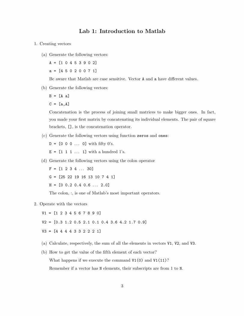
Lab 1: Introduction to Matlab

1. Creating vectors

(a) Generate the following vectors:

A = [1 0 4 5 3 9 0 2]

a = [4 5 0 2 0 0 7 1]

Be aware that Matlab are case sensitive. Vector A and a have different values.

(b) Generate the following vectors:

B = [A a]

C = [a,A]

Concatenation is the process of joining small matrices to make bigger ones. In fact,

you made your first matrix by concatenating its individual elements. The pair of square

brackets, [], is the concatenation operator.

(c) Generate the following vectors using function zeros and ones:

D = [0 0 0 . . . 0] with fifty 0’s.

E = [1 1 1 . . . 1] with a hundred 1’s.

(d) Generate the following vectors using the colon operator

F = [1 2 3 4 . . . 30]

G = [25 22 19 16 13 10 7 4 1]

H = [0 0.2 0.4 0.6 . . . 2.0]

The colon, :, is one of Matlab’s most important operators.

2. Operate with the vectors

V1 = [1 2 3 4 5 6 7 8 9 0]

V2 = [0.3 1.2 0.5 2.1 0.1 0.4 3.6 4.2 1.7 0.9]

V3 = [4 4 4 4 3 3 2 2 2 1]

(a) Calculate, respectively, the sum of all the elements in vectors V1, V2, and V3.

(b) How to get the value of the fifth element of each vector?

What happens if we execute the command V1(0) and V1(11)?

Remember if a vector has N elements, their subscripts are from 1 to N.

3

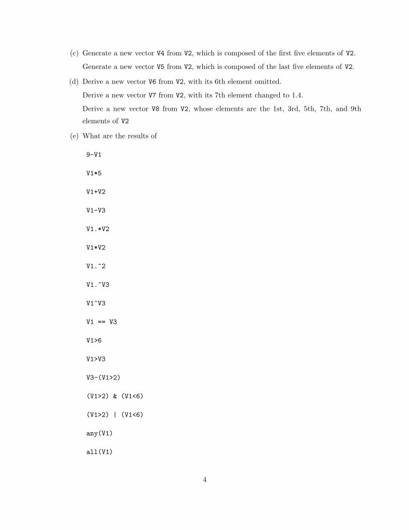
(c) Generate a new vector V4 from V2, which is composed of the first five elements of V2.

Generate a new vector V5 from V2, which is composed of the last five elements of V2.

(d) Derive a new vector V6 from V2, with its 6th element omitted.

Derive a new vector V7 from V2, with its 7th element changed to 1.4.

Derive a new vector V8 from V2, whose elements are the 1st, 3rd, 5th, 7th, and 9th

elements of V2

(e) What are the results of

9-V1

V1*5

V1+V2

V1-V3

V1.*V2

V1*V2

V1.^2

V1.^V3

V1^V3

V1 == V3

V1>6

V1>V3

V3-(V1>2)

(V1>2) & (V1<6)

(V1>2) | (V1<6)

any(V1)

all(V1)

4

3. Using Matlab help system, click on

Help -> MATLAB help

or type helpdesk to can open the help files. For description of a single function or command,

type

help command_name

on the command line, or use ’search’ in the help window.

For example, type

help plot

on the command line.

4. Flow control

What are the results of these sets of commands? Think them over and run them with Matlab

to see if you are right.

(a) A = zeros(1,5);

for n = 1:4

for m = 1:3

A = A + n*m;

end

end

A

(b) B = [1 0];

if (all(B))

B = B + 1;

else if (any(B))

B = B + 2;

else

B = B + 3;

end

B

5

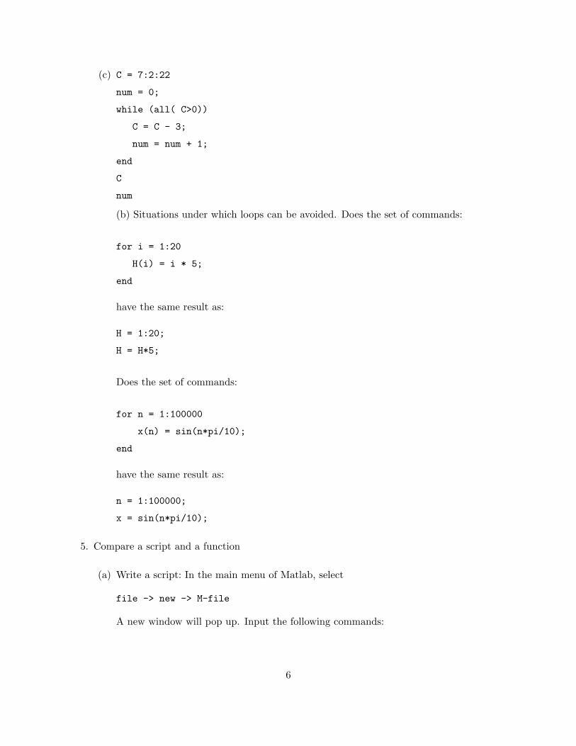
(c) C = 7:2:22

num = 0;

while (all( C>0))

C = C - 3;

num = num + 1;

end

C

num

(b) Situations under which loops can be avoided. Does the set of commands:

for i = 1:20

H(i) = i * 5;

end

have the same result as:

H = 1:20;

H = H*5;

Does the set of commands:

for n = 1:100000

x(n) = sin(n*pi/10);

end

have the same result as:

n = 1:100000;

x = sin(n*pi/10);

5. Compare a script and a function

(a) Write a script: In the main menu of Matlab, select

file -> new -> M-file

A new window will pop up. Input the following commands:

6

x = 1:5;

y = 6:10;

g = x+y;

and then save the file as myscript.m under the default path matlab/work

(b) Write a function: Create a new m file following the procedure of above. Type in the

commands:

function g = myfunction(x,y)

g = x + y;

and then save it as myfunction.m

(c) Compare their usage

(1) run the commands one by one:

myscript

x

y

g

z = myscript (error?)

(2) Run command clear to remove all variables from memory

(3) Run the commands one by one:

x = 1:5;

y = 6:10;

myfunction (error?)

z = myfunction(x,y)

g (error?)

a = 1:10;

b = 2:11;

myfunction(a,b)

Can you explain what is going on here?

7

Lab 2: Basic Plotting of Signals

Using MATLAB, make plots of the signals below. Put your code in a Matlab script file so you

can rerun it from the Matlab command after you make revisions to your file.

Use the subplot command to put several plots on the same page. Print out the plots and turn

them in with your code. Use help subplot to find out how to use the command.

Use the plot command to plot continuous-time signals. Use the stem command to plot discrete-

time signals. Use help plot and help stem to find out how to use these commands. Our conven-

tion is that f(t) denotes a continuous-time signal, and that f(n) denotes a discrete-time signal.

1. Plotting Continuous-Time Signals

For the following: Run the following three lines and explain why the plots are different.

t = 0:2*pi; plot(t,sin(t))

t = 0:0.2:2*pi; plot(t,sin(t))

t = 0:0.02:2*pi; plot(t,sin(t))

For the last graph, add a title and axis labels with:

title(’My Favorite Function’)

xlabel(’t (Seconds)’)

ylabel(’y(t)’)

Change the axis with:

axis([0 2*pi -1.2 1.2])

Put two plots on the same axis:

t = 0:0.2:2*pi; plot(t,sin(t),t,sin(2*t))

Produce a plot with out connecting the points:

t = 0:0.2:2*pi; plot(t,sin(t),’.’)

Try the following command:

t = 0:0.2:2*pi; plot(t,sin(t),t,sin(t),’r.’)

What does the r do?

8

2. Plotting Discrete-Time Signals

Use stem to plot the discrete-time step-function:

n = -10:10;

f = n >= 0;

stem(n,f)

Make stem plots of the following signals. Decide for yourself what the range of n should be.

f(n) = u(n)− u(n− 4)

g(n) = n · u(n)− 2 (n− 4) · u(n− 4) + (n− 8) · u(n− 8)

x(n) = δ(n)− 2 δ(n− 4)

y(n) = (0.9)n (u(n)− u(n− 20))

v(n) = cos(0.12 πn) u(n)

3. The conv Command

Use help conv to find out how to use the conv command.

Let

f(n) = u(n)− u(n− 4)

g(n) = n · u(n)− 2 (n− 4) · u(n− 4) + (n− 8) · u(n− 8).

Make stem plots of the following convolutions. Use the MATLAB conv command to compute

the convolutions.

(a) f(n) ∗ f(n)

(b) f(n) ∗ f(n) ∗ f(n)

(c) f(n) ∗ g(n)

(d) g(n) ∗ δ(n)

(e) g(n) ∗ g(n)

Comment on your observations: Do you see any relationship between f(n) ∗ f(n) and g(n) ?

Compare f(n) with f(n)∗f(n) and with f(n)∗f(n)∗f(n). What happens as you repeatedly

convolve this signal with itself?

Use the commands title, xlabel, ylabel to label the axes of your plots.

9

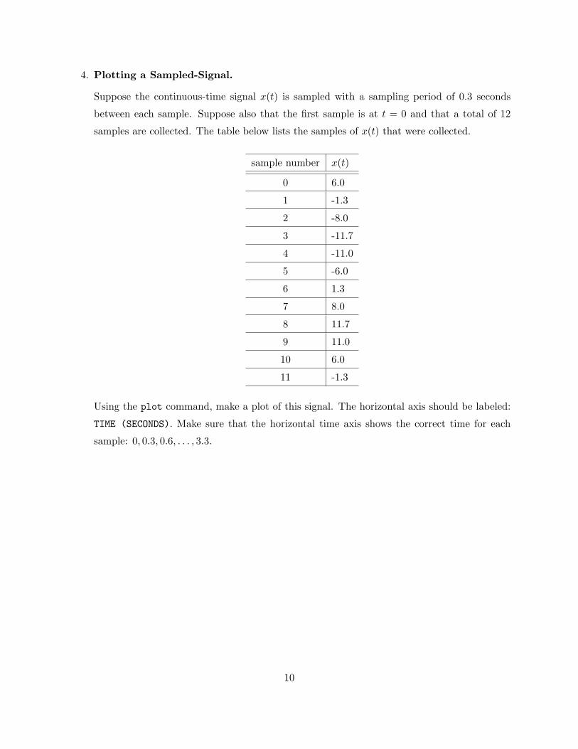
4. Plotting a Sampled-Signal.

Suppose the continuous-time signal x(t) is sampled with a sampling period of 0.3 seconds

between each sample. Suppose also that the first sample is at t = 0 and that a total of 12

samples are collected. The table below lists the samples of x(t) that were collected.

sample number x(t)

0 6.0

1 -1.3

2 -8.0

3 -11.7

4 -11.0

5 -6.0

6 1.3

7 8.0

8 11.7

9 11.0

10 6.0

11 -1.3

Using the plot command, make a plot of this signal. The horizontal axis should be labeled:

TIME (SECONDS). Make sure that the horizontal time axis shows the correct time for each

sample: 0, 0.3, 0.6, . . . , 3.3.

10

Lab 3: Smoothing Data and Difference Equations

1. Convolution of Non-Causal Signals

Use Matlab to make stem plots of the following signals. Decide for yourself what the range

of n should be. Note that both of these signals start to the left of n = 0.

f(n) = 3 δ(n + 2)− δ(n− 1) + 2 δ(n− 3)

g(n) = u(n + 4)− u(n− 3)

Next, use Matlab to make a stem plot of x(n) = f(n) ∗ g(n).

Also: plot the signals by hand without relying on Matlab and check that you get the same

result as your Matlab plot (not to turn in).

To turn in: The plots of f(n), g(n), x(n), and your Matlab commands to create these signals

and plots.

2. Smoothing Data

Save the data file DataEOG.txt from the course website. Load the data into Matlab using the

command load DataEOG.txt Type whos to see your variables. One of the variables will be

DataEOG. For convenience, rename it to x by typing: x = DataEOG; This signal comes from

measuring electrical signals from the brain of a human subject.

Make a stem plot of the signal x(n). You will see it doesn’t look good because there are

so many points. Make a plot of x(n) using the plot command. As you can see, for long

signals we get a better plot using the plot command. Although discrete-time signals are

most appropriately displayed with the stem command, for long discrete-time signals (like this

one) we use the plot command for better appearance.

Create a simple impulse response for an LTI system:

h = ones(1,11)/11;

Make a stem plot of the impulse response.

Find the output signal y(n) of the system when x(n) is the input (using the conv command).

Make plot of the output y(n).

(a) What is the effect of the convolution in this example?

(b) How is the length of y(n) related to the length of (n)

11

(c) Plot x(n) and y(n) on the same graph. What problem do you see? Can you get y(n) to

“line up” with x(n)?

(d) Use the following commands:

y2 = y;

y2(1:5) = [];

y2(end-4:end) = [];

What is the effect of these commands? What is the length of y2? Plot x and y2 on the

same graph. What do you notice now?

(e) Repeat the problem, but use a different impulse response:

h = ones(1,31)/31;

What should the parameters in part (d) be now?

(f) Repeat the problem, but use

h = ones(1,67)/67;

What should the parameters in part (d) be now?

Comment on your observations.

To turn in: The plots, your Matlab commands to create the signals and plots, and discussion.

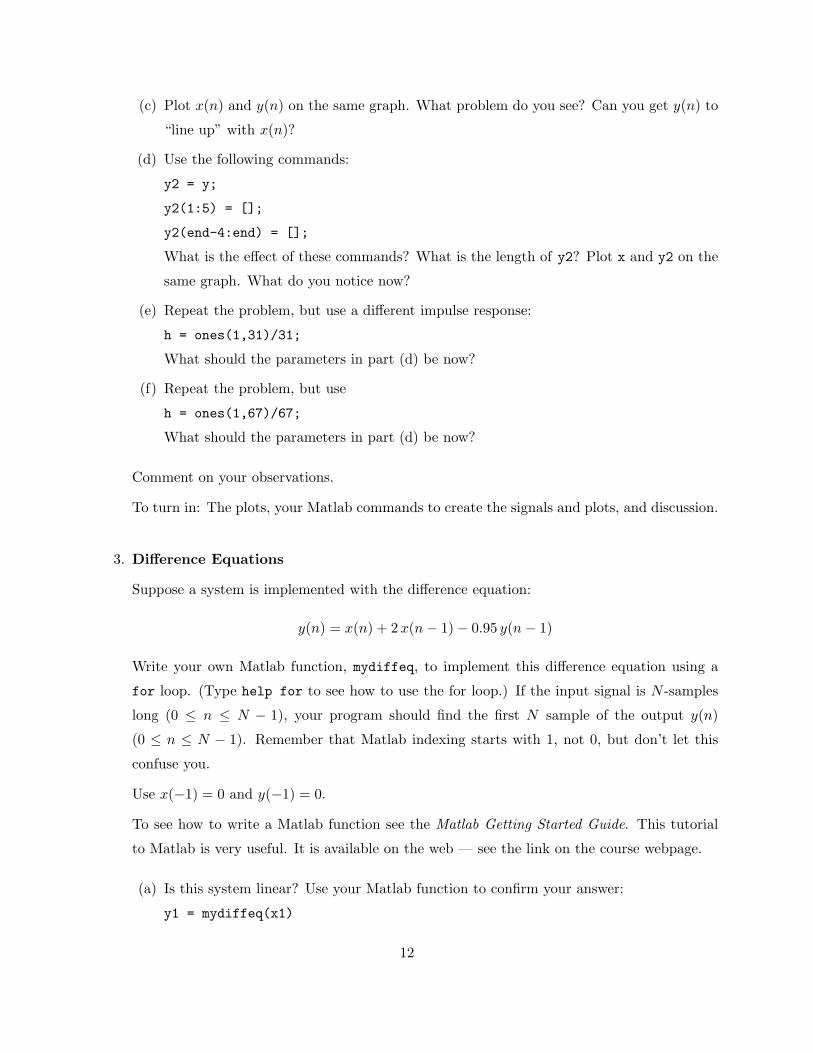
3. Difference Equations

Suppose a system is implemented with the difference equation:

y(n) = x(n) + 2 x(n− 1)− 0.95 y(n− 1)

Write your own Matlab function, mydiffeq, to implement this difference equation using a

for loop. (Type help for to see how to use the for loop.) If the input signal is N -samples

long (0 ≤ n ≤ N − 1), your program should find the first N sample of the output y(n)

(0 ≤ n ≤ N − 1). Remember that Matlab indexing starts with 1, not 0, but don’t let this

confuse you.

Use x(−1) = 0 and y(−1) = 0.

To see how to write a Matlab function see the Matlab Getting Started Guide. This tutorial

to Matlab is very useful. It is available on the web — see the link on the course webpage.

(a) Is this system linear? Use your Matlab function to confirm your answer:

y1 = mydiffeq(x1)

12

y2 = mydiffeq(x2)

y3 = mydiffeq(x1+2*x2)

Use any signals x1, x2 you like.

(b) Is this system time-invariant? Confirm this in Matlab (how?).

(c) Compute and plot the impulse response of this system. Use x = [1, zeros(1,100)];

as input.

(d) Define x(n) = cos(π n/8) [u(n) − u(n − 50)]. Compute the output of the system in two

ways:

(1) y(n) = h(n) ∗ x(n) using the conv command.

(2) Use your function to find the output for this input signal.

Are the two output signals you compute the same?

(e) Write a new Matlab function for the system with the difference equation:

y(n) = x(n) + 2 x(n− 1)

Find and plots the impulse response of this system. What is the difference between the

two impulse responses?

(f) Write a new Matlab function for the system with the difference equation:

y(n) = x(n) + 2 x(n− 1)− 1.1 y(n− 1)

Find and plots the impulse response of this system. What do you find? Discuss your

observations.

To turn in: The plots, your Matlab commands to create the signals and plots, and discussion.

13

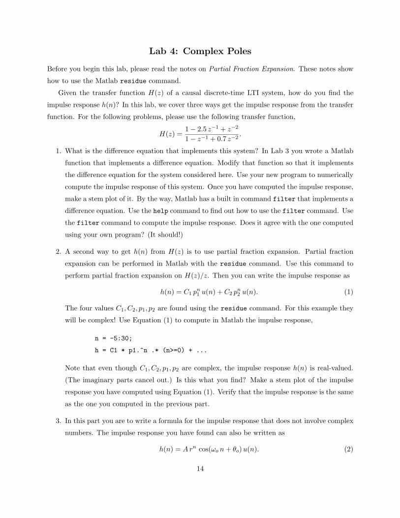
Lab 4: Complex Poles

Before you begin this lab, please read the notes on Partial Fraction Expansion. These notes show

how to use the Matlab residue command.

Given the transfer function H(z) of a causal discrete-time LTI system, how do you find the

impulse response h(n)? In this lab, we cover three ways get the impulse response from the transfer

function. For the following problems, please use the following transfer function,

H(z) =1− 2.5 z−1 + z−2

1− z−1 + 0.7 z−2.

1. What is the difference equation that implements this system? In Lab 3 you wrote a Matlab

function that implements a difference equation. Modify that function so that it implements

the difference equation for the system considered here. Use your new program to numerically

compute the impulse response of this system. Once you have computed the impulse response,

make a stem plot of it. By the way, Matlab has a built in command filter that implements a

difference equation. Use the help command to find out how to use the filter command. Use

the filter command to compute the impulse response. Does it agree with the one computed

using your own program? (It should!)

2. A second way to get h(n) from H(z) is to use partial fraction expansion. Partial fraction

expansion can be performed in Matlab with the residue command. Use this command to

perform partial fraction expansion on H(z)/z. Then you can write the impulse response as

h(n) = C1 pn1 u(n) + C2 pn

2 u(n). (1)

The four values C1, C2, p1, p2 are found using the residue command. For this example they

will be complex! Use Equation (1) to compute in Matlab the impulse response,

n = -5:30;

h = C1 * p1.^n .* (n>=0) + ...

Note that even though C1, C2, p1, p2 are complex, the impulse response h(n) is real-valued.

(The imaginary parts cancel out.) Is this what you find? Make a stem plot of the impulse

response you have computed using Equation (1). Verify that the impulse response is the same

as the one you computed in the previous part.

3. In this part you are to write a formula for the impulse response that does not involve complex

numbers. The impulse response you have found can also be written as

h(n) = A rn cos(ωo n + θo) u(n). (2)

14

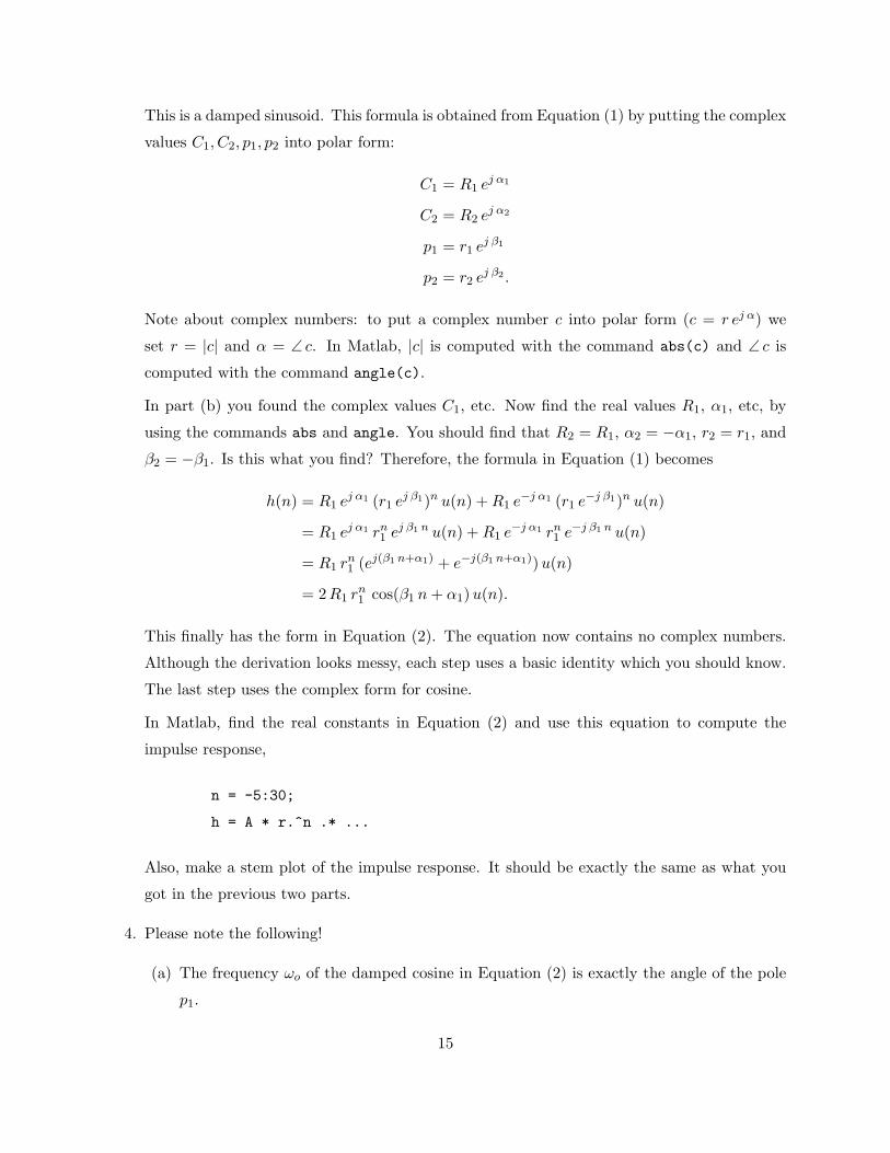
This is a damped sinusoid. This formula is obtained from Equation (1) by putting the complex

values C1, C2, p1, p2 into polar form:

C1 = R1 ej α1

C2 = R2 ej α2

p1 = r1 ej β1

p2 = r2 ej β2 .

Note about complex numbers: to put a complex number c into polar form (c = r ej α) we

set r = |c| and α = ∠ c. In Matlab, |c| is computed with the command abs(c) and ∠ c is

computed with the command angle(c).

In part (b) you found the complex values C1, etc. Now find the real values R1, α1, etc, by

using the commands abs and angle. You should find that R2 = R1, α2 = −α1, r2 = r1, and

β2 = −β1. Is this what you find? Therefore, the formula in Equation (1) becomes

h(n) = R1 ej α1 (r1 ej β1)n u(n) + R1 e−j α1 (r1 e−j β1)n u(n)

= R1 ej α1 rn1 ej β1 n u(n) + R1 e−j α1 rn

1 e−j β1 n u(n)

= R1 rn1 (ej(β1 n+α1) + e−j(β1 n+α1)) u(n)

= 2R1 rn1 cos(β1 n + α1) u(n).

This finally has the form in Equation (2). The equation now contains no complex numbers.

Although the derivation looks messy, each step uses a basic identity which you should know.

The last step uses the complex form for cosine.

In Matlab, find the real constants in Equation (2) and use this equation to compute the

impulse response,

n = -5:30;

h = A * r.^n .* ...

Also, make a stem plot of the impulse response. It should be exactly the same as what you

got in the previous two parts.

4. Please note the following!

(a) The frequency ωo of the damped cosine in Equation (2) is exactly the angle of the pole

p1.

15

(b) The decay of the damped cosine depends on r which is exactly the absolute value (mod-

ulus) of the pole p1.

Therefore, the locations of the poles of an LTI system provides information about the form

of the impulse response.

To make a diagram of the poles and zeros of the system, use the zplane command.

zplane(b,a)

where b and a are the same vectors used for the filter and residue commands. (Note:

when using zplane the vectors b and a must be row vectors. If they are column vectors you

must take the transpose of them to get row vectors.)

Make a diagram of the poles and zeros of the above system using zplane.

5. The system considered above was a very simple one. For additional practice, take the transfer

function

H(z) =1− 0.6 z−1

1− 2.1 z−1 + 1.6 z−2 − 0.4 z−3.

For this system repeat the previous parts. For this system Equation (1) will have three

components instead of two. Equation (2) will have an extra term:

h(n) = A rn cos(ωo n + θo) u(n) + B pn3 u(n).

To turn in: the plots you produced, the Matlab code to produce the plots and intermediate results

(show your use of the residue and filter commands). Also include discussion of your observations,

explanation of your steps, and derivation of the impulse response in Equation (1).

16

Lab 5: Frequency Responses

Consider a causal discrete-time LTI system implemented using the difference equation,

y(n) = 0.1 x(n)− 0.1176 x(n− 1) + 0.1 x(n− 2) + 1.7119 y(n− 1)− 0.81 y(n− 2)

For convenience, the frequency response of the system, H(ej ω), is sometimes denoted Hf (ω).

1. What is the transfer function H(z) of the system? (Not a Matlab question!)

2. Plot the magnitude of the frequency response Hf (ω) of the system using the Matlab command

freqz:

>> [H,w] = freqz(b,a);

>> plot(w,abs(H));

where b and a are appropriately defined.

3. When the input signal is

x(n) = cos(0.1 π n) u(n) (3)

find the output signal y(n) using the Matlab command filter. Use n = 0, 1, 2, . . . , 100.

Make a stem plot of the input and output signals. Use subplot(2,1,1) for x(n) and

subplot(2,1,2) for y(n). Comment on your observations. How could y(n) be predicted

from the frequency response of the system?

4. Lets find the exact value of Hf (ω) at ω = 0.1 π. First, express Hf (0.1 π) as

Hf (0.1 π) =B(ej 0.1 π)A(ej 0.1 π)

where B(z) and A(z) are polynomials. Second, use the exp command to find the complex

number z = ej 0.1 π. Third, evaluate B(z) and A(z) at the complex value z = ej 0.1 π using the

Matlab command polyval. (Use help to see how to use this command.)

5. Recall that when the input signal x(n) is

x(n) = cos(0.1 π n)

then the output signal is

y(n) = |Hf (0.1 π)| cos(0.1 π n + ∠Hf (0.1 π)).

17

(Assuming that the impulse response h(n) is real.) Here is the general diagram:

cos(ωo n) −→ h(n) −→ |Hf (ωo)| cos(ωo n + ∠Hf (ωo))

Note that this input signal x(n) starts at n = −∞. (There is no u(n) term.) However, we are

interested here in the case when x(n) starts at n = 0, namely when x(n) is given by Equation

(3). In this case, we have

cos(ωo n) u(n) −→ h(n) −→ |Hf (ωo)| cos(ωo n + ∠Hf (ωo))u(n) + Transients

The transients die out, and the steady-state output signal is simply |Hf (ωo)| cos(ωo n +

∠Hf (ωo))u(n).

In Matlab, create a stem plot of the steady-state output signal

s(n) = |Hf (0.1 π)| cos(0.1 π n + ∠Hf (0.1 π))

Compare your plot of s(n) with your plot of y(n) you computed using the filter command.

You can do this by plotting them on the same graph with

plot(n,y,n,s)

(stem does not make multiple plots on the same graph, so we use must plot here.) You should

find that s(n) and y(n) agree after a while. (After the transient response has died out.) Is

this what you find? After the transient response has died out, the steady-state output signal

s(n) remains.

6. When the input signal is

x(n) = cos(0.3 π n) u(n)

find the output signal y(n) using the Matlab command filter. Use n = 0, 1, 2, . . . , 100.

Make a stem plot of the input and output signals. Use subplot(2,1,1) for x(n) and

subplot(2,1,2) for y(n). Comment on your observations. How could y(n) be predicted

from the frequency response of the system? What is the steady-state signal? Relate your

explanation to the concept describe in the previous question.

7. Plot the poles and zeros of the transfer function using the Matlab command zplane:

zplane(b,a)

Comment on how the frequency response magnitude |Hf (ω)| can be predicted from the pole-

zero diagram.

18

8. Some Simple Systems

For the causal discrete-time LTI systems implemented by each of the following difference

equations plot the frequency response magnitude |Hf (ω)|, the pole-zero diagram, and the

impulse response.

y(n) = x(n) + 1.8 y(n− 1)− 0.9 y(n− 2) (4)

y(n) = x(n) + 1.6 y(n− 1)− 0.72 y(n− 2) (5)

y(n) = x(n) + 1.53 y(n− 1)− 0.9 y(n− 2) (6)

y(n) = x(n) + 1.4 y(n− 1) + 0.72 y(n− 2) (7)

y(n) = x(n)− 0.85 y(n− 1) (8)

y(n) = x(n)− 0.95 y(n− 1) (9)

Comment on your observations: How can you predict from the pole-zero diagram what the

frequency response will look like and what the impulse response will look like? (Remember

the partial fraction expansion procedure.)

Suppose you were given a diagram of each of the pole-zero diagrams, frequency responses,

and impulse responses, but that they were out of order. Could you match each diagram to

the others (without doing any computation)?

9. Placing the Zeros and Poles

In this part of the lab, you are to derive the difference equation of a system that has the poles

and zeros you want it to have. Suppose you want a 3rd order LTI system with the following

poles and zeros.

p1 = 0.8 ej0.2 π, p2 = 0.8 e−j0.2 π, p3 = 0.7, z1 = −1, z2 = ej0.6 π, z3 = e−j0.6 π

Use the poly command in Matlab to find B(z) and A(z) from the zero and poles. This gives

b and a from which you can write down the difference equation. Also make a stem plot of the

impulse response and frequency response magnitude. You can use zplane to plot the pole

and zeros of the system. This way you can verify that the system you derived has the poles

and zeros you designed it to have.

Now change the poles p1 and p2 to

p1 = 0.98 ej0.2 π, p2 = 0.98 e−j0.2 π,

19

find the new difference equation, and plot the impulse response and frequency response mag-

nitude.

How does this change to the position of the poles affect the nature of the impulse response

of the system and the frequency response?

To turn in: The plots you produced, your Matlab commands to produce the plots, and your

discussion of your observations.

20

Lab 6: Recursive Digital Filters

Please carefully read the notes on Recursive Digital Filters before the lab.

1. Use the Matlab function ellip to obtain a 3rd order digital filter with pass-band ripple

δp = 0.01, stop-band ripple δs = 0.01, and cut-off frequency 0.4 π. [That means, use Wn =

0.4 in ellip.] You will need to convert δp, δs to Rp and Rs. Make a plot of the magnitude of

the frequency response, on a linear scale and in dB, and of the impulse response. Also make

a plot of the pole-zero diagram (using zplane).

2. Repeat the previous problem, but instead use a filter of order 4.

3. Repeat the previous problem, but obtain instead a filter of order 6. Comment on your

observations. How does the frequency response of the elliptic filter improve as the filter order

is increased? How does the impulse response change?

4. Read the full help file for ellip. This command can be used to obtain high-pass filters,

band-pass filters, and band-stop filters as well. Design a discrete-time high-pass filter and

plot the frequency response, impulse response, and pole-zero diagram.

5. Design a discrete-time bandpass filter and plot the frequency response, impulse response, and

pole-zero diagram.

6. Other types of IIR digital filters can be design with Matlab. The Butterworth and Chebyshev

filters are commonly used filter types. These filters can be designed in Matlab using the

commands butter, cheby1, cheby2. Use the help command to investigate these filters.

Design a Butterworth low-pass IIR digital low-pass filter of order 4 using butter, and make

the corresponding graphs.

7. Design a Chebyshev-I low-pass IIR digital low-pass filter of order 4 using cheby1, and make

the corresponding graphs.

8. Design a Chebyshev-II low-pass IIR digital low-pass filter of order 4 using cheby2, and make

the corresponding graphs.

To turn in: Graphs of the frequency responses, impulse responses, and pole-zero diagram and

your comments: In what ways do the four types of IIR filters differ (ellip, butter, cheby1, cheby2)?

How do they differ in the frequency response and pole-zero plots? What happens as you increase

the order of these filters?

21

Lab 7: Noise Reduction

Matlab comes with a speech data set of someone saying ‘Matlab’. The Matlab command load

mtlb will load this data set. If your computer supports sound, you can listen to the original signal

with the command soundsc(mtlb). [Type help soundsc to find out how this command works.]

The speech data set was obtained with a sampling frequency of Fs = 7418 Hz. The sampling period

is Ts = 1/Fs.

The signal can be plotted with the following commands.

>> clear, close all

>> load mtlb

>> who

Your variables are:

Fs mtlb

>> L = length(mtlb);

>> plot([1:L]/Fs,mtlb)

>> axis tight

>> xlabel(’TIME (SECONDS)’)

The data set NoisySpeech.txt on the class webpage, shown in the following figure, contains

the mtlb data set corrupted by additive noise.

0 0.05 0.1 0.15 0.2 0.25 0.3 0.35 0.4 0.45 0.5

−3

−2

−1

0

1

2

3

TIME (SECONDS)

NOISY SPEECH SIGNAL

We will call the noisy signal x(n). You are to design a low-pass filter to filter out the noise.

You will try different low-pass filters until you find one that works well.

1. Download the data from the course webpage and make a plot of the data. You should get

the same figure as shown above.

22

To obtain the data file, go to the course webpage and save the file NoisySpeech.txt, then type

load NoisySpeech.txt on the Matlab command line. (You may need to change your Matlab

working directory with the cd command to where-ever you have saved the file. Alternatively,

you can append the directory to the Matlab path with the command path).

Typing load NoisySpeech.txt on the Matlab command line will create a vector called

NoisySpeech. For convenience, type x = NoisySpeech; on the command line so that you

can use x instead of the longer variable name. The command plot([1:L]/Fs,x) will then

display the plot above.

If your computer supports sound, you can listen to the noisy signal x(n) with the command

soundsc(x).

2. Use the dtft command as shown to plot the magnitude of the spectrum of the signal mtlb.

What frequencies are predominant in the speech signal?

The dtft is not a built in Matlab command, you must download it from the course webpage.

DTFT stands for the Discrete-Time Fourier Transform.

>> [M,f] = dtft(mtlb,1/Fs);

>> plot(f,M)

>> xlabel(’FREQUENCY (Hz)’)

>> title(’SPECTRUM of MTLB’)

3. As in the previous part, use the dtft command to plot |Xf (ω)|, the spectrum of the noisy

signal x(n).

Can you identify which part of the spectrum corresponds to the noise and which part corre-

sponds to the speech signal?

Explain how a low-pass filter can remove the high frequency noise.

From the spectrum can you can you estimate what the cut-off frequency for the lowpass filter

should be?

4. Design an appropriate elliptical low-pass filter with the ellip command. Use the filter

command to filter the noisy signal x(n) with the lowpass filter you design.

Try different cut-off frequencies and different values for the stop-band ripple and the pass-

band ripple. Can you remove most of the noise from the noisy signal?

23

Is the noise reduction quality affected more by the size of passband ripple or by the size of

the stopband ripple? (What is more important — that the passband be very close to 1 or

that the stopband be very close to 0? You should try different filter designs and listen to the

results to fine out.)

24

Lab 8: Synthesizing the Sound of a Plucked String

There are several methods for electronically producing the sound of musical instruments. One

method is to record the sound, sample it, and save the samples. This method is computationally

simple and produces naturalistic sounds, however, it requires a lot of memory and lacks flexibility:

For each note, all the samples must be stored in memory. In addition, it is not possible to tune the

notes.

A second method to simulate the sound of a musical instrument is to model the sound as a sum

of cosine signals. This method requires very little memory — only the frequency and amplitude of

each cosine signal. However, this method usually produces somewhat artificial sounds.

A third method is based on physically modelling the instrument using an appropriately designed

system. Methods based on physical modeling can sound realistic, need very little memory, are

tunable, and can be efficiently implemented. In this lab, we investigate a system for simulating the

sound of a plucked string.

K. Karplus and A. Strong described a very simple system for generating a signal which sounds

like a plucked string. This system can be used to synthesize the sound of a guitar. They published

their method in the paper “Digital Synthesis of Plucked-String and Drum Timbres” in the Computer

Music Journal in 1983.

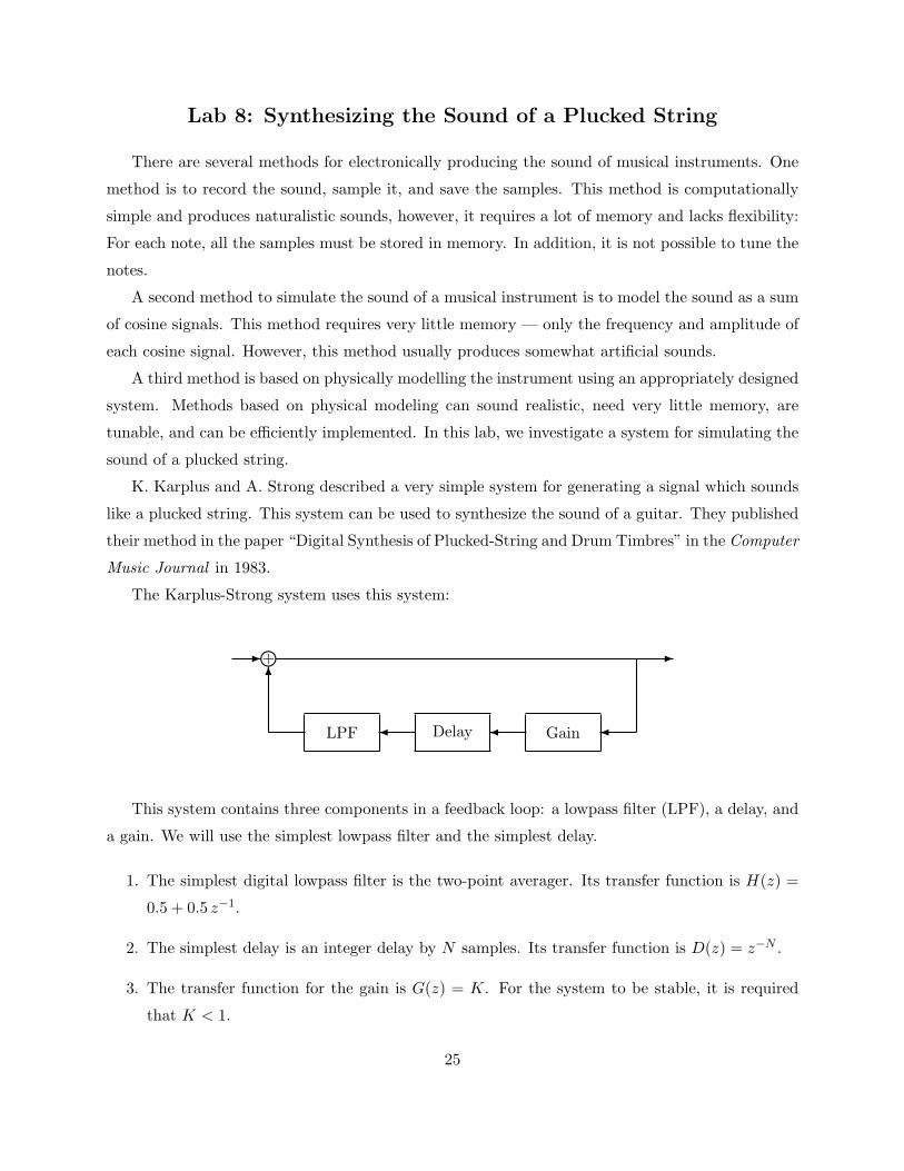
The Karplus-Strong system uses this system:

- -

LPF Delay Gain� � �

6+i

This system contains three components in a feedback loop: a lowpass filter (LPF), a delay, and

a gain. We will use the simplest lowpass filter and the simplest delay.

1. The simplest digital lowpass filter is the two-point averager. Its transfer function is H(z) =

0.5 + 0.5 z−1.

2. The simplest delay is an integer delay by N samples. Its transfer function is D(z) = z−N .

3. The transfer function for the gain is G(z) = K. For the system to be stable, it is required

that K < 1.

25

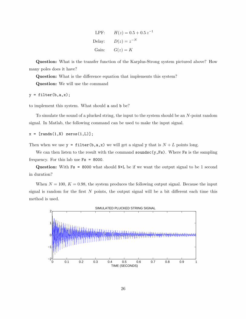
LPF: H(z) = 0.5 + 0.5 z−1

Delay: D(z) = z−N

Gain: G(z) = K

Question: What is the transfer function of the Karplus-Strong system pictured above? How

many poles does it have?

Question: What is the difference equation that implements this system?

Question: We will use the command

y = filter(b,a,x);

to implement this system. What should a and b be?

To simulate the sound of a plucked string, the input to the system should be an N -point random

signal. In Matlab, the following command can be used to make the input signal.

x = [randn(1,N) zeros(1,L)];

Then when we use y = filter(b,a,x) we will get a signal y that is N + L points long.

We can then listen to the result with the command soundsc(y,Fs). Where Fs is the sampling

frequency. For this lab use Fs = 8000.

Question: With Fs = 8000 what should N+L be if we want the output signal to be 1 second

in duration?

When N = 100, K = 0.98, the system produces the following output signal. Because the input

signal is random for the first N points, the output signal will be a bit different each time this

method is used.

0 0.1 0.2 0.3 0.4 0.5 0.6 0.7 0.8 0.9 1−2

−1

0

1

2

TIME (SECONDS)

SIMULATED PLUCKED STRING SIGNAL

26

In Matlab: Write a Matlab program to simulate the sound of a plucked-string using the

Karplus-Strong system above. Use the values N = 100, K = 0.98. Choose L so that the output

signal is one second in duration. Use the filter command. Listen to the output signal using the

soundsc command. Does it sound like a plucked string?

Zoom in on the signal (magnify a small portion of it). Does it look almost periodic?

Run your program several times. Does it sound exactly the same each time?

In Matlab: Plot the frequency response of the system using the freqz command. To ensure

that the plot captures the details of the frequency plot, you can use freqz with a third input

argument, for example:

[H,w] = freqz(b,a,2^16)

plot(w/pi*Fs/2,abs(H))

This will give a denser frequency axis grid.

Question: From the frequency response, how could you have predicted that the output signal

of the Karplus-Strong system is nearly periodic? (Note: the spectrum of a periodic signal is a line

spectrum.)

We can tune the sound by changing the system parameters.

In Matlab: Run the system again, using different values of K. Plot the output signal, listen

to the signal, and plot the frequency response. When you change K what affect does it have on

the output signal and the frequency response?

In Matlab: Run the system again, using different values of N . Plot the output signal, listen

to the signal, and plot the frequency response. When you change N what affect does it have on

the output signal and the frequency response?

Note: The fundamental frequency Fo of the sound produced by this system will depend on the

sampling frequency Fs, the delay N , and the delay incurred by the lowpass filter. It is

Fo =Fs

N + d

where d is the delay of the lowpass filter. The two-point averager has a delay of d = 0.5.

In Matlab: In the above description, we are driving the system with a burst of noise (that

means, the input to the system is a short random signal). Suppose the system is driven by only

an impulse. Run the system with the input x = [1 zeros(1,L)]. (The output will be just the

impulse response of the system.) How does this effect the sound quality of the output signal? Does

it sound more or less natural? Take a close look at the output signal, what do you notice?

27

In Matlab: Suppose the lowpass filter is taken out of the Karplus-Strong system. If the

feedback loop of this system contains only the gain K and the delay z−N then it is called a comb

filter. For the comb filter, what is the difference equation and transfer function? Run the system

without the lowpass filter component. Plot the output signal, listen to the signal, and plot the

frequency response. How does removing the lowpass filter affect the sound and the frequency

response of the system? Why is this system called a comb filter?

Notes:

1. The frequency of the sound produced by the Karplus-Strong system can not be continuously

varied. The delay N must be an integer, so only a discrete set of fundamental frequencies Fo

can be simulated with this model. To overcome this limitation we can introduce a fractional

delay in the feedback loop.

2. If you allow the delay in the feedback loop to be a time-varying delay, then the frequency of

the sound can vary over the duration of the note. Time-varying systems add flexibility.

3. You can learn more about simulating musical instruments using signals and systems on the

web.

http://www.harmony-central.com/Synth/Articles/Physical_Modeling/

28

Lab 9: Stable Inverse Systems and Equalization

1. Suppose that a causal system has the impulse response

h1(n) = 0.5nu(n) (10)

and that an anti-causal system has the impulse response

h2(n) = 3nu(−n− 1). (11)

(a) If these two systems are connected in cascade, what is the transfer function H(z) and

ROC of the total system?

(b) Find the impulse response h(n) of the total system and make a stem plot of h(n) using

Matlab.

(c) Consider the stable inverse G(z) = 1/H(z). Find the ROC of G(z) and g(n). Make a

stem plot g(n) using Matlab. Verify in Matlab that it is an inverse by convolving g(n)

and h(n) to get δ(n). (You will need to truncate h and g first as they are infinite in

length.)

2. Distortion removal. A binary signal is sent over an imperfect channel which introduces

distortion. The channel can be modeled as a discrete-time LTI system with the transfer

function

H(z) =1− 2.5 z−1 + z−2

1− z−1 + 0.7 z−2.

(a) Determine the impulse response g(n) of the stable inverse of H(z). You may use the

residue command in Matlab.

(b) Using Matlab, make a stem plot of h(n), g(n), and h(n) ∗ g(n). Check that you get an

impulse.

(c) Using Matlab (freqz) plot |Hf (ω)| and |Gf (ω)|, the magnitudes of the frequency re-

sponses. Also plot the product |Hf (ω) · Gf (ω)|. What do you expect to get for the

product? Did you get it?

(d) The binary signal x(n) is sent through the channel and the received signal r(n) is shown

in the figure.

29

0 10 20 30 40 50 60 70 80 90 100−3

−2

−1

0

1

2

3

r(n)

n

On the course webpage you will find r(n) contained in the file DistortedSignal.txt,

but not x(n). Download r(n) and make plot of it using Matlab. Filter r(n) with the

impulse response g(n) (use the conv command) and make a plot of the new signal. Has

the distortion been removed? (You should obtain a binary signal.)

(e) Suppose the frequency response Hf (ω) were equal to zero for some frequency ωo. Would

that make the design of an inverse system more difficult? Explain.

30

Lab 10: Echo Cancellation

In this lab you will work on the problem of removing an echo from a recording of a speech

signal. An echo has a couple of parameters: The first parameter is the delay: to seconds (or N

samples). The second parameter is the amplitude of the echo: α.

The lab has the following parts:

1. Create the Echo Signal. You will add an echo to a speech signal.

2. Remove the Echo. You will remove an echo from a speech signal. In this part you know

what the echo parameters to and α are.

3. Estimating Unknown Echo Parameters. You will try to determine the echo parameters

to and α from a speech signal, and then remove the echo.

The lab consists of the following activities and questions:

1. Create the Echo Signal

Load the ‘matlab’ speech signal with the command

>> load mtlb

Then type who to see your variables. You can listen to the signal mtlb with the command

soundsc(mtlb,Fs), provided your computer has a sound card. You should hear the phrase

‘matlab’. For convenience, lets redefine this to be x by typing x = mtlb;.

Make a plot of the signal x versus time (in SECONDS). You will need the sampling frequency

Fs which is loaded when you typed load mtlb. You should find that the speech signal is

about 0.55 seconds in duration.

2. How do you find the exact duration of this signal in seconds?

3. We can create an echo by filtering this signal with the following difference equation:

y(n) = x(n) + α x(n−N)

where x(n) is the echo-free speech signal, which has been delayed by N samples and added

back in with its amplitude scaled by α. This is a reasonable model for an echo resulting from

the signal reflecting off an absorbing surface like a wall. The delay parameter to in seconds

is N/Fs where Fs is the sampling frequency. (Can you explain why?) What is the impulse

response of this system?

31

4. Lets add an echo to the signal with a delay of to = 0.12 seconds and an amplitude of α = 0.8.

What is the delay N in samples? Based on the difference equation, create an echo version of

the signal x using the command y = conv(h,x);. What is h?

Listen to the output of the difference equation. Do you hear the echo?

5. Remove the Echo.

The difference equation above for modeling the echo is an LTI system. To remove the echo, we

need to implement the inverse system. What is the impulse response of the inverse system?

What is the duration of this impulse response?

6. For the echo parameters you used above, plot the impulse response of the inverse system.

Make the horizontal axis in your plot in units of SECONDS.

7. Implement the inverse of the echo system to perform echo cancellation. You can use the

command g = filter(b,a,y). What are the vectors b and a?

8. Listen to the result. Is the echo removed?

9. Estimating Unknown Echo Parameters

In a real problem, you will probably not know what the echo parameters to and α are. You

will need to estimate them from the echo signal itself.

Suppose you are given the data y(n) (which is corrupted by an echo) but suppose you do

not know the value of the delay N . Determine a method of estimating N based on the

autocorrelation function of y(n). Let ryy(n) be the autocorrelation of y(n),

ryy(n) = y(n) ∗ y(−n),

and let rxx(n) be the autocorrelation of x(n),

rxx(n) = x(n) ∗ x(−n).

First, find a formula for the signal ryy(n) in terms of rxx(n) (this is not a Matlab question).

To do this, use the expression you have for the impulse response together with properties of

the convolution sum.

10. Compute in Matlab and plot rxx(n) vs time (in SECONDS). rxx(n) is the autocorrelation of

the echo-free signal. To compute in Matlab the autocorrelation of a signal you can use the

commands

32

>> rxx = conv(x,x(end:-1:1));

or the command xcorr. You should see that it has a peak in the middle.

11. For the signal and echo parameters above, plot ryy(n). Can you determine what the value of

N is from the plot of ryy(n)? (Look at the peaks.) Does it agree with the known value?

12. From the course website, there is a data file you can download for this lab. It contains a

signal which is corrupted by an echo with unknown echo parameters to and α.

Can you estimate N for this data from its autocorrelation?

13. The amplitude α is harder to estimate than N . Once you have estimated N , try to remove

the echo by trying out different values of α and listening to your result. What N and α do

you find work best? Are you able to successfully remove the echo?

14. What if an echo has two components?

y(n) = x(n) + α1 x(n−N1) + α2 x(n−N2)

Discuss what system is required for echo cancellation. How would you find the echo parame-

ters?

33

Lab 11: Fourier Series

1. Find the Fourier series coefficients c(k) for the periodic signal

x(t) = | cos(π t)|.

2. Find the Fourier series coefficients c(k) for the periodic triangular pulse shown below.

x(t)

-�

−5 −4 −3 −2 −1 0 1 2 3 4 5

1

· · ·�

��@@@�

��@@@�

��@@@�

��@@@�

��@@@

· · ·

3. (a) Run the Matlab program fs1.m to see the convergence of the Fourier series of the

periodic pulse signal. The program is available on my.poly.edu.

(b) Write a Matlab program fs2.m to generate the same plots but for the signal x(t) =

| cos(t)|. This entails replacing the line for c0 and ck in fs1.m, with the formula from

question 1.

(c) Write a Matlab program fs3.m to generate the same plots but for the periodic triangular

pulse.

(d) For which signal does the Fourier series converge more rapidly, the periodic rectangular

pulse signal or the periodic triangular signal? How could you predict your answer?

4. Numerical Computation of Fourier Series Coefficients

Sometimes the integration formula for the Fourier series coefficients is difficult to carry out.

In these cases, the coefficients can be obtained numerically. Remember that an integral∫f(t) dt ≈ ∆T

∑m

f(m ∆T )

For example,

c(k) =1T

∫<T>

x(t) e−j k ωo t dt

can be approximated as a sum:

c(k) ≈ ∆T

T

M−1∑m=0

x(m ∆T ) e−j k ωo m (∆T )

34

The following Matlab program computes the first N Fourier series coefficients c(k) numerically

of the signal

x(t) = | cos(π t)|

The program plots the line spectrum (a graph of the FS coefficients). The program also

creates a periodic signal using the calculated coefficients — this verifies if the coefficients

were computed correctly.

Run this program and verify that it works. It can be obtained from my.poly.edu

Change the program so that it computes the Fourier series coefficients of the periodic triangle

wave shown above.

5. The Time-Shift Property

The time-shift property states that if a periodic signal is shifted, then the Fourier coefficients

of that signal are modified according to the following rule: If

x(t) ⇐⇒ c(k)

then

x(t− to) ⇐⇒ e−j k ωo to c(k)

Verify this property numerically using Matlab, by setting

g(t) = | cos(π (t− 0.2))|.

Find the Fourier coefficients of g(t) by first finding the Fourier coefficients of x(t) = | cos(π t)|and modifying those coefficients according to this rule. Then use the new coefficients to

synthesize the periodic signal g(t) by adding up complex exponentials. Are you able to

confirm the time-shift property?

35

EE 3054: Signals, Systems, and Transforms

Example Matlab Quiz

No laptop, no notes, no documentation.

1. Given the following array a,

a =

1 4 2 4

7 5 9 2

-5 7 -2 0

determine the result of each of the following commands.

>> a(2, 3)

>> a(2, :)

>> a(6)

>> a(3, 2:end)

>> a(1:2, 4:-1:2)

>> a([2 2], [2 3])

>> a > 5

>> sum(a)

>> a(:)

>> [a(1,:), a(2,:)]

>> [a(1,:); a(2,:)]

2. What are the results of the following commands?

>> a = [5 2 3 5 8];

>> b = [9 2 5 0 8];

>> a == 5

>> a == b

3. What is the result of each of the following commands?

36

>> a = [zeros(3); ones(1,3)]

>> b = [zeros(3); ones(3,1)]

4. What is the result of the following command?

>> n = 0:0.5:3.2

5. What is the result of the following commands?

>> n = 2:7

>> n(2) = [];

>> n

6. What are all the results of the following commands?

>> a = [3 4; 7 8];

>> b = [1 0; 0 1];

>> a’

>> a - 1

>> a .* b

>> a * b

>> a | b

>> a & b

>> a .^ 2

>> a ^ 2

7. The following code fragment produces 3 graphs. Sketch each of the three graphs.

>> n = 0:7;

>> x = 2*n + 1;

>> stem(n,x)

>> plot(n,x)

>> y = (-1).^n;

>> plot(n,x,n,y)

8. Sketch the 3 graphs produced by the following code.

37

>> n = 0:10;

>> x = (n >= 1) - (n >=5);

>> stem(n,x)

>> h = (n == 5);

>> y = conv(h,x);

>> stem(0:20,y)

>> z = conv(x,x);

>> stem(0:20,z)

9. Write a short Matlab code that will plot a sinusoid of frequency 50 Hz for 10 cycles.

10. The file kiwi.m contains the following:

y = 5;

x = 6;

z = x + y;

The file grape.m contains the following:

function z = grape(x,y)

z = x + y;

What is the result of the following commands?

>> clear

>> x = 2;

>> y = 5;

>> kiwi

>> z

What is the result of the following commands?

>> clear

>> x = 2;

>> y = 5;

>> z = grape(x,y);

>> z

38

EE 3054: Signals, Systems, and Transforms

Lab Quiz 1 — Spring 2005

No laptop, no notes, no documentation.

1. Given the following array a,

a =

9 4 7 2

1 6 3 5

3 10 6 4

determine the result of each of the following commands.

>> a(2, 3)

>> a(0, 2)

>> a(5)

>> a’

>> a(:, [2 2 2])

>> a(1:2:end, 1:2:end)

>> a(end:-1:1, :)

>> max(a)

>> b = a; b([2 3],[1 4]) = [11 22; 33 44]; b

>> b = a; b(:,2) = []; b

>> log10([1 10 100 0.1])

2. What are the results of the following commands?

>> a = [9 4 7 2 8];

>> a(2)

>> a(1,2)

>> a(2,1)

>> a > 5

>> find(a > 5)

>> a * a

39

>> [a, a]

>> [M, k] = min(a); M, k

>> a(1:end-1)

>> a([1 1 1], :)

3. What is the result of each of the following commands?

>> a = [1+j, 1+2*j, 3, 4, 5*j];

>> k = find(imag(a)==0);

>> a(k)

4. What is the result of the following commands?

>> a = [];

>> for k = 5:-1:2

a = [a, k];

end

>> a

5. What is the result of the following commands?

>> a = [-2 3];

>> b = [4 2 -1];

>> conv(a,b)

6. The following code fragment produces 3 graphs. Sketch each of the three graphs.

>> n = 2:0.5:4;

>> x = [3 1 2 0 3];

>> plot(n,x)

>> plot(x)

>> stem(n,x)

7. Write a MATLAB function called over that has one output and two inputs. The first input

is a vector; the second input is a scalar. The output should be the sum of all those elements

in the vector that exceed the scalar. For example,

40

>> over([5 1 3 6 9],4)

ans =

20

because the elements in the vector that are greater than 4 are: 5, 6, and 9, so we have

5 + 6 + 9 = 20.

Your program should not use a for or while loop and it should not use an if statement.

41