Eduardo Enes Cota Toughness Evaluation and Fracture ...

Eduardo Enes Cota

Toughness Evaluation and Fracture Predictions

in Elastoplastic Materials

Dissertação de Mestrado

Dissertation presented to the Programa de Pós–

graduação em Engenharia Mecânica da PUC-Rio in

partial fulfillment of the requirements for the degree of

Mestre em Engenharia Mecânica.

Advisor: Prof. Jaime Tupiassú Pinho de Castro

Rio de Janeiro

February 2019

DBD

PUC-Rio - Certificação Digital Nº 1621880/CA

Eduardo Enes Cota

Toughness Evaluation and Fracture Predictions

in Elastoplastic Materials

Dissertation presented to the Programa de Pós–graduação

em Engenharia Mecânica da PUC-Rio in partial fulfillment of

the requirements for the degree of Mestre em Engenharia

Mecânica. Approved by undersigned Examination

Committee.

Prof. Jaime Tupiassú Pinho de Castro

Advisor

Departamento de Engenharia Mecânica – PUC-Rio

Prof. Marco Antonio Meggiolaro

Departamento de Engenharia Mecânica – PUC-Rio

Prof. Gustavo Henrique Bolognesi Donato

Centro Universitário – FEI

Rio de Janeiro, February 21st, 2019

DBD


All rights reserved.

Eduardo Enes Cota

The former author graduated in Mechanical Engineering from

Pontifícia Universidade Católica do Rio de Janeiro in 2015

Bibliographic data

CDD: 620.11

Enes Cota, Eduardo

Toughness Evaluation and Fracture Predictions in elastic-

plastic Materials / Eduardo Enes Cota; advisor: Jaime Tupiassú

Pinho de Castro. – Rio de Janeiro: PUC-Rio, Departamento de

Engenharia Mecânica, 2019.

v.,110 f: il.color ; 30 cm

Dissertação (mestrado) – Pontifícia Universidade Católica

do Rio de Janeiro, Departamento de Engenharia Mecânica.

Inclui bibliografia

1. Engenharia Mecânica – Teses. 2. Mecânica da Fratura;

. 3. MFEP;. 4. API 5L X80;. 5. Tenacidade;. 6. ASTM E1820;.

7. Integridade Estrutural;. 8. API 579. I. Tupiassú Pinho de

Castro, Jaime. II. Pontifícia Universidade Católica do Rio de

Janeiro. Departamento de Engenharia Mecânica. III. Título.

DBD


Acknowledgement

First of all, I would like to thank my advisor Prof. Jaime Tupiassú Pinho

de Castro for the opportunity, motivation, and guidance during my thesis.

To Prof. Marco Antonio Meggiolaro, Prof. Gustavo Donato, and Prof.

Luis Fernando Martha for the interest in the work and the given advice.

To Prof. Ivan Menezes and Prof. José Freire for all the support.

To my friends from the university João Carlos Virgolino, Rodrigo

Bianchi, Thiago Almeida, Bruno Calasans, and André Xavier.

To my friends from childhood Bruno Fraga, Ian Lange, José Ricardo

Garcia, and Raul Valverde.

To Jullian, Gean, Adrian, Elias, and Euclides for all the help during my

experiments at the laboratories.

To Rodrigo Landin for the specimens machining.

To CNPq for financial support.

To USIMINAS for supplying the material used in the experiments.

To my colleagues and relatives that somehow helped me during this time.

I would also like to do a special thanks to my parents Manuel Julio José Cota

Janeiro, and Rosa Claudia Garrido Enes Cota for all the support and inspiration.

Also, to my sister Larissa, and to my brothers Victor and Raphael Enes Cota.

DBD


Abstract

Enes Cota, Eduardo; Tupiassú Pinho de Castro, Jaime (Advisor).

Toughness Evaluation and Fracture Predictions in elastic- plastic

Materials. Rio de Janeiro, 2019.110p. Dissertação de mestrado –

Departamento de Engenharia Mecânica, Pontifícia Universidade Católica

do Rio de Janeiro.

Understanding how to analyze cracks is essential for the petrochemical

industry to avoid accidents or incidents in a safe and economical way. Structural

Integrity standards provide conservative procedures to assess the actual strength

of cracked components like pipes and pressure vessels. Therefore, critical loads

predictions were computed on a plate with a through-wall crack following level

2 and 3 of the fitness-for-service guide API 579. For comparison, experimental

tests were performed to evaluate the standard conservatism on a ductile tearing

type of failure. Furthermore, the fracture toughness of the steel was measured

through standard JIc tests and material's resistance curves (J-R curve). The

technique used during the fracturing process was the elastic compliance method

with unloading/reloading sequences. Additionally, the effects of the specimen's

geometry and the type of loading, which can significantly change the value of

its toughness, were also analyzed using concepts of elastoplastic fracture

mechanics. The material used in this work was the API 5L X80, which is a High

Strength Low Alloy (HSLA) dual-phase steel developed for deepwater

pipelines. The fracture toughness measurement tests using SE(B) specimens,

which have a medium-to-high plastic constraint, followed the ASTM E1820-17

procedures. The experiments with SE(T) specimens, which present a low plastic

restriction, considered literature procedures.

Keywords

Fracture Mechanics; EPFM; API 5L X80; Toughness; ASTM E1820;

Structural Integrity; API 579

DBD


Resumo

Enes Cota, Eduardo; Tupiassú Pinho de Castro, Jaime (Advisor).

Avaliação da Tenacidade e Previsões de Fraturas em Materiais Elastoplásticos.

Rio de Janeiro, 2019.110p. Dissertação de mestrado – Departamento de

Engenharia Mecânica, Pontifícia Universidade Católica do Rio de

Janeiro.

Compreender como analisar trincas é essencial para a indústria

petroquímica evitar qualquer incidente de uma forma econômica. Normas de

Integridade Estrutural fornecem procedimentos conservadores para avaliar

componentes trincados como tubulações e vasos de pressão. Portanto, previsões

de cargas criticas foram calculadas assumindo uma placa com trinca passante

seguindo procedimentos dos níveis 2 e 3 da API 579. Para comparação, testes

experimentais foram realizados para avaliar o conservatismo da norma em falha

por rasgamento dúctil. Além disso, a tenacidade à fratura foi medida por meio

do JIc e curva J-R. A técnica usada durante o processo de fratura foi o método

de flexibilidade elástica com descarregamento e carregamentos sequenciais.

Adicionalmente, efeito de geometria e tipo de carregamento, os quais possuem

grande influência nas medições de tenacidade, também foram avaliados usando

conceitos da mecânica da fratura elastoplástica. O material utilizado nesse

trabalho foi o API 5L X80, que é um aço de Alta Resistencia e Baixa Liga

(ARBL) bifásico desenvolvido para tubulações aplicáveis em aguas profundas.

Os ensaios experimentais de medição de tenacidade usando corpos de prova

SE(B), que possuem média-alta restrição plástica, foram testados seguindo

procedimentos da ASTM E1820-17. Já os experimentos usando corpos de prova

SE(T), que possuem baixa restrição plástica, foram realizados considerando

procedimentos da literatura.

Palavras-chave

Mecânica da Fratura; MFEP; API 5L X80; Tenacidade; ASTM E1820;

Integridade Estrutural; API 579

DBD


Table of contents

1. Introduction 19

1.1 Disasters 22

1.2 Aim of this study 25

1.3 Motivation 25

1.4 Thesis structure 26

2. Theoretical background 27

2.1 Tensile strength and ductility 27

2.2 Some basic Fracture Mechanics concepts 28

2.2.1 Fracture surfaces 30

2.2.1.1 Ductile fractures 31

2.2.1.2 Brittle fractures 32

2.2.2 Fracture toughness 32

2.3 Linear Elastic Fracture Mechanics (LEFM) fundamentals

33

2.3.1 Stress concentration factor Kt 34

2.3.2 Griffith’s energy approach 34

2.3.3 Energy release rate 35

2.3.4 Stress intensity factors 36

2.3.5 Crack-tip plasticity 38

2.3.6 Crack-tip triaxiality 40

2.4 Elastic-Plastic Fracture Mechanics (EPFM) fundamentals

42

2.4.1 Crack-Tip Opening Displacement (CTOD) 42

2.4.2 J-Integral 43

2.4.3 J-R Curve 44

DBD


2.5 Biparametric fracture mechanics fundamentals 45

2.5.1 T Stress 47

2.5.2 Q Parameter 48

3. Standard procedures to measure fracture toughness 50

3.1 Fracture toughness specimens 50

3.1.1 Fatigue pre-cracking procedures 52

3.1.2 Resistance curve procedures 52

3.1.3 Optical crack size measurements 58

3.2 Procedure for SE(T) specimens 58

4. Experimental procedures and material characterization 61

4.1 Metallography 61

4.2 Chemical analysis 63

4.3 Hardness test 65

4.4 Tensile test 65

4.5 Fracture toughness test 67

4.5.1 SE(B) specimens 68

4.5.2 SE(T) specimens 78

5. Structural integrity assessments 87

5.1 Structure configuration 87

5.2 Predictions by API 579 procedures 88

5.2.1 Level 2 assessments 88

5.2.2 Level 3 assessments 92

5.2.3 Predictions results 93

5.2.3 Validation tests 94

6. Summary of results 97

6.1 Fracture toughness measurements on SE(B) specimens97

6.2 Fracture toughness measurement on SE(T) specimens 98

DBD


6.3 Failure predictions 99

7. Conclusions 100

7.1 Conclusions from the fracture toughness measurements

100

7.2 Conclusions from the failure predictions 102

7.3 Recommendations for future work 103

Bibliography 104

DBD


List of figures

Figure 1.1: Failure behavior [4]. ........................................................... 20

Figure 1.2: Umm Said NGL Plant [17]. ................................................ 22

Figure 1.3: Alexander L. Kielland platform failure [18]. ........................ 23

Figure 1.4: The SS Schenectady broke in two [19]. ............................ 24

Figure 1.5: Comet airplane test [20]. ................................................... 24

Figure 2.1: Typical engineering stress-strain curve [25]. ..................... 28

Figure 2.2: Comparison of (a) strength of materials and (b) fracture

mechanics approach [3]. ...................................................................... 29

Figure 2.3: Basic difference between the validity of LEFM and EPFM

[4]. ........................................................................................................ 29

Figure 2.4: Fracture mechanics [3]. ..................................................... 30

Figure 2.5: Fracture types on tensile tests: a) brittle fracture; b) shear

fracture; c) ductile fracture ; d) perfect ductile fracture [3]. .................. 30

Figure 2.6: Ductile fracture [25]. .......................................................... 31

Figure 2.7: Brittle fracture [25]. ............................................................ 32

Figure 2.8: Modes of cracking [1]. ....................................................... 33

Figure 2.9: Inglis plate [28]. ................................................................. 34

Figure 2.10: Stress field near the tip of a crack [3]. ............................. 37

Figure 2.11: Critical SIF in function of thickness [4]. ........................... 38

Figure 2.12: Plastic zone size [28]. ...................................................... 39

Figure 2.13: Adjusted plastic zone size [28]. ....................................... 40

Figure 2.14: Plastic constraint effect on yield strength [28]. ................ 41

Figure 2.15: Specimen thickness effect on plastic constraint [28]. ...... 41

Figure 2.16: Crack tip opening displacement [29]. .............................. 42

DBD


Figure 2.17: J-Integral [3]. .................................................................... 43

Figure 2.18: J-R Curve for ductile material [3]. .................................... 45

Figure 2.19: Crack size effect on J-R curve [28]. ................................ 46

Figure 2.20: Constraint and geometry influence on fracture toughness

[40]. ...................................................................................................... 47

Figure 2.21: Biaxiality ratio [3]. ............................................................ 48

Figure 3.1: Standard SE(B) specimen [7]. ........................................... 51

Figure 3.2: Standard C(T) specimen [7]. ............................................. 51

Figure 3.3: Standard DC(T) specimen [7]. ........................................... 51

Figure 3.4: Side grooves [28]. .............................................................. 53

Figure 3.5: Compliance technique [28]. ............................................... 54

Figure 3.6: Plastic area [7]. .................................................................. 55

Figure 3.7: J-R curve with constructions lines [7]. ............................... 56

Figure 3.8: Regions for data qualification [7]. ...................................... 57

Figure 4.1: API 5L X80 flat plate. ......................................................... 62

Figure 4.2: Metallographic analysis. .................................................... 63

Figure 4.3: Microstructure of API 5L X80 steel (magnification 500x). . 63

Figure 4.4: Chemical analysis. ............................................................. 63

Figure 4.5: Hardness test. ................................................................... 65

Figure 4.6: Tensile specimens dimensions. ........................................ 65

Figure 4.7: Tensile test. ....................................................................... 66

Figure 4.8: Engineering stress/strain curves. ...................................... 66

Figure 4.9: True stress/strain curves. .................................................. 67

Figure 4.10: SE(B) specimen dimensions in mm. ............................... 68

Figure 4.11: SE(T) specimen dimensions in mm. ................................ 68

Figure 4.12: SE(B) and SE(T) specimens ready for testing. ............... 68

DBD


Figure 4.13: INSTRON 8501 servo-hydraulic testing

machine (100 kN). ............................................................................... 69

Figure 4.14: Pre-crack measurement. ................................................. 70

Figure 4.15: Unloading compliance SE(B)-2 and SE(B)-3. ................. 71

Figure 4.16: Unloading compliance range. .......................................... 71

Figure 4.17: Compliance method calculation. ..................................... 71

Figure 4.18: J-R Curve SE(B)-2. ......................................................... 72

Figure 4.19: J-R Curve SE(B)-3. .......................................................... 72

Figure 4.20: Brittle fracture. ................................................................. 73

Figure 4.21: Unloading compliance SE(B)-4. ...................................... 74





Figure 4.26: Fractography on SE(B)-5 specimen. ............................... 76


Figure 4.28: J-R Curve SE(B)-7. ........................................................ 77


Figure 4.30: MTS 810 servo-hydraulic testing machine (250 kN). ...... 78

Figure 4.31: Unloading compliance SE(B)-9 and SE(B)-10. ............... 78


Figure 4.33: J-R Curve SE(B)-10. ........................................................ 78

Figure 4.34: MTS 1000 kN servo-hydraulic testing machine. .............. 79

Figure 4.35: Unloading compliance SE(T)-2. ...................................... 80

Figure 4.36: SE(T)-2 J-R original. ....................................................... 80

Figure 4.37: SE(T)-2 J-R adjusted. ...................................................... 80


DBD


Figure 4.39: SE(T)-3 J-R original. ....................................................... 81



Figure 4.42: SE(T)-5 J-R original. ..................................................... 82



Figure 4.45: SE(T)-7 J-R original. .................................................... 83



Figure 4.48: SE(T)-8 J-R original. ...................................................... 84


Figure 5.1: Specimen geometry. .......................................................... 87

Figure 5.2: Plate with a through wall crack [12]. .................................. 88

Figure 5.3: Level 1 admissible crack sizes for a flat plate [12]. ........... 88

Figure 5.4: FAD level 2 specified in API 579 guide [12]. ..................... 89

Figure 5.5: Failure analysis diagram level 2 for σm = 100MPa. ........... 91

Figure 5.6: FAD level 2 to find the failure stress σm = 197.6 MPa. ...... 91

Figure 5.7: FAD level 3 [12]. ................................................................ 92

Figure 5.8: FAD level 3 for SE(B)-8, predicting failure under σm = 197.6

MPa. ..................................................................................................... 92

Figure 5.9: Experiment. ....................................................................... 94

Figure 5.10: Plate 1 test. ...................................................................... 95

Figure 5.11: Plate 2 test. ...................................................................... 95

Figure 5.12: Ellipsoidal fatigue 2D pre-crack. ...................................... 96

Figure 6.1: Unloading compliance curves of all SE(B) specimens. ..... 97

Figure 6.2: J-R curves of all SE(B) specimens. ................................... 97

Figure 6.3: Unloading compliance curves of all SE(T) specimens. ..... 98

DBD


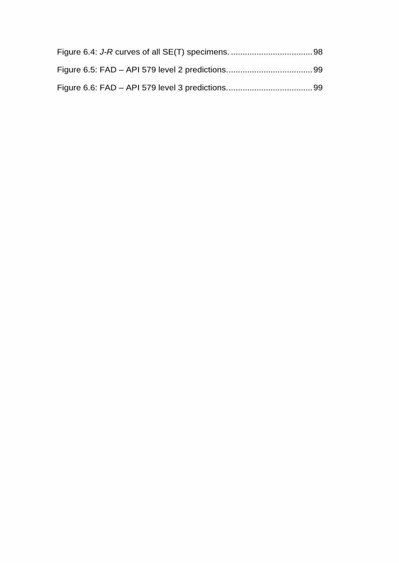
Figure 6.4: J-R curves of all SE(T) specimens. ................................... 98

Figure 6.5: FAD – API 579 level 2 predictions. .................................... 99

Figure 6.6: FAD – API 579 level 3 predictions. .................................... 99

DBD


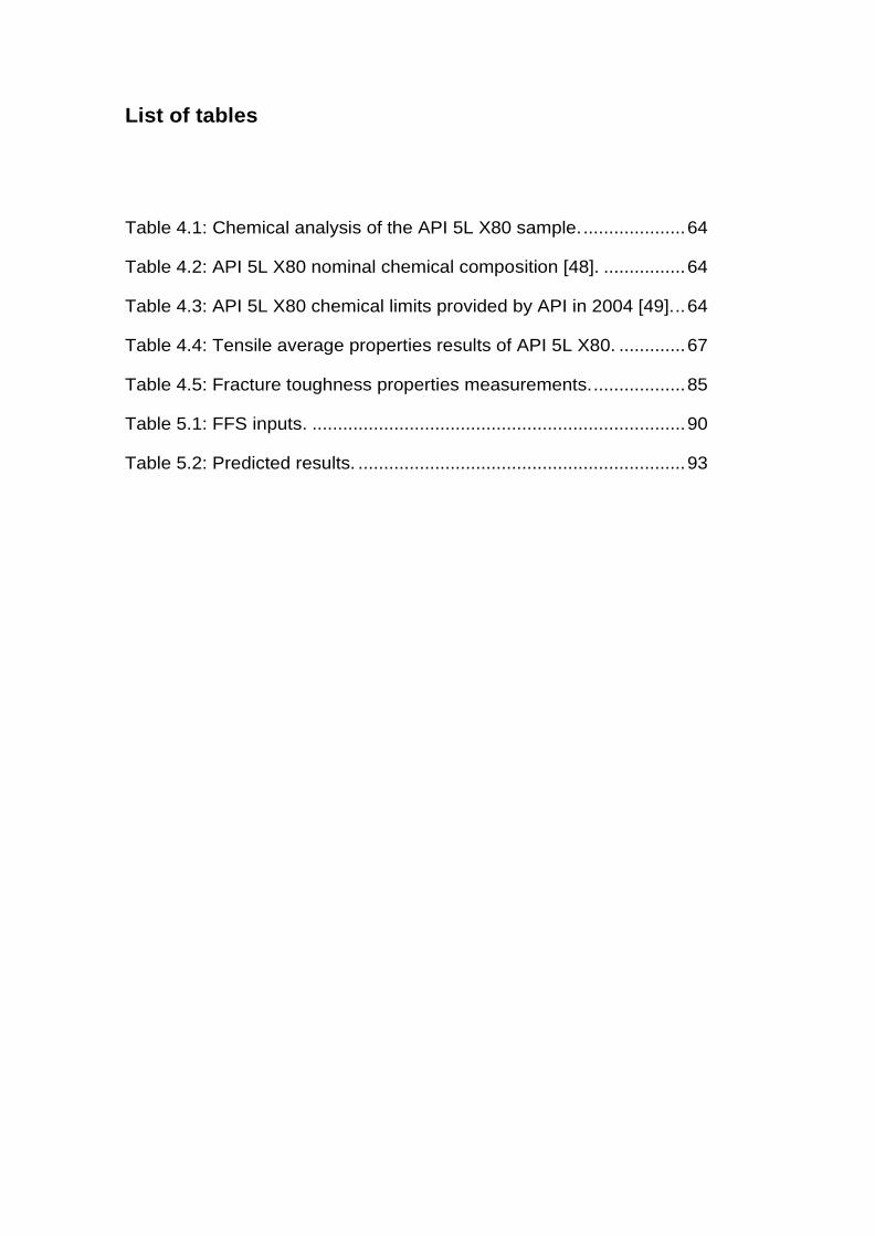
List of tables

Table 4.1: Chemical analysis of the API 5L X80 sample. .................... 64

Table 4.2: API 5L X80 nominal chemical composition [48]. ................ 64

Table 4.3: API 5L X80 chemical limits provided by API in 2004 [49]. .. 64

Table 4.4: Tensile average properties results of API 5L X80. ............. 67

Table 4.5: Fracture toughness properties measurements. .................. 85

Table 5.1: FFS inputs. ......................................................................... 90

Table 5.2: Predicted results. ................................................................ 93

DBD


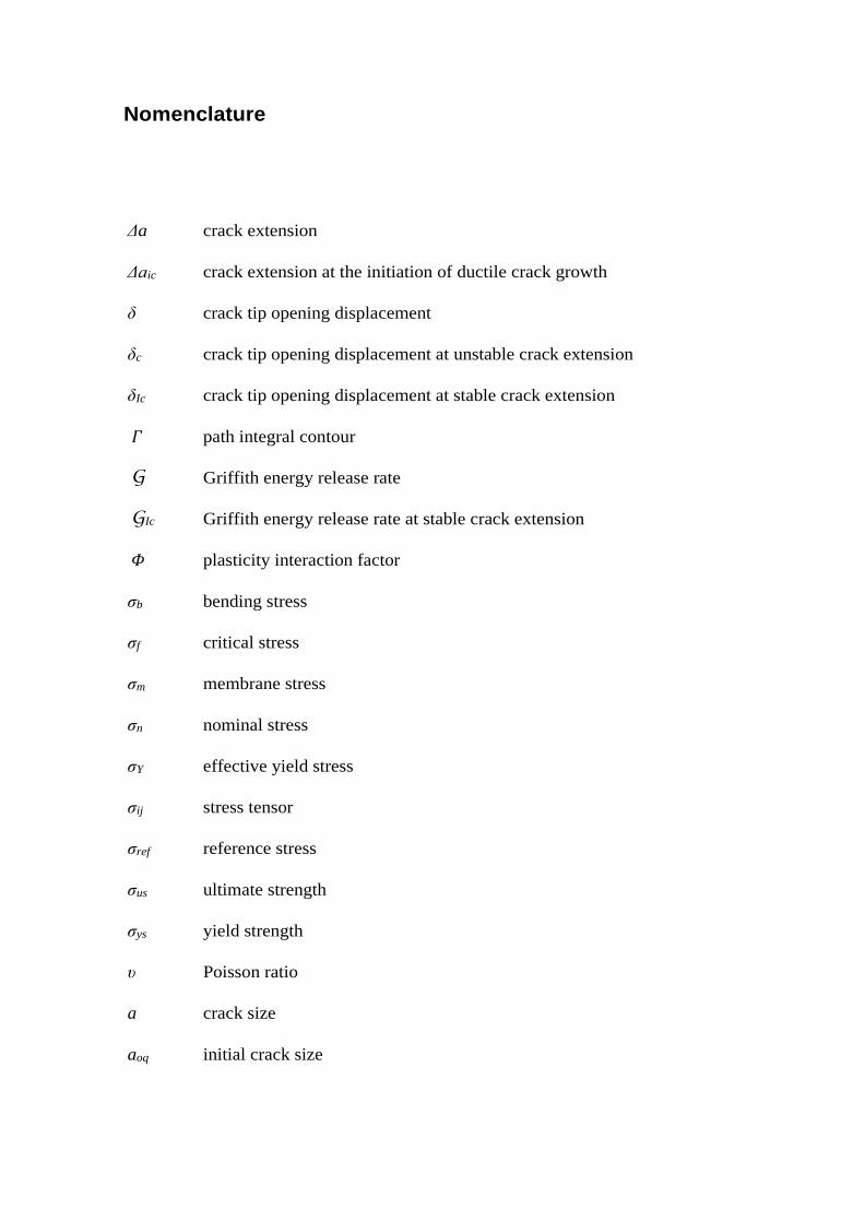
Nomenclature

Δa crack extension

Δaic crack extension at the initiation of ductile crack growth

δ crack tip opening displacement

δc crack tip opening displacement at unstable crack extension

δIc crack tip opening displacement at stable crack extension

𝛤 path integral contour

G Griffith energy release rate

GIc Griffith energy release rate at stable crack extension

𝛷 plasticity interaction factor

σb bending stress

σf critical stress

σm membrane stress

σn nominal stress

σY effective yield stress

σij stress tensor

σref reference stress

σus ultimate strength

σys yield strength

υ Poisson ratio

a crack size

aoq initial crack size

DBD


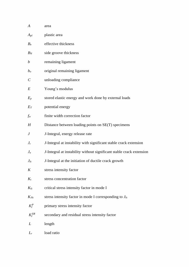
A area

Apl plastic area

Be effective thickness

BN side groove thickness

b remaining ligament

bo original remaining ligament

C unloading compliance

E Young’s modulus

Ep stored elastic energy and work done by external loads

ET potential energy

fw finite width correction factor

H Distance between loading points on SE(T) specimens

J J-Integral, energy release rate

Jc J-Integral at instability with significant stable crack extension

Ju J-Integral at instability without significant stable crack extension

JIc J-Integral at the initiation of ductile crack growth

K stress intensity factor

Kt stress concentration factor

KIc critical stress intensity factor in mode I

KJIc stress intensity factor in mode I corresponding to JIc

𝐾𝐼𝑃 primary stress intensity factor

𝐾𝐼𝑆𝑅 secondary and residual stress intensity factor

L length

Lr load ratio

DBD


P load

Pm maximum fatigue load

PY effective yield load

R fatigue load ratio

𝑟 radius

S support span

Ti component traction vector

U strain energy density

u normalized unloading compliance

ui displacement vector components

W width

Ws energy required to create new crack surface

DBD


Chapter 1:

Introduction

1.

Introduction

Engineering structures can fail under service loads due to damage caused

by several mechanisms such as corrosion, creep, fatigue, plastic collapse, and/or

fracture. The consequences of such structural failures can be catastrophic, with

the loss of significant amounts of money, and sometimes even of lives. Most of

these failures are caused or much affected by cracks, which can grow until they

break the component unless properly repaired in due time. Hence, to prevent

structural failures, it is essential to analyze crack effects by understanding the

concepts of Fracture Mechanics and by using them to answer the following

questions [1].

- What is the critical crack size?

- How long does it take to reach the critical size?

- What is the residual strength of the structure as a function of the crack

size?

- Will crack growth stop?

- What is the proper inspection frequency?

- What is the admissible initial flaw size the structure can safely tolerate

at the start of its service life?

Fracture Mechanics is the field of study that deals with the effects of cracks

on fracture behavior of a given structure. Such effects depend on stress levels,

crack sizes, and material properties, as well as on the mechanism(s) that drive

the fracture [2]. It is divided into two domains, Linear Elastic Fracture

Mechanics (LEFM), suitable for modeling brittle fractures. And Elastoplastic

Fracture Mechanics (EPFM), needed to model ductile structural components.

The main difference between these groups is the relative size of the plastic zone

in front of the crack tip. If the plastic zone has a negligible size in relation to

the component's dimensions, it is possible to use LEFM concepts. Otherwise,

DBD


Chapter 1: 20

Introduction

it is necessary to use EPFM procedures. Moreover, if the plastic zone runs

through the entire residual ligament of the component, the failure mechanism is

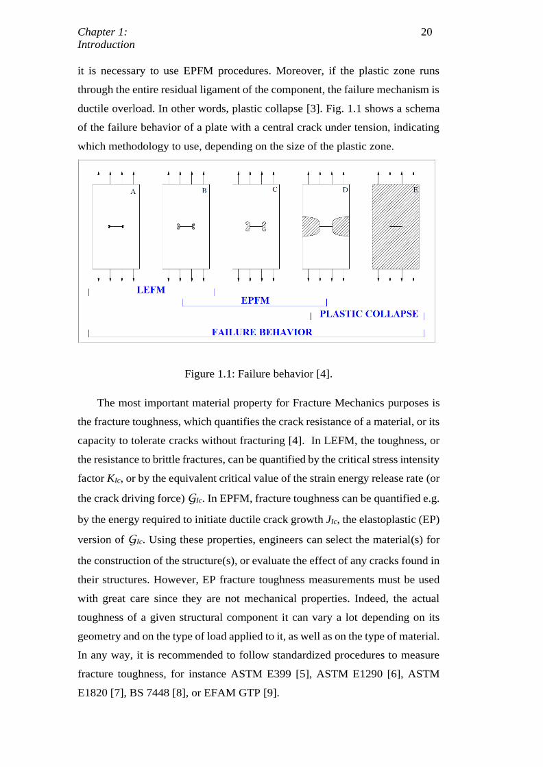
ductile overload. In other words, plastic collapse [3]. Fig. 1.1 shows a schema

of the failure behavior of a plate with a central crack under tension, indicating

which methodology to use, depending on the size of the plastic zone.

Figure 1.1: Failure behavior [4].

The most important material property for Fracture Mechanics purposes is

the fracture toughness, which quantifies the crack resistance of a material, or its

capacity to tolerate cracks without fracturing [4]. In LEFM, the toughness, or

the resistance to brittle fractures, can be quantified by the critical stress intensity

factor KIc, or by the equivalent critical value of the strain energy release rate (or

the crack driving force) GIc. In EPFM, fracture toughness can be quantified e.g.

by the energy required to initiate ductile crack growth JIc, the elastoplastic (EP)

version of GIc. Using these properties, engineers can select the material(s) for

the construction of the structure(s), or evaluate the effect of any cracks found in

their structures. However, EP fracture toughness measurements must be used

with great care since they are not mechanical properties. Indeed, the actual

toughness of a given structural component it can vary a lot depending on its

geometry and on the type of load applied to it, as well as on the type of material.

In any way, it is recommended to follow standardized procedures to measure

fracture toughness, for instance ASTM E399 [5], ASTM E1290 [6], ASTM

E1820 [7], BS 7448 [8], or EFAM GTP [9].

DBD


Chapter 1: 21

Introduction

The American Society for Testing and Materials (ASTM) issued its E1820

standard to provide normalized procedures to measure fracture toughness both

in LEFM and EPFM conditions. Among these procedures, it is possible to

measure the linear-elastic parameter KIc, and the elastoplastic parameters JIc, Ju,

Jc, δc, J-R and δ-R curves based on SE(B), C(T), and DC(T) specimens [10].

The basic procedure for measuring JIc requires multiple specimens to evaluate

a single parameter. Another procedure uses the elastic compliance technique

that can generate an entire J-resistance or J-R curve from unloading/reloading

sequences during the fracturing process (see chapter 3.1.2). This procedure

deserves attention, because it uses a single specimen on the test, resulting in a

significant economy of time and material.

The SE(B), C(T), and DC(T) specimens recommended by the standard are

highly constrained. In other words, they inhibit plastic deformation in front of

the crack tip, due to the highly triaxial stress state acting there. Hence, they

guarantee or tend to characterize plane strain conditions around the crack tip.

Because of that, a material that in theory is ductile may present a more brittle

behavior in that region, resulting in lower values of its measured fracture

toughness, a safety requirement for most structural design applications.

However, some engineering structures such as pipelines and pressure vessels

work under much lower constraint conditions, making the standard

conservative, but also leading to uneconomic designs. With this in mind, the

clamped SE(T) specimen provides more similar constraints conditions when

compared with pipelines and pressure vessels [11]. This specimen generally

develops lower stress triaxiality in front of the crack tip when compared to

SE(B), C(T), and DC(T) specimens.

It is basically impossible to claim that structures do not have any flaw,

especially when they work under variable loadings in long-term operations.

Therefore, it is necessary to check if the structure can operate under the presence

of any flaw. For that reason, groups of engineers came together to develop

accurate assessments of Structural Integrity for safety analysis of engineering

structures, which include pipelines and pressure vessels, for example. The

American Petroleum Institute (API) developed its API-579 Fitness-For-Service

(FFS) guide [12], which recommends engineering procedures for structural

DBD


Chapter 1: 22

Introduction

integrity evaluations on the petrochemical industry. The primary objective of

the FFS assessment is to prevent failures. There are other similar standards like

the R6 [13], SAQ [14], SINTAP [15], and BS7910 [16], which also issue

recommended procedures to evaluate crack effects in structures. Chapter 1.1

shows some examples of disasters caused by cracks in real life.

1.1

Disasters

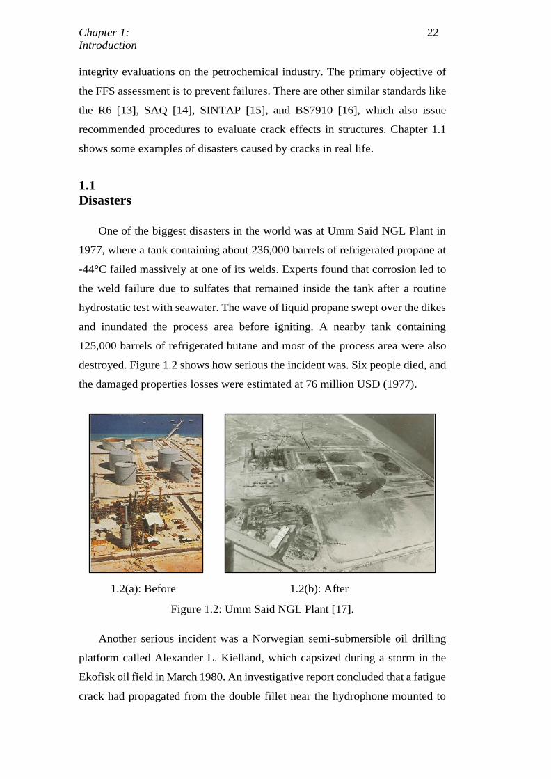
One of the biggest disasters in the world was at Umm Said NGL Plant in

1977, where a tank containing about 236,000 barrels of refrigerated propane at

-44°C failed massively at one of its welds. Experts found that corrosion led to

the weld failure due to sulfates that remained inside the tank after a routine

hydrostatic test with seawater. The wave of liquid propane swept over the dikes

and inundated the process area before igniting. A nearby tank containing

125,000 barrels of refrigerated butane and most of the process area were also

destroyed. Figure 1.2 shows how serious the incident was. Six people died, and

the damaged properties losses were estimated at 76 million USD (1977).

Figure 1.2: Umm Said NGL Plant [17].

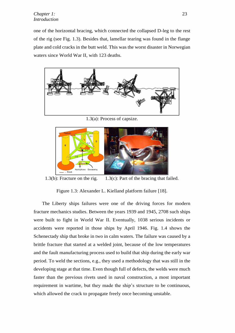
Another serious incident was a Norwegian semi-submersible oil drilling

platform called Alexander L. Kielland, which capsized during a storm in the

Ekofisk oil field in March 1980. An investigative report concluded that a fatigue

crack had propagated from the double fillet near the hydrophone mounted to

1.2(a): Before 1.2(b): After

DBD


Chapter 1: 23

Introduction

one of the horizontal bracing, which connected the collapsed D-leg to the rest

of the rig (see Fig. 1.3). Besides that, lamellar tearing was found in the flange

plate and cold cracks in the butt weld. This was the worst disaster in Norwegian

waters since World War II, with 123 deaths.

1.3(a): Process of capsize.

1.3(b): Fracture on the rig. 1.3(c): Part of the bracing that failed.

Figure 1.3: Alexander L. Kielland platform failure [18].

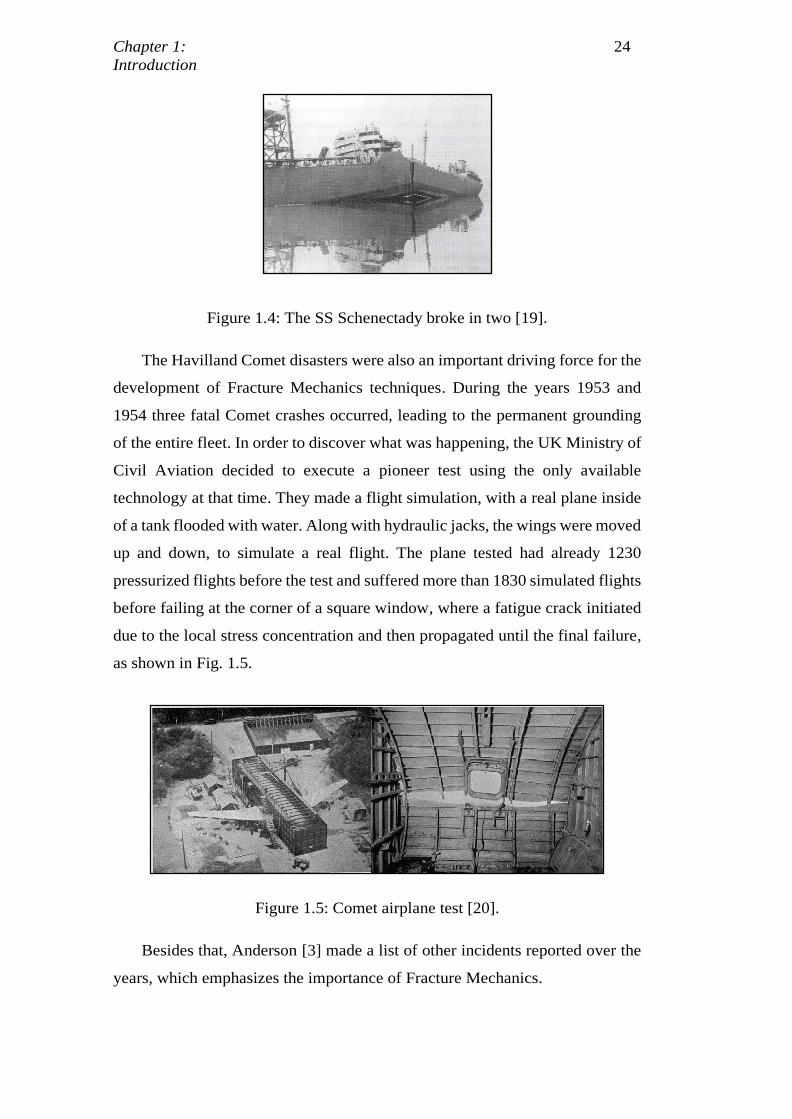
The Liberty ships failures were one of the driving forces for modern

fracture mechanics studies. Between the years 1939 and 1945, 2708 such ships

were built to fight in World War II. Eventually, 1038 serious incidents or

accidents were reported in those ships by April 1946. Fig. 1.4 shows the

Schenectady ship that broke in two in calm waters. The failure was caused by a

brittle fracture that started at a welded joint, because of the low temperatures

and the fault manufacturing process used to build that ship during the early war

period. To weld the sections, e.g., they used a methodology that was still in the

developing stage at that time. Even though full of defects, the welds were much

faster than the previous rivets used in naval construction, a most important

requirement in wartime, but they made the ship’s structure to be continuous,

which allowed the crack to propagate freely once becoming unstable.

DBD


Chapter 1: 24

Introduction

Figure 1.4: The SS Schenectady broke in two [19].

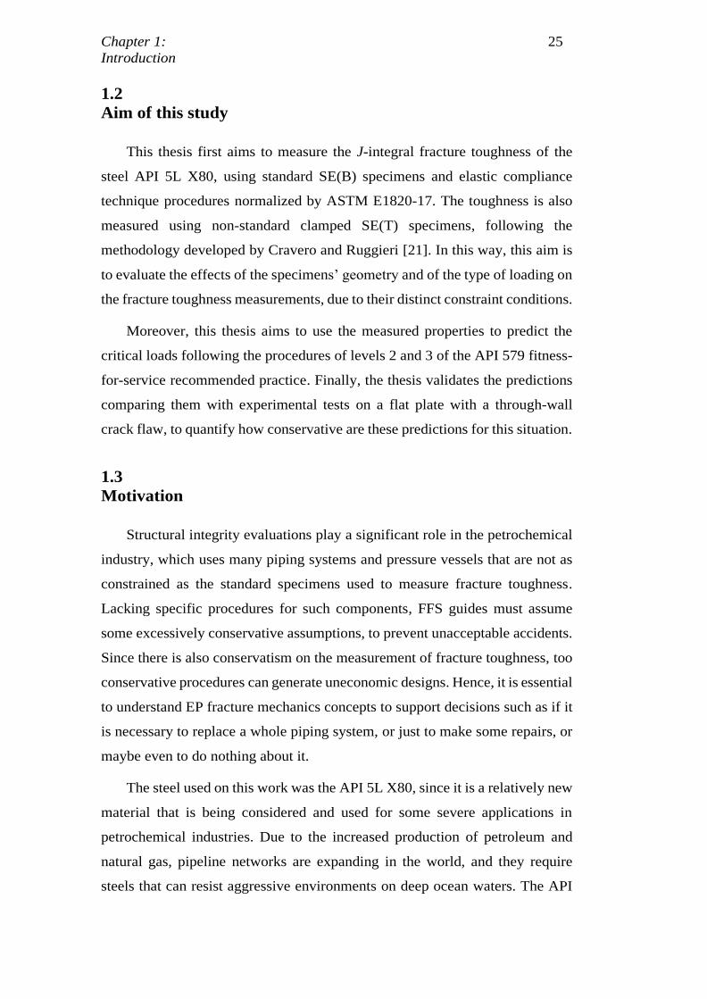
The Havilland Comet disasters were also an important driving force for the

development of Fracture Mechanics techniques. During the years 1953 and

1954 three fatal Comet crashes occurred, leading to the permanent grounding

of the entire fleet. In order to discover what was happening, the UK Ministry of

Civil Aviation decided to execute a pioneer test using the only available

technology at that time. They made a flight simulation, with a real plane inside

of a tank flooded with water. Along with hydraulic jacks, the wings were moved

up and down, to simulate a real flight. The plane tested had already 1230

pressurized flights before the test and suffered more than 1830 simulated flights

before failing at the corner of a square window, where a fatigue crack initiated

due to the local stress concentration and then propagated until the final failure,

as shown in Fig. 1.5.

Figure 1.5: Comet airplane test [20].

Besides that, Anderson [3] made a list of other incidents reported over the

years, which emphasizes the importance of Fracture Mechanics.

DBD


Chapter 1: 25

Introduction

1.2

Aim of this study

This thesis first aims to measure the J-integral fracture toughness of the

steel API 5L X80, using standard SE(B) specimens and elastic compliance

technique procedures normalized by ASTM E1820-17. The toughness is also

measured using non-standard clamped SE(T) specimens, following the

methodology developed by Cravero and Ruggieri [21]. In this way, this aim is

to evaluate the effects of the specimens’ geometry and of the type of loading on

the fracture toughness measurements, due to their distinct constraint conditions.

Moreover, this thesis aims to use the measured properties to predict the

critical loads following the procedures of levels 2 and 3 of the API 579 fitness-

for-service recommended practice. Finally, the thesis validates the predictions

comparing them with experimental tests on a flat plate with a through-wall

crack flaw, to quantify how conservative are these predictions for this situation.

1.3

Motivation

Structural integrity evaluations play a significant role in the petrochemical

industry, which uses many piping systems and pressure vessels that are not as

constrained as the standard specimens used to measure fracture toughness.

Lacking specific procedures for such components, FFS guides must assume

some excessively conservative assumptions, to prevent unacceptable accidents.

Since there is also conservatism on the measurement of fracture toughness, too

conservative procedures can generate uneconomic designs. Hence, it is essential

to understand EP fracture mechanics concepts to support decisions such as if it

is necessary to replace a whole piping system, or just to make some repairs, or

maybe even to do nothing about it.

The steel used on this work was the API 5L X80, since it is a relatively new

material that is being considered and used for some severe applications in

petrochemical industries. Due to the increased production of petroleum and

natural gas, pipeline networks are expanding in the world, and they require

steels that can resist aggressive environments on deep ocean waters. The API

DBD


Chapter 1: 26

Introduction

5L X80 is a dual-phase High Strength and Low Alloy (HSLA) steel, a class of

materials that have been developed to support such requirements. They allow

the reduction of pipeline thicknesses, resulting in weight reduction and lower

consumption of raw material. Moreover, the API 5L X80 has good weldability

and low hardenability. The microstructure is composed of acicular ferrite with

a small amount of martensite/austenite, that results in high tensile strength and

low ductile to brittle transition temperature. The steel is manufactured with a

controlled lamination process, which refines the grains and precipitates carbides

and nitrides of the micro-alloyed elements. Because of that, it prevents

recrystallization, causing their strength resistance increase without adding

carbon or manganese in the alloy. As a result, it hinders the toughness and

weldability of the material [22] [23]. These types of steels manufactured for

pipeline systems are classified according to the American Petroleum Institute

(API). The grade X80 means that the steel has a yield strength of at least 80 ksi

or 550MPa.

1.4

Thesis structure

Chapter 1, resumes the importance of this subject, presents the aims of this

study, and review the motivations for this work.

Chapter 2 reviews some basic Fracture Mechanics concepts and properties

definitions.

Chapter 3 reviews procedures to measure fracture toughness using SE(B)

and SE(T) specimens.

Chapter 4 lists the results of the material's properties measurements.

Chapter 5 studies structural integrity procedures proposed in API 579, and

presents predictions and experimental tests for the case in question here.

Chapter 6 summarizes all the experimental results obtained in this work.

Chapter 7 presents the conclusions and address future work suggestions.

DBD


Chapter 2:

Theoretical background

2.


This chapter introduces the terminology used in this work and briefly

reviews. As well some mechanical property definitions and basic concepts of

Fracture Mechanics pertinent to its purposes.

2.1

Tensile strength and ductility

Steels, like most structural metallic alloys, obey a linear relationship

between stresses and strains while they remain elastic following Hooke’s law

until they reach their proportional limit, after which plastic strains are induced

in them. Young's modulus (E) defines the ratio between LE stresses and strains,

which quantifies the material stiffness. After the proportional limit, the material

yields and start to accumulate plastic strains.

Ductility is the capacity to tolerate plastic strains, and it can be measured

by the residual elongation of a base of measurement marked on the specimen

surface before the tensile test. Or else, by the reduction in the area of the necked

section after the test.

Since the proportional limit is difficult to measure, engineers use the Yield

Strength (σys), which defines the stress required to cause an arbitrary small

amount of plastic deformation on standard tensile specimens of the material.

ASTM E8/E8M [24] defines σys by the intersection of the stress-strain curve

with a 0.2% offset line parallel to its linear zone. Hence, the yield strength

should not be confused with the proportional limit of the material. Indeed, a

stress = ys leaves a residual plastic strain pl = 0.2% after unloading the

tensile specimen.

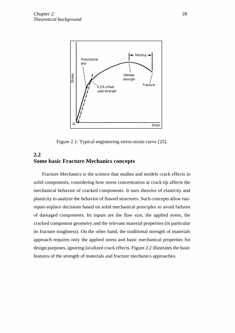
Looking at the engineering stress-strain curve (Fig. 2.1), the Ultimate

Strength (σus) is the highest stress the material can support before breaking, or

the stress required to start the necking in a tension test. After that point, the

engineering stress decreases until the fracture occurs.

DBD


Chapter 2: 28


Figure 2.1: Typical engineering stress-strain curve [25].

2.2

Some basic Fracture Mechanics concepts

Fracture Mechanics is the science that studies and models crack effects in

solid components, considering how stress concentration at crack tip affects the

mechanical behavior of cracked components. It uses theories of elasticity and

plasticity to analyze the behavior of flawed structures. Such concepts allow run-

repair-replace decisions based on solid mechanical principles to avoid failures

of damaged components. Its inputs are the flaw size, the applied stress, the

cracked component geometry and the relevant material properties (in particular

its fracture toughness). On the other hand, the traditional strength of materials

approach requires only the applied stress and basic mechanical properties for

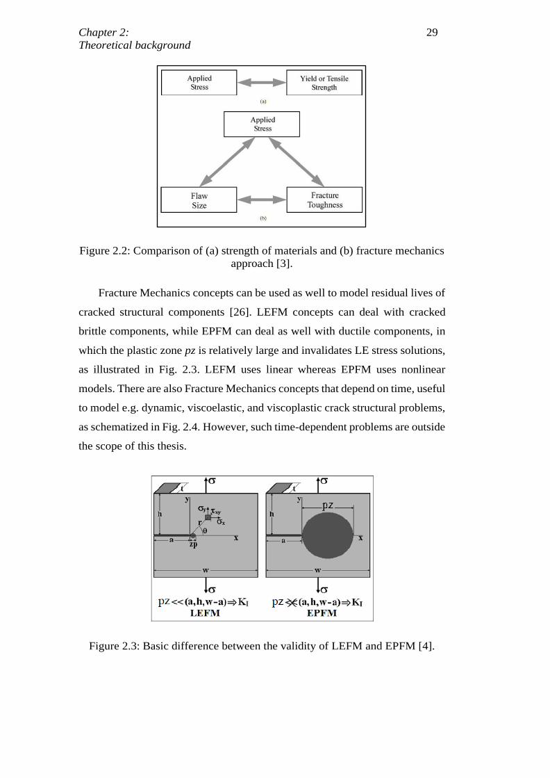
design purposes, ignoring localized crack effects. Figure 2.2 illustrates the basic

features of the strength of materials and fracture mechanics approaches.

DBD


Chapter 2: 29


Figure 2.2: Comparison of (a) strength of materials and (b) fracture mechanics

approach [3].

Fracture Mechanics concepts can be used as well to model residual lives of

cracked structural components [26]. LEFM concepts can deal with cracked

brittle components, while EPFM can deal as well with ductile components, in

which the plastic zone pz is relatively large and invalidates LE stress solutions,

as illustrated in Fig. 2.3. LEFM uses linear whereas EPFM uses nonlinear

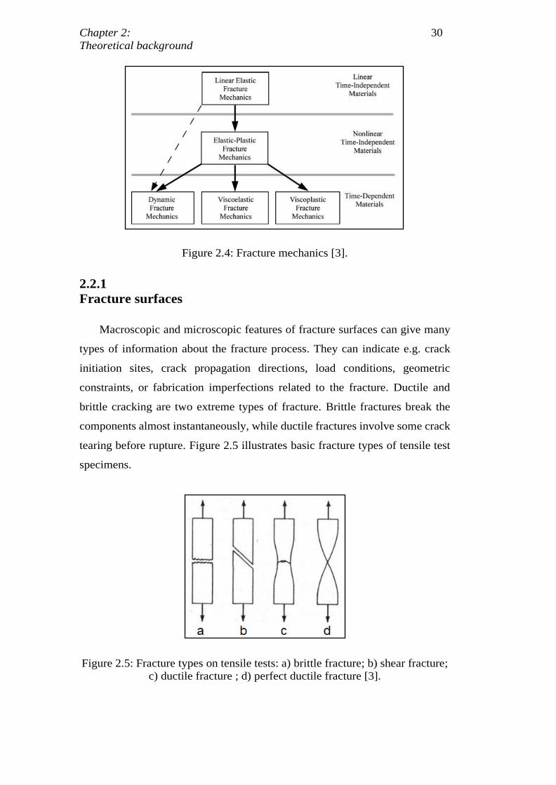
models. There are also Fracture Mechanics concepts that depend on time, useful

to model e.g. dynamic, viscoelastic, and viscoplastic crack structural problems,

as schematized in Fig. 2.4. However, such time-dependent problems are outside

the scope of this thesis.

Figure 2.3: Basic difference between the validity of LEFM and EPFM [4].

DBD


Chapter 2: 30


Figure 2.4: Fracture mechanics [3].

2.2.1

Fracture surfaces

Macroscopic and microscopic features of fracture surfaces can give many

types of information about the fracture process. They can indicate e.g. crack

initiation sites, crack propagation directions, load conditions, geometric

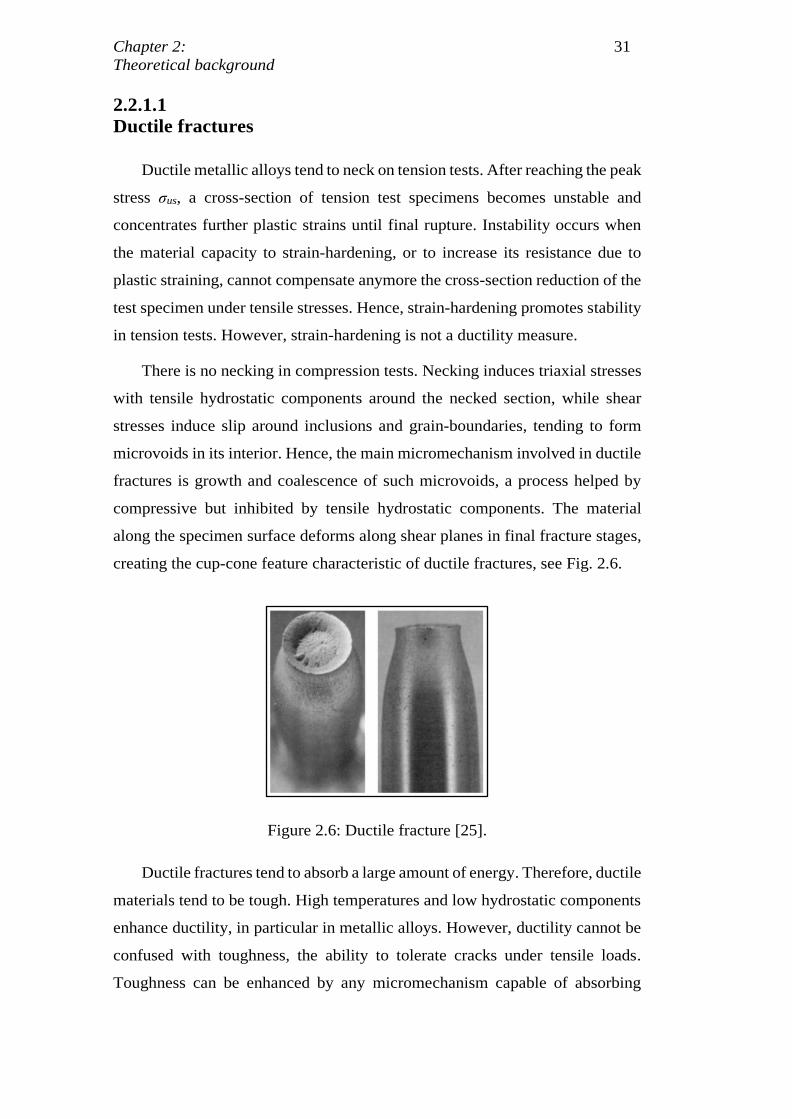
constraints, or fabrication imperfections related to the fracture. Ductile and

brittle cracking are two extreme types of fracture. Brittle fractures break the

components almost instantaneously, while ductile fractures involve some crack

tearing before rupture. Figure 2.5 illustrates basic fracture types of tensile test

specimens.

Figure 2.5: Fracture types on tensile tests: a) brittle fracture; b) shear fracture;

c) ductile fracture ; d) perfect ductile fracture [3].

DBD


Chapter 2: 31


2.2.1.1

Ductile fractures

Ductile metallic alloys tend to neck on tension tests. After reaching the peak

stress σus, a cross-section of tension test specimens becomes unstable and

concentrates further plastic strains until final rupture. Instability occurs when

the material capacity to strain-hardening, or to increase its resistance due to

plastic straining, cannot compensate anymore the cross-section reduction of the

test specimen under tensile stresses. Hence, strain-hardening promotes stability

in tension tests. However, strain-hardening is not a ductility measure.

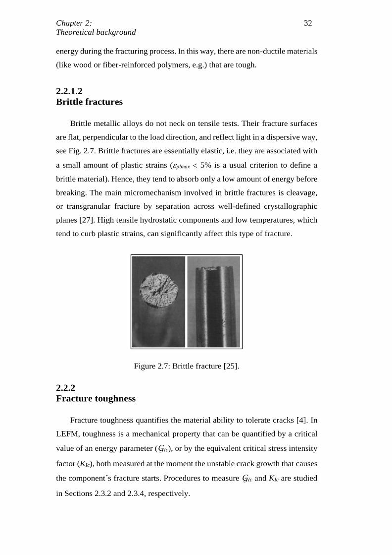
There is no necking in compression tests. Necking induces triaxial stresses

with tensile hydrostatic components around the necked section, while shear

stresses induce slip around inclusions and grain-boundaries, tending to form

microvoids in its interior. Hence, the main micromechanism involved in ductile

fractures is growth and coalescence of such microvoids, a process helped by

compressive but inhibited by tensile hydrostatic components. The material

along the specimen surface deforms along shear planes in final fracture stages,

creating the cup-cone feature characteristic of ductile fractures, see Fig. 2.6.

Figure 2.6: Ductile fracture [25].

Ductile fractures tend to absorb a large amount of energy. Therefore, ductile

materials tend to be tough. High temperatures and low hydrostatic components

enhance ductility, in particular in metallic alloys. However, ductility cannot be

confused with toughness, the ability to tolerate cracks under tensile loads.

Toughness can be enhanced by any micromechanism capable of absorbing

DBD


Chapter 2: 32


energy during the fracturing process. In this way, there are non-ductile materials

(like wood or fiber-reinforced polymers, e.g.) that are tough.

2.2.1.2

Brittle fractures

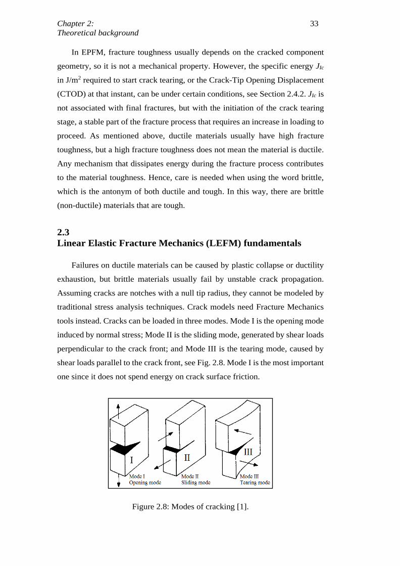
Brittle metallic alloys do not neck on tensile tests. Their fracture surfaces

are flat, perpendicular to the load direction, and reflect light in a dispersive way,

see Fig. 2.7. Brittle fractures are essentially elastic, i.e. they are associated with

a small amount of plastic strains (plmax 5% is a usual criterion to define a

brittle material). Hence, they tend to absorb only a low amount of energy before

breaking. The main micromechanism involved in brittle fractures is cleavage,

or transgranular fracture by separation across well-defined crystallographic

planes [27]. High tensile hydrostatic components and low temperatures, which

tend to curb plastic strains, can significantly affect this type of fracture.

Figure 2.7: Brittle fracture [25].

2.2.2

Fracture toughness

Fracture toughness quantifies the material ability to tolerate cracks [4]. In

LEFM, toughness is a mechanical property that can be quantified by a critical

value of an energy parameter (GIc), or by the equivalent critical stress intensity

factor (KIc), both measured at the moment the unstable crack growth that causes

the component´s fracture starts. Procedures to measure GIc and KIc are studied

in Sections 2.3.2 and 2.3.4, respectively.

DBD


Chapter 2: 33


In EPFM, fracture toughness usually depends on the cracked component

geometry, so it is not a mechanical property. However, the specific energy JIc

in J/m2 required to start crack tearing, or the Crack-Tip Opening Displacement

(CTOD) at that instant, can be under certain conditions, see Section 2.4.2. JIc is

not associated with final fractures, but with the initiation of the crack tearing

stage, a stable part of the fracture process that requires an increase in loading to

proceed. As mentioned above, ductile materials usually have high fracture

toughness, but a high fracture toughness does not mean the material is ductile.

Any mechanism that dissipates energy during the fracture process contributes

to the material toughness. Hence, care is needed when using the word brittle,

which is the antonym of both ductile and tough. In this way, there are brittle

(non-ductile) materials that are tough.

2.3

Linear Elastic Fracture Mechanics (LEFM) fundamentals

Failures on ductile materials can be caused by plastic collapse or ductility

exhaustion, but brittle materials usually fail by unstable crack propagation.

Assuming cracks are notches with a null tip radius, they cannot be modeled by

traditional stress analysis techniques. Crack models need Fracture Mechanics

tools instead. Cracks can be loaded in three modes. Mode I is the opening mode

induced by normal stress; Mode II is the sliding mode, generated by shear loads

perpendicular to the crack front; and Mode III is the tearing mode, caused by

shear loads parallel to the crack front, see Fig. 2.8. Mode I is the most important

one since it does not spend energy on crack surface friction.

Figure 2.8: Modes of cracking [1].

DBD


Chapter 2: 34


2.3.1

Stress concentration factor Kt

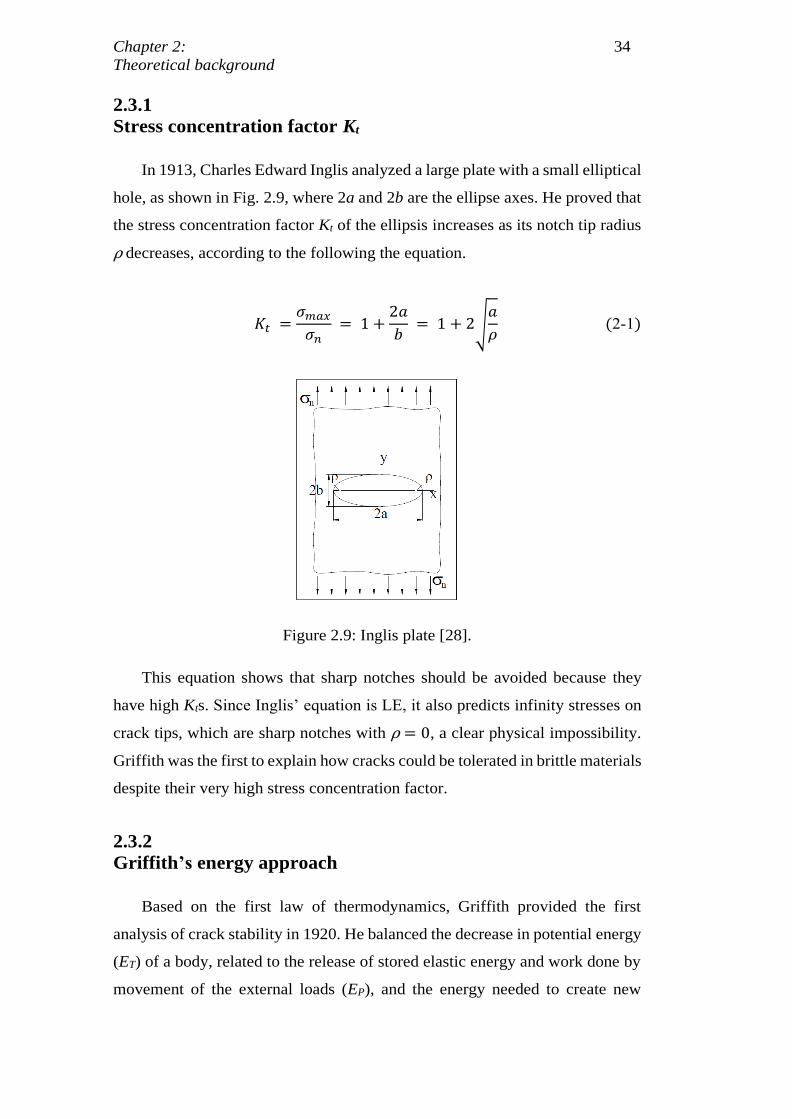
In 1913, Charles Edward Inglis analyzed a large plate with a small elliptical

hole, as shown in Fig. 2.9, where 2a and 2b are the ellipse axes. He proved that

the stress concentration factor Kt of the ellipsis increases as its notch tip radius

ρ decreases, according to the following the equation.

𝐾𝑡 =𝜎𝑚𝑎𝑥

𝜎𝑛 = 1 +

2𝑎

𝑏 = 1 + 2√

𝑎

𝜌(2-1)

Figure 2.9: Inglis plate [28].

This equation shows that sharp notches should be avoided because they

have high Kts. Since Inglis’ equation is LE, it also predicts infinity stresses on

crack tips, which are sharp notches with ρ = 0, a clear physical impossibility.

Griffith was the first to explain how cracks could be tolerated in brittle materials

despite their very high stress concentration factor.

2.3.2

Griffith’s energy approach

Based on the first law of thermodynamics, Griffith provided the first

analysis of crack stability in 1920. He balanced the decrease in potential energy

(ET) of a body, related to the release of stored elastic energy and work done by

movement of the external loads (EP), and the energy needed to create new

DBD


Chapter 2: 35


surfaces (Ws), due to the crack propagation in ideally brittle materials. Griffith

energy balance under static conditions, for an incremental increase in crack area

dA, can be expressed in the following way:

𝑑𝐸𝑇

𝑑𝐴=

𝑑𝐸𝑝

𝑑𝐴+

𝑑𝑊𝑠

𝑑𝐴= 0 (2-2)

Brittle fracture occurs when the strain energy released rate associated with

crack extension is larger than the energy spent to create new crack surfaces.

Based on the analysis developed by Inglis, the potential energy of the plate with

an elliptic hole is given by:

𝐸𝑝 =𝜋𝜎2𝑎2𝐵

𝐸(2-3)

where E is Young's modulus, and B is the plate thickness. The energy required

to create new surfaces Ws is defined as:

𝑊𝑠 = 4𝑎𝐵𝛾𝑠 (2-4)

where 𝛾𝑠 is the specific surface energy. Rewriting Eq. 2-2, taking into account

Eq. 2-3 and 2-4, it is possible to define the critical stress (σf) for plane strain:

𝜎𝑓 = √2𝐸𝛾𝑠

𝜋𝑎(2-5)

Irwin and Orowan [4] independently modified the Griffith expression to

account for materials that are not ideally LE, taking into account the plastic

work per unit area of surface created 𝛾𝑝. They re-defined the fracture energy by

𝑤𝑓 = γ𝑠 + γ𝑝, considering elastic and plastic, viscoelastic, or viscoplastic

effects, depending on the material.

2.3.3

Energy release rate

Irwin [13] developed the modern version of Griffith’s energy approach,

defining the potential energy release rate per unit area G by:

𝒢 = −𝜕𝐸𝑝

𝜕𝐴(2-6)

DBD


Chapter 2: 36


For a wide plate with a central crack, G is given by:

𝒢 =𝜋𝜎2𝑎

𝐸(2-7)

He assumed that fracture occurs when G reaches GIc, the critical value of

the potential energy release rate, or the toughness of the material in mode I.

𝒢𝐼𝑐 =𝑑𝑊𝑠

𝑑𝐴(2-8)

2.3.4

Stress intensity factors

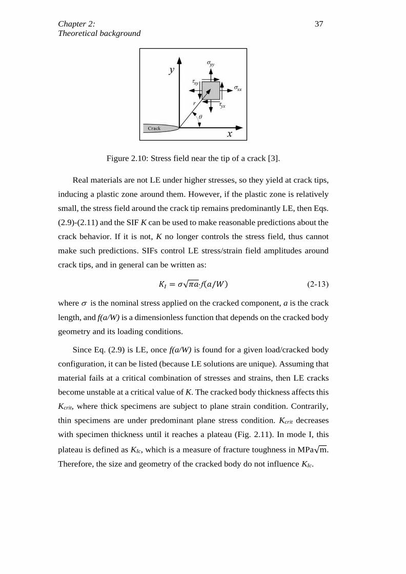
In 1957, Irwin and Williams independently analyzed 2D LE stress-strain

fields around crack tips. Considering polar coordinates with origin at the crack

tip (Fig. 2.10), the stress field in Mode I is given by

𝜎𝑖𝑗 =𝐾𝐼

√2𝜋𝑟f𝑖𝑗(𝜃) (2-9)

where σ𝑖𝑗 are the stresses, 𝑟 and 𝜃 are polar coordinates, fij() are dimensionless

functions, and KI is the Mode I Stress Intensity Factor (SIF), which depends on

the cracked body geometry and its loading conditions.

Since the stresses vary with 1/√𝑟, this equation is singular ( → when

𝑟 → 0). On the other hand, it predicts → 0 for large 𝑟, instead of the nominal

stress. Hence, this equation is valid only for a limited area around the crack tip,

and it results in:

𝜎𝑥𝑥 =𝐾𝐼

√2𝜋𝑟cos (

𝜃

2) [1 − sin (

𝜃

2) sin (

3𝜃

2)] (2-10)

𝜎𝑦𝑦 =𝐾𝐼

√2𝜋𝑟cos (

𝜃

2) [1 + sin (

𝜃

2) sin (

3𝜃

2)] (2-11)

𝜏𝑥𝑦 =𝐾𝐼

√2𝜋𝑟cos (

𝜃

2) sin (

𝜃

2) cos (

3𝜃

2) (2-12)

DBD


Chapter 2: 37


Figure 2.10: Stress field near the tip of a crack [3].

Real materials are not LE under higher stresses, so they yield at crack tips,

inducing a plastic zone around them. However, if the plastic zone is relatively

small, the stress field around the crack tip remains predominantly LE, then Eqs.

(2.9)-(2.11) and the SIF K can be used to make reasonable predictions about the

crack behavior. If it is not, K no longer controls the stress field, thus cannot

make such predictions. SIFs control LE stress/strain field amplitudes around

crack tips, and in general can be written as:

𝐾𝐼 = 𝜎√𝜋𝑎f(𝑎/𝑊) (2-13)

where is the nominal stress applied on the cracked component, a is the crack

length, and f(a/W) is a dimensionless function that depends on the cracked body

geometry and its loading conditions.

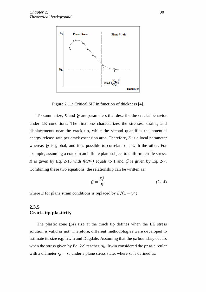
Since Eq. (2.9) is LE, once f(a/W) is found for a given load/cracked body

configuration, it can be listed (because LE solutions are unique). Assuming that

material fails at a critical combination of stresses and strains, then LE cracks

become unstable at a critical value of K. The cracked body thickness affects this

Kcrit, where thick specimens are subject to plane strain condition. Contrarily,

thin specimens are under predominant plane stress condition. Kcrit decreases

with specimen thickness until it reaches a plateau (Fig. 2.11). In mode I, this

plateau is defined as KIc, which is a measure of fracture toughness in MPa√m.

Therefore, the size and geometry of the cracked body do not influence KIc.

DBD


Chapter 2: 38


Figure 2.11: Critical SIF in function of thickness [4].

To summarize, K and G are parameters that describe the crack's behavior

under LE conditions. The first one characterizes the stresses, strains, and

displacements near the crack tip, while the second quantifies the potential

energy release rate per crack extension area. Therefore, K is a local parameter

whereas G is global, and it is possible to correlate one with the other. For

example, assuming a crack in an infinite plate subject to uniform tensile stress,

K is given by Eq. 2-13 with f(a/W) equals to 1 and G is given by Eq. 2-7.

Combining these two equations, the relationship can be written as:

𝒢 =𝐾𝐼

2

𝐸(2-14)

where E for plane strain conditions is replaced by 𝐸/(1 − υ2).

2.3.5

Crack-tip plasticity

The plastic zone (pz) size at the crack tip defines when the LE stress

solution is valid or not. Therefore, different methodologies were developed to

estimate its size e.g. Irwin and Dugdale. Assuming that the pz boundary occurs

when the stress given by Eq. 2-9 reaches ys, Irwin considered the pz as circular

with a diameter 𝑟𝑝 = 𝑟𝑦 under a plane stress state, where 𝑟𝑦 is defined as:

DBD


Chapter 2: 39


𝑟𝑦 =1

2𝜋(

𝐾𝐼

𝜎𝑦𝑠)

2

(2-15)

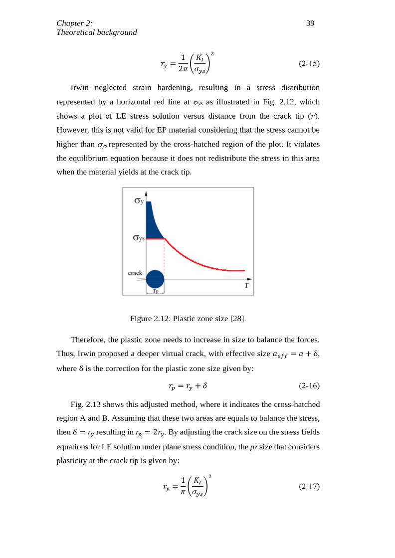
Irwin neglected strain hardening, resulting in a stress distribution

represented by a horizontal red line at ys as illustrated in Fig. 2.12, which

shows a plot of LE stress solution versus distance from the crack tip (𝑟).

However, this is not valid for EP material considering that the stress cannot be

higher than ys represented by the cross-hatched region of the plot. It violates

the equilibrium equation because it does not redistribute the stress in this area

when the material yields at the crack tip.

Figure 2.12: Plastic zone size [28].

Therefore, the plastic zone needs to increase in size to balance the forces.

Thus, Irwin proposed a deeper virtual crack, with effective size 𝑎𝑒𝑓𝑓 = 𝑎 + δ,

where δ is the correction for the plastic zone size given by:

𝑟𝑝 = 𝑟𝑦 + 𝛿 (2-16)

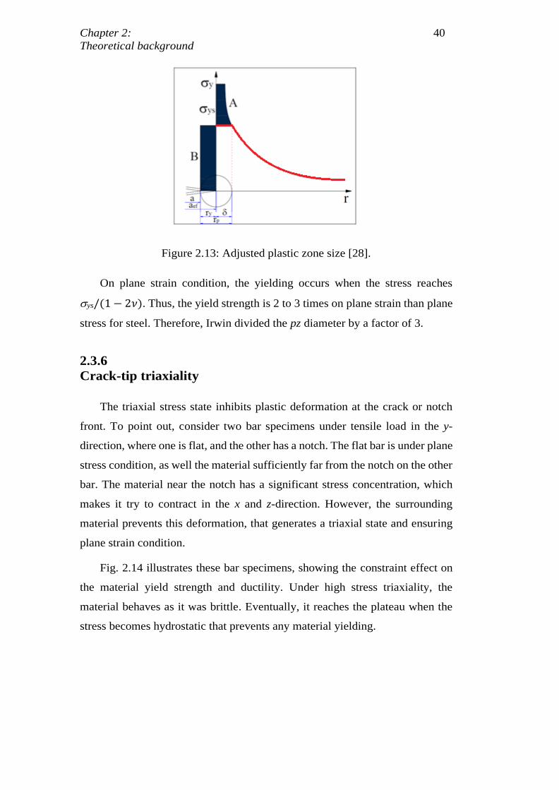
Fig. 2.13 shows this adjusted method, where it indicates the cross-hatched

region A and B. Assuming that these two areas are equals to balance the stress,

then δ = 𝑟𝑦 resulting in 𝑟𝑝 = 2𝑟𝑦. By adjusting the crack size on the stress fields

equations for LE solution under plane stress condition, the pz size that considers

plasticity at the crack tip is given by:

𝑟𝑦 =1

𝜋(

𝐾𝐼

𝜎𝑦𝑠)

2

(2-17)

DBD


Chapter 2: 40


Figure 2.13: Adjusted plastic zone size [28].

On plane strain condition, the yielding occurs when the stress reaches

ys/(1 − 2𝜈). Thus, the yield strength is 2 to 3 times on plane strain than plane

stress for steel. Therefore, Irwin divided the pz diameter by a factor of 3.

2.3.6

Crack-tip triaxiality

The triaxial stress state inhibits plastic deformation at the crack or notch

front. To point out, consider two bar specimens under tensile load in the y-

direction, where one is flat, and the other has a notch. The flat bar is under plane

stress condition, as well the material sufficiently far from the notch on the other

bar. The material near the notch has a significant stress concentration, which

makes it try to contract in the x and z-direction. However, the surrounding

material prevents this deformation, that generates a triaxial state and ensuring

plane strain condition.

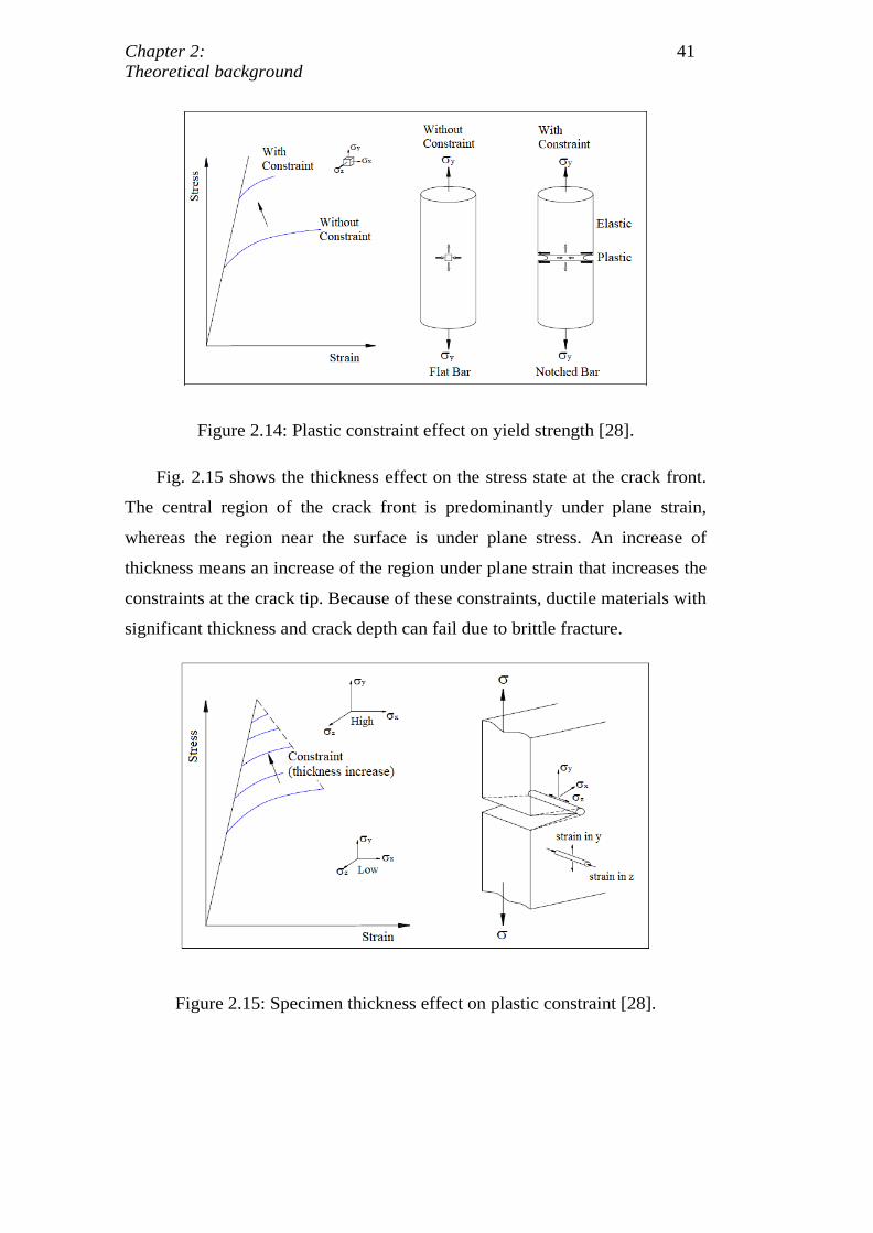
Fig. 2.14 illustrates these bar specimens, showing the constraint effect on

the material yield strength and ductility. Under high stress triaxiality, the

material behaves as it was brittle. Eventually, it reaches the plateau when the

stress becomes hydrostatic that prevents any material yielding.

DBD


Chapter 2: 41


Figure 2.14: Plastic constraint effect on yield strength [28].

Fig. 2.15 shows the thickness effect on the stress state at the crack front.

The central region of the crack front is predominantly under plane strain,

whereas the region near the surface is under plane stress. An increase of

thickness means an increase of the region under plane strain that increases the

constraints at the crack tip. Because of these constraints, ductile materials with

significant thickness and crack depth can fail due to brittle fracture.

Figure 2.15: Specimen thickness effect on plastic constraint [28].

DBD


Chapter 2: 42


2.4

Elastic-Plastic Fracture Mechanics (EPFM) fundamentals

Elastic-plastic fracture mechanics extends the studies of fracture behavior

beyond the LE regime. The EPFM applies to materials that have a significant

plastic deformation, resulting in a nonlinear elastic region at the crack-tip. The

two main parameters are the Crack Tip Opening Displacement (CTOD) and the

J contour integral. Both describe crack-tip conditions in EP materials and have

critical values that can be used to quantify fracture toughness under moderate-

to-high crack tip plasticity. The EPFM also has a limitation, since it does not

treat the occurrence of plastic collapse.

2.4.1

Crack-Tip Opening Displacement (CTOD)

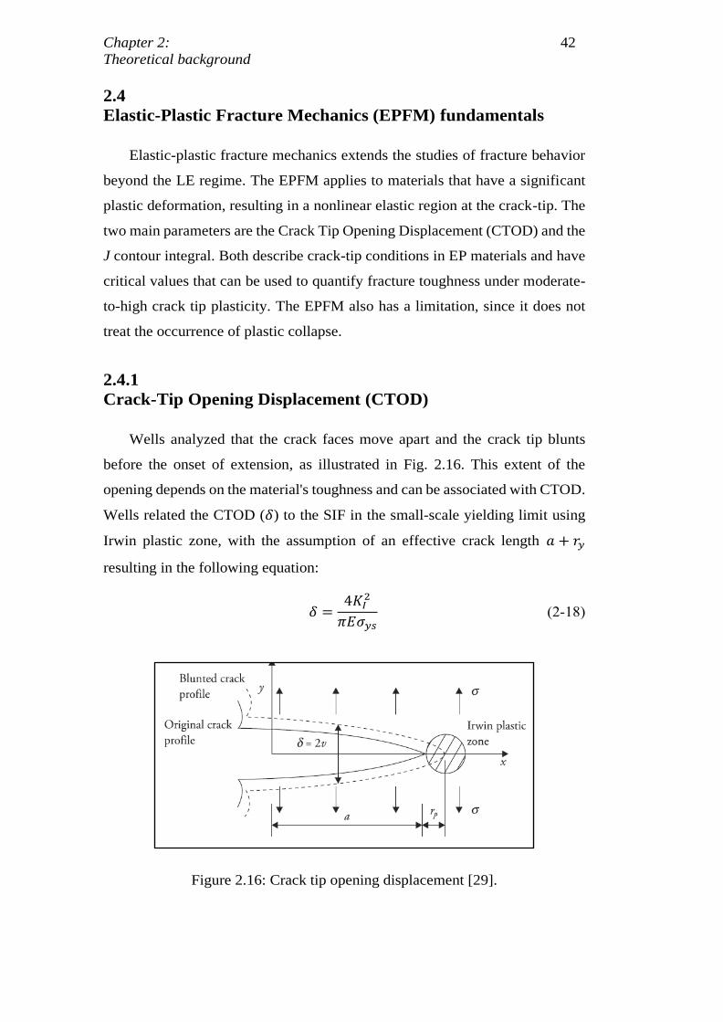
Wells analyzed that the crack faces move apart and the crack tip blunts

before the onset of extension, as illustrated in Fig. 2.16. This extent of the

opening depends on the material's toughness and can be associated with CTOD.

Wells related the CTOD (𝛿) to the SIF in the small-scale yielding limit using

Irwin plastic zone, with the assumption of an effective crack length 𝑎 + 𝑟𝑦

resulting in the following equation:

𝛿 =4𝐾𝐼

2

𝜋𝐸𝜎𝑦𝑠(2-18)

Figure 2.16: Crack tip opening displacement [29].

DBD


Chapter 2: 43


The CTOD parameter is not valid for LEFM, since it requires a plastic zone

at the crack tip, that allows the displacement of the two crack faces. Dugdale

and Dawes also did studies to measure CTOD. Dugdale used the strip-yield

theory by assuming a slender pz at the crack tip in nonhardening materials and

plane stress that have finite stress. Dawes estimated CTOD by measuring the

Crack Mouth Opening Displacement (CMOD) and using similar triangles

construction to relate the CMOD with CTOD. He developed a CTOD design

curve, which is a semiempirical fracture mechanics methodology for welded

steel structures [30].

2.4.2

J-Integral

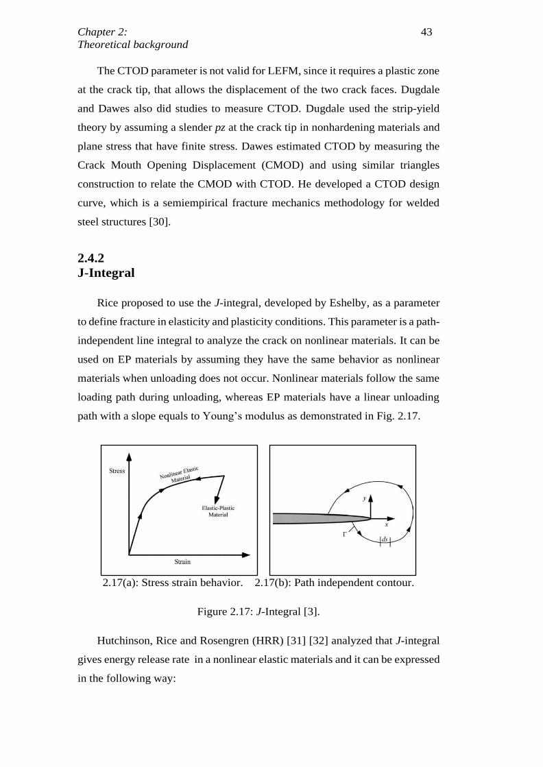
Rice proposed to use the J-integral, developed by Eshelby, as a parameter

to define fracture in elasticity and plasticity conditions. This parameter is a path-

independent line integral to analyze the crack on nonlinear materials. It can be

used on EP materials by assuming they have the same behavior as nonlinear

materials when unloading does not occur. Nonlinear materials follow the same

loading path during unloading, whereas EP materials have a linear unloading

path with a slope equals to Young’s modulus as demonstrated in Fig. 2.17.

2.17(a): Stress strain behavior. 2.17(b): Path independent contour.

Figure 2.17: J-Integral [3].

Hutchinson, Rice and Rosengren (HRR) [31] [32] analyzed that J-integral

gives energy release rate in a nonlinear elastic materials and it can be expressed

in the following way:

DBD


Chapter 2: 44


𝐽 = ∫ (𝑈𝑑𝑦 +𝑇𝑖𝜕𝑢𝑖

𝜕𝑥𝑑𝑠)

Γ

(2-19)

where 𝑈 is the strain energy density given by Eq. 2-20, 𝑇𝑖 are the traction vector

components at a point on the contour defined by Eq. 2-21, 𝑢𝑖 are displacement

vector components, ds is the length increment along the contour of the

counterclockwise path Γ. The stress and strain tensors are denoted as σ𝑖𝑗 and

ϵ𝑖𝑗 respectively, and 𝑛𝑗 are the components of the unit vector normal to Γ.

𝑈 = ∫ 𝜎𝑖𝑗𝑑𝜖𝑖𝑗

𝜖𝑖𝑗

0

(2-20)

𝑇𝑖 = 𝜎𝑖𝑗𝑛𝑗 (2-21)

Both J and G represents the potential energy that is released from the

structure when the crack grows, although G is only for LE conditions while J

can be used on LE and EP materials. Also, it is possible to correlate J with

CTOD using the following equation:

𝐽 = 𝑚𝜎𝑦𝑠𝛿 (2-22)

where m is a dimensionless constant that depends on the material properties and

stress state.

2.4.3

J-R Curve

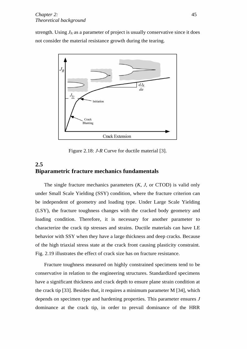
For EPFM, the fracture toughness JIc does not characterize a catastrophic

failure as KIc for LEFM. Instead, it indicates the initiation of stable crack growth

in EP materials and have a significant variation with the cracked body geometry

and loading condition. As the crack size increases, the material resistance also

increases, resulting in the J-resistance or J-R Curve that relates J with crack

extension (Fig. 2.18). The initial part of the curve has a linear relationship due

to crack blunting until the crack initiate. After that, the relation becomes

nonlinear up to material failure by tearing instability or plastic collapse.

The actual point of crack initiation is usually ill-defined [3]. Therefore, the

arbitrary definition is the intersection of the J-R curve with the 0.2% offset yield

DBD


Chapter 2: 45


strength. Using JIc as a parameter of project is usually conservative since it does

not consider the material resistance growth during the tearing.

Figure 2.18: J-R Curve for ductile material [3].

2.5

Biparametric fracture mechanics fundamentals

The single fracture mechanics parameters (K, J, or CTOD) is valid only

under Small Scale Yielding (SSY) condition, where the fracture criterion can

be independent of geometry and loading type. Under Large Scale Yielding

(LSY), the fracture toughness changes with the cracked body geometry and

loading condition. Therefore, it is necessary for another parameter to

characterize the crack tip stresses and strains. Ductile materials can have LE

behavior with SSY when they have a large thickness and deep cracks. Because

of the high triaxial stress state at the crack front causing plasticity constraint.

Fig. 2.19 illustrates the effect of crack size has on fracture resistance.

Fracture toughness measured on highly constrained specimens tend to be

conservative in relation to the engineering structures. Standardized specimens

have a significant thickness and crack depth to ensure plane strain condition at

the crack tip [33]. Besides that, it requires a minimum parameter M [34], which

depends on specimen type and hardening properties. This parameter ensures J

dominance at the crack tip, in order to prevail dominance of the HRR

DBD


Chapter 2: 46


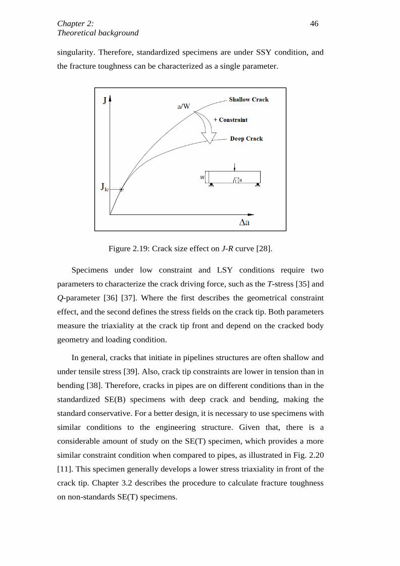
singularity. Therefore, standardized specimens are under SSY condition, and

the fracture toughness can be characterized as a single parameter.

Figure 2.19: Crack size effect on J-R curve [28].

Specimens under low constraint and LSY conditions require two

parameters to characterize the crack driving force, such as the T-stress [35] and

Q-parameter [36] [37]. Where the first describes the geometrical constraint

effect, and the second defines the stress fields on the crack tip. Both parameters

measure the triaxiality at the crack tip front and depend on the cracked body

geometry and loading condition.

In general, cracks that initiate in pipelines structures are often shallow and

under tensile stress [39]. Also, crack tip constraints are lower in tension than in

bending [38]. Therefore, cracks in pipes are on different conditions than in the

standardized SE(B) specimens with deep crack and bending, making the

standard conservative. For a better design, it is necessary to use specimens with

similar conditions to the engineering structure. Given that, there is a

considerable amount of study on the SE(T) specimen, which provides a more

similar constraint condition when compared to pipes, as illustrated in Fig. 2.20

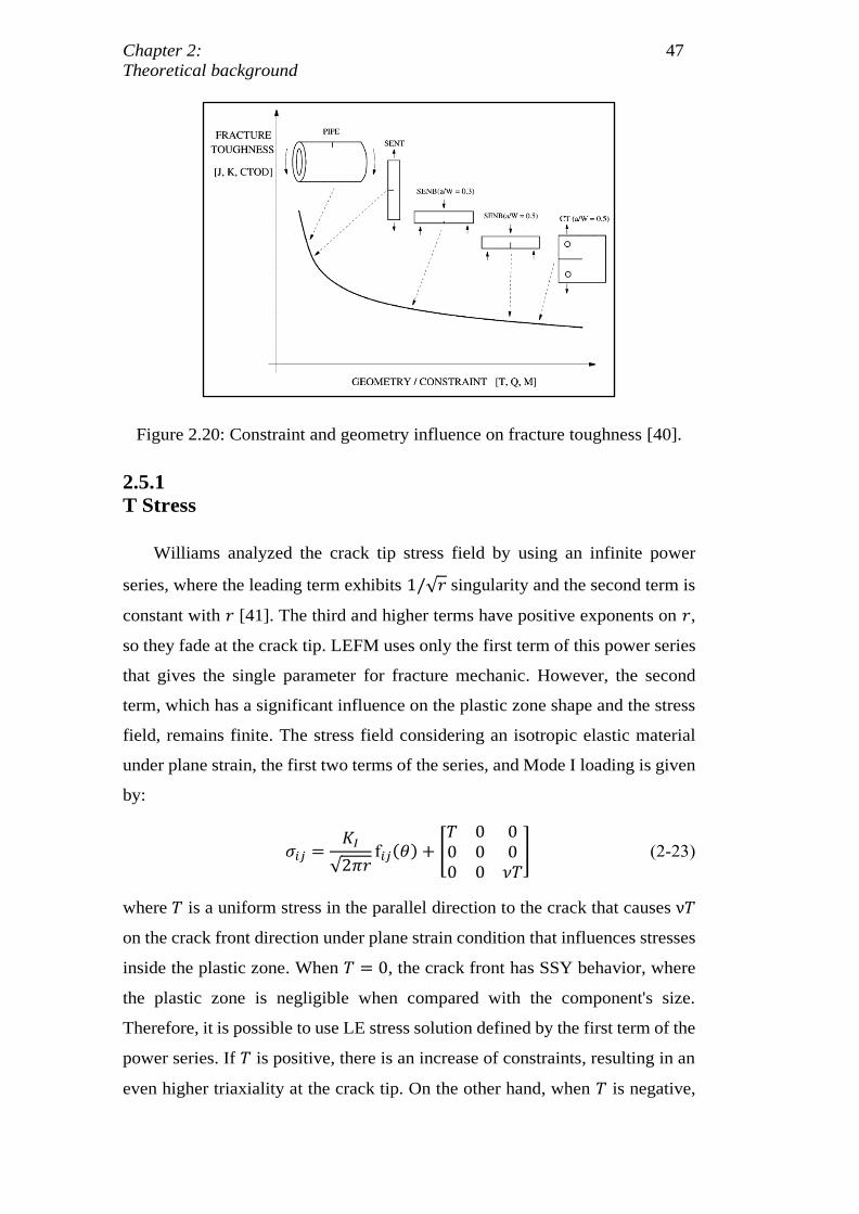
[11]. This specimen generally develops a lower stress triaxiality in front of the

crack tip. Chapter 3.2 describes the procedure to calculate fracture toughness

on non-standards SE(T) specimens.

DBD


Chapter 2: 47


Figure 2.20: Constraint and geometry influence on fracture toughness [40].

2.5.1

T Stress

Williams analyzed the crack tip stress field by using an infinite power

series, where the leading term exhibits 1/√𝑟 singularity and the second term is

constant with 𝑟 [41]. The third and higher terms have positive exponents on 𝑟,

so they fade at the crack tip. LEFM uses only the first term of this power series

that gives the single parameter for fracture mechanic. However, the second

term, which has a significant influence on the plastic zone shape and the stress

field, remains finite. The stress field considering an isotropic elastic material

under plane strain, the first two terms of the series, and Mode I loading is given

by:

𝜎𝑖𝑗 =𝐾𝐼

√2𝜋𝑟f𝑖𝑗(𝜃) + [

𝑇 0 00 0 00 0 𝜈𝑇

] (2-23)

where 𝑇 is a uniform stress in the parallel direction to the crack that causes ν𝑇

on the crack front direction under plane strain condition that influences stresses

inside the plastic zone. When 𝑇 = 0, the crack front has SSY behavior, where

the plastic zone is negligible when compared with the component's size.

Therefore, it is possible to use LE stress solution defined by the first term of the

power series. If 𝑇 is positive, there is an increase of constraints, resulting in an

even higher triaxiality at the crack tip. On the other hand, when 𝑇 is negative,

DBD


Chapter 2: 48


these constraints significantly decrease, thus it is necessary to use the bi-

parameter methodology.

The 𝑇-stress is an elastic parameter, so this methodology fails under EP

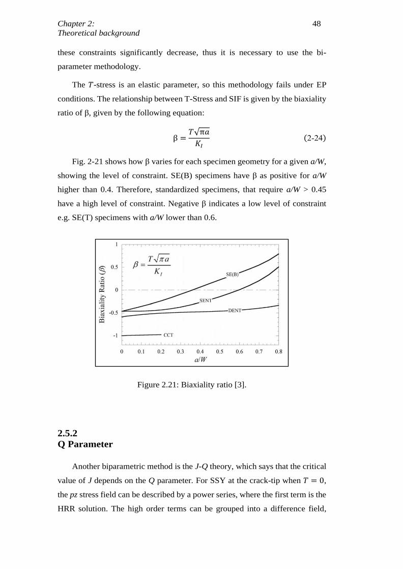
conditions. The relationship between T-Stress and SIF is given by the biaxiality

ratio of β, given by the following equation:

β =𝑇√π𝑎

𝐾𝐼

(2-24)

Fig. 2-21 shows how β varies for each specimen geometry for a given a/W,

showing the level of constraint. SE(B) specimens have β as positive for a/W

higher than 0.4. Therefore, standardized specimens, that require a/W > 0.45

have a high level of constraint. Negative β indicates a low level of constraint

e.g. SE(T) specimens with a/W lower than 0.6.

Figure 2.21: Biaxiality ratio [3].

2.5.2

Q Parameter

Another biparametric method is the J-Q theory, which says that the critical

value of J depends on the Q parameter. For SSY at the crack-tip when 𝑇 = 0,

the pz stress field can be described by a power series, where the first term is the

HRR solution. The high order terms can be grouped into a difference field,

DBD


Chapter 2: 49


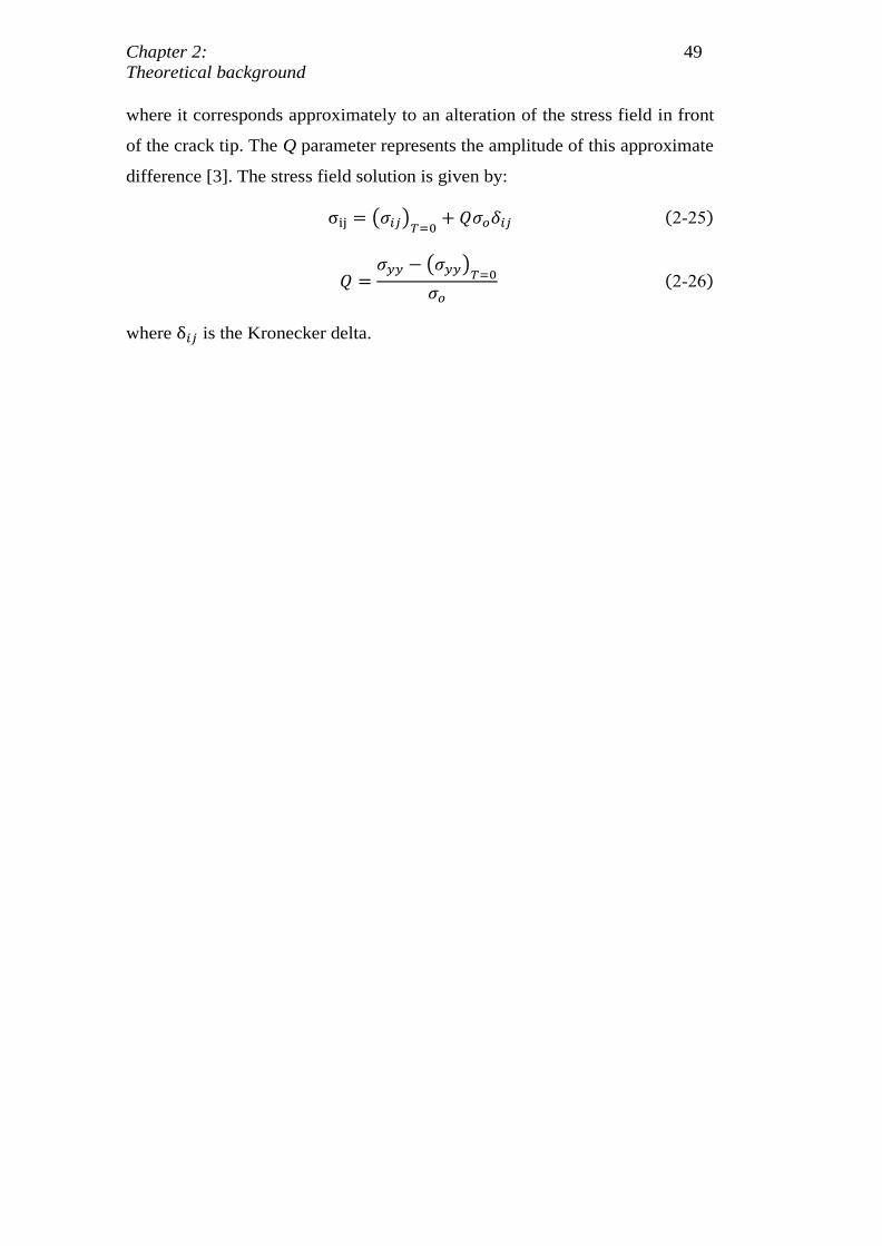
where it corresponds approximately to an alteration of the stress field in front

of the crack tip. The Q parameter represents the amplitude of this approximate

difference [3]. The stress field solution is given by:

σij = (𝜎𝑖𝑗)𝑇=0

+ 𝑄𝜎𝑜𝛿𝑖𝑗 (2-25)

𝑄 =𝜎𝑦𝑦 − (𝜎𝑦𝑦)

𝑇=0

𝜎𝑜

(2-26)

where δ𝑖𝑗 is the Kronecker delta.

DBD


Chapter 3:

Standard procedures to measure fracture toughness

3.


With the goal to measure fracture toughness under LE or EP conditions,

ASTM developed its E1820 standard [7], which lists procedures and guidelines

to obtain properties like e.g. JIc. Its test procedures specify how to load fatigue

pre-cracked specimens until forcing unstable or stable crack extension (Section

3.1.1). This work focus is on stable crack extension by crack tearing. Fracture

toughness results from the J-R curve that relates applied J-integral values with

crack increments. The standard provides two methods for measuring crack

increments, the basic and the resistance curve procedures. The basic procedure

requires multiple specimens to develop a plot from which a single toughness

value associated with crack tearing initiation can be evaluated. The resistance

curve procedure requires only a single specimen in which successive crack

increments are measured using the elastic unloading compliance method (see

Section 3.1.2). In this thesis, the chosen procedure is the compliance technique,

because level 3 of the API 579 fitness-for-purpose guide requires a well-defined

crack tearing resistance curve to characterize the material toughness. Finally, it

should be mentioned that there are many other standards for measuring fracture

toughness, for instance, ASTM E399 [5], ASTM E1290 [6], BS 7448 [8], and

EFAM GTP [9].

3.1

Fracture toughness specimens

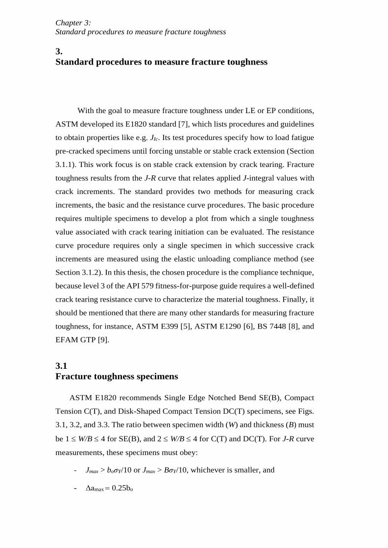
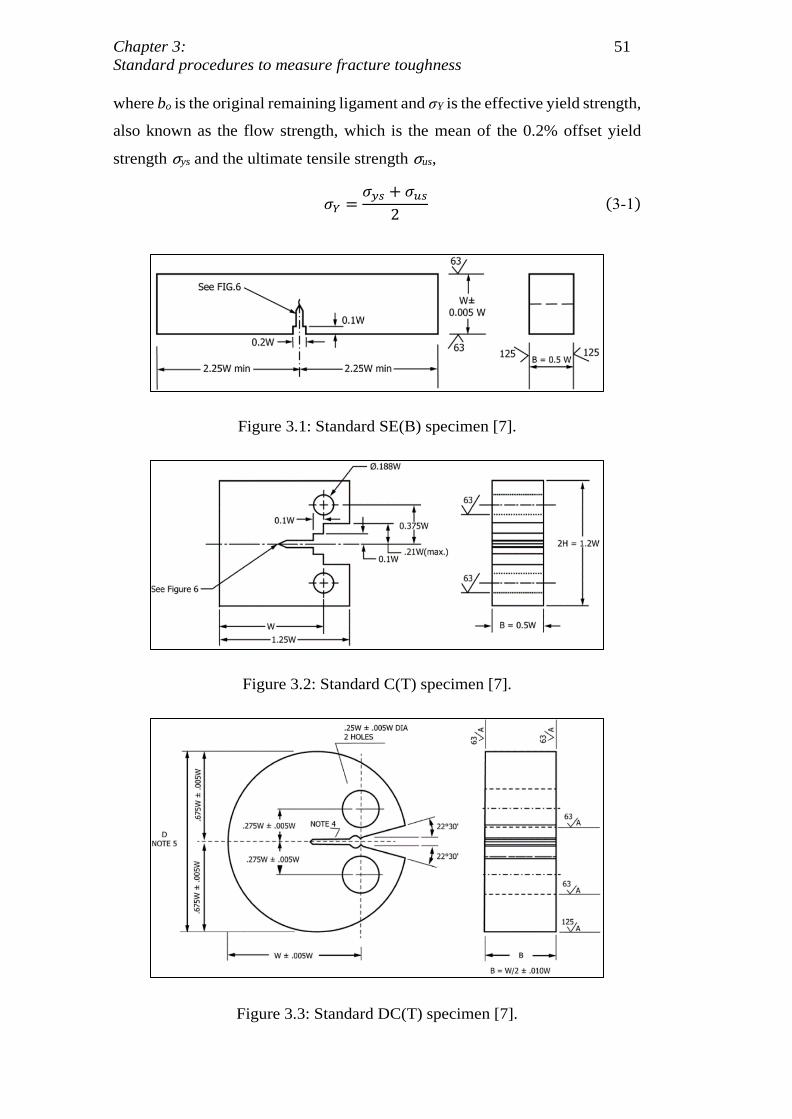
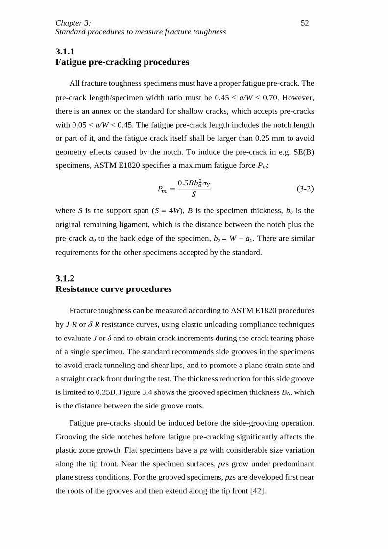
ASTM E1820 recommends Single Edge Notched Bend SE(B), Compact

Tension C(T), and Disk-Shaped Compact Tension DC(T) specimens, see Figs.

3.1, 3.2, and 3.3. The ratio between specimen width (W) and thickness (B) must

be 1 W/B 4 for SE(B), and 2 W/B 4 for C(T) and DC(T). For J-R curve

measurements, these specimens must obey:

- Jmax > boσY/10 or Jmax > BσY/10, whichever is smaller, and

- Δamax = 0.25bo

DBD


Chapter 3: 51


where bo is the original remaining ligament and σY is the effective yield strength,

also known as the flow strength, which is the mean of the 0.2% offset yield

strength σys and the ultimate tensile strength σus,

𝜎𝑌 =𝜎𝑦𝑠 + 𝜎𝑢𝑠

2(3-1)

Figure 3.1: Standard SE(B) specimen [7].

Figure 3.2: Standard C(T) specimen [7].

Figure 3.3: Standard DC(T) specimen [7].

DBD


Chapter 3: 52


3.1.1

Fatigue pre-cracking procedures

All fracture toughness specimens must have a proper fatigue pre-crack. The

pre-crack length/specimen width ratio must be 0.45 a/W 0.70. However,

there is an annex on the standard for shallow cracks, which accepts pre-cracks

with 0.05 < a/W < 0.45. The fatigue pre-crack length includes the notch length

or part of it, and the fatigue crack itself shall be larger than 0.25 mm to avoid

geometry effects caused by the notch. To induce the pre-crack in e.g. SE(B)

specimens, ASTM E1820 specifies a maximum fatigue force Pm:

𝑃𝑚 =0.5𝐵𝑏𝑜

2𝜎𝑌

𝑆(3-2)

where S is the support span (S = 4W), B is the specimen thickness, bo is the

original remaining ligament, which is the distance between the notch plus the

pre-crack ao to the back edge of the specimen, bo = W − ao. There are similar

requirements for the other specimens accepted by the standard.

3.1.2

Resistance curve procedures

Fracture toughness can be measured according to ASTM E1820 procedures

by J-R or -R resistance curves, using elastic unloading compliance techniques

to evaluate J or δ and to obtain crack increments during the crack tearing phase

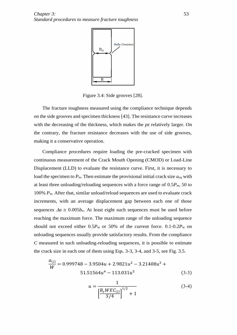
of a single specimen. The standard recommends side grooves in the specimens

to avoid crack tunneling and shear lips, and to promote a plane strain state and

a straight crack front during the test. The thickness reduction for this side groove

is limited to 0.25B. Figure 3.4 shows the grooved specimen thickness BN, which

is the distance between the side groove roots.

Fatigue pre-cracks should be induced before the side-grooving operation.

Grooving the side notches before fatigue pre-cracking significantly affects the

plastic zone growth. Flat specimens have a pz with considerable size variation

along the tip front. Near the specimen surfaces, pzs grow under predominant

plane stress conditions. For the grooved specimens, pzs are developed first near

the roots of the grooves and then extend along the tip front [42].

DBD


Chapter 3: 53


Figure 3.4: Side grooves [28].

The fracture toughness measured using the compliance technique depends

on the side grooves and specimen thickness [43]. The resistance curve increases

with the decreasing of the thickness, which makes the pz relatively larger. On

the contrary, the fracture resistance decreases with the use of side grooves,

making it a conservative operation.

Compliance procedures require loading the pre-cracked specimen with

continuous measurement of the Crack Mouth Opening (CMOD) or Load-Line

Displacement (LLD) to evaluate the resistance curve. First, it is necessary to

load the specimen to Pm. Then estimate the provisional initial crack size aoq with

at least three unloading/reloading sequences with a force range of 0.5Pm, 50 to

100% Pm. After that, similar unload/reload sequences are used to evaluate crack

increments, with an average displacement gap between each one of those

sequences a 0.005bo. At least eight such sequences must be used before

reaching the maximum force. The maximum range of the unloading sequence

should not exceed either 0.5Pm or 50% of the current force. 0.1-0.2Pm on

unloading sequences usually provide satisfactory results. From the compliance

C measured in such unloading-reloading sequences, it is possible to estimate

the crack size in each one of them using Eqs. 3-3, 3-4, and 3-5, see Fig. 3.5.

𝑎(𝑖)

𝑊= 0.999748 − 3.9504𝑢 + 2.9821𝑢2 − 3.21408𝑢3 +

51.51564𝑢4 − 113.031𝑢5 (3-3)

𝑢 =1

[𝐵𝑒𝑊𝐸𝐶(𝑖)

𝑆/4]

1/2

+ 1

(3-4)

DBD


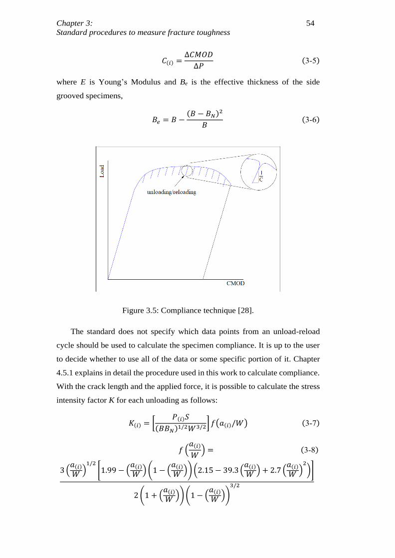
Chapter 3: 54


𝐶(𝑖) =Δ𝐶𝑀𝑂𝐷

Δ𝑃(3-5)

where E is Young’s Modulus and Be is the effective thickness of the side

grooved specimens,

𝐵𝑒 = 𝐵 −(𝐵 − 𝐵𝑁)2

𝐵(3-6)

Figure 3.5: Compliance technique [28].

The standard does not specify which data points from an unload-reload

cycle should be used to calculate the specimen compliance. It is up to the user

to decide whether to use all of the data or some specific portion of it. Chapter

4.5.1 explains in detail the procedure used in this work to calculate compliance.

With the crack length and the applied force, it is possible to calculate the stress

intensity factor K for each unloading as follows:

𝐾(𝑖) = [𝑃(𝑖)𝑆

(𝐵𝐵𝑁)1/2𝑊3/2] 𝑓(𝑎(𝑖)/𝑊) (3-7)

𝑓 (𝑎(𝑖)

𝑊) = (3-8)

3 (𝑎(𝑖)

𝑊 )1/2

[1.99 − (𝑎(𝑖)

𝑊 ) (1 − (𝑎(𝑖)

𝑊 )) (2.15 − 39.3 (𝑎(𝑖)

𝑊 ) + 2.7 (𝑎(𝑖)

𝑊 )2

)]

2 (1 + (𝑎(𝑖)

𝑊 )) (1 − (𝑎(𝑖)

𝑊 ))

3/2

DBD


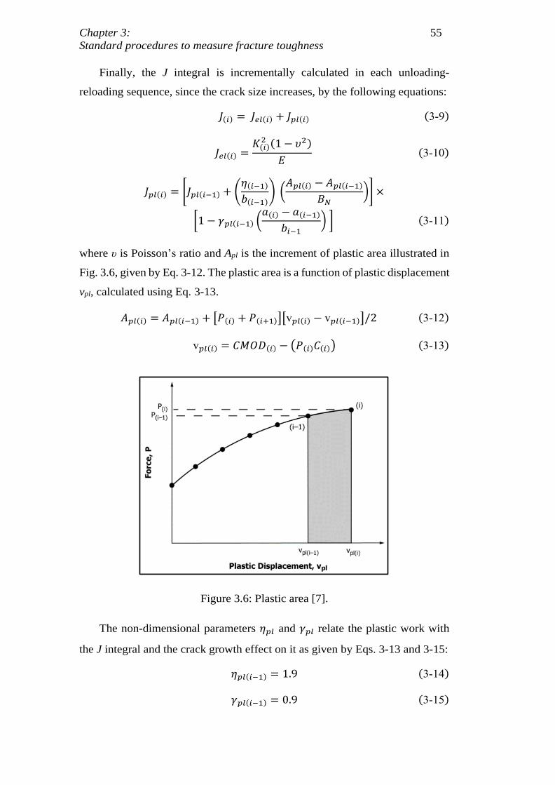
Chapter 3: 55


Finally, the J integral is incrementally calculated in each unloading-

reloading sequence, since the crack size increases, by the following equations:

𝐽(𝑖) = 𝐽𝑒𝑙(𝑖) + 𝐽𝑝𝑙(𝑖) (3-9)

𝐽𝑒𝑙(𝑖) =𝐾(𝑖)

2 (1 − 𝜐2)

𝐸(3-10)

𝐽𝑝𝑙(𝑖) = [𝐽𝑝𝑙(𝑖−1) + (𝜂(𝑖−1)

𝑏(𝑖−1)) (

𝐴𝑝𝑙(𝑖) − 𝐴𝑝𝑙(𝑖−1)

𝐵𝑁)] ×

[1 − 𝛾𝑝𝑙(𝑖−1) (𝑎(𝑖) − 𝑎(𝑖−1)

𝑏𝑖−1) ] (3-11)

where υ is Poisson’s ratio and Apl is the increment of plastic area illustrated in

Fig. 3.6, given by Eq. 3-12. The plastic area is a function of plastic displacement

vpl, calculated using Eq. 3-13.

𝐴𝑝𝑙(𝑖) = 𝐴𝑝𝑙(𝑖−1) + [𝑃(𝑖) + 𝑃(𝑖+1)][v𝑝𝑙(𝑖) − v𝑝𝑙(𝑖−1)]/2 (3-12)

v𝑝𝑙(𝑖) = 𝐶𝑀𝑂𝐷(𝑖) − (𝑃(𝑖)𝐶(𝑖)) (3-13)

Figure 3.6: Plastic area [7].

The non-dimensional parameters 𝜂𝑝𝑙 and 𝛾𝑝𝑙 relate the plastic work with

the J integral and the crack growth effect on it as given by Eqs. 3-13 and 3-15:

𝜂𝑝𝑙(𝑖−1) = 1.9 (3-14)

𝛾𝑝𝑙(𝑖−1) = 0.9 (3-15)

DBD


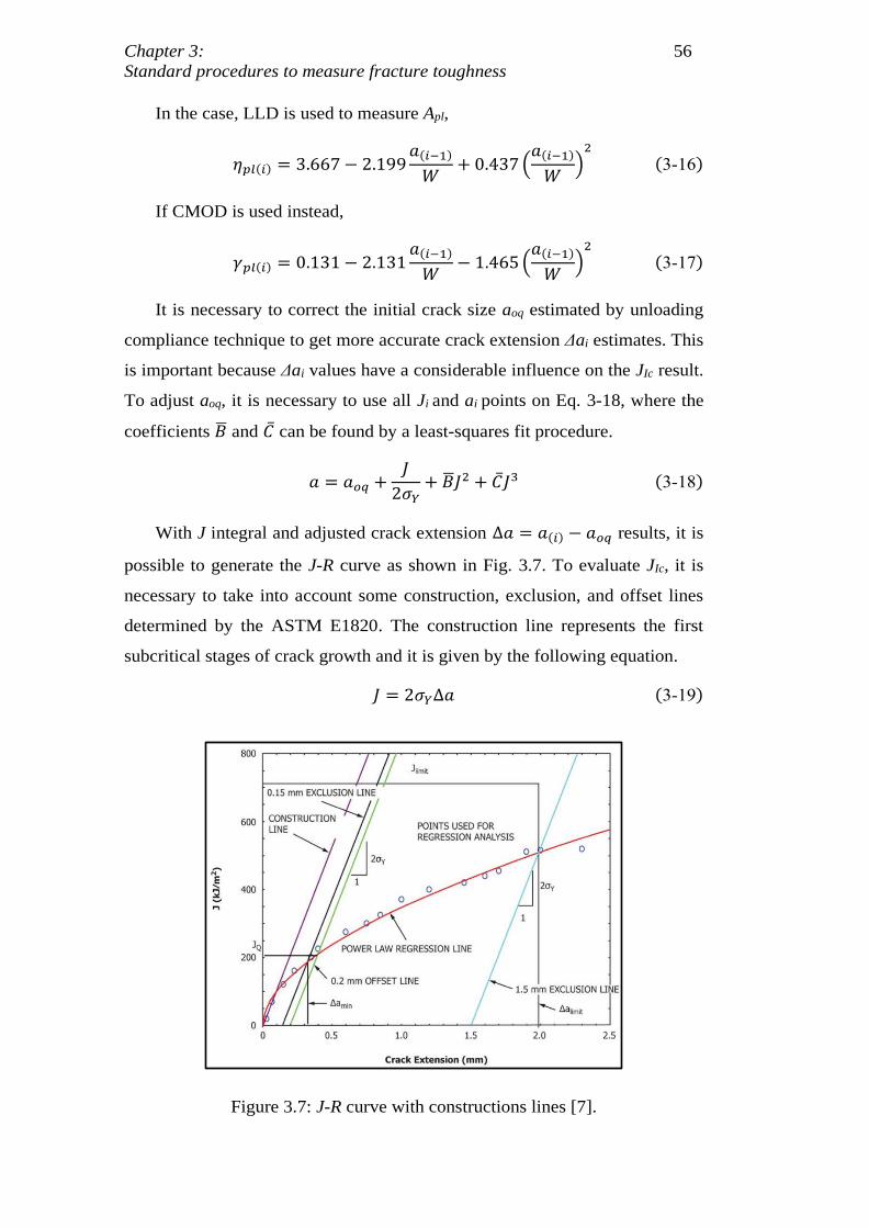
Chapter 3: 56


In the case, LLD is used to measure Apl,

𝜂𝑝𝑙(𝑖) = 3.667 − 2.199𝑎(𝑖−1)

𝑊+ 0.437 (

𝑎(𝑖−1)

𝑊)

2

(3-16)

If CMOD is used instead,

𝛾𝑝𝑙(𝑖) = 0.131 − 2.131𝑎(𝑖−1)

𝑊− 1.465 (

𝑎(𝑖−1)

𝑊)

2

(3-17)

It is necessary to correct the initial crack size aoq estimated by unloading

compliance technique to get more accurate crack extension Δai estimates. This

is important because Δai values have a considerable influence on the JIc result.

To adjust aoq, it is necessary to use all Ji and ai points on Eq. 3-18, where the

coefficients �̅� and �̅� can be found by a least-squares fit procedure.

𝑎 = 𝑎𝑜𝑞 +𝐽

2𝜎𝑌+ �̅�𝐽2 + �̅�𝐽3 (3-18)

With J integral and adjusted crack extension Δ𝑎 = 𝑎(𝑖) − 𝑎𝑜𝑞 results, it is

possible to generate the J-R curve as shown in Fig. 3.7. To evaluate JIc, it is

necessary to take into account some construction, exclusion, and offset lines

determined by the ASTM E1820. The construction line represents the first

subcritical stages of crack growth and it is given by the following equation.

𝐽 = 2𝜎𝑌Δ𝑎 (3-19)

Figure 3.7: J-R curve with constructions lines [7].

DBD


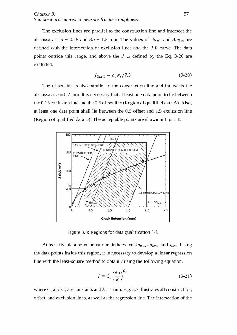
Chapter 3: 57


The exclusion lines are parallel to the construction line and intersect the

abscissa at Δa = 0.15 and Δa = 1.5 mm. The values of Δamin and Δalimit are

defined with the intersection of exclusion lines and the J-R curve. The data

points outside this range, and above the Jlimit defined by the Eq. 3-20 are

excluded.

𝐽𝑙𝑖𝑚𝑖𝑡 = 𝑏𝑜𝜎𝑌/7.5 (3-20)

The offset line is also parallel to the construction line and intersects the

abscissa at a = 0.2 mm. It is necessary that at least one data point to lie between

the 0.15 exclusion line and the 0.5 offset line (Region of qualified data A). Also,

at least one data point shall lie between the 0.5 offset and 1.5 exclusion line

(Region of qualified data B). The acceptable points are shown in Fig. 3.8.

Figure 3.8: Regions for data qualification [7].

At least five data points must remain between Δamin, Δalimit, and Jlimit. Using

the data points inside this region, it is necessary to develop a linear regression

line with the least-square method to obtain J using the following equation.

𝐽 = 𝐶1 (Δ𝑎

𝑘)

𝐶2

(3-21)

where C1 and C2 are constants and 𝑘 = 1 mm. Fig. 3.7 illustrates all construction,

offset, and exclusion lines, as well as the regression line. The intersection of the

DBD


Chapter 3: 58


0.2 offset and the regression lines defines JIc and ΔaIc. For the qualification of

the data, the following requirement must be satisfied:

- B > 10JIc/σY

- bo > 10JIc/σY

Finally, it is possible to evaluate KJIc by the following equation.

𝐾𝐽𝐼𝑐 = √𝐸𝐽𝐼𝑐

1 − 𝜐2(3-22)

3.1.3

Optical crack size measurements

After finishing the J-R test, it is necessary to break the specimen with care

to minimize additional deformations, e.g. cooling it in liquid nitrogen to ensure

brittle fractures. The crack front must be divided into nine equally spaced points

centered about the specimen centerline, extending it to 0.005W from the side

groove root, or the surface of plane-sided specimens. Next, the size of the

fatigue pre-crack ao and the stable crack extension ap must be measured in each

section. The difference between the measured ao and the estimated aoq shall not

be more than 0.01W or 0.5 mm. Using the mean in each section, it is possible

to estimate the physical crack increment Δap = ap - ao. None of these

measurements shall differ by more than 0.05B.

3.2

Procedure for SE(T) specimens

Standardized specimens have high transversal constraints, and thus yield

conservative values of fracture toughness for use in less constrained geometries

like cracked pipes or pressure vessels much used in the petroleum industry. It

is necessary to use specimens with similar conditions to simulate their fracture

process in the laboratory. A good candidate for that is the SE(T) specimen since

it has a strong similarity in crack-tip stress and strain fields to the mentioned

structures. This specimen is already being widely used in the marine industry

to measure toughness.

DBD


Chapter 3: 59


In this work, less constrained fracture toughness measurements on clamped

SE(T) specimens follow the procedures developed by Cravero and Ruggieri

[21]. This method also evaluates J-R curves using the compliance technique.

Using results from finite element analyses and the least square method, these

authors proposed a fifth-order polynomial equation (Eq. 3-23) to estimate crack

length inside the range 0.1 ≤ a/W ≤ 0.7 on pin-loaded and clamped SE(T)

specimens. For pin-loaded specimens, the compliance 𝑢 is independent of H/W

ratio, where H is the distance between loading points. For clamped specimens,

it depends on H/W ratios for cracks deeper than 0.4a/W. The normalized

compliance is given by Eq. 3-24 [44].

𝑎/𝑊 = 𝛽0 + 𝛽1𝑢 + 𝛽2𝑢2 + 𝛽3𝑢3 + 𝛽4𝑢4 + 𝛽5𝑢5 (3-23)

𝑢 =1

1 + √𝐸′𝐵𝐶(3-24)

where β𝑖 are coefficients given for each type of SE(T) specimen and H/W ratio.

If side grooves are used, it is necessary to change the value of B to Be as in Eq.

3-24.

Shen et al. [45] also developed a solution to estimate crack lengths that

covers crack sizes over the range 0.05 ≤ a/W ≤ 0.95. However, its ninth order

polynomial equation makes it difficult to use on finite elements analyzes.

Moreover, to calculate the elastic SIF KI by Eq. 3-25, it is necessary to know

the non-dimensional geometry factor f(a/W) of the specimen. Several studies

show how to estimate this geometry factor on SE(T) specimens, but these

results have a limited range of a/W and H/W ratios. Cravero and Ruggieri

developed the fifth-order polynomial Eq. 3-26 to cover many geometries and

loading eccentricities on pin-loaded and clamped SE(T).

𝐾𝐼 =𝑃

𝐵√(𝑊)𝑓(𝑎/𝑊) (3-25)

𝑓(𝑎/𝑊) = 𝜉0 + 𝜉1(𝑎/𝑊) + 𝜉2(𝑎/𝑊)2 + 𝜉3(𝑎/𝑊)3 +

𝜉4(𝑎/𝑊)4 + 𝜉5(𝑎/𝑊)5 (3-26)

where ξ𝑖 are coefficients given for each type of SE(T) specimen, H/W ratio, and

loading point offset (LPO).

DBD


Chapter 3: 60


Finally, the parameters η𝑝𝑙 and γ𝑝𝑙, which depend on the computation of Apl

in Eq. 3-11, are also reevaluated for SE(T) specimens. Cravero and Ruggieri

analyzed these parameters using numerical experiences to evaluate the effect of

loading conditions and hardening properties. They concluded that 𝜂𝑝𝑙 obtained

from load versus CMOD curves is independent of hardening properties, and it

is less sensitive to the loading level when compared with 𝜂𝑝𝑙 obtained from load

versus LLD curves. The following equations provide polynomial fits for 𝜂𝑝𝑙

on clamped SE(T) specimen obtained from load versus CMOD curves (Eq. 3-

27) and from load versus LLD curves (Eq. 3-28). The polynomial fit of 𝛾𝑝𝑙 (Eq.

3-29) works for both curves.

𝜂𝐶𝐶𝑀𝑂𝐷 = 1.0398 − 0.6870(𝑎/𝑊) (3-27)

𝜂𝐶𝐿𝐿𝐷 = 𝐴 + 𝐵(𝑎/𝑊) + 𝐶(𝑎/𝑊)2 + 𝐷(𝑎/𝑊)3 (3-28)

𝛾𝐶 = (𝐴 − 1) + 𝐵(𝑎/𝑊) + 𝐶(𝑎/𝑊)2 + 𝐷(𝑎/𝑊)3 +

−𝐵 + (𝐵 − 2𝐶)(𝑎/𝑊) + (2𝐶 − 3𝐷)(𝑎/𝑊)2 + 3𝐷(𝑎/𝑊)3

𝐴 + 𝐵(𝑎/𝑊) + 𝐶(𝑎/𝑊)2 + 𝐷(𝑎/𝑊)3(3-29)

DBD


Chapter 4:

Experimental procedures and material characterization

4.


This chapter describes the tests performed on the API 5L X80 steel to

measure its mechanical properties needed in structural integrity analyses. All

specimens came from the same flat plate with 1100 mm length, 800 mm width,

and 21.85 mm thickness, as illustrated in Fig. 4.1. The specimens were cut in a

water jet machine to avoid heat-affected zones (HAZ) that could affect the

properties. Since the surface finish of the cuts is irregular, it was improved using

a milling machine. The experiments conducted in this work were:

- Metallography

- Chemical analysis

- Hardness test

- Tensile test

- JIc fracture toughness test

4.1

Metallography

A 202021.85 mm sample was cut from the steel plate steel for the

metallographic analysis. The sample surface was abraded with 150, 240, 320,

400, and 600 grit sandpaper, and then it was polished with diamond pastes of 6,

3, and 1μm in an Arotec metallographic polishing machine, see Fig. 4.2(a). The

sample (Fig. 4.2(b)) was cleaned in alcohol, air dried, etched with 2% nital, and

finally analyzed using an Axio ZEISS A1 optical microscope, see Fig. 4.2(c).

The X80 longitudinal and transversal microstructures are shown in Fig.

4.3(a) and (b). Due to the anisotropy caused by lamination, the microstructure

is slightly different in these two directions. The longitudinal grains are

elongated when compared to the transversal grains. The X80 microstructure is

composed by polygonal ferrite, quasi-polygonal ferrite, acicular ferrite,

DBD


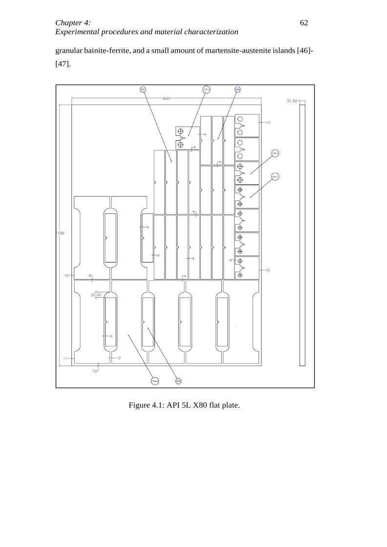
Chapter 4: 62


granular bainite-ferrite, and a small amount of martensite-austenite islands [46]-

[47].

Figure 4.1: API 5L X80 flat plate.

DBD


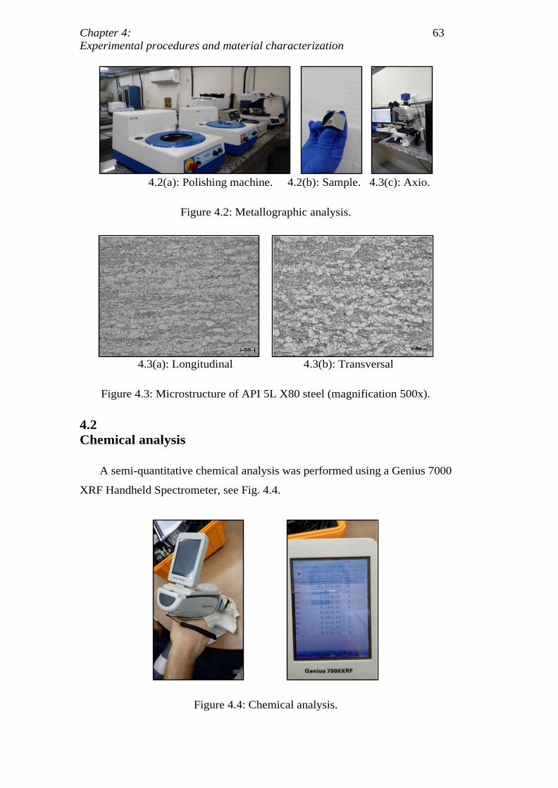
Chapter 4: 63


4.2(a): Polishing machine. 4.2(b): Sample. 4.3(c): Axio.

Figure 4.2: Metallographic analysis.

4.3(a): Longitudinal 4.3(b): Transversal

Figure 4.3: Microstructure of API 5L X80 steel (magnification 500x).

4.2

Chemical analysis

A semi-quantitative chemical analysis was performed using a Genius 7000

XRF Handheld Spectrometer, see Fig. 4.4.

Figure 4.4: Chemical analysis.

DBD


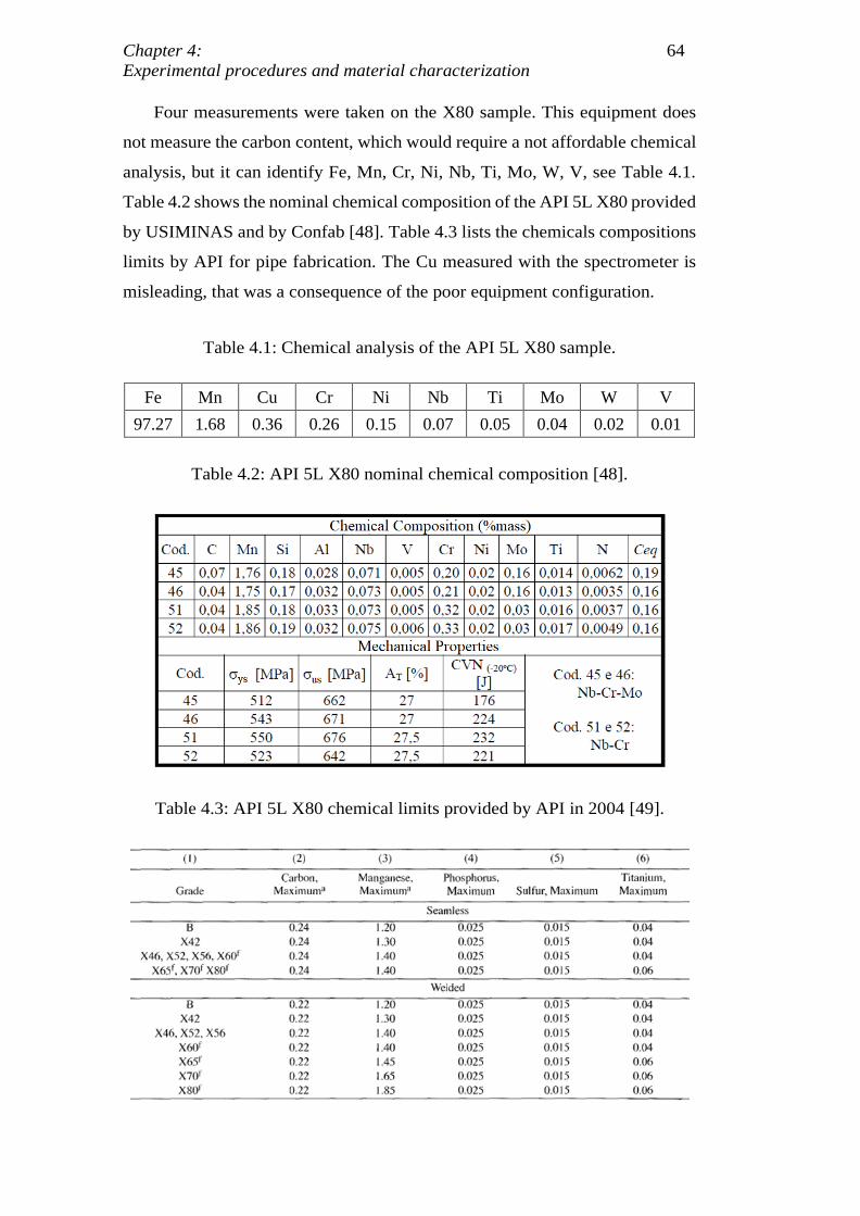
Chapter 4: 64


Four measurements were taken on the X80 sample. This equipment does

not measure the carbon content, which would require a not affordable chemical

analysis, but it can identify Fe, Mn, Cr, Ni, Nb, Ti, Mo, W, V, see Table 4.1.

Table 4.2 shows the nominal chemical composition of the API 5L X80 provided

by USIMINAS and by Confab [48]. Table 4.3 lists the chemicals compositions

limits by API for pipe fabrication. The Cu measured with the spectrometer is

misleading, that was a consequence of the poor equipment configuration.

Table 4.1: Chemical analysis of the API 5L X80 sample.

Fe Mn Cu Cr Ni Nb Ti Mo W V

97.27 1.68 0.36 0.26 0.15 0.07 0.05 0.04 0.02 0.01

Table 4.2: API 5L X80 nominal chemical composition [48].

Table 4.3: API 5L X80 chemical limits provided by API in 2004 [49].

DBD


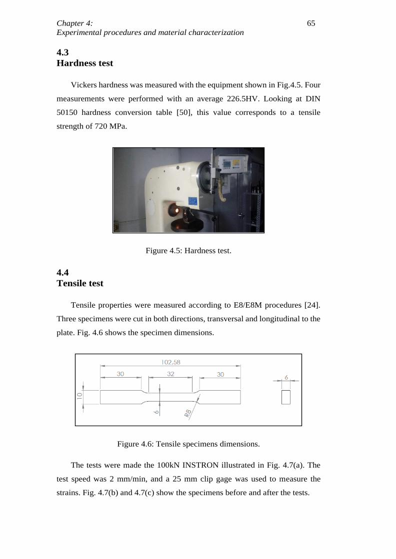
Chapter 4: 65


4.3

Hardness test

Vickers hardness was measured with the equipment shown in Fig.4.5. Four

measurements were performed with an average 226.5HV. Looking at DIN

50150 hardness conversion table [50], this value corresponds to a tensile

strength of 720 MPa.

Figure 4.5: Hardness test.

4.4

Tensile test

Tensile properties were measured according to E8/E8M procedures [24].

Three specimens were cut in both directions, transversal and longitudinal to the

plate. Fig. 4.6 shows the specimen dimensions.

Figure 4.6: Tensile specimens dimensions.

The tests were made the 100kN INSTRON illustrated in Fig. 4.7(a). The

test speed was 2 mm/min, and a 25 mm clip gage was used to measure the

strains. Fig. 4.7(b) and 4.7(c) show the specimens before and after the tests.

DBD


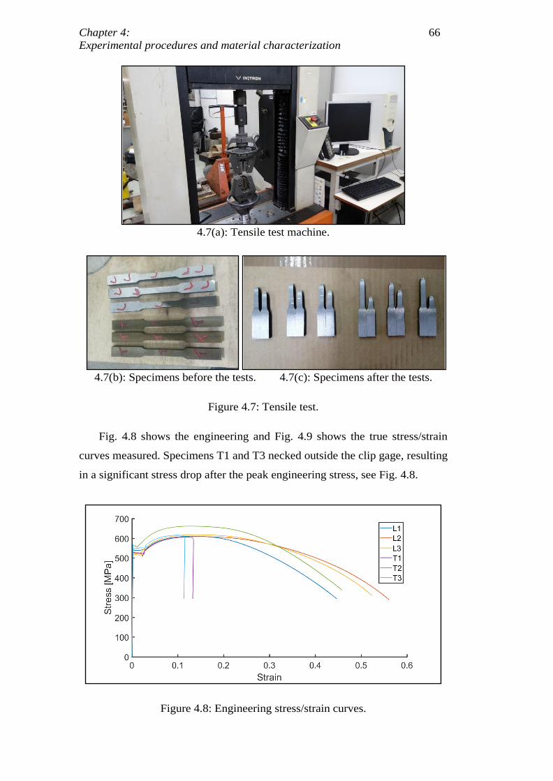
Chapter 4: 66


4.7(a): Tensile test machine.

4.7(b): Specimens before the tests. 4.7(c): Specimens after the tests.

Figure 4.7: Tensile test.

Fig. 4.8 shows the engineering and Fig. 4.9 shows the true stress/strain

curves measured. Specimens T1 and T3 necked outside the clip gage, resulting

in a significant stress drop after the peak engineering stress, see Fig. 4.8.

Figure 4.8: Engineering stress/strain curves.

DBD


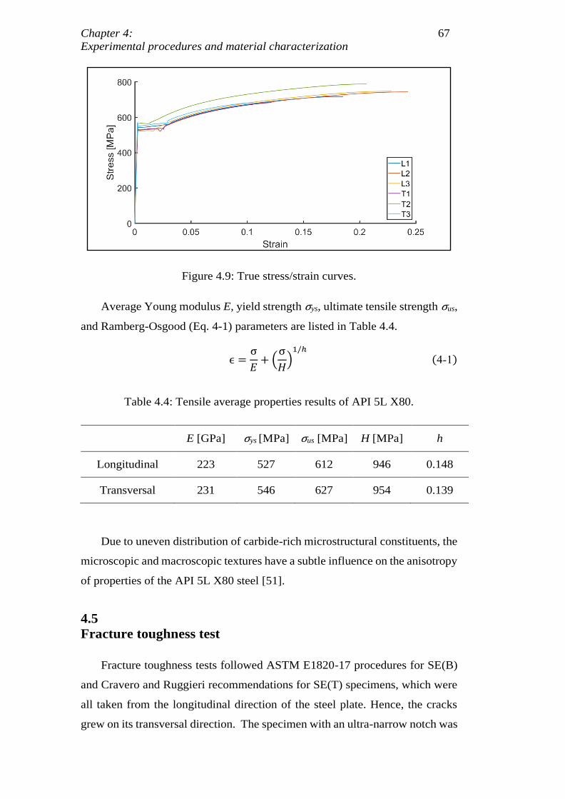
Chapter 4: 67


Figure 4.9: True stress/strain curves.

Average Young modulus E, yield strength σys, ultimate tensile strength σus,

and Ramberg-Osgood (Eq. 4-1) parameters are listed in Table 4.4.

ϵ =σ

𝐸+ (

σ

𝐻)

1/ℎ

(4-1)

Table 4.4: Tensile average properties results of API 5L X80.

E [GPa] σys [MPa] σus [MPa] H [MPa] h

Longitudinal 223 527 612 946 0.148

Transversal 231 546 627 954 0.139

Due to uneven distribution of carbide-rich microstructural constituents, the

microscopic and macroscopic textures have a subtle influence on the anisotropy

of properties of the API 5L X80 steel [51].

4.5

Fracture toughness test

Fracture toughness tests followed ASTM E1820-17 procedures for SE(B)

and Cravero and Ruggieri recommendations for SE(T) specimens, which were

all taken from the longitudinal direction of the steel plate. Hence, the cracks

grew on its transversal direction. The specimen with an ultra-narrow notch was

DBD


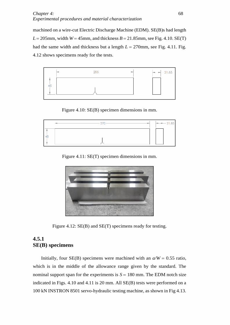
Chapter 4: 68


machined on a wire-cut Electric Discharge Machine (EDM). SE(B)s had length

L = 205mm, width W = 45mm, and thickness B = 21.85mm, see Fig. 4.10. SE(T)

had the same width and thickness but a length L = 270mm, see Fig. 4.11. Fig.

4.12 shows specimens ready for the tests.

Figure 4.10: SE(B) specimen dimensions in mm.

Figure 4.11: SE(T) specimen dimensions in mm.

Figure 4.12: SE(B) and SE(T) specimens ready for testing.

4.5.1

SE(B) specimens

Initially, four SE(B) specimens were machined with an a/W = 0.55 ratio,

which is in the middle of the allowance range given by the standard. The

nominal support span for the experiments is S = 180 mm. The EDM notch size

indicated in Figs. 4.10 and 4.11 is 20 mm. All SE(B) tests were performed on a

100 kN INSTRON 8501 servo-hydraulic testing machine, as shown in Fig 4.13.

DBD


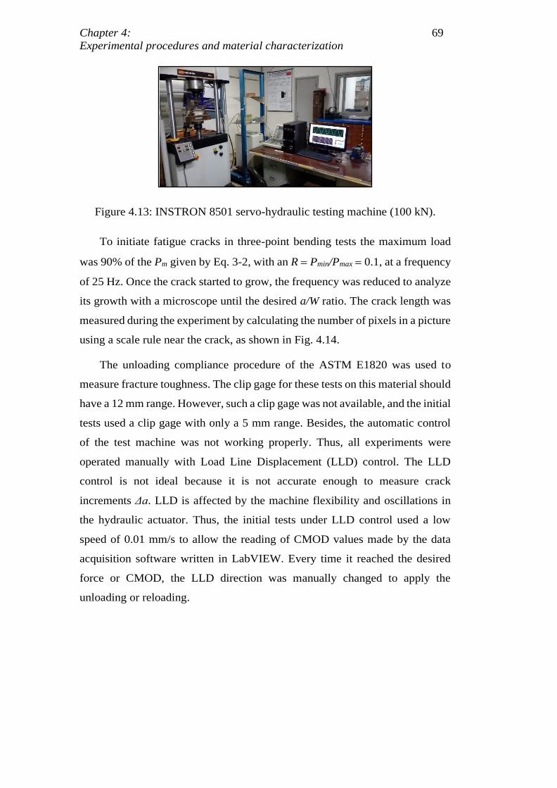
Chapter 4: 69


Figure 4.13: INSTRON 8501 servo-hydraulic testing machine (100 kN).

To initiate fatigue cracks in three-point bending tests the maximum load

was 90% of the Pm given by Eq. 3-2, with an R = Pmin/Pmax = 0.1, at a frequency

of 25 Hz. Once the crack started to grow, the frequency was reduced to analyze

its growth with a microscope until the desired a/W ratio. The crack length was

measured during the experiment by calculating the number of pixels in a picture

using a scale rule near the crack, as shown in Fig. 4.14.

The unloading compliance procedure of the ASTM E1820 was used to

measure fracture toughness. The clip gage for these tests on this material should

have a 12 mm range. However, such a clip gage was not available, and the initial

tests used a clip gage with only a 5 mm range. Besides, the automatic control

of the test machine was not working properly. Thus, all experiments were

operated manually with Load Line Displacement (LLD) control. The LLD

control is not ideal because it is not accurate enough to measure crack

increments Δa. LLD is affected by the machine flexibility and oscillations in

the hydraulic actuator. Thus, the initial tests under LLD control used a low

speed of 0.01 mm/s to allow the reading of CMOD values made by the data

acquisition software written in LabVIEW. Every time it reached the desired

force or CMOD, the LLD direction was manually changed to apply the

unloading or reloading.

DBD


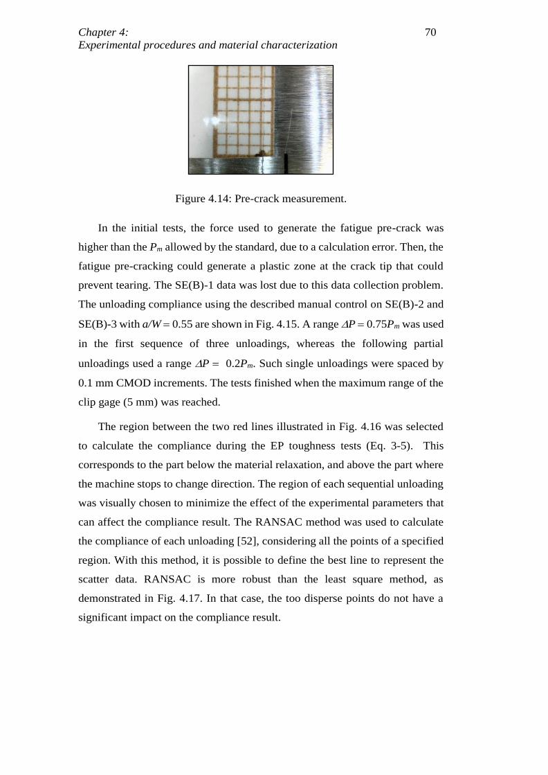
Chapter 4: 70


Figure 4.14: Pre-crack measurement.

In the initial tests, the force used to generate the fatigue pre-crack was

higher than the Pm allowed by the standard, due to a calculation error. Then, the

fatigue pre-cracking could generate a plastic zone at the crack tip that could

prevent tearing. The SE(B)-1 data was lost due to this data collection problem.

The unloading compliance using the described manual control on SE(B)-2 and

SE(B)-3 with a/W = 0.55 are shown in Fig. 4.15. A range P = 0.75Pm was used

in the first sequence of three unloadings, whereas the following partial

unloadings used a range P = 0.2Pm. Such single unloadings were spaced by

0.1 mm CMOD increments. The tests finished when the maximum range of the

clip gage (5 mm) was reached.

The region between the two red lines illustrated in Fig. 4.16 was selected

to calculate the compliance during the EP toughness tests (Eq. 3-5). This

corresponds to the part below the material relaxation, and above the part where

the machine stops to change direction. The region of each sequential unloading

was visually chosen to minimize the effect of the experimental parameters that

can affect the compliance result. The RANSAC method was used to calculate

the compliance of each unloading [52], considering all the points of a specified

region. With this method, it is possible to define the best line to represent the

scatter data. RANSAC is more robust than the least square method, as

demonstrated in Fig. 4.17. In that case, the too disperse points do not have a

significant impact on the compliance result.

DBD


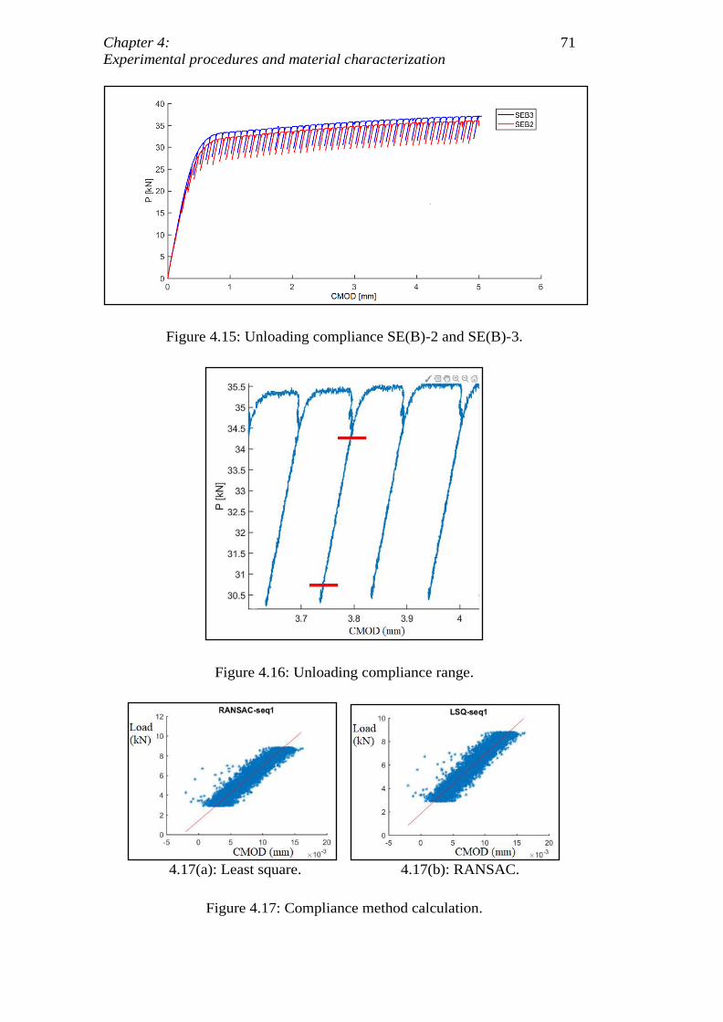
Chapter 4: 71


Figure 4.15: Unloading compliance SE(B)-2 and SE(B)-3.

Figure 4.16: Unloading compliance range.

4.17(a): Least square. 4.17(b): RANSAC.

Figure 4.17: Compliance method calculation.

DBD


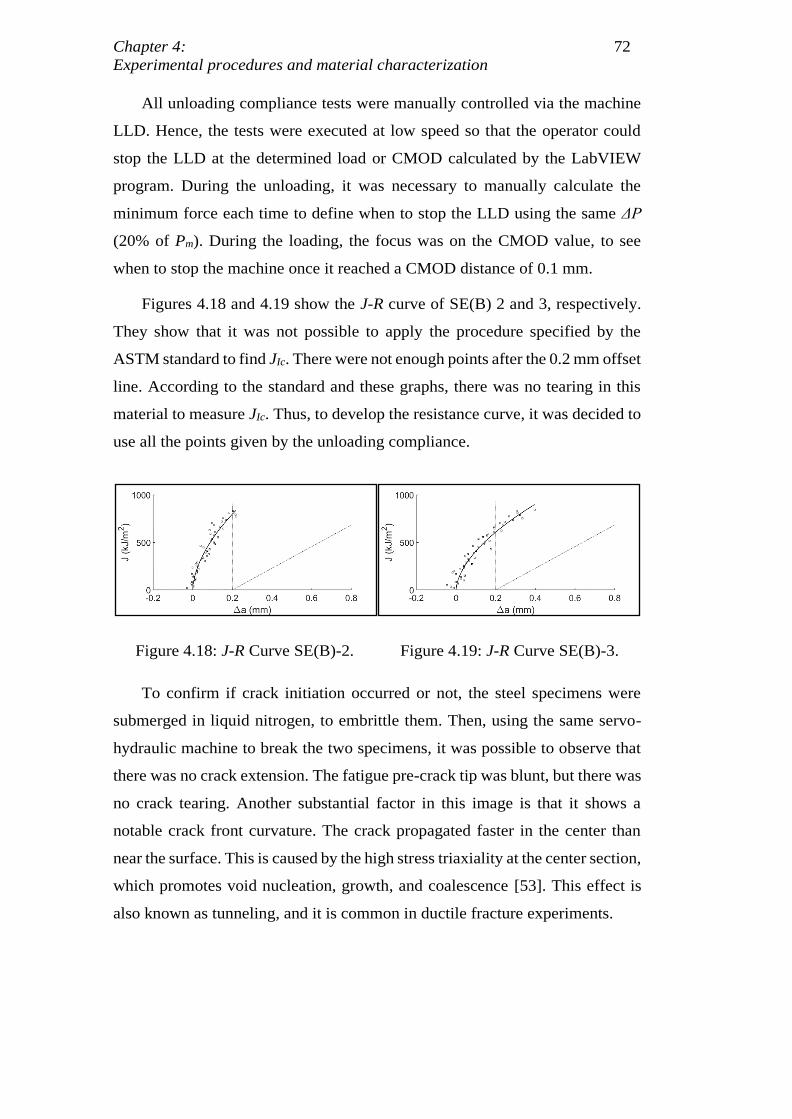
Chapter 4: 72


All unloading compliance tests were manually controlled via the machine

LLD. Hence, the tests were executed at low speed so that the operator could

stop the LLD at the determined load or CMOD calculated by the LabVIEW

program. During the unloading, it was necessary to manually calculate the

minimum force each time to define when to stop the LLD using the same ΔP

(20% of Pm). During the loading, the focus was on the CMOD value, to see

when to stop the machine once it reached a CMOD distance of 0.1 mm.

Figures 4.18 and 4.19 show the J-R curve of SE(B) 2 and 3, respectively.

They show that it was not possible to apply the procedure specified by the

ASTM standard to find JIc. There were not enough points after the 0.2 mm offset

line. According to the standard and these graphs, there was no tearing in this

material to measure JIc. Thus, to develop the resistance curve, it was decided to

use all the points given by the unloading compliance.

Figure 4.18: J-R Curve SE(B)-2. Figure 4.19: J-R Curve SE(B)-3.

To confirm if crack initiation occurred or not, the steel specimens were

submerged in liquid nitrogen, to embrittle them. Then, using the same servo-

hydraulic machine to break the two specimens, it was possible to observe that

there was no crack extension. The fatigue pre-crack tip was blunt, but there was

no crack tearing. Another substantial factor in this image is that it shows a

notable crack front curvature. The crack propagated faster in the center than

near the surface. This is caused by the high stress triaxiality at the center section,

which promotes void nucleation, growth, and coalescence [53]. This effect is

also known as tunneling, and it is common in ductile fracture experiments.

DBD


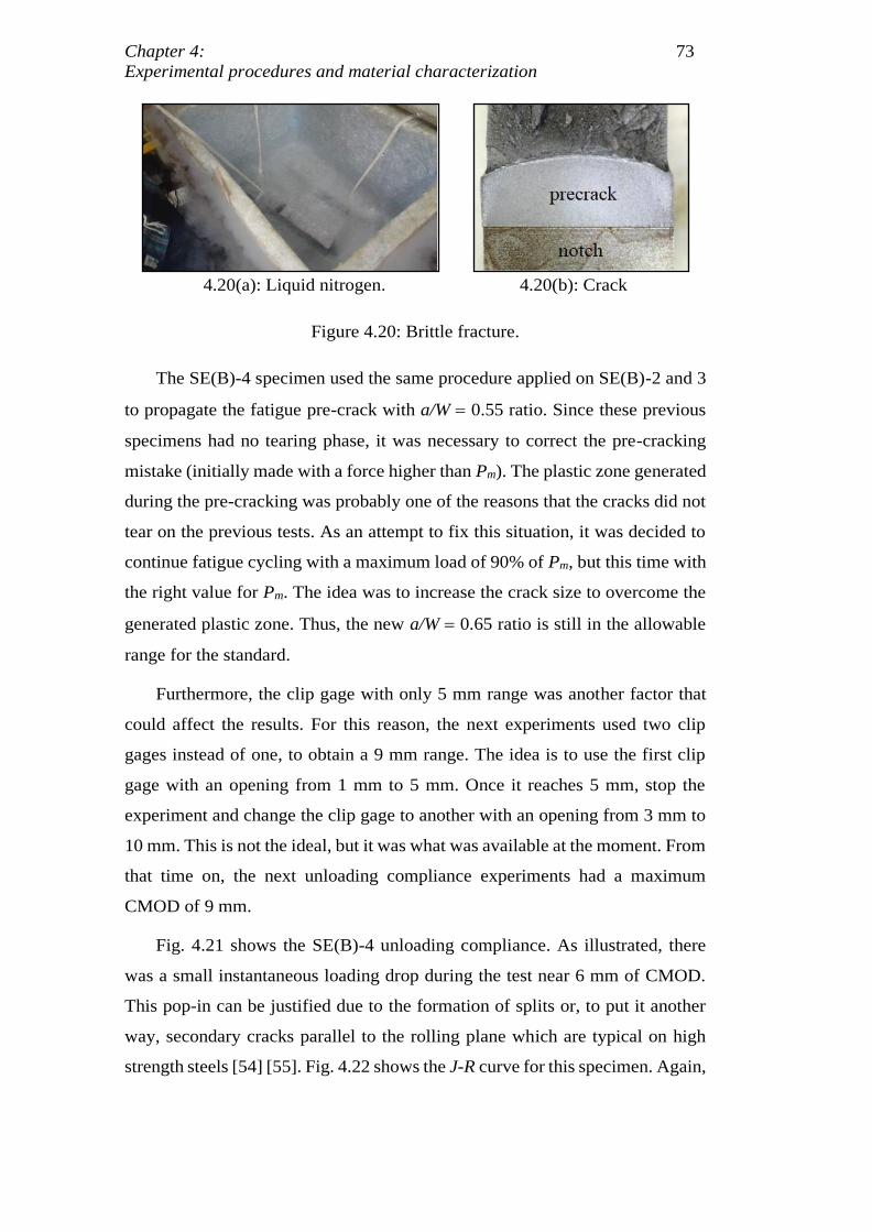
Chapter 4: 73


4.20(a): Liquid nitrogen. 4.20(b): Crack

Figure 4.20: Brittle fracture.

The SE(B)-4 specimen used the same procedure applied on SE(B)-2 and 3

to propagate the fatigue pre-crack with a/W = 0.55 ratio. Since these previous

specimens had no tearing phase, it was necessary to correct the pre-cracking

mistake (initially made with a force higher than Pm). The plastic zone generated

during the pre-cracking was probably one of the reasons that the cracks did not

tear on the previous tests. As an attempt to fix this situation, it was decided to

continue fatigue cycling with a maximum load of 90% of Pm, but this time with

the right value for Pm. The idea was to increase the crack size to overcome the

generated plastic zone. Thus, the new a/W = 0.65 ratio is still in the allowable

range for the standard.

Furthermore, the clip gage with only 5 mm range was another factor that

could affect the results. For this reason, the next experiments used two clip

gages instead of one, to obtain a 9 mm range. The idea is to use the first clip

gage with an opening from 1 mm to 5 mm. Once it reaches 5 mm, stop the

experiment and change the clip gage to another with an opening from 3 mm to

10 mm. This is not the ideal, but it was what was available at the moment. From

that time on, the next unloading compliance experiments had a maximum

CMOD of 9 mm.

Fig. 4.21 shows the SE(B)-4 unloading compliance. As illustrated, there

was a small instantaneous loading drop during the test near 6 mm of CMOD.

This pop-in can be justified due to the formation of splits or, to put it another

way, secondary cracks parallel to the rolling plane which are typical on high

strength steels [54] [55]. Fig. 4.22 shows the J-R curve for this specimen. Again,

DBD


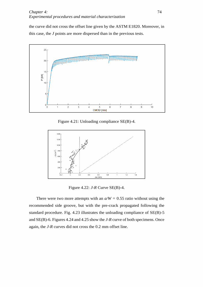
Chapter 4: 74


the curve did not cross the offset line given by the ASTM E1820. Moreover, in

this case, the J points are more dispersed than in the previous tests.

Figure 4.21: Unloading compliance SE(B)-4.

Figure 4.22: J-R Curve SE(B)-4.

There were two more attempts with an a/W = 0.55 ratio without using the

recommended side groove, but with the pre-crack propagated following the

standard procedure. Fig. 4.23 illustrates the unloading compliance of SE(B)-5

and SE(B)-6. Figures 4.24 and 4.25 show the J-R curve of both specimens. Once

again, the J-R curves did not cross the 0.2 mm offset line.

DBD


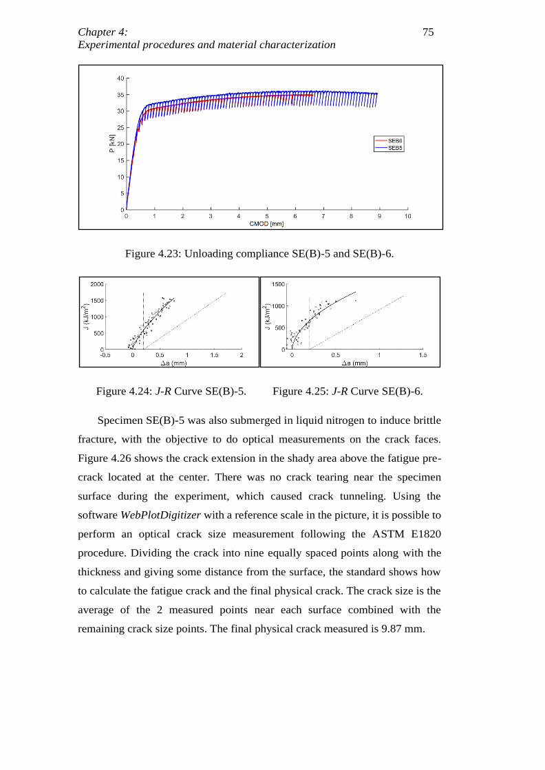
Chapter 4: 75




Specimen SE(B)-5 was also submerged in liquid nitrogen to induce brittle

fracture, with the objective to do optical measurements on the crack faces.

Figure 4.26 shows the crack extension in the shady area above the fatigue pre-

crack located at the center. There was no crack tearing near the specimen

surface during the experiment, which caused crack tunneling. Using the

software WebPlotDigitizer with a reference scale in the picture, it is possible to

perform an optical crack size measurement following the ASTM E1820

procedure. Dividing the crack into nine equally spaced points along with the

thickness and giving some distance from the surface, the standard shows how

to calculate the fatigue crack and the final physical crack. The crack size is the

average of the 2 measured points near each surface combined with the

remaining crack size points. The final physical crack measured is 9.87 mm.

DBD


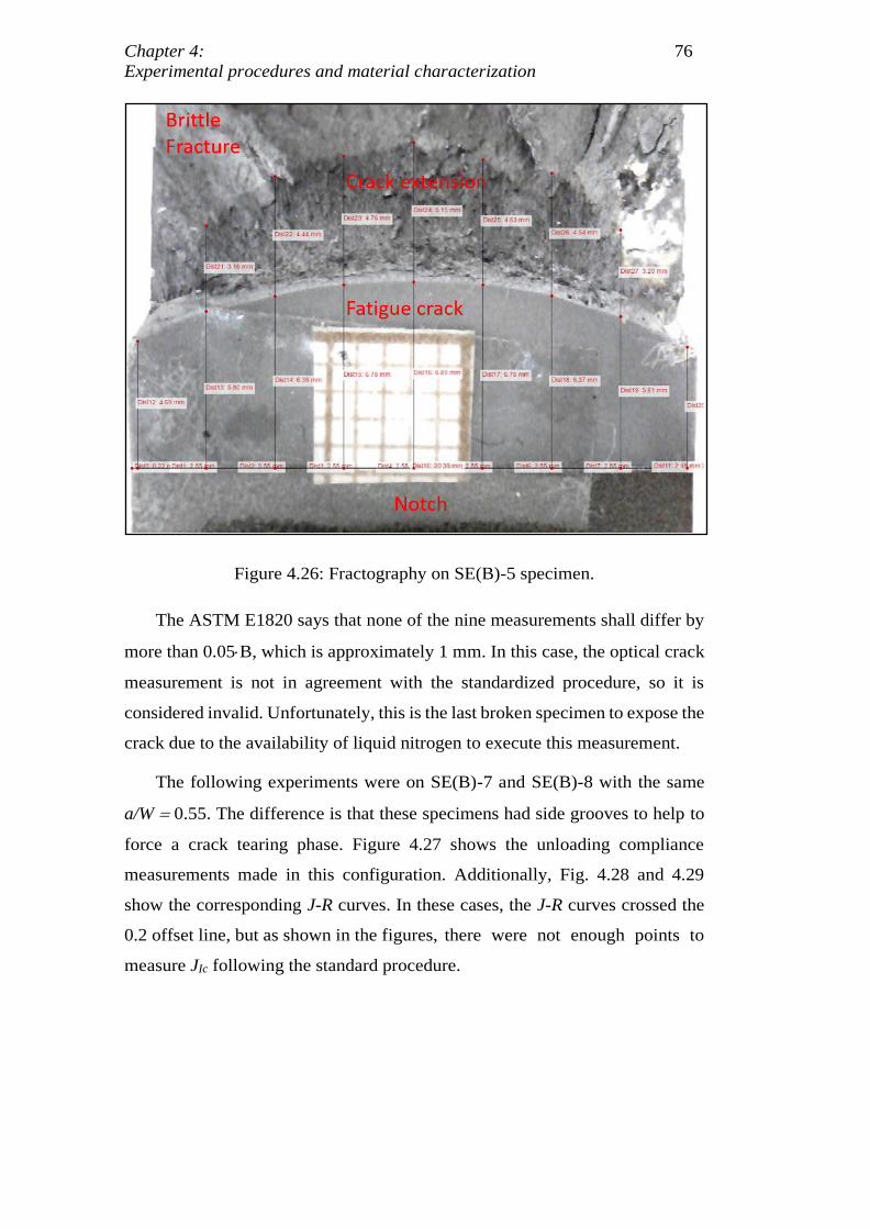
Chapter 4: 76


Figure 4.26: Fractography on SE(B)-5 specimen.

The ASTM E1820 says that none of the nine measurements shall differ by

more than 0.05B, which is approximately 1 mm. In this case, the optical crack

measurement is not in agreement with the standardized procedure, so it is

considered invalid. Unfortunately, this is the last broken specimen to expose the

crack due to the availability of liquid nitrogen to execute this measurement.

The following experiments were on SE(B)-7 and SE(B)-8 with the same

a/W = 0.55. The difference is that these specimens had side grooves to help to

force a crack tearing phase. Figure 4.27 shows the unloading compliance

measurements made in this configuration. Additionally, Fig. 4.28 and 4.29

show the corresponding J-R curves. In these cases, the J-R curves crossed the

0.2 offset line, but as shown in the figures, there were not enough points to

measure JIc following the standard procedure.

DBD


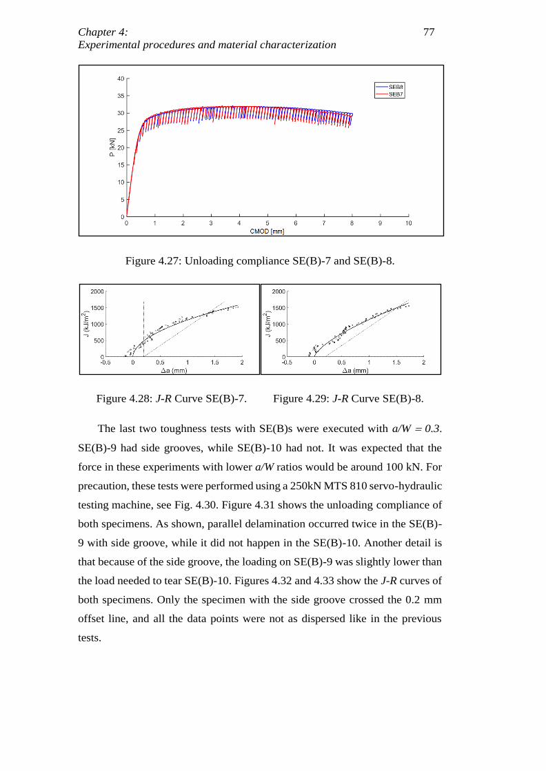
Chapter 4: 77




The last two toughness tests with SE(B)s were executed with a/W = 0.3.

SE(B)-9 had side grooves, while SE(B)-10 had not. It was expected that the

force in these experiments with lower a/W ratios would be around 100 kN. For

precaution, these tests were performed using a 250kN MTS 810 servo-hydraulic

testing machine, see Fig. 4.30. Figure 4.31 shows the unloading compliance of

both specimens. As shown, parallel delamination occurred twice in the SE(B)-

9 with side groove, while it did not happen in the SE(B)-10. Another detail is

that because of the side groove, the loading on SE(B)-9 was slightly lower than

the load needed to tear SE(B)-10. Figures 4.32 and 4.33 show the J-R curves of

both specimens. Only the specimen with the side groove crossed the 0.2 mm

offset line, and all the data points were not as dispersed like in the previous

tests.

DBD


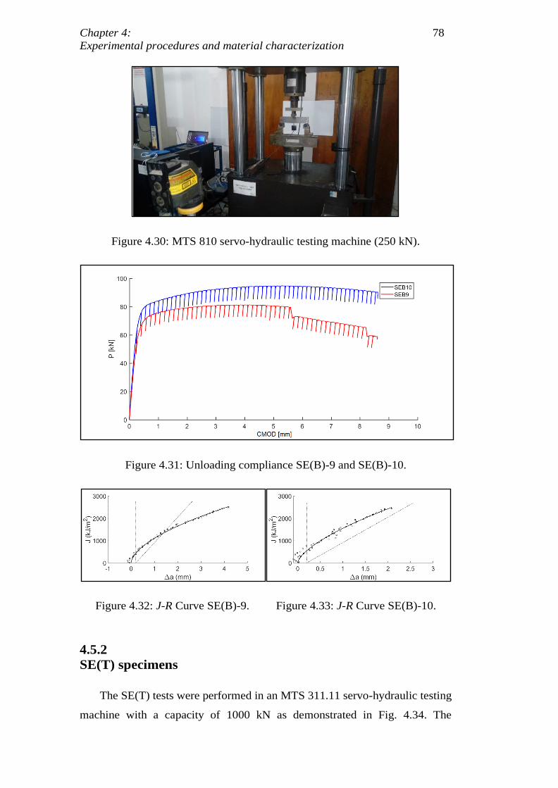
Chapter 4: 78


Figure 4.30: MTS 810 servo-hydraulic testing machine (250 kN).



4.5.2

SE(T) specimens

The SE(T) tests were performed in an MTS 311.11 servo-hydraulic testing

machine with a capacity of 1000 kN as demonstrated in Fig. 4.34. The

DBD


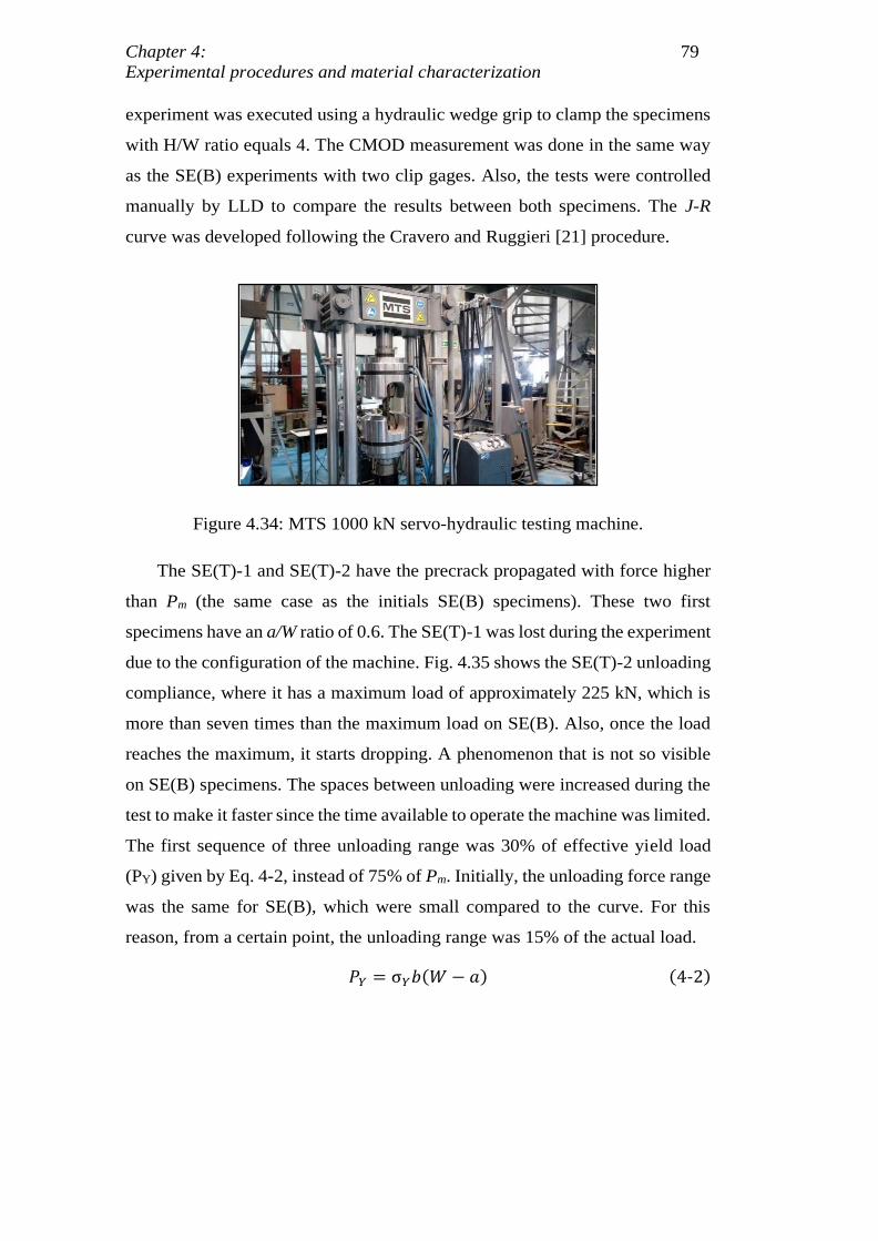
Chapter 4: 79


experiment was executed using a hydraulic wedge grip to clamp the specimens

with H/W ratio equals 4. The CMOD measurement was done in the same way

as the SE(B) experiments with two clip gages. Also, the tests were controlled

manually by LLD to compare the results between both specimens. The J-R

curve was developed following the Cravero and Ruggieri [21] procedure.

Figure 4.34: MTS 1000 kN servo-hydraulic testing machine.

The SE(T)-1 and SE(T)-2 have the precrack propagated with force higher

than Pm (the same case as the initials SE(B) specimens). These two first

specimens have an a/W ratio of 0.6. The SE(T)-1 was lost during the experiment

due to the configuration of the machine. Fig. 4.35 shows the SE(T)-2 unloading

compliance, where it has a maximum load of approximately 225 kN, which is

more than seven times than the maximum load on SE(B). Also, once the load

reaches the maximum, it starts dropping. A phenomenon that is not so visible

on SE(B) specimens. The spaces between unloading were increased during the

test to make it faster since the time available to operate the machine was limited.

The first sequence of three unloading range was 30% of effective yield load

(PY) given by Eq. 4-2, instead of 75% of Pm. Initially, the unloading force range

was the same for SE(B), which were small compared to the curve. For this

reason, from a certain point, the unloading range was 15% of the actual load.

𝑃𝑌 = σ𝑌𝑏(𝑊 − 𝑎) (4-2)

DBD


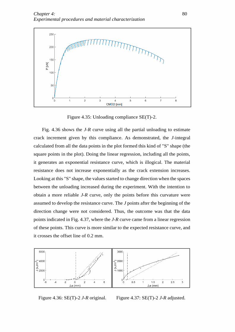
Chapter 4: 80


Figure 4.35: Unloading compliance SE(T)-2.

Fig. 4.36 shows the J-R curve using all the partial unloading to estimate

crack increment given by this compliance. As demonstrated, the J-integral

calculated from all the data points in the plot formed this kind of "S" shape (the

square points in the plot). Doing the linear regression, including all the points,

it generates an exponential resistance curve, which is illogical. The material

resistance does not increase exponentially as the crack extension increases.

Looking at this "S" shape, the values started to change direction when the spaces

between the unloading increased during the experiment. With the intention to

obtain a more reliable J-R curve, only the points before this curvature were

assumed to develop the resistance curve. The J points after the beginning of the

direction change were not considered. Thus, the outcome was that the data

points indicated in Fig. 4.37, where the J-R curve came from a linear regression

of these points. This curve is more similar to the expected resistance curve, and

it crosses the offset line of 0.2 mm.

Figure 4.36: SE(T)-2 J-R original. Figure 4.37: SE(T)-2 J-R adjusted.

DBD


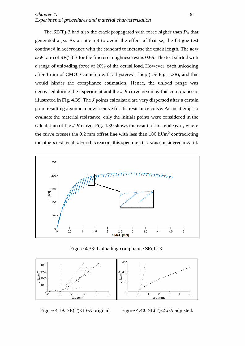
Chapter 4: 81


The SE(T)-3 had also the crack propagated with force higher than Pm that

generated a pz. As an attempt to avoid the effect of that pz, the fatigue test

continued in accordance with the standard to increase the crack length. The new

a/W ratio of SE(T)-3 for the fracture toughness test is 0.65. The test started with

a range of unloading force of 20% of the actual load. However, each unloading

after 1 mm of CMOD came up with a hysteresis loop (see Fig. 4.38), and this

would hinder the compliance estimation. Hence, the unload range was

decreased during the experiment and the J-R curve given by this compliance is

illustrated in Fig. 4.39. The J points calculated are very dispersed after a certain

point resulting again in a power curve for the resistance curve. As an attempt to

evaluate the material resistance, only the initials points were considered in the

calculation of the J-R curve. Fig. 4.39 shows the result of this endeavor, where

the curve crosses the 0.2 mm offset line with less than 100 kJ/m2 contradicting

the others test results. For this reason, this specimen test was considered invalid.



DBD


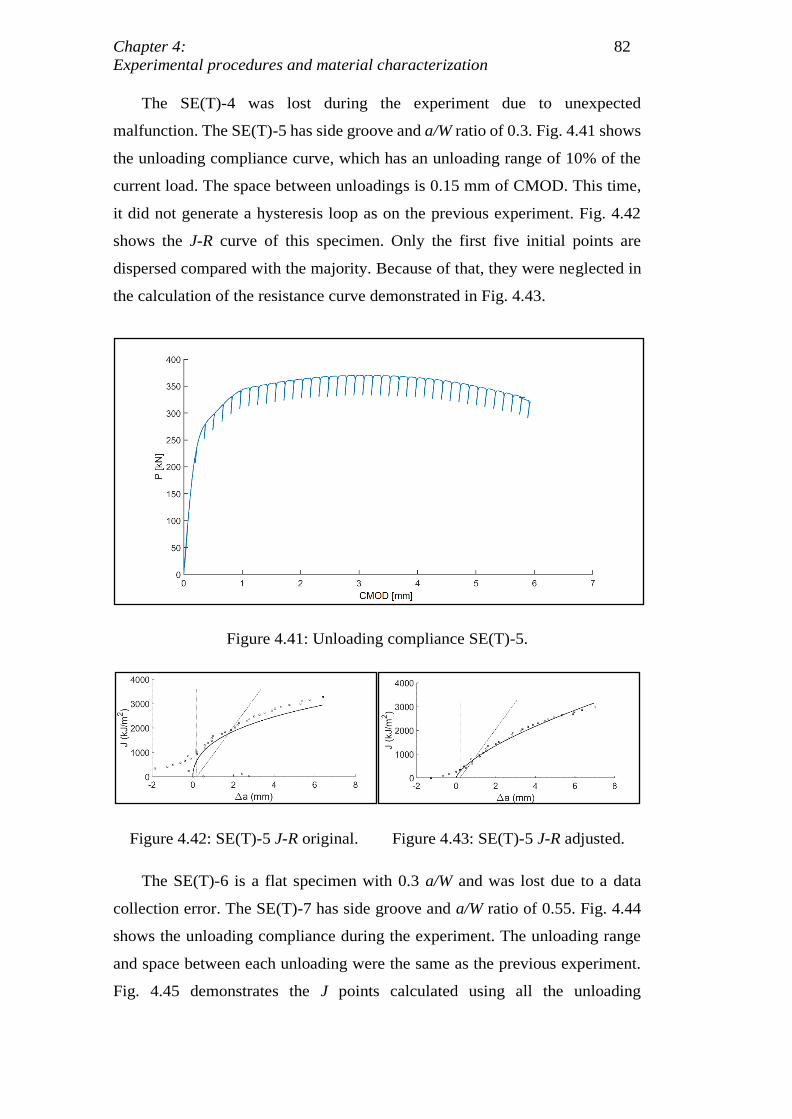
Chapter 4: 82


The SE(T)-4 was lost during the experiment due to unexpected

malfunction. The SE(T)-5 has side groove and a/W ratio of 0.3. Fig. 4.41 shows

the unloading compliance curve, which has an unloading range of 10% of the

current load. The space between unloadings is 0.15 mm of CMOD. This time,

it did not generate a hysteresis loop as on the previous experiment. Fig. 4.42

shows the J-R curve of this specimen. Only the first five initial points are

dispersed compared with the majority. Because of that, they were neglected in

the calculation of the resistance curve demonstrated in Fig. 4.43.



The SE(T)-6 is a flat specimen with 0.3 a/W and was lost due to a data

collection error. The SE(T)-7 has side groove and a/W ratio of 0.55. Fig. 4.44

shows the unloading compliance during the experiment. The unloading range

and space between each unloading were the same as the previous experiment.

Fig. 4.45 demonstrates the J points calculated using all the unloading

DBD


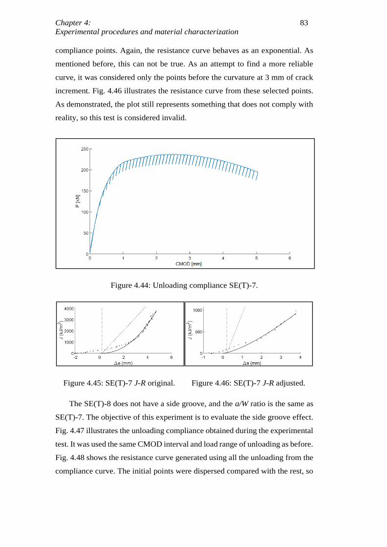
Chapter 4: 83


compliance points. Again, the resistance curve behaves as an exponential. As

mentioned before, this can not be true. As an attempt to find a more reliable

curve, it was considered only the points before the curvature at 3 mm of crack

increment. Fig. 4.46 illustrates the resistance curve from these selected points.

As demonstrated, the plot still represents something that does not comply with

reality, so this test is considered invalid.



The SE(T)-8 does not have a side groove, and the a/W ratio is the same as

SE(T)-7. The objective of this experiment is to evaluate the side groove effect.

Fig. 4.47 illustrates the unloading compliance obtained during the experimental

test. It was used the same CMOD interval and load range of unloading as before.

Fig. 4.48 shows the resistance curve generated using all the unloading from the

compliance curve. The initial points were dispersed compared with the rest, so

DBD


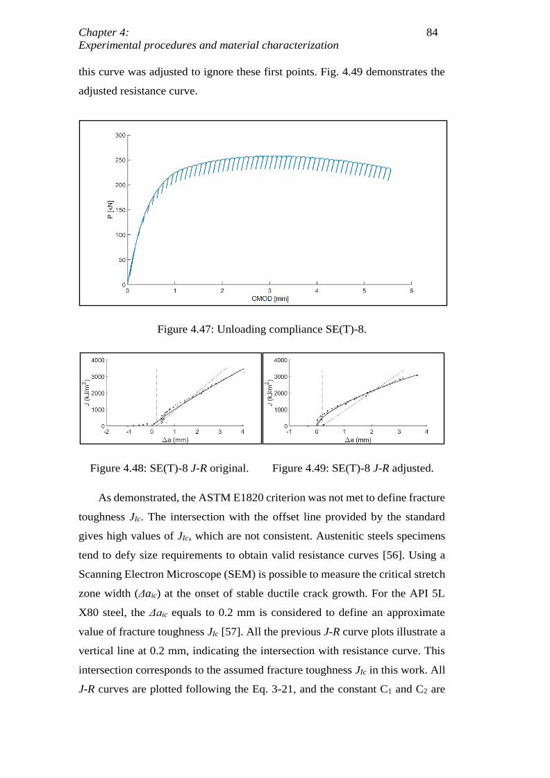
Chapter 4: 84


this curve was adjusted to ignore these first points. Fig. 4.49 demonstrates the

adjusted resistance curve.



As demonstrated, the ASTM E1820 criterion was not met to define fracture

toughness JIc. The intersection with the offset line provided by the standard

gives high values of JIc, which are not consistent. Austenitic steels specimens

tend to defy size requirements to obtain valid resistance curves [56]. Using a

Scanning Electron Microscope (SEM) is possible to measure the critical stretch

zone width (Δaic) at the onset of stable ductile crack growth. For the API 5L

X80 steel, the Δaic equals to 0.2 mm is considered to define an approximate

value of fracture toughness JIc [57]. All the previous J-R curve plots illustrate a

vertical line at 0.2 mm, indicating the intersection with resistance curve. This

intersection corresponds to the assumed fracture toughness JIc in this work. All

J-R curves are plotted following the Eq. 3-21, and the constant C1 and C2 are

DBD


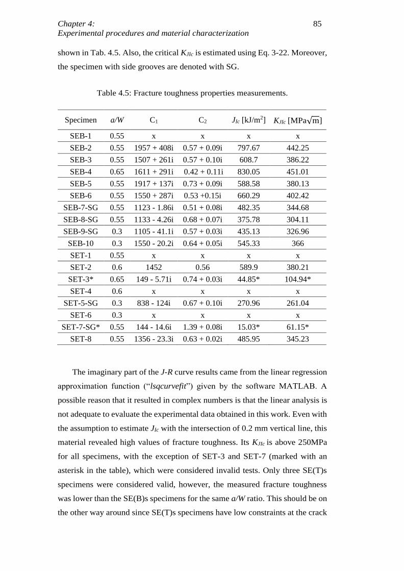
Chapter 4: 85


shown in Tab. 4.5. Also, the critical KJIc is estimated using Eq. 3-22. Moreover,

the specimen with side grooves are denoted with SG.

Table 4.5: Fracture toughness properties measurements.

Specimen a/W C1 C2 JIc [kJ/m2] KJIc [MPa√m]

SEB-1 0.55 x x x x

SEB-2 0.55 1957 + 408i 0.57 + 0.09i 797.67 442.25

SEB-3 0.55 1507 + 261i 0.57 + 0.10i 608.7 386.22

SEB-4 0.65 1611 + 291i 0.42 + 0.11i 830.05 451.01

SEB-5 0.55 1917 + 137i 0.73 + 0.09i 588.58 380.13

SEB-6 0.55 1550 + 287i 0.53 +0.15i 660.29 402.42

SEB-7-SG 0.55 1123 - 1.86i 0.51 + 0.08i 482.35 344.68

SEB-8-SG 0.55 1133 - 4.26i 0.68 + 0.07i 375.78 304.11

SEB-9-SG 0.3 1105 - 41.1i 0.57 + 0.03i 435.13 326.96

SEB-10 0.3 1550 - 20.2i 0.64 + 0.05i 545.33 366

SET-1 0.55 x x x x

SET-2 0.6 1452 0.56 589.9 380.21

SET-3* 0.65 149 - 5.71i 0.74 + 0.03i 44.85* 104.94*

SET-4 0.6 x x x x

SET-5-SG 0.3 838 - 124i 0.67 + 0.10i 270.96 261.04

SET-6 0.3 x x x x

SET-7-SG* 0.55 144 - 14.6i 1.39 + 0.08i 15.03* 61.15*

SET-8 0.55 1356 - 23.3i 0.63 + 0.02i 485.95 345.23

The imaginary part of the J-R curve results came from the linear regression

approximation function (“lsqcurvefit”) given by the software MATLAB. A

possible reason that it resulted in complex numbers is that the linear analysis is

not adequate to evaluate the experimental data obtained in this work. Even with

the assumption to estimate JIc with the intersection of 0.2 mm vertical line, this

material revealed high values of fracture toughness. Its KJIc is above 250MPa

for all specimens, with the exception of SET-3 and SET-7 (marked with an

asterisk in the table), which were considered invalid tests. Only three SE(T)s

specimens were considered valid, however, the measured fracture toughness

was lower than the SE(B)s specimens for the same a/W ratio. This should be on

the other way around since SE(T)s specimens have low constraints at the crack

DBD


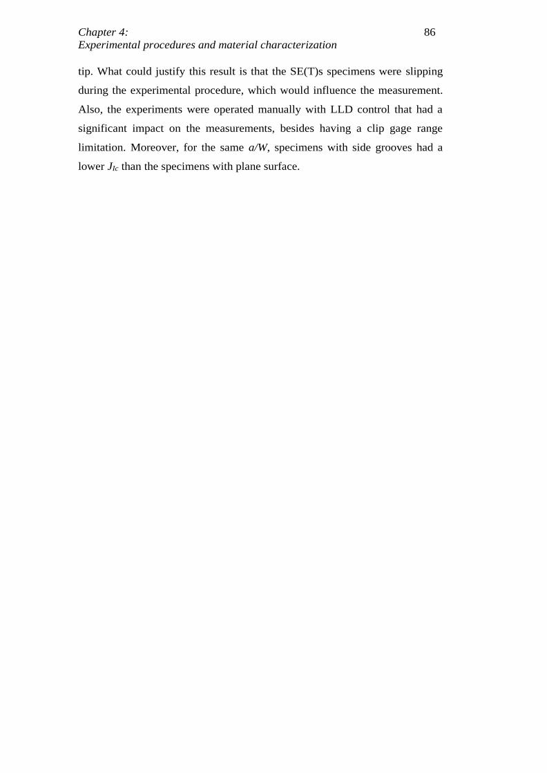
Chapter 4: 86


tip. What could justify this result is that the SE(T)s specimens were slipping

during the experimental procedure, which would influence the measurement.

Also, the experiments were operated manually with LLD control that had a

significant impact on the measurements, besides having a clip gage range

limitation. Moreover, for the same a/W, specimens with side grooves had a

lower JIc than the specimens with plane surface.

DBD


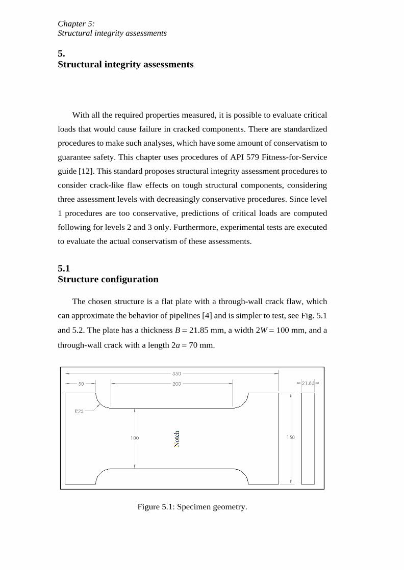
Chapter 5:

Structural integrity assessments

5.


With all the required properties measured, it is possible to evaluate critical

loads that would cause failure in cracked components. There are standardized

procedures to make such analyses, which have some amount of conservatism to

guarantee safety. This chapter uses procedures of API 579 Fitness-for-Service

guide [12]. This standard proposes structural integrity assessment procedures to

consider crack-like flaw effects on tough structural components, considering

three assessment levels with decreasingly conservative procedures. Since level

1 procedures are too conservative, predictions of critical loads are computed

following for levels 2 and 3 only. Furthermore, experimental tests are executed

to evaluate the actual conservatism of these assessments.

5.1

Structure configuration

The chosen structure is a flat plate with a through-wall crack flaw, which

can approximate the behavior of pipelines [4] and is simpler to test, see Fig. 5.1

and 5.2. The plate has a thickness B = 21.85 mm, a width 2W = 100 mm, and a

through-wall crack with a length 2a = 70 mm.

Figure 5.1: Specimen geometry.

DBD


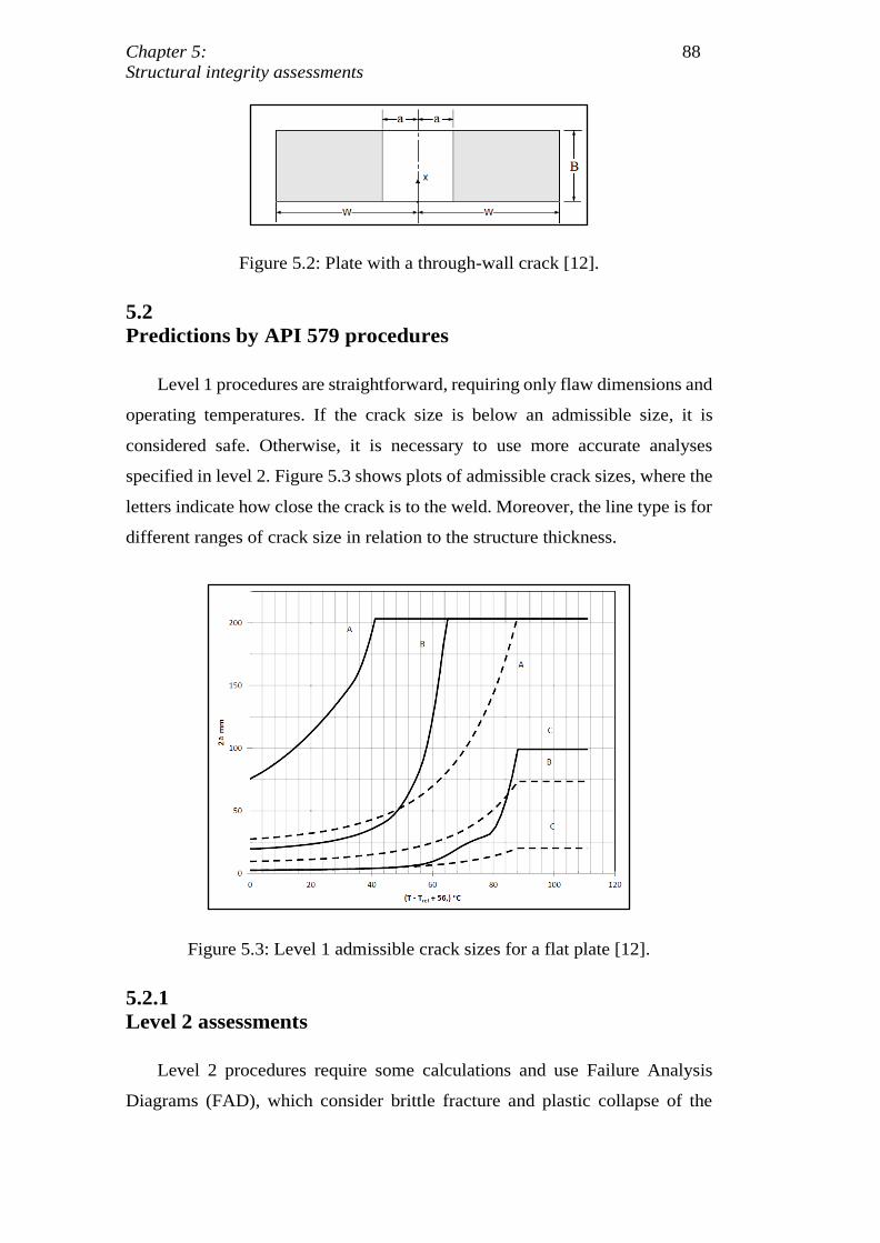
Chapter 5: 88


Figure 5.2: Plate with a through-wall crack [12].

5.2

Predictions by API 579 procedures

Level 1 procedures are straightforward, requiring only flaw dimensions and

operating temperatures. If the crack size is below an admissible size, it is

considered safe. Otherwise, it is necessary to use more accurate analyses

specified in level 2. Figure 5.3 shows plots of admissible crack sizes, where the

letters indicate how close the crack is to the weld. Moreover, the line type is for

different ranges of crack size in relation to the structure thickness.

Figure 5.3: Level 1 admissible crack sizes for a flat plate [12].

5.2.1

Level 2 assessments

Level 2 procedures require some calculations and use Failure Analysis

Diagrams (FAD), which consider brittle fracture and plastic collapse of the

DBD


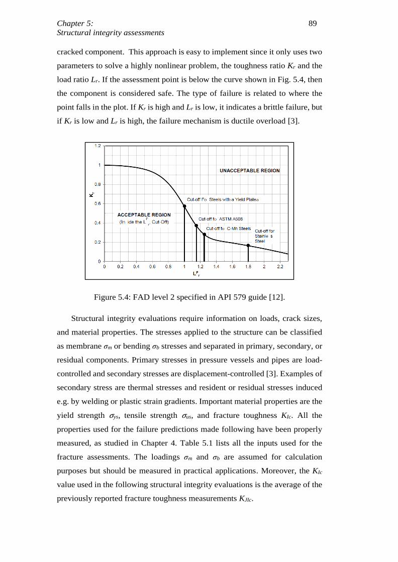
Chapter 5: 89


cracked component. This approach is easy to implement since it only uses two

parameters to solve a highly nonlinear problem, the toughness ratio Kr and the

load ratio Lr. If the assessment point is below the curve shown in Fig. 5.4, then

the component is considered safe. The type of failure is related to where the

point falls in the plot. If Kr is high and Lr is low, it indicates a brittle failure, but

if Kr is low and Lr is high, the failure mechanism is ductile overload [3].

Figure 5.4: FAD level 2 specified in API 579 guide [12].

Structural integrity evaluations require information on loads, crack sizes,

and material properties. The stresses applied to the structure can be classified

as membrane σm or bending σb stresses and separated in primary, secondary, or

residual components. Primary stresses in pressure vessels and pipes are load-

controlled and secondary stresses are displacement-controlled [3]. Examples of

secondary stress are thermal stresses and resident or residual stresses induced

e.g. by welding or plastic strain gradients. Important material properties are the

yield strength σys, tensile strength σus, and fracture toughness KIc. All the

properties used for the failure predictions made following have been properly

measured, as studied in Chapter 4. Table 5.1 lists all the inputs used for the

fracture assessments. The loadings σm and σb are assumed for calculation

purposes but should be measured in practical applications. Moreover, the KIc

value used in the following structural integrity evaluations is the average of the

previously reported fracture toughness measurements KJIc.

DBD


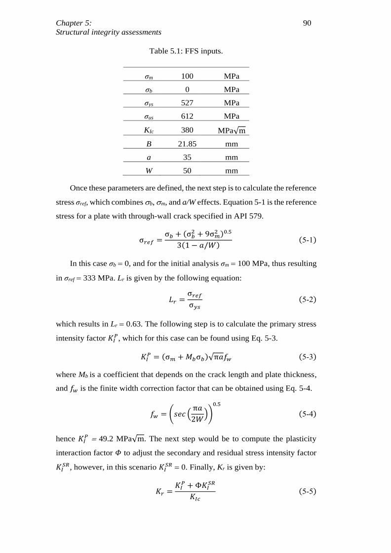
Chapter 5: 90


Table 5.1: FFS inputs.

σm 100 MPa

σb 0 MPa

σys 527 MPa

σus 612 MPa

KIc 380 MPa√m

B 21.85 mm

a 35 mm

W 50 mm

Once these parameters are defined, the next step is to calculate the reference

stress σref, which combines b, m, and a/W effects. Equation 5-1 is the reference

stress for a plate with through-wall crack specified in API 579.

σ𝑟𝑒𝑓 =σ𝑏 + (σ𝑏

2 + 9σ𝑚2 )0.5

3(1 − 𝑎/𝑊)(5-1)

In this case σb = 0, and for the initial analysis σm = 100 MPa, thus resulting

in σref = 333 MPa. Lr is given by the following equation:

𝐿𝑟 =σ𝑟𝑒𝑓

σ𝑦𝑠

(5-2)

which results in Lr = 0.63. The following step is to calculate the primary stress

intensity factor 𝐾𝐼𝑃, which for this case can be found using Eq. 5-3.

𝐾𝐼𝑃 = (σ𝑚 + 𝑀𝑏σ𝑏)√π𝑎𝑓𝑤 (5-3)

where Mb is a coefficient that depends on the crack length and plate thickness,

and 𝑓𝑤 is the finite width correction factor that can be obtained using Eq. 5-4.

𝑓𝑤 = (𝑠𝑒𝑐 (π𝑎

2𝑊))

0.5

(5-4)

hence 𝐾𝐼𝑃 = 49.2 MPa√m. The next step would be to compute the plasticity

interaction factor 𝛷 to adjust the secondary and residual stress intensity factor

𝐾𝐼𝑆𝑅, however, in this scenario 𝐾𝐼

𝑆𝑅 = 0. Finally, Kr is given by:

𝐾𝑟 =𝐾𝐼

𝑃 + Φ𝐾𝐼𝑆𝑅

𝐾𝐼𝑐

(5-5)

DBD


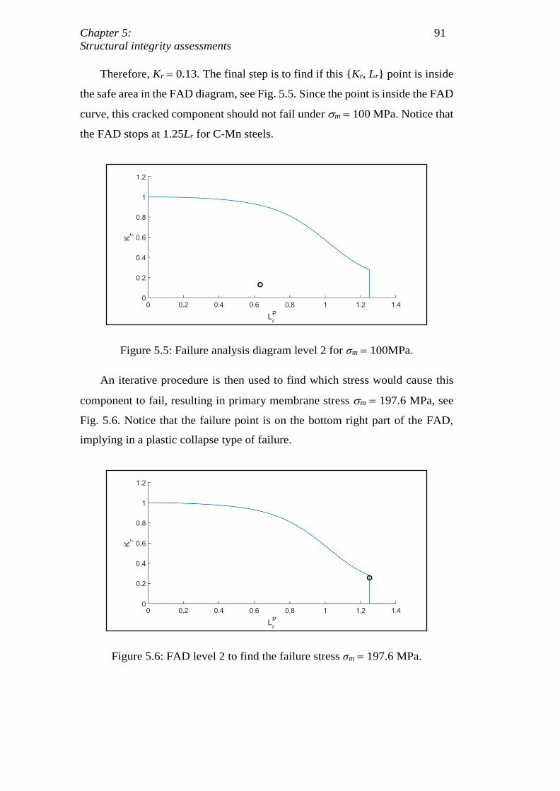
Chapter 5: 91


Therefore, Kr = 0.13. The final step is to find if this {Kr, Lr} point is inside

the safe area in the FAD diagram, see Fig. 5.5. Since the point is inside the FAD

curve, this cracked component should not fail under m = 100 MPa. Notice that

the FAD stops at 1.25Lr for C-Mn steels.

Figure 5.5: Failure analysis diagram level 2 for σm = 100MPa.

An iterative procedure is then used to find which stress would cause this

component to fail, resulting in primary membrane stress m = 197.6 MPa, see

Fig. 5.6. Notice that the failure point is on the bottom right part of the FAD,

implying in a plastic collapse type of failure.

Figure 5.6: FAD level 2 to find the failure stress σm = 197.6 MPa.

DBD


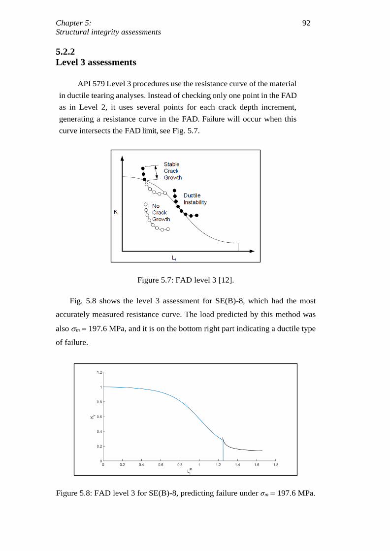
Chapter 5: 92


5.2.2

Level 3 assessments

API 579 Level 3 procedures use the resistance curve of the material

in ductile tearing analyses. Instead of checking only one point in the FAD

as in Level 2, it uses several points for each crack depth increment,

generating a resistance curve in the FAD. Failure will occur when this

curve intersects the FAD limit, see Fig. 5.7.

Figure 5.7: FAD level 3 [12].

Fig. 5.8 shows the level 3 assessment for SE(B)-8, which had the most

accurately measured resistance curve. The load predicted by this method was

also m = 197.6 MPa, and it is on the bottom right part indicating a ductile type

of failure.

Figure 5.8: FAD level 3 for SE(B)-8, predicting failure under σm = 197.6 MPa.

DBD


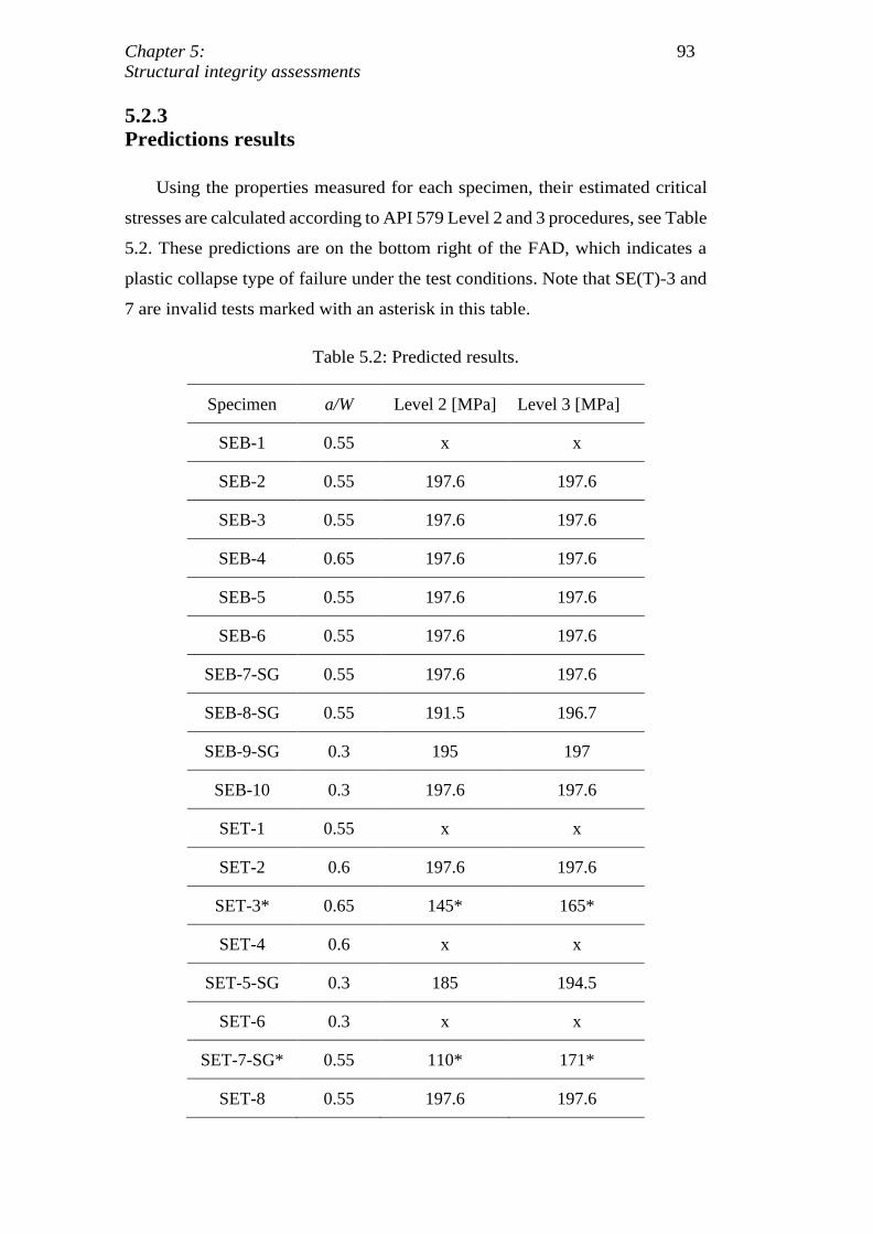
Chapter 5: 93


5.2.3

Predictions results

Using the properties measured for each specimen, their estimated critical

stresses are calculated according to API 579 Level 2 and 3 procedures, see Table

5.2. These predictions are on the bottom right of the FAD, which indicates a

plastic collapse type of failure under the test conditions. Note that SE(T)-3 and

7 are invalid tests marked with an asterisk in this table.

Table 5.2: Predicted results.

Specimen a/W Level 2 [MPa] Level 3 [MPa]

SEB-1 0.55 x x

SEB-2 0.55 197.6 197.6

SEB-3 0.55 197.6 197.6

SEB-4 0.65 197.6 197.6

SEB-5 0.55 197.6 197.6

SEB-6 0.55 197.6 197.6

SEB-7-SG 0.55 197.6 197.6

SEB-8-SG 0.55 191.5 196.7

SEB-9-SG 0.3 195 197

SEB-10 0.3 197.6 197.6

SET-1 0.55 x x

SET-2 0.6 197.6 197.6

SET-3* 0.65 145* 165*

SET-4 0.6 x x

SET-5-SG 0.3 185 194.5

SET-6 0.3 x x

SET-7-SG* 0.55 110* 171*

SET-8 0.55 197.6 197.6

DBD


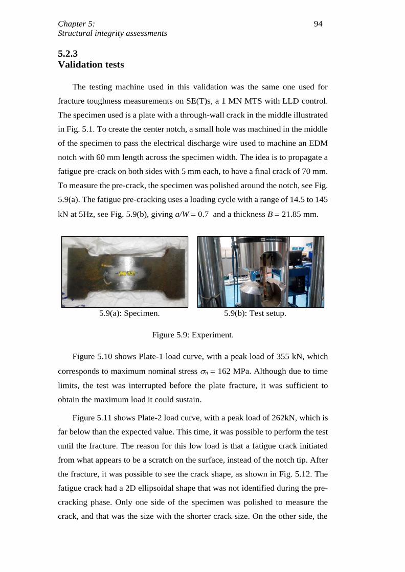
Chapter 5: 94


5.2.3

Validation tests

The testing machine used in this validation was the same one used for

fracture toughness measurements on SE(T)s, a 1 MN MTS with LLD control.

The specimen used is a plate with a through-wall crack in the middle illustrated

in Fig. 5.1. To create the center notch, a small hole was machined in the middle

of the specimen to pass the electrical discharge wire used to machine an EDM

notch with 60 mm length across the specimen width. The idea is to propagate a

fatigue pre-crack on both sides with 5 mm each, to have a final crack of 70 mm.

To measure the pre-crack, the specimen was polished around the notch, see Fig.

5.9(a). The fatigue pre-cracking uses a loading cycle with a range of 14.5 to 145

kN at 5Hz, see Fig. 5.9(b), giving a/W = 0.7 and a thickness B = 21.85 mm.

5.9(a): Specimen. 5.9(b): Test setup.

Figure 5.9: Experiment.

Figure 5.10 shows Plate-1 load curve, with a peak load of 355 kN, which

corresponds to maximum nominal stress n = 162 MPa. Although due to time

limits, the test was interrupted before the plate fracture, it was sufficient to

obtain the maximum load it could sustain.

Figure 5.11 shows Plate-2 load curve, with a peak load of 262kN, which is

far below than the expected value. This time, it was possible to perform the test

until the fracture. The reason for this low load is that a fatigue crack initiated

from what appears to be a scratch on the surface, instead of the notch tip. After

the fracture, it was possible to see the crack shape, as shown in Fig. 5.12. The

fatigue crack had a 2D ellipsoidal shape that was not identified during the pre-

cracking phase. Only one side of the specimen was polished to measure the

crack, and that was the size with the shorter crack size. On the other side, the

DBD


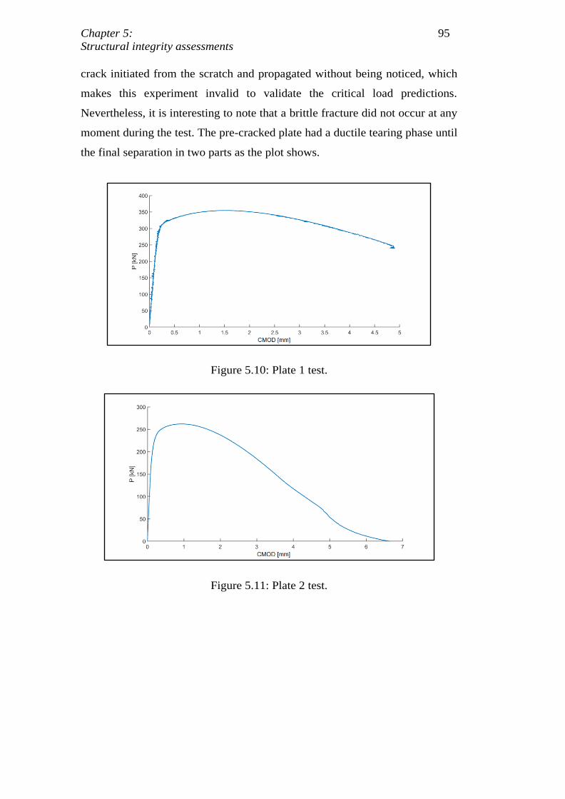
Chapter 5: 95


crack initiated from the scratch and propagated without being noticed, which

makes this experiment invalid to validate the critical load predictions.

Nevertheless, it is interesting to note that a brittle fracture did not occur at any

moment during the test. The pre-cracked plate had a ductile tearing phase until

the final separation in two parts as the plot shows.

Figure 5.10: Plate 1 test.

Figure 5.11: Plate 2 test.

DBD


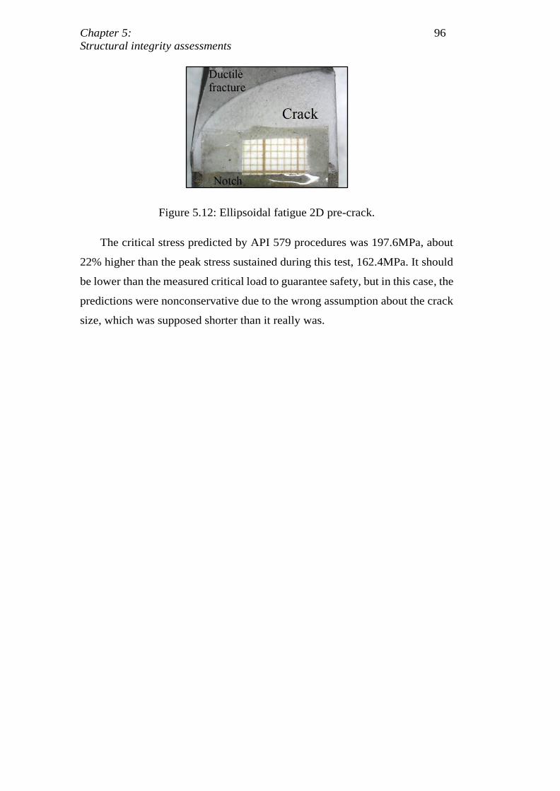
Chapter 5: 96


Figure 5.12: Ellipsoidal fatigue 2D pre-crack.

The critical stress predicted by API 579 procedures was 197.6MPa, about

22% higher than the peak stress sustained during this test, 162.4MPa. It should

be lower than the measured critical load to guarantee safety, but in this case, the

predictions were nonconservative due to the wrong assumption about the crack

size, which was supposed shorter than it really was.

DBD


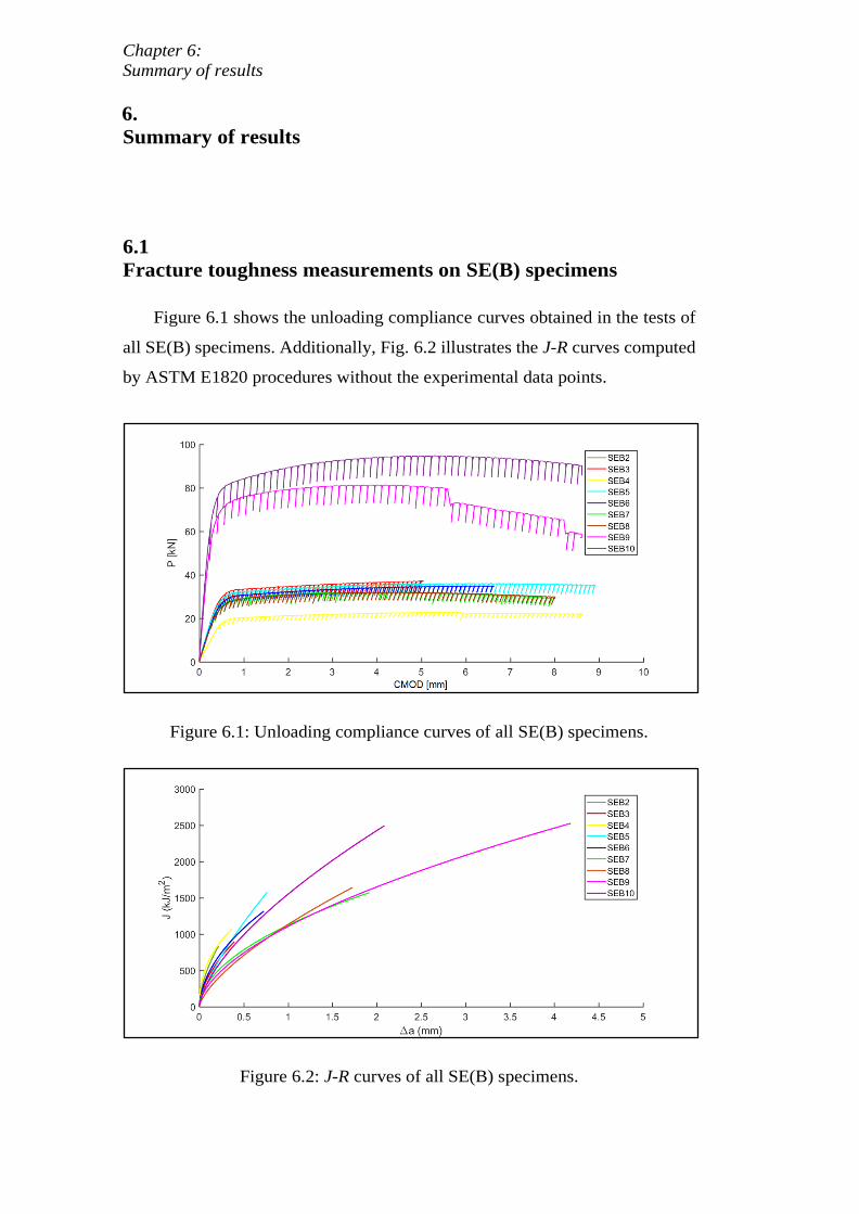
Chapter 6:

Summary of results

6.

Summary of results

6.1

Fracture toughness measurements on SE(B) specimens

Figure 6.1 shows the unloading compliance curves obtained in the tests of

all SE(B) specimens. Additionally, Fig. 6.2 illustrates the J-R curves computed

by ASTM E1820 procedures without the experimental data points.

Figure 6.1: Unloading compliance curves of all SE(B) specimens.

Figure 6.2: J-R curves of all SE(B) specimens.

DBD


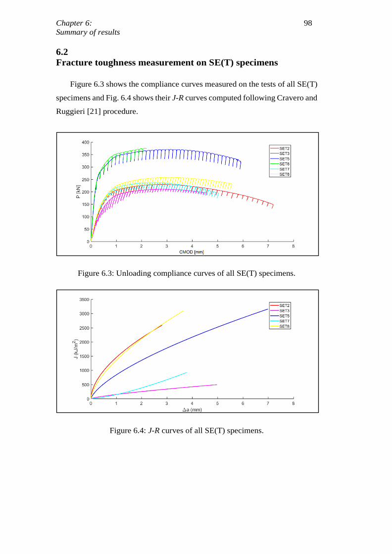
Chapter 6: 98

Summary of results

6.2

Fracture toughness measurement on SE(T) specimens

Figure 6.3 shows the compliance curves measured on the tests of all SE(T)

specimens and Fig. 6.4 shows their J-R curves computed following Cravero and

Ruggieri [21] procedure.

Figure 6.3: Unloading compliance curves of all SE(T) specimens.

Figure 6.4: J-R curves of all SE(T) specimens.

DBD


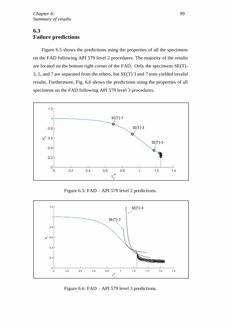
Chapter 6: 99

Summary of results

6.3

Failure predictions

Figure 6.5 shows the predictions using the properties of all the specimens

on the FAD following API 579 level 2 procedures. The majority of the results

are located on the bottom right corner of the FAD. Only the specimens SE(T)-

3, 5, and 7 are separated from the others, but SE(T) 3 and 7 tests yielded invalid

results. Furthermore, Fig. 6.6 shows the predictions using the properties of all

specimens on the FAD following API 579 level 3 procedures.

Figure 6.5: FAD – API 579 level 2 predictions.

Figure 6.6: FAD – API 579 level 3 predictions.

DBD


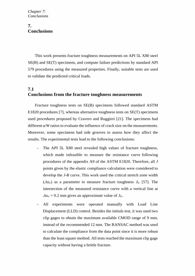
Chapter 7:

Conclusions

7.

Conclusions

This work presents fracture toughness measurements on API 5L X80 steel

SE(B) and SE(T) specimens, and compute failure predictions by standard API

579 procedures using the measured properties. Finally, suitable tests are used

to validate the predicted critical loads.

7.1

Conclusions from the fracture toughness measurements

Fracture toughness tests on SE(B) specimens followed standard ASTM

E1820 procedures [7], whereas alternative toughness tests on SE(T) specimens

used procedures proposed by Cravero and Ruggieri [21]. The specimens had

different a/W ratios to evaluate the influence of crack size on the measurements.

Moreover, some specimens had side grooves to assess how they affect the

results. The experimental tests lead to the following conclusions:

- The API 5L X80 steel revealed high values of fracture toughness,

which made infeasible to measure the resistance curve following

procedures of the appendix A9 of the ASTM E1820. Therefore, all J

points given by the elastic compliance calculation were considered to

develop the J-R curve. This work used the critical stretch zone width

(Δaic) as a parameter to measure fracture toughness JIc [57]. The

intersection of the measured resistance curve with a vertical line at

Δaic = 0.2 mm gives an approximate value of JIc.

- All experiments were operated manually with Load Line

Displacement (LLD) control. Besides the initials test, it was used two

clip gages to obtain the maximum available CMOD range of 9 mm,

instead of the recommended 12 mm. The RANSAC method was used

to calculate the compliance from the data point since it is more robust

than the least square method. All tests reached the maximum clip gage

capacity without having a brittle fracture.

DBD


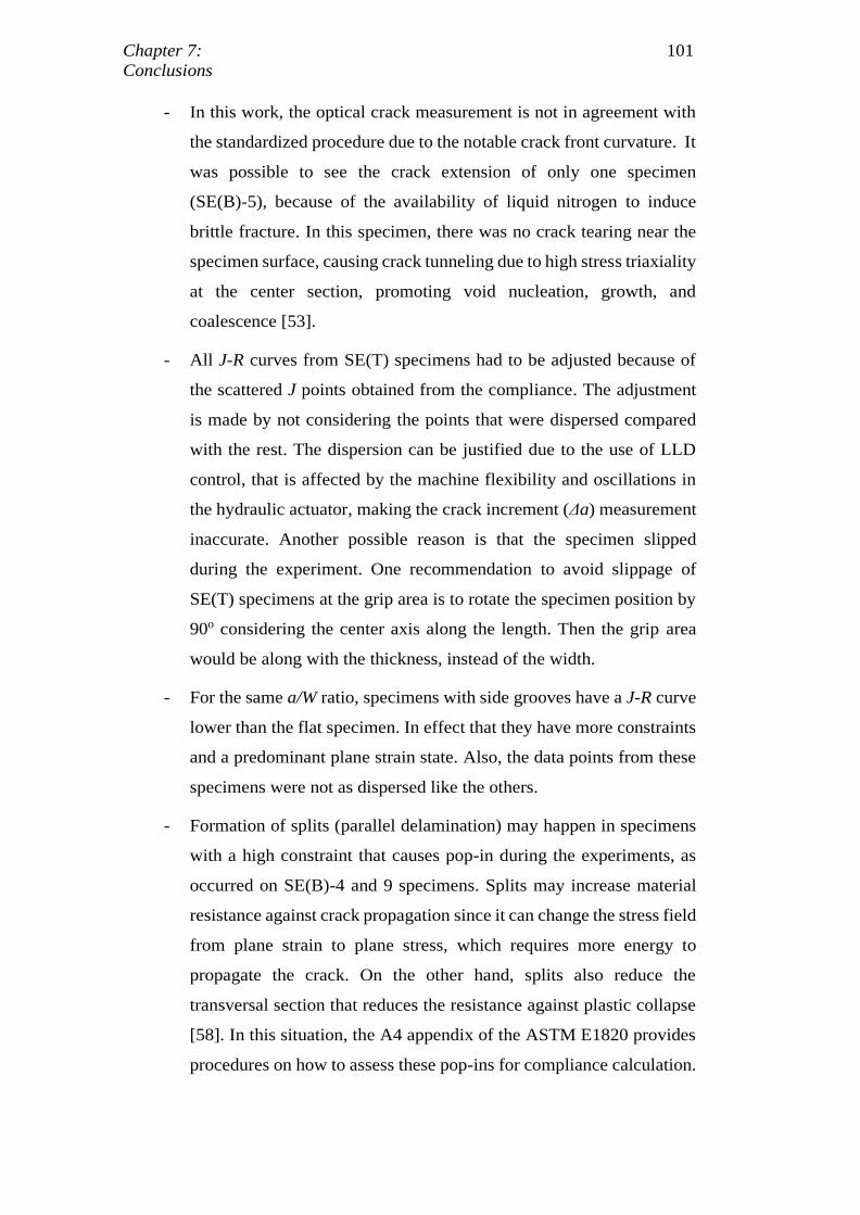
Chapter 7: 101

Conclusions

- In this work, the optical crack measurement is not in agreement with

the standardized procedure due to the notable crack front curvature. It

was possible to see the crack extension of only one specimen

(SE(B)-5), because of the availability of liquid nitrogen to induce

brittle fracture. In this specimen, there was no crack tearing near the

specimen surface, causing crack tunneling due to high stress triaxiality

at the center section, promoting void nucleation, growth, and

coalescence [53].

- All J-R curves from SE(T) specimens had to be adjusted because of

the scattered J points obtained from the compliance. The adjustment

is made by not considering the points that were dispersed compared

with the rest. The dispersion can be justified due to the use of LLD

control, that is affected by the machine flexibility and oscillations in

the hydraulic actuator, making the crack increment (Δa) measurement

inaccurate. Another possible reason is that the specimen slipped

during the experiment. One recommendation to avoid slippage of

SE(T) specimens at the grip area is to rotate the specimen position by

90o considering the center axis along the length. Then the grip area

would be along with the thickness, instead of the width.

- For the same a/W ratio, specimens with side grooves have a J-R curve

lower than the flat specimen. In effect that they have more constraints

and a predominant plane strain state. Also, the data points from these

specimens were not as dispersed like the others.

- Formation of splits (parallel delamination) may happen in specimens

with a high constraint that causes pop-in during the experiments, as

occurred on SE(B)-4 and 9 specimens. Splits may increase material

resistance against crack propagation since it can change the stress field

from plane strain to plane stress, which requires more energy to

propagate the crack. On the other hand, splits also reduce the

transversal section that reduces the resistance against plastic collapse

[58]. In this situation, the A4 appendix of the ASTM E1820 provides

procedures on how to assess these pop-ins for compliance calculation.

DBD


Chapter 7: 102

Conclusions

- As expected, the SE(T) specimens were able to support higher loads

than the SE(B) specimens. Also, once the load reaches the maximum

for SE(T) specimens, it starts dropping. A phenomenon that did not

occur on SE(B) specimens.

7.2

Conclusions from the failure predictions

Failure predictions followed procedures of the API 579 [12] levels 2 and 3

using the properties measured for each specimen. Moreover, the results were

compared with experimental tests using a plate specimen with a through-wall

crack in the middle.

- Most of the predictions are the same for level 2 and 3 of the API 579

since the toughness ratio and load ratio point {Kr, Lr} are located on

the bottom right of the Failure Analysis Diagram (FAD), which

indicates ductile failure. In this work, the API 5L X80 steel failure

mechanism is plastic collapse.

- Only two tests were performed, which one was considered invalid

since the fatigue crack initiated from a scratch on the surface instead

of the notch tip. Because of that, the crack size used for the predictions

is different from the crack at the specimen. Even with a/W ratio of

0.70, brittle fracture did not occur at any moment during the

experiment. The pre-cracked plate had a ductile tearing phase until the

final separation in two parts.

- All predictions following the API 579 procedure were higher than the

maximum stress obtained from the experiment, resulting in

nonconservative predictions. A possible reason for that is due to

inaccurate properties measurement. Another is the chosen FAD is not

adequate for high toughness materials. It is worth noting that only one

valid experiment was executed to make this evaluation, which is not

recommended. Unfortunately, it was not possible to perform more

tests due to time limit.

DBD


Chapter 7: 103

Conclusions

- On FAD level 2 and 3 only the prediction using SET-5 (a/W = 0.30)

properties is separated from the other predictions. All predictions

using SE(B) measurements have approximately the same result.

- As discussed, the API 5L X80 is very suitable steel for pipelines which

can withstand cracks in the base metal. Therefore, the critical region

that could occur fracture is at the welding section.

7.3

Recommendations for future work

- Measure the fracture toughness on C(T) specimens to compare with

the J-R curve results from SE(B).

- Execute more experiments with cracked plates to evaluate the

predictions made by the API 579 standard.

- Apply the structural integrity procedure on the welding and evaluate

the effect of the heat-affected zone (HAZ).

DBD


Bibliography

Bibliography

[1] BROEK, D. Elementary engineering fracture mechanics, Springer

Science and Business Media, 2012.

[2] HERTZBERG, R.W. Deformation and fracture mechanics of

engineering materials, Wiley, 1989.

[3] ANDERSON, T.L. Fracture mechanics: fundamentals and applications,

CRC press, 2017.

[4] CASTRO, J.T.P.D.; MEGGIOLARO, M.A. Fadiga: técnicas e práticas

de dimensionamento estrutural sob cargas reais de serviço: Volume I,II,

CreateSpace, 2009.

[5] ASTM E399, Standard Test Method for Linear-Elastic Plane-Strain

Fracture Toughness KIC of Metallic Materials, 2012.

[6] ASTM E1290, Standard Test Method for Crack-Tip Opening

Displacement (CTOD) Fracture Toughness Measurement, 2008.

[7] ASTM E1820-17a, Standard test method for measurement of fracture

toughness, 2017.

[8] BS 7448, Fracture Mechanics Toughness Tests. Method for

Determination of Kic, Critical CTOD and Critical J Values of

Metallic Materials, ISE British Standard, 1991.

[9] GKSS-RESEARCH, The GKSS Procedure for Determining the

Fracture Behavior of Materials., EFAM-GTP 02, 2002.

DBD


Bibliography 105

[10] LINK, R.E. Round-robin Analysis of Standard Data Sets for Fracture

Toughness Evaluation in ASTM E1820, Journal of Testing and

Evaluation, 2014.

[11] VERITAS, N. D. Fracture control for pipeline installation methods

introducing cyclic plastic strain, Recommended Practice DNV-RP-

F108, 2006.

[12] API 579-1/ASME FFS-1, Fitness-For-Service guide, 2016.

[13] HARRISON, R.; LOOSEMORE, K.; MILINE, I. Assessment of the

integrity of structure containing defects, Int. J. Pressure Vessel and

Piping, 1988.

[14] DILLSTRÖM, P.; BERGMAN, M. A combined deterministic and

probabilistic procedure for safety assessment of components with

cracks--Handbook, SSM report, 2008.

[15] WALLIN, K.; NEVASMAA, P. Structural Integrity Assessment

Procedures for European Industry (SINTAP), Sub-Task, 1997.

[16] BS 7910, Guide to methods for assessing the acceptability of flaws in

metallic structures, British Standard and others, 2015.

[17] Umm Said LPG Plant Disaster, [Online]. Available:

<https://pt.scribd.com/doc/21090127/UMM-Said-LPG-Plant-Disaster-

03-04-77>.

[18] Alexander L. Kielland platform capsize accident–investigation,

[Online]. Available: <https://officerofthewatch.com/2013/04/29/

alexander-l-kielland-platform-capsize-accident>.

[19] SS Schenectady, [Online]. Available: <https://en.wikipedia.org

/wiki/SS-Schenectady/>.

DBD


Bibliography 106

[20] Common Comet Misconceptions and Collaborative Contribution to

Safety, [Online].Available: <http://aerossurance.com/safety-management

/ comet-misconceptions/>.

[21] CRAVERO S.; RUGGIERI, C. Estimation procedure of J-resistance

curves for SE (T) fracture specimens using unloading compliance,

Engineering Fracture Mechanics, 2007.

[22] PEDROSA, I.R.V. et al. Study of phase transformations In API 5L X80

Steel in order to increase its fracture toughness, Materials Research,

2013.

[23] BHADESHIA, H.; HONEYCOMBE, R. Steels: microstructure and

properties, 2017.

[24] ASTM E8/E8M - 16a, Standard Test Methods for Tension Testing of

Metallic Materials, 2016.

[25] LIU, A.F. Mechanics and mechanisms of fracture: an introduction,

ASM International, 2005.

[26] HANDROK, J.L.; COMER, J.J.; BANNANTINE, J.A. Fundamentals of

Metal Fatigue Analysis, Prentice Hall, 1990

[27] CHEN, R.C.J.H. Micromechanism of Cleavage Fracture of Metals,

Elsevier Inc., 2015.

[28] MEDINA, J.A.H. Avaliação de Previsões de Fraturas Elastoplásticas,

PUC-Rio, 2014.

[29] MAITI, S. K. Fracture Mechanics, Cambridge University Press, 2015.

[30] BURDEKIN, F.; DAWES, M. Practical use of linear elastic and

yielding fracture mechanics with particular reference to pressure

DBD


Bibliography 107

vessels, Proceedings of the Institute of Mechanical Engineers Conference,

1971.

[31] HUTCHINSON, J. Singular behaviour at the end of a tensile crack in

a hardening material, Journal of the Mechanics and Physics of Solids,

1968.

[32] RICE, J. Plane strain deformation near a crack tip in a power-law

hardening material, Journal of the Mechanics and Physics of Solids,

1968.

[33] KIRK, M. T.; KOPPENHOEFER, K. C.; SHIH, C. F. Effect of constraint

on specimen dimensions needed to obtain structurally relevant

toughness measures, Constraint effects in fracture, 1993.

[34] SHIH, C.; GERMAN, M. Requirements for a one parameter

characterization of crack tip fields by the HRR singularity,

International Journal of Fracture, 1981.

[35] BETEGON, C.; HANCOCK, J. Two-parameter characterization of

elastic-plastic crack-tip fields, Journal of applied mechanics, 1991.

[36] O'DOWD, N.; SHIH, C. F. Family of crack-tip fields characterized by

a triaxiality parameter—I. Structure of fields, Journal of the Mechanics

and Physics of Solids, 1991.

[37] O'DOWD, N.; SHIH, C. F. Family of crack-tip fields characterized by

a triaxiality parameter—II. Fracture applications, Journal of the

Mechanics and Physics of Solids, 1992.

[38] SHEN, G. et al. Measurement of JR curves using single-specimen

technique on clamped SE (T) specimens, The Nineteenth International

Offshore and Polar Engineering Conference, 2009.

DBD


Bibliography 108

[39] KANG, J. et al. Influence of Constraint on J-resistance Curves for an

X100 Pipe Steel, Procedia materials science, 2014.

[40] CHIESA, M. et al. Efficient fracture assessment of pipelines. A

constraint-corrected SENT specimen approach, Engineering Fracture

Mechanics, 2001.

[41] WILLIAMS, M. L. The bending stress distribution at the base of a

stationary crack, Journal of applied mechanics, 1961.

[42] YASUFUMI, I.; TOMOKAZU, M. Effect of side grooves on the elastic-

plastic stress state of fracture toughness specimens—three-

dimensional finite element analysis, Engineering Fracture Mechanics,

1982.

[43] ANDREWS, W.; SHIH, C. Thickness and side-groove effects on J-and

δ-resistance curves for A533-B steel at 93° C, Elastic-plastic fracture,

1979.

[44] JOYCE, J.A. Manual on elastic-plastic fracture: laboratory text

procedures, 1996.

[45] SHEN, G.; GIANETTO, J.; TYSON, W. Development of procedure for

low-constraint toughness testing using a single-specimen technique,

CANMET Materials Technology Laboratory, Technical Report, 2008.

[46] CIRINO, J. et al. Caracterização microestrutural do aço API 5L X80

em amostras sumetidas a diferentes ataques quimicos.

[47] ZHOU, M. et al. Microstructure characteristics and mechanical

properties of X80 pipeline steels, Journal of Wuhan University of

Technology-Mater. Sci. Ed., 2012.

[48] USIMINAS; CONFAB; PETROBRÁS; CEFET-RJ; PUC-RJ, Estudos

de aplicações do aço x80 para tubos, Programa Nacional de Ciência e

DBD


Bibliography 109

Tecnologia do Setor de Petróleo e Gás Natural – CTPETRO: Projeto

cooperativo Universidade-Empresa, 2002.

[49] AMERICAN PETROLEUM INSTITUTE, API5L Specification for line

pipe steel, 43th, 2004.

[50] DIN 50150, Conversion of hardness values for metallic materials,

2000.

[51] JOO, M. S. et al. Mechanical anisotropy in steels for pipelines, ISIJ

international, 2013.

[52] FISCHLER, M.; BOLLES, R. Random sample consensus: a paradigm

for model fitting with applications to image analysis and automated

cartography, Commum ACM, 24:381, 1981.

[53] LAN, W.; DENG, X.; SUTTON, M.A. Investigation of crack tunneling

in ductile materials, Engineering Fracture Mechanics, 2010.

[54] ARNOULT, X. et al. Short review: Potential impact of delamination

cracks on fracture toughness of structural materials, Frattura ed Integrita

Strutturale, 2016.

[55] SILVA, M.D.C. Caracterização das propriedades mecânicas e

metaúrgicas do aço API 5L X80 e determinação experimental de

curvas JR para avaliação da tenacidade a fratura, 2016.

[56] SCHWALBE, K.H.; CORNEC, A.; BAUSTIAN, K. Application of

fracture mechanics Principles to austenitic steels, International journal

of pressure vessels and piping, 1996.

[57] ZHU, X.K.; LEIS, B.N. Application of constraint corrected JR curves

to fracture analysis of pipelines, Journal of Pressure Vessel Technology,

2006.

DBD


Bibliography 110

[58] HIPPERT JUNIOR, E. Investigação expeirmental do comportamento

dúctiol de aços API-x70 e aplicação de curvas de resitência J-Δa para

previsão de colapso em dutos, Escola Politécnica, Universidade de São

Paulo, 2004.

DBD


Eduardo Enes Cota Toughness Evaluation and Fracture ...

Documents

Transcript of Eduardo Enes Cota Toughness Evaluation and Fracture ...