Editorial Board S. Axler K.A. Ribet · x Acknowledgments Roman Shvidkoy, Elias Stein, Atanas...

Graduate Texts in Mathematics 249

Editorial BoardS. Axler

K.A. Ribet

Graduate Texts in Mathematics1 TAKEUTI/ZARING. Introduction to Axiomatic

Set Theory. 2nd ed.2 OXTOBY. Measure and Category. 2nd ed.3 SCHAEFER. Topological Vector Spaces.

2nd ed.4 HILTON/STAMMBACH. A Course in

Homological Algebra. 2nd ed.5 MAC LANE. Categories for the Working

Mathematician. 2nd ed.6 HUGHES/PIPER. Projective Planes.7 J.-P. SERRE. A Course in Arithmetic.8 TAKEUTI/ZARING. Axiomatic Set Theory.9 HUMPHREYS. Introduction to Lie Algebras

and Representation Theory.10 COHEN. A Course in Simple Homotopy

Theory.11 CONWAY. Functions of One Complex

Variable I. 2nd ed.12 BEALS. Advanced Mathematical Analysis.13 ANDERSON/FULLER. Rings and Categories

of Modules. 2nd ed.14 GOLUBITSKY/GUILLEMIN. Stable Mappings

and Their Singularities.15 BERBERIAN. Lectures in Functional Analysis

and Operator Theory.16 WINTER. The Structure of Fields.17 ROSENBLATT. Random Processes. 2nd ed.18 HALMOS. Measure Theory.19 HALMOS. A Hilbert Space Problem Book.

2nd ed.20 HUSEMOLLER. Fibre Bundles. 3rd ed.21 HUMPHREYS. Linear Algebraic Groups.22 BARNES/MACK. An Algebraic Introduction

to Mathematical Logic.23 GREUB. Linear Algebra. 4th ed.24 HOLMES. Geometric Functional Analysis and

Its Applications.25 HEWITT/STROMBERG. Real and Abstract

Analysis.26 MANES. Algebraic Theories.27 KELLEY. General Topology.28 ZARISKI/SAMUEL.CommutativeAlgebra.

Vol. I.29 ZARISKI/SAMUEL. Commutative Algebra.

Vol. II.30 JACOBSON. Lectures in Abstract Algebra I.

Basic Concepts.31 JACOBSON. Lectures in Abstract Algebra II.

Linear Algebra.32 JACOBSON. Lectures in Abstract Algebra III.

Theory of Fields and Galois Theory.33 HIRSCH. Differential Topology.34 SPITZER. Principles of Random Walk. 2nd ed.35 ALEXANDER/WERMER. Several Complex

Variables and Banach Algebras. 3rd ed.36 KELLEY/NAMIOKA ET AL. Linear

Topological Spaces.37 MONK. Mathematical Logic.

38 GRAUERT/FRITZSCHE. Several ComplexVariables.

39 ARVESON. An Invitation to C-Algebras.40 KEMENY/SNELL/KNAPP. Denumerable

Markov Chains. 2nd ed.41 APOSTOL. Modular Functions and Dirichlet

Series in Number Theory. 2nd ed.42 J.-P. SERRE. Linear Representations of Finite

Groups.43 GILLMAN/JERISON. Rings of Continuous

Functions.44 KENDIG. Elementary Algebraic Geometry.45 LOEVE. Probability Theory I. 4th ed.46 LOEVE. Probability Theory II. 4th ed.47 MOISE. Geometric Topology in Dimensions 2

and 3.48 SACHS/WU. General Relativity for

Mathematicians.49 GRUENBERG/WEIR. Linear Geometry.

2nd ed.50 EDWARDS. Fermat’s Last Theorem.51 KLINGENBERG. A Course in Differential

Geometry.52 HARTSHORNE. Algebraic Geometry.53 MANIN. A Course in Mathematical Logic.54 GRAVER/WATKINS. Combinatorics with

Emphasis on the Theory of Graphs.55 BROWN/PEARCY. Introduction to Operator

Theory I: Elements of Functional Analysis.56 MASSEY. Algebraic Topology: An

Introduction.57 CROWELL/FOX. Introduction to Knot Theory.58 KOBLITZ. p-adic Numbers, p-adic Analysis,

and Zeta-Functions. 2nd ed.59 LANG. Cyclotomic Fields.60 ARNOLD. Mathematical Methods in Classical

Mechanics. 2nd ed.61 WHITEHEAD. Elements of Homotopy Theory.62 KARGAPOLOV/MERIZJAKOV. Fundamentals

of the Theory of Groups.63 BOLLOBAS. Graph Theory.64 EDWARDS. Fourier Series. Vol. I. 2nd ed.65 WELLS. Differential Analysis on Complex

Manifolds. 2nd ed.66 WATERHOUSE. Introduction to Affine Group

Schemes.67 SERRE. Local Fields.68 WEIDMANN. Linear Operators in Hilbert

Spaces.69 LANG. Cyclotomic Fields II.70 MASSEY. Singular Homology Theory.71 FARKAS/KRA. Riemann Surfaces. 2nd ed.72 STILLWELL. Classical Topology and

Combinatorial Group Theory. 2nd ed.73 HUNGERFORD. Algebra.74 DAVENPORT. Multiplicative Number Theory.

3rd ed.(continued after index)

Classical Fourier Analysis

Second Edition

Loukas Grafakos

123

springer.com

Loukas Grafakos

Editorial Board

S. AxlerMathematics DepartmentSan Francisco State UniversitySan Francisco, CA [email protected]

K.A. RibetMathematics DepartmentUniversity of California at BerkeleyBerkeley, CA [email protected]

Library of Congress Control Number: 2008933456

Mathematics Subject Classifi cation (2000): 42-xx 42-02

© 2008 Springer Science+Business Media, LLCAll rights reserved. This work may not be translated or copied in whole or in part without the written permission of the publisher (Springer Science+Business Media, LLC, 233 Spring Street, New York, NY 10013, USA), except for brief excerpts in connection with reviews or scholarly analysis. Use in connection with any form of information storage and retrieval, electronic adaptation, computer software, or by similar or dissimilar methodology now known or hereafter developed is forbidden.The use in this publication of trade names, trademarks, service marks, and similar terms, even if they are not identifi ed as such, is not to be taken as an expression of opinion as to whether or not they are subject to proprietary rights.

Printed on acid-free paper

ISBN: 978-0-387-09431-1 e-ISBN: 978-0-387-09432-8DOI: 10.1007/978-0-387-09432-8

ISSN: 0072-5285

University of Missouri

[email protected]

Columbia, MO 65211USA

Department of Mathematics

To Suzanne

Preface

The great response to the publication of the book Classical and Modern FourierAnalysis has been very gratifying. I am delighted that Springer has offered to publishthe second edition of this book in two volumes: Classical Fourier Analysis, 2ndEdition, and Modern Fourier Analysis, 2nd Edition.

These volumes are mainly addressed to graduate students who wish to studyFourier analysis. This first volume is intended to serve as a text for a one-semestercourse in the subject. The prerequisite for understanding the material herein is satis-factory completion of courses in measure theory, Lebesgue integration, and complexvariables.

The details included in the proofs make the exposition longer. Although it willbehoove many readers to skim through the more technical aspects of the presenta-tion and concentrate on the flow of ideas, the fact that details are present will becomforting to some. The exercises at the end of each section enrich the materialof the corresponding section and provide an opportunity to develop additional intu-ition and deeper comprehension. The historical notes of each chapter are intended toprovide an account of past research but also to suggest directions for further investi-gation. The appendix includes miscellaneous auxiliary material needed throughoutthe text.

A web site for the book is maintained at

http://math.missouri.edu/∼loukas/FourierAnalysis.html

I am solely responsible for any misprints, mistakes, and historical omissions inthis book. Please contact me directly ([email protected]) if you have cor-rections, comments, suggestions for improvements, or questions.

Columbia, Missouri, Loukas GrafakosApril 2008

vii

Acknowledgments

I am very fortunate that several people have pointed out errors, misprints, and omis-sions in the first edition of this book. Others have clarified issues I raised concerningthe material it contains. All these individuals have provided me with invaluable helpthat resulted in the improved exposition of the present second edition. For thesereasons, I would like to express my deep appreciation and sincere gratitude to thefollowing people:

Marco Annoni, Pascal Auscher, Andrew Bailey, Dmitriy Bilyk, Marcin Bownik,Leonardo Colzani, Simon Cowell, Mita Das, Geoffrey Diestel, Yong Ding, JacekDziubanski, Wei He, Petr Honzık, Heidi Hulsizer, Philippe Jaming, Svante Janson,Ana Jimenez del Toro, John Kahl, Cornelia Kaiser, Nigel Kalton, Kim Jin My-ong, Doowon Koh, Elena Koutcherik, Enrico Laeng, Sungyun Lee, Qifan Li, Chin-Cheng Lin, Liguang Liu, Stig-Olof Londen, Diego Maldonado, Jose Marıa Martell,Mieczyslaw Mastylo, Parasar Mohanty, Carlo Morpurgo, Andrew Morris, MihailMourgoglou, Virginia Naibo, Hiro Oh, Marco Peloso, Maria Cristina Pereyra,Carlos Perez, Humberto Rafeiro, Maria Carmen Reguera Rodrıguez, AlexanderSamborskiy, Andreas Seeger, Steven Senger, Sumi Seo, Christopher Shane, ShuShen, Yoshihiro Sawano, Vladimir Stepanov, Erin Terwilleger, Rodolfo Torres,Suzanne Tourville, Ignacio Uriarte-Tuero, Kunyang Wang, Huoxiong Wu, TakashiYamamoto, and Dachun Yang.

For their valuable suggestions, corrections, and other important assistance at dif-ferent stages in the preparation of the first edition of this book, I would like to offermy deepest gratitude to the following individuals:

Georges Alexopoulos, Nakhle Asmar, Bruno Calado, Carmen Chicone, DavidCramer, Geoffrey Diestel, Jakub Duda, Brenda Frazier, Derrick Hart, Mark Hoff-mann, Steven Hofmann, Helge Holden, Brian Hollenbeck, Petr Honzık, AlexanderIosevich, Tunde Jakab, Svante Janson, Ana Jimenez del Toro, Gregory Jones, NigelKalton, Emmanouil Katsoprinakis, Dennis Kletzing, Steven Krantz, Douglas Kurtz,George Lobell, Xiaochun Li, Jose Marıa Martell, Antonios Melas, Keith Mers-man, Stephen Montgomety-Smith, Andrea Nahmod, Nguyen Cong Phuc, KrzysztofOleszkiewicz, Cristina Pereyra, Carlos Perez, Daniel Redmond, Jorge Rivera-Nori-ega, Dmitriy Ryabogin, Christopher Sansing, Lynn Savino Wendel, Shih-Chi Shen,

ix

x Acknowledgments

Roman Shvidkoy, Elias Stein, Atanas Stefanov, Terence Tao, Erin Terwilleger,Christoph Thiele, Rodolfo Torres, Deanie Tourville, Nikolaos Tzirakis Don Vaught,Igor Verbitsky, Brett Wick, James Wright, and Linqiao Zhao.

I would also like to thank all reviewers who provided me with an abundanceof meaningful remarks, corrections, and suggestions for improvements. Finally, Iwould like to thank Springer editor Mark Spencer, Springer’s digital product supportpersonnel Frank Ganz and Frank McGuckin, and copyeditor David Kramer for theirinvaluable assistance during the preparation of this edition.

Contents

1 Lp Spaces and Interpolation . . . . . . . . . . . . . . . . . . . . . . . . . . . . . . . . . . . . . 11.1 Lp and Weak Lp . . . . . . . . . . . . . . . . . . . . . . . . . . . . . . . . . . . . . . . . . . . . 1

1.1.1 The Distribution Function . . . . . . . . . . . . . . . . . . . . . . . . . . . . . 21.1.2 Convergence in Measure . . . . . . . . . . . . . . . . . . . . . . . . . . . . . . 51.1.3 A First Glimpse at Interpolation . . . . . . . . . . . . . . . . . . . . . . . . 8

Exercises . . . . . . . . . . . . . . . . . . . . . . . . . . . . . . . . . . . . . . . . . . . 101.2 Convolution and Approximate Identities . . . . . . . . . . . . . . . . . . . . . . . 16

1.2.1 Examples of Topological Groups . . . . . . . . . . . . . . . . . . . . . . . 161.2.2 Convolution . . . . . . . . . . . . . . . . . . . . . . . . . . . . . . . . . . . . . . . . . 181.2.3 Basic Convolution Inequalities . . . . . . . . . . . . . . . . . . . . . . . . . 191.2.4 Approximate Identities . . . . . . . . . . . . . . . . . . . . . . . . . . . . . . . 24

Exercises . . . . . . . . . . . . . . . . . . . . . . . . . . . . . . . . . . . . . . . . . . . 281.3 Interpolation . . . . . . . . . . . . . . . . . . . . . . . . . . . . . . . . . . . . . . . . . . . . . . . 30

1.3.1 Real Method: The Marcinkiewicz Interpolation Theorem . . . 311.3.2 Complex Method: The Riesz–Thorin Interpolation Theorem 341.3.3 Interpolation of Analytic Families of Operators . . . . . . . . . . . 371.3.4 Proofs of Lemmas 1.3.5 and 1.3.8 . . . . . . . . . . . . . . . . . . . . . . 39

Exercises . . . . . . . . . . . . . . . . . . . . . . . . . . . . . . . . . . . . . . . . . . . 421.4 Lorentz Spaces 44

1.4.1 Decreasing Rearrangements . . . . . . . . . . . . . . . . . . . . . . . . . . . 441.4.2 Lorentz Spaces . . . . . . . . . . . . . . . . . . . . . . . . . . . . . . . . . . . . . . 481.4.3 Duals of Lorentz Spaces . . . . . . . . . . . . . . . . . . . . . . . . . . . . . . 511.4.4 The Off-Diagonal Marcinkiewicz Interpolation Theorem . . . 55

Exercises . . . . . . . . . . . . . . . . . . . . . . . . . . . . . . . . . . . . . . . . . . . 63

2 Maximal Functions, Fourier Transform, and Distributions . . . . . . . . . . 772.1 Maximal Functions . . . . . . . . . . . . . . . . . . . . . . . . . . . . . . . . . . . . . . . . . 78

2.1.1 The Hardy–Littlewood Maximal Operator . . . . . . . . . . . . . . . 782.1.2 Control of Other Maximal Operators . . . . . . . . . . . . . . . . . . . . 822.1.3 Applications to Differentiation Theory . . . . . . . . . . . . . . . . . . 85

Exercises . . . . . . . . . . . . . . . . . . . . . . . . . . . . . . . . . . . . . . . . . . . 89

xi

. .

. . . . . . . . . . . . . . . . . . . . . . . . . . . . . . . . . . . . . . . . . . . . .

xii Contents

2.2 The Schwartz Class and the Fourier Transform . . . . . . . . . . . . . . . . . . 942.2.1 The Class of Schwartz Functions . . . . . . . . . . . . . . . . . . . . . . . 952.2.2 The Fourier Transform of a Schwartz Function . . . . . . . . . . . 982.2.3 The Inverse Fourier Transform and Fourier Inversion . . . . . . 1022.2.4 The Fourier Transform on L1 +L2 . . . . . . . . . . . . . . . . . . . . . . 103

Exercises . . . . . . . . . . . . . . . . . . . . . . . . . . . . . . . . . . . . . . . . . . . 1062.3 The Class of Tempered Distributions . . . . . . . . . . . . . . . . . . . . . . . . . . 109

2.3.1 Spaces of Test Functions . . . . . . . . . . . . . . . . . . . . . . . . . . . . . . 1092.3.2 Spaces of Functionals on Test Functions . . . . . . . . . . . . . . . . . 1102.3.3 The Space of Tempered Distributions . . . . . . . . . . . . . . . . . . . 1122.3.4 The Space of Tempered Distributions Modulo Polynomials 121

Exercises . . . . . . . . . . . . . . . . . . . . . . . . . . . . . . . . . . . . . . . . . . . 1222.4 More About Distributions and the Fourier Transform . . . . . . . . . . . . . 124

2.4.1 Distributions Supported at a Point . . . . . . . . . . . . . . . . . . . . . . 1242.4.2 The Laplacian . . . . . . . . . . . . . . . . . . . . . . . . . . . . . . . . . . . . . . . 1252.4.3 Homogeneous Distributions . . . . . . . . . . . . . . . . . . . . . . . . . . . 127

Exercises . . . . . . . . . . . . . . . . . . . . . . . . . . . . . . . . . . . . . . . . . . . 1332.5 Convolution Operators on Lp Spaces and Multipliers . . . . . . . . . . . . . 135

2.5.1 Operators That Commute with Translations . . . . . . . . . . . . . . 1352.5.2 The Transpose and the Adjoint of a Linear Operator . . . . . . . 1382.5.3 The Spaces M p,q(Rn) . . . . . . . . . . . . . . . . . . . . . . . . . . . . . . . . 1392.5.4 Characterizations of M 1,1(Rn) and M 2,2(Rn) . . . . . . . . . . . . 1412.5.5 The Space of Fourier Multipliers Mp(Rn) . . . . . . . . . . . . . . . 143

Exercises . . . . . . . . . . . . . . . . . . . . . . . . . . . . . . . . . . . . . . . . . . . 1462.6 Oscillatory Integrals . . . . . . . . . . . . . . . . . . . . . . . . . . . . . . . . . . . . . . . . 148

2.6.1 Phases with No Critical Points . . . . . . . . . . . . . . . . . . . . . . . . . 1492.6.2 Sublevel Set Estimates and the Van der Corput Lemma . . . . . 151

Exercises . . . . . . . . . . . . . . . . . . . . . . . . . . . . . . . . . . . . . . . . . . . 156

3 Fourier Analysis on the Torus . . . . . . . . . . . . . . . . . . . . . . . . . . . . . . . . . . . 1613.1 Fourier Coefficients . . . . . . . . . . . . . . . . . . . . . . . . . . . . . . . . . . . . . . . . . 161

3.1.1 The n-Torus Tn . . . . . . . . . . . . . . . . . . . . . . . . . . . . . . . . . . . . . . 1623.1.2 Fourier Coefficients . . . . . . . . . . . . . . . . . . . . . . . . . . . . . . . . . . 1633.1.3 The Dirichlet and Fejer Kernels . . . . . . . . . . . . . . . . . . . . . . . . 1653.1.4 Reproduction of Functions from Their Fourier Coefficients 1683.1.5 The Poisson Summation Formula . . . . . . . . . . . . . . . . . . . . . . . 171

Exercises . . . . . . . . . . . . . . . . . . . . . . . . . . . . . . . . . . . . . . . . . . . 1733.2 Decay of Fourier Coefficients . . . . . . . . . . . . . . . . . . . . . . . . . . . . . . . . 176

3.2.1 Decay of Fourier Coefficients of Arbitrary IntegrableFunctions . . . . . . . . . . . . . . . . . . . . . . . . . . . . . . . . . . . . . . . . . . . 176

3.2.2 Decay of Fourier Coefficients of Smooth Functions . . . . . . . . 1793.2.3 Functions with Absolutely Summable Fourier Coefficients . . 183

Exercises . . . . . . . . . . . . . . . . . . . . . . . . . . . . . . . . . . . . . . . . . . . 1853.3 Pointwise Convergence of Fourier Series . . . . . . . . . . . . . . . . . . . . . . . 186

3.3.1 Pointwise Convergence of the Fejer Means . . . . . . . . . . . . . . . 186

. .

. .

Contents xiii

3.3.2 Almost Everywhere Convergence of the Fejer Means . . . . . . 1883.3.3 Pointwise Divergence of the Dirichlet Means . . . . . . . . . . . . . 1913.3.4 Pointwise Convergence of the Dirichlet Means . . . . . . . . . . . 192

Exercises . . . . . . . . . . . . . . . . . . . . . . . . . . . . . . . . . . . . . . . . . . . 1933.4 Divergence of Fourier and Bochner–Riesz Summability

3.4.1 Motivation for Bochner–Riesz Summability . . . . . . . . . . . . . . 1953.4.2 Divergence of Fourier Series of Integrable Functions . . . . . . 1983.4.3 Divergence of Bochner–Riesz Means of Integrable

Exercises . . . . . . . . . . . . . . . . . . . . . . . . . . . . . . . . . . . . . . . . . . . 2093.5 The Conjugate Function and Convergence in Norm . . . . . . . . . . . . . . 211

3.5.1 Equivalent Formulations of Convergence in Norm . . . . . . . . . 2113.5.2 The Lp Boundedness of the Conjugate Function . . . . . . . . . . . 215

Exercises . . . . . . . . . . . . . . . . . . . . . . . . . . . . . . . . . . . . . . . . . . . 2183.6 Multipliers, Transference, and Almost Everywhere Convergence

3.6.1 Multipliers on the Torus . . . . . . . . . . . . . . . . . . . . . . . . . . . . . . . 2213.6.2 Transference of Multipliers . . . . . . . . . . . . . . . . . . . . . . . . . . . . 2233.6.3 Applications of Transference . . . . . . . . . . . . . . . . . . . . . . . . . . 2283.6.4 Transference of Maximal Multipliers . . . . . . . . . . . . . . . . . . . . 2283.6.5 Transference and Almost Everywhere Convergence . . . . . . . 232

Exercises . . . . . . . . . . . . . . . . . . . . . . . . . . . . . . . . . . . . . . . . . . . 2353.7 Lacunary Series . . . . . . . . . . . . . . . . . . . . . . . . . . . . . . . . . . . . . . . . . . . . 237

3.7.1 Definition and Basic Properties of Lacunary Series . . . . . . . . 2383.7.2 Equivalence of Lp Norms of Lacunary Series . . . . . . . . . . . . . 240

Exercises . . . . . . . . . . . . . . . . . . . . . . . . . . . . . . . . . . . . . . . . . . . 245

4 Singular Integrals of Convolution Type . . . . . . . . . . . . . . . . . . . . . . . . . . . 2494.1 The Hilbert Transform and the Riesz Transforms . . . . . . . . . . . . . . . . 249

4.1.1 Definition and Basic Properties of the Hilbert Transform . . . 2504.1.2 Connections with Analytic Functions . . . . . . . . . . . . . . . . . . . 2534.1.3 Lp Boundedness of the Hilbert Transform . . . . . . . . . . . . . . . . 2554.1.4 The Riesz Transforms . . . . . . . . . . . . . . . . . . . . . . . . . . . . . . . . 259

Exercises . . . . . . . . . . . . . . . . . . . . . . . . . . . . . . . . . . . . . . . . . . . 2634.2

4.2.1 Homogeneous Singular and Maximal Singular Integrals . . . . 2674.2.2 L2 Boundedness of Homogeneous Singular Integrals . . . . . . 2694.2.3 The Method of Rotations . . . . . . . . . . . . . . . . . . . . . . . . . . . . . . 2724.2.4 Singular Integrals with Even Kernels . . . . . . . . . . . . . . . . . . . . 2744.2.5 Maximal Singular Integrals with Even Kernels . . . . . . . . . . . . 278

Exercises . . . . . . . . . . . . . . . . . . . . . . . . . . . . . . . . . . . . . . . . . . . 2844.3 The Calderon–Zygmund Decomposition and Singular Integrals . . . . 286´

4.3.1 The Calderon–Zygmund Decomposition . . . . . . . . . . . . . . . . . 2864.3.2 General Singular Integrals . . . . . . . . . . . . . . . . . . . . . . . . . . . . . 2894.3.3 Lr Boundedness Implies Weak Type (1,1) Boundedness . . . 2904.3.4 Discussion on Maximal Singular Integrals . . . . . . . . . . . . . . . 293

195. . . . . . . . . . . . .

Functions . . . . . . . . . . . . . . . . . . . . . . . . . . . . . . . . . . . . . . . . . . . 203

. . . . 220

Homogeneous Singular Integrals and the Method of Rotations . . . . . 267

xiv Contents

4.3.5 Boundedness for Maximal Singular Integrals ImpliesWeak Type (1,1) Boundedness . . . . . . . . . . . . . . . . . . . . . . . . . 297Exercises . . . . . . . . . . . . . . . . . . . . . . . . . . . . . . . . . . . . . . . . . . . 302

4.4 Sufficient Conditions for Lp Boundedness . . . . . . . . . . . . . . . . . . . . . . 3054.4.1 Sufficient Conditions for Lp Boundedness of Singular

Integrals . . . . . . . . . . . . . . . . . . . . . . . . . . . . . . . . . . . . . . . . . . . . 3054.4.2 An Example . . . . . . . . . . . . . . . . . . . . . . . . . . . . . . . . . . . . . . . . 3084.4.3 Necessity of the Cancellation Condition . . . . . . . . . . . . . . . . . 3094.4.4 Sufficient Conditions for Lp Boundedness of Maximal

Singular Integrals . . . . . . . . . . . . . . . . . . . . . . . . . . . . . . . . . . . . 310Exercises . . . . . . . . . . . . . . . . . . . . . . . . . . . . . . . . . . . . . . . . . . . 314

4.5 Vector-Valued Inequalities . . . . . . . . . . . . . . . . . . . . . . . . . . . . . . . . . . . 3154.5.1 `2-Valued Extensions of Linear Operators . . . . . . . . . . . . . . . . 3164.5.2 Applications and `r-Valued Extensions of Linear Operators4.5.3 General Banach-Valued Extensions . . . . . . . . . . . . . . . . . . . . . 321

Exercises . . . . . . . . . . . . . . . . . . . . . . . . . . . . . . . . . . . . . . . . . . . 3274.6 Vector-Valued Singular Integrals . . . . . . . . . . . . . . . . . . . . . . . . . . . . . . 329

4.6.1 Banach-Valued Singular Integral Operators . . . . . . . . . . . . . . 3294.6.2 Applications . . . . . . . . . . . . . . . . . . . . . . . . . . . . . . . . . . . . . . . . 3324.6.3 Vector-Valued Estimates for Maximal Functions . . . . . . . . . . 334

Exercises . . . . . . . . . . . . . . . . . . . . . . . . . . . . . . . . . . . . . . . . . . . 337

5 Littlewood–Paley Theory and Multipliers . . . . . . . . . . . . . . . . . . . . . . . . . 3415.1 Littlewood–Paley Theory . . . . . . . . . . . . . . . . . . . . . . . . . . . . . . . . . . . . 341

5.1.1 The Littlewood–Paley Theorem . . . . . . . . . . . . . . . . . . . . . . . . 3425.1.2 Vector-Valued Analogues . . . . . . . . . . . . . . . . . . . . . . . . . . . . . 3475.1.3 Lp Estimates for Square Functions Associated with Dyadic

Sums . . . . . . . . . . . . . . . . . . . . . . . . . . . . . . . . . . . . . . . . . . . . . . 3485.1.4 Lack of Orthogonality on Lp . . . . . . . . . . . . . . . . . . . . . . . . . . . 353

Exercises . . . . . . . . . . . . . . . . . . . . . . . . . . . . . . . . . . . . . . . . . . . 3555.2 Two Multiplier Theorems . . . . . . . . . . . . . . . . . . . . . . . . . . . . . . . . . . . . 359

5.2.1 The Marcinkiewicz Multiplier Theorem on R . . . . . . . . . . . . . 3605.2.2 The Marcinkiewicz Multiplier Theorem on Rn . . . . . . . . . . . . 3635.2.3 The Hormander–Mihlin Multiplier Theorem on Rn . . . . . . . . 366

Exercises . . . . . . . . . . . . . . . . . . . . . . . . . . . . . . . . . . . . . . . . . . . 3715.3 Applications of Littlewood–Paley Theory . . . . . . . . . . . . . . . . . . . . . . 373

5.3.1 Estimates for Maximal Operators . . . . . . . . . . . . . . . . . . . . . . . 3735.3.2 Estimates for Singular Integrals with Rough Kernels . . . . . . . 3755.3.3 An Almost Orthogonality Principle on Lp . . . . . . . . . . . . . . . . 379

Exercises . . . . . . . . . . . . . . . . . . . . . . . . . . . . . . . . . . . . . . . . . . . 3815.4

5.4.1 Conditional Expectation and Dyadic Martingale Differences 3845.4.2 Relation Between Dyadic Martingale Differences and

Haar Functions . . . . . . . . . . . . . . . . . . . . . . . . . . . . . . . . . . . . . . 3855.4.3 The Dyadic Martingale Square Function . . . . . . . . . . . . . . . . . 388

319. .

The Haar System, Conditional Expectation, and Martingales . . . . . . 383. .

Contents xv

5.4.4 Almost Orthogonality Between the Littlewood–PaleyOperators and the Dyadic Martingale Difference Operators 391Exercises . . . . . . . . . . . . . . . . . . . . . . . . . . . . . . . . . . . . . . . . . . . 394

5.5 The Spherical Maximal Function . . . . . . . . . . . . . . . . . . . . . . . . . . . . . 3955.5.1 Introduction of the Spherical Maximal Function . . . . . . . . . . 3955.5.2 The First Key Lemma . . . . . . . . . . . . . . . . . . . . . . . . . . . . . . . . 3975.5.3 The Second Key Lemma . . . . . . . . . . . . . . . . . . . . . . . . . . . . . . 3995.5.4 Completion of the Proof . . . . . . . . . . . . . . . . . . . . . . . . . . . . . . 400

Exercises . . . . . . . . . . . . . . . . . . . . . . . . . . . . . . . . . . . . . . . . . . . 4005.6 Wavelets . . . . . . . . . . . . . . . . . . . . . . . . . . . . . . . . . . . . . . . . . . . . . . . . . . 402

5.6.1 Some Preliminary Facts . . . . . . . . . . . . . . . . . . . . . . . . . . . . . . . 4035.6.2 Construction of a Nonsmooth Wavelet . . . . . . . . . . . . . . . . . . . 4045.6.3 Construction of a Smooth Wavelet . . . . . . . . . . . . . . . . . . . . . . 4065.6.4 A Sampling Theorem . . . . . . . . . . . . . . . . . . . . . . . . . . . . . . . . . 410

Exercises . . . . . . . . . . . . . . . . . . . . . . . . . . . . . . . . . . . . . . . . . . . 411

A Gamma and Beta Functions . . . . . . . . . . . . . . . . . . . . . . . . . . . . . . . . . . . . . 417A.1 A Useful Formula . . . . . . . . . . . . . . . . . . . . . . . . . . . . . . . . . . . . . . . . . . 417A.2 Definitions of Γ (z) and B(z,w) . . . . . . . . . . . . . . . . . . . . . . . . . . . . . . . 417A.3 Volume of the Unit Ball and Surface of the Unit Sphere . . . . . . . . . . . 418A.4 Computation of Integrals Using Gamma Functions . . . . . . . . . . . . . . . 419A.5 Meromorphic Extensions of B(z,w) and Γ (z) . . . . . . . . . . . . . . . . . . . 420A.6 Asymptotics of Γ (x) as x → ∞ . . . . . . . . . . . . . . . . . . . . . . . . . . . . . . . 420A.7 Euler’s Limit Formula for the Gamma Function . . . . . . . . . . . . . . . . . 421A.8 Reflection and Duplication Formulas for the Gamma Function . . . . . 424

B Bessel Functions . . . . . . . . . . . . . . . . . . . . . . . . . . . . . . . . . . . . . . . . . . . . . . . 425B.1 Definition . . . . . . . . . . . . . . . . . . . . . . . . . . . . . . . . . . . . . . . . . . . . . . . . . 425B.2 Some Basic Properties . . . . . . . . . . . . . . . . . . . . . . . . . . . . . . . . . . . . . . 425B.3 An Interesting Identity . . . . . . . . . . . . . . . . . . . . . . . . . . . . . . . . . . . . . . 427B.4 The Fourier Transform of Surface Measure on Sn−1 . . . . . . . . . . . . . . 428B.5 The Fourier Transform of a Radial Function on Rn . . . . . . . . . . . . . . . 428B.6 Bessel Functions of Small Arguments . . . . . . . . . . . . . . . . . . . . . . . . . 429B.7 Bessel Functions of Large Arguments . . . . . . . . . . . . . . . . . . . . . . . . . 430B.8 Asymptotics of Bessel Functions . . . . . . . . . . . . . . . . . . . . . . . . . . . . . . 431

C Rademacher Functions . . . . . . . . . . . . . . . . . . . . . . . . . . . . . . . . . . . . . . . . . 435C.1 Definition of the Rademacher Functions . . . . . . . . . . . . . . . . . . . . . . . . 435C.2 Khintchine’s Inequalities . . . . . . . . . . . . . . . . . . . . . . . . . . . . . . . . . . . . 435C.3 Derivation of Khintchine’s Inequalities . . . . . . . . . . . . . . . . . . . . . . . . 436C.4 Khintchine’s Inequalities for Weak Type Spaces . . . . . . . . . . . . . . . . . 438C.5 Extension to Several Variables . . . . . . . . . . . . . . . . . . . . . . . . . . . . . . . . 439

. . .

xvi Contents

D Spherical Coordinates . . . . . . . . . . . . . . . . . . . . . . . . . . . . . . . . . . . . . . . . . . 441D.1 Spherical Coordinate Formula . . . . . . . . . . . . . . . . . . . . . . . . . . . . . . . . 441D.2 A Useful Change of Variables Formula . . . . . . . . . . . . . . . . . . . . . . . . 441D.3 Computation of an Integral over the Sphere . . . . . . . . . . . . . . . . . . . . . 442D.4 The Computation of Another Integral over the Sphere . . . . . . . . . . . . 443D.5 Integration over a General Surface . . . . . . . . . . . . . . . . . . . . . . . . . . . . 444D.6 The Stereographic Projection . . . . . . . . . . . . . . . . . . . . . . . . . . . . . . . . . 444

E Some Trigonometric Identities and Inequalities . . . . . . . . . . . . . . . . . . . . 447

F Summation by Parts . . . . . . . . . . . . . . . . . . . . . . . . . . . . . . . . . . . . . . . . . . . . 449

G Basic Functional Analysis . . . . . . . . . . . . . . . . . . . . . . . . . . . . . . . . . . . . . . . 451

H The Minimax Lemma . . . . . . . . . . . . . . . . . . . . . . . . . . . . . . . . . . . . . . . . . . . 453

I The Schur Lemma . . . . . . . . . . . . . . . . . . . . . . . . . . . . . . . . . . . . . . . . . . . . . 457I.1 The Classical Schur Lemma . . . . . . . . . . . . . . . . . . . . . . . . . . . . . . . . . . 457I.2 Schur’s Lemma for Positive Operators . . . . . . . . . . . . . . . . . . . . . . . . . 457I.3 An Example . . . . . . . . . . . . . . . . . . . . . . . . . . . . . . . . . . . . . . . . . . . . . . . 460

J The Whitney Decomposition of Open Sets in Rn . . . . . . . . . . . . . . . . . . . 463

K Smoothness and Vanishing Moments . . . . . . . . . . . . . . . . . . . . . . . . . . . . . 465K.1 The Case of No Cancellation . . . . . . . . . . . . . . . . . . . . . . . . . . . . . . . . . 465K.2 The Case of Cancellation . . . . . . . . . . . . . . . . . . . . . . . . . . . . . . . . . . . . 466K.3 The Case of Three Factors . . . . . . . . . . . . . . . . . . . . . . . . . . . . . . . . . . . 467

Glossary . . . . . . . . . . . . . . . . . . . . . . . . . . . . . . . . . . . . . . . . . . . . . . . . . . . . . . . . . . 469

References . . . . . . . . . . . . . . . . . . . . . . . . . . . . . . . . . . . . . . . . . . . . . . . . . . . . . . . . . 473

Index . . . . . . . . . . . . . . . . . . . . . . . . . . . . . . . . . . . . . . . . . . . . . . . . . . . . . . . . . . . . . 485

Chapter 1Lp Spaces and Interpolation

Many quantitative properties of functions are expressed in terms of their integra-bility to a power. For this reason it is desirable to acquire a good understandingof spaces of functions whose modulus to a power p is integrable. These are calledLebesgue spaces and are denoted by Lp. Although an in-depth study of Lebesguespaces falls outside the scope of this book, it seems appropriate to devote a chapterto reviewing some of their fundamental properties.

The emphasis of this review is basic interpolation between Lebesgue spaces.Many problems in Fourier analysis concern boundedness of operators on Lebesguespaces, and interpolation provides a framework that often simplifies this study. Forinstance, in order to show that a linear operator maps Lp to itself for all 1 < p < ∞,it is sufficient to show that it maps the (smaller) Lorentz space Lp,1 into the (larger)Lorentz space Lp,∞ for the same range of p’s. Moreover, some further reductions canbe made in terms of the Lorentz space Lp,1. This and other considerations indicatethat interpolation is a powerful tool in the study of boundedness of operators.

Although we are mainly concerned with Lp subspaces of Euclidean spaces, wediscuss in this chapter Lp spaces of arbitrary measure spaces, since they represent auseful general setting. Many results in the text require working with general mea-sures instead of Lebesgue measure.

1.1 Lp and Weak Lp

Let X be a measure space and let µ be a positive, not necessarily finite, measureon X . For 0 < p < ∞, Lp(X ,µ) denotes the set of all complex-valued µ-measurablefunctions on X whose modulus to the pth power is integrable. L∞(X ,µ) is the setof all complex-valued µ-measurable functions f on X such that for some B > 0, theset x : | f (x)|> B has µ-measure zero. Two functions in Lp(X ,µ) are consideredequal if they are equal µ-almost everywhere. The notation Lp(Rn) is reserved forthe space Lp(Rn, | · |), where | · | denotes n-dimensional Lebesgue measure. Lebesguemeasure on Rn is also denoted by dx. Within context and in the absence of ambi-

1L. Grafakos, Classical Fourier Analysis, Second Edition, DOI: 10.1007/978-0-387-09432-8_1, © Springer Science+Business Media, LLC 2008

2 1 Lp Spaces and Interpolation

guity, Lp(X ,µ) is simply written as Lp. The space Lp(Z) equipped with countingmeasure is denoted by `p(Z) or simply `p.

For 0 0 : µ(x : | f (x)|> B) = 0

. (1.1.2)

It is well known that Minkowski’s (or the triangle) inequality∥∥ f +g∥∥

Lp(X ,µ) ≤∥∥ f∥∥

Lp(X ,µ) +∥∥g∥∥

Lp(X ,µ) (1.1.3)

holds for all f , g in Lp = Lp(X ,µ), whenever 1 ≤ p ≤ ∞. Since in addition∥∥ f∥∥

Lp(X ,µ) = 0 implies that f = 0 (µ-a.e.), the Lp spaces are normed linear spacesfor 1≤ p≤∞. For 0 < p < 1, inequality (1.1.3) is reversed when f ,g≥ 0. However,the following substitute of (1.1.3) holds:∥∥ f +g

∥∥Lp(X ,µ) ≤ 2(1−p)/p(∥∥ f

∥∥Lp(X ,µ) +

∥∥g∥∥

Lp(X ,µ)

), (1.1.4)

and thus Lp(X ,µ) is a quasinormed linear space. See also Exercise 1.1.5. For all0 < p ≤ ∞, it can be shown that every Cauchy sequence in Lp(X ,µ) is convergent,and hence the spaces Lp(X ,µ) are complete. For the case 0 < p < 1 we refer toExercise 1.1.8. Therefore, the Lp spaces are Banach spaces for 1≤ p≤∞ and quasi-Banach spaces for 0 < p < 1. For any p∈ (0,∞)\1 we use the notation p′ = p

p−1 .Moreover, we set 1′ = ∞ and ∞′ = 1, so that p′′ = p for all p ∈ (0,∞]. Holder’sinequality says that for all p ∈ [1,∞] and all measurable functions f ,g on (X ,µ) wehave ∥∥ f g

∥∥L1 ≤

∥∥ f∥∥

Lp

∥∥g∥∥

Lp′ .

It is a well-known fact that the dual (Lp)∗ of Lp is isometric to Lp′ for all 1≤ p < ∞.Furthermore, the Lp norm of a function can be obtained via duality when 1≤ p≤∞

as follows: ∥∥ f∥∥

Lp = sup‖g‖

Lp′=1

∣∣∣∣∫Xf gdµ

∣∣∣∣ .For the endpoint cases p = 1, p = ∞, see Exercise 1.4.12(a), (b).

1.1.1 The Distribution Function

Definition 1.1.1. For f a measurable function on X , the distribution function of f isthe function d f defined on [0,∞) as follows:

1.1 Lp and Weak Lp 3

d f (α) = µ(x ∈ X : | f (x)|> α) . (1.1.5)

The distribution function d f provides information about the size of f but notabout the behavior of f itself near any given point. For instance, a function on Rn andeach of its translates have the same distribution function. It follows from Definition1.1.1 that d f is a decreasing function of α (not necessarily strictly).

f(x)

a3

a2

a1

E3 E1

B1

B2

B3

E2 x a1a2a30 0

αf ( )

α

d

.

.

.

.

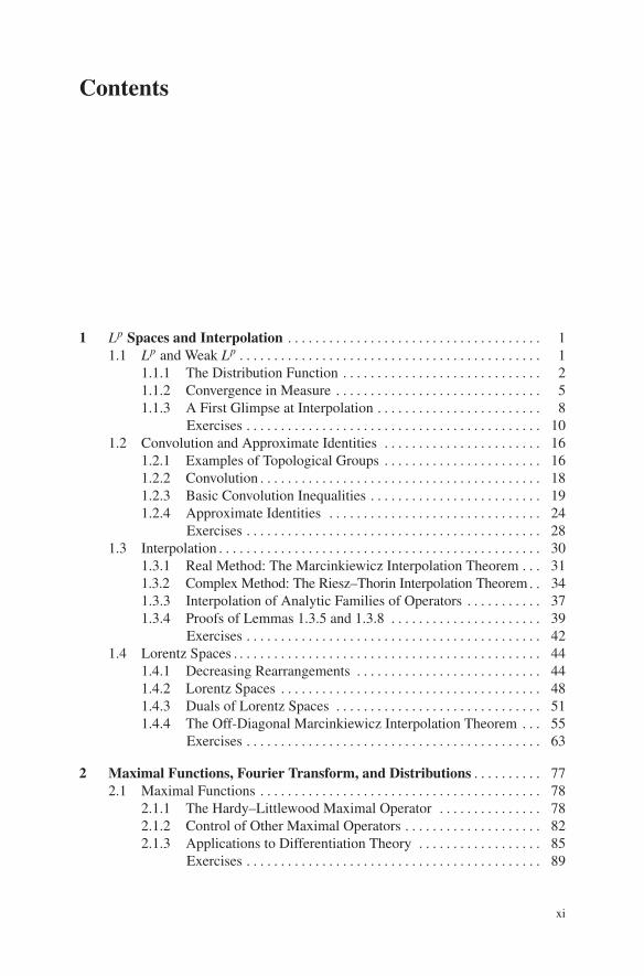
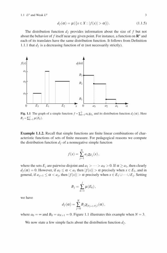
Fig. 1.1 The graph of a simple function f =∑3k=1 akχEk and its distribution function d f (α). Here

B j =∑jk=1 µ(Ek).

Example 1.1.2. Recall that simple functions are finite linear combinations of char-acteristic functions of sets of finite measure. For pedagogical reasons we computethe distribution function d f of a nonnegative simple function

f (x) =N

∑j=1

a jχE j(x) ,

where the sets E j are pairwise disjoint and a1 > · · ·> aN > 0. If α ≥ a1, then clearlyd f (α) = 0. However, if a2 ≤ α < a1 then | f (x)|> α precisely when x ∈ E1, and ingeneral, if a j+1 ≤ α < a j, then | f (x)|> α precisely when x ∈ E1∪·· ·∪E j. Setting

B j =j

∑k=1

µ(Ek) ,

we have

d f (α) =N

∑j=0

B jχ[a j+1,a j)(α) ,

where a0 = ∞ and B0 = aN+1 = 0. Figure 1.1 illustrates this example when N = 3.

We now state a few simple facts about the distribution function d f .

Proposition 1.1.3. Let f and g be measurable functions on (X ,µ). Then for allα,β > 0 we have

(1) |g| ≤ | f | µ-a.e. implies that dg ≤ d f ;

(2) dc f (α) = d f (α/|c|), for all c ∈ C\0;

(3) d f +g(α +β )≤ d f (α)+dg(β );

(4) d f g(αβ )≤ d f (α)+dg(β ).

Proof. The simple proofs are left to the reader.

Knowledge of the distribution function d f provides sufficient information to eval-uate the Lp norm of a function f precisely. We state and prove the following impor-tant description of the Lp norm in terms of the distribution function.

Proposition 1.1.4. For f in Lp(X ,µ), 0 α dµ(x)dα

=∫

X

∫ | f (x)|

0pα

p−1 dα dµ(x)

=∫

X| f (x)|p dµ(x)

=∥∥ f∥∥p

Lp ,

where we used Fubini’s theorem in the second equality. This proves (1.1.6).

Notice that the same argument yields the more general fact that for any increasingcontinuously differentiable function ϕ on [0,∞) with ϕ(0) = 0 we have∫

Xϕ(| f |)dµ =

∫∞

0ϕ′(α)d f (α)dα . (1.1.7)

Definition 1.1.5. For 0 0 : d f (α)≤ Cp

α p for all α > 0

(1.1.8)

= sup

γ d f (γ)1/p : γ > 0

(1.1.9)

is finite. The space weak-L∞(X ,µ) is by definition L∞(X ,µ).

The reader should check that (1.1.9) and (1.1.8) are in fact equal. The weak Lp

spaces are denoted by Lp,∞(X ,µ). Two functions in Lp,∞(X ,µ) are considered equal

if they are equal µ-a.e. The notation Lp,∞(Rn) is reserved for Lp,∞(Rn, | · |). UsingProposition 1.1.3 (2), we can easily show that∥∥k f

∥∥Lp,∞ = |k|

∥∥ f∥∥

Lp,∞ , (1.1.10)

for any complex nonzero constant k. The analogue of (1.1.3) is∥∥ f +g∥∥

Lp,∞ ≤ cp(∥∥ f

∥∥Lp,∞ +

∥∥g∥∥

Lp,∞

), (1.1.11)

where cp = max(2,21/p), a fact that follows from Proposition 1.1.3 (3), taking bothα and β equal to α/2. We also have that∥∥ f

∥∥Lp,∞(X ,µ) = 0⇒ f = 0 µ-a.e. (1.1.12)

In view of (1.1.10), (1.1.11), and (1.1.12), Lp,∞ is a quasinormed linear space for0 < p < ∞.

The weak Lp spaces are larger than the usual Lp spaces. We have the following:

Proposition 1.1.6. For any 0 α

| f (x)|p dµ(x) . (1.1.13)

The integral in (1.1.13) is at most∥∥ f∥∥p

Lp and using (1.1.9) we obtain that∥∥ f∥∥

Lp,∞ ≤∥∥ f∥∥

Lp .

The inclusion Lp ⊆ Lp,∞ is strict. For example, on Rn with the usual Lebesguemeasure, let h(x) = |x|−

np . Obviously, h is not in Lp(Rn) but h is in Lp,∞(Rn) with∥∥h

∥∥Lp,∞(Rn) = vn, where vn is the measure of the unit ball of Rn.

It is not immediate from their definition that the weak Lp spaces are completewith respect to the quasinorm

∥∥ ·∥∥Lp,∞ . The completeness of these spaces is provedin Theorem 1.4.11, but it is also a consequence of Theorem 1.1.13, proved in thissection.

1.1.2 Convergence in Measure

Next we discuss some convergence notions. The following notion is important inprobability theory.

Definition 1.1.7. Let f , fn, n = 1,2, . . . , be measurable functions on the measurespace (X ,µ). The sequence fn is said to converge in measure to f if for all ε > 0there exists an n0 ∈ Z+ such that

n > n0 =⇒ µ(x ∈ X : | fn(x)− f (x)|> ε) < ε . (1.1.14)

Remark 1.1.8. The preceding definition is equivalent to the following statement:

For all ε > 0 limn→∞

µ(x ∈ X : | fn(x)− f (x)|> ε) = 0 . (1.1.15)

Clearly (1.1.15) implies (1.1.14). To see the converse given ε > 0, pick 0 < δ < ε

and apply (1.1.14) for this δ . There exists an n0 ∈ Z+ such that

µ(x ∈ X : | fn(x)− f (x)|> δ) < δ

holds for n > n0. Since

µ(x ∈ X : | fn(x)− f (x)|> ε)≤ µ(x ∈ X : | fn(x)− f (x)|> δ) ,

we conclude thatµ(x ∈ X : | fn(x)− f (x)|> ε) < δ

for all n > n0. Let n→ ∞ to deduce that

limsupn→∞

µ(x ∈ X : | fn(x)− f (x)|> ε)≤ δ . (1.1.16)

Since (1.1.16) holds for all 0 < δ < ε , (1.1.15) follows by letting δ → 0.Convergence in measure is a weaker notion than convergence in either Lp or Lp,∞,

0 < p≤ ∞, as the following proposition indicates:

Proposition 1.1.9. Let 0 < p≤ ∞ and fn, f be in Lp,∞(X ,µ).

(1) If fn, f are in Lp and fn → f in Lp, then fn → f in Lp,∞.(2) If fn → f in Lp,∞, then fn converges to f in measure.

Proof. Fix 0 0 we have

µ(x ∈ X : | fn(x)− f (x)|> ε)≤ 1ε p

∫X| fn− f |p dµ .

This shows that convergence in Lp implies convergence in weak Lp. The case p = ∞

is tautological.Given ε > 0 find an n0 such that for n > n0, we have∥∥ fn− f

∥∥Lp,∞ = sup

α>0αµ(x ∈ X : | fn(x)− f (x)|> α)

1p < ε

1p +1 .

Taking α = ε , we conclude that convergence in Lp,∞ implies convergence in mea-sure.

Example 1.1.10. Fix 0 < p < ∞. On [0,1] define the functions

fk, j = k1/pχ( j−1

k , jk ), k ≥ 1, 1≤ j ≤ k.

Consider the sequence f1,1, f2,1, f2,2, f3,1, f3,2, f3,3, . . .. Observe that

|x : fk, j(x) > 0|= 1/k .

Therefore, fk, j converges to 0 in measure. Likewise, observe that

∥∥ fk, j∥∥

Lp,∞ = supα>0

α|x : fk, j(x) > α|1/p ≥ supk≥1

(k−1/k)1/p

k1/p = 1 ,

which implies that fk, j does not converge to 0 in Lp,∞.

It turns out that every sequence convergent in Lp(X ,µ) or in Lp,∞(X ,µ) has asubsequence that converges a.e. to the same limit.

Theorem 1.1.11. Let fn and f be complex-valued measurable functions on a mea-sure space (X ,µ) and suppose that fn converges to f in measure. Then some subse-quence of fn converges to f µ-a.e.

Proof. For all k = 1,2, . . . choose inductively nk such that

µ(x ∈ X : | fnk(x)− f (x)|> 2−k) < 2−k (1.1.17)

and such that n1 < n2 < · · ·< nk < · · · . Define the sets

Ak = x ∈ X : | fnk(x)− f (x)|> 2−k .

Equation (1.1.17) implies that

µ

( ∞⋃k=m

Ak

)≤

∞

∑k=m

µ(Ak)≤∞

∑k=m

2−k = 21−m (1.1.18)

for all m = 1,2,3, . . . . It follows from (1.1.18) that

µ

( ∞⋃k=1

Ak

)≤ 1 < ∞ . (1.1.19)

Using (1.1.18) and (1.1.19), we conclude that the sequence of the measures of thesets

⋃∞k=m Ak∞

m=1 converges as m→ ∞ to

µ

( ∞⋂m=1

∞⋃k=m

Ak

)= 0 . (1.1.20)

To finish the proof, observe that the null set in (1.1.20) contains the set of all x ∈ Xfor which fnk(x) does not converge to f (x).

In many situations we are given a sequence of functions and we would like toextract a convergent subsequence. One way to achieve this is via the next theorem,which is a useful variant of Theorem 1.1.11. We first give a relevant definition.

Definition 1.1.12. We say that a sequence of measurable functions fn on the mea-sure space (X ,µ) is Cauchy in measure if for every ε > 0, there exists an n0 ∈ Z+

such that for n,m > n0 we have

µ(x ∈ X : | fm(x)− fn(x)|> ε) < ε.

Theorem 1.1.13. Let (X ,µ) be a measure space and let fn be a complex-valuedsequence on X that is Cauchy in measure. Then some subsequence of fn convergesµ-a.e.

Proof. The proof is very similar to that of Theorem 1.1.11. For all k = 1,2, . . .choose nk inductively such that

µ(x ∈ X : | fnk(x)− fnk+1(x)|> 2−k) < 2−k (1.1.21)

and such that n1 < n2 < · · ·< nk < nk+1 < · · · . Define

Ak = x ∈ X : | fnk(x)− fnk+1(x)|> 2−k .

As shown in the proof of Theorem 1.1.11, (1.1.21) implies that

µ

( ∞⋂m=1

∞⋃k=m

Ak

)= 0 . (1.1.22)

For x /∈⋃

∞k=m Ak and i≥ j ≥ j0 ≥ m (and j0 large enough) we have

| fni(x)− fn j(x)| ≤i−1

∑l= j| fnl (x)− fnl+1(x)| ≤

i−1

∑l= j

2−l ≤ 21− j ≤ 21− j0 .

This implies that the sequence fni(x)i is Cauchy for every x in the set (⋃

∞k=m Ak)c

and therefore converges for all such x. We define a function

f (x) =

limj→∞

fn j(x) when x /∈⋂

∞m=1

⋃∞k=m Ak ,

0 when x ∈⋂

∞m=1

⋃∞k=m Ak .

Then fn j → f almost everywhere.

1.1.3 A First Glimpse at Interpolation

It is a useful fact that if a function f is in Lp(X ,µ) and in Lq(X ,µ), then it also liesin Lr(X ,µ) for all p < r < q. The usefulness of the spaces Lp,∞ can be seen fromthe following sharpening of this statement:

Proposition 1.1.14. Let 0 < p < q ≤ ∞ and let f in Lp,∞(X ,µ)∩Lq,∞(X ,µ). Thenf is in Lr(X ,µ) for all p < r < q and

∥∥ f∥∥

Lr ≤(

rr− p

+r

q− r

)1r ∥∥ f∥∥ 1

r −1q

1p−

1q

Lp,∞

∥∥ f∥∥ 1

p−1r

1p−

1q

Lq,∞ , (1.1.23)

with the suitable interpretation when q = ∞.

Proof. Let us take first q < ∞. We know that

d f (α)≤min(∥∥ f

∥∥pLp,∞

α p ,

∥∥ f∥∥q

Lq,∞

αq

). (1.1.24)

Set

B =(∥∥ f

∥∥qLq,∞∥∥ f∥∥p

Lp,∞

) 1q−p

. (1.1.25)

We now estimate the Lr norm of f . By (1.1.24), (1.1.25), and Proposition 1.1.4 wehave ∥∥ f

∥∥rLr(X ,µ) = r

∫∞

0α

r−1d f (α)dα

≤ r∫

∞

0α

r−1 min(∥∥ f

∥∥pLp,∞

α p ,

∥∥ f∥∥q

Lq,∞

αq

)dα

= r∫ B

0α

r−1−p∥∥ f∥∥p

Lp,∞ dα + r∫

∞

Bα

r−1−q∥∥ f∥∥q

Lq,∞ dα

=r

r− p

∥∥ f∥∥p

Lp,∞Br−p +r

q− r

∥∥ f∥∥q

Lq,∞Br−q

=(

rr− p

+r

q− r

)(∥∥ f∥∥p

Lp,∞

) q−rq−p(∥∥ f

∥∥qLq,∞

) r−pq−p .

(1.1.26)

Observe that the integrals converge, since r− p > 0 and r−q < 0.The case q = ∞ is easier. Since d f (α) = 0 for α >

∥∥ f∥∥

L∞ we need to use onlythe inequality d f (α)≤ α−p

∥∥ f∥∥p

Lp,∞ for α ≤∥∥ f∥∥

L∞ in estimating the first integral in(1.1.26). We obtain ∥∥ f

∥∥rLr ≤

rr− p

∥∥ f∥∥p

Lp,∞

∥∥ f∥∥r−p

L∞ ,

which is nothing other than (1.1.23) when q = ∞. This completes the proof.

Note that (1.1.23) holds with constant 1 if Lp,∞ and Lq,∞ are replaced by Lp andLq, respectively. It is often convenient to work with functions that are only locallyin some Lp space. This leads to the following definition.

Definition 1.1.15. For 0 < p < ∞, the space Lploc(R

n, | · |) or simply Lploc(R

n) is theset of all Lebesgue-measurable functions f on Rn that satisfy∫

K| f (x)|p dx < ∞ (1.1.27)

for any compact subset K of Rn. Functions that satisfy (1.1.27) with p = 1 are calledlocally integrable functions on Rn.

The union of all Lp(Rn) spaces for 1 ≤ p ≤ ∞ is contained in L1loc(R

n). Moregenerally, for 0 < p < q < ∞ we have the following:

Lq(Rn)⊆ Lqloc(R

n)⊆ Lploc(R

n) .

Functions in Lp(Rn) for 0 < p < 1 may not be locally integrable. For example, takef (x) = |x|−n−α χ|x|≤1, which is in Lp(Rn) when p < n/(n + α), and observe that fis not integrable over any open set in Rn containing the origin.

Exercises

1.1.1. Suppose f and fn are measurable functions on (X ,µ). Prove that(a) d f is right continuous on [0,∞).(b) If | f | ≤ liminfn→∞ | fn| µ-a.e., then d f ≤ liminfn→∞ d fn .(c) If | fn| ↑ | f |, then d fn ↑ d f .[Hint: Part (a): Let tn be a decreasing sequence of positive numbers that tends to

zero. Show that d f (α0 + tn) ↑ d f (α0) using a convergence theorem. Part (b): LetE = x ∈ X : | f (x)|> α and En = x ∈ X : | fn(x)|> α. Use that µ

(⋂∞n=m En

)≤

liminfn→∞

µ(En) and E ⊆⋃

∞m=1

⋂∞n=m En µ-a.e.

]1.1.2. (Holder’s inequality ) Let 0 < p, p1, . . . , pk ≤∞, where k≥ 2, and let f j be inLp j = Lp j(X ,µ). Assume that

1p

=1p1

+ · · ·+ 1pk

.

(a) Show that the product f1 · · · fk is in Lp and that∥∥ f1 · · · fk∥∥

Lp ≤∥∥ f1∥∥

Lp1 · · ·∥∥ fk∥∥

Lpk .

(b) When no p j is infinite, show that if equality holds in part (a), then it must be thecase that c1| f1|p1 = · · ·= ck| fk|pk a.e. for some c j ≥ 0.(c) Let 0 < q < 1. For r < 0 and g > 0 almost everywhere, let

∥∥g∥∥

Lr =∥∥g−1

∥∥−1L|r| .

Show that for f ≥ 0, g > 0 a.e. we have∥∥ f g∥∥

L1 ≥∥∥ f∥∥

Lq

∥∥g∥∥

Lq′ .

1.1.3. Let (X ,µ) be a measure space.(a) If f is in Lp0(X ,µ) for some p0 < ∞, prove that

limp→∞

∥∥ f∥∥

Lp =∥∥ f∥∥

L∞ .

(b) (Jensen’s inequality ) Suppose that µ(X) = 1. Show that

∥∥ f∥∥

Lp ≥ exp(∫

Xlog | f (x)|dµ(x)

)for all 0 0, then

limp→0

∥∥ f∥∥

Lp = exp(∫

Xlog | f (x)|dµ(x)

)with the interpretation e−∞ = 0.[Hint: Part (a): Given 0 < ε < ‖ f‖L∞ , find a measurable set E ⊆ X of positive mea-

sure such that | f (x)| ≥ ‖ f‖L∞ − ε for all x ∈ E. Then ‖ f‖Lp ≥ (‖ f‖L∞ − ε)µ(E)1/p

and thus liminfp→∞ ‖ f‖Lp ≥ ‖ f‖L∞ −ε . Part (b) is a direct consequence of Jensen’sinequality

∫X log |h|dµ ≤ log

(∫X |h|dµ

). Part (c): Fix a sequence 0 < pn < p0 such

that pn ↓ 0 and define

hn(x) =1p0

(| f (x)|p0 −1)− 1pn

(| f (x)|pn −1).

Use that 1p (t p−1) ↓ log t as p ↓ 0 for all t > 0. The Lebesgue monotone convergence

theorem yields∫

X hn dµ ↑∫

X hdµ , hence∫

X1pn

(| f |pn −1)dµ ↓∫

X log | f |dµ , wherethe latter could be −∞. Use

exp(∫

Xlog | f |dµ

)≤(∫

X| f |pn dµ

) 1pn≤ exp

(∫X

1pn

(| f |pn −1)dµ

)to complete the proof.

]1.1.4. Let a j be a sequence of positive reals. Show that(a)(

∑∞j=1 a j

)θ ≤ ∑∞j=1 aθ

j , for any 0≤ θ ≤ 1.

(b) ∑∞j=1 aθ

j ≤(

∑∞j=1 a j

)θ, for any 1≤ θ < ∞.

(c)(

∑Nj=1 a j

)θ ≤ Nθ−1∑

Nj=1 aθ

j , when 1≤ θ < ∞.

(d) ∑Nj=1 aθ

j ≤ N1−θ(

∑Nj=1 a j

)θ , when 0≤ θ ≤ 1.

1.1.5. Let f jNj=1 be a sequence of Lp(X ,µ) functions.

(a) (Minkowski’s inequality ) For 1≤ p≤ ∞ show that

∥∥ N

∑j=1

f j∥∥

Lp ≤N

∑j=1

∥∥ f j∥∥

Lp .

(b) (Minkowski’s inequality ) For 0 < p < 1 and f j ≥ 0 prove that

N

∑j=1

∥∥ f j∥∥

Lp ≤∥∥ N

∑j=1

f j∥∥

Lp .

(c) For 0 < p < 1 show that

∥∥ N

∑j=1

f j∥∥

Lp ≤ N1−p

pN

∑j=1

∥∥ f j∥∥

Lp .

(d) The constant N1−p

p in part (c) is best possible.[Hint: Part (c): Use Exercise 1.1.4(c). Part (d): Take f jN

j=1 to be characteristicfunctions of disjoint sets with the same measure.

]1.1.6. (Minkowski’s integral inequality ) Let 1 ≤ p < ∞. Let F be a measurablefunction on the product space (X ,µ)× (T,ν), where µ,ν are σ -finite. Show that[∫

T

(∫X|F(x, t)|dµ(x)

)p

dν(t)] 1

p

≤∫

X

[∫T

∣∣F(x, t)∣∣p dν(t)

] 1p

dµ(x) .

Moreover, prove that when 0 < p < 1, then the preceding inequality is reversed.

1.1.7. Let f1, . . . , fN be in Lp,∞(X ,µ).(a) Prove that for 1≤ p < ∞ we have

∥∥ N

∑j=1

f j∥∥

Lp,∞ ≤ NN

∑j=1

∥∥ f j∥∥

Lp,∞ .

(b) Show that for 0 α) ≤ ∑

Nj=1 µ(| f j| > α/N) and Exercise

1.1.4(a) and (c).]

1.1.8. Let 0 < p < ∞. Prove that Lp(X ,µ) is a complete quasinormed space. Thismeans that every quasinorm Cauchy sequence is quasinorm convergent.[Hint: Let fn be a Cauchy sequence in Lp. Pass to a subsequence nii such that‖ fni+1 − fni‖Lp ≤ 2−i. Then the series f = fn1 +∑

∞i=1( fni+1 − fni) converges in Lp.

]1.1.9. Let (X ,µ) be a measure space with µ(X) < ∞. Suppose that a sequence ofmeasurable functions fn on X converges to f µ-a.e. Prove that fn converges to f inmeasure.[Hint: For ε > 0,

x ∈ X : fn(x)→ f (x)j

∞⋃m=1

∞⋂n=m

x ∈ X : | fn(x)− f (x)|< ε.]

1.1.10. Given a measurable function f on (X ,µ) and γ > 0, define fγ = f χ| f |>γ andf γ = f − fγ = f χ| f |≤γ .(a) Prove that

d fγ (α) =

d f (α) when α > γ,

d f (γ) when α ≤ γ,

d f γ (α) =

0 when α ≥ γ,

d f (α)−d f (γ) when α < γ.

(b) If f ∈ Lp(X ,µ) then∥∥ fγ

∥∥pLp = p

∫∞

γ

αp−1d f (α)dα + γ

pd f (γ),∥∥ f γ∥∥p

Lp = p∫

γ

0α

p−1d f (α)dα− γpd f (γ),∫

γ<| f |≤δ

| f |p dµ = p∫

δ

γ

d f (α)α p−1 dα−δpd f (δ )+ γ

pd f (γ).

(c) If f is in Lp,∞(X ,µ) prove that f γ is in Lq(X ,µ) for any q > p and fγ is inLq(X ,µ) for any q < p. Thus Lp,∞ ⊆ Lp0 +Lp1 when 0 < p0 < p < p1 ≤ ∞.

1.1.11. Let (X ,µ) be a measure space and let E be a subset of X with µ(E) < ∞.Assume that f is in Lp,∞(X ,µ) for some 0 < p < ∞.(a) Show that for 0 < q α

)≤min

(µ(E),α−p

∥∥ f∥∥p

Lp,∞

).]

1.1.12. (Normability of weak Lp for p > 1 ) Let (X ,µ) be a measure space and let0 < p < ∞. Pick 0 < r < p and define

f

Lp,∞ = sup0<µ(E)<∞

µ(E)−1r + 1

p

(∫E| f |rdµ

) 1r

,

where the supremum is taken over all measurable subsets E of X of finite measure.(a) Use Exercise 1.1.11 with q = r to conclude that

f

Lp,∞ ≤(

pp− r

) 1r ∥∥ f∥∥

Lp,∞

for all f in Lp,∞(X ,µ).(b) Take E = | f |> α to deduce that

∥∥ f∥∥

Lp,∞ ≤ f

Lp,∞ for all f in Lp,∞(X ,µ).

(c) Show that Lp,∞(X ,µ) is metrizable for all 0 1(by picking r = 1).(d) Use the characterization of the weak Lp quasinorm obtained in parts (a) and (b)to prove Fatou’s theorem for this space: For all measurable functions gn on X wehave ∥∥ liminf

n→∞|gn|∥∥

Lp,∞ ≤Cp liminfn→∞

∥∥gn∥∥

Lp,∞

for some constant Cp that depends only on p ∈ (0,∞).

1.1.13. Consider the N! functions on the line

fσ =N

∑j=1

Nσ( j)

χ[ j−1N , j

N ) ,

where σ is a permutation of the set 1,2, . . . ,N.(a) Show that each fσ satisfies

∥∥ fσ

∥∥L1,∞ = 1.

(b) Show that∥∥∑σ∈SN fσ

∥∥L1,∞ = N!

(1+ 1

2 + · · ·+ 1N

).

(c) Conclude that the space L1,∞(R) is not normable.(d) Use a similar argument to prove that L1,∞(Rn) is not normable by consideringthe functions

fσ (x1, . . . ,xn) =N

∑j1=1

· · ·N

∑jn=1

Nn

σ(τ( j1, . . . , jn))χ

[ j1−1N ,

j1N )

(x1) · · ·χ[ jn−1N , jn

N )(xn) ,

where σ is a permutation of the set 1,2, . . . ,Nn and τ is a fixed injective mapfrom the set of all n-tuples of integers with coordinates 1 ≤ j ≤ N onto the set1,2, . . . ,Nn. One may take

τ( j1, . . . , jn) = j1 +N( j2−1)+N2( j3−1)+ · · ·+Nn−1( jn−1),

for instance.

1.1.14. Let 0 < p < 1, 0 < s < ∞ and let (X ,µ) be a measure space.(a) Let f be a measurable function on X . Show that∫

| f |≤s| f |dµ ≤ s1−p

1− p

∥∥ f∥∥p

Lp,∞ .

(b) Let f j, 1≤ j ≤ m, be measurable functions on X . Show that∥∥∥ max1≤ j≤m

| f j|∥∥∥p

Lp,∞≤

m

∑j=1

∥∥ f j∥∥p

Lp,∞ .

(c) Conclude that

1.1 Lp and Weak Lp 15∥∥ f1 + · · ·+ fm∥∥p

Lp,∞ ≤2− p1− p

m

∑j=1

∥∥ f j∥∥p

Lp,∞ .

The latter estimate is referred to as the p-normability of weak Lp for p < 1.[Hint: Part (c): First obtain the estimate

d f1+···+ fm(α) ≤ µ(| f1+· · ·+ fm|>α,max | f j|≤α)+dmax | f j |(α)

for all α > 0.]

1.1.15. (Holder’s inequality for weak spaces ) Let f j be in Lp j ,∞ of a measure spaceX where 0 < p j < ∞ and 1≤ j ≤ k. Let

1p

=1p1

+ · · ·+ 1pk

.

Prove that ∥∥ f1 · · · fk∥∥

Lp,∞ ≤ p−1p

k

∏j=1

p1p jj

k

∏j=1

∥∥ f j∥∥

Lp j ,∞ .

[Hint: Take ‖ f j‖Lp j ,∞ = 1 for all j. Control d f1··· fk(α) by

µ(| f1|>α/s1)+ · · ·+ µ(| fk−1|>sk−2/sk−1)+ µ(| fk|>sk−1)≤ (s1/α)p1 +(s2/s1)p2 + · · ·+(sk−1/sk−2)pk−1 +(1/sk−1)pk .

Set x1 = s1/α , x2 = s2/s1, . . . ,xk = 1/sk−1. Minimize xp11 + · · ·+ xpk

k subject to theconstraint x1 · · ·xk = 1/α .

]1.1.16. Let 0 < p0 < p < p1 ≤ ∞ and let 1

p = 1−θ

p0+ θ

p1for some θ ∈ [0,1]. Prove

the following: ∥∥ f∥∥

Lp ≤∥∥ f∥∥1−θ

Lp0

∥∥ f∥∥θ

Lp1 ,∥∥ f∥∥

Lp,∞ ≤∥∥ f∥∥1−θ

Lp0,∞

∥∥ f∥∥θ

Lp1,∞ .

1.1.17. (Loomis and Whitney [178] ) Follow the steps below to prove the isoperi-metric inequality. For n ≥ 2 and 1 ≤ j ≤ n define the projection maps π j : Rn →Rn−1 by setting for x = (x1, . . . ,xn),

π j(x) = (x1, . . . ,x j−1,x j+1, . . . ,xn) ,

with the obvious interpretations when j = 1 or j = n.(a) For maps f j : Rn−1 → C prove that

Λ( f1, . . . , fn) =∫

Rn

n

∏j=1

∣∣ f j π j∣∣dx ≤

n

∏j=1

∥∥ f j∥∥

Ln−1(Rn−1) .


(b) Let Ω be a compact set with a rectifiable boundary in Rn where n ≥ 2. Showthat there is a constant cn independent of Ω such that

|Ω | ≤ cn|∂Ω |n

n−1 ,

where the expression |∂Ω | denotes the (n−1)-dimensional surface measure of theboundary of Ω .[Hint: Part (a): Use induction starting with n = 2. Then write

Λ( f1, . . . , fn) ≤∫

Rn−1P(x1, . . . ,xn−1)| fn(πn(x))|dx1 · · ·dxn−1

≤∥∥P∥∥

Ln−1n−2 (Rn−1)

∥∥ fn πn∥∥

Ln−1(Rn−1) ,

where P(x1, . . . ,xn−1) =∫

R | f1(π1(x)) · · · fn−1(πn−1(x))|dxn, and apply the induc-tion hypothesis to the n−1 functions[∫

Rf j(π j(x))n−1 dxn

] 1n−2

,

for j = 1, . . . ,n−1, to obtain the required conclusion. Part (b): Specialize part (a) tothe case f j = χπ j [Ω ] to obtain

|Ω | ≤ |π1[Ω ]|1

n−1 · · · |πn[Ω ]|1

n−1

and then use that |π j[Ω ]| ≤ 12 |∂Ω |.

]

1.2 Convolution and Approximate Identities

The notion of convolution can be defined on measure spaces endowed with a groupstructure. It turns out that the most natural environment to define convolution is thecontext of topological groups. Although the focus of this book is harmonic analysison Euclidean spaces, we develop the notion of convolution on general groups. Thisallows us to study this concept on Rn, Zn, and Tn, in a unified way. Moreover,since the basic properties of convolutions and approximate identities do not requirecommutativity of the group operation, we may assume that the underlying groupsare not necessarily abelian. Thus, the results in this section can be also applied tononabelian structures such as the Heisenberg group.

1.2.1 Examples of Topological Groups

A topological group G is a Hausdorff topological space that is also a group with law

Editorial Board S. Axler K.A. Ribet · x Acknowledgments Roman Shvidkoy, Elias Stein, Atanas...

Documents

Transcript of Editorial Board S. Axler K.A. Ribet · x Acknowledgments Roman Shvidkoy, Elias Stein, Atanas...