Editorial Board - UPT · Editorial Board • Prof. Dr. Eng ... downlink DTX on the traffic channel...
35
Editorial Board • Prof. Dr. Eng. Ioan NAFORNITA, Editor-in-chief • Prof. Dr. Eng. Virgil TIPONUT • Prof. Dr. Eng. Alexandru ISAR • Prof. Dr. Eng. Dorina ISAR • Prof. Dr. Eng. Traian JURCA • Prof. Dr. Eng. Aldo DE SABATA • Prof. Dr. Eng. Florin ALEXA • Prof. Dr. Eng. Radu VASIU • Lecturer Dr. Eng. Maria KOVACI, Scientific Secretary • Associate Prof. Dr. Eng. Corina NAFORNITA, Scientific Secretary Scientific Board • Prof. Dr. Eng. Monica BORDA, Technical University of Cluj-Napoca, Romania • Prof. Dr. Eng. Aldo DE SABATA, Politehnica University of Timisoara, Romania • Prof. Dr. Eng. Karen EGUIAZARIAN, Tampere University of Technology, Institute of Signal Processing, Finland • Prof. Dr. Eng. Liviu GORAS, Technical University Gheorghe Asachi, Iasi, Romania • Prof. Dr. Eng. Alexandru ISAR, Politehnica University of Timisoara, Romania • Prof. Dr. Eng. Michel JEZEQUEL, TELECOM Bretagne, Brest, France • Prof. Dr. Eng. Traian JURCA, Politehnica University of Timisoara, Romania • Prof. Dr. Eng. Ioan NAFORNITA, Politehnica University of Timisoara, Romania • Prof. Dr. Eng. Mohamed NAJIM, ENSEIRB Bordeaux, France • Prof. Dr. Eng. Emil PETRIU, SITE, University of Ottawa, Canada • Prof. Dr. Eng. Andre QUINQUIS, Ministère de la Défense, Paris, France
Transcript of Editorial Board - UPT · Editorial Board • Prof. Dr. Eng ... downlink DTX on the traffic channel...

Editorial Board
• Prof. Dr. Eng. Ioan NAFORNITA, Editor-in-chief
• Prof. Dr. Eng. Virgil TIPONUT • Prof. Dr. Eng. Alexandru ISAR • Prof. Dr. Eng. Dorina ISAR • Prof. Dr. Eng. Traian JURCA • Prof. Dr. Eng. Aldo DE SABATA • Prof. Dr. Eng. Florin ALEXA • Prof. Dr. Eng. Radu VASIU
• Lecturer Dr. Eng. Maria KOVACI, Scientific Secretary • Associate Prof. Dr. Eng. Corina NAFORNITA, Scientific
Secretary
Scientific Board
• Prof. Dr. Eng. Monica BORDA, Technical University of Cluj-Napoca, Romania
• Prof. Dr. Eng. Aldo DE SABATA, Politehnica University of Timisoara, Romania
• Prof. Dr. Eng. Karen EGUIAZARIAN, Tampere University of Technology, Institute of Signal Processing, Finland
• Prof. Dr. Eng. Liviu GORAS, Technical University Gheorghe Asachi, Iasi, Romania
• Prof. Dr. Eng. Alexandru ISAR, Politehnica University of Timisoara, Romania
• Prof. Dr. Eng. Michel JEZEQUEL, TELECOM Bretagne, Brest, France
• Prof. Dr. Eng. Traian JURCA, Politehnica University of Timisoara, Romania
• Prof. Dr. Eng. Ioan NAFORNITA, Politehnica University of Timisoara, Romania
• Prof. Dr. Eng. Mohamed NAJIM, ENSEIRB Bordeaux, France
• Prof. Dr. Eng. Emil PETRIU, SITE, University of Ottawa, Canada
• Prof. Dr. Eng. Andre QUINQUIS, Ministère de la Défense, Paris, France
• Prof. Dr. Eng. Maria Victoria RODELLAR BIARGE, Polytechnic University of Madrid, Spain
• Prof. Dr. Eng. Alexandru SERBANESCU, Technical Military Academy, Bucharest, Romania
• Prof. Dr. Eng. Virgil TIPONUT, Politehnica University of Timisoara, Romania
• Prof. Dr. Eng. Radu VASIU, Politehnica University of Timisoara, Romania
Advisory Board
• Prof. Dr. Eng. Ioan NAFORNITA, Politehnica University of Timisoara, Romania
• Prof. Dr. Eng. Alexandru ISAR, Politehnica University of Timisoara, Romania
• Prof. Dr. Eng. Mihaela LASCU, Politehnica University of Timisoara, Romania
• Prof. Dr. Eng. Florin ALEXA, Politehnica University of Timisoara, Romania
• Prof. Dr. Eng. Vasile GUI, Politehnica University of Timisoara, Romania
• Associate Prof. Dr. Eng. Eugen MARZA, Politehnica University of Timisoara, Romania
• Associate Prof. Dr. Eng. Dan ANDREICIUC, Politehnica University of Timisoara, Romania
• As. Dr. Ing. Andy VESA, Politehnica University of Timisoara, Romania

Buletinul Ştiinţific al Universităţii Politehnica Timişoara
TRANSACTIONS on ELECTRONICS and COMMUNICATIONS
Volume 59(73), Issue 1, 2014
CONTENTS
Cătălina-Marina Crina:
"Study on Coexistence between Long Term Evolution and Global System for Mobile
Communication"........................................................................................................................ 3
Razvan-Marius Popa:
"RAN Dimensioning for Wireless Networks"................................................................ 8
Ioana-Elena Puşcaş:
"Carrier Aggregation in LTE-Advanced"................................................................... 13
Victor Serban, Dan Andreiciuc, Aurel Filip:
"Telemetric Applications for the Automotive Industry using IQRF devices".............. 17
Cătălin Tudoran, Dan Andreiciuc, Aurel Filip:
"Multifunctional Siren for Emergency Services"........................................................ 21
Lupou Cristian Marius:
"Modeling in Matlab/Simulink the control of the vehicle’s air conditioner
compressor"............................................................................................................................. 26
Instructions for authors at the Scientific Bulletin of the Politehnica University of Timisoara -
Transactions on Electronics and Communications ................................................................ 32
1

2

Buletinul Ştiinţific al Universităţii Politehnica Timişoara
TRANSACTIONS on ELECTRONICS and COMMUNICATIONS
Volume 59(73), Issue 1, 2014
Study on Coexistence between Long Term Evolution and
Global System for Mobile Communication
Cătălina-Marina Crina 1
1 Faculty of Electronics and Telecommunications, Communications Dept.
Bd. V. Parvan 2, 300223 Timisoara, Romania, e-mail [email protected]
Abstract — The massive development in mobile and
personal communications and the emergence of a
diversity of radio applications and services has led to an
explosion in the number of base station sites and mobile
stations and it is emphasizing the necessity for
improvements in the way that network operators co-
exist. Sustaining future growth is strongly dependent
upon the efficiency with which the radio spectrum is
used.
The main purpose of this paper is to evaluate the
possibility of co-existence between the GSM and LTE
systems using a software tool based upon Monte Carlo
technique, so called the Spectrum Engineering
Advanced Monte Carlo Analysis Tool (SEAMCAT),
identify the potential problems that might occur and
eventually draw conclusions and emphasize proper
solutions for the occurred problems.
Keywords — co-existence, interference, GSM, LTE
Monte Carlo, SEAMCAT
I. INTRODUCTION
Co-location or co-existence in near vicinity of Base
Stations may cause interference resulting in
performance degradation. In order to minimize this
performance degradation to an acceptable defined
level, certain decoupling requirements between the
systems have to be met. Actual decoupling
requirements can be estimated using comprehensive
interference analysis techniques.
The most critical co-existence situations occur when
the Down Link (DL) of any system (the interfering
one) is close to the Up Link (UL) of the concerned
victim system. In that case an interfering Base Station
(BS) is constantly disturbing a victim system BS
probably with high gain antennas on both sides.
Mobile Stations (MSs) may also be close to each
other and cause interference but this happens only
occasionally. BS and MS may also interferer each
other in special situations, caused by the near far
problems.
The assessment methodology for mobile inter-system
compatibility for site co-existence, site co-location
and sharing consists in the three main steps:
- Listing the possible incompatibility problems;
- Interference analysis;
- Required decoupling implementation solution.
The scope of this first step is to get a list of possible
reciprocal impact of the given systems in terms of
interferences. It is desirable (but often impossible) to
rank the interference sources upon their impact’s
severity.
The goal of the second step is to obtain the necessary
decoupling value between systems or the probability
of interference, depending on the calculation method
used.
There are two methods used for interference
assessment:
- deterministic calculation, which provides decoupling
requirement values which must be implemented
between the two systems;
- statistical method based on Monte Carlo simulations,
which provides the probability of interference
between the two systems.
The last step it consists of considering some case
specific solutions:
- improvement of cell planning such as: shrinking the
interfering cell, for example by lowering its output
power or tilting the antennas of its base station (if
feasible),
- increasing the stopband attenuation of the interfering
system’s transmit filter in the receive band of the
victim system,
- increasing the stopband attenuation of the interfering
system’s transmit filter in the transmit band of the co-
located system. This minimizes coupling between the
transmitters and the generated IM products in the
transmitters.
- increasing the receive filter’s stopband attenuation
for the interfering transmit frequencies, so that the
levels of these transmit signals are lowered below the
critical value,
- increasing decoupling between the two systems,
either the air decoupling or the decoupling provided
by diplexer. This also minimizes coupling between
the transmitters.
- other system specific measures such as activating
downlink DTX on the traffic channel or activating
downlink power control on traffic channels in the case
of the GSM system will be lower.
3

II. SPECTRUM ENGINEERING ADVANCED
MONTE CARLO ANALYSIS TOOL (SEAMCAT)
Using Monte Carlo method, in many applications the
physical process is directly simulated, hence there is
no need to write the differential equations describing
the behavior of the system, unlike the classical
analysis methods which use differential equations.The
only requirement is that the physical or mathematical
system to be described using probability and density
functions. The result is extracted by averaging a
number of simulations for a certain number of cases
[2].
The SEAMCAT simulator models a victim receiver
which operates in a medium with multiple sources of
interference. The interference sources may belong to
the same system as the victim receiver, or to another
system. The interference sources are randomly
distributed around the victim in a manner chosen by
the user. Usually a uniform distribution is chosen.
Only a specific number of sources of interference are
active at a time. In the figure 1, there is presented a
simulation scenario with a victim receiver and its
sources of interference.
The effect of each source of interference is accounted.
Some interference mechanisms are also included:
unwanted emissions, receiver blocking,
intermodulation products, co-channel and adjacent
channel interference [2]. A condition of interference occurrence is that the
victim receiver to have a carrier to interference ratio
(C/I) smaller than the minimum accepted value for a
correct decoding. In order to compute the carrier to
interference ratio of the victim, it is necessary to
establish both the desired received signal strength
(dRSS) and interfering received signal strength
(iRSS), [2].
On the left side of the diagram, the situation when no
interference occurs is presented, and on the right side
the opposite is presented. In the latter case, the
additional interference inside the wanted channel
Fig 1 A typical interference scenario for a Monte Carlo simulation,
[2].
Fig 2 Diagram of the received signals and C/I ratio [2].
band, will increase the noise level, and consequently
the C/I ratio of the victim system will decrease. The
new C/I ratio is defined by the difference in dB
between desired signal strength and the increased
noise level. This ratio has to be greater than the
minimum accepted in order to obtain a correct
decoding, [2].
The SEAMCAT tool verifies this condition and it
registers, for each case, whether interference occurred.
The Monte Carlo method considers independent
situations in time (or space). For each situation, a
scenario is built using a certain number of different
variables: the interfering sources position in relation
to the victim, the desired signal strength, the channels
used by the victim receiver and the interferer, and so
on. If a sufficient number of simulations are taken into
account, the probability of interference can be
computed with a higher precision, [2].
III. STUDY CASE – INTERFERENCE
ASSESSMENT BETWEEN LEGACY GSM AND
4G LTE IN 900 MHZ BAND
This study focuses on the main interference problems
which may appear with the introduction of new
generation LTE, inside the existing GSM 900MHz
frequency band in the case in which the GSM BS and
LTE BS are co-located. The study will consider both
the impact from GSM to LTE as well as from LTE to
GSM. The study assumes the case of GSM Operator
introducing LTE Base Stations on the already existing
GSM sites. The main objective is to evaluate the
impact of the interference, determine the interference
probability and identify the possible means to mitigate
the interference effects: minimum necessary guard
band, additional filtering required, and so on.
Channel arrangements in the 900 MHz GSM band:
• 2 x 25 MHz are allocated as Standard or
primary GSM 900 Band, P-GSM:
Uplink: 890 MHz to 915 MHz: mobile transmit, base
receive;
Downlink: 935 MHz to 960 MHz: base transmit,
mobile receive.
• Another 2 x 10 MHz are allocated as
Extended GSM 900 Band, E-GSM:
Uplink: 880 MHz to 915 MHz: mobile transmit, base
receive;
Downlink: 925 MHz to 960 MHz: base transmit,
mobile receive.
In total there are thus 2 x 35 MHz used by GSM900
(Standard GSM and Extended GSM).
Channel arrangements in the 900 MHz LTE band:
Uplink: 880MHz to 915 MHz: mobile transmit, base
receive;
Downlink: 925MHz to 960 MHz MHz: base transmit,
mobile receive
4

A. GSM IMPACT OVER LTE
1. BS-TO-MS SCENARIO
Since LTE will be introduced in the same GSM
900MHz band, the DL bands of the two systems will
be adjacent to each other, with a minimum guard band
which has to be determined for the two systems to co-
exist without impacting each other. Therefore, there is
a concern that potential interference from GSM BS
transmitters could interfere with LTE MS receivers.
The BS-to-MS interference might cause LTE system
DL performance degradation. In order to prevent the
affected LTE MS receiver desensitization and
blocking, a sufficient isolation between the interfering
and affected systems should be achieved.
Impact of mutual interference depends on the
interfering GSM BS transmitter emission mask and
affected LTE MS receiver characteristics that are
functions of the frequency separation between the two
systems (guard band).
The tables below show the results of the Monte Carlo
simulation for this scenario based on which the
recommended minimum guard band is 100 kHz in
order to have less than 5% interference probability.
Fig.3 Interfering Transmitter Emission Mask
(GSM BS)
Fig.4 Receiver Blocking Response (LTE MS)
Simulation Parameters
Simulation Results
Table 1 Unwanted Emissions caused Interference
Probability vs. Guard Band
Table 2 Receiver Blocking caused Interference
Probability vs. Guard Band
2. MS-TO-BS SCENARIO
Since LTE will be introduced in the same GSM
900MHz band, the UL bands of the two systems will
be adjacent to each other, with a minimum guard band
which has to be determined for the two systems to co-
exist without impacting each other. Therefore, there is
a concern that potential interference from GSM MS
transmitters could interfere with LTE BS receivers.
The MS-to-BS interference might cause LTE system
UL performance degradation. In order to prevent the
affected LTE BS receiver desensitization and
blocking, a sufficient isolation between the interfering
and affected systems should be achieved.
Impact of mutual interference depends on the
interfering GSM MS transmitter emission mask and
affected LTE BS receiver characteristics that are
functions of the frequency separation between the two
systems (guard band).
5

Simulation Parameters
Simulation Results
Table 3 Unwanted Emissions caused Interference
Probability vs. Guard Band
Table 4 Receiver Blocking caused Interference
Probability vs. Guard Band
The tables above show the results of the Monte Carlo
simulation for this scenario based on which the
recommended minimum guard band is 200 kHz, in
order to have less than 5% interference probability.
Based on the 3GPP standard values, the receiver
blocking interference probability is higher than 5%
even for higher guard bands. In real cases, the actual
performances of the LTE BS receiver are better than
standard requirements. If this is not the case,
additional filtering must be applied. Therefore, based
on simulations, the LTE BS blocking response must
be improved with 8 dB above 3GPP
requirements.
B. LTE IMPACT OVER GSM
1. BS-TO-MS SCENARIO
The BS-to-MS interference might cause GSM system
DL performance degradation. In order to prevent the
affected GSM MS receiver desensitization and
blocking, a sufficient isolation between the interfering
and affected systems should be achieved. Impact of
mutual interference depends on the interfering LTE
BS transmitter emission mask and affected GSM MS
receiver characteristics that are functions of the
frequency separation between the two systems (guard
band).
Simulation Parameters
Simulation Results
Table 5 Unwanted Emissions caused Interference
Probability vs. Guard Band
Table 6 Receiver Blocking caused Interference
Probability vs. Guard Band
The tables above show the results of the Monte Carlo
simulation for this scenario, based on which it results
that there are no interference problems because the
probability of interference caused by both unwanted
emissions and receiver blocking (which is actually
0%) is less than 5%. Therefore, in this case, there is
no need for additional filtering or for increasing the
guard band between the two systems.
2. MS-TO-BS SCENARIO
The MS-to-BS interference might cause GSM system
UL performance degradation. In order to prevent the
affected GSM BS receiver desensitization and
blocking, a sufficient isolation between the interfering
and affected systems should be achieved.
The tables below show the results of the Monte Carlo
simulation for this scenario, based on which it results
that there are no interference problems because the
probability of interference caused by both unwanted
emissions and receiver blocking (probability which is
actually 0%) is less than 5%.
6
Simulation Parameters
Simulation Results
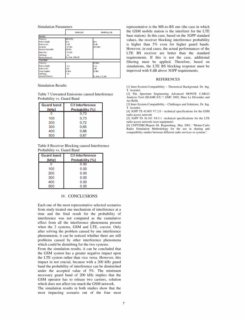
Table 7 Unwanted Emissions caused Interference
Probability vs. Guard Band
Table 8 Receiver Blocking caused Interference
Probability vs. Guard Band
IV. CONCLUSIONS
Each one of the most representative selected scenarios
from study treated one mechanism of interference at a
time and the final result for the probability of
interference was not computed as the cumulative
effect from all the interference phenomena present
when the 2 systems, GSM and LTE, coexist. Only
after solving the problem caused by one interference
phenomenon, it can be noticed whether there are still
problems caused by other interference phenomena
which could be disturbing for the two systems.
From the simulation results, it can be concluded that
the GSM system has a greater negative impact upon
the LTE system rather than vice versa. However, this
impact in not crucial, because with a 200 kHz guard
band the probability of interference can be diminished
under the accepted value of 5%. The minimum
necessary guard band of 200 kHz implies that the
GSM operator has to release two carriers, solution
which does not affect too much the GSM network.
The simulation results in both studies show that the
most impacting scenario out of the four most
representative is the MS-to-BS one (the case in which
the GSM mobile station is the interferer for the LTE
base station). In this case, based on the 3GPP standard
values, the receiver blocking interference probability
is higher than 5% even for higher guard bands.
However, in real cases, the actual performances of the
LTE BS receiver are better than the standard
requirements. If this is not the case, additional
filtering must be applied. Therefore, based on
simulations, the LTE BS blocking response must be
improved with 8 dB above 3GPP requirements.
REFERENCES
[1] Inter-System-Compatibility – Theoretical Background, Dr. Ing.
T. Asztalos
[2] The Spectrum Engineering Advanced MONTE CARLO Analysis Tool (SEAMCAT) *, EMC 2002, Marc Le Dévendec and
Ari Réfik
[3] Inter-System-Compatibility – Challenges and Solutions, Dr. Ing. T. Asztalos
[4] 3GPP TS 45.005 V7.2.0 – technical specifications for the GSM
radio access network
[5] 3GPP TS 36.101 V8.5.1 –technical specifications for the LTE
radio access network (user equipment)
[6] CEPT/ERC/Report 68, Regensburg, May 2001: “Monte-Carlo Radio Simulation Methodology for the use in sharing and
compatibility studies between different radio services or systems”.
7

Buletinul Ştiinţific al Universităţii Politehnica Timişoara
TRANSACTIONS on ELECTRONICS and COMMUNICATIONS
Volume 59(73), Issue 1, 2014
RAN Dimensioning for Wireless Networks
Razvan-Marius Popa Abstract – This paper paper will present the general
process of radio network design dimensioning and the
way the Vamos feature impacts dimensioning of the
Radio Access Network. The impact of VAMOS feature
over the Abis Interface dimensioning will be described.
Keywords: Abis, Vamos, capacity dimensioning
I. INTRODUCTION
The architecture of a 2G GSM network is presented in
Fig.1.
The Radio Access Network ( RAN ) is composed of
the BSC (Base Station Controller), the BTS (Base
Transceiver Station), the TC (Transcoder) and the
MFS (Multi-BSS Fast Packet Server) [1].
The BTS is a radio equipment which uses the radio
interface to receive and transmit information.A group
of BTS is handled by one BSC. The interface between
the BTS and the BSC is called Abis interface [2].
The BSC handles all associated radio functions like
RR management (for radio resource management and
mobility management during a call), power control,
handover, cell configuration data and channel
allocation. A group of BSC is served by a MSC
(Mobile Switching Center) and a SGSN (Serving
GPRS Service Node). Two interfaces leave the BSC:
Ater CS which is the interface conveying CS
information towards the transcoder (TC) and Ater PS
which is the interface conveying PS information
towards the MFS.
The transcoder can handle different types of codecs:
FR (Full Rate), EFR (Enhanced Full Rate), HR ( Half
Rate), AMR (Adaptive Multi Rate, transforms the
different coding into A law/miu law coding used in
the PCM format) and its major function is to translate
the 16 kbps channels called nibbles into 64 kbps
Fig. 1 GSM/GPRS/EDGE architecture[1]
channels called time slots (TS). The TC is linked to
the MSC by the A interface.
The MFS is in charge of performing the Packet
control function through the PCU (Packet Control
Unit).
The interface between the MSC and the SGSN is
called the Gb interface.
In this paper, the capacity dimensioning for the Abis
interface dimensioning for CS traffic coming from IP
sites will be detailed.
The capacity analysis is done independently from the
coverage analysis. Indeed the capacity of a cell, i.e.
the number of subscribers that can be handled,
depends only on:
- the user profile,
- the cell characteristics (i.e. how many TRXs
are available and in which configuration),
- the radio features that are available to boost
the capacity.
Also, it will be presented the impact of the VAMOS
feature over the dimensioning process of this
interface.
II. VAMOS FEATURE
VAMOS (Voice services over Adaptive Multi-user
channels on One Slot) is a 3GPP work item, the
objective of which is to specify a way in which two
users may be multiplexed on the same radio resource
simultaneously, i.e. using the same radio timeslot and
physical sub-channel.
In order to be able to use VAMOS, No new traffic
channels will be introduced to support VAMOS. The
existing FR and HR traffic channels will be used.
A. Downlink process
In the downlink direction, the BTS transmits
simultaneously to two MSs (Mobile Stations) on the
same frequency and TS, but using two different
training sequences, and a different modulation scheme
– alpha-Quadrature Phase Shift Keying (α -QPSK),
presented in “Fig. 2”[6], which allows two users to
share the same bandwidth, at the penalty of increased
interference.
In the diagram, two users are sharing the same
bandwidth, one using the first bit in each symbol, and
the other used the second. The value of α is chosen to
BTS
BTS
BTS
BSC MFS
SGSN
HLR
IP backbone
GGSN
PSTN
Internet/
Intranet
MSC/VLR
Mobile Radio
Mobile Core Circuit Switching
Mobile Core Packet Switching
TC
BTS
BTS
BTS
BSC MFS
SGSNSGSN
HLRHLR
IP backboneIP backbone
GGSNGGSN
PSTN
Internet/
Intranet
MSC/VLR
Mobile Radio
Mobile Core Circuit Switching
Mobile Core Packet Switching
TC
8

Fig. 2 α -QPSK diagram[7]
allow the power allocated to the two users to be
unequal.
α -QPSK can only be used when there is a 2-bit
symbol to transmit (one bit from each user).
Therefore, when DTX (Discontinuous Transmission)
is active, and there is a pause in speech from one user,
the other must switch back to using GMSK (Gaussian
Minimum Shift Keying, standard modulation scheme)
for the duration of the pause.
B. Uplink process
In the uplink direction, two MSs simultaneously
transmit their GMSK signal to the BTS on the same
TS and frequency. The BTS uses the different training
sequences to separate the signals (see Table 1).
Table 1 VAMOS Training sequences [6] Training
Sequence
Training sequence bits for the first set
0 (0,0,1,0,0,1,0,1,1,1,0,0,0,0,1,0,0,0,1,0,0,1,0,1,1,1)
1 (0,0,1,0,1,1,0,1,1,1,0,1,1,1,1,0,0,0,1,0,1,1,0,1,1,1)
2 (0,1,0,0,0,0,1,1,1,0,1,1,1,0,1,0,0,1,0,0,0,0,1,1,1,0)
3 (0,1,0,0,0,1,1,1,1,0,1,1,0,1,0,0,0,1,0,0,0,1,1,1,1,0)
4 (0,0,0,1,1,0,1,0,1,1,1,0,0,1,0,0,0,0,0,1,1,0,1,0,1,1)
5 (0,1,0,0,1,1,1,0,1,0,1,1,0,0,0,0,0,1,0,0,1,1,1,0,1,0)
6 (1,0,1,0,0,1,1,1,1,1,0,1,1,0,0,0,1,0,1,0,0,1,1,1,1,1)
7 (1,1,1,0,1,1,1,1,0,0,0,1,0,0,1,0,1,1,1,0,1,1,1,1,0,0)
Training sequence bits for the second set
0 (0,1,1,0,0,0,1,0,0,0,1,0,0,1,0,0,1,1,1,1,0,1,0,1,1,1)
1 (0,1,0,1,1,1,1,0,1,0,0,1,1,0,1,1,1,0,1,1,1,0,0,0,0,1)
2 (0,1,0,0,0,0,0,1,0,1,1,0,0,0,1,1,1,0,1,1,1,0,1,1,0,0)
3 (0,0,1,0,1,1,0,1,1,1,0,1,1,1,0,0,1,1,1,1,0,1,0,0,0,0)
4 (0,1,1,1,0,1,0,0,1,1,1,1,0,1,0,0,1,1,1,0,1,1,1,1,1,0)
5 (0,1,0,0,0,0,0,1,0,0,1,1,0,1,0,1,0,0,1,1,1,1,0,0,1,1)
6 (0,0,0,1,0,0,0,0,1,1,0,1,0,0,0,0,1,1,0,1,1,1,0,1,0,1)
7 (0,1,0,0,0,1,0,1,1,1,0,0,1,1,1,1,1,1,0,0,1,0,1,0,0,1)
III. BSS IP ARHITECTURES
The Abis interface conveys the CS traffic between the
BTS and the BSC. The transport mode that can be
used on this interface can be TDM or IP. Since the
VAMOS feature is available only with IP in the BSS,
only the 2 available IP architectures will be presented:
A. IP over Ethernet
Fig. 3 IPoEth architecture
The first architecture is called IP over Ethernet
(IPoEth) and offers a full IP over Ethernet solution.
The CS user plane flow that goes directly to the TC
and it is called the Abis CS flow. When dimensioning
the IP over Ethernet network the peak and the average
throughputs need to be computed.
B. IP over E1
Fig. 4 IPoE1 architecture
The second IP architecture is called IP over E1
(IPoE1). This architecture keeps the existing E1 links
on the Abis interface, and then introduces IP transport
within these links, using the Point-to-Point Protocol
(PPP) or the Multi Link PPP (ML-PPP) in the case of
two or more E1 links. The difference compared to the
previous architecture is the fact that the whole traffic
is routed towards the BSC. Beyond the BSC, the
logical flows are conveyed through the IP backbone.
The Ater CS flow is going form the BSC to the TC.
So, compared to the previous architecture, a new flow
appears.
IV. ABIS INTERFACE DIMENSIONING FOR CS
A. Information packing and headers
The CS traffic is carried on TRAU (Transcoder and
Rate Adaptation Unit) frames. One TRAU frame lasts
20 ms and is carried on the TDMA frames. The 20 ms
correspond to the duration of 4 TDMA frames.
Looking at the “Fig. 5”, it can be observed that a first
part of the TRAU frame is carried on TS1 of the 1st
Fig. 5 Multiplexing of TRAUP frames on IP packets
9

TDMA frame, the second part is carried also on TS1
of the second TDMA frame, the 3rd part of the TRAU
frame is carried on TS1 of the 3rd TDMA frame and
the last part of the TRAU frame is carried on TS1 of
the 4th TDMA frame. Finally, after 4 TDMA frames,
the whole TRAU frame is sent. The red TS
correspond to the 1st TRAU frame. A second TRAU
frame is carried on TS2 of each TDMA frame during
4 TD MA frames lasting 20 ms in the same way as the
1st one. In the figure above, the blue TS correspond to
the 2nd TRAU frame [7].
After the full TRAU frame is sent, it is put in an IP
packet. The IP packet contains only full TRAU
frames, in consequence only after the last part of the
TRAU frame has been received, it can be put in an IP
packet. Several TRAU frames are multiplexed over IP
packets. The TRAUP packets are composed out of
some useful information represented in the dark green
color and some headers represented in light green.
Inside the IP packet there are headers from each
protocol used: MUXTRAUP, UDP, IP and depending
on the architecture IPoEth or IPoE1 the Ethernet or
the [ML] PPP header is added.
When putting TRAUP frames into IP packets one of
the two limitations may occur before sending the IP
packet:
a) Maximum size supported by the IP packet
(MUXTRAUP_SIZE), which does not
include the Ethernet or the [ML] PPP header.
The typical size is 800 bytes [3].
b) Maximum time elapsed since beginning the
sending of TRAUP packets reflected in the
timer MAX_HOLD_MUXTRAUP. The
default value is 2 ms.
The IP packet is sent when encountering the first
limitation. If the delayed timer
MAX_HOLD_MUXTRAUP has expired then the
packet is sent even if it is not full, i.e. even if it didn’t
reach the maximum 800 bytes size.
These limitations will be carefully considered when
computing the number of IP packets needed to send
some information and the overheads associated to it.
The headers for IPoEth and IPoE1 are presented in
Table 2.
Table 2 IPoEth and IPoE1 headers [7]
PPP (Point-to-Point Protocol) HDLC is used in case
of a single E1 link on the Abis. In case of 2 or more
E1 links, [ML] PPP is used (Multi-link Point-to-Point
Protocol).
The TRAUP frame is built up as follows:
UL: 2 bytes (UL Address) + 1 byte (control) + N
bytes (payload, incl. 2 or 4 bits for the payload type)
[3]
DL: 2 bytes (Call-ID + DL Address) + 1 byte
(control) + N bytes (payload, incl. 2 or 4 bits for the
payload type) [3]
The payload depends on the codec. The values
considered in Alcatel-Lucent’s method[3] are:
a) TRAUP_Size FR = 244 bits
b) TRAUP_Size HR = 148 bits
B. IP Packets:
Headers associated to IP packets lead to overheads
and the number of IP headers depends on the number
of IP packets. In order to compute the overheads on
Abis introduced by all the protocol headers, the
number of IP packets need to be computed first.
The computation of the number of IP packets used to
carry CS traffic over 20 ms (TRAU frame duration)
depends then on the number of TRAU frames created
during T_MAX_HOLD_MUXTRAUP and the
maximum size of the IP packet.
The size of the information that can be put in an IP
packet during the timer
T_MAX_HOLD_MUXTRAUP is computed. This
will depend on the TRXs and the TS used for CS.
Information = N8 × TRAU× RoundDown T !"#$%&'()*&+timeslot/012345 6 (1)
With VAMOS, it is possible to carry 2 calls (i.e. 2
TRAU frames over 20ms) simultaneously on each
radio TS.
The number of calls will be doubled for a proportion
πVAMOS of the TS, and will remain as previously for a
proportion (1- πVAMOS).
Consequently, the number of TRAU frames, and also
the number of TRAUP bits, will change by
introducing a factor of:
(1- πVAMOS) + 2 × πVAMOS = [1 + πVAMOS] (2)
After the introduction of (2) in (1) we get:
:;<=>?@AB=;CDEF =GHIJ × (1 +LMNOPQ) × RSTUVWDXC ×roundDown YZ%*'!"#$%&'()*&+3[ \43]^_`abcd e(3)
The number of IP packets is the total information to
be carried divided by the maximum size of the blocks
used to carry that information. Or conversely, the
number of TS needed to be carried divided by the
number of TS corresponding to the Max_size. The
active TS, NCS to be sent are multiplied with the
VAMOS factor to account for the fact that with
VAMOS 2 calls are simultaneously carried on one TS.
IPoEth IPoE1
Header Size ( bytes )
Ethernet 38 -
[ML]PPP
HDLC
- 9 [13]
UDP/IP 28
MUXTRAUP 2
TRAUP Number_of_TRAUP_Frames *
TRAUP_Size
Total
(without
TRAUP)
68 39 [43]
10

Fig. 6 Number of IP Packets per 20 miliseconds
Fig. 7 VAMOS impact on Peak Throughput
The denominator represents the number of TS
corresponding to Max_size which is the maximum
size divided by the size of the TRAUP frame which
takes into account the HRCR and the different values
of the TRAUP frame for HR and FR. ghijklmnoHI= S=p;qUr gtQ × (1 +LMNOPQ)
S=p;qu=v; wTxQDEFyzSS × 2 × RSTUVQDEF~ +(1 − zSS) × RSTUQDEF6(4)
C. Peak Throughput
The CS peak throughput is the throughput reached
when all the CS radio TS are simultaneously active.
By multiplying the number of active TS used for CS
by the bitrate per TS, the figure obtained, Fig.7, is the
useful throughput for NCS TS. V@Rℎ>=pℎrpAtQ= gtQ× BAS@A × (1 − zSS) + 2× BAS@A × zSS× (1 +LMNOPQ)(5)
As it can be observed in the above chart the Peak
throughput increases rapidly with the VAMOS
penetration. For instance for a number of 180 active
TS the throughput achieved with VAMOS 100% is
more than double the one achieved without VAMOS.
D. Peak Overheads
The total CS overheads are computed by including
also the TRAUP headers (1 TRAUP header per active
call over 20 ms).The number of TRAUP frames in the
20ms period is doubled for the πPAIRED calls. >ℎ@qtQ = ghijklmnoHI × :VFFC +gtQ ×RSTUVFFC × (1 + LMNOPQ) × (1 + zSS)/20?(6)
Although the Peak overheads increase with the
VAMOS penetration (Fig. 8) - which is normal
Fig. 8 VAMOS influence on the Peak OH
Fig. 9 VAMOS influence on OH ratio
Fig. 10 VAMOS impact on Useful Average Throughput
considering that the more packets are sent during the
reference period, the more headers are sent, thus the
larger quantity of OH – the overhead ratio (Fig. 9)
computed as the overhead information reported to the
useful information tends to the same constant value no
matter the VAMOS penetration for large
configurations (more than 50 NCS).
E. Average Throughput
The Average throughput, Fig.10, is composed out of
the useful average throughput and the average
overheads. The average OH will be discussed in the
next paragraph. The useful average throughput is
impacted by the same [1 + πVAMOS] factor: U<pT>@Rℎ>=pℎrpA= BAS@A × (1 − zSS) + 2× BAS@A × zSS × (1
+ LMNOPQ) × (_)(7)F
Where ρcell represents the traffic intensity in the cell.
In the above charts, apart of the fact that the
throughput increases with the VAMOS penetration, it
is also that no major gain is brought by passing from
50% HRCR to 100% HRCR for the same penetration
of VAMOS (see light blue and dark blue lines), on the
other hand a significant improvement can be observed
when passing from VAMOS 0% to VAMOS 100%
for the same HRCR (see dark blue and pink lines).
Peak Overheads (kbps) IPoEth
0
200
400
600
800
1000
1200
1400
0 20 40 60 80 100 120 140 160 180
N_CS
IPo
Eth
Pe
ak
Overh
ead
s (
kb
ps)
(DT
X =
60%
, H
RC
R =
10
0%
)
VAMOS_0%
VAMOS_50%
VAMOS_100%
Peak Overheads (kbps) IPoEth
0
200
400
600
800
1000
1200
1400
0 20 40 60
Peak Overheads (kbps) IPoEth
0
200
400
600
800
1000
1200
1400
0 20 40 60 80 100 120 140 160 180
N_CS
IPo
Eth
Pe
ak
Overh
ead
s (
kb
ps)
(DT
X =
60%
, H
RC
R =
10
0%
)
VAMOS_0%
VAMOS_50%
VAMOS_100%
11

Furthermore, the impact on the average throughput is
a major one when considering both HRCR and
VAMOS 100%, the average throughput more than
doubles for the same number of NCS.
F. Average Overhead
For the average overhead computation, all the states in
which the system can be must be considered. The
following states and their corresponding probabilities
of occurrence must be considered: the state with 1
active call, with 2 active calls and so on up to NCS
active calls. For one specific state the computation is
the same as for the peak, but with NCS replaced by k
which can take values from 1 to NCS. The VAMOS
impact relies as for the peak in the number of IP
packets and the number of TRAUP frames transferred
during the 20ms period: >ℎ@qtQ() = ghijklmnoHI × :VFFC + × RSTUVFFC × (1 + LMNOPQ) × (1+ zSS)/20?(8)
An average overhead will be computed taking into
account all the overheads introduced by different
states and their probability of occurrence: T>@>ℎ@qtQ
=r()× >ℎ@qtQ()(9)
Since the average overhead computation is practically
based on the same formula as the peak overhead, the
same observations are valid, the overhead increases
with the NCS and also with the VAMOS proportion.
For the overhead ratio, although the overheads start
from a higher value for larger VAMOS penetration,
Fig. 11 VAMOS impact on Average Overhead
Fig. 12 VAMOS impact on Average Overhead Ratio
after a given configuration in terms of number of
active TS, the overhead ratio tends toward a constant
value no matter the VAMOS penetration.
V. CONCLUSIONS
VAMOS uses a new modulation, α-QPSK to allow
two voice calls to be transmitted simultaneously over
the same timeslot. This feature impacts the network
design dimensioning process in two of its branches:
Capacity and Abis dimensioning. A new parameter is
needed to account for the VAMOS impact, πVAMOS.
Abis Dimensioning requires changes to Number of IP
Packets computation, peak and average Overhead and
Throughput formulas to account for additional traffic
present. The influence relies on the [1 + πVAMOS]
factor which is explained by the fact that with
VAMOS, it is possible to carry 2 calls (i.e. 2 TRAU
frames over 20ms) simultaneously on each radio TS,
thus the number of calls will be doubled for a
proportion πVAMOS of the TS, and will remain as
previously for a proportion (1- πVAMOS).
Consequently, the number of TRAU frames in all the
previous formulas used in Abis dimensioning will
change by introducing a factor of (1- πVAMOS) + 2 *
πVAMOS = [1 + πVAMOS].
The effects of an increased VAMOS penetration on
Abis dimensioning are the increase of number of IP
packets that can be sent during the 20 ms period, the
increase of average and peak throughput but also the
increase of generated overheads which come from the
packet headers. All in all VAMOS brings a major
improvement since the throughput is larger and the
overall overhead ratio tends toward a constant figure
no matter the VAMOS penetration for a given number
of resources larger than 50 NCS.
REFERENCES
[1] M. Saily, G. Sebire, Dr. E. Riddington, “GSM/EDGE Evolution
and Performance”, John Wiley & Sons Ltd, 2011.
[2] M. Staiak, M. Glabowski, A.Wisniewski, P. Zwierzykowski,
“Modeling and Dimensioning of Mobile Networks – From GSM to
LTE”, John Wiley & Sons Ltd, 2011.
[3] “Capacity Analysis”, Alcatel-Lucent.
[4] E. Marza, “Comunicatii Mobile, note de curs”, Facultatea de Electronică şi Telecomunicaţii Timişoara, 2012.
[5] “Evolution of GSM voice”,
http://www.ericsson.com/res/docs/whitepapers/100716_VAMOS_a
pproved.pdf
[6] “Communication of redundant SACCH Slots during
discontinuous transmission mode for VAMOS”, http://www.faqs.org/patents/app/20110205947
[7] “GSM/GPRS/EDGE Radio Network design process for Alcatel-
Lucent BSS Release LR13”, Alcatel-Lucent.
12

Buletinul Ştiinţific al Universităţii Politehnica Timişoara
TRANSACTIONS on ELECTRONICS and COMMUNICATIONS
Volume 59(73), Issue 1, 2014
Carrier Aggregation in LTE-Advanced
Ioana-Elena Puşcaş 1
1 Faculty of Electronics and Telecommunications, Communications Dept.
Bd. V. Parvan 2, 300223 Timisoara, Romania, e-mail [email protected]
Abstract – LTE-Advanced extends the capabilities
originally defined in LTE within the 3GPP and Carrier
Aggregation (CA) is the most significant, although
complex, improvement provided by LTE-Advanced.
Bandwidths from various portion of spectrum are
logically concatenated or “aggregated” resulting in a
virtual block of a much larger band, enabling increased
data throughput. The aim of this paper is to present an
introduction of CA in LTE-Advanced system, including
current 3GPP status on CA technology, configuration
and deployment scenarios and Physical, MAC and RRC
(Radio Resource Control) Layers aspects of Carrier
Aggregation.
Keywords: LTE-Advanced, Carrier Aggregation, 3GPP
I. INTRODUCTION
LTE-Advanced (LTE-A) aims to support peak
data rates of 1 Gbps in the downlink and 500 Mbps in
uplink. [1] In order to fulfill such requirements, a
transmission bandwidth of up to 100 MHz is required.
However, since current versions of broadband
wireless systems make use of channel bandwidths of
up to 20 MHz the availability of such large portions of
contiguous spectrum is rare in practice. Therefore a
different spectrum management scheme is necessary
for next generation wireless systems in order to
achieve the required bandwidth.
LTE-Advanced uses carrier aggregation to form a
larger bandwidth by collection of multiple existing
carriers in order to meet the needs of higher
bandwidths. In Fig. 1 is presented CA concept in
LTE-Advanced system. [2] Each aggregated carrier is
referred to as a component carrier (CC). Release 8
LTE carriers have a maximum bandwidth of 20 MHz;
therefore LTE-Advanced can support aggregation of
up to five 20 MHz carriers.
Upon the demand on higher bandwidth and
higher data rate applications and based on the
expected growth of broadband users, LTE-Advanced
system introduced CA technology to overcome the
spectrum poverty and fragmentation problem,
irrespective of the peak data rate. [3]
Carrier aggregation in LTE-Advanced is designed
to support aggregation of a variety of different
arrangements of component carriers including carriers
of the same or different bandwidths, adjacent or non-
adjacent component carriers in the same frequency
band or in different frequency bands. [4] There are
three types of CA, depending on CC combinations:
a) Intra-band Contiguous CA
b) Inter-band Non-contiguous CA
c) Intra-band Non-contiguous CA
The component carrier can have a bandwidth of
1.4, 3, 5, 10, 15 or 20 MHz and, as mentioned earlier,
a maximum number of five component carriers can be
aggregated allowing for an overall transmission
bandwidth of up to 100 MHz. CA can be used for
both FDD and TDD. In FDD the number of
aggregated carriers can be different in downlink (DL)
and uplink (UL); however the number of UL
component carriers is always equal or lower that the
number of DL component carriers. The individual CC
can also be of different bandwidths. For TDD the
number of CCs as well as the bandwidths of each CC
will normally be the same for DL and UL.
Figure 2. Types of Carrier Aggregation
Figure 1. Concept of Carrier Aggregation
13

II. CONFIGURATION SCENARIOS OF CARRIER
AGGREGATION
3GPP has defined a range of carrier aggregation
scenarios for LTE-Advanced. Further we will present
five potential deployment CA scenarios considering
F1 and F2 two carriers to be aggregated (F2>F1). For
the DL all scenarios could be supported and for the
UL only scenarios #1, #2 and #3. [5]
A first possible CA configuration scenario is
described by following characteristics: F1 and F2
cells are co-located and overlaid, providing nearly the
same coverage. For this scenario both carriers are
generally within the same band (e.g. 2 GHz, 800
MHz, etc.) and it is expected that aggregation is
possible between overlaid F1 and F2 cells. [5]
The second possible scenario is similar with the
first one, F1 and F2 are co-located and overlaid, but
F2 has smaller coverage due to larger path loss. Only
F1 is used to provide full coverage and F2 is used to
further improve the data transfer rate for some
specific area. For this scenario the two carriers are
configured in different frequency bands (e.g. F1 =
800 MHz, 2 GHz and F2 = 3.5 GHz, etc.) and it
is expected that aggregation is possible between
overlaid F1 and F2 cells. [5]
In the third configuration scenario F1 and F2
cells are co-located, but F2 antennas are directed to
the cell boundaries of F1 to increase the throughput at
cell edge. In this configuration is also more likely that
the two carriers are configured in different frequency
bands. It is expected that F1 and F2 cells of the same
base station can be aggregated where coverage
overlap for higher data transmission rate. [5]
The fourth CA deployment scenario is shown in
Figure 5. F1 provides macro coverage and F2 is
deployed with Remote Radio Heads (RRHs) to
provide throughput at hot spots. Possible
configuration is to assign two carriers on different
frequency bands. It is expected that F2 cells can be
aggregated with the underlying F1 macro cells. [5]
The fifth configuration scenario is similar to
scenario #2, but frequency selective repeaters are
deployed so that coverage is extended for one of the
carrier frequencies. It is expected that F1 and F2 cells
of the same base station can be aggregated where
coverage overlap. [5]
III. PROTOCOL IMPACT OF CARRIER
AGGREGATION
Backward compatibility is essential for smooth
system migration and maximal reuse of the previous
design. The design of 3GPP LTE-Advanced carrier
aggregation considers backward compatibility; thus
CA feature enables concurrent data transmission on
multiple CCs, with procedures largely inherited from
LTE Release 8/9.
The services offered by higher layers are filled by
user plane and control plane function. The user plane
is responsible for data communicational, and the
control plane is responsible for maintaining the
connection between the network and the user
equipment (UE). The LTE R8/9 control plane stack
also applies to LTE-A CA. From the higher layer
viewpoint, each CC appears as a single cell with its
own cell identifier: each UE connects to one Primary
Serving Cell (Pcell) which is initially configured
during establishment and provides all necessary
control information and functions; besides, up to four
Secondary Serving Cells (SCells) may be configured
after connection establishment only to provide
additional radio resources. [6]
Figure 3. CA deployment scenario #1
Figure 4. CA deployment scenario #2
Figure 6. CA deployment scenario #4
Figure 5. CA deployment scenario #3
Figure 7. CA deployment scenario #5
14

In the user plane protocol design for LTE-A, the
use of carrier aggregation is not visible above the
Medium Access Control (MAC) layer.
A. Physical Layer Aspects
The exchanging of the data and control
information between network and UE is the
responsibility of the physical layer. LTE-A CA
inherits the legacy LTE data transmission per CC,
including multiple access scheme, modulation and
channel coding (MCS). Additional UE functionalities
are supported in LTE-A, but the main challenge in the
design of CA was improving the DL and UL control
signaling to efficiently support data transmission. [7]
For downlink, at the start of each subframe of
each DL CC a control region is available for Physical
Control Format Indicator Channel (PCFICH –
transmits a control format indicator, CIF, field which
specifies the number of OFDMA symbols carrying
control information), Physical Downlink Control
Channel (PDCCH – supports information on resource
allocation, MCC, HARQ etc.) and Physical HARQ
Indicator Channel (PHICH – used for transmission of
the HARQ ACK/NACKs).
A key characteristic of CA is a cross-carrier-
scheduling. This enables a PDCCH on a CC to be
configured in order to scheduled PDSCH and PUSCH
transmissions on other CCs by means of new 3-bits
carrier indicator field (CIF) inserted at the beginning
of the PDCCH. The main motivation for cross-carrier
scheduling is to support Inter-Cell Interference
Coordination (ICIC) for PDCCH in heterogeneous
networks, so CA can reduce or even eliminate ICIC
on PDCCH of the CC which can schedule data
resources on others CCs and improve data rates. [8]
The normal scheduling operation where the
PDCCH with the corresponding PDSCH or PUSCH
are transmitted on the same cell is also maintained for
backward compatibility. It is possible to transmit
PDCCH scheduling a PDSCH on the same carrier
frequency and PDCCH scheduling a PUSCH on a
linked UL carrier frequency where the linkage of the
DL and UL carriers in conveyed as system
information.
Based on the decoded CFI value, UE derives the
starting point of PDSCH transmission. In the case of
PDSCH non-cross-carrier scheduled by PDCCH on
the same component carrier, UE is required to decode
the PCFICH in order to determine the starting OFDM
symbol used for PDSCH. For PDSCH cross-carrier
scheduled by PDCCH on another carrier, the starting
OFDM symbol for PDSCH transmission is configured
by the network though higher layers, and the UE is
not required to decode the PCFICH on the CC of the
PDSCH transmission. [9]
The design of the PHICH in LTE-Advanced CA
follows the design of LTE Release 8.
Uplink control signaling, UCI, includes HARQ
ACK/NACK signaling corresponding to potentially
multiple PDSCHs, scheduling requests and Channel
State Information (CSI). As in LTE Release 8/9, UCI
can be transmitted on a physical uplink control
channel (PUCCH) if there is no transmission on a
PUSCH in a subframe, and transmitted on PUSCH
otherwise. LTE-Advanced further supports, by
network configuration, simultaneous transmission of
PUCCH and PUSCH in a sub frame. This allows the
base station to flexibly control the performance of the
PUCCH and PUSCH independently and to avoid the
UCI overhead on the PUSCH by utilizing existing
PUCCH resources. The PUCCH can only be
transmitted on the PCell, since it typically has more
reliable link quality and coverage relative to the
SCells. When applicable, UCI is always transmitted
on a single PUSCH. [9]
LTE Release 8/9 PUCCH known as format 1b
was only defined to support up to 4 bits (2 bits in FFD
and 4 bits in TDD), so HARQ feedback can only be
transmitted only for two CCs. The PUCCH format 3
was introduced in LTE-A to support HARQ feedback
for a UE configured with downlink CA. This enables
a full range of ACK/NACK bits to be transmitted (up
to 10 Bits for FDD and up to 20 bits in TDD). [7]
Channel state information (CSI) feedback assist
the network to achieve PDSCH scheduling, including
resource selection, MCS selection, transmission rack
indicator and precoding matrix indicator. In order to
handle the different channel conditions and interface
level among different CCs, the CSI is configured for
each CC. In LTE-Advanced, both periodic and
aperiodic CSI feedbacks are supported. LTE-
Advanced supports aperiodic CSI feedback for a
single or multiple CCs in a subframe in order to
balance the CSI accuracy and feedback overhead. [9]
In CA, periodic CSI is reported for only one CC
in a subframe. Different offsets and periodicities
should be configured to minimize collisions between
CSI reports of different CCs in a subframe. In case the
collisions involve the multiple periodic CSI reports,
the priority is according to defined prioritization rules.
Aperiodic CSI feedback is transmitted on PUSCH and
carries more CSI than periodic CSI feedback. In the
case of a collision between periodic and aperiodic CSI
for downlink CCs, the periodic CSI is dropped. [7]
B. MAC Layer Aspects
From the MAC perspective the CA simply
provides additional conduits, thus the MAC layer
Figure 8. Cross-carrier scheduling
15

plays the role of a multiplexing entity for the
aggregated components carriers. [10] There is one
MAC entity per user, which controls the multiplexing
of data from all logical channels to the user, and
further controls how this data is transmitted on the
available CCs. Each MAC entity will provide to his
corresponding CC its own Physical Layer entity,
providing resource mapping, data modulation, HARQ
and channel coding.
The interface between the MAC layer and the
physical layer, which are referred to as transport
channels, is also separate for each component carrier.
[8]
V. CONCLUSIONS
This article provides an overview of CA in 3GPP
LTE-Advanced. CA for LTE-Advanced is fully
backward compatible, which essentially means that
legacy LTE Release 8/9 terminals and LTE-Advanced
terminals can co-exist maintaining the advantages of
legacy technologies and reducing the cost per bit and
saving energy.
Carrier Aggregation has much more to offer and
it continues to be a significant area of work for 3GPP,
equipment manufacturers and network operators and
will continue to be one of the most important
techniques in the next generation telecommunication
system. Over the coming years there will be a
number of important developments, including, for
example: increasing the number of CCs and the total
bandwidth supported in both the DL and the UL;
supporting a greater number of frequency bands and
combinations of frequency bands; supporting CA
between licensed and unlicensed spectrum. [13]
REFERENCES
[1] 3GPP Technical Report 36.913, “Requirements for further
advancements for Evolved Universal Terrestrial Radio Access (E-
UTRA) (LTE-Advanced)”, www.3gpp.org.
[2] E. Seidel, “LTE-A Carrier Aggregation Enhancements in
Release 11”, NOMOR Research GmbH, Munich, Germany, 2012.
[3] A. Z. Yonis, M. F. L. Abdullah, M. F. Ghanim, “Effective Carrier Aggregation on the LTE-Advanced Systems”, International
Journal of Advanced Science and Technology, vol. 41, April, 2012.
[4] 3GPP documentation - Carrier Aggregation explained
http://www.3gpp.org/technologies/keywords-acronyms/101-carrier-
aggregation-explained
[5] 3GPP Technical Report R2-102490, “CA deployment scenarios,” NTT DOCOMO, INC.
[6] Z. Shen, A. Papasakellariou, J. Montojo, D. Gerstenberger, F.
Xu, „Overview of 3GPP LTE-Advanced Carrier Aggregation for
4G Wireless Communications“, IEEE Magazine, February, 2012.
[7] M. Al-Shibly, M. Habaebi, J. Chebil, “Carrier Aggregation in
Long Term Evolution- Advanced”, IEEE Control and System Graduate Research Colloquium, 2012.
[8] S. Ahmadi, “LTE-Advanced: A Practical System Approach to
Understanding the 3GPP LTE Releases 10 and 11 Radio Access Technologies”, Elsvier Science and technology Books, UK, 2014.
[9] H. Holma, A. Toskala,“LTE-Advanced: 3GPP Solution for
IMT-Advanced“, John Wiley& Sons, Inc., 2012
[10] Anritsu - Understanding LTE-Advanced Carrier Aggregation
https://www.anritsu.com/en-GB/Promotions/carrier-aggregation-
guide/registration.aspx [11] F. Ren, C. Wang, A. Chen, W. Sheen, „Introduction to Carrier
Aggregation Technology in LTE-Advanced Systems“, International
Conference on Advanced Information Technologies, 2011
[12] http://www.artizanetworks.com/lte_tut_adv_acceleration.html
[13] http://www.unwiredinsight.com/2014/lte-carrier-aggregation-
evolution
Figure 9. Downlink MAC Layer structure with CA
16

Buletinul Ştiinţific al Universităţii Politehnica Timişoara
TRANSACTIONS on ELECTRONICS and COMMUNICATIONS
Volume 59(73), Issue 1, 2014
Telemetric Applications for the Automotive Industry using IQRF
devices
Victor Serban, Dan Andreiciuc, Aurel Filip
Abstract— The proposed system implies exploiting a
technology previously utilized in smart home automation, namely
IQRF boards, in the automotive industry. Employing these
devices, one can obtain a more versatile control of his/her vehicle,
as well as various aspects of environmental conditions, like
temperature or the intensity of light outside the vehicle. This
system constitutes of a modular hardware part, and multiple
software parts, each accomplishing some of the previously
enumerated notions. (Abstract)
Keywords—IQRF; Automotive; IQMESH; Telemetry (key words)
I. INTRODUCTION
IQRF is a sub GHz wireless communications technology. It is
intended where wireless general use connectivity is needed, be
it point to point, or in complex networks. Its functionality
depends only on a dedicated application written in the C
programming language.
The object of this application that is presented in this paper is
the integration of smart house applications in the automotive
industry.
The elementary IQRF communication is the transceiver
module including a microcontroller with an onboard operating
system, implementing the physical level, as well as the data
link level upholding the MESH network which utilizes the
open IQMESH protocol. No other superior level, like the
transport level is part of this technology.
II. IQRF MODULAR HARDWARE UTILIZED
IQRF Technology Characteristics
Among the main properties of the IQRF technology are: low speeds, low power consumption and low data rate, packet based oriented data radio frequency up to 128 Bits/packet, RF software selectable parameters, sub-GHz radio frequency bands using multi canal systems and FSK modulation, bit rate between 1,2 – 86,2kb/s, output power of maximum 20mW, output range of over 1 Km per hop, up to 240 hops per packet, up to 65000 devices in a single network, low power consumption (380nA in idle mode and 25 uA when receiving), the code can be uploaded wirelessly to all nodes in the same time and last but not least, there is no license acquisition fee.
III. HARDWARE CHARACTERISTICS
A. DK-EVAL-04
The DK-EVAL-04 is a universal development kit for wireless
IQRF transceivers. Its reduced size, LiPol accumulator and low
cost make this kit ideal for intelligent network application
usage.
Applications for this device include: the development of
wireless applications, host for TR IQRF modules, testing and
debugging of IQMESH networks and portable battery powered
wireless systems.
The simplified diagram of the board is presented in Fig.1.
B. CK-USB-04
The CK-USB-04 is a development kit oriented towards the
programming and debugging of user applications with IQRF
transceivers. It can also serve as a IQRF USB gateway (USB –
SPI converter) or just a simple host for the transceiver module.
Among the key applications are the following: programmer
board for the IQRF transceiver, IQRF debug kit, final IQRF
application host, USB host, USB – SPI converter and finally
PC connectivity. The simplified circuit diagram is presented in the Fig.2.
Fig.1 – Simplified diagram of the DK-EVAL-04 board
17

Fig.2 – Simplified diagram for the CK-USB-04 board
The network can be controlled using three words:
1. Node address
2. Peripheral number – indicates with which peripheral I can communicate with
3. Each peripheral number has different commands
Each packet can have 58 bits that can be used.
C. SHD-SE-01
The SHD-SE-01 is a multifunctional wireless sensor that gives
temperature readings, illumination, acceleration measurement,
has a real time clock as well as an EEPROM memory.
Its low power usage design allows its battery to last for years
on end.
The sensor can be adapted to user specific functionality
through application software for the microcontroller in the
operating system included transceiver module.
The key characteristics of the sensor are the following: smart
Transceiver station with built-in antenna, Selectable band of
FR 868 / 916 MHz with multiple channels, internal
microcontroller equipped with an operating system, compatible
with TR-54D, 3 axis accelerometer, temperature sensor, light
sensor, real time clock, serial EEPROM, tactile button, LED
indicator, ultra reduced power consumption, integrated primary
battery with a multi-year lifetime and a programmable
application in the internal transceiver module.
Fig.3 represents a picture of the SHD-SE-01 module.
Fig.4 will represent the simplified block diagram of the SHD-
SE-01 module.
Fig.3 Image of the SHD-SE-01 module
Fig.4 Simplified block diagram of the SHD-SE-01 module
IV. SOFTWARE ARCHITECTURE
Software architecture is defined by IEEE as: basic organization
of a system embodied in the system components, the
relationships between them and between system components
and the environment, and the principles governing the design
and evolution of the system. [ANSI/IEEE Std. 1471-2000,
Recommended Practice for Architectural Description of
Software-Intensive Systems].
The definition proposed by IEEE says that architecture
captures system structure in terms of its components and how
these components interact. The system architecture defines the
rules by which the system is designed as well as defining how
it can be changed.
An embedded enterprise architecture is organized in four
levels:
• drivers working with hardware (its abstraction).
• Basic Software - eg AdcHandler (mode like reading
series features several ADC channels, applying
transformations on the results).
• OS - basic skeleton of an operating system based on
tasks (model time-slice).
• Application - Module generic state machines,
controllers, error checking, etc.
18
This type of architecture is commonly used in automotive
industry. The proposed variant satisfies the portability and
future expansion, given the requirements and the complexity of
the application.
To demonstrate the feasibility of using IQRF devices, but also
to have a starting point for the concept car telemetry
integration in smart home, they realized some projects in the
IQRF IDE 4.7. The first project aims to familiarize with the
programming environment, the operating system and the
attached framework and programming devices and using
IQRF.
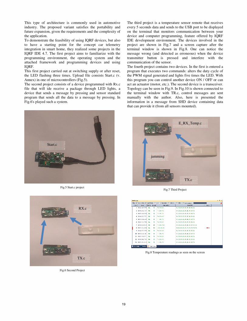
This first project carried out at switching supply or after reset,
the LED flashing three times. Upload file consists Start.c (v.
Annex) in one of microcontrollers (Fig.5).
The second project consists of a device programmed with Rx.c
file that will ide receive a package through LED lights, a
device that sends a message by pressing and sensor standard
program that sends all the data to a message by pressing. In
Fig.6's played such a system.
Fig.5 Start.c project
Fig.6 Second Project
The third project is a temperature sensor remote that receives
every 5 seconds data and sends to the USB port to be displayed
on the terminal that monitors communication between your
device and computer programming, feature offered by IQRF
IDE development environment. The devices involved in the
project are shown in Fig.7 and a screen capture after the
terminal window is shown in Fig.8. One can notice the
message wrong (and detected as erroneous) when the device
transmitter button is pressed and interfere with the
communication of the sensor.
The fourth project contains two devices. In the first is entered a
program that executes two commands: alters the duty cycle of
the PWM signal generated and lights five times the LED. With
this program you can control another device ON / OFF or can
act an actuator (motor, etc.). The second device is a transceiver.
Topology can be seen in Fig.9. In Fig.10 is shown connected to
the terminal window with TR.c, control messages are sent
manually with the author. Also, here is presented the
information in a message from SHD device containing data
that can provide it (from all sensors mounted).
Fig.7 Third Project
Fig.8 Temperature readings as seen on the screen
Start.c
E_RX_Temp.c
jamming
TX.c
TX.c
RX.c
19

Fig.9 The fourth project
Fig.10 Terminal window, message transmission and reception
Fig.11 – The fifth Project
The last project contains an interpretation program of the
messages coming from the SHD. The implementation is seen
in Fig.11. This program can be directly used to monitor the
automobile. Thus, alarms can be set if the vehicle is moved,
started, what temperature is inside, etc. Commands can be
sent, as seen in the previous project to lock the doors, stop the
engine, start the air conditioning, etc. The car will be as such
in a permanent state of monitoring and control.
One utility example can be seen when a person wants to leave
home in an hour. This is signaled to the smart house intelligent
system, which verifies the temperature in the car and in case it
is too high, turns on the air conditioning. In such a way the
vehicle will be ready for the voyage.
V. CONCLUSIONS
In the proposed paper is presented the exploitation of a
technology that until recently was used only in the smart home.
The idea to gather telemetry from inside a car is also an
innovative one not implemented by the time of the current
study.
The programs used in the C programming language are simple,
with no great complexity and can be easily carried, debugged
and tested.
The sensors have a battery life of several years, providing a
long and independent functionality comparable to the average
user to overhaul a car.
We can advance the application on IQRF devices in cars by
manipulating a visual control panel touchscreen display that
can receive both data and sensor nodes and monitor activity
programs running in them, besides work and monitor the
integrated smart home.
ACKNOWLEDGMENT
This work was partially supported by the Polithenica University of Timisoara, Department of Applied Electronics with the assistance of Assoc. Prof. Dr. Eng. Dan Andreiciuc.
REFERENCES
[1] APLICAȚII TELEMETRICE PENTRU INDUSTRIA AUTOMOTIVE
UTILIZÂND DISPOZITIVE IQRF, Serban Victor
[2] ***, http://en.wikipedia.org/wiki/Telemetry
[3] ***, http://en.wikipedia.org/wiki/Wireless_sensor_network
[4] ***, IQRF Quick Start Guide,
http://www.iqrf.org/weben/index.php?sekce=support&id=download
[5] ***, IQRF Technical Guide,
http://www.iqrf.org/weben/index.php?sekce=support&id=download
[6] ***, DK-EVAL-04 User’s Guide,
http://www.iqrf.org/weben/index.php?sekce=support&id=download
[7] ***, CK-USB-04 User’s Guide,
http://www.iqrf.org/weben/index.php?sekce=support&id=download
[8] ***, SHD-SE-01 User’s Guide,
http://www.iqrf.org/weben/index.php?sekce=support&id=download
[9] ***, Wikipedia, http://en.wikipedia.org/wiki/IQRF
[10] ***, SOS Electronic Webinar, http://www.soselectronic.com/?str=1426
[11]. Brian Kernighan and Dennis Ritchie, The C Programming Language,
1978 (1st edition), Englewood Cliffs, NJ: Prentice Hall. ISBN 0-13-110163-3.
TR.c
multi_com.c
prel_msg_SHD.
20

Buletinul Ştiinţific al Universităţii Politehnica Timişoara
TRANSACTIONS on ELECTRONICS and COMMUNICATIONS
Volume 59(73), Issue 1, 2014
Multifunctional Siren for Emergency Services
Cătălin Tudoran1 Dan Andreiciuc
2 Aurel Filip
3
1 E-mail [email protected] 2 Faculty of Electronics and Telecommunications, Applied Electronics Dept., Bd. V. Pârvan, 300223 Timisoara, Romania, e-mail [email protected] 3 Faculty of Electronics and Telecommunications, Applied Electronics Dept., Bd. V. Pârvan, 300223 Timisoara, Romania, e-mail
Abstract – this paper presents a solution for the design
of a multifunctional siren for emergency services (police,
ambulance, special services etc). Such a device should
have two functionalities: both as a voice amplifier and as
a tone generator. When designing such a circuit, a D
class amplifier has been considered for the amplification
and a PIC microcontroller for the tone generation. A
switch should be used to interchange these
functionalities and user buttons must be provided for
configuring the tone libraries.
Keywords: siren, class D amplifier, PIC, microcontroller
I. INTRODUCTION
From the beginning of time, sounds have been used
by every living being on this planed as a means of
communication. By means of sounds we can
communicate almost everything, from simple words
to tones used in warning systems. From the physical
point of view, sound is a vibration that propagates as a
typically audible mechanical wave of pressure and
displacement, through a medium such as air, and
water. In physiology and psychology, sound is the
reception of such waves and their perception by the
brain. Sound waves are often simplified to a
description in terms of sinusoidal plane waves, which
are characterized by the following properties:
frequency, wavelength, wavenumber, amplitude,
sound pressure, sound intensity, speed of sound and
direction. The human ear can only perceive sounds
with frequencies between 20 Hz and 20 kHz with a
maximum audibility around 3500 Hz. This interval is
mainly influenced by the amplitude of the vibrations
and the age and health of the individual.
II. POWER AMPLIFIERS
An audio power amplifier is an electronic amplifier
that amplifies low-power audio signals (signals
composed primarily of frequencies between 20 - 20
000 Hz, the human range of hearing) to a level
suitable for driving loudspeakers. It is the final
electronic stage in a typical audio playback chain.
Because power amplifiers are large-signal amplifiers,
a much larger portion of the load line is used during
signal operation than in a small-signal amplifier.
There are a few basic classes of power amplifiers:
class A, class B, class AB, class C and class D. These
amplifier classifications are based on the percentage
of the input cycle for which the amplifier operates in
its linear region. Each class has a unique circuit
configuration because of the way it must be operated.
The emphasis is on power amplification. Power
amplifiers are normally used as the final stage of a
communications receiver or transmitter to provide
signal power to speakers or to a transmitting antenna.
Fig.1. Basic example of a power amplifier, where:
− η% is the efficiency of the amplifier.
− Pout is the amplifiers output power delivered to the load.
− Pdc is the DC power taken from the supply.
A. Class A amplifiers
The Class A amplifier is the most common and
simplest form of power amplifier that uses the
switching transistor in the standard common emitter
circuit configuration. The transistor is always biased
“ON” so that it conducts during one complete cycle of
the input signal waveform producing minimum
distortion and maximum amplitude to the output.
Both large-signal and small-signal amplifiers are
considered to be class A if they operate in the linear
region at all times. Class A power amplifiers are
large-signal amplifiers with the objective of providing
power (rather than voltage) to a load. As a rule of
thumb, an amplifier may be considered to be a power
amplifier if it is rated for more than 1 W and it is
necessary to consider the problem of heat dissipation
21
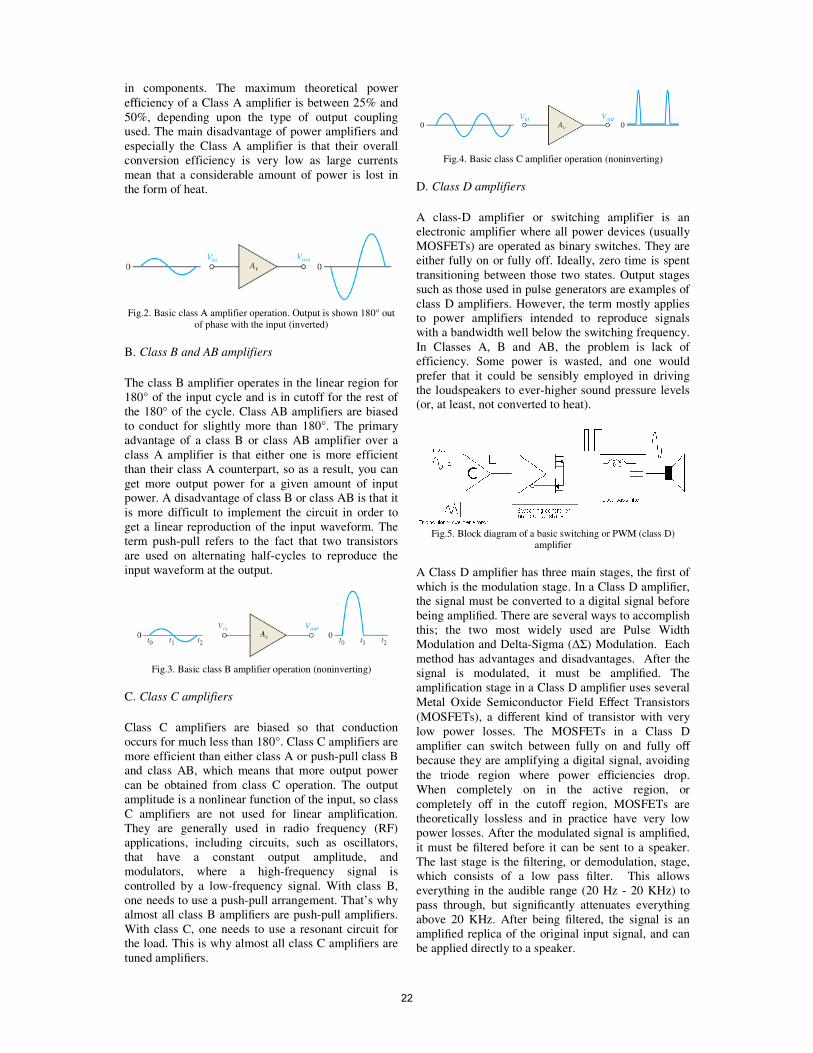
in components. The maximum theoretical power
efficiency of a Class A amplifier is between 25% and
50%, depending upon the type of output coupling
used. The main disadvantage of power amplifiers and
especially the Class A amplifier is that their overall
conversion efficiency is very low as large currents
mean that a considerable amount of power is lost in
the form of heat.
Fig.2. Basic class A amplifier operation. Output is shown 180° out
of phase with the input (inverted)
B. Class B and AB amplifiers
The class B amplifier operates in the linear region for
180° of the input cycle and is in cutoff for the rest of
the 180° of the cycle. Class AB amplifiers are biased
to conduct for slightly more than 180°. The primary
advantage of a class B or class AB amplifier over a
class A amplifier is that either one is more efficient
than their class A counterpart, so as a result, you can
get more output power for a given amount of input
power. A disadvantage of class B or class AB is that it
is more difficult to implement the circuit in order to
get a linear reproduction of the input waveform. The
term push-pull refers to the fact that two transistors
are used on alternating half-cycles to reproduce the
input waveform at the output.
Fig.3. Basic class B amplifier operation (noninverting)
C. Class C amplifiers
Class C amplifiers are biased so that conduction
occurs for much less than 180°. Class C amplifiers are
more efficient than either class A or push-pull class B
and class AB, which means that more output power
can be obtained from class C operation. The output
amplitude is a nonlinear function of the input, so class
C amplifiers are not used for linear amplification.
They are generally used in radio frequency (RF)
applications, including circuits, such as oscillators,
that have a constant output amplitude, and
modulators, where a high-frequency signal is
controlled by a low-frequency signal. With class B,
one needs to use a push-pull arrangement. That’s why
almost all class B amplifiers are push-pull amplifiers.
With class C, one needs to use a resonant circuit for
the load. This is why almost all class C amplifiers are
tuned amplifiers.
Fig.4. Basic class C amplifier operation (noninverting)
D. Class D amplifiers
A class-D amplifier or switching amplifier is an
electronic amplifier where all power devices (usually
MOSFETs) are operated as binary switches. They are
either fully on or fully off. Ideally, zero time is spent
transitioning between those two states. Output stages
such as those used in pulse generators are examples of
class D amplifiers. However, the term mostly applies
to power amplifiers intended to reproduce signals
with a bandwidth well below the switching frequency.
In Classes A, B and AB, the problem is lack of
efficiency. Some power is wasted, and one would
prefer that it could be sensibly employed in driving
the loudspeakers to ever-higher sound pressure levels
(or, at least, not converted to heat).
Fig.5. Block diagram of a basic switching or PWM (class D)
amplifier
A Class D amplifier has three main stages, the first of
which is the modulation stage. In a Class D amplifier,
the signal must be converted to a digital signal before
being amplified. There are several ways to accomplish
this; the two most widely used are Pulse Width
Modulation and Delta-Sigma (∆Σ) Modulation. Each
method has advantages and disadvantages. After the
signal is modulated, it must be amplified. The
amplification stage in a Class D amplifier uses several
Metal Oxide Semiconductor Field Effect Transistors
(MOSFETs), a different kind of transistor with very
low power losses. The MOSFETs in a Class D
amplifier can switch between fully on and fully off
because they are amplifying a digital signal, avoiding
the triode region where power efficiencies drop.
When completely on in the active region, or
completely off in the cutoff region, MOSFETs are
theoretically lossless and in practice have very low
power losses. After the modulated signal is amplified,
it must be filtered before it can be sent to a speaker.
The last stage is the filtering, or demodulation, stage,
which consists of a low pass filter. This allows
everything in the audible range (20 Hz - 20 KHz) to
pass through, but significantly attenuates everything
above 20 KHz. After being filtered, the signal is an
amplified replica of the original input signal, and can
be applied directly to a speaker.
22

What generally happens in class D amplifiers is that
that the transistors switch alternately to lift the output
all the way up to the positive supply rail, then all the
way down to the negative supply rail, as quickly as
possible, with no in-between voltages. This is clearly
going to be a pulse waveform. The secret to class D is
that if the width of the pulses can be made
proportional to the input signal's instantaneous level,
the power delivered to the loudspeaker, averaged over
time, will be the same as if the input signal had been
amplified in the conventional way.
Fig.6. Class D amplifier waveforms
Generally speaking, class D amplification is achieved
by modulating a signal, amplifying the modulated
signal and then filtering the amplified signal back into
its original form. Since Class D amplifiers work with
digital signals, they do not require that the transistors
involved operate in the triode region and, as a result,
they are much more efficient than other amplifiers.
This method of amplification has been used in
portable audio devices, cell phones and low fidelity
audio where size, power and heat dissipation are of
great concern. The advantages of Class D, however,
can also be applied to the larger systems required for
live audio. The reduction in power consumption made
possible by a Class D system is sometimes considered
unnecessary for live audio because the size and
efficiency of an audio system is not usually a concern
when the system is permanently installed in a venue
and the power is drawn from the wall. In our case,
however, when we are speaking about emergency
services and cars equipped with sirens and voice
amplifiers, this advantage becomes very attractive.
Class D amplifiers have historically only been used in
a limited number of applications, like motor control,
because it is more difficult to generate the high quality
signals required for audio applications with a Class D
amplifier. Recently, however, Class D technology has
advanced sufficiently to allow these amplifiers to
accurately and cleanly amplify audio signals. There
are many advantages to using Class D amplifiers for
audio applications, and the number of disadvantages
is shrinking every year with further advances in
technology.
III. ADVANTAGES AND DISADVANTAGES
OF CLASS D AMPLIFIERS
Further on, some advantages and disadvantages of
Class D amplifiers will be presented. Despite the
complexity involved, a properly designed class D
amplifier offers the following benefits:
− reduced power waste as heat dissipation
− because of the above, a reduction in cost, size and
weight of the amplifier due to smaller (or no) heat
sinks, and compact circuitry
− very high power conversion efficiency, usually
better than 90% above one quarter of the
amplifier's maximum power, and around 50% at
low power levels.
While Class D amplifiers have been in use for many
years, only recently have they come to the forefront of
audio amplification. This is because Class D
amplifiers have a number of disadvantages that make
them less suitable for audio amplification, though
many of these have been overcome with recent
advances in technology. One major disadvantage is
that a Class D amplifier has a very high amount of
high frequency noise, generated by the switching
design. This noise must be kept at a high enough
frequency to be inaudible, yet to a minimum
amplitude to meet Federal Communications
Commission (FCC) regulations. To help reduce
extraneous noise, a filter is added after the amplifying
stage. This filter is an additional component of the
Class D amplifier, and adds complexity, weight, and
cost. The added weight is negligible, however, when
compared to the weight of the heat sink required for a
Class A, Class AB or Class B amplifier. The
additional cost of a filter may also be minimized using
careful design techniques. Since the filter only needs
to attenuate signals above the audible frequencies, it is
not essential that the filter be extremely precise. The
filter may therefore be realized by a fairly simple,
low-pass, passive filter.
A second deficiency of Class D amplifiers is the
increased complexity in design. This may result in
increased design time and expense. Increased design
expenses are generally considered acceptable,
however, if the result is a lower manufacturing cost
because design is singular expense, whereas
manufacturing expenses are recurring. After the
amplifier is designed, most of the components, with
the possible exception of any inductors used in the
filter and specialized MOSFETs in the power stage,
are extremely inexpensive when purchased in bulk.
So while the increased complexity seems like a major
disadvantage, it may become irrelevant when the
amplifiers are mass-produced.
The last major disadvantage of Class D amplifiers is
that historically, distortion has been a major problem.
High Total Harmonic Distortion (THD) is indicative
of high noise levels, which detract significantly from
the audio quality of the output. Advances in
technology have allowed for faster modulation
23

techniques, however, which can reduce THD to
fractions of a percentage in Class D audio amplifiers.
After consideration of advantages and disadvantages,
the conclusion would be that such a Class D amplifier
is ideal for use in vehicles and especially when
equipping it for emergency services. Because of the
light weight, low power consumption and relatively
high quality output, it would serve the purpose of this
project.
IV. THE TDA7498 AMPLIFIER
The TDA7498 is a dual BTL class-D audio amplifier
with single power supply designed for home systems
and active speaker applications. It comes in a 36-pin
PowerSSO package with exposed pad up (EPU) to
facilitate mounting a separate heat sink. Some of its
features are described below:
− 100 W + 100 W output power at THD = 10%
with RL = 6 Ω and VCC = 36 V
− 80 W + 80 W output power at THD = 10% with
RL = 8 Ω and VCC = 34 V
− Wide range single supply operation (14 - 39 V)
− High efficiency (η = 90%)
− Four selectable, fixed gain settings of nominally
25.6 dB, 31.6 dB, 35.1 dB and 37.6 dB
− Differential inputs minimize common-mode noise
− Standby and mute features
− Short-circuit protection
− Thermal overload protection
− Externally synchronizable
Such a device will have as input a microphone (for
example, a CB Mic, because it has buttons for on/off
and is portable) and as output, the loudspeakers. The
device will amplify the sounds coming from the
microphone when necessary.
V. THE PIC16F84A MICROCONTROLLER
The PIC16F84A is an 18-pin Enhanced
FLASH/EEPROM 8-Bit Microcontroller. It belongs
to the mid-range family of the PICmicro®
microcontroller devices. Some of the features are
described below:
A. High Performance RISC CPU Features
• Only 35 single word instructions to learn
• All instructions single-cycle except for program
branches which are two-cycle
• Operating speed: DC - 20 MHz clock input DC -
200 ns instruction cycle
• 1024 words of program memory
• 68 bytes of Data RAM
• 64 bytes of Data EEPROM
• 14-bit wide instruction words
• 8-bit wide data bytes
• 15 Special Function Hardware registers
• Eight-level deep hardware stack
• Direct, indirect and relative addressing modes
• Four interrupt sources:
- External RB0/INT pin
- TMR0 timer overflow
- PORTB<7:4> interrupt-on-change
- Data EEPROM write complete
B. Peripheral Features
• 13 I/O pins with individual direction control
• High current sink/source for direct LED drive
- 25 mA sink max. per pin
- 25 mA source max. per pin
• TMR0: 8-bit timer/counter with 8-bit programmable
prescaler
C. Special Microcontroller Features
• 10,000 erase/write cycles Enhanced FLASH
Program memory typical
• 10,000,000 typical erase/write cycles EEPROM
Data memory typical
• EEPROM Data Retention > 40 years
• In-Circuit Serial Programming™ (ICSP™) - via two
pins
• Power-on Reset (POR), Power-up Timer (PWRT),
Oscillator Start-up Timer (OST)
• Watchdog Timer (WDT) with its own On-Chip RC
Oscillator for reliable operation
• Code protection
• Power saving SLEEP mode
• Selectable oscillator options
D. CMOS Enhanced FLASH/EEPROM Technology
• Low power, high speed technology
• Fully static design
• Wide operating voltage range:
- Commercial: 2.0V to 5.5V
- Industrial: 2.0V to 5.5V
• Low power consumption:
- < 2 mA typical @ 5V, 4 MHz
- 15 µA typical @ 2V, 32 kHz
- < 0.5 µA typical standby current @ 2V
The above mentioned microcontroller will be used
mainly for tone generation as C libraries exist that can
facilitate the process of writing code.
VI. THE RESULT
The desired result of this project would be a working
circuit that could fit into any vehicle. It’s function
would be two-fold: one as a siren and the other as a
tone generator. A switch will be used to activate either
one of these functions. Besides the button on the CB
Microphone, which will activate the voice
amplification, the device will have other buttons that
control the siren function. When the siren
24

functionality is activated, the user should be able to
switch between the different sound warning standards
of the world. By pressing and holding a button, the
device will enter a configuration mode and the user
will be able to select the desired tones. After
selection, the configuration mode can be exited with a
long press of the same button. Apart from this, the
device will be equipped with an ON/OFF switch and
LED indicators that should indicate in which mode it
is now and if the device is working properly.
REFERENCES
[1] Thomas L. Floyd, "Electronic Devices"
[2] http://www.electronics-tutorials.ws/amplifier/amp_5.html
[3] http://www.mikroe.com/chapters/view/17/chapter-4-
examples/#c4v1 [4] http://en.wikipedia.org/wiki/Sound
[5] http://highered.mcgraw-
hill.com/sites/dl/free/007297527x/329094/malvinoch12.pdf [6] http://en.wikipedia.org/wiki/Class-D_amplifier
[7] Jun Honda & Jonathan Adams "Application Note AN-1071 -
Class D Audio Amplifier Basics"
[8]
http://www.soundonsound.com/sos/jun06/articles/loudandlight.htm
[9] Briana Morey, Ravi Vasudevan, Ian Woloschin, "Class D Audio
Amplifier - The design of a live audio Class D audio amplifier with
greater than 90% efficiency and less than 1% distortion",
WORCESTER POLYTECHNIC INSTITUTE - May 2008
[10] PIC16F84A microcontroller datasheet
[11] TDA7498 amplifier datasheet
25

Buletinul Ştiinţific al Universităţii Politehnica Timişoara
TRANSACTIONS on ELECTRONICS and COMMUNICATIONS
Volume 59(73), Issue 1, 2014
Modeling in Matlab/Simulink the control of the vehicle’s
air conditioner compressor
Lupou Cristian Marius1
1 Faculty of Electronics and Telecommunications, Electronic Dept., Master
Bd. V. Parvan 2, 300223 Timisoara, Romania,
Abstract – This article presents a model developed in
MATLAB/SIMULINK, for the control of the vehicle’s
air conditioner compressor with a PWM signal. This
signal is used to control the solenoid valve of the
compressor. The model was created to allow in the
future the study of the compressor’s behavior in
different operating conditions of the vehicle to improve
the functioning of the internal combustion motor and
optimize the efficiency of the air conditioner system.
The model will be converted to a software script to be
used in the car together with the AutoBox from dSpace.
Keywords: air conditioner, compressor, model,
AutoBox, dSpace
I. INTRODUCTION
Air conditioning systems have long ceased to be
regarded as luxury equipment. Air conditioners have
become a factor in active safety, and today can almost
be considered as an integral part of a vehicle's safety
specification. 10 years ago, only about 10 percent of
all newly registered vehicles were fitted with an air
conditioning system. By 1996, air conditioners were
being installed as standard in more than one in four
newly registered vehicles. The design of the
refrigerant circuit of an air conditioner is identical in
all vehicles. Air conditioner refrigerant circuits only
vary in respect of how they are adapted to meet
refrigeration requirements, [1].
People feel comfortable at a certain ambient
temperature and atmospheric humidity. As a
component part of active safety, the driver's well-
being is a key factor in driving ability. The “in-car
climate” has a direct bearing on the driver, fatigue-
free driving and driving safety. A comfortable interior
temperature is dependent upon the prevailing ambient
temperature and upon sufficient air flow:
Low ambient temperature, e.g. -20 °C
Higher interior temperature 28 °C
High air flow rate: 8 kg per min.
High ambient temperature, e.g. 40 °C
Low interior temperature 23 °C
High air flow rate: 10 kg per min.
Modarate ambient temperature, e.g. 10 °C
Low interior temperature 21.5 °C
Low air flow rate: 4 kg per min
Fig. 1. The interior temperature and the air flow rate depending
on the ambient temperature
Fig. 2. The interior temperature with and without the air
conditioning
Even modern heating and ventilation systems have
difficulty maintaining a pleasant climate inside a
vehicle at high ambient temperatures. In strong
sunlight in particular, the heated cabin air can only be
exchanged for air with ambient temperature. In
addition, the air temperature usually rises on route
from the intake point to the air outlet. Opening a
window or sliding roof or setting a higher fan speed
for greater comfort will usually result in a draught and
expose the occupants to other nuisances such as noise,
exhaust gases and pollen, [1].
High levels of atmospheric humidity put the body
under considerably greater physical strain.
Scientific studies conducted by the WHO (World
Health Organization) have shown that one's ability to
concentrate and reactions are impaired when under
26

Fig. 3. Comfort range
stress. Heat puts a strain on the body. The best
temperature for the driver is between 20 and 22 °C.
This is equivalent to climatic load A (see Fig.3), the
"comfort range".
Strong sunlight can increase the interior temperature
by more than 15 above the ambient temperature
particularly in the head area. This is where the effects
of heat are most dangerous. The body temperature
rises and the heart rate increases. Heavier perspiration
will typically occur, too. The brain is not receiving
enough oxygen. Also refer to "climatic load range B".
Climatic loads in range C put an excessive strain on
the body. Physicians specializing in traffic-related
illnesses refer to this condition as “climatic stress”,
[1].
Studies have shown that an increase in temperature
from 25 to 35 °C reduces one's sensory perception and
powers of reasoning by 20%. It has been estimated
that this figure is equivalent to a blood alcohol
concentration of 0.5 milliliters alcohol level.
II. THE REFRIGERANT
The refrigerant with a low boiling point used for
vehicle air conditioners is a gas. As a gas, it is
invisible. As a vapour and as a liquid, it is colorless
like water. Refrigerants may not be combined with
each other. Only the refrigerant specified for the
system in question may be used. [1]
With regard to vehicle air conditioners, the sale and
filling of refrigerant R12 were banned in Germany
with effect from 1995 and July 1998 respectively.
In current automotive air conditioners, only
refrigerant R134a is used. R134a, a fluorocarbon
contains no chlorine atoms, unlike refrigerant R12,
which cause depletion of the ozone layer in the earth's
atmosphere when they split. The vapour pressure
curves of R134a and R12 are very similar. R134a has
the same refrigeration capacity as R12. Depending on
the pressure and temperature conditions in the
refrigerant circuit, the refrigerant will either be a gas
or a liquid.
In addition to the vapour pressure curve, the cycle
shows the change of state of the refrigerant under
Table 1
Parameter Value Unit Boiling point -26.5
Freezing point -101.6
Critical temperature 100.6
Critical pressure 4.056/40.56 MPa/bar
Fig. 4. The cycle in an air conditioner
pressure and temperature in addition to the energy
balance at which the refrigerant returns to its original
state. The diagram is an excerpt from the state
diagram of refrigerant R134a for a vehicle air
conditioner. Different absolute values are possible in
dependence upon the demand of a vehicle type for
refrigeration capacity.
The energy content is a key factor in the design of an
air conditioner. It shows what energy is required
(evaporator heat, condenser heat) to achieve the
intended refrigeration capacity.
Ozone protects the earth's surface against UV
radiation by absorbing a large proportion of these
rays. UV rays split ozone (O_3) into an oxygen
molecule (O_2) and in an oxygen atom (O). Oxygen
atoms and oxygen molecules from other reactions
combine again to form ozone. This process takes
place in the ozonosphere, a part of the stratosphere at
an altitude of between 20 and 50 km.
III. THE COOLING SYSTEM
We know that too cool down an object, heat must be
given off. A compression refrigeration system is used
in motor vehicles for this purpose. A refrigerant
circulates in the closed circuit, continually alternating
changing from a liquid to a gas and vice versa. The
refrigerant is:
• compressed in the gaseous state
• condensed through heat dissipation
• evaporated through pressure reduction and heat
absorption.
27

Cool air is not produced, heat is extracted from the air
flow in the vehicle.
The compressor induces cold, gaseous refrigerant at a
low pressure. The refrigerant is compressed in the
compressor, causing it to heat up. The refrigerant is
pumped into the circuit on the high-pressure side.
The compressed liquid refrigerant continues to flow
up to a narrowing. This narrowing can be in the form
of a restrictor or an expansion valve. Once the
refrigerant reaches the narrowing, it is injected into
the evaporator causing its pressure to drop (low-
pressure side).
Inside the evaporator, the injected liquid refrigerant
expands and evaporates. The evaporation heat
required for this purpose is extracted from warm fresh
air which cools down when it passes through the
evaporator fins. The temperature inside the vehicle is
reduced to a pleasant level.
The components from figure 5 are as follows:
A Compressor with magnetic clutch
B Condenser
C Fluid container with drier
D High pressure switch
E High pressure service connection
F Expansion Valve
G Evaporator
H Low pressure service connection
I Damper (vehicle specific
The refrigerant follows the short path to the condenser
(liquefier). Heat is now extracted from the
compressed, hot gas in the condenser by the air
flowing through (headwind and fresh air blower). The
refrigerant condenses and becomes a liquid when it
reaches its melting point (pressure dependent), [1].
Now in the gaseous state again, the refrigerant
emerges from the evaporator. The refrigerant is again
drawn in by the compressor and passes through the
cycle once again. Thus, the circuit is closed.
The refrigeration capacity of a vehicle air conditioner
is dependent upon the car-specific installation
conditions and the vehicle category (passenger cars,
Fig. 5. The air conditioner circuit with expansion valve
Fig. 6. Localization of the refrigerant circuit in the car
vans). The components A to H exist in every circuit.
Additional connections can be provided for service
work, temperature sensors, pressure switches in the
high- and low-pressure circuit and oil drain screws
depending on the circuit design and requirements. The
layout of components within the circuit also differs
from one vehicle type to another. Some systems have
a damper before the compressor in order to dampen
refrigerant vibrations.
The pressures and temperatures in the circuit are
always dependent on momentary operating state. The
specified values are intended as a rough guideline
only. They are reached after 20 min. at an ambient
temperature of 20 and at engine speeds of between
1500 and 2000 rpm. At 20 and when the engine
is at a standstill, a pressure of 0.47 MPa (4.7 bar) will
build up inside the refrigerant circuit.
IV. THE COMPRESSOR
The compressors used in vehicle air conditioners are
oil-lubricated displacement compressors. They
operate only when the air conditioner is switched on,
and this is controlled by means of a magnetic clutch.
The compressor increases the pressure of the
refrigerant. The temperature of the refrigerant rises at
the same time. Were there to be no pressure increase,
it would not be possible for the refrigerant in the air
conditioner to expand and therefore cool down
subsequently. A special refrigerant oil is used for
lubricating the compressor. About half of it remains in
the compressor while the other half is circulated with
the refrigerant. A pressure shut-off valve, which is
usually attached to the compressor, protects the
system against excessively high pressures, [1].
Fig. 7. Compressor with magnetic clutch
28

The compressor draws in cold, gaseous refrigerant
through the evaporator under low pressure. It is "vital"
for the compressor that the refrigerant be in a gaseous
state, because liquid refrigerant cannot be compressed
and would destroy the compressor (in much the same
way as a water shock can damage an engine). The
compressor compresses the refrigerant and forces it
towards the condenser as a hot gas on the high-
pressure side of refrigerant circuit. The compressor
therefore represents the interface between the low-
pressure and high-pressure sides of the refrigerant
circuit.
Compressors for air conditioners operate according to
various principles:
• Reciprocating compressors
• Coiled tube compressors
• Vane-cell compressors
• Wobbleplate compressors
The turning motion of the input shaft is converted to
an axial motion (= piston stroke) by means of the
wobbleplate. Depending on compressor type, between
3 and 10 pistons can be centred around the input shaft.
A suction/pressure valve is assigned to each piston.
These valves open/close automatically in rhythm with
the working stroke. An air conditioner is rated for the
max. speed of the compressor. However, the
compressor output is dependent on engine rpm.
Compressor rpm differences of between 0 and 6000
rpm can occur. This affects evaporator filling as well
as the cooling capacity of the air conditioner.
Controlled-output compressors with a variable
displacement were developed in order to adapt
compressor output to different engine speeds, ambient
temperatures or driver-selected interior temperatures.
Compressor output is adapted by adjusting the angle
of the wobbleplate. In constant-displacement
compressors, compressor output is adapted to the
demand for refrigeration by switching the compressor
on and off periodically via the magnetic clutch.
All control positions between upper stop (100 %) and
the lower stop (approx. 5 %) are adapted to the
required delivery rate by altering the chamber
pressure. The compressor is on continuous duty
during the control cycle.
The turning motion of the input shaft is transmitted to
the drive hub and converted to axial motion of the
piston via the wobbleplate. The wobbleplate is located
Fig. 8. Compressor
longitudinally in a slide rail. The piston stroke and the
delivery rate are defined by the inclination of the
wobbleplate.
Inclination - dependent on the chamber pressure and
hence the pressure conditions at the base and top of
the piston. The inclination is supported by springs
located before and after the wobbleplate.
Chamber pressure - is dependent upon the high and
low pressures acting upon the regulating valve and by
the calibrated restrictor bore.
High pressure, low pressure and chamber pressure are
equal when the air conditioner is off.
The springs before and after the wobbleplate set it to a
delivery rate of about 40%. The advantage of output
control is that it eliminates compressor cut-in shock,
which often manifests itself in a jolt while driving.
V. THE CONTROL COMPRESSOR MODEL
In the first part of the description is presented the
model implemented in SIMULINK. Simulink is a
block diagram environment for multidomain
simulation and Model-Based Design. It supports
system-level design, simulation, automatic code
generation, and continuous test and verification of
embedded systems. Simulink provides a graphical
editor, customizable block libraries, and solvers for
modeling and simulating dynamic systems. It is
integrated with MATLAB, enabling you to
incorporate MATLAB algorithms into models and
export simulation results to MATLAB for further
analysis, [2].
This model was created for the control of the
vehicle’s air conditioner compressor with a PWM
signal. This signal is used to control the solenoid
valve of the compressor. After the model is
developed, it used to be uploaded to the ControlDesk.
The model will be compiled on the PC and the
resulting script is loaded on an AutoBox from
dSPACE and the results are then shown both on the
ControlDesk and on the oscilloscope. AutoBox is the
ideal environment for using your dSPACE real-time
system for in-vehicle control experiments such as test
drives for powertrain, ABS or chassis control
development. You can install AutoBox anywhere in a
vehicle, for example, in the trunk of your test car.[5]
On the AutoBox we have the DS2201 board which
will be used in the project. The DS2201 Multi I/O
Board provides a space-saving solution for
applications requiring a lot of I/Os, [6].
The model implemented in SIMULINK is based on
the schematic shown in figure 10. Same as other types
Fig. 9. The Autobox
29
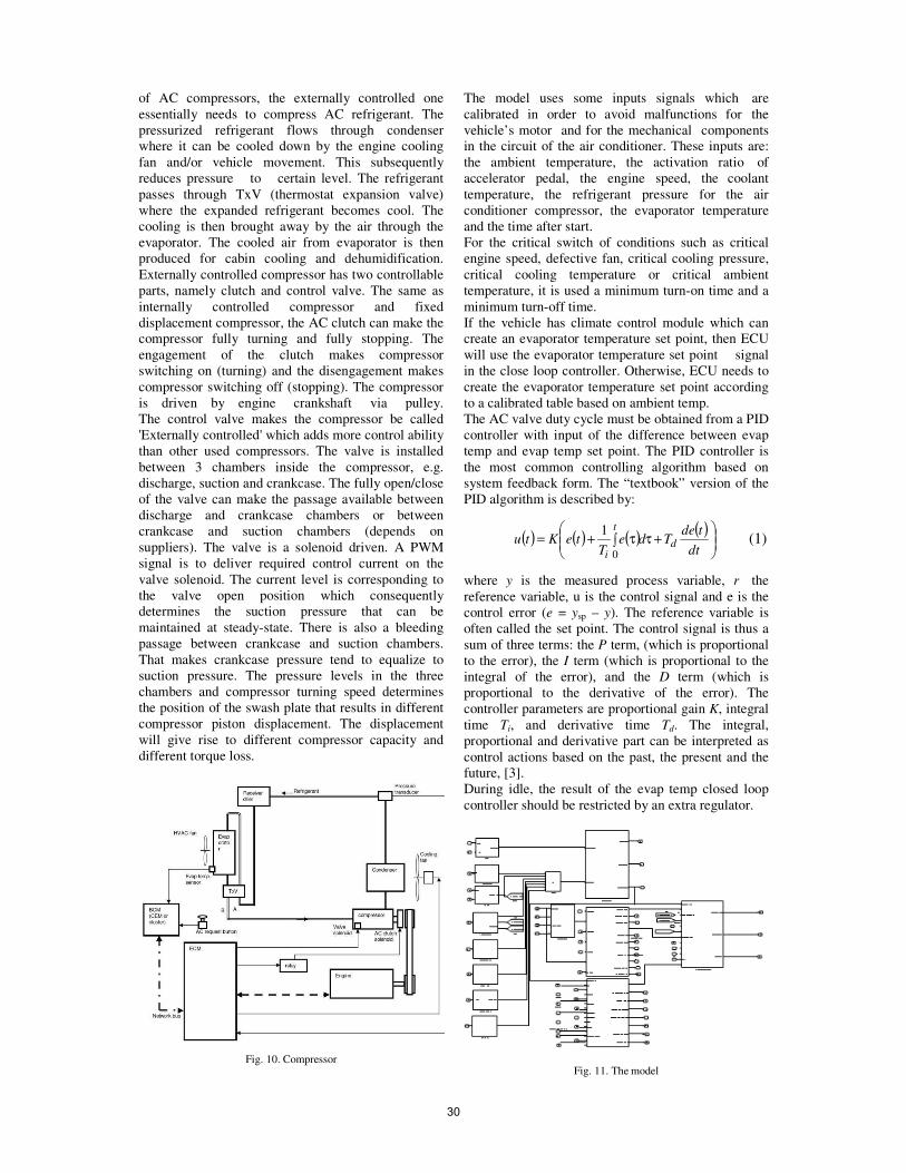
of AC compressors, the externally controlled one
essentially needs to compress AC refrigerant. The
pressurized refrigerant flows through condenser
where it can be cooled down by the engine cooling
fan and/or vehicle movement. This subsequently
reduces pressure to certain level. The refrigerant
passes through TxV (thermostat expansion valve)
where the expanded refrigerant becomes cool. The
cooling is then brought away by the air through the
evaporator. The cooled air from evaporator is then
produced for cabin cooling and dehumidification.
Externally controlled compressor has two controllable
parts, namely clutch and control valve. The same as
internally controlled compressor and fixed
displacement compressor, the AC clutch can make the
compressor fully turning and fully stopping. The
engagement of the clutch makes compressor
switching on (turning) and the disengagement makes
compressor switching off (stopping). The compressor
is driven by engine crankshaft via pulley.
The control valve makes the compressor be called
'Externally controlled' which adds more control ability
than other used compressors. The valve is installed
between 3 chambers inside the compressor, e.g.
discharge, suction and crankcase. The fully open/close
of the valve can make the passage available between
discharge and crankcase chambers or between
crankcase and suction chambers (depends on
suppliers). The valve is a solenoid driven. A PWM
signal is to deliver required control current on the
valve solenoid. The current level is corresponding to
the valve open position which consequently
determines the suction pressure that can be
maintained at steady-state. There is also a bleeding
passage between crankcase and suction chambers.
That makes crankcase pressure tend to equalize to
suction pressure. The pressure levels in the three
chambers and compressor turning speed determines
the position of the swash plate that results in different
compressor piston displacement. The displacement
will give rise to different compressor capacity and
different torque loss.
Fig. 10. Compressor
The model uses some inputs signals which are
calibrated in order to avoid malfunctions for the
vehicle’s motor and for the mechanical components
in the circuit of the air conditioner. These inputs are:
the ambient temperature, the activation ratio of
accelerator pedal, the engine speed, the coolant
temperature, the refrigerant pressure for the air
conditioner compressor, the evaporator temperature
and the time after start.
For the critical switch of conditions such as critical
engine speed, defective fan, critical cooling pressure,
critical cooling temperature or critical ambient
temperature, it is used a minimum turn-on time and a
minimum turn-off time.
If the vehicle has climate control module which can
create an evaporator temperature set point, then ECU
will use the evaporator temperature set point signal
in the close loop controller. Otherwise, ECU needs to
create the evaporator temperature set point according
to a calibrated table based on ambient temp.
The AC valve duty cycle must be obtained from a PID
controller with input of the difference between evap
temp and evap temp set point. The PID controller is
the most common controlling algorithm based on
system feedback form. The “textbook” version of the
PID algorithm is described by:
( ) ( ) ( )( )
+τ∫ τ+=
dt
tdeTde
TteKtu d
t
i 0
1 (1)
where y is the measured process variable, r the
reference variable, u is the control signal and e is the
control error (e = ysp – y). The reference variable is
often called the set point. The control signal is thus a
sum of three terms: the P term, (which is proportional
to the error), the I term (which is proportional to the
integral of the error), and the D term (which is
proportional to the derivative of the error). The
controller parameters are proportional gain K, integral
time Ti, and derivative time Td. The integral,
proportional and derivative part can be interpreted as
control actions based on the past, the present and the
future, [3].
During idle, the result of the evap temp closed loop
controller should be restricted by an extra regulator.
Fig. 11. The model
30

If demanded torque is smaller than a lower threshold,
then the duty cycle obtained from the evap temp
closed loop controller should be directly used. The
lower threshold is the product of max available torque
and a calibrated factor.
If demanded torque is greater than an upper threshold,
then a valve duty cycle increment should be used. The
increment is obtained from a calibrated table as a
function maximum available torque. The upper
threshold is the product of max available torque and
another calibrated factor.
If engine is in launch operation, then the AC
compressor should work at a degraded condition or
disengage AC clutch. At transition of A/C clutch
engagement to disengagement due to launch cut-out,
initialized cut-out timer starts decrementing.
If there is any request to minimize the AC valve duty
cycle for any function, then the valve duty cycle
should be firstly minimized to a calibrated level. If
AC clutch is disengaged for AC off request, then the
valve duty cycle should also be minimized.
The model will be then compiled and for
optimization, the model was simulated with a single
step, discret, and with the ode 5 solver. After the
simulation there were generated o series of files with
different extensions, from them de .sdf file was used.
First part of the experiment in ControlDesk is to
create a project for which the .sdf file from the
Simulink model, will be used. For visualization and
controlling the desired parameters the a .lay file will
be used, after this we can use different instrument like
controllers, indicators, plotters etc. In figure 12, we
have a GUI made in the ControlDesk, the interface
presents the inhibitions from the model in Simulink,
respectively the ambient temperature, the activation
ratio of accelerator pedal, the engine speed, the
coolant temperature, the refrigerant pressure for the
air conditioner compressor, the evaporator
temperature and the time after start.
In the last part of the experiment, the PWM signal
from the model is present on one pin from the
Fig. 12. The GUI from ControlDesk
Fig. 13. The PWM signal on the osciloscope
DS2201 board on the AutoBox. The signal can be
seen on the oscilloscope, as shown in figure 13. In
order to see the signal on the DS2201 board we have
to use the dSPACE RTI1005 library in the Simulink
model. This library consits of : I/O units for ADC,
DAC convertors, digital I/O, signal generation and
frequency measurements. Real-Time Interface (RTI)
is the link between dSPACE hardware and the
development software MATLAB/Simulink/Stateflow
from The MathWorks, [7].
VI. CONCLUSION
The model was developed for the control of the
vehicle’s air conditioner compressor using a PWM
signal. The AutoBox from dSPACE together with the
ControlDesk helps us represent the signal in Real
Time.
REFERENCES
[1] Air Conditioner in the Motor Vehicle, Self-Study Programme
208
[2] Getting Started Guide - Simulink, Matlab & Simulink,
MathWorks, 2014
[3] Karl Johan Åström, Control System Design, Lecture Notes for
ME 155A, Santa Barbara, 2000 [4] Simulink. Simulation and Model-Based Design, MathWorks,
2014
[5]http://www.dspace.com/en/pub/home/products/hw/accessories/a
utobox.cfm
[6] Hardware Installation and Configuration Refrence, Modular
Systems, dSPACE
[7] Real Time Interface from dSPACE
31

Buletinul Ştiinţific al Universităţii Timişoara
TRANSACTIONS on ELECTRONICS and COMMUNICATIONS
Volume 59(73), Issue 2, 2014
Instructions for authors at the Scientific Bulletin of the
Politehnica University of Timisoara - Transactions on
Electronics and Communications
First Author1 Second Author
2
1 Faculty of Electronics and Telecommunications, Communications Dept. Bd. V. Parvan 2, 300223 Timisoara, Romania, e-mail [email protected] 2 Faculty of Electronics and Telecommunications, Communications Dept.
Bd. V. Parvan 2, 300223 Timisoara, Romania, e-mail [email protected]
Abstract – These instructions present a model for editing
the papers accepted at the Scientific Bulletin of
“Politehnica” University of Timisoara, Transactions on
Electronics and Communications. The abstract should
contain the description of the problem, methods,
solutions and results in a maximum of 12 lines. No
references are allowed here.
Keywords: editing, Bulletin, author
I. INTRODUCTION
The page format is A4. The articles must be of 6
pages or less, tables and figures included.
II. GUIDELINES
The paper should be sent in this standard form. Use a
good quality printer, and print on a single face of the
sheet. Use a double column format with 0.5 cm in
between columns, on an A4, portrait oriented,
standard size. The top and bottom margins should be
of 2.28 cm, and the left and right margins of 2.54 cm.
Microsoft Word for Windows is recommended as a
text editor. Choose Times New Roman fonts, and
single spaced lines. Font sizes should be: 18 pt bold
for the paper title, 12 pt for the author(s), 9 pt bold for
the abstract and keywords, 10 pt capitals for the
section titles, 10 pt italic for the subsection titles;
distance between section numbers and titles should be
of 0.25 cm; use 10 pt for the normal text, 8 pt for
affiliation, footnotes, figure captions, and references.
III. FIGURES AND TABLES
Figures should be centered, and tables should be left
aligned, and should be placed after the first reference
in the text. Use abbreviations such as “Fig.1.” even at
the beginning of the sentence. Leave an empty line
before and after equations. Equation numbering
should be simple: (1), (2), (3) … and right aligned:
∫−
−=
a
adtytx ττ )()( . (1)
IV. ABOUT REFERENCES
References should be numbered in a simple form [1],
[2], [3]…, and quoted accordingly [1]. References are
not allowed in footnotes. It is recommended to
mention all authors; “et al.” should be used only for
more than 6 authors.
Table 1
Parameter Value Unit
I 2.4 A
U 10.0 V
V. REMARKS
A. Abbreviations and acronyms
Abbreviations and acronyms should be explained
when they appear for the first time in the text.
Abbreviations such as IEEE, IEE, SI, MKS, CGS, ac,
dc and rms need no further explanation. It is
recommended not to use abbreviations in section or
subsection titles.
Fig. 1. Amplitudes in the standing wave
32

B. Further recommendations
The International System of units is recommended.
Do not mix SI and CGS. Preliminary, experimental
results are not accepted. Roman section numbering is
optional.
REFERENCES
[1] A. Ignea, “Preparation of papers for the International
Symposium Etc. ’98”, Buletinul Universităţii “Politehnica”, Seria
Electrotehnica, Electronica si Telecomunicatii, Tom 43 (57), 1998,
Fascicola 1, 1998, pp. 81.
[2] R. E. Collin, Foundations for Microwave Engineering, Second
Edition, McGraw-Hill, Inc., 1992.
[3] http://www.tc.etc.upt.ro/bulletin
33