edited by Olivier Chapelle, Bernhard Schölkopf, and Alexander … SemiSupervised Lear… · ·...
524
Semi-Supervised Learning edited by Olivier Chapelle, Bernhard Schölkopf, and Alexander Zien
-
Upload
nguyentruc -
Category
Documents
-
view
217 -
download
2
Transcript of edited by Olivier Chapelle, Bernhard Schölkopf, and Alexander … SemiSupervised Lear… · ·...

Semi-Supervised Learning
edited by
Olivier Chapelle,
Bernhard Schölkopf,
and Alexander Zien

Semi-Supervised Learning

Adaptive Computation and Machine Learning
Thomas Dietterich, Editor
Christopher Bishop, David Heckerman, Michael Jordan, and Michael Kearns, As-
sociate Editors
Bioinformatics: The Machine Learning Approach, Pierre Baldi and Søren Brunak
Reinforcement Learning: An Introduction, Richard S. Sutton and Andrew G. Barto
Graphical Models for Machine Learning and Digital Communication, Brendan J.
Frey
Learning in Graphical Models, Michael I. Jordan
Causation, Prediction, and Search, second edition, Peter Spirtes, Clark Glymour,
and Richard Scheines
Principles of Data Mining, David Hand, Heikki Mannila, and Padhraic Smyth
Bioinformatics: The Machine Learning Approach, second edition, Pierre Baldi and
Søren Brunak
Learning Kernel Classifiers: Theory and Algorithms, Ralf Herbrich
Learning with Kernels: Support Vector Machines, Regularization, Optimization, and
Beyond, Bernhard Scholkopf and Alexander J. Smola
Introduction to Machine Learning, Ethem Alpaydin
Gaussian Processes for Machine Learning, Carl Edward Rasmussen and Christo-
pher K. I. Williams
Semi-Supervised Learning, Olivier Chapelle, Bernhard Scholkopf, and Alexander
Zien

Semi-Supervised Learning
Olivier Chapelle
Bernhard Scholkopf
Alexander Zien
The MIT Press
Cambridge, Massachusetts
London, England

c©2006 Massachusetts Institute of Technology
All rights reserved. No part of this book may be reproduced in any form by any electronic
or mechanical means (including photocopying, recording, or information storage and retrieval)
without permission in writing from the publisher.
Typeset by the authors using LATEX2ε
Printed and bound in the United States of America
Library of Congress Cataloging-in-Publication Data
Semi-supervised learning / edited by Olivier Chapelle, Bernhard Scholkopf, Alexander Zien.
p. cm. – (Adaptive computation and machine learning)
Includes bibliographical references.
ISBN 978-0-262-03358-9 (alk. paper)
1. Supervised learning (Machine learning) I. Chapelle, Olivier. II. Scholkopf, Bernhard. III. Zien,
Alexander. IV. Series.
Q325.75.S42 2006 006.3’1–dc22 2006044448
10 9 8 7 6 5 4 3 2 1

Contents
Series Foreword xi
Preface xiii
1 Introduction to Semi-Supervised Learning 1
1.1 Supervised, Unsupervised, and Semi-Supervised Learning . . . . . . 1
1.2 When Can Semi-Supervised Learning Work? . . . . . . . . . . . . . 4
1.3 Classes of Algorithms and Organization of This Book . . . . . . . . 8
I Generative Models 13
2 A Taxonomy for Semi-Supervised Learning Methods 15
Matthias Seeger
2.1 The Semi-Supervised Learning Problem . . . . . . . . . . . . . . . . 15
2.2 Paradigms for Semi-Supervised Learning . . . . . . . . . . . . . . . . 17
2.3 Examples . . . . . . . . . . . . . . . . . . . . . . . . . . . . . . . . . 22
2.4 Conclusions . . . . . . . . . . . . . . . . . . . . . . . . . . . . . . . . 31
3 Semi-Supervised Text Classification Using EM 33
Kamal Nigam, Andrew McCallum, Tom Mitchell
3.1 Introduction . . . . . . . . . . . . . . . . . . . . . . . . . . . . . . . . 33
3.2 A Generative Model for Text . . . . . . . . . . . . . . . . . . . . . . 35
3.3 Experimental Results with Basic EM . . . . . . . . . . . . . . . . . . 41
3.4 Using a More Expressive Generative Model . . . . . . . . . . . . . . 43
3.5 Overcoming the Challenges of Local Maxima . . . . . . . . . . . . . 49
3.6 Conclusions and Summary . . . . . . . . . . . . . . . . . . . . . . . . 54
4 Risks of Semi-Supervised Learning 57
Fabio Cozman, Ira Cohen
4.1 Do Unlabeled Data Improve or Degrade Classification Performance? 57
4.2 Understanding Unlabeled Data: Asymptotic Bias . . . . . . . . . . . 59
4.3 The Asymptotic Analysis of Generative Semi-Supervised Learning . 63
4.4 The Value of Labeled and Unlabeled Data . . . . . . . . . . . . . . . 67
4.5 Finite Sample Effects . . . . . . . . . . . . . . . . . . . . . . . . . . . 69

vi Contents
4.6 Model Search and Robustness . . . . . . . . . . . . . . . . . . . . . . 70
4.7 Conclusion . . . . . . . . . . . . . . . . . . . . . . . . . . . . . . . . 71
5 Probabilistic Semi-Supervised Clustering with Constraints 73
Sugato Basu, Mikhail Bilenko, Arindam Banerjee, Raymond Mooney
5.1 Introduction . . . . . . . . . . . . . . . . . . . . . . . . . . . . . . . . 74
5.2 HMRF Model for Semi-Supervised Clustering . . . . . . . . . . . . . 75
5.3 HMRF-KMeans Algorithm . . . . . . . . . . . . . . . . . . . . . . 81
5.4 Active Learning for Constraint Acquisition . . . . . . . . . . . . . . 93
5.5 Experimental Results . . . . . . . . . . . . . . . . . . . . . . . . . . . 96
5.6 Related Work . . . . . . . . . . . . . . . . . . . . . . . . . . . . . . . 100
5.7 Conclusions . . . . . . . . . . . . . . . . . . . . . . . . . . . . . . . . 101
II Low-Density Separation 103
6 Transductive Support Vector Machines 105
Thorsten Joachims
6.1 Introduction . . . . . . . . . . . . . . . . . . . . . . . . . . . . . . . . 105
6.2 Transductive Support Vector Machines . . . . . . . . . . . . . . . . . 108
6.3 Why Use Margin on the Test Set? . . . . . . . . . . . . . . . . . . . 111
6.4 Experiments and Applications of TSVMs . . . . . . . . . . . . . . . 112
6.5 Solving the TSVM Optimization Problem . . . . . . . . . . . . . . . 114
6.6 Connection to Related Approaches . . . . . . . . . . . . . . . . . . . 116
6.7 Summary and Conclusions . . . . . . . . . . . . . . . . . . . . . . . . 116
7 Semi-Supervised Learning Using Semi-Definite Programming 119
Tijl De Bie, Nello Cristianini
7.1 Relaxing SVM Transduction . . . . . . . . . . . . . . . . . . . . . . . 119
7.2 An Approximation for Speedup . . . . . . . . . . . . . . . . . . . . . 126
7.3 General Semi-Supervised Learning Settings . . . . . . . . . . . . . . 128
7.4 Empirical Results . . . . . . . . . . . . . . . . . . . . . . . . . . . . . 129
7.5 Summary and Outlook . . . . . . . . . . . . . . . . . . . . . . . . . . 133
Appendix: The Extended Schur Complement Lemma . . . . . . . . . 134
8 Gaussian Processes and the Null-Category Noise Model 137
Neil D. Lawrence, Michael I. Jordan
8.1 Introduction . . . . . . . . . . . . . . . . . . . . . . . . . . . . . . . . 137
8.2 The Noise Model . . . . . . . . . . . . . . . . . . . . . . . . . . . . . 141
8.3 Process Model and Effect of the Null-Category . . . . . . . . . . . . 143
8.4 Posterior Inference and Prediction . . . . . . . . . . . . . . . . . . . 145
8.5 Results . . . . . . . . . . . . . . . . . . . . . . . . . . . . . . . . . . . 147
8.6 Discussion . . . . . . . . . . . . . . . . . . . . . . . . . . . . . . . . . 149
9 Entropy Regularization 151

Contents vii
Yves Grandvalet, Yoshua Bengio
9.1 Introduction . . . . . . . . . . . . . . . . . . . . . . . . . . . . . . . . 151
9.2 Derivation of the Criterion . . . . . . . . . . . . . . . . . . . . . . . . 152
9.3 Optimization Algorithms . . . . . . . . . . . . . . . . . . . . . . . . 155
9.4 Related Methods . . . . . . . . . . . . . . . . . . . . . . . . . . . . . 158
9.5 Experiments . . . . . . . . . . . . . . . . . . . . . . . . . . . . . . . . 160
9.6 Conclusion . . . . . . . . . . . . . . . . . . . . . . . . . . . . . . . . 166
Appendix: Proof of Theorem 9.1 . . . . . . . . . . . . . . . . . . . . 166
10 Data-Dependent Regularization 169
Adrian Corduneanu, Tommi Jaakkola
10.1 Introduction . . . . . . . . . . . . . . . . . . . . . . . . . . . . . . . . 169
10.2 Information Regularization on Metric Spaces . . . . . . . . . . . . . 174
10.3 Information Regularization and Relational Data . . . . . . . . . . . . 182
10.4 Discussion . . . . . . . . . . . . . . . . . . . . . . . . . . . . . . . . . 189
III Graph-Based Methods 191
11 Label Propagation and Quadratic Criterion 193
Yoshua Bengio, Olivier Delalleau, Nicolas Le Roux
11.1 Introduction . . . . . . . . . . . . . . . . . . . . . . . . . . . . . . . . 193
11.2 Label Propagation on a Similarity Graph . . . . . . . . . . . . . . . 194
11.3 Quadratic Cost Criterion . . . . . . . . . . . . . . . . . . . . . . . . 198
11.4 From Transduction to Induction . . . . . . . . . . . . . . . . . . . . 205
11.5 Incorporating Class Prior Knowledge . . . . . . . . . . . . . . . . . . 205
11.6 Curse of Dimensionality for Semi-Supervised Learning . . . . . . . . 206
11.7 Discussion . . . . . . . . . . . . . . . . . . . . . . . . . . . . . . . . . 215
12 The Geometric Basis of Semi-Supervised Learning 217
Vikas Sindhwani, Misha Belkin, Partha Niyogi
12.1 Introduction . . . . . . . . . . . . . . . . . . . . . . . . . . . . . . . . 217
12.2 Incorporating Geometry in Regularization . . . . . . . . . . . . . . . 220
12.3 Algorithms . . . . . . . . . . . . . . . . . . . . . . . . . . . . . . . . 224
12.4 Data-Dependent Kernels for Semi-Supervised Learning . . . . . . . . 229
12.5 Linear Methods for Large-Scale Semi-Supervised Learning . . . . . . 231
12.6 Connections to Other Algorithms and Related Work . . . . . . . . . 232
12.7 Future Directions . . . . . . . . . . . . . . . . . . . . . . . . . . . . . 234
13 Discrete Regularization 237
Dengyong Zhou, Bernhard Scholkopf
13.1 Introduction . . . . . . . . . . . . . . . . . . . . . . . . . . . . . . . . 237
13.2 Discrete Analysis . . . . . . . . . . . . . . . . . . . . . . . . . . . . . 239
13.3 Discrete Regularization . . . . . . . . . . . . . . . . . . . . . . . . . 245
13.4 Conclusion . . . . . . . . . . . . . . . . . . . . . . . . . . . . . . . . 249

viii Contents
14 Semi-Supervised Learning with Conditional Harmonic Mixing 251
Christopher J. C. Burges, John C. Platt
14.1 Introduction . . . . . . . . . . . . . . . . . . . . . . . . . . . . . . . . 251
14.2 Conditional Harmonic Mixing . . . . . . . . . . . . . . . . . . . . . . 255
14.3 Learning in CHM Models . . . . . . . . . . . . . . . . . . . . . . . . 256
14.4 Incorporating Prior Knowledge . . . . . . . . . . . . . . . . . . . . . 261
14.5 Learning the Conditionals . . . . . . . . . . . . . . . . . . . . . . . . 261
14.6 Model Averaging . . . . . . . . . . . . . . . . . . . . . . . . . . . . . 262
14.7 Experiments . . . . . . . . . . . . . . . . . . . . . . . . . . . . . . . . 263
14.8 Conclusions . . . . . . . . . . . . . . . . . . . . . . . . . . . . . . . . 273
IV Change of Representation 275
15 Graph Kernels by Spectral Transforms 277
Xiaojin Zhu, Jaz Kandola, John Lafferty, Zoubin Ghahramani
15.1 The Graph Laplacian . . . . . . . . . . . . . . . . . . . . . . . . . . . 278
15.2 Kernels by Spectral Transforms . . . . . . . . . . . . . . . . . . . . . 280
15.3 Kernel Alignment . . . . . . . . . . . . . . . . . . . . . . . . . . . . . 281
15.4 Optimizing Alignment Using QCQP for Semi-Supervised Learning . 282
15.5 Semi-Supervised Kernels with Order Constraints . . . . . . . . . . . 283
15.6 Experimental Results . . . . . . . . . . . . . . . . . . . . . . . . . . . 285
15.7 Conclusion . . . . . . . . . . . . . . . . . . . . . . . . . . . . . . . . 289
16 Spectral Methods for Dimensionality
Reduction 293
Lawrence K. Saul, Kilian Q. Weinberger, Fei Sha, Jihun Ham, Daniel D. Lee
16.1 Introduction . . . . . . . . . . . . . . . . . . . . . . . . . . . . . . . . 293
16.2 Linear Methods . . . . . . . . . . . . . . . . . . . . . . . . . . . . . . 295
16.3 Graph-Based Methods . . . . . . . . . . . . . . . . . . . . . . . . . . 297
16.4 Kernel Methods . . . . . . . . . . . . . . . . . . . . . . . . . . . . . . 303
16.5 Discussion . . . . . . . . . . . . . . . . . . . . . . . . . . . . . . . . . 306
17 Modifying Distances 309
Sajama, Alon Orlitsky
17.1 Introduction . . . . . . . . . . . . . . . . . . . . . . . . . . . . . . . . 309
17.2 Estimating DBD Metrics . . . . . . . . . . . . . . . . . . . . . . . . . 312
17.3 Computing DBD Metrics . . . . . . . . . . . . . . . . . . . . . . . . 321
17.4 Semi-Supervised Learning Using Density-Based Metrics . . . . . . . 327
17.5 Conclusions and Future Work . . . . . . . . . . . . . . . . . . . . . . 329
V Semi-Supervised Learning in Practice 331
18 Large-Scale Algorithms 333

Contents ix
Olivier Delalleau, Yoshua Bengio, Nicolas Le Roux
18.1 Introduction . . . . . . . . . . . . . . . . . . . . . . . . . . . . . . . . 333
18.2 Cost Approximations . . . . . . . . . . . . . . . . . . . . . . . . . . . 334
18.3 Subset Selection . . . . . . . . . . . . . . . . . . . . . . . . . . . . . 337
18.4 Discussion . . . . . . . . . . . . . . . . . . . . . . . . . . . . . . . . . 340
19 Semi-Supervised Protein Classification
Using Cluster Kernels 343
Jason Weston, Christina Leslie, Eugene Ie, William Stafford Noble
19.1 Introduction . . . . . . . . . . . . . . . . . . . . . . . . . . . . . . . . 343
19.2 Representations and Kernels for Protein Sequences . . . . . . . . . . 345
19.3 Semi-Supervised Kernels for Protein Sequences . . . . . . . . . . . . 348
19.4 Experiments . . . . . . . . . . . . . . . . . . . . . . . . . . . . . . . . 352
19.5 Discussion . . . . . . . . . . . . . . . . . . . . . . . . . . . . . . . . . 358
20 Prediction of Protein Function from
Networks 361
Hyunjung Shin, Koji Tsuda
20.1 Introduction . . . . . . . . . . . . . . . . . . . . . . . . . . . . . . . . 361
20.2 Graph-Based Semi-Supervised Learning . . . . . . . . . . . . . . . . 364
20.3 Combining Multiple Graphs . . . . . . . . . . . . . . . . . . . . . . . 366
20.4 Experiments on Function Prediction of Proteins . . . . . . . . . . . . 369
20.5 Conclusion and Outlook . . . . . . . . . . . . . . . . . . . . . . . . . 374
21 Analysis of Benchmarks 377
21.1 The Benchmark . . . . . . . . . . . . . . . . . . . . . . . . . . . . . . 377
21.2 Application of SSL Methods . . . . . . . . . . . . . . . . . . . . . . . 383
21.3 Results and Discussion . . . . . . . . . . . . . . . . . . . . . . . . . . 390
VI Perspectives 395
22 An Augmented PAC Model for Semi-Supervised Learning 397
Maria-Florina Balcan, Avrim Blum
22.1 Introduction . . . . . . . . . . . . . . . . . . . . . . . . . . . . . . . . 398
22.2 A Formal Framework . . . . . . . . . . . . . . . . . . . . . . . . . . . 400
22.3 Sample Complexity Results . . . . . . . . . . . . . . . . . . . . . . . 403
22.4 Algorithmic Results . . . . . . . . . . . . . . . . . . . . . . . . . . . 412
22.5 Related Models and Discussion . . . . . . . . . . . . . . . . . . . . . 416
23 Metric-Based Approaches for Semi-
Supervised Regression and Classification 421
Dale Schuurmans, Finnegan Southey, Dana Wilkinson, Yuhong Guo
23.1 Introduction . . . . . . . . . . . . . . . . . . . . . . . . . . . . . . . . 421
23.2 Metric Structure of Supervised Learning . . . . . . . . . . . . . . . . 423

x Contents
23.3 Model Selection . . . . . . . . . . . . . . . . . . . . . . . . . . . . . . 426
23.4 Regularization . . . . . . . . . . . . . . . . . . . . . . . . . . . . . . 436
23.5 Classification . . . . . . . . . . . . . . . . . . . . . . . . . . . . . . . 445
23.6 Conclusion . . . . . . . . . . . . . . . . . . . . . . . . . . . . . . . . 449
24 Transductive Inference and
Semi-Supervised Learning 453
Vladimir Vapnik
24.1 Problem Settings . . . . . . . . . . . . . . . . . . . . . . . . . . . . . 453
24.2 Problem of Generalization in Inductive and Transductive Inference . 455
24.3 Structure of the VC Bounds and Transductive Inference . . . . . . . 457
24.4 The Symmetrization Lemma and Transductive Inference . . . . . . . 458
24.5 Bounds for Transductive Inference . . . . . . . . . . . . . . . . . . . 459
24.6 The Structural Risk Minimization Principle for Induction and Trans-
duction . . . . . . . . . . . . . . . . . . . . . . . . . . . . . . . . . . 460
24.7 Combinatorics in Transductive Inference . . . . . . . . . . . . . . . . 462
24.8 Measures of the Size of Equivalence Classes . . . . . . . . . . . . . . 463
24.9 Algorithms for Inductive and Transductive SVMs . . . . . . . . . . . 465
24.10 Semi-Supervised Learning . . . . . . . . . . . . . . . . . . . . . . . 470
24.11 Conclusion: Transductive Inference and the New Problems of Infer-
ence . . . . . . . . . . . . . . . . . . . . . . . . . . . . . . . . . . . . 470
24.12 Beyond Transduction: Selective Inference . . . . . . . . . . . . . . . 471
25 A Discussion of Semi-Supervised Learning and Transduction 473
References 479
Notation and Symbols 499
Contributors 503
Index 509

Series Foreword
The goal of building systems that can adapt to their environments and learn from
their experience has attracted researchers from many fields, including computer
science, engineering, mathematics, physics, neuroscience, and cognitive science.
Out of this research has come a wide variety of learning techniques that have
the potential to transform many scientific and industrial fields. Recently, several
research communities have converged on a common set of issues surrounding su-
pervised, unsupervised, and reinforcement learning problems. The MIT Press series
on Adaptive Computation and Machine Learning seeks to unify the many diverse
strands of machine learning research and to foster high-quality research and inno-
vative applications.
Thomas Dietterich


Preface
During the last years, semi-supervised learning has emerged as an exciting new
direction in machine learning reseach. It is closely related to profound issues of how
to do inference from data, as witnessed by its overlap with transductive inference
(the distinctions are yet to be made precise).
At the same time, dealing with the situation where relatively few labeled training
points are available, but a large number of unlabeled points are given, it is directly
relevant to a multitude of practical problems where is it relatively expensive to
produce labeled data, e.g., the automatic classification of web pages. As a field,
semi-supervised learning uses a diverse set of tools and illustrates, on a small scale,
the sophisticated machinery developed in various branches of machine learning such
as kernel methods or Bayesian techniques.
As we work on semi-supervised learning, we have been aware of the lack of
an authoritative overview of the existing approaches. In a perfect world, such an
overview should help both the practitioner and the researcher who wants to enter
this area. A well researched monograph could ideally fill such a gap; however, the
field of semi-supervised learning is arguably not yet sufficiently mature for this.
Rather than writing a book which would come out in three years, we thus decided
instead to provide an up-to-date edited volume, where we invited contributions by
many of the leading proponents of the field. To make it more than a mere collection
of articles, we have attempted to ensure that the chapters form a coherent whole
and use consistent notation. Moreover, we have written a short introduction, a
dialogue illustrating some of the ongoing debates in the underlying philosophy of
the field, and we have organized and summarized a comprehensive benchmark of
semi-supervised learning.
Benchmarks are helpful for the practitioner to decide which algorithm should be
chosen for a given application. At the same time, they are useful for researchers
to choose issues to study and further develop. By evaluating and comparing the
performance of many of the presented methods on a set of eight benchmark
problems, this book aims at providing guidance in this respect. The problems are
designed to reflect and probe the different assumptions that the algorithms build
on. All data sets can be downloaded from the book web page, which can be found
at http://www.kyb.tuebingen.mpg.de/ssl-book/.
Finally, we would like to give thanks to everybody who contributed towards the
success of this book project, in particular to Karin Bierig, Sabrina Nielebock, Bob
Prior, to all chapter authors, and to the chapter reviewers.


1 Introduction to Semi-Supervised Learning
1.1 Supervised, Unsupervised, and Semi-Supervised Learning
In order to understand the nature of semi-supervised learning, it will be useful first
to take a look at supervised and unsupervised learning.
1.1.1 Supervised and Unsupervised Learning
Traditionally, there have been two fundamentally different types of tasks in machine
learning.
The first one is unsupervised learning. Let X = (x1, . . . , xn) be a set of n examplesunsupervised
learning (or points), where xi ∈ X for all i ∈ [n] := 1, . . . , n. Typically it is assumed
that the points are drawn i.i.d. (independently and identically distributed) from
a common distribution on X. It is often convenient to define the (n × d)-matrix
X = (x⊤i )⊤i∈[n] that contains the data points as its rows. The goal of unsupervised
learning is to find interesting structure in the data X . It has been argued that the
problem of unsupervised learning is fundamentally that of estimating a density
which is likely to have generated X . However, there are also weaker forms of
unsupervised learning, such as quantile estimation, clustering, outlier detection,
and dimensionality reduction.
The second task is supervised learning. The goal is to learn a mapping fromsupervised
learning x to y, given a training set made of pairs (xi, yi). Here, the yi ∈ Y are called
the labels or targets of the examples xi. If the labels are numbers, y = (yi)⊤i∈[n]
denotes the column vector of labels. Again, a standard requirement is that the pairs
(xi, yi) are sampled i.i.d. from some distribution which here ranges over X × Y.
The task is well defined, since a mapping can be evaluated through its predictive
performance on test examples. When Y = R or Y = Rd (or more generally, when the
labels are continuous), the task is called regression. Most of this book will focus on
classification (there is some work on regression in chapter 23), i.e., the case where
y takes values in a finite set (discrete labels). There are two families of algorithms
for supervised learning. Generative algorithms try to model the class-conditionalgenerative
methods

2 Introduction to Semi-Supervised Learning
density p(x|y) by some unsupervised learning procedure.1 A predictive density can
then be inferred by applying Bayes theorem:
p(y|x) =p(x|y)p(y)∫
Yp(x|y)p(y)dy
. (1.1)
In fact, p(x|y)p(y) = p(x, y) is the joint density of the data, from which pairs
(xi, yi) could be generated. Discriminative algorithms do not try to estimate howdiscriminative
methods the xi have been generated, but instead concentrate on estimating p(y|x). Some
discriminative methods even limit themselves to modeling whether p(y|x) is greater
than or less than 0.5; an example of this is the support vector machine (SVM). It
has been argued that discriminative models are more directly aligned with the goal
of supervised learning and therefore tend to be more efficient in practice. These two
frameworks are discussed in more detail in sections 2.2.1 and 2.2.2.
1.1.2 Semi-Supervised Learning
Semi-supervised learning (SSL) is halfway between supervised and unsupervised
learning. In addition to unlabeled data, the algorithm is provided with some super-
vision information – but not necessarily for all examples. Often, this information
will be the targets associated with some of the examples. In this case, the datastandard setting
of SSL set X = (xi)i∈[n] can be divided into two parts: the points Xl := (x1, . . . , xl), for
which labels Yl := (y1, . . . , yl) are provided, and the points Xu := (xl+1, . . . , xl+u),
the labels of which are not known. This is “standard” semi-supervised learning as
investigated in this book; most chapters will refer to this setting.
Other forms of partial supervision are possible. For example, there may be
constraints such as “these points have (or do not have) the same target” (cf.
Abu-Mostafa, 1995). This more general setting is considered in chapter 5. TheSSL with
constraints different setting corresponds to a different view of semi-supervised learning: In
chapter 5, SSL is seen as unsupervised learning guided by constraints. In contrast,
most other approaches see SSL as supervised learning with additional information
on the distribution of the examples x. The latter interpretation seems to be more
in line with most applications, where the goal is the same as in supervised learning:
to predict a target value for a given xi. However, this view does not readily apply
if the number and nature of the classes are not known in advance but have to be
inferred from the data. In constrast, SSL as unsupervised learning with constraints
may still remain applicable in such situations.
A problem related to SSL was introduced by Vapnik already several decades ago:
so-called transductive learning. In this setting, one is given a (labeled) training settransductive
learning and an (unlabeled) test set. The idea of transduction is to perform predictions only
for the test points. This is in contrast to inductive learning, where the goal is toinductive learning
1. For simplicity, we are assuming that all distributions have densities, and thus we restrictourselves to dealing with densities.

1.1 Supervised, Unsupervised, and Semi-Supervised Learning 3
output a prediction function which is defined on the entire space X. Many methods
described in this book will be transductive; in particular, this is rather natural for
inference based on graph representations of the data. This issue will be addressed
again in section 1.2.4.
1.1.3 A Brief History of Semi-Supervised Learning
Probably the earliest idea about using unlabeled data in classification is self-
learning, which is also known as self-training, self-labeling, or decision-directedself-learning
learning. This is a wrapper-algorithm that repeatedly uses a supervised learning
method. It starts by training on the labeled data only. In each step a part of
the unlabeled points is labeled according to the current decision function; then
the supervised method is retrained using its own predictions as additional labeled
points. This idea has appeared in the literature already for some time (e.g., Scudder
(1965); Fralick (1967); Agrawala (1970)).
An unsatisfactory aspect of self-learning is that the effect of the wrapper depends
on the supervised method used inside it. If self-learning is used with empirical risk
minimization and 1-0-loss, the unlabeled data will have no effect on the solution
at all. If instead a margin maximizing method is used, as a result the decision
boundary is pushed away from the unlabeled points (cf. chapter 6). In other cases
it seems to be unclear what the self-learning is really doing, and which assumption
it corresponds to.
Closely related to semi-supervised learning is the concept of transductive
inference, or transduction, pioneered by Vapnik (Vapnik and Chervonenkis, 1974;transductive
inference Vapnik and Sterin, 1977). In contrast to inductive inference, no general decision rule
is inferred, but only the labels of the unlabeled (or test) points are predicted. An
early instance of transduction (albeit without explicitly considering it as a concept)
was already proposed by Hartley and Rao (1968). They suggested a combinatorial
optimization on the labels of the test points in order to maximize the likelihood of
their model.
It seems that semi-supervised learning really took off in the 1970s when the
problem of estimating the Fisher linear discriminant rule with unlabeled datamixture of
Gaussians was considered (Hosmer, 1973; McLachlan, 1977; O’Neill, 1978; McLachlan and
Ganesalingam, 1982). More precisely, the setting was in the case where each class-
conditional density is Gaussian with equal covariance matrix. The likelihood of
the model is then maximized using the labeled and unlabeled data with the help
of an iterative algorithm such as the expectation-maximization (EM) algorithm
(Dempster et al., 1977). Instead of a mixture of Gaussians, the use of a mixture
of multinomial distributions estimated with labeled and unlabeled data has been
investigated in (Cooper and Freeman, 1970).
Later, this one component per class setting has been extended to several com-
ponents per class (Shahshahani and Landgrebe, 1994) and further generalized by
Miller and Uyar (1997).
Learning rates in a probably approximately correct (PAC) framework (Valiant,

4 Introduction to Semi-Supervised Learning
1984) have been derived for the semi-supervised learning of a mixture of twotheoretical
analysis Gaussians by Ratsaby and Venkatesh (1995). In the case of an identifiable mixture,
Castelli and Cover (1995) showed that with an infinite number of unlabeled points,
the probability of error has an exponential convergence (w.r.t. the number of labeled
examples) to the Bayes risk. Identifiable means that given P (x), the decomposition
in∑
y P (y)P (x|y) is unique. This seems a relatively strong assumption, but it is
satisfied, for instance, by mixtures of Gaussians. Related is the analysis in (Castelli
and Cover, 1996) in which the class-conditional densities are known but the class
priors are not.
Finally, the interest in semi-supervised learning increased in the 1990s, mostlytext applications
due to applications in natural language problems and text classification (Yarowsky,
1995; Nigam et al., 1998; Blum and Mitchell, 1998; Collins and Singer, 1999;
Joachims, 1999).
Note that, to our knowledge, Merz et al. (1992) were the first to use the term
“semi-supervised” for classification with both labeled and unlabeled data. It has
in fact been used before, but in a different context than what is developed in this
book; see, for instance, (Board and Pitt, 1989).
1.2 When Can Semi-Supervised Learning Work?
A natural question arises: is semi-supervised learning meaningful? More precisely:
in comparison with a supervised algorithm that uses only labeled data, can one
hope to have a more accurate prediction by taking into account the unlabeled
points? As you may have guessed from the size of the book in your hands, in
principle the answer is “yes.” However, there is an important prerequisite: that the
distribution of examples, which the unlabeled data will help elucidate, be relevant
for the classification problem.
In a more mathematical formulation, one could say that the knowledge on p(x)
that one gains through the unlabeled data has to carry information that is useful
in the inference of p(y|x). If this is not the case, semi-supervised learning will not
yield an improvement over supervised learning. It might even happen that using
the unlabeled data degrades the prediction accuracy by misguiding the inference;
this effect is investigated in detail in chapter 4.
One should thus not be too surprised that for semi-supervised learning to work,
certain assumptions will have to hold. In this context, note that plain supervised
learning also has to rely on assumptions. In fact, chapter 22 discusses a way ofsmoothness
assumption formalizing assumptions of the kind given below within a PAC-style framework.
One of the most popular such assumptions can be formulated as follows.

1.2 When Can Semi-Supervised Learning Work? 5
Smoothness assumption of supervised learning:2 If two points x1, x2 are close, then
so should be the corresponding outputs y1, y2.
Clearly, without such assumptions, it would never be possible to generalize from
a finite training set to a set of possibly infinitely many unseen test cases.
1.2.1 The Semi-Supervised Smoothness Assumption
We now propose a generalization of the smoothness assumption that is useful
for semi-supervised learning; we thus call it the “semi-supervised smoothness
assumption”. While in the supervised case according to our prior beliefs the output
varies smoothly with the distance, we now also take into account the density of
the inputs. The assumption is that the label function is smoother in high-densitysemi-supervised
smoothness
assumption
regions than in low-density regions:
Semi-supervised smoothness assumption: If two points x1, x2 in a high-density region
are close, then so should be the corresponding outputs y1, y2.
Note that by transitivity, this assumption implies that if two points are linked by
a path of high density (e.g., if they belong to the same cluster), then their outputs
are likely to be close. If, on the other hand, they are separated by a low-density
region, then their outputs need not be close.
Note that the semi-supervised smoothness assumption applies to both regression
and classification. In the next section, we will show that in the case of classification,
it reduces to assumptions commonly used in SSL. At present, it is less clear how
useful the assumption is for regression problems. As an alternative, chapter 23
proposes a way to use unlabeled data for model selection that applies to both
regression and classification.
1.2.2 The Cluster Assumption
Suppose we knew that the points of each class tended to form a cluster. Then thecluster
assumption unlabeled data could aid in finding the boundary of each cluster more accurately:
one could run a clustering algorithm and use the labeled points to assign a class
to each cluster. That is in fact one of the earliest forms of semi-supervised learning
(see chapter 2). The underlying, now classical, assumption may be stated as follows:
Cluster assumption: If points are in the same cluster, they are likely to be of the
same class.
This assumption may be considered reasonable on the basis of the sheer existence
2. Strictly speaking, this assumption only refers to continuity rather than smoothness;however, the term smoothness is commonly used, possibly because in regression estimationy is often modeled in practice as a smooth function of x.

6 Introduction to Semi-Supervised Learning
of classes: if there is a densly populated continuum of objects, it may seem unlikely
that they were ever distinguished into different classes.
Note that the cluster assumption does not imply that each class forms a single,
compact cluster: it only means that, usually, we do not observe objects of two
distinct classes in the same cluster.
The cluster assumption can easily be seen as a special case of the above-proposed
semi-supervised smoothness assumption, considering that clusters are frequently
defined as being sets of points that can be connected by short curves which traverse
only high-density regions.
The cluster assumption can be formulated in an equivalent way:low density
separationLow density separation: The decision boundary should lie in a low-density region.
The equivalence is easy to see: A decision boundary in a high-density region
would cut a cluster into two different classes; many objects of different classes in
the same cluster would require the decision boundary to cut the cluster, i.e., to go
through a high-density region.
Although the two formulations are conceptually equivalent, they can inspire
different algorithms, as we will argue in section 1.3. The low-density version
also gives additional intuition why the assumption is sensible in many real-world
problems. Consider digit recognition, for instance, and suppose that one wants to
learn how to distinguish a handwritten digit “0” against digit “1”. A sample point
taken exactly from the decision boundary will be between a 0 and a 1, most likely
a digit looking like a very elongated zero. But the probability that someone wrote
this “weird” digit is very small.
1.2.3 The Manifold Assumption
A different but related assumption that forms the basis of several semi-supervised
learning methods is the manifold assumption:manifold
assumptionManifold assumption: The (high-dimensional) data lie (roughly) on a low-dimensional
manifold.
How can this be useful? A well-known problem of many statistical methods and
learning algorithms is the so-called curse of dimensionality (cf. section 11.6.2). It iscurse of
dimensionality related to the fact that volume grows exponentially with the number of dimensions,
and an exponentially growing number of examples is required for statistical tasks
such as the reliable estimation of densities. This is a problem that directly affects
generative approaches that are based on density estimates in input space. A related
problem of high dimensions, which may be more severe for discriminative methods,
is that pairwise distances tend to become more similar, and thus less expressive.
If the data happen to lie on a low-dimensional manifold, however, then the
learning algorithm can essentially operate in a space of corresponding dimension,
thus avoiding the curse of dimensionality.
As above, one can argue that algorithms working with manifolds may be seen

1.2 When Can Semi-Supervised Learning Work? 7
as approximately implementing the semi-supervised smoothness assumption: such
algorithms use the metric of the manifold for computing geodesic distances. If we
view the manifold as an approximation of the high-density regions, then it becomes
clear that in this case, the semi-supervised smoothness assumption reduces to the
standard smoothness assumption of supervised learning, applied on the manifold.
Note that if the manifold is embedded into the high-dimensional input space in a
curved fashion (i.e., it is not just a subspace), geodesic distances differ from those in
the input space. By ensuring more accurate density estimates and more appropriate
distances, the manifold assumption may be useful for classification as well as for
regression.
1.2.4 Transduction
As mentioned before, some algorithms naturally operate in a transductive setting.
According to the philosophy put forward by Vapnik, high-dimensional estimation
problems should attempt to follow the following principle:
Vapnik’s principle: When trying to solve some problem, one should not solve a more
difficult problem as an intermediate step.
Consider as an example supervised learning, where predictions of labels y cor-
responding to some objects x are desired. Generative models estimate the density
of x as an intermediate step, while discriminative methods directly estimate the
labels.
In a similar way, if label predictions are only required for a given test set,
transduction can be argued to be more direct than induction: while an inductive
method infers a function f : X → Y on the entire space X, and afterward returns
the evaluations f(xi) at the test points, transduction consists of directly estimating
the finite set of test labels, i.e., a function f : Xu → Y only defined on the test
set. Note that transduction (as defined in this book) is not the same as SSL: some
semi-supervised algorithms are transductive, but others are inductive.
Now suppose we are given a transductive algorithm which produces a solution
superior to an inductive algorithm trained on the same labeled data (but discarding
the unlabeled data). Then the performance difference might be due to one of the
following two points (or a combination thereof):
1. transduction follows Vapnik’s principle more closely than induction does, or
2. the transductive algorithm takes advantage of the unlabeled data in a way similar
to semi-supervised learning algorithms.
There is ample evidence for improvements being due to the second of these
points. We are presently not aware of empirical results that selectively support
the first point. In particular, the evaluation of the benchmark associated with this
book (chapter 21) does not seem to suggest a systematic advantage of transductive
methods. However, the properties of transduction are still the topic of debate, and
chapter 25 tries to present different opinions.

8 Introduction to Semi-Supervised Learning
1.3 Classes of Algorithms and Organization of This Book
Although many methods were not explicitly derived from one of the above assump-
tions, most algorithms can be seen to correspond to or implement one or more
of them. We try to organize the semi-supervised learning methods presented in
this book into four classes that roughly correspond to the underlying assumption.
Although the classification is not always unique, we hope that this organization
makes the book and its contents more accessible to the reader, by providing a
guiding scheme.
For the same reason, this book is organized in “parts.” There is one part for each
class of SSL algorithms and an extra part focusing on generative approaches. Two
further parts are devoted to applications and perspectives of SSL. In the following
we briefly introduce the ideas covered by each book part.
1.3.1 Generative Models
Part I presents history and state of the art of SSL with generative models. Chapter 2
starts with a thorough review of the field.
Inference using a generative model involves the estimation of the conditional
density p(x|y). In this setting, any additional information on p(x) is useful. As
a simple example, assume that p(x|y) is Gaussian. Then one can use the EM
algorithm to find the parameters of the Gaussian corresponding to each class. Themixture models
only difference to the standard EM algorithm as used for clustering is that the
“hidden variable” associated with any labeled example is actually not hidden, but
it is known and equals its class label. It implements the cluster assumption (cf.
section 2.2.1), since a given cluster belongs to only one class.
This small example already highlights different interpretations of semi-supervised
learning with a generative model:
It can be seen as classification with additional information on the marginal
density.
It can be seen as clustering with additional information. In the standard setting,
this information would be the labels of a subset of points, but it could also come
in the more general form of constraints. This is the topic of chapter 5.
A strength of the generative approach is that knowledge of the structure of the
problem or the data can naturally be incorporated by modeling it. In chapter 3,
this is demonstrated for the application of the EM algorithm to text data. It is
observed that, when modeling assumptions are not correct, unlabeled data can
decrease prediction accuracy. This effect is investigated in depth in chapter 4.
In statistical learning, before performing inference, one chooses a class of func-
tions, or a prior over functions. One has to choose it according to what is known
in advance about the problem. In the semi-supervised learning context, if one has
some ideas about what the structure of the data tells about the target function, the

1.3 Classes of Algorithms and Organization of This Book 9
choice of this prior can be made more precise after seeing the unlabeled data: onedata-dependent
priors could typically put a higher prior probability on functions that satisfy the cluster
assumption. From a theoretical point, this is a natural way to obtain bounds for
semi-supervised learning as explained in chapter 22.
1.3.2 Low-Density Separation
Part II of this book aims at describing algorithms which try to directly implement
the low-density separation assumption by pushing the decision boundary away from
the unlabeled points.
The most common approach to achieving this goal is to use a maximum margin
algorithm such as support vector machines. The method of maximizing the margin
for unlabeled as well as labeled points is called the transductive SVM (TSVM).
However, the corresponding problem is nonconvex and thus difficult to optimize.transductive
SVM (TSVM) One optimization algorithm for the TSVM is presented in chapter 6. Starting
from the SVM solution as trained on the labeled data only, the unlabeled points are
labeled by SVM predictions, and the SVM is retrained on all points. This is iterated
while the weight of the unlabeled points is slowly increased. Another possibility is
the semi-definite programming SDP relaxation suggested in chapter 7.
Two alternatives to the TSVM are then presented that are formulated in a
probabilistic and in an information theoretic framework, respectively. In chapter
8, binary Gaussian process classification is augmented by the introduction of a null
class that occupies the space between the two regular classes. As an advantage over
the TSVM, this allows for probabilistic outputs.
This advantage is shared by the entropy minimization presented in chapter 9. It
encourages the class-conditional probabilities P (y|x) to be close to either 1 or 0 at
labeled and unlabeled points. As a consequence of the smoothness assumption, the
probability will tend to be close to 0 or 1 throughout any high-density region, while
class boundaries correspond to intermediate probabilities.
A different way of using entropy or information is the data-dependent regulariza-
tion developed in chapter 10. As compared to the TSVM, this seems to implement
the low-density separation even more directly: the standard squared-norm regular-
izer is multiplied by a term reflecting the density close to the decision boundary.
1.3.3 Graph-Based Methods
During the last couple of years, the most active area of research in semi-supervised
learning has been in graph-based methods, which are the topic of part III of this
book. The common denominator of these methods is that the data are represented
by the nodes of a graph, the edges of which are labeled with the pairwise distances
of the incident nodes (and a missing edge corresponds to infinite distance). If the
distance of two points is computed by minimizing the aggregate path distance over
all paths connecting the two points, this can be seen as an approximation of the
geodesic distance of the two points with respect to the manifold of data points.

10 Introduction to Semi-Supervised Learning
Thus, graph methods can be argued to build on the manifold assumption.
Most graph methods refer to the graph by utilizing the graph Laplacian. Let
g = (V, E) be a graph with real edge weights given by w : E → R. Here, the weight
w(e) of an edge e indicates the similarity of the incident nodes (and a missing edge
corresponds to zero similarity). Now the weighted adjacency matrix (or weightweight matrix
matrix, for short) W of the graph g = (V, E) is defined by
Wij :=
w(e) if e = (i, j) ∈ E,
0 if e = (i, j) ∈ E.(1.2)
The diagonal matrix D defined by Dii :=∑
j Wij is called the degree matrix of
g. Now there are different ways of defining the graph Laplacian, the two mostgraph Laplacian
prominent of which are the normalized graph Laplacian, L, and the unnormalized
graph Laplacian, L:
L := I− D−1/2WD−1/2,
L := D− W.(1.3)
Many graph methods that penalize nonsmoothness along the edges of a weighted
graph can in retrospect be seen as different instances of a rather general family of
algorithms, as is outlined in chapter 11. Chapter 13 takes a more theoretical point
of view, and transfers notions of smoothness from the continuous case onto graphs
as the discrete case. From that, it proposes different regularizers based on a graph
representation of the data.
Usually the prediction consists of labels for the unlabeled nodes. For this reason,
this kind of algorithm is intrinsically transductive, i.e., it returns only the value of
the decision function on the unlabeled points and not the decision function itself.
However, there has been recent work in order to extend graph-based methods to
produce inductive solutions, as discussed in chapter 12.
Information propagation on graphs can also serve to improve a given (possibly
strictly supervised) classification, taking unlabeled data into account. Chapter 14
presents a probabilistic method for using directed graphs in this manner.
Often the graph g is constructed by computing similarities of objects in some
other representation, e.g., using a kernel function on Euclidean data points. But
sometimes the original data already have the form of a graph. Examples include
the linkage pattern of webpages and the interactions of proteins (see chapter 20).
In such cases, the directionality of the edges may be important.
1.3.4 Change of Representation
The topic of part IV is algorithms that are not intrinsically semi-supervised, but
instead perform two-step learning:
1. Perform an unsupervised step on all data, labeled and unlabeled, but ignoring
the available labels. This can, for instance, be a change of representation, or the

1.3 Classes of Algorithms and Organization of This Book 11
construction of a new metric or a new kernel.
2. Ignore the unlabeled data and perform plain supervised learning using the new
distance, representation, or kernel.
This can be seen as direct implementation of the semi-supervised smoothness
assumption, since the representation is changed in such a way that small distances
in high-density regions are conserved.
Note that the graph-based methods (part III) are closely related to the ones
presented in this part: the very construction of the graph from the data can be
seen as an unsupervised change of representation. Consequently, the first chapter
of part IV, chapter 15, discusses spectral transforms of such graphs in order to build
kernels. Spectral methods can also be used for nonlinear dimensionality reduction,
as extended in chapter 16. Furthermore, in chapter 17, metrics derived from graphs
are investigated, for example, those derived from shortest paths.
1.3.5 Semi-Supervised Learning in Practice
Semi-supervised learning will be most useful whenever there are far more unlabeled
data than labeled. This is likely to occur if obtaining data points is cheap, but
obtaining the labels costs a lot of time, effort, or money. This is the case in many
application areas of machine learning, for example:
In speech recognition, it costs almost nothing to record huge amounts of speech,
but labeling it requires some human to listen to it and type a transcript.
Billions of webpages are directly available for automated processing, but to
classify them reliably, humans have to read them.
Protein sequences are nowadays acquired at industrial speed (by genome sequenc-
ing, computational gene finding, and automatic translation), but to resolve a three-
dimensional (3D) structure or to determine the functions of a single protein may
require years of scientific work.
Webpage classification is introduced in chapter 3 in the context of generative
models.
Since unlabeled data carry less information than labeled data, they are required
in large amounts in order to increase prediction accuracy significantly. This implies
the need for fast and efficient SSL algorithms. Chapters 18 and 19 present two
approaches to dealing with huge numbers of points. In chapter 18 methods are
developed for speeding up the label propagation methods introduced in chapter 11.
In chapter 19 cluster kernels are shown to be an efficient SSL method.
Chapter 19 also presents the first of two approaches to an important bioinformat-
ics application of semi-supervised learning: the classification of protein sequences.
While here the predictions are based on the protein sequences themselves, Chap-
ter 20 moves on to a somewhat more complex setting: The information is here
assumed to be present in the form of graphs that characterize the interactions of
proteins. Several such graphs exist and have to be combined in an appropriate way.

12 Introduction to Semi-Supervised Learning
This book part concludes with a very practical chapter: the presentation and
evaluation of the benchmarks associated with this book (chapter 21). It is intended
to give hints to the practitioner on how to choose suitable methods based on the
properties of the problem.
1.3.6 Outlook
The last part of the book, part VI, is devoted to some of the most interesting
directions of ongoing research in SSL.
Until now this book has mostly resticted itself to classification. Chapter 23
introduces another approach to SSL that is suited for both classification and
regression, and derives algorithms from it. Interestingly it seems not to require
the assumptions proposed in chapter 1.
Further, this book mostly presented algorithms for SSL. While the assumptions
discussed above supply some intuition on when and why SSL works, and chapter 4
investigates when and why it can fail, it would clearly be more satisfactory to have
a thorough theoretical understanding of SSL in total. Chapter 22 offers a PAC-style
framework that yields error bounds for SSL problems.
In chapter 24 inductive semi-supervised learning and transduction are compared
in terms of Vapnik-Chervonenkis (VC) bounds and other theoretical and philosoph-
ical concepts.
The book closes with a hypothetical discussion (chapter 25) between three
machine learning researchers on the relationship of (and the differences between)
semi-supervised learning and transduction.

I Generative Models


2 A Taxonomy for Semi-Supervised Learning
Methods
Matthias Seeger [email protected]
We propose a simple taxonomy of probabilistic graphical models for the semi-
supervised learning problem. We give some broad classes of algorithms for each
of the families and point to specific realizations in the literature. Finally, we shed
more detailed light on the family of methods using input-dependent regularization
(or conditional prior distributions) and show parallels to the co-training paradigm.
2.1 The Semi-Supervised Learning Problem
The semi-supervised learning (SSL) problem has recently drawn large attention
in the machine learning community, mainly due to its significant importance in
practical applications. In this section we define the problem and introduce the
notation to be used in the rest of this chapter.
In statistical machine learning, we distinguish between unsupervised and super-
vised learning. In the former scenario we are given a sample xi of patterns in X
drawn independently and identically distributed (i.i.d.) from some unknown data
distribution with density P (x). Our goal is to estimate the density or a (known)
functional thereof. Supervised learning consists of estimating a functional relation-
ship x → y between a covariate x ∈ X and a class variable1 y ∈ 1, . . . , M, with
the goal of minimizing a functional of the (joint) data distribution P (x, y) such
as the probability of classification error. The marginal data distribution P (x) is
referred to as input distribution. Classification can be treated as a special case of
estimating the joint density P (x, y), but this is wasteful since x will always be
given at prediction time, so there is no need to estimate the input distribution.
The terminology “unsupervised learning” is a bit unfortunate: the term density
1. We restrict ourselves to classification scenarios in this chapter.

16 A Taxonomy for Semi-Supervised Learning Methods
estimation should probably be preferred. Traditionally, many techniques for density
estimation propose a latent (unobserved) class variable y and estimate P (x) as
mixture distribution∑M
y=1 P (x|y)P (y). Note that y has a fundamentally different
role than in classification, in that its existence and range c is a modeling choice
rather than observable reality. However, in other density estimation techniques,
such as nonlinear dimensionality reduction, the term “unsupervised” does not make
sense.
The semi-supervised learning problem belongs to the supervised category, since
the goal is to minimize the classification error, and an estimate of P (x) is not
sought after.2 The difference from a standard classification setting is that along
with a labeled sample Dl = (xi, yi) | i = 1, . . . , n drawn i.i.d. from P (x, y) we
also have access to an additional unlabeled sample Du = xn+j | j = 1, . . . , m from
the marginal P (x). We are especially interested in cases where m ≫ n which may
arise in situations where obtaining an unlabeled sample is cheap and easy, while
labeling the sample is expensive or difficult. We denote X l = (x1, . . . ,xn), Yl =
(y1, . . . , yn) and Xu = (xn+1, . . . ,xn+m). The unobserved labels are denoted
Yu = (yn+1, . . . , yn+m). In a straightforward generalization of SSL (not discussed
here) uncertain information about Yu is available.
There are two obvious baseline methods for SSL. We can treat it as a supervised
classification problem by ignoring Du, or we can treat y as a latent class variable
in a mixture estimate of P (x) which is fitted using an unsupervised method, then
associate latent groups with observed classes using Dl (see section 2.3.1 for more
details). One would agree that any valid SSL technique should outperform both
baseline methods significantly in a range of practically relevant situations. If this
sounds rather vague, note that in general for a fixed SSL method it should be easy to
construct data distributions for which either of the baseline methods does better.3
In our view, SSL is much more a practical than a theoretical problem. A useful
SSL technique should be configurable to the specifics of the task in a similar way as
Bayesian learning, through the choice of prior and model. While some theoretical
work has been done for SSL, the bulk of relevant work so far has tackled real-world
applications.
2. While this statement is probably open to debate, it is in fact agreed upon in statistics.In our opinion, methods should be classified foremost according to the problem they try tosolve, not by which sources of data they make use of. On the other hand, there are problemsin which density estimation is the goal and labeled data are treated as an auxiliary source.However, these fall into a category with very different characteristics and are not in thescope of this chapter. In our opinion, it would be very confusing to lump them togetherwith methods we classify as SSL here. A label like “semi-unsupervised learning” would bemore appropriate.3. This is a “no free lunch” statement for SSL, but in practice it seems to be a moreserious problem than in the purely supervised context (where a “no free lunch” statementholds as well). See chapter 4 for some examples.

2.2 Paradigms for Semi-Supervised Learning 17
2.2 Paradigms for Semi-Supervised Learning
Since SSL methods are supervised learning techniques, they can be classified
according to the standard taxonomy into generative and diagnostic paradigms. In
this section we present these paradigms and highlight their differences in the case
of SSL. We also note that this taxonomy, which originated for purely supervised
methods, can be ambiguous when applied to SSL, and we suggest how the borderline
can be drawn exactly.
In the figures of this section, we employ a convenient graphical notation frequently
used in statistics and machine learning (Lauritzen, 1996; Jordan, 1999). These so-
called directed graphical models (or independence diagrams) have the following
intuitive semantics. Nodes represent random variables. The parents of a node i are
the nodes j for which a directed edge j → i exists.4 It is possible to sample the
value of a node once the values of all its parents are known. Thus, a graphical model
is a simple way of representing the sampling mechanism from a distribution over
several variables. As such, the graphical model encodes conditional independency
constraints that have to hold for the distribution. In order to sample from the
distribution, we start with nodes without parents and work in the directions of the
edges. We also make use of plates which are rectangular boxes grouping a set of
nodes. This means that the group is sampled repeatedly and independently from
the same distribution (i.i.d.) conditioned on all nodes which are parents of any
plate member. For example, the figure of section 2.2.1 means that we first sample
θ and π independently (neither has parents), then draw a sample (xi, yi) i.i.d.
conditioned on θ , π (which are parents of the plate).
Note that we describe the generative and diagnostic paradigm from an explicitly
Bayesian viewpoint. This is somewhat a matter of personal choice here, and
certainly one could sketch these classes without ever mentioning concepts like prior
distributions. On the other hand, the Bayesian view avoids many unnecessary
complications, in that all variables are random, no difference has to be made
between functional and probabilistic independence, and so on, so we do not think
our presentation lacks clarity or generality because of this choice.
4. Directed cycles are not allowed. In other words, it must be impossible to return to anode by moving along edges and respecting their direction.

18 A Taxonomy for Semi-Supervised Learning Methods
2.2.1 The Generative Paradigm
We refer to architectures following the generative paradigm
as generative methods. Within such, we model the class dis-
tributions P (x|y) using model families P (x|y, θ), further-
more the class priors P (y) by πy = P (y|π), π = (πy)y .
We refer to an architecture of this type as a joint density
model, since we are modeling the full joint density P (x, y)
by πyP (x|y, θ). For any fixed θ , π, an estimate of P (y|x)
can then be computed by Bayes’ formula:
θ π
x y
P (y|x, θ, π) =πyP (x|y, θ)
∑My′=1 πy′P (x|y′, θ)
.
This is sometimes referred to as plug-in estimate. Alternatively, one can obtain
the Bayesian predictive distribution P (y|x, Dl) by averaging P (y|x, θ, π) over the
posterior P (θ , π|Dl).5 Within the generative paradigm, a model for the marginal
P (x) emerges naturally as
P (x|θ , π) =
M∑
y=1
πyP (x|y, θ).
If labeled and unlabeled data are available, a natural criterion emerges as the joint
log likelihood of both Dl and Du,
n∑
i=1
log πyiP (xi|yi, θ) +
n+m∑
i=n+1
log
M∑
y=1
πyP (xi|y, θ), (2.1)
or alternatively the posterior P (θ , π|Dl, Du).6 This is essentially an issue of max-
imum likelihood in the presence of missing data (treating y as a latent variable),
which can in principle be attacked by the expectation-maximization (EM) algorithm
(see section 2.3.1) or by direct gradient descent.
Some researchers have been quick in hailing this strategy as an obvious solution
to the SSL problem, but this is not the case, in about the same sense as generative
methods often do not provide good solutions to classification problems. Generative
techniques provide an estimate of P (x) along the way, although this is not required
for classification, and in general this proves wasteful given limited data. For ex-
5. In a sense, the predictive distribution is a Bayesian’s best estimate of the underlyingtrue data distribution P (y|x). It is, however, obtained as posterior expectation, not bymaximizing some criterion.6. To predict, we average P (y|x, θ , π) over the posterior. If we know that x is drawn fromP (x) and independent from D, we should rather employ the posterior P (θ , π|Dl, Du, x).However, in this case the test set usually forms a part of Du, and the two posteriors arethe same.

2.2 Paradigms for Semi-Supervised Learning 19
ample, maximizing the joint likelihood of a finite sample need not lead to a small
classification error, because depending on the model it may be possible to increase
the likelihood more by improving the fit of P (x) than the fit of P (y|x). This is an
instance of the general problem of balancing the impact of Dl and Du on the final
predictions, especially in the case m ≫ n. This issue is discussed in section 2.3.1.
Furthermore, in the SSL setting y is a latent variable which has to be summed
out on Du, leading to highly multimodal posteriors, so that likelihood or posterior
maximization techniques are plagued by the presence of very many (local) minima.
2.2.2 The Diagnostic Paradigm
In diagnostic methods, we model the conditional distribu-
tion P (y|x) directly using the family P (y|x, θ). To arrive
at a complete sampling model for the data, we also have to
model P (x) by a family P (x|µ); however if we are only in-
terested in updating our belief in θ or in predicting y on
unseen points, this is not necessary, as we will see next.
Under this model, θ and µ are a priori independent, i.e.
P (θ, µ) = P (θ)P (µ).
µ θ
x y
The likelihood factors as
P (Dl, Du|θ, µ) = P (Yl|X l, θ)P (X l, Du|µ),
which implies that P (θ |Dl, Du) ∝ P (Yl|X l, θ)P (θ), i.e. P (θ|Dl, Du) = P (θ |Dl),
and θ and µ are a posteriori independent. Furthermore, P (θ |Dl, µ) = P (θ |Dl).
This means that neither knowledge of the unlabeled data Du nor any knowledge
of µ changes the posterior belief P (θ|Dl) of the labeled sample. Therefore, in the
standard data generation model for diagnostic methods, unlabeled data Du cannot
be used for Bayesian inference, and modeling the input distribution P (x) is not
necessary. There are non-Bayesian diagnostic techniques in which we can make use
of Du (see section 2.3.2), but the impact of doing so (as opposed to ignoring Du) is
usually very limited. In order to make significant use of unlabeled data in diagnostic
methods, the data generation model discussed above has to be modified as discussed
in the following section.
2.2.3 Regularization Depending on the Input Distribution
When learning from a sample Dl of limited size, typically very many associations
x → y are consistent with the data. The idea of regularization is to bias our choice
of classifier toward “simpler” hypotheses, by adding a regularization functional
to the criterion to be minimized which grows with complexity. Here, the notion of
simplicity depends on the task and the model setup. For example, for a linear model
it is customary to penalize a norm of the weight vector, and for some commonly
used regularization functionals this can be shown to be equivalent to placing a

20 A Taxonomy for Semi-Supervised Learning Methods
zero-mean prior distribution on the weight vector. From now on we will only be
interested in regularization by priors and will use the terms interchangeably.
We have seen in section 2.2.2 that with straight diagnostic Bayesian methods
for classification, we cannot make use of additional unlabeled data Du, because θ
(parameterizing P (y|x)) and µ (parameterizing P (x)) are a priori independent. In
other words, the model family P (y|x, θ) is regularized independently of the input
distribution.
If we allow prior dependencies between θ and µ, e.g.
P (θ, µ) = P (θ |µ)P (µ) and P (θ) =∫
P (θ |µ)P (µ) dµ (as
shown in the independence diagram to the right), the situ-
ation is different. The conditional prior P (θ|µ) in principle
allows information about µ to be transferred to θ . In gen-
eral, θ and Du will be dependent given the labeled data Dl,
therefore unlabeled data can change our posterior belief in
θ.
µ θ
x y
We conclude that to make use of additional unlabeled data within the context
of diagnostic Bayesian supervised techniques, we have to allow an a priori depen-
dence between the latent function representing the conditional probability and the
input probability itself. In other words, we have to use a regularization of the latent
function which depends on the input distribution. The potential gain can be demon-
strated by the following argument. Note that conditional priors imply a marginal
prior P (θ) which is a mixture distribution: P (θ) =∫
P (θ|µ)P (µ) dµ. By condi-
tioning on the unlabeled data, this is replaced by P (θ |Du) =∫
P (θ |µ)P (µ|Du) dµ
which can have a much smaller entropy than P (θ), implying that the posterior be-
lief P (θ|Dl, Du) can be much narrower than P (θ |Dl). On the other hand, the same
argument can be used to demonstrate that using additional unlabeled data Du can
hurt instead of help. Namely, if the priors P (θ |µ) enforce certain constraints very
rigidly, but these happen to be violated in the true distribution P (x, y), the con-
ditional “prior” P (θ|Du) will assign much lower probability than P (θ) to models
P (y|x, θ) close to the truth, and the posterior P (θ|Dl, Du) can be concentrated
around suboptimal models. While it is certainly easy to construct artificial situ-
ations where additional unlabeled data hurt, it is worrying that such failures do
happen quite unexpectedly in practically relevant settings as well. For a more thor-
ough analysis of this problem, see Cozman and Cohen (chapter 4 in this volume).
We note that while the modification to the standard data generation model
for diagnostic methods suggested here is straightforward, choosing appropriate
conditional priors P (θ|µ) suitable for a task at hand can be challenging. However,
several general techniques for SSL can actually be seen as realizing input-dependent
regularization, as is demonstrated in section 2.3.3.
The reader may feel uneasy at this point. If we use a priori dependent θ and µ, the
final predictive distribution depends on the prior P (µ) over the input distribution.
This forces us to model the input distribution itself, in contrast to the situation
for standard diagnostic methods. In this case, will our method still be a diagnostic
one? Is it not the case that any method which models P (x) in some way must

2.2 Paradigms for Semi-Supervised Learning 21
automatically be generative? Diagnostic methods can be much more parsimonious
simply because P (x) need not be estimated. In order to implement input-dependent
regularization, do we have to use a generative model with the drawbacks discussed
in section 2.2.1? There is indeed some ambiguity here, but we will try to clarify this
point in section 2.2.4. Under this general viewpoint, input-dependent regularization
is indeed a diagnostic SSL technique.
In the diagnostic paradigm for purely supervised tasks, θ and µ are treated
as a priori independent, leading to the fact that no aspects of P (x) have to be
estimated. While this is convenient, it is not clear whether we should really believe
in such independence for a real-world task. For example, suppose that P (θ) enforces
smoothness of the relationship P (y|x, θ). Is it sensible to enforce smoothness of
x → y around all x, or should we not rather penalize rough behavior only where
P (x) has significant volume? The former is more conservative and possibly more
robust, but also risks ignoring valuable information sources (see section 2.3.3.1 for
an example).
2.2.4 The Borderline between the Paradigms
While the borderline between supervised and unsupervised methods is clearly
drawn, the distinction between generative and diagnostic techniques can be am-
biguous, especially if we apply this taxonomy to SSL. In this section we give two
criteria for a clear discrimination: a simple and a more elaborate one. In a sense
they are both based on the same issue, namely the role that the P (x) estimate
plays for the prediction.
Recall that we restrict ourselves to methods whose ultimate goal it is to estimate
P (y|x). Traditionally, generative methods achieve this by modeling the joint dis-
tribution P (y, x) and fit this model to data by capturing characteristics of the true
joint data distribution. An estimate of P (x) can always be obtained by marginaliz-
ing the joint estimate. In contrast, diagnostic methods concentrate on modeling the
conditional distribution P (y|x) only, and an estimate of P (x) cannot be extracted.
However, in the SSL case we do have to model P (x) in order to profit from Du. So
are all SSL methods generative? We argue against this viewpoint and try to classify
SSL techniques according to the role which the P (x) estimate actually plays.
While it is true that any SSL method has to model P (x) in some way, in a
generative technique we model the class-conditional distributions P (x|y) explicitly,
so that the model for P (x) is a mixture of those. From these estimates (and
the estimates of P (y)) we obtain an estimate of P (y|x) using the Bayes formula.
Characteristics of the predictive estimate (such as the function class in a parametric
situation) depend entirely on the class-conditional models. For example, if the latter
are Gaussian with the same covariance matrix, the predictive estimates will be
based on linear functions. In a nutshell, we specify the P (x|y) using our modeling
toolbox, which implies the form of our P (y|x) and P (x) estimates (the latter is a
mixture of the P (x|y)). The only way to encode specific properties for the latter
estimates is to find P (x|y) candidates which are both tractable to work with and

22 A Taxonomy for Semi-Supervised Learning Methods
imply the desired properties of P (y|x) and P (x). In contrast to that, in a diagnostic
method we model P (y|x) directly, and also typically have considerable freedom in
modeling P (x). In SSL we regularize the P (y|x) estimates using information from
P (x), but we do not have to specify the class-conditional distributions explicitly.7
While this definition is workable for the SSL methods mentioned here, it may be too
restrictive on the generative side. For example, the “many-centers-per-class” model
of section 2.3.1 is clearly generative, but works with a mixture model for P (x)
which has several components for each class y, and P (x|y) is modeled indirectly
via P (x|y) =∑
k πyβy,kP (x|k), i.e., as a mixture itself. In the following paragraph
we suggest an alternative view which leaves more freedom for generative techiques.
The practical success of SSL has shown that unlabeled data, i.e., knowledge about
P (x), can be useful for supervised tasks, but it is not necessarily the same type
of knowledge that would lead to a good estimate of P (x) according to common
performance criteria for density estimation. In fact, it is actually a few general
characteristics of P (x) which seem to help classification (see e.g.: section 2.3.3.1).
For example, if we convert a purely diagnostic technique such as SVM or logistic
regression into an SSL technique by employing a regularizer penalizing P (y|x)
estimates which violate certain aspects of P (x) such as the cluster assumption (see
section 2.3.3.1), the influence of P (x) on the final P (y|x) estimate is restricted
to just these aspects that we hope are important for better classification. These
restrictions are engineered by us because we want to make best use of Du in order to
predict P (y|x). In contrast, if we perform SSL by maximizing a suitably reweighted
version of the joint log likelihood (2.1) of a mixture model (see section 2.3.1), such
a restriction to classification-relevant aspects is not given or at least not directly
planned. In fact the joint model is designed in much the same way as we would do
for density estimation.
For example, consider the framework of conditional priors of section 2.2.3. While
it is essential to learn about P (x) in SSL, the impact of an oversimple model for
P (x) on the final prediction is much less severe than in density estimation. This is
because a suitable regularization will only depend on certain aspects of P (x) (e.g.,
on the coarse locations of high-density regions under the cluster assumption; see
section 2.3.3.1), and our model for the x distribution only has to be able to capture
those accurately.
2.3 Examples
In this section we provide examples of SSL methods falling in each of the categories
introduced in the previous section. We do not try to provide a comprehensive
7. There are, of course, class-conditional distributions which are implied by the models ofP (y|x) and P (x) (use the Bayes formula), but importantly we do not have to work withthem directly, so that their form is not restricted by tractability requirements.

2.3 Examples 23
literature review here (see (Seeger, 2000b) for review of work up to about 2001),
but are selective in order to point out characteristics of and differences between the
categories. Note that in this context (and also in (Seeger, 2000b)) some methods are
classified as “baseline methods.” This does not constitute a devaluation, and in fact
some of these methods belong to the top performers on some tasks. Furthermore, we
think that theoretical analyses of such methods are of great value, not least because
many practitioners use them. Our label applies to methods which can be derived
fairly straightforwardly from standard unsupervised or supervised methods, and
we hope that truly novel proposals are in fact compared against the most closely
related baseline methods.
2.3.1 Generative Techniques
Recall from section 2.2.1 that generative techniques use a model family P (x, y|θ, π)in order to model the joint data distribution P (x, y). The simplest idea is to run a
mixture density estimation method for P (x) on X l∪Xu, treating y as a latent class
variable, then using the labeled sample Dl in order to associate latent classes with
actual ones. An obvious problem with this approach is that the labeling provided by
the unsupervised method may be inconsistent with Dl, in which case the clustering
should be modified to achieve consistency with Dl. Castelli and Cover (Castelli
and Cover, 1995) provide a simple analysis of this baseline method under fairly
unrealistic identifiability conditions. Namely, they assume that the data distribu-
tion is exactly identifiable by the unsupervised method at hand, which employs a
mixture model with one component for each class. It is not clear how to achieve
this in practice, even if P (x) is exactly known.8 In the large-sample limit, all class
distributions can be learned perfectly, but the assignment of classes to label names
obviously remains completely open. However, only a few additional labeled points
are required in order to learn this assignment. In fact, it is easy to see that the
error rate converges to the Bayes error exponentially fast (in the number of labeled
examples drawn from P (x, y)).
Another baseline method consists of maximizing the joint likelihood of Eq. 2.1.
For m > 0, the criterion to be minimized is not convex and typically multimodal,
so we have to contend ourselves with finding a local maximum. This can be
done by direct gradient descent or more conveniently by applying the expectation-
maximization (EM) algorithm (Dempster et al., 1977). The latter is an iterative
procedure which is guaranteed to converge to a local maximum of the likelihood.
If all data in Eq. 2.1 were labeled, a local maximum would be found by a single
optimization over θ. In fact, if the class-conditional distributions P (x|y, θ) are from
8. It is not unrealistic to assume that P (x) is exactly known, or that m → ∞. Theproblem is that they assume that if P (x) is viewed as mixture distribution, then themodel can fit the class distributions P (x|y) exactly. This is not realistic for real-worldproblems, especially if the quantities of interest are simply good estimates of P (y|x) or asmall generalization error of the resulting classifier.

24 A Taxonomy for Semi-Supervised Learning Methods
an exponential family, the global maximum can be found analytically. EM works by
assigning label distributions q(y|xi) to all points xi. For a labeled point, the label
is represented in that q(y|xi) = δy,yi. If xi is unlabeled, we use the conditional
posterior (for the current θ), i.e. q(y|xi) ∝ πyP (xi|y, θ). Intuitively, this choice
reflects our best current point estimate for the label of xi. The E step in EM
consists of computing q(y|xi) for all points. In the M step, the parameters θ , π are
updated by maximizing the expected log likelihood under the q distributions:
φ(θ′, π′) =n+m∑
i=1
M∑
y=1
q(y|xi) log π′yP (xi|y, θ′).
E and M steps are iterated until convergence. It is easy to show that φ is a lower
bound on the joint log likelihood (2.1) for any choice of q on the unlabeled points.
The bound becomes an equality if the q are chosen as posteriors and the parameters
θ, π are not changed. Furthermore, under this choice the gradient of lower bound
and joint log likelihood are the same at θ , π , so that if EM converges we have found
a local maximum of Eq. 2.1.
The idea of using EM on a joint generative model to train on labeled and
unlabeled data is almost as old as EM itself. Titterington et.al. (Titterington et al.,
1985, section 5.7) review early theoretical work on the problem of discriminant
analysis in the presence of additional unlabeled data. The most common assumption
is that the data have been generated from a mixture of two Gaussians with equal
covariance matrices, in which case the Bayes discriminant is linear. They analyze
the “plug-in” method from the generative paradigm (see section 2.2.1) in which the
parameters of the class distributions are estimated by maximum likelihood. If the
two Gaussians are somewhat well separated, the asymptotic gain of using unlabeled
samples is very significant. For details, see (O’Neill, 1978; Ganesalingam and
McLachlan, 1978, 1979). McLachlan (McLachlan, 1975) gives a practical algorithm
for this case which is essentially a “hard” version of EM, i.e. in every E step the
unlabeled points are allocated to one of the populations, using the discriminant
derived from the mixture parameters of the previous step (note that the general
EM algorithm had not been proposed at that time). He proves that for “moderate-
sized” training sets from each population and for a pool Du of points sampled
from the mixture, if the algorithm is initialized with the maximum-likelihood (ML)
solution based on the labeled data, the solutions computed by the method converge
almost surely against the true mixture distribution with |Du| = m → ∞. These
early papers provide some important insight into properties of the semi-supervised
problem, but their strict assumptions limit the conclusions that can be drawn for
large real-world problems.
The EM algorithm has been applied to text classification by Nigam et.al. (see
(Nigam et al., 2000), or chapter 3 in this book). From Eq. 2.1 we see that in the
joint log likelihood, labeled and unlabeled data are weighted at the ratio n to m.
This “natural” weighting makes sense if the likelihood is taken at face value, i.e. as
a correct description of the sampling mechanism for the data, but it is somewhat

2.3 Examples 25
irrelevant to the problem of SSL where a strong sampling bias is present whose
exact size is usually unknown. In other words, unlabeled data are often available
in huge quantities simply because they can be obtained much cheaper than labeled
data. If we use the natural weighting in the interesting case m ≫ n, the labeled data
Dl are effectively ignored. Nigam et.al. suggest reweighting the terms in Eq. 2.1 by
(1−λ)/n and λ/m respectively (the natural weighting is given by λ = m/(m +n))
and adjusting λ by standard techniques such as cross-validation on Dl.
Note that y is treated as the latent class variable as far
as the estimation of P (x) from Du is concerned, and we can
just as well allow for more mixture components than classes.
Namely, we can introduce an additional separator variable k
such that under the model x and y are independent given
k. This means that all the information x contains about its
class y is already captured in k. This fact is illustrated in the
independence model on the right.
k
x y
The reweighted joint log-likelihood is
1 − λ
n
n∑
i=1
log∑
k
βyi,kπkP (xi|k,θ) +λ
m
n+m∑
i=n+1
log∑
k
πkP (xi|k,θ),
where πk = P (k|θ) and βy,k = P (y|k,θ). It is straightforward to maximize
this criterion using EM. Miller and Uyar (Miller and Uyar, 1997) present some
results using this model together with Gaussian components P (x|k,θ). The “many-
centers-per-class” case in (Nigam et al., 2000) is equivalent to this method.
Some drawbacks of this simple generative mixture model approach have already
been mentioned in section 2.2.1. First, the weighting λ between the labeled and
unlabeled data sources has to be chosen carefully; for example, the natural weighting
is usually not appropriate. A selection of λ by cross-validation on Dl is robust in
principle, but bound to fail if n is very small. Second, for λ not close to 0 the
joint log likelihood has many (local) maxima, and for λ → 1 consistency with
Dl is less and less enforced. Both problems are adressed in a principal manner
by Corduneanu and Jaakkola (Corduneanu and Jaakkola, 2002). Under suitable
identifiability conditions9 on P (x|y, θ) the maximum point for λ = 0 (labeled data
only) is unique, while for λ = 1 (unlabeled data only) there are many equivalent
maximum points at least due to label permutation symmetry. Therefore, as we
trace the maximum point for growing λ starting from 0, the path must split at
a first critical λ∗ > 0. The authors argue that the maximum point of the log
likelihood at this λ∗ provides a promising solution to the SSL problem (in this
generative setting) in that it still fully incorporates the label information. Also, the
path up to λ∗ is unique, while it splits for larger λ, and the decision of which one to
9. These are not very restrictive; for example, they hold for all (regular) exponentialfamilies.

26 A Taxonomy for Semi-Supervised Learning Methods
follow is independent of the label information. They show how to employ homotopy
continuation (path-following) methods in order to trace the solution path up to λ∗
fairly efficiently. By restricting themselves to λ ≤ λ∗ they circumvent the many
(local) maxima problem, and their choice of λ = λ∗ is well motivated.
Murray and Titterington [1978] (see also (Titterington et al., 1985), ex. 4.3.11)
suggest using Dl for each class to obtain kernel-based estimates of the densities
P (x|y). They fix these estimates and use EM in order to maximize the joint
likelihood of Dl, Du w.r.t. the mixing coefficients πt only.10 This procedure is
robust, but does not make a lot of use of the unlabeled data. If Dl is small, the
kernel-based estimates of the P (x|y) will be poor, and even if Du can be used to
obtain better values for the mixing coefficients, this is not likely to rescue the final
discrimination. Furthermore, the procedure has been suggested for situations where
the natural weighting between Dl, Du is appropriate, which is typically not the case
for SSL.
Shahshahani and Landgrebe (Shahshahani and Landgrebe, 1994) provide an
analysis aimed toward the general question whether unlabeled data can help in
classification, based on methods originating in asymptotic maximum-likelihood
theory. Their argumentation is somewhat unclear and has been criticized by various
other authors (e.g., (Nigam et al., 2000; Zhang and Oles, 2000)). They do not define
model classes and seem to confuse asymptotic and finite-sample terms. After all,
their claim seems to be that unlabeled data can reduce the asymptotic variance of
an estimator, but they do not worry about the fact that such modifications could
actually introduce new bias, especially in the interesting case where m ≫ n. On the
practical side, the algorithm they suggest is the joint EM scheme discussed above.
Another analysis of SSL which also employs Fisher information, is given by Zhang
and Oles (Zhang and Oles, 2000). The authors show that for purely diagnostic
models, unlabeled data cannot help (this fact has of course been known for a long
time; see also section 2.2.2). In the generative setup, they show that Du can only
help. While this is true under their assumptions, it draws on asymptotic concepts
and may not be relevant in practical situations. The Fisher information charac-
terizes the minimal asymptotic variance of an unbiased estimator only, and the
maximum-likelihood estimator is typically only asymptotically unbiased. Applying
such concepts to the case where Dl is small cannot lead to strong conclusions, and
the question of (even asymptotic) bias remains in the case where m grows much
faster than n. On the practical side, some empirical evidence is presented on a
text categorization task which shows that unlabeled data can lead to instabilities
in common transduction algorithms and therefore “hurt” (see comments in section
2.2.3).
10. EM w.r.t. the mixing coefficients only always converges to a unique global optimum.It is essentially a variant of the Blahut-Arimoto algorithm to compute the rate distortionfunction which is important for quantization (see (Cover and Thomas, 1991)).

2.3 Examples 27
2.3.2 Diagnostic Techniques
We noted in section 2.2.2 that unlabeled data cannot be used in Bayesian diagnostic
methods if θ and µ are a priori independent, so in order to make use of Du we
have to employ conditional priors P (θ |µ). Unlabeled data may still be useful in
non-Bayesian settings. An example has been given by Tong and Koller (Tong and
Koller, 2000) under the name of restriced Bayes optimal classification (RBOC).
Consider a diagnostic method in which the sum of an empirical loss term and a
regularization functional is minimized. The empirical loss term is the expectation
w.r.t. the labeled sample Dl of a loss function relevant to the problem (e.g., the zero-
one loss L(x, y, h) = Iy =h(x)). The authors suggest incorporating unlabeled data
Du by estimating P (x, y) from Dl∪Du, then replacing the empirical loss term by the
expectation of the loss under this estimate. The regularization term is not changed.
We can compare this method directly with input-dependent regularization (see
section 2.2.3). In the former, the empirical loss part (the negative log likelihood for
a probabilistic model) is modified based on Du; in the latter it is the regularization
term. We would not expect RBOC to produce very different results from the
corresponding diagnostic technique, especially if n is rather small (which is the
interesting case in practice). This is somewhat confirmed by the weak results in
(Tong and Koller, 2000). A very similar idea is proposed in (Chapelle et al., 2001)
in order to modify the diagnostic SVM framework.
Anderson (Anderson, 1979) suggested an interesting modification of logistic
regression in which unlabeled data can be used. In binary logistic regression, the log
odds are modeled as linear function, which gives P (x|1) = exp(βTx)P (x|2) and
P (x) = (π1 exp(βTx)+1−π1)P (x|2), where π1 = Pt = 1. Anderson now chooses
the parameters β, π1 and P (x|2) in order to maximize the likelihood of both Dl
and Du, subject to the constraints that P (x|1) and P (x|2) are normalized. For
finite X, this problem can be transformed into an unconstrained optimization w.r.t.
the parameters β, π1. For a continuous input variable x, Anderson advocates using
the form of P (x|2) derived for the “finite X” case, although this is not a smooth
function. Unfortunately, it is not clear how to generalize this idea to more realistic
models, for example how to “kernelize” it, and the form of P (x|2) is inadequate for
many problems with infinite X.
2.3.3 Input-Dependent Regularization
We discussed in section 2.2.3 that unlabeled data Du can be useful within a
diagnostic technique if θ and µ are dependent a priori. In order to implement
this idea, we have to specify conditional priors P (θ|µ) encoding our belief in how
characteristics of x → y depend on knowledge about P (x).

28 A Taxonomy for Semi-Supervised Learning Methods
2.3.3.1 The Cluster Assumption
It is not hard to construct “malicious” examples of P (x, y) which defy any given
dependence assumption on θ , µ. However, in practice it is often the case that
cluster structure in the data for x indeed is mostly consistent with the labeling.
It is not very fruitful to speculate about why this is the case, although certainly
there is a selection bias toward features (i.e. components in x) which are relevant
w.r.t. the labeling process, which means they should group in the same way (w.r.t.
a simple distance) as labelings. The cluster assumption (CA) (e.g., (Seeger, 2000b))
provides a general way of exploiting this observation for SSL. It postulates that two
points x′, x′′ should have the same label y with high probability if there is a “path”
between them in X which moves through regions of significant density P (x) only. In
other words, a discrimination function between the classes should be smooth within
connected high-density regions of P (x). Thus, the CA can be compared directly
with global smoothness assumptions requiring the discriminant to change smoothly
everywhere, independent of P (x). While the latter penalize sharp changes also in
regions which will be sparsely populated by training and test data, the CA remains
indifferent there.
The CA is implemented (to different extent) in a host of methods proposed
for SSL. Most prominent are probably label propagation methods (Szummer and
Jaakkola, 2002b; Belkin and Niyogi, 2003b; Zhu et al., 2003b). The rough idea
is to construct a graph with vertices from X l ∪ Xu which contains the test
set to be labeled and all of X l. Nearest neighbors are joined by edges with a
weight proportional to local correlation strength. We then initialize the nodes
corresponding to X l with the labels Yl and propagate label distributions over the
remaining nodes in the manner of a Markov chain on the graph (Szummer and
Jaakkola, 2002b). It is also possible to view the setup as a Gaussian field with
the graph and edge weights specifying the inverse covariance matrix (Zhu et al.,
2003b). Label propagation techniques implement the CA relative to unsupervised
spectral clustering (Belkin and Niyogi, 2003b). The CA has been implemented for
kernel machines by way of the cluster kernel (Chapelle et al., 2003). Furthermore,
the generative SSL techniques of section 2.3.1 can be seen as implementing the CA
relative to a mixture model clustering.
A generalization of the CA has been given by Corduneanu and Jaakkola (see
chapter 10 in this book) who show how to obtain a regularizer for the conditional
distribution P (y|x) from information-theoretic arguments.
2.3.3.2 The Fisher Kernel
The Fisher kernel was proposed in (Jaakkola and Haussler, 1999) in order to
exploit additional unlabeled data within a kernel-based support vector machine
(SVM) framework for detecting remote protein homologies. The idea is to fit a
generative model P (x|µ) to Du by maximum likelihood (resulting in µ, say). If
x are DNA sequences, a hidden Markov model (HMM) can be employed. P (x|µ)

2.3 Examples 29
represents the knowledge extracted from Du, and the Fisher kernel is a general way
of constructing a covariance kernel Kµ which depends on this knowledge. We can
then fit an SVM or a Gaussian process (GP) classifier to Du using the kernel Kµ .
Identifying this setup as an instance of input-dependent regularization is easiest in
the GP context. Here, θ is a process representing the discriminant function (we
assume c = 2 for simplicity), and P (θ|µ) is a GP distribution with zero-mean
function and covariance kernel Kµ . In the ML context, P (µ|Du) is approximated
by the delta distribution δµ .
Define the Fisher score to be Fµ(x) = ∇µ log P (x|µ) (the gradient w.r.t. µ is
evaluated at µ). The Fisher information matrix is F = EP (·|µ)
[Fµ(x)Fµ(x)T
].
The naive Fisher kernel is Kµ(x, x′) = Fµ(x)T F−1Fµ(x′). In a variant, F is
replaced by αI for a scale parameter α. Other variants of the Fisher kernel are
obtained by using the Fisher score Fµ(x) as feature vector for x and plugging
these into a standard kernel such as the Gaussian radial basis function (RBF) one.
The latter “embeddings” seem to be more useful in practice. The Fisher kernel can
be motivated from various angles (see (Jaakkola and Haussler, 1999)), for example,
as first-order approximation to a sample mutual information between x, x′ (Seeger,
2002).
2.3.3.3 Co-Training
Co-training was introduced by Blum and Mitchell (Blum and Mitchell, 1998) and is
related to earlier work on unsupervised learning (Becker and Hinton, 1992). The idea
is to make use of different “views” on the objects to be classified (here we restrict
ourselves to binary classification, c = 2, and to two views). For example, a webpage
can be represented by the text on the page, but also by the text of hyperlinks
referring to the page. We can train classifiers separately which are specialized to
each of the views, but in this context unlabeled data Du can be helpful in that,
although the true label is missing, it must be the same for all the views. It turns out
that co-training can be seen as a special case of Bayesian inference using conditional
priors (see section 2.2.3), as is demonstrated below in this section.
Let X = X(1) × X(2) be a finite or countable input space. If x = (x(1), x(2)), the
x(j) are different “views” on x. We are also given spaces Θ(j) of concepts (binary
classifiers) θ(j). Elements θ = (θ(1), θ(2)) ∈ Θ = Θ(1) × Θ(2) are called concepts
over X, although we may have θ(1)(x(1)) = θ(2)(x(2)) for some x = (x(1), x(2)) ∈ X.
Whenever the θ(j) agree, we write θ(x) = θ(1)(x(1)). If A ⊂ X, we say that
a concept θ = (θ(1), θ(2)) is compatible with A if θ(1)(x(1)) = θ(2)(x(2)) for all
x = (x(1), x(2)) ∈ A. Denote by Θ(A) the space of all concepts compatible with
A.11 If Q(x) is a distribution over X with support S = suppQ(x) = x|Q(x) > 0,we say that a concept θ is compatible with the distribution Q if it is compatible
11. In order not to run into trivial problems, we assume that Θ(A) is never empty, whichcan be achieved by adding the constant concept 1 to both Θ(j).

30 A Taxonomy for Semi-Supervised Learning Methods
with S.
In the co-training setting, there is an unknown input distribution P (x). A
target concept θ is sampled from some unknown distribution over Θ, and the
data distribution is P (y|x) = Iθ(x)=y if θ ∈ Θ(x), 1/2 otherwise.12 However,
the central assumption is that the target concept θ is compatible with the input
distribution P (x). More specifically, the support of the concept distribution must be
contained in Θ(suppP (x)). Therefore, unlabeled data Du can be used by observing
that Θ(suppP (x)) ⊂ Θ(Du∪X l), so the effective concept space can be shrunk from
Θ to Θ(Du ∪ X l).
We demonstrate that co-training can be understood as Bayesian inference with
conditional priors encoding the compatibility assumption. We model P (x) by
P (x|µ) and introduce the variable S = suppP (x|µ) for convenience, then define
P (θ|µ) = P (θ |S) as
P (θ |S) = fS(θ)Iθ∈Θ(S), S ⊂ X,
where fS(θ) > 0, and all P (θ |S) are properly normalized. For example, if Θ(S)
is finite, we can choose fS(θ) = |Θ(S)|−1. The likelihood is given by P (y|x, θ) =
(1/2)(Iθ(1)(x(1))=y + Iθ(2)(x(2))=y) (noiseless case). Since P (θ|S) = 0 for θ ∈Θ(S), the conditional prior encodes the compatibility assumption. The posterior
belief about θ is given by
P (θ |Dl, Du) ∝ Iθ(xi)=yi, i=1,...,n
∫P (θ|S)P (S|X l, Du) dS,
so that P (θ|Dl, Du) = 0 iff θ is consistent with the labeled data Dl and θ ∈Θ(Du ∪X l). Namely, if θ ∈ Θ(Du ∪X l), then P (θ|S) = 0 for all S which contain
Du∪X l, and P (S|Du, X l) = 0 for all other S. On the other hand, if θ ∈ Θ(Du∪X l),
then we have P (θ|S) > 0 and P (S|Du, X l) > 0 at least for S = Du ∪ X l. In the
terminology of Blum and Mitchell, suppP (θ|Dl, Du) is equal to the “version space”
given all the data. The biases for the learning methods on Θ(j) may be encoded in
the potentials fS(θ).
Once co-training is understood within a Bayesian framework with conditional
priors, one can employ standard techniques in order to perform inference. In fact,
we showed in (Seeger, 2000a) that the co-training algorithm suggested by Blum
and Mitchell can be seen as a variant of (sequential) EM on the probabilistic model
sketched above. This viewpoint allows us to generalize co-training along various
dimensions, e.g., allowing for noise, smoother prior distributions, using batch rather
than online training, uncertain rather than fixed labels on the test points, etc. We
refer to (Seeger, 2000a) for details.
12. Here, IE is 1 if E is true, 0 otherwise. The scenario is called noiseless because the onlysource of randomness is the uncertainty in the target function.

2.4 Conclusions 31
2.4 Conclusions
In this chapter we have described a simple taxonomy of methods for semi-supervised
learning and given many examples of SSL methods for each of the categories.
Advantages and potential pitfalls of each group have been discussed. We have
underlined the importance of using conditional priors in diagnostic Bayesian SSL
techniques and have given several examples of methods proposed in the literature
which fall into this category.


3 Semi-Supervised Text Classification Using
EM
Kamal Nigam [email protected]
Andrew McCallum [email protected]
Tom Mitchell [email protected]
For several decades, statisticians have advocated using a combination of labeled and
unlabeled data to train classifiers by estimating parameters of a generative model
through iterative expectation-maximization (EM) techniques. This chapter explores
the effectiveness of this approach when applied to the domain of text classification.
Text documents are represented here with a bag-of-words model, which leads to
a generative classification model based on a mixture of multinomials. This model
is an extremely simplistic representation of the complexities of written text. This
chapter explains and illustrates three key points about semi-supervised learning
for text classification with generative models. First, despite the simplistic repre-
sentation, some text domains have a high positive correlation between generative
model probability and classification accuracy. In these domains, a straightforward
application of EM with the naive Bayes text model works well. Second, some text
domains do not have this correlation. Here we can adopt a more expressive and ap-
propriate generative model that does have a positive correlation. In these domains,
semi-supervised learning again improves classification accuracy. Finally, EM suffers
from the problem of local maxima, especially in high-dimension domains such as
text classification. We demonstrate that deterministic annealing, a variant of EM,
can help overcome the problem of local maxima and increase classification accuracy
further when the generative model is appropriate.
3.1 Introduction
The idea of learning classifiers from a combination of labeled and unlabeled data
is an old one in the statistics community. At least as early as 1968, it was

34 Semi-Supervised Text Classification Using EM
suggested that labeled and unlabeled data could be combined to build classifiers
with likelihood maximization by testing all possible class assignments (Hartley
and Rao, 1968). The seminal paper by Day (1969) presents an iterative EM-like
approach for parameters of a mixture of two normals with known covariances
from unlabeled data alone. Similar iterative algorithms for building maximum-
likelihood classifiers from labeled and unlabeled data with an explicit generative
model followed, primarily for mixtures of normal distributions (McLachlan, 1975;
Titterington, 1976).
Dempster et al. (1977) presented the theory of the EM framework, bringing to-
gether and formalizing many of the commonalities of previously suggested iterative
techniques for likelihood maximization with missing data. Its applicability to es-
timating maximum likelihood (or maximum a posteriori) parameters for mixture
models from labeled and unlabeled data (Murray and Titterington, 1978) and then
using this for classification (Little, 1977) was recognized immediately. Since then,
this approach continues to be used and studied (McLachlan and Ganesalingam,
1982; Ganesalingam, 1989; Shahshahani and Landgrebe, 1994). Using likelihood
maximization of mixture models for combining labeled and unlabeled data for clas-
sification has more recently made its way to the machine learning community (Miller
and Uyar, 1996; Nigam et al., 1998; Baluja, 1999).
The theoretical basis for expectation-maximization shows that with sufficiently
large amounts of unlabeled data generated by the model class in question, a more
probable model can be found than if using just the labeled data alone. If the
classification task is to predict the latent variable of the generative model, then
with sufficient data a more probable model will also result in a more accurate
classifier.
This approach rests on the assumption that the generative model is correct.
When the classification task is one of classifying human-authored texts (as we
consider here) the true generative model is impossible to parameterize, and instead
practitioners tend to use very simple representations. For example, the commonly
used naive Bayes classifier represents each authored document as a bag of words,
discarding all word-ordering information. The generative model for this classifier
asserts that documents are created by a draw from a class-conditional multinomial.
As this is an extreme simplification of the authoring process, it is interesting to
ask whether such a generative modeling approach to semi-supervised learning is
appropriate or beneficial in the domain of text classification.
This chapter demonstrates that generative approaches are appropriate for semi-
supervised text classification when the selected generative model probabilities are
well correlated with classification accuracy, and when suboptimal local maxima
can be mostly avoided. In some cases, the naive Bayes generative model, despite its
simplicity, is sufficient. We find that model probability is strongly correlated with
classification accuracy, and expectation-maximization techniques yield classifiers
with unlabeled data that are significantly more accurate than those built with
labeled data alone. In other cases, the naive Bayes generative model is not well
correlated with classification accuracy. By adopting a more expressive generative

3.2 A Generative Model for Text 35
model, accuracy and model probability correlations are restored, and again EM
yields good results.
One of the pitfalls of EM is that it only guarantees the discovery of local maxima
and not global maxima in model probability space. In domains like text classifica-
tion, with a very large number of parameters, this effect can be very significant.
We show that when model probability and classification are well correlated, the use
of deterministic annealing, an alternate modeling estimation process, finds more
probable and thus more accurate classifiers.
Nongenerative approaches have also been used for semi-supervised text classifica-
tion. Joachims (1999) uses transductive support vector machines to build discrimi-
native classifiers for several text classification tasks. Blum and Mitchell (1998) use
the co-training setting to build naive Bayes classifiers for webpages, using anchor
text and the page itself as two different sources of information about an instance.
Zelikovitz and Hirsh (2000) use unlabeled data as background knowledge to aug-
ment a nearest-neighbor classifier. Instead of matching a test example directly to
its closest labeled example, they instead match a test example to a labeled example
by measuring their similarity to a common set of unlabeled examples.
This chapter proceeds as follows. Section 3.2 presents the generative model used
for text classification and shows how to perform semi-supervised learning with EM.
Section 3.3 shows an example where this approach works well. Section 3.4 presents
a more expressive generative model that works when the naive Bayes assumption
is not sufficient, and experimental results from a domain that needs it. Section 3.5
presents deterministic annealing and shows that this finds model parameterizations
that are much more probable than those found by EM, especially when labeled data
are sparse.
3.2 A Generative Model for Text
This section presents a framework for characterizing text documents and shows how
to use this to train a classifier from labeled and unlabeled data. The framework
defines a probabilistic generative model, and embodies three assumptions about
the generative process: (1) the data are produced by a mixture model, (2) there
is a one-to-one correspondence between mixture components and classes, and (3)
the mixture components are multinomial distributions of individual words. These
are the assumptions used by the naive Bayes classifier, a commonly used tool
for standard supervised text categorization (Lewis, 1998; McCallum and Nigam,
1998a).
We assume documents are generated by a mixture of multinomials model, where
each mixture component corresponds to a class. Let there be M classes and a
vocabulary of size |X|; each document xi has |xi| words in it. How do we create a
document using this model? First, we roll a biased M -sided die to determine the
class of our document. Then, we pick up the biased |X|-sided die that corresponds
to the chosen class. We roll this die |xi| times, and count how many times each

36 Semi-Supervised Text Classification Using EM
word occurs. These word counts form the generated document.
Formally, every document is generated according to a probability distribution
defined by the parameters for the mixture model, denoted θ. The probability
distribution consists of a mixture of components cj ∈ [M ].1 A document, xi, is
created by first selecting a mixture component according to the mixture weights
(or class probabilities), P(cj|θ), then using this selected mixture component to
generate a document according to its own parameters, with distribution P(xi|cj ; θ).
Thus, the likelihood of seeing document xi is a sum of total probability over all
mixture components:
P(xi|θ) =∑
j∈[M ]
P(cj |θ)P(xi|cj ; θ). (3.1)
Each document has a class label. We assume a one-to-one correspondence between
mixture model components and classes, and thus use cj to indicate the jth mixture
component, as well as the jth class. The class label for a particular document xi is
written yi. If document xi was generated by mixture component cj we say yi = cj .
A document, xi, is a vector of word counts. We write xit to be the number of
times word wt occurs in document xi. When a document is to be generated by a
particular mixture component a document length, |xi| =∑|X|
t=1 xit, is first chosen
independently of the component.2 Then, the selected mixture component is used
to generate a document of the specified length, by drawing from its multinomial
distribution.
From this we can expand the second term from (3.1), and express the probability
of a document given a mixture component in terms of its constituent features: the
document length and the words in the document.3
P(xi|cj ; θ) ∝ P(|xi|)∏
wt∈X
P(wt|cj ; θ)xit . (3.2)
This formulation embodies the standard naive Bayes assumption: that the words
of a document are conditionally independent of the other words in the same
document, given the class label.
Thus the parameters of an individual mixture component define a multinomial
distribution over words, i.e. the collection of word probabilities, each written
θwt|cj, such that θwt|cj
≡ P(wt|cj ; θ), where t ∈ [|X|] and∑
t P(wt|cj ; θ) = 1.
Since we assume that for all classes, document length is identically distributed, it
does not need to be parameterized for classification. The only other parameters
1. We use the notation [M ] to refer to the set 1, . . . , M.2. This assumes that document length is independent of class, though length could alsobe modeled and parameterized on a class-by-class basis.3. We omit here the multinomial coefficients for notational simplicity. For classificationpurposes, these coefficients cancel out.

3.2 A Generative Model for Text 37
of the model are the mixture weights (class probabilities),θcj≡ P(cj |θ), which
indicate the probabilities of selecting the different mixture components. Thus the
complete collection of model parameters, θ, defines a set of multinomials and class
probabilities: θ = θwt|cj: wt ∈ X, cj ∈ [M ] ; θcj
: cj ∈ [M ].To summarize, the full generative model, given by combining Eqs. 3.1 and 3.2,
assigns probability P (xi|θ) to generating document xi as follows:
P(xi|θ) ∝ P(|xi|)∑
j∈[M ]
P(cj |θ)∏
wt∈X
P(wt|cj ; θ)xit (3.3)
where the set of word counts xit is a sufficient statistic for the parameter vector θ
in this generative model.
3.2.1 Supervised Text Classification with Generative Models
Learning a naive Bayes text classifier from a set of labeled documents consists of
estimating the parameters of the generative model. The estimate of the parameters
θ is written θ. Naive Bayes uses the maximum a posteriori (MAP) estimate, thus
finding argmaxθ P(θ|X, Y ). This is the value of θ that is most probable given the
evidence of the training data and a prior.
Our prior distribution is formed with the product of Dirichlet distributions—one
for each class multinomial and one for the overall class probabilities. The Dirichlet
is the commonly used conjugate prior distribution for multinomial distributions.
The form of the Dirichlet is
P(θwt|cj|α) ∝
∏
wt∈X
P(wt|cj)αt−1. (3.4)
where the αt are constants greater than zero. We set all αt = 2, which corresponds
to a prior that favors the uniform distribution. This is identical to Laplace and
m-estimate smoothing. A well-presented introduction to Dirichlet distributions is
given by Stolcke and Omohundro (1994).
The parameter estimation formulas that result from maximization with the data
and our prior are the familiar smoothed ratios of empirical counts. The word
probability estimates θwt|cjare
θwt|cj≡ P(wt|cj ; θ) =
1 +∑
xi∈X δijxit
|X| + ∑|X|s=1
∑xi∈X δijxis
, (3.5)
where δij is given by the class label: 1 when yi = cj and 0 otherwise.
The class probabilities, θcj, are estimated in the same manner, and also involve
a ratio of counts with smoothing:

38 Semi-Supervised Text Classification Using EM
θcj≡ P(cj|θ) =
1 +∑|X|
i=1 δij
M + |X | . (3.6)
The derivation of these ratios-of-counts formulas comes directly from maximum
a posteriori parameter estimation. Finding the θ that maximizes P(θ|X, Y ) is
accomplished by first breaking this expression into two terms by the Bayes rule:
P(θ|X, Y ) ∝ P(X, Y |θ)P(θ). The first term is calculated by the product of all
the document likelihoods (from Eq. 3.1). The second term, the prior distribution
over parameters, is the product of Dirichlets. The whole expression is maximized
by solving the system of partial derivatives of log(P(θ|X, Y )), using Lagrange
multipliers to enforce the constraint that the word probabilities in a class must
sum to one. This maximization yields the ratio of counts seen above.
Given estimates of these parameters calculated from labeled training documents,
it is possible to turn the generative model backward and calculate the probability
that a particular mixture component generated a given document to perform
classification. This follows from an application of the Bayes rule:
P(yi = cj |xi; θ) =P(cj |θ)P(xi|cj ; θ)
P(xi|θ)
=P(cj |θ)
∏wt∈X
P(wt|cj ; θ)xit
∑Mk=1 P(ck|θ)
∏wt∈X
P(wt|ck; θ)xit
. (3.7)
If the task is to classify a test document xi into a single class, then the class with
the highest posterior probability, argmaxj P(yi = cj |xi; θ), is selected.
3.2.2 Semi-Supervised Text Classification with EM
In the semi-supervised setting with labeled and unlabeled data, we would still like
to find MAP parameter estimates, as in the supervised setting above. Because there
are no labels for the unlabeled data, the closed-form equations from the previous
section are not applicable. However, using the EM technique, we can find locally
MAP parameter estimates for the generative model.
The EM technique as applied to the case of labeled and unlabeled data with
naive Bayes yields a straightforward and appealing algorithm. First, a naive Bayes
classifier is built in the standard supervised fashion from the limited amount of
labeled training data. Then, we perform classification of the unlabeled data with
the naive Bayes model, noting not the most likely class but the probabilities
associated with each class. Then, we rebuild a new naive Bayes classifier using all the
data—labeled and unlabeled—using the estimated class probabilities as true class
labels. This means that the unlabeled documents are treated as several fractional
documents according to these estimated class probabilities. We iterate this process
of classifying the unlabeled data and rebuilding the naive Bayes model until it

3.2 A Generative Model for Text 39
converges to a stable classifier and set of labels for the data. This is summarized in
algorithm 3.1.
Algorithm 3.1 Basic EM algorithm for semi-supervised learning of a text classifier
• Inputs: Collections Xl of labeled documents and Xu of unlabeled documents.
• Build an initial naive Bayes classifier, θ, from the labeled documents, Xl, only.
Use maximum a posteriori parameter estimation to find θ = arg maxθ P(Xl|θ)P(θ)
(see Eqs. 3.5 and 3.6).
• Loop while classifier parameters improve, as measured by the change in l(θ|X, Y )
(the log probability of the labeled and unlabeled data, and the prior) (see Equa-
tion 3.8):
• (E step) Use the current classifier, θ, to estimate component membership
of each unlabeled document, i.e., the probability that each mixture component
(and class) generated each document, P(cj|xi; θ) (see Eq. 3.7).
• (M step) Re-estimate the classifier, θ, given the estimated component mem-
bership of each document. Use maximum a posteriori parameter estimation to
find θ = argmaxθ P(X, Y |θ)P(θ) (see Eqs. 3.5 and 3.6).
• Output: A classifier, θ, that takes an unlabeled document and predicts a class
label.
More formally, learning a classifier is approached as calculating a maximum
a posteriori estimate of θ, i.e. argmaxθ P(θ)P(X, Y |θ), which is equivalent to
maximizing the log of the same. Consider the second term of the maximization, the
probability of all the observable data. The probability of an individual unlabeled
document is a sum of total probability over all the classes, as in Eq. 3.1. For the
labeled data, the generating component is already given by label yi and we do not
need to refer to all mixture components—just the one corresponding to the class.
Using Xu to refer to the unlabeled examples, and Xl to refer to the examples for
which labels are given, the expected log probability of the full data is
l(θ|X, Y ) = log(P(θ)) +∑
xi∈Xu
log∑
j∈[M ]
P(cj|θ)P(xi|cj ; θ)
+∑
xi∈Xl
log (P(yi = cj |θ)P(xi|yi = cj ; θ)) . (3.8)
(We have dropped the constant terms for convenience.) Notice that this equation
contains a log of sums for the unlabeled data, which makes a maximization by
partial derivatives computationally intractable. The formalism of EM (Dempster
et al., 1977) provides an iterative hill-climbing approach to finding local maxima
of model probability in parameter space. The E step of the algorithm estimates
the expectations of the missing values (i.e., unlabeled class information) given the

40 Semi-Supervised Text Classification Using EM
latest iteration of the model parameters. The M step maximizes the likelihood of
the model parameters using the previously computed expectations of the missing
values as if they were the true ones.
In practice, the E step corresponds to performing classification of each unlabeled
document using Eq. 3.7. The M step corresponds to calculating a new maximum a
posteriori (MAP) estimate for the parameters, θ, using Eqs. 3.5 and 3.6 with the
current estimates for P(cj|xi; θ).
Essentially all initializations of the parameters lead to some local maxima with
EM. Many instantiations of EM begin by choosing a starting model parameteri-
zation randomly. In our case, we can be more selective about the starting point
since we have not only unlabeled data but also some labeled data. Our iteration
process is initialized with a priming M step, in which only the labeled documents
are used to estimate the classifier parameters, θ, as in Eqs. 3.5 and 3.6. Then the
cycle begins with an E step that uses this classifier to probabilistically label the
unlabeled documents for the first time.
The algorithm iterates until it converges to a point where θ does not change
from one iteration to the next. Algorithmically, we determine that convergence
has occurred by observing a below-threshold change in the log-probability of the
parameters (Eq. 3.8), which is the height of the surface on which EM is hill-
climbing.
3.2.3 Discussion
The justifications for this approach depend on the assumptions stated in section 3.2,
namely, that the data are produced by a mixture model, and that there is a one-
to-one correspondence between mixture components and classes. If the generative
modeling assumptions were correct, then maximizing model probability would be
a good criterion indeed for training a classifier. In this case the Bayes optimal
classifier, when the number of training examples approaches infinity, corresponds
to the MAP parameter estimates of the model. When these assumptions do not
hold—as certainly is the case in real-world textual data—the benefits of unlabeled
data are less clear. With only labeled data, the naive Bayes classifier does a good job
of classifying text documents (Lewis and Ringuette, 1994; Craven et al., 2000; Yang
and Pedersen, 1997; Joachims, 1997; McCallum et al., 1998). This observation is
explained in part by the fact that classification estimation is only a function of the
sign (in binary classification) of the function estimation (Domingos and Pazzani,
1997; Friedman, 1997). The faulty word independence assumption exacerbates the
tendency of naive Bayes to produce extreme (almost 0 or 1) class probability
estimates. However, classification accuracy can be quite high even when these
estimates are inappropriately extreme.
Semi-supervised learning leans more heavily on the correctness of the modeling
assumptions than supervised learning. The next section will show empirically that
this method can indeed dramatically improve the accuracy of a document classifier,
especially when there are only a few labeled documents.

3.3 Experimental Results with Basic EM 41
0%
10%
20%
30%
40%
50%
60%
70%
80%
90%
100%
10 20 50 100 200 500 1000 2000 5000
Accu
racy
Number of Labeled Documents
10000 unlabeled documentsNo unlabeled documents
Figure 3.1 Classification accuracy on the 20 Newsgroups data set, both with and without10,000 unlabeled documents. With small amounts of training data, using EM yields moreaccurate classifiers. With large amounts of labeled training data, accurate parameterestimates can be obtained without the use of unlabeled data, and classification accuraciesof the two methods begin to converge.
3.3 Experimental Results with Basic EM
In this section we demonstrate that semi-supervised learning with labeled and
unlabeled data provides text classifiers that are more accurate than those provided
by supervised learning using only the labeled data. This is an interesting result
as the mixture of multinomials generative model is a dramatic simplification of
the true authoring process. However, we demonstrate that for some domains, the
optimization criteria of model probability are strongly correlated with classification
accuracy.
Experiments in this section use the well-known 20 Newsgroups text classifica-
tion data set (Mitchell, 1997), consisting of about 20,000 Usenet articles evenly
distributed across 20 newsgroups. The task is to classify an article into the news-
group to which it was posted. For preprocessing, stopwords are removed and word
counts of each document are scaled such that each document has constant length,
with potentially fractional word counts. As the data have timestamps, a test set
is formed from the last 20% of articles from each newsgroup. An unlabeled set is
formed by randomly selecting 10,000 articles from those remaining. Labeled train-
ing sets are formed by partitioning the remaining documents into nonoverlapping
sets. We create up to ten training sets per size of the set, as data are available.
When posterior model probability is reported and shown on graphs, some additive
and multiplicative constants are dropped, but the relative values are maintained.
Figure 3.1 shows the effect of using EM with unlabeled data on this data set. The

42 Semi-Supervised Text Classification Using EM
0%
10%
20%
30%
40%
50%
60%
70%
80%
90%
100%
-1.69e+07 -1.68e+07 -1.67e+07 -1.66e+07 -1.65e+07 -1.64e+07
Accu
racy
log Probability of Model
Figure 3.2 A scatterplot showing the correlation between the posterior model proba-bility and the accuracy of a model trained with labeled and unlabeled data. The strongcorrelation implies that model probability is a good optimization criteria for the 20 News-
groups data set.
vertical axis indicates average classifier accuracy on test sets, and the horizontal axis
indicates the amount of labeled training data on a log scale. We vary the amount of
labeled training data, and compare the classification accuracy of traditional naive
Bayes (no unlabeled documents) with an EM learner that has access to 10.000
unlabeled documents.
EM performs significantly better than traditional naive Bayes. For example,
with 300 labeled documents (15 documents per class), naive Bayes reaches 52%
accuracy while EM achieves 66%. This represents a 30% reduction in classification
error. Note that EM also performs well even with a very small number of labeled
documents; with only 20 documents (a single labeled document per class), naive
Bayes obtains 20%, EM 35%. As expected, when there are a lot of labeled data,
and the naive Bayes learning curve is close to a plateau, having unlabeled data
does not help nearly as much, because there are already enough labeled data to
accurately estimate the classifier parameters. With 5500 labeled documents (275
per class), classification accuracy increases from 76% to 78%. Each of these results
is statistically significant (p < 0.05).4
How does EM find more accurate classifiers? It does so by optimizing on posterior
model probability, not classification accuracy directly. If our generative model were
perfect, then we would expect model probability and accuracy to be correlated and
4. When the number of labeled examples is small, we have multiple trials, and use pairedt-tests. When the number of labeled examples is large, we have a single trial, and reportresults instead with a McNemar test. These tests are discussed further by Dietterich (1998).

3.4 Using a More Expressive Generative Model 43
EM to be helpful. But we know that our simple generative model does not capture
many of the properties contained in the text. Our 20 Newsgroups results show that
we do not need a perfect model for EM to help text classification. Generative models
are representative enough for the purposes of text classification if model probability
and accuracy are correlated, allowing EM to indirectly optimize accuracy.
To illustrate this more definitively, let us look again at the 20 Newsgroups
experiments, and empirically measure this correlation. Figure 3.2 demonstrates the
correlation—each point in the scatterplot is one of the labeled and unlabeled splits
from figure 3.1. The labeled data here are used only for setting the EM initialization
and are not used during iterations. We plot classification performance as accuracy
on the test data and show the posterior model probability.
For this data set, classification accuracy and model probability are in good
correspondence. The correlation coefficient between accuracy and model probability
is 0.9798, a very strong correlation indeed. We can take this as a post hoc verification
that this data set is amenable to using unlabeled data via a generative model
approach. The optimization criterion of model probability is applicable here because
it is in tandem with accuracy.
3.4 Using a More Expressive Generative Model
The second assumption of the generative model of section 3.2 states that there
is a one-to-one correspondence between classes and components in the mixture
model. In some text domains, it is clear that such an assumption is a dangerous
one. Consider the task of text filtering, where we want to identify a small well-
defined class of documents from a very large pool or stream of documents. One
example might be a system that watches a network administrator’s incoming emails
to identify the rare emergency situation that would require paging her on vacation.
Modeling the nonemergency emails as the negative class with only one multinomial
distribution will result in an unrepresentative model. The negative class contains
emails with a variety of subtopics: personal emails, nonemergency requests, spam,
and many more.
What would be a more representative model? Instead of modeling a sea of
negative examples with a single mixture component, it might be better to model
it with many components. In this way, each negative component could, after
maximization, capture one clump of the sea of examples. This section takes exactly
the approach suggested by this example for text data, and relaxes the assumption of
a one-to-one correspondence between mixture components and classes. We replace it
with a less restrictive assumption: a many-to-one correspondence between mixture
components and classes. This allows us to model the subtopic structure of a class.

44 Semi-Supervised Text Classification Using EM
3.4.1 Multiple Mixture Components per Class
The new generative model must account for a many-to-one correspondence between
mixture components and classes. As in the old model, we first pick a class with a
biased die roll. Each class has several subtopics; we next pick one of these subtopics,
again with a biased die roll. Now that the subtopic is determined, the document’s
words are generated. We do this by first picking a length (independently of subtopic
and class) and then draw the words from the subtopic’s multinomial distribution.
Unlike previously, there are now two missing values for each unlabeled document—
its class and its subtopic. Even for the labeled data there are missing values; al-
though the class is known, its subtopic is not. Since we do not have access to
these missing class and subtopic labels, we must use a technique such as EM to
estimate local MAP generative parameters. As in section 3.2.2, EM is instantiated
as an iterative algorithm that alternates between estimating the values of missing
class and subtopic labels, and calculating the MAP parameters using the estimated
labels. After EM converges to high-probability parameter estimates the generative
model can be used for text classification by turning it around with the Bayes rule.
The new generative model specifies a separation between mixture components
and classes. Instead of using cj to denote both of these, cj ∈ [N ] now denotes only
the jth mixture component (subtopic). We write ta ∈ [M ] for the ath class; when
component cj belongs to class ta, then qaj = 1, and otherwise 0. This represents the
predetermined, deterministic, many-to-one mapping between mixture components
and classes. We indicate the class label and subtopic label of a document by yi and
zi, respectively. Thus if document xi was generated by mixture component cj we
say zi = cj , and if the document belongs to class ta, then we say yi = ta.
If all the class and subtopic labels were known for our data set, finding MAP
estimates for the generative parameters would be a straightforward application of
closed-form equations similar to those for naive Bayes seen in section 3.2.1. The
formula for the word probability parameters is identical to Eq. 3.5 for naive Bayes:
θwt|cj≡ P(wt|cj ; θ) =
1 +∑
xi∈X δijxit
|X| + ∑|X|s=1
∑xi∈X δijxis
. (3.9)
The class probabilities are analogous to Eq. 3.6, but using the new notation for
classes instead of components:
θta≡ P(ta|θ) =
1 +∑|X|
i=1 δia
M + |X | . (3.10)
The subtopic probabilities are similar, except they are estimated only with reference
to other documents in that component’s class:

3.4 Using a More Expressive Generative Model 45
θcj |ta≡ P(cj |ta; θ) =
1 +∑|X|
i=1 δijδia∑N
j=1 qaj +∑|X|
i=1 δia
. (3.11)
At classification time, we must estimate class membership probabilities for an
unlabeled document. This is done by first calculating subtopic membership and
then summing over subtopics to get overall class probabilities. Subtopic membership
is calculated analogously to mixture component membership for naive Bayes, with
a small adjustment to account for the presence of two priors (class and subtopic)
instead of just one:
P(zi = cj |xi; θ) =
∑a∈[M ] qajP(ta|θ)P(cj |ta; θ)
∏wt∈X
P(wt|cj ; θ)xit
∑r∈[N ]
∑b∈[M ] qbrP(tb|θ)P(cr|tb; θ)
∏wt∈X
P(wt|cr; θ)xit
. (3.12)
Overall class membership is calculated with a sum of probability over all of the
class’s subtopics:
P(yi = ta|xi; θ) =∑
j∈[N ]
qajP(zi = cj |xi; θ). (3.13)
These equations for supervised learning are applicable only when all the training
documents have both class and subtopic labels. Without these we use EM. The
M step, as with basic EM, builds maximum a posteriori parameter estimates for
the multinomials and priors. This is done with Eqs. 3.9, 3.10, and 3.11, using the
probabilistic class and subtopic memberships estimated in the previous E step. In
the E step, for the unlabeled documents we calculate probabilistically weighted
subtopic and class memberships (Eqs. 3.12 and 3.13). For labeled documents, we
must estimate subtopic membership. But we know from its given class label that
many of the sub-topic memberships must be zero—those subtopics that belong to
other classes. Thus we calculate subtopic memberships as for the unlabeled data,
but setting the appropriate ones to zero, and normalizing the non-zero ones over
only those topics that belong to its class.
If we are given a set of class-labeled data, and a set of unlabeled data, we can now
apply EM if there is some specification of the number of subtopics for each class.
However, this information is not typically available. As a result we must resort to
some techniques for model selection. There are many commonly used approaches
to model selection such as cross-validation, Akaike information criterion (AIC),
bayesian information criterion (BIC) and others. Since we do have the availability
of a limited number of labeled documents, we use cross-validation to select the
number of subtopics for classification performance.

46 Semi-Supervised Text Classification Using EM
Table 3.1 Classification accuracy of binary classifiers on Reuters with traditional naiveBayes (NB1), basic EM (EM1) with labeled and unlabeled data, multiple mixture compo-nents using just labeled data (NB*), and multiple mixture components EM with labeledand unlabeled data (EM*). For NB* and EM*, the number of components is selectedoptimally for each trial, and the median number of components across the trials used forthe negative class is shown in parentheses. Note that the multicomponent model is morenatural for Reuters, where the negative class consists of many topics. Using both unlabeleddata and multiple mixture components per class increases performance over either alone,and over naive Bayes.
Category NB1 EM1 NB* EM*
acq 86.9 81.3 88.0 (4) 93.1 (10)
corn 94.6 93.2 96.0 (10) 97.2 (40)
crude 94.3 94.9 95.7 (13) 96.3 (10)
earn 94.9 95.2 95.9 (5) 95.7 (10)
grain 94.1 93.6 96.2 (3) 96.9 (20)
interest 91.8 87.6 95.3 (5) 95.8 (10)
money-fx 93.0 90.4 94.1 (5) 95.0 (15)
ship 94.9 94.1 96.3 (3) 95.9 (3)
trade 91.8 90.2 94.3 (5) 95.0 (20)
wheat 94.0 94.5 96.2 (4) 97.8 (40)
3.4.2 Experimental Results
Here, we provide empirical evidence that to use unlabeled data with a generative
modeling approach, more expressive generative models are sometimes necessary.
With the original generative model, classification accuracy and model probability
can be negatively correlated, leading to lower classification accuracy when unlabeled
data are used. With a more expressive generative model, a moderate positive
correlation is achieved, leading to improved classification accuracies.
The Reuters 21578 Distribution 1.0 data set consists of about 13,000 news articles
from the Reuters newswire labeled with 90 topic categories. Documents in this
data set have multiple class labels, and each category is traditionally evaluated
with a binary classifier. Following several other studies (Joachims, 1998; Liere and
Tadepalli, 1997) we build binary classifiers for each of the ten most populous classes
to identify the topic. We use a stoplist, but do not stem. The vocabulary size for
each Reuters trial is selected by optimizing accuracy as measured by leave-one-out
cross-validation on the labeled training set. The standard ModApte train/test split
is used, which is time-sensitive. Seven thousand of the 9603 documents available
for training are left unlabeled. From the remaining, we randomly select up to
ten nonoverlapping training sets of just ten positively labeled documents and 40
negatively labeled documents.
The first two columns of results in table 3.1 repeat the experiments of section 3.3

3.4 Using a More Expressive Generative Model 47
85%
90%
95%
-2.121e+06 -2.12e+06 -2.119e+06 -2.118e+06 -2.117e+06
Accu
racy
log Probability of Model
85%
90%
95%
100%
-1.99e+06 -1.98e+06 -1.97e+06 -1.96e+06
Accu
racy
log Probability of Model
Figure 3.3 Scatterplots showing the relationship between model probability and classi-fication accuracy for the Reuters acq task. On the left, with only one mixture componentfor the negative class, probability and accuracy are inversely proportional, exactly whatwe would not want. On the right, with ten mixture components for negative, there is amoderate positive correlation between model probability and classification accuracy.
with basic EM on the Reuters data set. Here we see that for most categories,
classification accuracy decreases with the introduction of unlabeled data. For each
of the Reuters categories EM finds a significantly more probable model, given the
evidence of the labeled and unlabeled data. But frequently this more probable model
corresponds to a lower-accuracy classifier—not what we would hope for.
The first graph in figure 3.3 provides insight into why unlabeled data hurt. With
one mixture component per class, the correlation between classification accuracy
and model probability is very strong (r = −0.9906), but in the wrong direction!
Models with higher probability have significantly lower classification accuracy. By
examining the solutions found by EM, we find that the most probable clustering of
the data has one component with the majority of negative documents and the second
with most of the positive documents, but significantly more negative documents.
Thus, the classes do not separate with high-probability models.
The documents in this data set often have multiple class labels. With the basic
generative model, the negative class covers up to 89 distinct categories. Thus, it is
unreasonable to expect to capture such a broad base of text with a single mixture
component. For this reason, we relax the generative model and model the positive
class with a single mixture component and the negative class with between one and
forty mixture components, both with and without unlabeled data.
The second half of table 3.1 shows results of using multiple mixtures per class
generative model. Note two different results. First, with labeled data alone (NB*),
classification accuracy improves over the single component per class case (NB1).
Second, with unlabeled data, the new generative model results (EM*) are generally
better than the other results. This increase with unlabeled data, measured over all
trials of Reuters, is statistically significant (p < 0.05).
With ten mixture components the correlation between accuracy and model
probability is quite different. Figure 3.3 on the right shows the correlation between

48 Semi-Supervised Text Classification Using EM
Table 3.2 Performance of using multiple mixture components when the number ofcomponents is selection via cross-validation (EM*CV) compared to the optimal selection(EM*) and straight naive Bayes (NB1). Note that cross-validation usually selects too fewcomponents.
Category NB1 EM* EM*CV EM*CV vs NB1
acq 86.9 93.1 (10) 91.1 (5) +4.2
corn 94.6 97.2 (40) 93.2 (3) -1.4
crude 94.3 96.3 (10) 95.4 (3) +1.1
earn 94.9 95.7 (10) 95.2 (1) +0.3
grain 94.1 96.9 (20) 94.7 (3) +0.6
interest 91.8 95.8 (10) 92.0 (3) +0.2
money-fx 93.0 95.0 (15) 92.3 (3) -0.7
ship 94.9 95.9 (3) 94.4 (3) -0.5
trade 91.8 95.0 (20) 90.7 (3) -1.1
wheat 94.0 97.8 (40) 96.3 (6) +2.3
accuracy and model probability when using ten mixture components to model the
negative class. Here, there is a moderate correlation between model probability
and classification accuracy in the right direction (r = 0.5474). For these solutions,
one component covers nearly all the positive documents and some, but not many,
negatives. The other ten components are distributed through the remaining negative
documents. This model is more representative of the data for our classification task
because classification accuracy and model probability are correlated. This allows
the beneficial use of unlabeled data through the generative model approach.
One obvious question is how to automatically select the best number of mixture
components without having access to the test set labels. We use leave-one-out cross-
validation. Results from this technique (EM*CV), compared to naive Bayes (NB1)
and the best EM (EM*), are shown in table 3.2. Note that cross-validation does
not perfectly select the number of components that perform best on the test set.
The results consistently show that selection by cross-validation chooses a smaller
number of components than is best.
3.4.3 Discussion
There is tension in this model selection process between complexity of the model
and data sparsity. With as many subtopics as there are documents, we can perfectly
model the training data—each subtopic covers one training document. With still a
large number of subtopics, we can accurately model existing data, but generalization
performance will be poor. This is because each multinomial will have its many
parameters estimated from only a few documents and will suffer from sparse
data. With very few subtopics, the opposite problem will arise. We will very
accurately estimate the multinomials, but the model will be overly restrictive,

3.5 Overcoming the Challenges of Local Maxima 49
and not representative of the true document distribution. Cross-validation should
help in selecting a good compromise between these tensions with specific regard to
classification performance.
Note that our use of multiple mixture components per class allows us to capture
some dependencies between words on the class level. For example, consider a sports
class consisting of documents about both hockey and baseball. In these documents,
the words ice and puck are likely to co-occur, and the words bat and base are
likely to co-occur. However, these dependencies cannot be captured by a single
multinomial distribution over words in the sports class. With multiple mixture
components per class, one multinomial can cover the hockey subtopic, and another
the baseball subtopic. In the hockey subtopic, the word probability for ice and
puck will be significantly higher than they would be for the whole class. This makes
their co-occurrence more likely in hockey documents than it would be under a single
multinomial assumption.
3.5 Overcoming the Challenges of Local Maxima
In cases where the likelihood in parameter space is well correlated with classifi-
cation accuracy, our optimization yields good classifiers. However, local maxima
significantly hinder our progress. For example, the local maxima we discover with
just a few labeled examples in section 3.3 are more than 40 percentage points below
the classification accuracy provided when labeled data are plentiful. Thus it is im-
portant to consider alternative approaches that can help bridge this gap, especially
when labeled data are sparse.
Typically variants of, or alternatives to, EM are created for the purpose of
speeding up the rate of convergence (McLachlan and Krishnan, 1997). In the domain
of text classification, however, we have seen that convergence is very fast. Thus, we
can easily consider alternatives to EM that improve the local maxima situation
at the expense of slower convergence. Deterministic annealing makes exactly this
tradeoff.
3.5.1 Deterministic Annealing
The intuition behind deterministic annealing is that it begins by maximizing on a
very smooth, convex surface that is only remotely related to our true probability
surface of interest. Initially we can find the global maximum of this simple surface.
Ever so slowly, we change the surface to become both more bumpy, and more close
to the true probability surface. If we follow the original maximum as the surface
gets more complex, then when the original surface is given, we’ll still have a highly
probable maximum. In this way, it avoids many of the local maxima that EM would
otherwise get caught in.
One can think of our application of EM in the previous sections as an optimization
problem where the loss function is the negation of the likelihood function (Eq. 3.8).

50 Semi-Supervised Text Classification Using EM
The iterations of EM are a hill-climbing algorithm in parameter space that locally
minimizes this loss.
Consider the closely related set of loss functions:
l(θ|X, Y ) =∑
xi∈Xu
log∑
cj∈[M ]
[P(cj |θ)P(xi|cj ; θ)]β
+∑
xi∈Xl
log([P(yi = cj|θ)P(xi|yi = cj ; θ)]β), (3.14)
where β varies between zero and one. When β = 1 we have our familiar probability
surface of the previous sections, with good correlation to classification accuracy,
but with many harmful local maximum. In the limit as β approaches zero, the
surface value of the loss function in parameter space becomes convex with just
a single global maximum. But, at this extreme, the provided data have no effect
on the loss function, so the correlation with classification accuracy is poor. Values
between zero and one represent various points in the tradeoff between smoothness
of the parameter space and the similarity to the well-correlated probability surface
provided by the data.
This insight is the one that drives the approach called deterministic annealing
(Rose et al., 1992), first used as a way to construct a hierarchy during unsupervised
clustering. It has also been used to estimate the parameters of a mixture of
Gaussians from unlabeled data (Ueda and Nakano, 1995) and to construct a text
hierarchy from unlabeled data (Hofmann and Puzicha, 1998).
For a fixed value of β, we can find a local maximum given the loss function by
iterating the following steps:
E step: Calculate the expected value of the class assignments,
z(k+1)ij = E[yi = cj |xi; θ
k] =[P(cj |θk)P(xi|cj ; θ
k)]β∑
cr∈[M ]
[P(cr|θk)P(xi|cr; θk)]β
. (3.15)
M step: Find the most likely model using the expected class assignments,
θ(k+1) = argmaxθP(θ|X ; Y ; z(k+1)). (3.16)
The M step is identical to that of section 3.2.2, while the E step includes reference
to the loss constraint through β.
Formally, β is a Lagrange multiplier when solving for a fixed loss in the likelihood
space subject to an optimization criterion of maximum entropy (or minimum
relative entropy to the prior distribution). A β near zero corresponds to finding
the maximum entropy parameterization for a model with a very large allowable
loss.
Consider how model likelihood (Eq. 3.14) is affected by different target losses.

3.5 Overcoming the Challenges of Local Maxima 51
When the target loss is very large, β will be very close to zero; the probability of
each model will very nearly be its prior probability as the influence of the data will
be negligible. In the limit as β goes to zero, the probability surface will be convex
with a single global maximum. For a somewhat smaller loss target, β will be small
but not negligible. Here, the probability of the data will have a stronger influence.
There will no longer be a single global maximum, but several. When β = 1 we have
our familiar probability surface of the previous chapters, with many local maxima.
These observations suggest an annealing-like process for finding a low-loss model.
If we initialize β to be very small, we can easily find the global maximum a posteriori
solution with EM, as the surface is convex. When we raise β the probability surface
will get slightly more bumpy and complex, as the data likelihood will have a larger
impact on the probability of the model. Although more complex, the new maximum
will be very close to the old maximum if we have lowered the temperature (1/β) only
slightly. Thus, when searching for the maximum with EM, we can initialize it with
the old maximum and will converge to a good maximum for the new probability
surface. In this way, we can gradually raise β, while tracking a highly probable
solution. Eventually, when β becomes 1, we will have a good local maximum for
our generative model assumptions. Thus, we will have found a high-probability local
maximum from labeled and unlabeled data that we can then use for classification.
Note that the computational cost of deterministic annealing is significantly higher
than EM. While each iteration takes the same computation, there are many more
iterations with deterministic annealing, as the temperature is reduced very slowly.
For example, in our experiments, we performed 390 iterations for deterministic
annealing, and only seven for EM. When this extra computation can be afforded,
the benefit may be more accurate classifiers.
3.5.2 Experimental Results
In this section we see empirically that deterministic annealing finds more probable
parameters and more accurate classifiers than EM when labeled training data are
sparse.
For the experimental results, we use the News5 data set, a subset of 20 Newsgroups
containing the five confusable comp.* classes. We fix a single vocabulary for all
experiments as the top 4000 words as measured by mutual information over the
entire labeled data set. For running the deterministic annealing, we initialize β to
0.02, and at each iteration we increase β by a multiplicative factor of 1.01 until
β = 1. We made little effort to tune these parameters. Since each time we increase
β the probability surface changes only slightly, we run only one iteration of EM
at each temperature setting. Six hundred random documents per class (3000 total)
are treated as unlabeled. A fixed number of labeled examples per class are also
randomly selected. The remaining documents are used as a test set.
Figure 3.4 compares classification accuracy achieved with deterministic annealing
to that achieved by regular EM. The initial results indicate that the two methods
perform essentially the same when labeled data are plentiful, but deterministic an-

52 Semi-Supervised Text Classification Using EM
0%
10%
20%
30%
40%
50%
60%
70%
80%
90%
100%
5 10 20 50 100 200 500 1000 2000
Accu
racy
Number of Labeled Documents
Deterministic Annealing: Perfect Class AssignmentDeterministic Annealing: Empirical Class Re-Assignment
Deterministic Annealing: Default Class AssignmentEM with Unlabeled Data
Naive Bayes with No Unlabeled Data
Figure 3.4 The performance of deterministic annealing compared to EM. If class-to-component assignment was done perfectly deterministic annealing would be considerablymore accurate than EM when labeled data are sparse. Although the default correspondenceis poor, this can be corrected with a small amount of domain knowledge.
nealing actually performs worse when labeled data are sparse. For example, with
two labeled examples per class (ten total) EM gives 58% accuracy where deter-
ministic annealing gives only 51%. A close investigation of the confusion matrices
shows that there is a significant detrimental effect of incorrect class-to-component
correspondence with deterministic annealing when labeled data are sparse. This
occurs because, when the temperature is very high, the global maximum will have
each multinomial mixture component very close to its prior, and the influence of
the labeled data is minimal. Since the priors are the same, each mixture component
will be essentially identical. As the temperature lowers and the mixture compo-
nents become more distinct, one component can easily track the cluster associated
with the wrong class, when there are insufficient labeled data to pull it toward the
correct class.
In an attempt to remedy this, we alter the class-to-cluster correspondence based
on the classification of each labeled example after deterministic annealing is com-
plete. Figure 3.4 shows both the accuracy obtained by empirically selected corre-
spondence, and also the optimal accuracy achieved by perfect correspondence. We
see that by empirically setting the correspondence, deterministic annealing improves
accuracy only marginally. Where before it got 51%, by changing the correspondence
we increase this to 55%, still not better than EM at 58%. However if we could per-
form perfect class correspondence, accuracy with deterministic annealing would be
67%, considerably higher than EM.
To verify that the higher accuracy of deterministic annealing comes from finding
more probable models, figure 3.5 shows a scatterplot of model probability versus

3.5 Overcoming the Challenges of Local Maxima 53
0%
10%
20%
30%
40%
50%
60%
70%
80%
90%
100%
Accu
racy
log Probability of Model
EM: One Regular Starting PointDeterministic Annealing
Figure 3.5 A scatterplot comparing the model probabilities and accuracies of EM anddeterministic annealing. The results show that deterministic annealing succeeds becauseit finds models with significantly higher probability.
accuracy for deterministic annealing (with optimal class assignment) and EM. Two
results of note stand out. The first is that indeed deterministic annealing finds much
more probable models, even with a small amount of labeled data. This accounts
for the added accuracy of deterministic annealing. A second note of interest is
that models found by deterministic annealing still lie along the same probability-
accuracy correlation line. This provides further evidence that model probability and
accuracy are strongly correlated for this data set, and that the correlation is not
just an artifact of EM.
3.5.3 Discussion
The experimental results show that deterministic annealing indeed could help clas-
sification considerably if class-to-component correspondence were solved. Determin-
istic annealing successfully avoids getting trapped in some poor local maxima and
instead finds more probable models. Since these high-probability models are cor-
related with high-accuracy classifiers, deterministic annealing makes good use of
unlabeled data for text classification.
The class-correspondence problem is most severe when there are only limited
labeled data. This is because with fewer labeled examples, it is more likely that
small perturbations can lead the correspondence astray. However, with just a
little bit of human knowledge, the class-correspondence problem can typically be
solved trivially. In all but the largest and most confusing classification tasks, it is
straightforward to identify a class given its most indicative words, as measured by
a metric such as the weighted log-likelihood ratio. For example, the top ten words

54 Semi-Supervised Text Classification Using EM
Table 3.3 The top ten words per class of the News5 data set, Usenet groups in thecomp hierarchy. The words are sorted by the weighted log-likelihood ratio. Note that fromjust these ten top words, any person with domain knowledge could correctly correspondclusters and classes.
graphics os.ms-windows.misc sys.ibm.pc.hardware sys.mac.hardware windows.x
jpeg windows scsi apple window
image ei ide mac widget
graphics win drive lc motif
images um controller duo xterm
gif dos bus nubus server
format ms dx fpu lib
pub ini bios centris entry
ray microsoft drives quadra openwindows
tiff nt mb iisi usr
siggraph el card powerbook sun
per class of our data set by this metric are shown in table 3.3. From just these ten
words, any person with even the slightest bit of domain knowledge would have no
problem perfectly assigning classes to components. Thus, it is not unreasonable to
require a small amount of human effort to correct the class correspondence after
deterministic annealing has finished. This effort can be positioned within the active
learning framework. Thus, when labeled training data are sparsest, and a modest
investment by a trainer is available to map class labels to cluster components,
deterministic annealing will successfully find more probable and more accurate
models than traditional EM.
Even when this limited domain knowledge or human effort is not available, it
should be possible to estimate the class correspondence automatically. One could
perform both EM and deterministic annealing on the data. Since EM solutions
generally have the correct class correspondence, this model could be used to fix the
correspondence of the deterministic annealing model. That is, one could measure the
distance between each EM class multinomial and each deterministic annealing class
multinomial (with Kullback-Leibler divergence, for example). Then, this matrix of
distances could be used to assign the class labels of the EM multinomials to their
closest match to a multinomial in the deterministic annealing model.
3.6 Conclusions and Summary
This chapter has explored the use of generative models for semi-supervised learn-
ing with labeled and unlabeled data in domains of text classification. The widely
used naive Bayes classifier for supervised learning defines a mixture of multino-
mials mixture models. In some domains, model likelihood and classification accu-
racy are strongly correlated, despite the overly simplified generative model. Here,
expectation-maximization finds more likely models and improved classification ac-
3.6 Conclusions and Summary 55
curacy. In other domains, likelihood and accuracy are not well correlated with the
naive Bayes model. Here, we can use a more expressive generative model that allows
for multiple mixture components per class. This helps restore a moderate correla-
tion between model likelihood and classification accuracy, and again, EM finds
more accurate models. Finally, even with a well-correlated generative model, local
maxima are a significant hindrance with EM. Here, the approach of deterministic
annealing does provide much higher likelihood models, but often loses the corre-
spondence with the class labels. When class label correspondence is easily corrected,
high accuracy models result.


4 Risks of Semi-Supervised Learning: How
Unlabeled Data Can Degrade Performance
of Generative Classifiers
Fabio Cozman [email protected]
Ira Cohen [email protected]
Empirical and theoretical results have often testified favorably to the semi-
supervised learning of generative classifiers, as described in other chapters of this
book. However, the literature has also brought to light a number of situations
where semi-supervised learning fails to produce good generative classifiers. Here
some clarification is due. We are not simply concerned with classifiers that pro-
duce high classification error — this can also happen in supervised learning. Our
concern is this: it is frequently the case that we would be better off just discard-
ing the unlabeled data and employing a supervised method, rather than taking a
semi-supervised route. Thus we worry about the embarrassing situation where the
addition of unlabeled data degrades the performance of a classifier.
How can this be? Typically we do not expect to be better off by discarding data;
how can we understand this aspect of semi-supervised learning? In this chapter we
focus on the effect of modeling errors in semi-supervised learning, and show how
modeling errors can lead to performance degradation.
4.1 Do Unlabeled Data Improve or Degrade Classification Performance?
Perhaps it would be reasonable to expect an average improvement in classification
performance for any increase in the number of samples (labeled or unlabeled):
the more data, the better. In fact, existing literature presents empirical findings
that attribute positive value to unlabeled data; other chapters present some of
these results. O’Neill’s statement that “unclassified observations should certainly
not be discarded” (O’Neill, 1978) seems to be confirmed by theoretical studies,
most notably by Castelli (1994), Castelli and Cover (1995, 1996), and Ratsaby and

58 Risks of Semi-Supervised Learning
Venkatesh (1995).
The gist of these previous theoretical investigations is this. Suppose samples
(xi, yi) are realizations of random variables Xv and Yv that are distributed according
to distribution p(Xv, Yv). Suppose one learns a parametric model p(Xv, Yv|θ) such
that p(Xv, Yv|θ) is equal to p(Xv, Yv) for some value of θ — that is, the “model is
correct” in the sense that it can exactly represent p(Xv, Yv).1 Then one is assuredpositive results:
“correct” model to have an expected reduction in classification error as more and more data are
collected (labeled or unlabeled). Moreover, labeled data are exponentially more
effective in reducing classification error than unlabeled data. In these optimistic
results, unlabeled data can be profitably used whenever available.
However, a more detailed analysis of current empirical results does reveal some
puzzling aspects of unlabeled data. For example, Shahshahani and Landgrebeexamples of
performance
degradation
(1994) report experiments where unlabeled data degraded the performance of naive
Bayes classifiers with Gaussian variables. They attribute such cases to deviations
from modeling assumptions, such as outliers and “samples of unknown classes”
— they even suggest that unlabeled samples should be used with care, and only
when the labeled data alone produce a poor classifier. Another representative
example is the work by Nigam et al. (2000) on text classification, where classifiers
sometimes display performance degradation. They suggest several possible sources
of difficulties: numerical problems in the learning algorithm, mismatches between
the natural clusters in feature space and the actual labels. Additional examples
are easy to find. Baluja (1999) used naive Bayes and tree-augmented naive Bayes
(TAN) classifiers (Friedman et al., 1997) to detect faces in images, but there were
cases where unlabeled data degraded performance. Bruce (2001) used labeled and
unlabeled data to learn Bayesian network classifiers, from naive Bayes classifiers
to fully connected networks; the naive Bayes classifiers displayed bad classification
performance, and in fact the performance degraded as more unlabeled data were
used (more complex networks also displayed performance degradation as unlabeled
samples were added). A final example: Grandvalet and Bengio (2004) describe
experiments where outliers are added to a Gaussian model, causing generative
classifiers to degrade with unlabeled data.
Figure 4.1 shows a number of experiments that corroborate this anecdotal
evidence. All of them involve binary classification with categorical variables; in all
of them Xv is actually a vector containing several attributes Xvi. In all experiments
the generative classifiers were learned by maximum likelihood using the expectation-
maximization (EM) algorithm (chapters 2, 3). Figure 4.1(a) shows the performance
of naive Bayes classifiers learned with increasing amounts of unlabeled data (for
several fixed amounts of labeled data), where the data are distributed according to
naive Bayes assumptions. That is, the data were generated by randomly generated
1. Note that here and in the remainder of the chapter we employ p to denote distributionsand densities (for discrete/continuous variables using appropriate measures); we indicatethe type of object we deal with whenever it is not clear from the context.

4.2 Understanding Unlabeled Data: Asymptotic Bias 59
statistical models that comply with the independence assumptions of naive Bayes
classifiers. In the naive Bayes model, all attributes Xv are independent of each
other given the class Yv: p(Xv, Yv) = p(Yv)∏
p(Xvi). The result is simple: the more
unlabeled data, the better. Figure 4.1(b) shows an entirely different picture. Here
a series of naive Bayes classifiers were learned with data distributed according to
TAN assumptions: each attribute is directly dependent on the class and on at most
another attribute — the attributes form a “tree” of dependencies, hence the name
tree-augmented naive Bayes (Friedman et al., 1997). That is, in figure 4.1(b) the
“model is incorrect.” The graphs in figure 4.1(b) indicate performance degradation
with increasing amounts of unlabeled data.
Figure 4.1(c) depicts a more complex scenario. Again a series of naive Bayes
classifiers were learned with data distributed according to TAN assumptions, so
the “model is incorrect.” Note that two of the graphs show a trend of decreasing
error (as the number of unlabeled samples increases), while the other graph shows a
trend of increasing error. Here unlabeled data improve performance in the presence
of a few labeled samples, but unlabeled data degrade performance when added to
a larger number of labeled samples. A larger set of experiments with artificial data
is described by Cozman and Cohen (2002).
Figure 4.1(d) shows the result of learning naive Bayes classifiers using different
combinations of labeled and unlabeled data sets for the adult classification problem
(using the training and testing data sets available in the UCI repository 2 ). We see
that adding unlabeled data can improve classification when the labeled data set is
small (30 labeled data), but degrade performance as the labeled data set becomes
larger. Thus the properties of this real data set lead to behavior similar to figure
4.1(c).
Finally, figure 4.1(e) and 4.1(f) shows the result of learning naive Bayes and TAN
classifiers using data set 8 in the benchmark data (chapter 21). Both show similar
trends as those displayed in previous graphs.
4.2 Understanding Unlabeled Data: Asymptotic Bias
We can summarize the previous section as follows. First, there are results that
guarantee benefits from unlabeled data when the learned generative classifier
is based on a “correct” model. Second, there is strong empirical evidence that
unlabeled data may degrade performance of classifiers. Performance degradation
may occur whenever the modeling assumptions adopted for a particular classifier
do not match the characteristics of the distribution generating the data.3 This is
2. ftp://ftp.ics.uci.edu/pub/machine-learning-databases/adult3. As we show in this and subsequent sections, performance degradation occurs even inthe absence of numerical errors or existence of local optima for parameter estimation.In fact our presentation is independent of numerical techniques, so that results are notclouded by the intricacies of numerical analysis.

60 Risks of Semi-Supervised Learning
100
101
102
103
104
0.06
0.07
0.08
0.09
0.1
0.11
0.12
0.13
Number of Unlabeled records
Pro
ba
bil
ity
of
err
or 30 Labeled
300 Labeled
3000 Labeled
100
101
102
103
104
0.15
0.2
0.25
0.3
0.35
0.4
Number of Unlabeled records
30 Labeled
300 Labeled
3000 Labeled
Pro
ba
bil
ity
of
err
or
(a) (b)
100
101
102
103
104
0.03
0.04
0.05
0.06
0.07
0.08
0.09
0.1
Number of Unlabeled records
Pro
ba
bil
ity
of
err
or
300 Labeled
3000 Labeled
100
101
102
103
104
0.2
0.25
0.3
0.35
0.4
0.45
0.5
Number of Unlabeled records
Pro
ba
bil
ity
of
err
or
30 Labeled
300 Labeled
3000 Labeled
(c) (d)
(e) (f)
Figure 4.1 (a) Naive Bayes classifiers learned from data distributed according to naiveBayes assumptions with ten attributes; attributes with two to four values. (b) Naive Bayesclassifiers learned from data distributed according to TAN assumptions with ten attributes.(c) Naive Bayes classifiers learned from data distributed according to TAN assumptionswith 49 attributes. (d) Naive Bayes classifiers generated from the adult database. (e) NaiveBayes classifiers generated from the data set SecStr, benchmark data (chapter 21). (f)TAN classifiers generated from the data set SecStr, benchmark data (chapter 21). In allgraphs, points summarize ten runs of each classifier on testing data (bars cover 30th to70th percentiles).

4.2 Understanding Unlabeled Data: Asymptotic Bias 61
troubling because it is usually difficult, if not impossible, to guarantee a priori that
a particular statistical model is a “correct” one.
The key to understanding the vagaries of semi-supervised learning is to study
asymptotic bias. In this section we present an intuitive discussion, leaving morekey: asymptotic
bias formal analysis to section 4.3. Our arguments here and in the remainder of this
chapter focus on generative classifiers learned by maximum-likelihood methods. As
most of our arguments are asymptotic, the same rationale will apply to maximum a
posteriori and other Bayesian estimators, as their asymptotic behavior is dominated
by the likelihood function (DeGroot, 1970).
The gist of the argument is as follows. As we formally show in section 4.3, the
asymptotic bias of the maximum-likelihood estimator produced with labeled data
can be different from the asymptotic bias of the maximum- likelihood estimator
produced with unlabeled data, for the same classifier. Suppose then that one learns
a classifier with a reasonable amount of labeled data. The resulting classifier may
be relatively close to its asymptotic limit, yielding some classification error. Now
suppose one takes a much larger amount of unlabeled data, and learns the same
classifier with all available data. Now the classifier may be tending to the asymptotic
limit for unlabeled data — and the performance for this limiting classifier may
be worse than the performance for the first “labeled” limiting classifier. The net
result is that by adding a large number of unlabeled samples one produces a worse
classifier.
However puzzling, this situation can be found even in seemingly innocent situa-
tions, and does not require sophisticated modeling errors. We now discuss a simple
example where unlabeled data degrade the performance of a generative classifier;
this (fictitious) example may help the reader grasp the sometimes unexpected effects
of unlabeled data.
Consider the following classification problem. We are interested in predicting a
baby’s gender (G = Boy or G = Girl) at the 20th week of pregnancy based on twoclassifying baby’s
gender attributes: whether the mother craved chocolate in the first trimester (Ch = Yes
or Ch = No), and whether the mother’s weight gain was more or less than 15 lb
(W = More or W = Less). Suppose that W and G are independent conditional
on Ch; that is, the direct dependencies in the domain are expressed by the graph
G → Ch → W , leading to the following decomposition of the joint distribution:
P(G, Ch, W ) = P(G)P(Ch|G)P(W |Ch). Suppose also that data are distributed
according to
P(G = Boy) = 0.5,
P(Ch = No|G = Boy) = 0.1,
P(Ch = No|G = Girl) = 0.8,
P(W = Less|Ch = No) = 0.7,
P(W = Less|Ch = Yes) = 0.2.
Note that from the above distribution we can compute the probabilities of W given

62 Risks of Semi-Supervised Learning
G to get
P(W = Less|G = Boy) = 0.25,
P(W = Less|G = Girl) = 0.6.
To classify the baby’s gender given weight gain and chocolate craving, we compute
the a posteriori probability of G given W and Ch (which, from the independence
stated above, depends only on Ch):
P(G = Girl|Ch = No) = 0.89,
P(G = Boy|Ch = No) = 0.11,
P(G = Girl|Ch = Yes) = 0.18,
P(G = Boy|Ch = Yes) = 0.82.
From the a posteriori probabilities, the optimal classification rule (the Bayes rule,
discussed in the next section) isBayes rule
if Ch = No, choose G = Girl; if Ch = Yes, choose G = Boy. (4.1)
The Bayes error rate (i.e., the probability of error under the Bayes rule) for this
problem can be easily computed and found to be at about 15%.
Suppose that we incorrectly assume a naive Bayes model for the problem; that is,
we assume that dependencies are expressed by the graph Ch ← G → W . Thus weassuming naive
Bayes incorrectly assume that weight gain is independent of chocolate craving given the
gender; thus we incorrectly assume that the factorization of the joint probability
distribution can be written as P(G, Ch, W ) = P(G)P(Ch|G)P(W |G). Suppose that
a friend gave us the “true” values of P(Ch|G), so we do not have to estimate
these quantities. We wish to estimate P(G) and P(W |G) using maximum-likelihood
techniques.
In the case where only labeled data are available, estimators are obtained by
relative frequencies, with zero bias and variance inversely proportional to the
size of the database. Thus even a relatively small database will produce excellent
estimates of probability values. The estimate for P(G) will most likely be close to
0.5; likewise, estimates of P(W = Less|G = Girl) will be close to 0.6 and estimates
of P(W = Less|G = Boy) will be close to 0.25. With these estimated parameters
and the assumed decomposition of the joint probability distribution, the a posteriori
probabilities for G will likely be close to
P(G = Girl|Ch, W ) P(G = Boy|Ch, W )
Ch = No, W = Less 0.95 0.05,
Ch = No, W = More 0.81 0.19,
Ch = Yes, W = Less 0.35 0.65,
Ch = Yes, W = More 0.11 0.89.
Suppose we take these estimates and classify incoming observations using the

4.3 The Asymptotic Analysis of Generative Semi-Supervised Learning 63
maximum a posteriori value of G. Even though the bias from the “true” a posteriorithe “labeled”
classifier probabilities is not zero, this will produce the same optimal Bayes rule 4.1; that is,
the “labeled” classifier is likely to yield the minimum classification error.
Now suppose that unlabeled data are available. As more and more unlabeled
samples are collected, the ratio between the number of labeled samples and the
total number of samples goes to zero. In section 4.3 we show how to compute the
asymptotic estimates in this case. The computation, which is performed in closed
form for this case, yields the following asymptotic estimates: P(G = Boy) = 0.5,
P(W = Less|G = Girl) = 0.78, P(W = Less|G = Boy) = 0.07. The a posteriori
probabilities for G will therefore tend to
P(G = Girl|Ch, W ) P(G = Boy|Ch, W )
Ch = No, W = Less 0.99 0.01,
Ch = No, W = More 0.55 0.45,
Ch = Yes, W = Less 0.71 0.29,
Ch = Yes, W = More 0.05 0.95.
Classification using the maximum a posteriori value of G yields
if Ch = No, W = Less, choose G = Girl;
if Ch = No, W = More, choose G = Girl;
if Ch = Yes, W = Less, choose G = Girl;
if Ch = Yes, W = More, choose G = Boy.
Here we see that the prediction has changed from the optimal in the case Ch =
Yes, W = Less; instead of predicting G = Boy, we predict G = Girl. We canthe “unlabeled”
classifier easily find the expected error rate to be at 22%, an increase of 7% in error.
What happened? The labeled data take us to a particular asymptotic limit, and
the unlabeled data take us to a distinct limit. In section 4.3 we will see that this
transition is smooth as unlabeled samples are collected. Because the latter limit is
worse (from the point of view of classification) than the former, the gradual addition
of unlabeled samples degrades performance.
Consider again figure 4.1(a). The graphs there illustrate the situation where
the “model is correct”: labeled and unlabeled data lead to identical asymptotic
estimates. The other graphs in figure 4.1 illustrate situations where the “model is
incorrect.” In these cases the asymptotic estimates tend to the “unlabeled” classifier
as more and more unlabeled data are available — depending on the amount of
labeled data, the graphs start above or below this “unlabeled” limit.
4.3 The Asymptotic Analysis of Generative Semi-Supervised Learning
We start by collecting a few assumptions in this section, at the cost of repeating
definitions already stated in previous chapters. The goal here is to classify a vector

64 Risks of Semi-Supervised Learning
of attributes Xv. Each instantiation x of Xv is a sample. There exists a class variable
Yv that takes values in a set of labels. To simplify the discussion, we assume that
Yv is a binary variable with values −1 and +1. We assume 0-1 loss, hence our
objective is to minimize the probability of classification errors. If we knew exactly
the joint distribution p(Xv, Yv), the optimal rule would be to select the label with
highest posterior probability; this is the Bayes rule, and it produces the smallest
classification error, referred to as the Bayes error (Devroye et al., 1996). A classifier
is learned using n independent samples in a database; there are l labeled samples
and u labeled samples (n = l + u), and without loss of generality we assume that
the samples are ordered with labeled ones coming first. We assume that a sample
has probability (1 − λ) of having its label hidden (the same distribution p(Xv|Yv)
generates the labeled and the unlabeled samples).
Consider that a generative model is adopted as a representation for the joint
distribution p(Xv, Yv). Suppose that a parametric representation p(Xv, Yv|θ) withparametric model
and assumptions parameters θ is employed, and a database containing training samples is available
to produce estimates θ. All samples xi are collected in a database denoted by X ,
and all samples yi are collected in a database denoted by Y . We consider “plug-in”
classification: compute the optimal rule pretending that p(Yv|Xv, θ) is the correct
posterior density of Yv.
Throughout the chapter we denote the distributions/densities generating the
data by p(·) and the statistical models that are employed to learn the distribution
by p(·|θ). Several smoothness and measurability assumptions on these distribu-
tions/densities are necessary to proceed with asymptotic analysis and are adopted
throghout.4
Two principles often used to generate estimates are maximum likelihood and
maximization of posterior loss (DeGroot, 1970); the computation of estimates using
these principles generally requires iterative methods, the most popular of which is
the EM algorithm (Dempster et al., 1977). Generative models are well suited for
semi-supervised learning by maximum likelihood, because the likelihood is directly
affected by unlabeled data — as opposed to discriminative models, where the
associated likelihood is not affected by unlabeled data (Zhang and Oles, 2000).
We take that estimates θ are produced by maximizing the likelihood
L(θ) =∏l
i=1 p(xi, yi|θ)∏n
j=l+1 p(xj |θ). When a sample is unlabeled, its likeli-likelihood
hood can be written as a mixture p(Xv|Yv = +1, θ)p(Yv = +1|θ) + p(Xv|Yv =
−1, θ)p(Yv = −1|θ); we assume that such mixtures are identifiable (Redner and
Walker, 1984).
We use the following known result (Berk, 1966; Huber, 1967; White, 1982). Con-
4. Distributions must be defined on measurable Euclidean spaces, with measurable Radon-Nikodym densities. The dependence of p(Xv, Yv|θ) on θ must be continuous so that secondderivatives exist (and first derivatives must be measurable). Likelihoods, their derivativesand second derivatives, must be dominated by integrable functions. Finally, expectedvalues Ep(Z) [log p(Z|θ)] must exist for Z equal to Xv, Yv and (Xv, Yv). These conditionsare listed in detail by Cozman et al. (2003b).

4.3 The Asymptotic Analysis of Generative Semi-Supervised Learning 65
sider a parametric model p(Z|θ) and a sequence of maximum-likelihood estimates
θn, obtained by maximization of∑n
i=1 log p(zi|θ), with an increasing number n of in-
dependent samples zi, all identically distributed according to p(Z). Then θn → θ∗ as
n → ∞ for θ in an open neighborhood of θ∗, where θ∗ maximizes Ep(Z) [log p(Z|θ)].If θ∗ is interior to the parameter space, then estimates are asymptotically Gaussian.
Extending the result above to semi-supervised learning we have:central result
Theorem 4.1 The limiting value θ∗ of maximum-likelihood estimates is
arg maxθ
(λEp(Xv ,Yv) [log p(Xv, Yv|θ)] + (1 − λ)Ep(Xv ,Yv) [log p(Xv|θ)]
). (4.2)
Proof In semi-supervised learning, the samples are realizations of (Xv, Yv) with
probability λ, and of Xv with probability (1− λ). Denote by Yv a random variable
that assumes the same values of Yv plus the “unlabeled” value 0. We have p(Yv =0) = λ. The actually observed samples are realizations of (Xv, Yv), thus
p(Xv, Yv = y) = (λp(Xv, Yv = y))IYv =0(y)
((1 − λ)p(Xv))IYv=0(y)
,
where p(Xv) is a mixture density. Accordingly, the parametric model adopted for
(Xv, Yv) has the same form:
p(Xv, Yv = y|θ) = (λp(Xv, Yv = y|θ))IYv =0(y) ((1 − λ)p(Xv|θ))IYv=0(y) .
The value θ∗ that maximizes Ep(Xv ,Yv)
[log p(Xv, Yv|θ)
]is
argmaxθ
Ep(Xv ,Yv)
[IYv =0(Yv) (log λp(Xv, Yv|θ)) + IYv=0(Yv) (log(1 − λ)p(Xv|θ))
].
Hence θ∗ maximizes
β+Ep(Xv ,Yv)
[IYv =0(Yv) log p(Xv, Yv|θ)
]+Ep(Xv ,Yv)
[IYv=0(Yv) log p(Xv|θ)
],
where β = λ log λ+(1−λ) log(1−λ). As β does not depend on θ, we must only max-
imize the last two terms, which are equal to λEp(Xv ,Yv)
[log p(Xv, Yv|θ)|Yv = 0
]+
(1−λ)Ep(Xv ,Yv)
[log p(Xv|θ)|Yv = 0
]. As we have p(Xv, Yv|Yv = 0) = p(Xv, Yv) and
p(Xv|Yv = 0) = p(Xv), the last expression is equal to λEp(Xv ,Yv) [log p(Xv, Yv|θ)] +(1 − λ)Ep(Xv ,Yv) [log p(Xv|θ)]. Thus we obtain expression 4.2.
Results by White (1982) can also be adapted to the context of semi-supervised
learning to prove that generally the variance of estimates decreases with increasing
n. The asymptotic variance depends on the inverse of the Fisher information; the
Fisher information is typically larger for larger proportions of labeled data (Castelli,
1994; Castelli and Cover, 1995, 1996).
Expression 4.2 indicates that the objective function in semi-supervised learn-
ing can be viewed asymptotically as a “convex” combination of objective func-semi-supervised
learning as
“convex”
combination
tions for supervised learning (E [log p(Xv, Yv|θ)]) and for unsupervised learning
(E [log p(Xv|θ)]). Denote by θ∗λ the value of θ that maximizes expression 4.2 for

66 Risks of Semi-Supervised Learning
a given λ. Denote by θ∗l the “labeled” limit θ∗1 and by θ∗u the “unlabeled” limit
θ∗0 .5 We note that, with a few additional assumptions on the modeling densities,
theorem 4.1 and the implicit function theorem can be used to prove that θ∗λ is a con-
tinuous function of λ — that is, the “path” followed by the solution is a continuous
one.
We can now present more formal versions of the arguments sketched in section 4.2.
Suppose first that the family of distributions p(Xv, Yv|θ) contains the distributionmodel is correct
p(Xv, Yv); that is, p(Xv, Yv|θ⊤) = p(Xv, Yv) for some θ⊤, so the “model is correct.”
When such a condition is satisfied, θ∗l = θ∗u = θ⊤ given identifiability, and then
θ∗λ = θ⊤, for any 0 < λ ≤ 1, is a maximum-likelihood estimate. In this case,
maximum likelihood is consistent, the asymptotic bias is zero, and classification
error converges to the Bayes error. As variance decreases with increasing numbers
of labeled and unlabeled data, the addition of both kinds of data eventually reaches
the “correct” distribution and the Bayes error.
We now study the scenario that is more relevant to our purposes, where the
distribution p(Xv, Yv) does not belong to the family of distributions p(Xv, Yv|θ).Denote by e(θ) the classification error with parameter θ, and suppose e(θ∗
u) > e(θ∗l )model is incorrect
(as in the Boy-Girl example and in the other examples presented later). If we observe
a large number of labeled samples, the classification error is approximately e(θ∗l ).
If we then collect more samples, most of which are unlabeled, we eventually reach
a point where the classification error approaches e(θ∗u). So, the net result is that
we started with a classification error close to e(θ∗l ), and by adding a great number
of unlabeled samples, classification performance degraded towards e(θ∗u). A labeled
data set can be dwarfed by a much larger unlabeled data set: the classification
error using the whole data set can be larger than the classification error using only
labeled data.
To summarize, we have the following conclusions. First, labeled and unlabeledsummary
data contribute to a reduction in variance in semi-supervised learning under
maximum-likelihood estimation. Second, when the model is “correct,” maximum-
likelihood methods are asymptotically unbiased both with labeled and unlabeled
data. Third, when the model is “incorrect,” there may be different asymptotic bi-
ases for different values of λ. Asymptotic classification error may also vary with λ
— an increase in the number of unlabeled samples may lead to a larger estimation
asymptotic bias and to a larger classification error. If the performance obtained
with a given set of labeled data is better than the performance with infinitely many
unlabeled samples, then at some point the addition of unlabeled data must decrease
performance.
5. We have to handle a difficulty with the classification error for θ∗u: given only unlabeled
data, there is no information to decide the labels for decision regions, and the classificationerror is 1/2 (Castelli, 1994). Thus we always reason with λ → 0 instead of λ = 0.

4.4 The Value of Labeled and Unlabeled Data 67
4.4 The Value of Labeled and Unlabeled Data
The previous discussion alluded to the possibility that e(θ∗u) > e(θ∗l ) when the model
is “incorrect.” To understand a few important details about this phenomenon,
consider another example.
Suppose we have attributes Xv1 and Xv2 from two classes −1 and +1. We knowGaussian
example that (Xv1, Xv2) is a Gaussian vector with mean (0, 3/2) conditional on Yv = −1,and mean (3/2, 0) conditional on Yv = +1; variances for Xv1 and for Xv2
conditional on Yv are equal to 1. We believe that Xv1 and Xv2 are independent
given Yv, but actually Xv1 and Xv2 are dependent conditional on Yv = +1:the correlation ρ = E [(Xv1 − E [Xv1|Yv = +1])(Xv2 − E [Xv2|Yv = +1])|Yv = +1]
is equal to 4/5 (Xv1 and Xv2 are independent conditional on Yv = −1). Data
are sampled from a distribution such that η = P(Yv = −1) = 3/5, but we do not
know this probability. If we knew the value of ρ and η, we would easily compute the
optimal classification boundary on the plane Xv1 ×Xv2 (this optimal classification
boundary is quadratic). By mistakenly assuming that ρ is zero we are generating a
naive Bayes classifier that approximates P(Yv|Xv1, Xv2).
Under the incorrect assumption that ρ = 0, the “optimal” classification boundary
is linear: xv2 = xv1 + 2 log((1 − η)/η)/3. With labeled data we can easily obtain
η (a sequence of Bernoulli trials); then η∗l = 3/5 and the classification boundary
is given by xv2 = xv1 − 0.27031. Note that this (linear) boundary obtained withthe “labeled”
classifier labeled data and the generative naive Bayes classifier assumption is not the best
possible linear boundary minimizing the classification error. We can in fact find the
best possible linear boundary of the form xv2 = xv1 + γ. The classification error
can be written as a function of γ that has positive second derivative; consequently
the function has a single minimum that can be found numerically (the minimizing
γ is −0.45786). If we consider the set of lines of the form xv2 = xv1 +γ, we see thatthe best linear
classifier the farther we go from the best line, the larger the classification error. Figure 4.2
shows the linear boundary obtained with labeled data and the best possible linear
boundary. The boundary from labeled data is “above” the best linear boundary.
Now consider the computation of η∗u, the asymptotic estimate with unlabeled
data. By theorem 4.1, we must obtain:
arg maxη∈[0,1]
∫ ∞
−∞
∫ ∞
−∞g0(xv1, xv2) log(ηg1(xv1, xv2)+(1−η)g3(xv1, xv2))dxv2dxv1,
where
g0(xv1, xv2) = (3/5)g1(xv1, xv2) + (2/5)g2(xv1, xv2),
g1(xv1, xv2) = N([0, 3/2]T , diag[1, 1]),
g2(xv1, xv2) = N
([3/2, 0]T ,
[1 4/5
4/5 1
]),
g3(xv1, xv2) = N([3/2, 0]T , diag[1, 1]).

68 Risks of Semi-Supervised Learning
-3 -2 -1 0 1 2 3 4
-2
0
2
4
-3 -2 -1 0 1 2 3 4
-3
-2
-1
0
1
2
3
4
Figure 4.2 Graphs for the Gaussian example. On the left, contour plots of the mixturep(Xv1, Xv2), the optimal classification boundary (quadratic curve), and the best possibleclassification boundary of the form xv2 = xv1 + γ. On the right, the same contour plots,and the best linear boundary (lower line), the linear boundary obtained from labeled data(middle line), and the linear boundary obtained from unlabeled data (upper line).
The second derivative of this double integral is always negative (as can be seen by
interchanging differentiation with integration), so the function is concave and there
is a single maximum. We can search for the zero of the derivative of the double
integral with respect to η. We obtain this value numerically, η∗u = 0.54495. Usingthe “unlabeled”
classifier this estimate, the linear boundary from unlabeled data is xv2 = xv1 − 0.12019.
This line is “above” the linear boundary from labeled data, and, given the previous
discussion, leads to a larger classification error than the boundary from labeled
data. The boundary obtained from unlabeled data is also shown in figure 4.2. The
classification error for the best linear boundary is 0.06975, while e(η∗l ) = 0.07356
and e(η∗u) = 0.08141.
This example suggests the following situation. Suppose we collect a large number
l of labeled samples from P(Yv, Xv1, Xv2), with η = 3/5 and ρ = 4/5. The labeled
estimates form a sequence of Bernoulli trials with probability 3/5, so the estimates
quickly approach η∗l (the variance of η decreases as 6/(25l)). If we then add a very
large amount of unlabeled data to our data, η approaches η∗u and the classification
error increases.
By changing the values of η and ρ, we can produce other interesting situations. Forchanging η and ρ
example, if η = 3/5 and ρ = −4/5, the best linear boundary is xv2 = xv1 −0.37199,
the boundary from labeled data is xv2 = xv1 − 0.27031, and the boundary from
unlabeled data is xv2 = xv1 − 0.34532; the latter boundary is “between” the other
two — additional unlabeled data lead to improvement in classification performance!
As another example, if η = 3/5 and ρ = −1/5, the best linear boundary is
xv2 = xv1 − 0.29044, the boundary from labeled data is xv2 = xv1 − 0.27031,
and the boundary from unlabeled data is xv2 = xv1 − 0.29371. The best linear
boundary is “between” the other two. In this case we attain the best possible linear
boundary by mixing labeled and unlabeled data with λ = 0.08075.

4.5 Finite Sample Effects 69
We have so far found that taking larger and larger amounts of unlabeled data
changes not only the variance of estimates but also their average behavior. The
Gaussian example shows that we cannot always expect labeled data to produce a
better classifier than the unlabeled data. Still, one would intuitively expect labeled
data to provide more guidance to a learning procedure than unlabeled data. Is there
anything that can be said about the (intuitively plausible and empirically visible)
more valuable status of labeled data?
One informal argument is this. Suppose we have an estimate θ. It is typically the“labeled” limit
better than the
“unlabeled” one?
case that the smaller the value of the expected Kullback-Leibler divergence between
p(Yv|Xv) and p(Yv|Xv, θ), the smaller the classification error, where the Kullback-
Leibler divergence is EKL(θ) = E [log(p(Yv|Xv)/p(Yv|Xv, θ)] (Garg and Roth,
2001; Cover and Thomas, 1991). Direct minimization of expected Kullback-Leibler
divergence yields EKL(θ∗t ) where θ∗t = argmaxθ E [log p(Yv|Xv, θ)]. Now unlabeled
data asymptotically yield EKL(θ∗u) where θ∗u = arg maxθ E [log p(Xv|θ)], and la-
beled data asymptotically yield EKL(θ∗l ) where θ∗l = arg maxθ E [log p(Yv|Xv, θ)]+
E [log p(Xv|θ)]. Note the following pattern. We are interested in minimizing
E [log p(Yv|Xv, θ)]. While labeled data allow us to minimize a combination of
this quantity plus E [log p(Xv|θ)], unlabeled data only allow us to minimize
E [log p(Xv|θ)]. When the “model is incorrect,” this last quantity may in fact be
far from the “true” E [log p(Xv)], and we may be getting less help from unlabeled
data than we might get from labeled data. This informal argument seems to be at
the core of the perception that labeled data should be more valuable than unla-
beled data when the “model is incorrect.” The analysis presented in this chapter
adds to this perception the following comment: by trying to (asymptotically) min-
imize an expected value E [log p(Xv)|θ] that may even be unrelated to the “true”
E [log p(Xv)], we may in fact be led astray by the unlabeled data.
4.5 Finite Sample Effects
Asymptotic analysis can provide insight into complex phenomena, but finite sample
effects are also important. In practice one may have very little labeled data, and the
estimates θ from labeled data may be so poor that the addition of unlabeled data is
a positive move. This can be explained as follows. A small number of labeled samples
may lead to estimators with high variance, thus likely to yield high classification
error (Friedman, 1997). In those circumstances the inclusion of unlabeled data may
lead to a substantial decrease in variance and a decrease in classification error, even
as the bias is negatively affected by the unlabeled data.
In general, the more parameters one has to estimate, the larger the variance of
estimators for the same amount of data. If we have a classifier with a large number
of attributes and we have only a few labeled samples, the variance of estimators is
likely to be large, and classification performance is likely to be poor — the addition
of unlabeled data is then a reasonable action to take. Consider again figure 4.1(c).many attributes
Here we have a naive Bayes classifier with 49 attributes. If we have a relatively large
70 Risks of Semi-Supervised Learning
amount of labeled data, we start close to the “labeled” limit e(θ∗l ), and then we
observe performance degradation as we move toward e(θ∗u). However, if we have few
labeled samples, we start with very poor performance, and we decrease classification
error by moving toward e(θ∗u).
We note that text classification is an important problem where many attributes
are often available (often thousands of attributes), and where generative semi-text classification
supervised learning has been successful (Nigam et al., 2000).
4.6 Model Search and Robustness
In semi-supervised learning we must always consider the possibility that a more
accurate statistical model will lead to significant gains from unlabeled data. That
is, we should look for the “correct” model whenever possible. In fact, the literature
has described situations where a fixed-structure classifier, like the naive Bayes,looking for
correct models performs poorly, while model search schemes can lead to excellent classifiers (Bruce,
2001; Cohen et al., 2003, 2004). In particular, Cohen et al. (2004) discuss and
compare different model search strategies with labeled and unlabeled data for
Bayesian network classifiers. Results show that TAN classifiers, learned with the
EM algorithm (Meila, 1999), can sometimes improve classification and eliminate
performance degradation with unlabeled data compared to the simpler naive Bayes.
In contrast, structure learning algorithms that maximize the likelihood of class
and attributes, such as those proposed by Friedman (1998) and van Allen and
Greiner (2000), are not likely to find structures yielding good classifiers in a
semi-supervised manner, because of their focus on fitting the joint distribution
rather than the a posteriori distribution (as also argued by Friedman et al. (1997)
for the purely supervised case). The class of independence-based methods for
structure learning, also known as constraint-based or test-based methods, is another
alternative for attempting to learn the correct model. However, these methods do
not easily adapt to the use of unlabeled data. Such a modification of algorithms
by Cheng et al. (1997) is presented in Cohen et al. (2004), showing either none
or marginal improvement compared to the EM version of TAN, while requiring
much greater computational complexity. A third alternative is to perform structure
search, attempting to maximize classification accuracy directly. Cohen et al. (2004)
proposed using a stochastic structure search algorithm (Markov chain Monte Carlo),
accepting or rejecting models based on their classification accuracy (estimated
using the labeled training data), while learning the parameters of each model
using maximum-likelihood estimation with both labeled and unlabeled data. This
strategy yielded very good results for data sets with a moderate number of labeled
samples (and a much larger number of unlabeled samples), but did not work well for
data sets with a very small number of labeled samples, because of its dependence
on estimation of the classification error during the search.
Given the results in this chapter, unlabeled data can also be useful in testing
modeling assumptions. If the addition of unlabeled data to an existing pool of

4.7 Conclusion 71
labeled data degrades performance, then there is clear indication that modeling
assumptions are incorrect. In fact one can test whether differences in performancedetecting
incorrect models are statistically significant, using results by O’Neill (1978); once one finds that a
particular set of modeling assumptions is flawed, a healthy process of model revision
may be started. In fact, one might argue that model search/revision should always
be an important component in the tool set of semi-supervised learning (Cozman
et al., 2003a).
4.7 Conclusion
Given the possibility of performance degradation, it seems that some care must be
taken in generative semi-supervised learning. Statements that are intuitively and
provably true when models are “correct” may fail (sometimes miserably!) when
models are “incorrect.” Apparently mild modeling errors may cause unlabeled data
to degrade performance, even in the absence of numerical errors, and even in sit-
uations where more labeled data would be beneficial. Examples of performance
degradation from outliers and other common modeling errors can be easily con-
cocted (Cozman et al., 2003b).
In the absence of modeling errors, labeled data differ from unlabeled data only
on the “information they carry about the decisions associated with the decision
regions” (Castelli and Cover, 1995). However, as we consider the possibility of
modeling errors, labeled data and unlabeled data also differ in the biases they induce
on estimates. The analysis in sections 4.2, 4.3, and 4.4 focused on asymptotic bias,
a strategy that avoids distractions from finite sample effects and numerical errors.
However, we note that finite sample effects may be important in practice, as we
discuss in section 4.5.
At this point it is perhaps useful to add a few comments of methodological
character. Given a pool of labeled and unlabeled data, generative semi-supervisedmethodology
learning is an attractive strategy. However, one should always start by learning a
supervised classifier with the labeled data. This “baseline” classifier can then be
compared to other semi-supervised classifiers through cross-validation or similar
techniques. Whenever modeling assumptions seem inaccurate, unlabeled data can
be used to test modeling assumptions. If time and resources are available, a model
search should be conducted, attempting to reach a “correct” model — that is, a
model where unlabeled data will be truly beneficial. Techniques discussed in section
4.6 can be employed in this setting. An additional step is to compare the baseline
classifier to nongenerative methods. There are many semi-supervised nongenerative
classifiers, as discussed in other chapters of this book. There are also a significant
number of methods that use labeled and unlabeled data for different purposes — for
example, methods where the unlabeled data are used only to conduct dimensionality
reduction (chapter 12). However we should warn that a few empirical results in the
literature suggest the possibility of performance degradation in nongenerative semi-
supervised learning paradigms, such as transductive support vector machine (SVM)

72 Risks of Semi-Supervised Learning
(Zhang and Oles, 2000) and co-training (Ghani, 2002).
A final methodological comment concerns active learning — that is, the option of
labeling selected samples among the unlabeled data. This option should be seriouslyactive learning
considered whenever possible. It may be that the most profitable use of unlabeled
data in a particular problem is exactly as a pool of samples from which some
samples can be carefully selected and labeled. In general, we should take the value
of a labeled sample to be considerably higher than the value of an unlabeled sample.

5 Probabilistic Semi-Supervised Clustering
with Constraints
Sugato Basu [email protected]
Mikhail Bilenko [email protected]
Arindam Banerjee [email protected]
Raymond Mooney [email protected]
In certain clustering tasks it is possible to obtain limited supervision in the form of
pairwise constraints, i.e., pairs of instances labeled as belonging to same or different
clusters. The resulting problem is known as semi-supervised clustering, an instance
of semi-supervised learning stemming from a traditional unsupervised learning set-
ting. Several algorithms exist for enhancing clustering quality by using supervision
in the form of constraints. These algorithms typically utilize the pairwise constraints
to either modify the clustering objective function or to learn the clustering distor-
tion measure. This chapter describes an approach that employs hidden Markov
random fields (HMRFs) as a probabilistic generative model for semi-supervised
clustering, thereby providing a principled framework for incorporating constraint-
based supervision into prototype-based clustering. The HMRF-based model allows
the use of a broad range of clustering distortion measures, including Bregman diver-
gences (e.g., squared Euclidean distance, Kullback-Leibler divergence) and direc-
tional distance measures (e.g., cosine distance), making it applicable to a number
of domains. The model leads to the HMRF-KMeans algorithm which minimizes
an objective function derived from the joint probability of the model, and allows
unification of constraint-based and distance-based semi-supervised clustering meth-
ods. Additionally, a two-phase active learning algorithm for selecting informative
pairwise constraints in a query-driven framework is derived from the HMRF model,
facilitating improved clustering performance with relatively small amounts of su-
pervision from the user.

74 Probabilistic Semi-Supervised Clustering with Constraints
5.1 Introduction
This chapter focuses on semi-supervised clustering with constraints, the problem ofsemi-supervised
clustering with
constraints
partitioning a set of data points into a specified number of clusters when limited
supervision is provided in the form of pairwise constraints. While clustering is
traditionally considered to be a form of unsupervised learning since no class labels
are given, inclusion of pairwise constraints makes it a semi-supervised learning task,
where the performance of unsupervised clustering algorithms can be improved using
the limited training data.
Pairwise supervision is typically provided as must-link and cannot-link constraintsmust-link and
cannot-link
constraints
on data points: a must-link constraint indicates that both points in the pair should
be placed in the same cluster, while a cannot-link constraint indicates that two
points in the pair should belong to different clusters. Alternatively, must-link
and cannot-link constraints are sometimes called equivalence and nonequivalence
constraints respectively. Typically, the constraints are “soft”, that is, clusterings
that violate them are undesirable but not prohibited.
In certain applications, supervision in the form of class labels may be unavailable,
while pairwise constraints are easily obtained, creating the need for methods that
exploit such supervision. For example, complete class labels may be unknown in
the context of clustering for speaker identification in a conversation (Bar-Hillel
et al., 2003), or clustering GPS data for lane-finding (Wagstaff et al., 2001). In
some domains, pairwise constraints occur naturally, e.g., the database of interacting
proteins (DIP) data set in biology contains information about proteins co-occurring
in processes, which can be viewed as must-link constraints during clustering.
Moreover, in an interactive learning setting, a user who is not a domain expert can
sometimes provide feedback in the form of must-link and cannot-link constraints
more easily than class labels, since providing constraints does not require the user
to have significant prior knowledge about the categories in the data set.
Proposed methods for semi-supervised clustering fall into two general categories
that we call constraint-based and distance-based. Constraint-based methods use theconstraint-based
and
distance-based
methods
provided supervision to guide the algorithm toward a data partitioning that avoids
violating the constraints (Demiriz et al., 1999; Wagstaff et al., 2001; Basu et al.,
2002). In distance-based approaches, an existing clustering algorithm that uses
a particular distance function between points is employed; however, the distance
function is parameterized and the parameter values are learned to bring must-linked
points together and take cannot-linked points further apart (Bilenko and Mooney,
2003; Cohn et al., 2003; Klein et al., 2002; Xing et al., 2003).
This chapter describes an approach to semi-supervised clustering based on hidden
Markov random fields (HMRFs) that combines the constraint-based and distance-
based approaches in a unified probabilistic model. The probabilistic formulation
leads to a clustering objective function derived from the joint probability of ob-
served data points, their cluster assignments, and generative model parameters.
This objective function can be optimized using an expectation-maximimzation

5.2 HMRF Model for Semi-Supervised Clustering 75
(EM)-style clustering algorithm, HMRF-KMeans, that finds a local minimum of
the objective function. HMRF-KMeans can be used to perform semi-supervised
clustering using a broad class of distortion (distance) functions,1 namely Bregman
divergences (Banerjee et al., 2005b), which include a wide variety of useful dis-
tances, e.g., KL divergence, squared Euclidean distance, I divergence, and Itakuro-
Saito distance. In a number of applications, such as text clustering based on a
vector-space model, a directional distance measure based on the cosine of the angle
between vectors is more appropriate (Baeza-Yates and Ribeiro-Neto, 1999). Clus-
tering algorithms have been developed that utilize distortion measures appropriate
for directional data (Dhillon and Modha, 2001; Banerjee et al., 2005a), and the
HMRF-KMeans framework naturally extends them.
A practical aspect of semi-supervised clustering with constraints is how maxi-
mally informative constraints can be acquired in a real-life setting, where a limited
set of queries can be made to a user in an interactive learning setting (McCallum
and Nigam, 1998b). In that case, fewer queries should be posed to the user to obtain
constraints that can significantly enhance the clustering accuracy. To this end, a
new method for active learning is presented—it selects good pairwise constraints for
semi-supervised clustering by asking queries to the user of the form “Are these two
examples in same or different classes?” leading to improved clustering performance.
5.2 HMRF Model for Semi-Supervised Clustering
Partitional prototype-based clustering is the underlying unsupervised clustering set-
ting under consideration. In such a setting, a set of data points is partitioned into a
prespecified number of clusters, where each cluster has a representative (or “proto-
type”), so that a well-defined cost function, involving a distortion measure between
the points and the cluster representatives, is minimized. A well-known unsupervised
clustering algorithm that follows this framework is K-Means (MacQueen, 1967).
Our semi-supervised clustering model considers a sample of n data points X =problem setting
(x1, . . . , xn), each xi ∈ Rd being a d-dimensional vector, with xim representing
its mth component. The model relies on a distortion measure dA used to compute
distance between points: dA : Rd×R
d → R, where A is the set of distortion measure
parameters. Supervision is provided as two sets of pairwise constraints: must-link
constraints CML = (xi, xj) and cannot-link constraints CCL = (xi, xj), where
(xi, xj) ∈ CML implies that xi and xj are labeled as belonging to the same cluster,
while (xi, xj) ∈ CCL implies that xi and xj are labeled as belonging to different
clusters. The constraints may be accompanied by associated violation costs W ,
where wij represents the cost of violating the constraint between points xi and xj
if such a constraint exists, that is, either (xi, xj) ∈ CML or (xi, xj) ∈ CCL. The task
1. In this chapter, “distance measure” is used synonymously with “distortion measure”:both terms refer to the distance function used for clustering.

76 Probabilistic Semi-Supervised Clustering with Constraints
is to partition the data points X into K disjoint clusters (X1, . . . , XK) so that the
total distortion between the points and the corresponding cluster representatives is
minimized according to the given distortion measure dA, while constraint violations
are kept to a minimum.
5.2.1 HMRF Model Components
The HMRF probabilistic framework (Zhang et al., 2001) for semi-supervised con-
strained clustering consists of the following components:
An observable set X = (x1, . . . , xn) corresponding to the given data points X .
Note that we overload notation and use X to refer to both the given set of data
points and their corresponding random variables.
An unobservable (hidden) set Y = (y1, . . . , yn) corresponding to cluster assign-
ments of points in X . Each hidden variable yi encodes the cluster label of the point
xi and takes values from the set of cluster indices (1, . . . , K).
An unobservable (hidden) set of generative model parameters Θ, which consists
of distortion measure parameters A and cluster representatives M = (μ1, . . . , μK):
Θ = A, M.An observable set of constraint variables C = (c12, c13, . . . , cn−1,n). Each cij
is a tertiary variable taking on a value from the set (−1, 0, 1), where cij = 1
indicates that (xi, xj) ∈ CML, cij = −1 indicates that (xi, xj) ∈ CCL, and cij = 0
corresponds to pairs (xi, xj) that are not constrained.
Since constraints are fully observed and the described model does not attempt
to model them generatively, the joint probability of X , Y , and Θ is conditioned on
the constraints encoded by C.
Figure 5.1 shows a simple example of an HMRF. X consists of five data pointsHMRF example
with corresponding variables (x1, . . . , x5) that have cluster labels Y = (y1, . . . , y5),
which may each take on values (1, 2, 3) denoting the three clusters. Three pairwise
constraints are provided: two must-link constraints (x1, x2) and (x1, x4), and one
cannot-link constraint (x2, x3). Corresponding constraint variables are c12 = 1,
c14 = 1, and c23 = −1; all other variables in C are set to zero. The task is to
partition the five points into three clusters. Figure 5.1 demonstrates one possible
clustering configuration which does not violate any constraints. The must-linked
points x1, x2, and x4 belong to cluster 1; the point x3, which is cannot-linked with
x2, is assigned to cluster 2; x5, which is not involved in any constraints, belongs to
cluster 3.
5.2.2 Markov Random Field over Labels
Each hidden random variable yi ∈ Y representing the cluster label of xi ∈ X is
associated with a set of neighbors Ni. The set of neighbors is defined as all points
to which xi is must-linked or cannot-linked: Ni = yj|(xi, xj) ∈ CML or (xi, xj) ∈

5.2 HMRF Model for Semi-Supervised Clustering 77
Hidden MRF
Observed data
Cannot−link
x3
x2x1
x5
y2 = 1
y4 = 1
y5 = 3
y3 = 2
x4
Must-link (c14 = 1)
Must-link (c12 = 1)
y1 = 1
(c23 = −1)
Figure 5.1 A hidden Markov random field.
CCL. The resulting random field defined over the hidden variables Y is a Markov
random field (MRF), where the conditional probability distribution over the hidden
variables obeys the Markov property:Markov field over
labels
∀i, P(yi|Y − yi, Θ, C) = P(yi|Ni, Θ, C). (5.1)
Thus the conditional probability of yi for each xi, given the model parameters and
the set of constraints, depends only on the cluster labels of the observed variables
that are must-linked or cannot-linked to xi. Then, by the Hammersley-Clifford
theorem (Hammersley and Clifford, 1971), the prior probability of a particular
label configuration Y can be expressed as a Gibbs distribution (Geman and Geman,
1984), so that
P(Y |Θ, C) =1
Zexp (−v(Y )) =
1
Zexp
(−
∑
Ni∈N
vNi(Y )
), (5.2)
where N is the set of all neighborhoods, Z is the partition function (normalizing
term), and v(Y ) is the overall label configuration potential function, which can
be decomposed into a sum of functions vNi(Y ), each denoting the potential for
every neighborhood Ni in the label configuration Y . Since the potentials for every
neighborhood are based on pairwise constraints in C (and model parameters Θ),
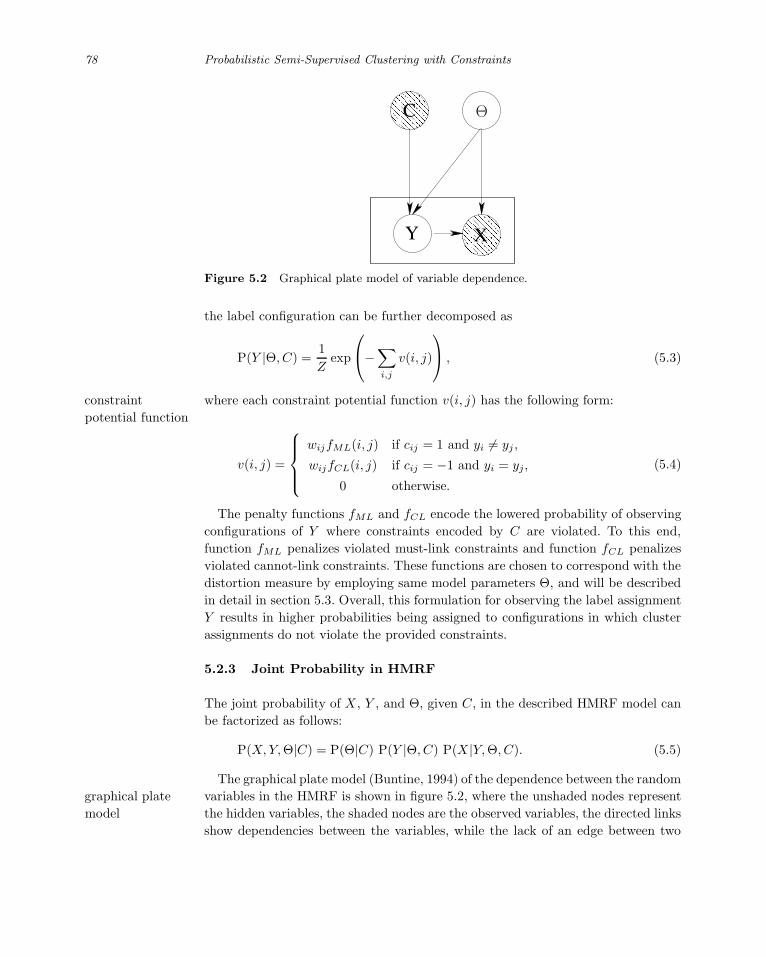
78 Probabilistic Semi-Supervised Clustering with Constraints
XY
C Θ
Figure 5.2 Graphical plate model of variable dependence.
the label configuration can be further decomposed as
P(Y |Θ, C) =1
Zexp
⎛
⎝−∑
i,j
v(i, j)
⎞
⎠ , (5.3)
where each constraint potential function v(i, j) has the following form:constraint
potential function
v(i, j) =
⎧⎪⎪⎨
⎪⎪⎩
wijfML(i, j) if cij = 1 and yi = yj ,
wijfCL(i, j) if cij = −1 and yi = yj,
0 otherwise.
(5.4)
The penalty functions fML and fCL encode the lowered probability of observing
configurations of Y where constraints encoded by C are violated. To this end,
function fML penalizes violated must-link constraints and function fCL penalizes
violated cannot-link constraints. These functions are chosen to correspond with the
distortion measure by employing same model parameters Θ, and will be described
in detail in section 5.3. Overall, this formulation for observing the label assignment
Y results in higher probabilities being assigned to configurations in which cluster
assignments do not violate the provided constraints.
5.2.3 Joint Probability in HMRF
The joint probability of X , Y , and Θ, given C, in the described HMRF model can
be factorized as follows:
P(X, Y, Θ|C) = P(Θ|C) P(Y |Θ, C) P(X |Y,Θ, C). (5.5)
The graphical plate model (Buntine, 1994) of the dependence between the random
variables in the HMRF is shown in figure 5.2, where the unshaded nodes representgraphical plate
model the hidden variables, the shaded nodes are the observed variables, the directed links
show dependencies between the variables, while the lack of an edge between two

5.2 HMRF Model for Semi-Supervised Clustering 79
variables implies conditional independence. The prior probability of Θ is assumed to
be independent of C. The probability of observing the label configuration Y depends
on the constraints C and current generative model parameters Θ. Observed data
points corresponding to variables X are generated using the model parameters
Θ based on cluster labels Y , independent of the constraints C. The variables X
are assumed to be mutually independent: each xi is generated individually from
a conditional probability distribution P(x|y, Θ). Then, the conditional probability
P(X |Y,Θ, C) can be written as
P(X |Y,Θ, C) = P(X |Y,Θ) =
n∏
i=1
p(xi|yi, Θ), (5.6)
where p(·|yi, Θ) is the parameterized probability density function for the yith
cluster, from which xi is generated. This probability density is related to the
clustering distortion measure dA, as described below in section 5.2.4.
From Eqs. 5.3, 5.5, and 5.6, it follows that maximizing the joint probability on
the HMRF is equivalent to maximizing
P(X, Y, Θ|C) = P(Θ)
(1
Zexp
⎛
⎝−∑
cij∈C
v(i, j)
⎞
⎠)( n∏
i=1
p(xi|yi, Θ)
). (5.7)
The joint probability in Eq. (5.7) has three factors. The first factor describes ajoint probability
factorization probability distribution over the model parameters preventing them from converg-
ing to degenerate values, thereby providing regularization. The second factor is the
conditional probability of observing a particular label configuration given the pro-
vided constraints, effectively assigning a higher probability to configurations where
the cluster assignments do not violate the constraints. Finally, the third factor is
the conditional probability of generating the observed data points given the labels
and the parameters: if maximum-likelihood (ML) estimation was performed on the
HMRF, the goal would have been to maximize this term in isolation.
Overall, maximizing the joint HMRF probability in (5.7) is equivalent to jointly
maximizing the likelihood of generating data points from the model and the
probability of label assignments that respect the constraints, while regularizing
the model parameters.
5.2.4 Semi-Supervised Clustering Objective Function on HMRF
Formulation 5.7 suggests a general framework for incorporating constraints into
clustering. The choice of the conditional probability p(x|y, Θ) in a particular
instantiation of the framework is directly connected to the choice of the distortion
measure appropriate for the clustering task.
When considering the conditional probability p(xi|yi, Θ)—the probability ofgenerative
probability for X generating a data point xi from the yith cluster—our attention is restricted to
probability densities from the exponential family, where the expectation parameter

80 Probabilistic Semi-Supervised Clustering with Constraints
corresponding to the yith cluster is μyi, the mean of the points of that cluster.
Using this assumption and the bijection between regular exponential distributions
and regular Bregman divergences (Banerjee et al., 2005b), the conditional density
for observed data can be represented as
p(xi|yi, Θ) =1
ZΘexp
(−dA(xi, μh)
), (5.8)
where dA(xi, μyi) is the Bregman divergence between xi and μyi
, corresponding to
the exponential density p, and ZΘ is the normalizer.2 Different clustering models
fall into this exponential form:
If xi and μyiare vectors in Euclidean space, and dA is the square of the L2
distance parameterized by a positive semidefinite weight matrix A (dA(xi, μyi) =
‖xi − μyi‖2
A), then the cluster conditional probability is a Gaussian with covariance
encoded by A−1 (Kearns et al., 1997);
If xi and μyiare probability distributions and dA is the KL divergence
(dA(xi, μyi) =
∑dm=1 xim log xim
μyim), then the cluster conditional probability is a
multinomial distribution (Dhillon and Guan, 2003).
The relation in Eq. 5.8 holds even if dA is not a Bregman divergence but
a directional distance measure like cosine distance. For example, if xi and μyi
are vectors of unit length and dA is one minus the dot-product of the vectors(dA(xi, μyi
) = 1 −Pd
m=1 ximμyim
‖xi‖‖μyi‖), then the cluster conditional probability is a
von Mises Fisher (vMF) distribution with unit concentration parameter (Banerjee
et al., 2005a), which is essentially the spherical analog of a Gaussian. The connection
between specific distortion measures studied in this chapter and their corresponding
cluster conditional probabilities is discussed in more detail in section 5.3.3.
Putting Eq. 5.8 into 5.7 and taking logarithms gives the following cluster objective
function, minimizing which is equivalent to maximizing the joint probability over
the HMRF in Eq. 5.7:
Jobj =∑
xi∈X
dA(xi, μyi) +
∑
cij∈C
v(i, j) − log P(Θ) + log Z + n log ZΘ. (5.9)
Thus, the task is to minimize Jobj over the hidden variables Y and Θ (note that
given Y , the means M = (μ1, . . . , μK) are uniquely determined).
2. When A = I (identity matrix), the bijection result (Banerjee et al., 2005b) ensures thatthe normalizer ZΘ is 1. In general, there are additional multiplicative terms that dependonly on x, and hence can be safely ignored for parameter estimation purposes.

5.3 HMRF-KMeans Algorithm 81
5.3 HMRF-KMeans Algorithm
Since the cluster assignments and the generative model parameters are unknown in
a clustering setting, minimizing Eq. 5.9 is an “incomplete-data problem”. A popular
solution technique for such problems is the expectation-maximization (EM) algo-
rithm (Dempster et al., 1977). The K-Means algorithm (MacQueen, 1967) is known
to be equivalent to the EM algorithm with hard clustering assignments, under cer-
tain assumptions (Kearns et al., 1997; Basu et al., 2002; Banerjee et al., 2005b). This
section describes a K-Means-type hard partitional clustering algorithm, HMRF-
KMeans, that finds a local minimum of the semi-supervised clustering objective
function Jobj in Eq. 5.9.
5.3.1 Normalizing Component Estimation
Before describing the details of the clustering algorithm, it is important to consider
the normalizing components: the MRF partition function logZ and the distortion
function normalizer logZΘ in Eq. 5.9. Estimation of the partition function cannot
be performed in closed form for most nontrivial dependency structures, and ap-
proximate inference methods must be employed for computing it (Wainwright and
Jordan, 2003).
Estimation of the distortion normalizer logZΘ depends on the distortion measurenormalizer
approximation dA used by the model. This chapter considers three parameterized distortion mea-
sures: parameterized squared Euclidean distance, parameterized cosine distance,
and parameterized Kullback-Leibler (KL) divergence. For Euclidean distance, ZΘ
can be estimated in closed form, and this estimation is performed while minimizing
the clustering objective function Jobj in Eq. 5.9. For the other distortion measures,
estimating the distortion normalizer ZΘ cannot be performed in closed form, and
approximate inference must be again used (Banerjee et al., 2005a).
Since approximate inference methods can be very expensive computationally,
two simplifying assumptions can be made: the MRF partition function may be
considered to be constant in the clustering process, and the distortion normalizer
may be assumed constant for all distortion measures that do not provide its closed-
form estimate. With these assumptions, the objective function Jobj in Eq. 5.9 no
longer exactly corresponds to a joint probability on an HMRF. However, minimizing
this simplified objective has been shown to work well empirically (Bilenko et al.,
2004; Basu et al., 2004b). However, if in some applications it is important to preserve
the semantics of the underlying joint probability model, then the normalizers Z and
ZΘ must be estimated by approximate inference methods.

82 Probabilistic Semi-Supervised Clustering with Constraints
5.3.2 Parameter Priors
Following the definition of Θ in section 5.2.1, the prior term log P(Θ) in (5.9) and
the subsequent equations can be factored as follows:
log P(Θ) = log(P(A)P(M)
)= log P(A) + PM ,
where the distortion parameters A are assumed to be independant of the cluster
centroids M = (μ1, . . . , μK), and uniform priors are considered over the cluster
centroids (leading to the constant term PM ). For different distortion measures,
parameter values may exist that lead to degenerate solutions of the optimization
problem. For example, for squared Euclidean distance, the zero matrix A = 0 is
one such solution. To prevent degenerate solutions, P(A) is used to regularize the
parameter values using a prior distribution.
If the standard Gaussian prior was used on the parameters of the distortion
function, it would allow the parameters to take negative values. Since it is desirableRayleigh prior
to constrain the parameter values to be non-negative, it is more appropriate to use
the Rayleigh distribution (Papoulis and Pillai, 2001). Assuming independence of
the parameters aij ∈ A, the prior term based on the Rayleigh distribution is the
following:
P(A) =∏
aij∈A
aij exp(−a2
ij
s2
)
s2, (5.10)
where s is the width parameter.
5.3.3 Adaptive Distortion Measures
Selecting an appropriate distortion measure dA for a clustering task typically
involves knowledge about properties of the particular domain and data set. For
example, squared Euclidean distance is most appropriate for low-dimensional data
with distribution close to Gaussian, while cosine distance best captures distance
between data described by vectors in high-dimensional space where differences in
angles are important but vector lengths are not.
Distortion measures from two families are considered in this chapter: Bregman
divergences (Banerjee et al., 2005b), which include parameterized squared Euclideandistortion
measure selection distance and KL divergence, and distortion measures based on directional similarity
functions, which include cosine similarity and Pearson’s correlation (Mardia and
Jupp, 2000). The distortion measure for directional functions is chosen to be the
directional similarity measure subtracted from a constant sufficiently large so that
the resulting value is non-negative. For both Bregman divergences and cosine
distance, there exist efficient K-Means-type iterative relocation algorithms that
minimize the corresponding clustering objective (Banerjee et al., 2005a,b), which
the HMRF-KMeans naturally extends to incorporate pairwise supervision.

5.3 HMRF-KMeans Algorithm 83
For many realistic data sets, off-the-shelf distortion measures may fail to capture
the correct notion of similarity in a clustering setting. While some unsupervised
measures like squared Euclidean distance and Pearson’s distance attempt to correct
distortion estimates using the global mean and variance of the data set, these mea-
sures may still fail to estimate distances accurately if the attributes’ true contribu-
tions to the distance are not correlated with their variance. Several semi-supervised
clustering approaches exist that incorporate adaptive distortion measures, including
parameterizations of Jensen-Shannon divergence (Cohn et al., 2003) and squared
Euclidean distance (Bar-Hillel et al., 2003; Xing et al., 2003). However, these tech-
niques use only constraints to learn the distortion measure parameters and exclude
unlabeled data from the parameter learning step, as well as separate the parameter
learning step from the clustering process.
Going a step further, the HMRF model provides an integrated framework
which incorporates both learning the distortion measure parameters and constraint-adaptive
distortion
measure
sensitive cluster assignments. In HMRF-KMeans, the parameters of the distortion
measure are learned iteratively as the clustering progresses, utilizing both unlabeled
data and pairwise constraints. The parameters are modified to decrease the param-
eterized distance between violated must-linked constraints and increase it between
violated cannot-link constraints, while allowing constraint violations if they accom-
pany a more cohesive clustering.
This section presents three examples of distortion functions and their parame-
terizations for use with HMRF-KMeans: squared Euclidean distance, cosine dis-
tance, and KL divergence. Through parameterization, each of these functions be-
comes adaptive in a semi-supervised clustering setting, permitting clusters of vary-
ing shapes.
Once a distortion measure is chosen for a given domain, the functions fML
and fCL, introduced in section 5.2.2 for penalizing must-link and cannot-linkconstraint
potential function constraint violations, respectively, must be defined. These functions typically follow
a functional form identical or similar to the corresponding distortion measure, and
are chosen as follows:
fML(i, j) = ϕ(i, j), (5.11)
fCL(i, j) = ϕmax − ϕ(i, j), (5.12)
where ϕ : X × X → R+ is a non-negative function that penalizes constraint
violation, and ϕmax is an upper bound on the maximum value of ϕ over any pair
of points in the data set; examples of such bounds for specific distortion functions
are shown below. The function ϕ is chosen to correlate with the distortion measure,
assigning higher penalties to violations of must-link constraints between points that
are distant with respect to the current parameter values of the distortion measure.
Conversely, penalties for violated cannot-link constraints are higher for points that
have low distance between them. With this formulation of the penalty functions,
constraint violations lead to changes in the distortion measure parameters that

84 Probabilistic Semi-Supervised Clustering with Constraints
attempt to mend the violations. The ϕ function for different clustering distortion
measures is discussed in the following sections.
Accordingly, the potential function v(i, j) in (5.4) becomes
v(i, j) =
⎧⎪⎪⎨
⎪⎪⎩
wijϕ(xi, xj) if cij = 1 and yi = yj
wij
(ϕmax − ϕ(xi, xj)
)if cij = −1 and yi = yj
0 otherwise
, (5.13)
and the objective function for semi-supervised clustering in (5.9) can be expressed
as
Jobj =∑
xi∈X
dA(xi, μ(i)) +∑
(xi,xj)∈CML
s.t. yi =yj
wijϕ(xi, xj)
+∑
(xi,xj)∈CCL
s.t. yi=yj
wij
(ϕmax − ϕ(xi, xj)
)− log P(A) + n log ZΘ. (5.14)
Note that as discussed in section 5.3.1, the MRF partition function term log Z has
been dropped from the objective function.
5.3.3.1 Parameterized Squared Euclidean Distance
Squared Euclidean distance is parameterized using a symmetric positive-definite
matrix A as follows:
deucA(xi, xj) = ‖xi − xj‖2
A = (xi − xj)T A(xi − xj). (5.15)
This form of the parameterized squared Euclidean distance is equivalent to Maha-
lanobis distance with an arbitrary positive semidefinite weight matrix A in place
of the inverse covariance matrix, and it was previously used for semi-supervised
clustering by (Xing et al., 2003) and (Bar-Hillel et al., 2003). Such formulation can
also be viewed as a projection of every instance x onto a space spanned by A1/2:
x→A1/2x.
To use parameterized squared Euclidean distance as the adaptive distortion mea-
sure for clustering, the ϕ function that penalizes constraint violations is defined
as ϕ(xi, xj) = deucA(xi, xj). One possible initialization of the upper bound for
cannot-link penalties is ϕmaxeucA
=∑
(xi,xj)∈CCLdeucA
(xi, xj), which guarantees that
the penalty is always positive. Using these definitions along with (5.14), the fol-
lowing objective function is obtained for semi-supervised clustering with adaptive
squared Euclidean distance:

5.3 HMRF-KMeans Algorithm 85
JeucA=
∑
xi∈X
deucA(xi, μ(i)) +
∑
(xi,xj)∈CML
s.t. yi =yj
wijdeucA(xi, xj)
+∑
(xi,xj)∈CCL
s.t. yi=yj
wij
(ϕmax
eucA− deucA
(xi, xj))− log P(A) − n log det(A).
(5.16)
Note that as discussed in section 5.3.1, the log ZΘ term is computable in closed-
form for a Gaussian distribution with covariance matrix A−1, which is the underly-
ing cluster conditional probability distribution for parameterized squared Euclidean
distance. The log det(A) term (5.16) corresponds to the log ZΘ term in this case.
5.3.3.2 Parameterized Cosine Distance
Cosine distance can be parameterized using a symmetric positive-definite matrix
A, which leads to the following distortion measure:
dcosA(xi, xj) = 1 − xT
i Axj
‖xi‖A‖xj‖A. (5.17)
Because for realistic high-dimensional domains computing the full matrix A would
be computationally expensive, a diagonal matrix is considered in this case, such
that a = diag(A) is a vector of positive weights.
To use parameterized squared Euclidean distance as the adaptive distortion
measure for clustering, the ϕ function is defined as ϕ(xi, xj) = dcosA(xi, xj). Using
this definition along with Eq. 5.14, and setting ϕmax = 1 as an upper bound on
ϕ(xi, xj), the following objective function is obtained for semi-supervised clustering
with adaptive cosine distance:
JcosA=
∑
xi∈X
dcosA(xi, μ(i)) +
∑
(xi,xj)∈CML
s.t. yi =yj
wijdcosA(xi, xj)
+∑
(xi,xj)∈CCL
s.t. yi=yj
wij
(1 − dcosA
(xi, xj))− log P(A). (5.18)
Note that as discussed in section 5.3.1, it is difficult to compute the log ZΘ term
in closed form for parameterized cosine distance. So, the simplifying assumption is
made that log ZΘ is constant during the clustering process and the normalizer term
is dropped from (5.18).

86 Probabilistic Semi-Supervised Clustering with Constraints
5.3.3.3 Parameterized KL Divergence
In certain domains, data are described by probability distributions, e.g., text
documents can be represented as probability distributions over words generated
by a multinomial model (Pereira et al., 1993). KL divergence is a widely used
distance measure for such data: dKL(xi, xj) =∑d
m=1 xim log xim
xjm, where xi and
xj are probability distributions over d events:∑d
m=1 xim =∑d
m=1 xjm = 1. In
previous work, Cohn et al. (2003) parameterized KL divergence by multiplying the
mth component by a weight γm: d′KL(xi, xj) =∑d
m=1 γmxim log xim
xjm.
In our framework, KL distance is parameterized using a diagonal matrix A, where
a = diag(A) is a vector of positive weights. This parameterization of KL by AI divergence
converts it to I divergence, a function that also belongs to the class of Bregman
divergences (Banerjee et al., 2005b). I divergence has the form: dI(xi, xj) =∑dm=1 xim log xim
xjm− ∑d
m=1(xim − xjm), where xi and xj no longer need to be
probability distributions but can be any non-negative vectors.3 The following
parameterization of KL is used:
dIA(xi, xj) =
d∑
m=1
amxim logxim
xjm−
d∑
m=1
am(xim − xjm), (5.19)
which can be interpreted as scaling every component of the original probability
distribution by a weight contained in the corresponding component of A, and then
taking I divergence between the transformed distributions.
For every distortion measure, the clustering framework described in section 5.2.4
requires defining an appropriate constraint potential function that is symmetric,
since the constraint pairs are unordered. To meet this requirement, a sum of
weighted I divergences from xi and xj to the mean vectorxi+xj
2 is used. This
parameterized I divergence to the mean, dIMA, is analogous to Jensen-Shannon
divergence (Cover and Thomas, 1991), the symmetric KL divergence to the mean,
and is defined as follows:
dIMA(xi, xj) =
d∑
m=1
am
(xim log
2xim
xim + xjm+ xjm log
2xjm
xim + xjm
). (5.20)
To use parameterized squared Euclidean distance as the adaptive distortion
measure for clustering, the ϕ function is defined as ϕ(xi, xj) = dIMA(xi, xj). Using
this definition along with Eq. 5.14, the following objective function is obtained for
semi-supervised clustering with adaptive KL distance:
3. For probability distributions, I divergence and KL divergence are equivalent.

5.3 HMRF-KMeans Algorithm 87
JIA=
∑
xi∈X
dIA(xi, μ(i)) +
∑
(xi,xj)∈CML
s.t. yi =yj
wijdIMA(xi, xj)
+∑
(xi,xj)∈CCL
s.t. yi=yj
wij
(dmax
IMA− dIMA
(xi, xj))− log P(A). (5.21)
The upper bound dmaxIMA
can be initialized as dmaxIMA
=∑d
m=1 am, which follows
from the fact that unweighted Jensen-Shannon divergence is bounded above by
1 (Lin, 1991).
Note that as discussed in section 5.3.1, it is difficult to compute the log ZΘ term in
closed form for parameterized KL distance. So, analogously to the parameterized
cosine distance case, the simplifying assumption is made that log ZΘ is constant
during the clustering process and that term is dropped from Eq. 5.21.
5.3.4 EM Framework
As discussed earlier in this section, Jobj can be minimized by a K-Means-type
iterative algorithm HMRF-KMeans. The outline of the algorithm is presented in
algorithm 5.1. The basic idea of HMRF-KMeans is as follows: the constraints
are used to get a good initialization of the clustering. Then in the E step, given
the current cluster representatives, every data point is reassigned to the cluster
which minimizes its contribution to Jobj. In the M step, the cluster representatives
M = (μ1, . . . , μK) are re-estimated from the cluster assignments to minimize Jobj
for the current assignment. The clustering distortion measure dA is subsequently
updated in the M step to reduce the objective function by modifying the parameters
A of the distortion measure.
Note that this corresponds to the generalized EM algorithm (Neal and Hinton,generalized EM
1998; Dempster et al., 1977), where the objective function is reduced but not
necessarily minimized in the M step. Effectively, the E step minimizes Jobj over
cluster assignments Y , the M step (A) minimizes Jobj over cluster representatives
M , and the M step (B) reduces Jobj over the parameters A of the distortion measure
dA. The E step and the M step are repeated till a specified convergence criterion is
reached. The specific details of the E step and M step are discussed in the following
sections.
5.3.5 Initialization
Good initial centroids are essential for the success of partitional clustering algo-
rithms such as K-Means. Good centroids are inferred from both the constraints
and unlabeled data during initialization. For this, a two-stage initialization process
is used.

88 Probabilistic Semi-Supervised Clustering with Constraints
Algorithm 5.1 HMRF-KMeans algorithm.
Neighborhood Inference At first, the transitive closure of the must-link con-
straints is taken to get connected components consisting of points connected by
must-links. Let there be λ connected components, which are used to create λ neigh-
borhoods. These correspond to the must-link neighborhoods in the MRF over the
hidden cluster variables.
Cluster Selection The λ neighborhood sets produced in the first stage are used
to initialize the HMRF-Means algorithm. If λ = K, λ cluster centers are initialized
with the centroids of all the λ neighborhood sets. If λ < K, λ clusters are initialized
from the neighborhoods, and the remaining K−λ clusters are initialized with points
obtained by random perturbations of the global centroid of X . If λ > K, a weighted
variant of farthest-first traversal (Hochbaum and Shmoys, 1985) is applied to the
centroids of the λ neighborhoods, where the weight of each centroid is proportional
to the size of the corresponding neighborhood. Weighted farthest-first traversal
selects neighborhoods that are relatively far apart as well as large in size, and
the chosen neighborhoods are set as the K initial cluster centroids for HMRF-
KMeans.
Overall, this two-stage initialization procedure is able to take into account both
unlabeled and labeled data to obtain cluster representatives that provide a good
initial partitioning of the data set.
5.3.6 E Step
In the E step, assignments of data points to clusters are updated using the current
estimates of the cluster representatives. In the general unsupervised K-Means
algorithm, there is no interaction between the cluster labels, and the E step is
a simple assignment of every point to the cluster representative that is nearest to

5.3 HMRF-KMeans Algorithm 89
it according to the clustering distortion measure. In contrast, the HMRF model
incorporates interaction between the cluster labels defined by the random field
over the hidden variables. As a result, computing the assignment of data points to
cluster representatives to find the global minimum of the objective function, given
the cluster centroids, is NP-hard in any nontrivial HMRF model, similar to other
graphical models such as MRFs and belief networks (Roth, 1996).
There exist several techniques for computing cluster assignments that approx-
imate the optimal solution in this framework, e.g., iterated conditional modesgreedy ICM
assignment (ICM) (Besag, 1986; Zhang et al., 2001), belief propagation (Pearl, 1988; Segal
et al., 2003b), and linear programming relaxation (Kleinberg and Tardos, 1999).
ICM is a greedy strategy that sequentially updates the cluster assignment of each
point, keeping the assignments for the other points fixed. In many settings it has
comparable performance to more expensive global approximation techniques, but is
computationally more efficient; it has been compared with several other approaches
by Bilenko and Basu (2004), while in more recent work Lange et al. (2005) have
described an alternative efficient method based on the mean-field approximation.
ICM performs sequential cluster assignment for all the points in random order. Each
point xi is assigned to the cluster representative μh that minimizes the point’s con-
tribution to the objective function Jobj(xi, μh):
Jobj(xi, μh) = dA(xi, μh) +∑
(xi,xj)∈CiML
s.t. yi =yj
wijϕ(xi, xj)
+∑
(xi,xj)∈CiCL
s.t. yi=yj
wij
(ϕmax − ϕ(xi, xj)
)− log P(A), (5.22)
where CiML and Ci
CL are the subsets of CML and CCL respectively in which xi
appears in the constraints. The optimal assignment for every point minimizes the
distortion between the point and its cluster representative (first term of Jobj) along
with incurring a minimal penalty for constraint violations caused by this assignment
(second and third terms of Jobj). After all points are assigned, they are randomly
reordered, and the assignment process is repeated. This process proceeds until no
point changes its cluster assignment between two successive iterations.
Overall, the assignment of points to clusters incorporates pairwise supervision by
discouraging constraint violations proportionally to their severity, which guides the
algorithm toward a desirable partitioning of the data.
5.3.7 M Step
The M step of the algorithm consists of two parts: centroid re-estimation and
distortion measure parameter update.

90 Probabilistic Semi-Supervised Clustering with Constraints
5.3.7.1 M Step (A): Centroid Re-estimation
In the first part of the M step, the cluster centroids M are re-estimated from points
currently assigned to them, to decrease the objective function Jobj in Eq. 5.9. For
Bregman divergences and cosine distance, the cluster representative calculated in
the M step of the EM algorithm is equivalent to the expectation value over the
points in that cluster, which is equal to their arithmetic mean (Banerjee et al.,
2005a,b). Additionally, it has been experimentally demonstrated that for clustering
with distribution-based measures, e.g., KL divergence, smoothing cluster represen-
tatives by a prior using a deterministic annealing schedule leads to considerable
improvements (Dhillon and Guan, 2003). With smoothing controlled by a positive
parameter α, each cluster representative μh is estimated as follows when dIAis the
distortion measure:
μ(IA)h =
1
1 + α
(∑xi∈Xh
xi
|Xh|+
α
n1
). (5.23)
For directional measures, each cluster representative is the arithmetic mean
projected onto unit sphere (Banerjee et al., 2005a). Taking the distortion parameters
into account, centroids are estimated as follows when dcosAis the distortion measure:
μ(cosA)h
‖μ(cosA)h ‖A
=
∑xi∈Xh
xi
‖∑xi∈Xhxi‖A
. (5.24)
5.3.7.2 M Step (B): Update of Distortion Parameters
In the second part of the M step, the parameters of the parameterized distortion
measure are updated to decrease the objective function. In general, for parameter-
ized Bregman divergences or directional distances with general parameter priors,
it is difficult to attain a closed-form update for the parameters of the distortion
measure that can minimize the objective function.4 Gradient descent provides an
alternative avenue for learning the distortion measure parameters.
For squared Euclidean distance, a full parameter matrix A is updated during
gradient descent using the rule: A = A + η∂JeucA
∂A (where η is the learning rate).gradient update
for full A Using (5.16),∂JeucA
∂A can be expressed as
4. For the specific case of parameterized squared Euclidean distance, a closed-form updateof the parameters can be obtained (Bilenko et al., 2004).

5.3 HMRF-KMeans Algorithm 91
∂JeucA
∂A=
∑
xi∈X
∂deucA(xi, μ(i))
∂A+
∑
(xi,xj)∈CML
s.t. yi =yj
wij∂deucA
(xi, xj)
∂A
+∑
(xi,xj)∈CCL
s.t. yi=yj
wij
[∂ϕmax
eucA
∂A− ∂deucA
(xi, xj)
∂A
]− ∂ log P(A)
∂A− n
∂ log det(A)
∂A.
(5.25)
The gradient of the parameterized squared Euclidean distance is given by
∂deucA(xi, xj)
∂A= (xi − xj)(xi − xj)
T .
The derivative of the upper bound ϕmaxeucA
is∂ϕmax
eucA
∂A =∑
(xi,xj)∈CCL(xi −xj)(xi −
xj)T if ϕmax
eucAis computed as described in section 5.3.3.1.5
When Rayleigh priors are used on the set of parameters A, the partial derivative
of the log-prior with respect to every individual parameter am ∈ A, ∂ log P(A)∂am
, is
given by
∂ log P(A)
∂am=
1
am− am
s2. (5.26)
The gradient of the distortion normalizer log det(A) term is as follows:
∂ log det(A)
∂A= 2A−1 − diag(A−1). (5.27)
For parameterized cosine distance and KL divergence, a diagonal parameter
matrix A is considered, where a = diag(A) is a vector of positive weights. Duringgradient update
for diagonal A gradient descent, each weight am is individually updated as am = am + η∂Jobj
∂am(η
is the learning rate). Using (5.14),∂Jobj
∂amcan be expressed as
∂Jobj
∂am=
∑
xi∈X
∂dA(xi, μ(i))
∂am+
∑
(xi,xj)∈CML
s.t. yi =yj
wij∂ϕ(xi, xj)
∂am
+∑
(xi,xj)∈CCL
s.t. yi=yj
wij
[∂ϕmax
∂am− ∂ϕ(xi, xj)
∂am
]− ∂ log P(A)
∂am. (5.28)
5. In practice, one can initialize ϕmaxeucA
with a sufficiently large constant, which wouldmake its derivative zero. Accordingly, an extra condition must be then inserted intothe algorithm to guarantee that penalties for violated cannot-link constraints are nevernegative, in which case the constant must be increased.

92 Probabilistic Semi-Supervised Clustering with Constraints
Calculation of the gradient∂Jobj
∂amfor cosine distance and KL divergence, which
are parameterized by a diagonal matrix A, needs the gradients of the corresponding
distortion measures and constraint potential functions, which are
∂dcosA(xi, xj)
∂am=
ximxjm‖xi‖A‖xj‖A − xTi Axj
x2im‖xj‖2
A+x2jm‖xi‖2
A
2‖xi‖A‖xj‖A
‖xi‖2A‖xj‖2
A
,
∂dIA(xi, xj)
∂am= xim log
xim
xjm− (xim − xjm),
∂dIMA(xi, xj)
∂am= xim log
2xim
xim + xjm+ xjm log
2xjm
xim + xjm, (5.29)
while the gradient of the upper bound ∂ϕmax
∂amis 0 for parameterized cosine and 1 for
parameterized KL divergence, as follows from the expressions for these constants
in sections 5.3.3.2 and 5.3.3.3.
Overall, the distance learning step results in modifying the distortion measure
so that data points in violated must-link constraints are brought closer together,
while points in violated cannot-link constraints are pulled apart. This process leads
to a transformed data space that facilitates partitioning of the unlabeled data,
by attempting to mend the constraint violations as well as reflecting the natural
variance in the data. See part IV (chapters 15–17) for several alternative techniques
that change the data representation leading to better estimates of similarity between
data points.
5.3.8 Convergence of HMRF-KMeans
The HMRF-KMeans algorithm alternates between updating the assignment of
points to clusters, and updating the parameters. Since all updates ensure a de-
crease in the objective function, each iteration of HRMF-KMeans monotonically
decreases the objective function. Let us inspect each step in the update to ensure
that this is indeed the case.
For analyzing the cluster assignment step, let us consider Eq. 5.14. Each point xi
moves to a new cluster h only if the following component, contributed by the point
xi, is decreased with the move:
dA(xi, μ(i))+∑
(xi,xj)∈CiML
s.t. yi =yj
wijϕ(xi, xj)+∑
(xi,xj)∈CiCL
s.t. yi=yj
wij
(ϕmax−ϕ(xi, xj)
)−log P(A).
Given a set of centroids and distortion parameters, the new cluster assignment of
points will decrease Jobj or keep it unchanged.
For analyzing the centroid re-estimation step, let us consider an equivalent form
of Eq. 5.14:

5.4 Active Learning for Constraint Acquisition 93
Jobj =
K∑
h=1
∑
xi∈Xh
dA(xi, μh) +∑
(xi,xj)∈CiML
s.t. yi =yj
wijϕ(xi, xj)
+∑
(xi,xj)∈CiCL
s.t. yi=yj
wij
(ϕmax − ϕ(xi, xj)
)− log P(A). (5.30)
Each cluster centroid μh is re-estimated by taking the mean of the points in the
partition Xh, which minimizes the component∑
xi∈XhdA(xi, μh) of Jobj in Eq. 5.30
contributed by the partition Xh. The constraint potential and the prior term in the
objective function do not take a part in centroid re-estimation, because they are
not explicit functions of the centroid. So, given the cluster assignments and the
distortion parameters, Jobj will decrease or remain the same in this step.
For the parameter estimation step, the gradient-descent update of the parameters
in M step (B) decreases Jobj or keeps it unchanged. Hence the objective function
decreases after every cluster assignment, centroid re-estimation, and parameter
re-estimation step. Now, note that the objective function is bounded below by
a constant: being the negative log likelihood of a probabilistic model with the
normalizer terms, Jobj is bounded below by zero. Even without the normalizers,
the objective function is bounded below by zero, since the distortion and potential
terms are non-negative due to the fact that A is positive definite. Since Jobj is
bounded below, and HMRF-KMeans results in a decreasing sequence of objective
function values, the value sequence must have a limit. The limit in this case will
be a fixed point of Jobj since neither updating the assignments nor the parameters
can further decrease the value of the objective function. As a result, the HMRF-
KMeans algorithm will converge to a fixed point of the objective. In practice,
convergence can be determined if subsequent iterations of HMRF-KMeans result
in insignificant changes in Jobj.
5.4 Active Learning for Constraint Acquisition
In the semi-supervised setting where training data are not already available, getting
constraints on pairs of data points may be expensive. In this section an active
learning scheme for the HMRF model is presented, which can improve clustering
performance with as few queries as possible. Formally, the scheme has access to a
(noiseless) oracle that can assign a must-link or cannot-link label to a given pair
(xi, xj), and it can pose a constant number of queries to the oracle.6
In order to get pairwise constraints that are more informative than random in
6. The oracle can also give a don’t-know response to a query, in which case that responseis ignored (pair not considered as a constraint) and that query is not posed again later.

94 Probabilistic Semi-Supervised Clustering with Constraints
the HMRF model, an active learning scheme for selecting pairwise constraints using
the farthest-first traversal scheme is developed. In farthest-first traversal, a startingfarthest-first
traversal point is first selected at random. Then, the next point farthest from it is chosen and
added to the traversed set. After that, the next point farthest from the traversed
set (using the standard notion of distance from a set: d(x, S) = minx′∈S d(x, x′))is selected, and so on. Farthest-first traversal gives an efficient approximation of
the K-center problem (Hochbaum and Shmoys, 1985), and has also been used to
construct hierarchical clusterings with performance guarantees at each level of the
hierarchy (Dasgupta, 2002).
Basu et al. (2002) observed that initializing K-Means with centroids esti-
mated from a set of labeled examples for each cluster gives significant perfor-
mance improvements. Under certain generative model-based assumptions, one cangood
initialization for
K-Means
connect the mixture of Gaussians model to K-Means with squared Euclidean dis-
tance (Kearns et al., 1997). A direct calculation using Chernoff bounds shows that
if a particular cluster with an underlying Gaussian model is seeded with points
drawn independently at random from the corresponding Gaussian distribution, the
deviation of the centroid estimates falls exponentially with the number of seeds;
hence seeding results in good initial centroids. Since good initial centroids are very
critical for the success of greedy algorithms such as K-Means, the same principle
is followed for the pairwise case: the goal is to get as many points as possible per
cluster (proportional to the actual cluster size) by asking pairwise queries, so that
HMRF-KMeans is initialized from a very good set of centroids. The proposed
active learning scheme has two phases, Explore and Consolidate, which are
discussed next.
5.4.1 Exploration
The Explore phase explores the given data using farthest-first traversal to get K
pairwise disjoint non-null neighborhoods as fast as possible, with each neighborhood
belonging to a different cluster in the underlying clustering of the data. Note that
even if there is only one point per neighborhood, this neighborhood structure
defines a correct skeleton of the underlying clustering. Our algorithm Exploreform skeleton of
neighborhoods (algorithm 5.2) uses farthest-first traversal for getting a skeleton structure of the
neighborhoods, and terminates when it has run out of queries, or when at least
one point from all the clusters has been labeled. In the latter case, active learning
enters the consolidation phase.
5.4.2 Consolidation
The basic idea in Consolidate (algorithm 5.3) is as follows: since there is at least
one labeled point from all the clusters, the proper neighborhood of any unlabeled
point x can be determined within a maximum of (K − 1) queries. The queries willconsolidate
neighborhoods be formed by taking a point y from each of the neighborhoods in turn and asking
for the label on the pair (x, y) until a must-link is obtained. Either a must-link reply

5.4 Active Learning for Constraint Acquisition 95
Algorithm 5.2 Explore
is obtained in (K − 1) queries, or it can be inferred that the point is must-linked
to the remaining neighborhood. Note that it is practical to sort the neighborhoods
in increasing order of the distance of their centroids from x so that the correct
must-link neighborhood for x is encountered sooner in the querying process.
Algorithm 5.3 Consolidate
Input: Set of data points X = (x1, . . . , xn), access to an oracle thatanswers pairwise queries, number of clusters K, total numberof queries Q, K disjoint neighborhoods corresponding to trueclustering of X with at least one point per neighborhood.
Output: K disjoint neighborhoods corresponding to the trueclustering of X with higher number of points per neighborhood.
Method:
1. Estimate centroids (µ1, . . . , µK) of each of the neighborhoods2. While queries are allowed2a. randomly pick a point x not in the existing neighborhoods2b. sort the indices h with increasing distances ‖x − µh‖
2
2c. for h = 1 to K
query x with each of the neighborhoods in sorted ordertill a must-link is obtained, add x to that neighborhood
When the right number of clusters K is not known to the clustering algorithm,
K is also unknown to the active learning scheme. In this case, only Explore is
used while queries are allowed. Explore will keep discovering new clusters as fast
as it can. When it has obtained all the clusters, it will not have any way of knowing
this. However, from this point onward, for every farthest-first x it draws from the
data set, it will always find a neighborhood that is must-linked to it. Hence, after

96 Probabilistic Semi-Supervised Clustering with Constraints
0
0.1
0.2
0.3
0.4
0.5
0.6
0.7
0.8
0 100 200 300 400 500
NM
I
Number of Constraints
KMeans-C-D-RKMeans-C-D
KMeans-CKMeans
Figure 5.3 Clustering results for Dcosa
on News-Different-3 data set.
0
0.1
0.2
0.3
0.4
0.5
0.6
0.7
0.8
0 100 200 300 400 500
NM
I
Number of Constraints
KMeans-C-D-RKMeans-C-D
KMeans-CKMeans
Figure 5.4 Clustering results for DIa onNews-Different-3 data set.
discovering all of the clusters, Explore will essentially consolidate the clusters too.
However, when K is known, it makes sense to invoke Consolidate since (1) it adds
points to clusters at a faster rate than Explore, and (2) it picks random samples
following the underlying data distribution, which is advantageous for estimating
good centroids (e.g., Chernoff bounds on the centroid estimates exist), while samples
obtained using farthest-first traversal may not have such properties.
5.5 Experimental Results
5.5.1 Data Sets
To demonstrate the effectiveness of our semi-supervised clustering framework,
we consider three data sets that have the characteristics of being sparse, high-
dimensional, and having a small number of points compared to the dimensionality
of the space. This is done for two reasons:
When clustering sparse high-dimensional data, e.g., text documents represented
using the vector space model, it is particularly difficult to cluster small data sets,
as observed by clustering researchers (Dhillon and Guan, 2003). The purpose of
performing experiments on these subsets is to scale down the sizes of the data sets
for computational reasons but at the same time not scale down the difficulty of the
tasks.
Clustering small number of sparse high-dimensional data points is a likely scenario
in realistic applications. For example, when clustering the search results in a
websearch engine like Vivısimo,7 typically the number of webpages that are being
clustered is on the order of hundreds. However the dimensionality of the feature
space, corresponding to the number of unique words in all the webpages, is on
the order of thousands. Moreover, each webpage is sparse, since it contains only a
7. http://www.vivisimo.com

5.5 Experimental Results 97
0
0.05
0.1
0.15
0.2
0.25
0.3
0.35
0 100 200 300 400 500
NM
I
Number of Constraints
KMeans-C-D-RKMeans-C-D
KMeans-CKMeans
Figure 5.5 Clustering results for Dcosa
on News-Related-3 data set.
0.05
0.1
0.15
0.2
0.25
0.3
0.35
0 100 200 300 400 500
NM
I
Number of Constraints
KMeans-C-D-RKMeans-C-D
KMeans-CKMeans
Figure 5.6 Clustering results for DIa onNews-Related-3 data set.
0
0.05
0.1
0.15
0.2
0.25
0.3
0.35
0 100 200 300 400 500
NM
I
Number of Constraints
KMeans-C-D-RKMeans-C-D
KMeans-CKMeans
Figure 5.7 Clustering results for Dcosa
on News-Similar-3 data set.
0
0.05
0.1
0.15
0.2
0.25
0.3
0.35
0 100 200 300 400 500
NM
I
Number of Constraints
KMeans-C-D-RKMeans-C-D
KMeans-CKMeans
Figure 5.8 Clustering results for DIa onNews-Similar-3 data set.
small number of all the possible words. On such data sets, clustering algorithms
can easily get stuck in local optima: in such cases it has been observed that there is
little relocation of documents between clusters for most initializations, which leads
to poor clustering quality after convergence of the algorithm (Dhillon and Guan,
2003). Supervision in the form of pairwise constraints is most beneficial in such
cases and may significantly improve clustering quality.
We derived three data sets from the 20-Newsgroups collection.8 This collection
has messages harvested from 20 different Usenet newsgroups, 1000 messages from
each newsgroup. From the original data set, a reduced data set was created by tak-
ing a random subsample of 100 documents from each of the 20 newsgroups. Three
data sets were created by selecting three categories from the reduced collection.
News-Similar-3 consists of three newsgroups on similar topics (comp.graphics,
comp.os.ms-windows, comp.windows.x) with significant overlap between clusters
due to cross-posting. News-Related-3 consists of three newsgroups on related top-
ics (talk.politics.misc, talk.politics.guns, and talk.politics.mideast).
News-Different-3 consists of articles posted in three newsgroups that cover differ-
ent topics (alt.atheism, rec.sport.baseball, sci.space) with well-separated
8. http://www.ai.mit.edu/people/jrennie/20Newsgroups

98 Probabilistic Semi-Supervised Clustering with Constraints
clusters. The vector-space model of News-Similar-3 has 300 points in 1864 dimen-
sions, News-Related-3 has 300 points in 3225 dimensions, and News-Different-3 had
300 points in 3251 dimensions. Since the overlap between topics in News-Similar-3
and News-Related-3 is significant, they are more challenging data sets than News-
Different-3.
All the data sets were preprocessed by stopword removal, TF-IDF weighting, re-
moval of very high-frequency and low-frequency words, etc., following the method-
ology of Dhillon et al. (Dhillon and Modha, 2001).
5.5.2 Clustering Evaluation
We used normalized mutual information (NMI) as our clustering evaluation mea-
sure. NMI is an external clustering validation metric that estimates the quality of
the clustering with respect to a given underlying class labeling of the data: it mea-
sures how closely the clustering algorithm could reconstruct the underlying label
distribution in the data (Strehl et al., 2000; Dom, 2001). If C is the random vari-
able denoting the cluster assignments of the points and K is the random variable
denoting the underlying class labels on the points (Banerjee et al., 2005a), then the
NMI measure is defined as
NMI =I(C; K)
(H(C) + H(K))/2, (5.31)
where I(X ; Y ) = H(X) − H(X |Y ) is the mutual information between the random
variables X and Y , H(X) is the Shannon entropy of X , and H(X |Y ) is the
conditional entropy of X given Y (Cover and Thomas, 1991). NMI effectively
measures the amount of statistical information shared by the random variables
representing the cluster assignments and the user-labeled class assignments of the
data points.
5.5.3 Methodology
We generated learning curves using 20 runs of twofold cross-validation for each
data set. For studying the effect of constraints in clustering, 50% of the data
set is set aside as the test set at any particular fold. The different points along
the learning curve correspond to constraints that are given as input to the semi-
supervised clustering algorithm. These constraints are obtained from the training
set corresponding to the remaining 50% of the data by randomly selecting pairs
of points from the training set, and creating must-link or cannot-link constraints
depending on whether the underlying classes of the two points are same or different.
Unit constraint costs W and W were used for all constraints, original and inferred,
since the data sets did not provide individual weights for the constraints. Based
on a few pilot studies, gradient step size η was chosen to have values η = 1.75 for
clustering with Dcosaand η = 1.0−8 for clustering with DIa
; weights were restricted
to be non-negative. In a realistic setting, these parameters could be tuned using

5.5 Experimental Results 99
cross-validation with a holdout set. The clustering algorithm was run on the whole
data set, but NMI was calculated only on the test set. The learning curve results
were averaged over the 20 runs.
5.5.4 Results and Discussion
We compared the proposed HMRF-KMeans algorithm with two ablations as well
as unsupervised K-Means clustering. The following variants were compared for
distortion measures Dcosaand DIa
as representatives for Bregman divergences and
directional measures respectively:
KMeans-I-C-D is the complete HMRF-KMeans algorithm that includes use
of supervised data in initialization (I) as described in section 5.3.5, incorporates
constraints in cluster assignments (C) as described in section 5.3.6, and performs
distance learning (D) as described in section 5.3.7;
KMeans-I-C is an ablation of HMRF-KMeans that uses pairwise supervision
for initialization and cluster assignments, but does not perform distance learning;
KMeans-I is a further ablation that only uses the constraints to initialize cluster
representatives;
KMeans is the unsupervised K-Means algorithm.
Figures 5.3, 5.5, and 5.7 demonstrate the results for experiments where weighted
cosine similarity Dcosawas used as the distortion measure, while figures 5.4, 5.6,
and 5.8 summarize experiments where weighted I divergence DIawas used.
As the results demonstrate, the full HMRF-KMeans algorithm outperforms the
unsupervised K-Means baseline as well as the ablated versions of HMRF-KMeans
for both Dcosaand DIa
. Relative performance of KMeans-I-C and KMeans-
I indicates that using supervision for initializing cluster representatives is highly
beneficial, while the constraint-sensitive cluster assignment step does not lead to
significant additional improvements for Dcosa. For DIa
, KMeans-I-C outperforms
KMeans-I on News-Different-3 (figure 5.4) and News-Similar-3 (figure 5.8) which
indicates that incorporating constraints in the cluster assignment process is useful
for these data sets. This result is reversed for News-Related-3 (figure 5.6), implying
that in some cases using constraints in the E step may be unnecessary, which agrees
with previous results on other domains (Basu et al., 2002). However, incorporating
supervised data in all the three stages of the algorithm in KMeans-I-C-D, namely
initialization, cluster assignment, and distance update, always leads to substantial
performance improvement.
As can be seen from results for 0 pairwise constraints in figures 5.3 through
5.8, distance learning is beneficial even in the absence of any pairwise constraints,
since it is able to capture the relative importance of the different attributes in the
unsupervised data. In the absence of supervised data or when no constraints are
violated, distance learning attempts to minimize the objective function by adjusting
the weights given the distortion between the unsupervised data points and their

100 Probabilistic Semi-Supervised Clustering with Constraints
corresponding cluster representatives.
In realistic application domains, supervision in the form of constraints would be in
most cases provided by human experts, in which case it is important that any semi-
supervised clustering algorithm performs well with a small number of constraints.
KMeans-I-C-D starts outperforming its variants and the unsupervised clustering
baseline early on in the learning curve, and is therefore a very appropriate algorithm
to use in actual semi-supervised data clustering systems.
Overall, our results show that the HMRF-KMeans algorithm effectively incor-
porates labeled and unlabeled data in three stages, each of which improves the
clustering quality.
5.6 Related Work
The problem of integrating limited supervision in clustering algorithms has been
studied by a number of authors in recent work. Early approaches to semi-supervised
clustering relied on incorporating penalties for violating constraints into the objec-
tive function, leading to algorithms that avoid clusterings in which constraints are
not satisfied. COP-KMeans is one such method where constraint violations are ex-
plicitly avoided in the assignment step of the K-Means algorithm (Wagstaff et al.,
2001; Wagstaff, 2002). Another method, proposed by Demiriz et al. (1999), uti-
lizes genetic algorithms to optimize an objective function that combines cluster
compactness and cluster purity and that decreases with constraint violations.
In subsequent work, several approaches have been proposed that consider semi-
supervised clustering within a probabilistic framework. Segal et al. (2003b) describe
a model for semi-supervised clustering with constraints that combines a binary
Markov network derived from pairwise protein interaction data and a naive Bayes
Markov network modeling gene expression data. Another probabilistic approach
described by Shental et al. (2004) incorporates must-link constraints via modeling
them as chunklets, sets of points known to belong to the same class, while cannot-
link constraints are utilized via potentials in a binary Markov network. HMRFs have
previously been used for image segmentation by Zhang et al. (2001), who have also
described an EM-based clustering algorithm. More recently, Lange et al. (2005)
proposed an approach that incorporates labeled and unlabeled data within an
HMRF-like model, while a mean field approximation method for posterior inference
is used in the E step of the algorithm. The HMRF framework described in this
chapter differs from these approaches in that it explicitly incorporates learning of
the distortion measure parameters within the clustering algorithm and facilitates
the use of diverse distance measures; however, a number of the proposed methods
could be integrated within the HMRF framework.
Spectral clustering methods—algorithms that perform clustering by decompos-
ing the pairwise affinity matrix derived from data—have been increasingly popular
recently (Weiss, 1999; Ng et al., 2002), and several semi-supervised approaches have
been developed within the spectral clustering framework. Kamvar et al. (2003) have

5.7 Conclusions 101
proposed directly injecting the constraints into the affinity matrix before subse-
quent clustering, while De Bie et al. (2004) reformulated the optimization problem
corresponding to spectral clustering by incorporating a separate label constraint
matrix. Additionally, spectral clustering methods can be viewed as variants of the
graph-cut approaches to clustering (Shi and Malik, 2000), a connection that mo-
tivated the correlation clustering method proposed by (Bansal et al., 2002), where
the constraints correspond to edge labels between vertices representing data points.
Another family of semi-supervised clustering methods has focused on modifying
the distance function employed by the clustering algorithm. In early work, Cohn
et al. (2003) proposed using a weighted variant of Jensen-Shannon divergence within
the EM clustering algorithm, with the weights learned using gradient descent based
on constraint violations. Within the family of hierarchical agglomerative clustering
algorithms, Klein et al. (2002) proposed modifying the squared Euclidean distance
using the shortest-path algorithm. Several researchers have proposed methods for
learning the parameters of the weighted Mahalanobis distance, a generalization of
Euclidean distance, within the context of semi-supervised clustering. Xing et al.
(2003) utilized convex optimization and iterative projections to learn the weight
matrix of Mahalanobis distance within K-Means clustering. Another approach
focused on parameterized Mahalanobis distance is the relevant component analysis
(RCA) algorithm proposed by Bar-Hillel et al. (2003), where convex optimization
is also used to learn the weight matrix.
Learning distance metrics within semi-supervised clustering relates to a large set
of approaches for transforming the data representation to make it more suitable
to a particular learning task. Within this book, part IV (chapters 15–17) describes
several advanced techniques for changing the geometry of the data space to obtain
better estimates of similarity between data points; integrating these methods with
clustering algorithms provides a number of promising avenues for future work.
5.7 Conclusions
In this chapter, a generative probabilistic framework for semi-supervised clustering
has been introduced. It relies on hidden random Markov fields (HMRFs) to utilize
both unlabeled data and supervision in the form of pairwise constraints during
the clustering process. The framework can be used with a number of distortion
(distance) measures, including Bregman divergences and directional measures, and
it facilitates training the distance parameters to adapt to specific data sets.
An algorithm HMRF-KMeans for performing clustering in this framework
has been presented that incorporates pairwise supervision in different stages of
the clustering: initialization, cluster assignment, and parameter estimation. Three
particular instantiations of the algorithm, based on different distortion measures,
have been discussed: squared Euclidean distance, which is common for clustering
low-dimensional data, and KL divergence and cosine distance, which are popular
for clustering high-dimensional directional data. Finally, a new method has been

102 Probabilistic Semi-Supervised Clustering with Constraints
presented for acquiring supervision from a user in the form of effective pairwise
constraints for semi-supervised clustering – such an active learning algorithm would
be useful in an interactive query-driven clustering framework.
The HMRF model can be viewed as a unification of constraint-based and
distance-based semi-supervised clustering approaches. It can be expanded to a
more general setting where every cluster has a corresponding distinct distortion
measure (Bilenko et al., 2004), leading to a clustering algorithm that can identify
clusters of different shapes. Empirical evaluation of the framework described in
this chapter can be found in several previous publications: active learning experi-
ments are discussed in (Basu et al., 2004a), while (Bilenko et al., 2004) and (Basu
et al., 2004b) contain results for low-dimensional and high-dimensional data sets
respectively, and (Bilenko and Basu, 2004) compares several approximate inference
methods for E Step discussed in section 5.3.6.
An important practical issue in using generative models for semi-supervised
learning is model selection. For semi-supervised clustering with constraints, the
key model selection issue is one of choosing the right number of clusters. One can
consider using a traditional model selection criterion suitable for the supervised
setting, or perform model selection by cross-validation. An alternative is to perform
model-selection using bounds on the test-set error rate such that valuable supervised
data are saved for learning. The PAC-MDL bounds (Blum and Langford, 2003)
provide such a tool that has been successfully applied to model selection for
clustering (Banerjee et al., 2005a), and can be readily extended to the semi-
supervised clustering setting. In fact, the semi-supervised clustering setting is
more natural since PAC-MDL bounds are applicable for transductive learning.
Alternative methods of model selection are a good topic for future research.

II Low-Density Separation


6 Transductive Support Vector Machines
Thorsten Joachims [email protected]
In contrast to learning a general prediction rule, V. Vapnik proposed the transduc-
tive learning setting where predictions are made only at a fixed number of known
test points. This allows the learning algorithm to exploit the location of the test
points, making it a particular type of semi-supervised learning problem. Transduc-
tive support vector machines (TSVMs) implement the idea of transductive learning
by including test points in the computation of the margin. This chapter will pro-
vide some examples for why the margin on the test examples can provide useful
prior information for learning, in particular for the problem of text classification.
The resulting optimization problems, however, are difficult to solve. The chapter re-
views exact and approximate optimization methods and discusses their properties.
Finally, the chapter discusses connections to other related semi-supervised learning
approaches like co-training and methods based on graph cuts, which can be seen
as solving variants of the TSVM optimization problem.
6.1 Introduction
The setting of transductive inference was introduced by Vapnik (e.g. (Vapnik,
1998)). As an example of a transductive learning task, consider the problem of
learning from relevance feedback in information retrieval (see (Baeza-Yates and
Ribeiro-Neto, 1999)). The user marks some documents returned by a search engine
in response to an initial query as relevant or irrelevant. These documents then serve
as a training set for a binary text classification problem. The goal is to learn a rule
that accurately classifies all remaining documents in the database according to their
relevance. Clearly, this problem can be thought of as a supervised learning problem.
But it is different from many other (inductive) learning problems in at least two
respects.
First, the learning algorithm does not necessarily have to learn a general rule,
but it only needs to predict accurately for a finite number of test examples (i.e.,
106 Transductive Support Vector Machines
the documents in the database). Second, the test examples are known a priori and
can be observed by the learning algorithm during training. This allows the learning
algorithm to exploit any information that might be contained in the location of
the test examples. Transductive learning is therefore a particular case of semi-
supervised learning, since it allows the learning algorithm to exploit the unlabeled
examples in the test set. The following focuses on this second point, while chapter 24
elaborates on the first point.
More formally, the transductive learning setting can be formalized as follows.1transductive
learning setting Given is a set
S = 1, 2, ..., n (6.1)
that enumerates all n possible examples. In our relevance feedback example from
above, there would be one index i for each document in the collection. We assume
that each example i is represented by a feature vector xi ∈ Rd. For text documents,
this could be a TFIDF vector representation (see e.g. (Joachims, 2002)), where
each document is represented by a scaled and normalized histogram of the words
it contains. The collection of feature vectors for all examples in S is denoted as
X = (x1,x2, ...,xn). (6.2)
For the examples in S, labels
Y = (y1,y2, ...,yn) (6.3)
are generated independently according to a distribution P (y1, ...,yn) =∏n
i=1 P (yi).
For simplicity, we assume binary labels yi ∈ −1, +1.As the training set, the learning algorithm can observe the labels of l randomly
selected examples Strain ⊂ S. The remaining u = n − l examples form the test set
Stest = S \ Strain.
Strain = l1, ..., ll Stest = u1, ..., uu (6.4)
When training a transductive learning algorithm L, it not only has access to the
training vectors Xtrain and the training labels Ytrain,
Xtrain = (xl1 ,xl2 , ...,xll) Ytrain = (yl1 ,yl2 , ...,yll), (6.5)
but also to the unlabeled test vectors
Xtest = (xu1 ,xu2 , ...,xul). (6.6)
The transductive learner uses Xtrain, Ytrain, and Xtest (but not the labels Ytest of
1. While several other, more general, definitions of transductive learning exist (Vapnik,1998; Joachims, 2002; Derbeko et al., 2003), this one was chosen for the sake of simplicity.

6.1 Introduction 107
the test examples) to produce predictions,
Y ∗test = (y∗
u1,y∗
u2, ...,y∗
uu), (6.7)
for the labels of the test examples. The learner’s goal is to minimize the fraction of
erroneous predictions,
Errtest(Y∗test) =
1
u
∑
i∈Stest
δ0/1(y∗i ,yi), (6.8)
on the test set. δ0/1(a, b) is zero if a = b, otherwise it is one.
At first glance, the problem of transductive learning may not seem profoundly
different from the usual inductive setting. One could learn a classification rule based
on the training data and then apply it to the test data afterward. However, a crucial
difference is that the inductive strategy would ignore any information potentially
conveyed in Xtest.
What information do we get from studying the test sample Xtest and how could
we use it? The fact that we deal with only a finite set of points means that the
hypothesis space H of a transductive learner is necessarily finite — namely, all
vectors −1, +1n. Following the principle of structural risk minimization (Vapnik,structural risk
minimization 1998), we can structure H into a nested structure
H1 ⊂ H2 ⊂ · · · ⊂ H = −1, +1n. (6.9)
The structure should reflect prior knowledge about the learning task. In particular,
the structure should be constructed so that, with high probability, the correct
labeling of S (or labelings that make few errors) is contained in an element Hi
of small cardinality. This structuring of the hypothesis space H can be motivated
using generalization error bounds from statistical learning theory. In particular, for
a learner L that searches for a hypothesis (Y ∗train, Y ∗
test) ∈ Hi with small training
error,
Errtest(Y∗train) =
1
l
∑
i∈Strain
δ0/1(y∗i ,yi), (6.10)
it is possible to upper-bound the fraction of test errors Errtest(Y∗test) (Vapnik, 1998;
Derbeko et al., 2003). With probability 1− ηtransductive
generalization
error bound Errtest(Y∗test) ≤ Errtrain(Y ∗
train) + Ω(l, u, |Hi|, η) (6.11)
where the confidence interval Ω(l, u, |Hi|, η) depends on the number of training
examples l, the number of test examples u, and the cardinality |Hi| of Hi (see
(Vapnik, 1998) for details). The smaller the cardinality |Hi|, the smaller is the
confidence interval Ω(l, u, |Hi|, η) on the deviation between training and test error.
The bound indicates that a good structure ensures accurate prediction of the
test labels. And here lies a crucial difference between transductive and inductive
learners. Unlike in the inductive setting, we can study the location Xtest of the test

108 Transductive Support Vector Machines
Figure 6.1 The two graphs illustrate the labelings that margin hyperplanes can realizedependent on the margin size. Example points are indicated as dots: the margin of eachhyperplane is illustrated by the gray area. The left graph shows the separators Hρ for asmall margin threshold ρ. The number of possible labelings Nρ decreases as the marginthreshold is increased, as in the graph on the right.
examples when defining the structure. In particular, in the transductive setting it
is possible to encode prior knowledge we might have about the relationship between
the geometry of X = (x1, ...,xn) and P (y1, ...,yn). If such a relationship exists, we
can build a more appropriate structure and reduce the number of training examples
necessary for achieving a desired level of prediction accuracy. This line of reasoning
is detailed in chapter 24.
6.2 Transductive Support Vector Machines
Transductive support vector machines (TSVMs) assume a particular geometrictrain and test set
margin relationship between X = (x1, ...,xn) and P (y1, ...,yn). They build a structure
on H based on the margin of hyperplanes x : w · x + b = 0 on the complete
sample X = (x1,x2, ...,xn), including both the training and the test vectors. The
margin of a hyperplane on X is the minimum distance to the closest example vectors
in X .
mini∈[1..n]
[yi
‖w‖ (w · xi + b)
](6.12)
The structure element Hρ contains all labelings of X which can be achieved with
hyperplane classifiers h(x) = signx · w + b that have a margin of at least ρ
on X . The dependence of Hρ on ρ is illustrated in figure 6.1. Intuitively, building
the structure based on the margin gives preference to labelings that follow cluster
boundaries over labelings that cut through clusters. Vapnik shows that the size of
the margin ρ can be used to control the cardinality of the corresponding set of
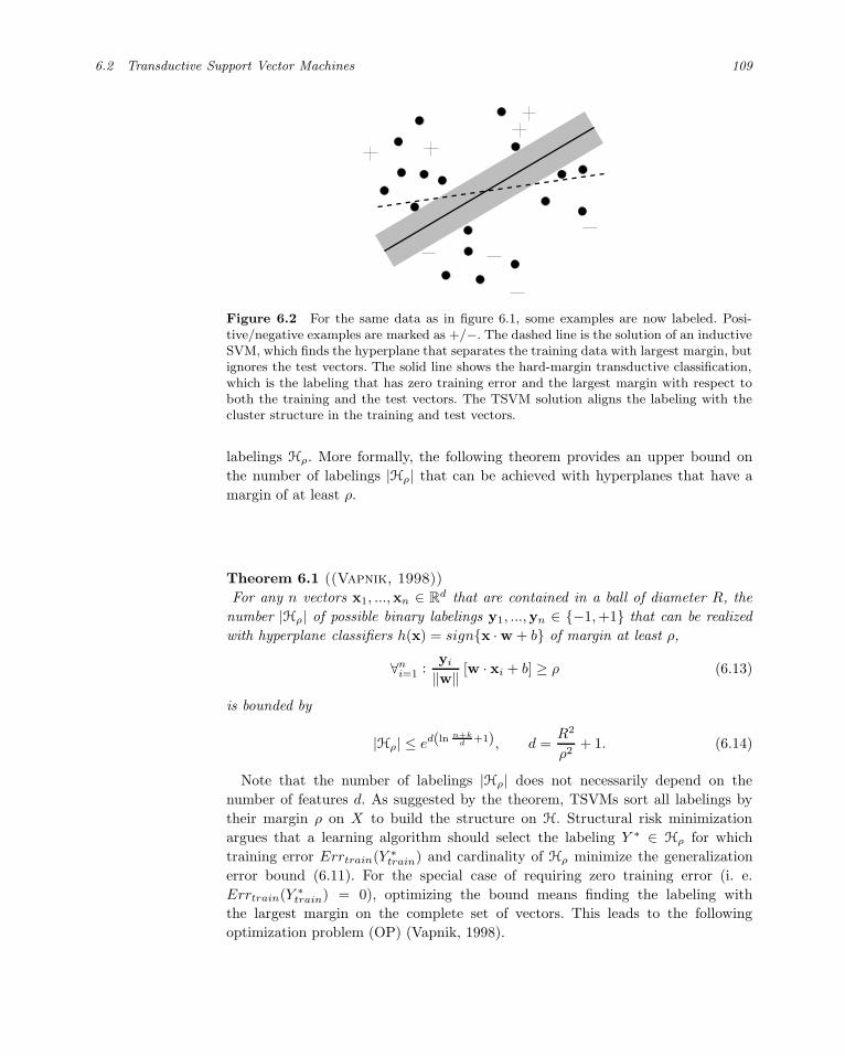
6.2 Transductive Support Vector Machines 109
Figure 6.2 For the same data as in figure 6.1, some examples are now labeled. Posi-tive/negative examples are marked as +/−. The dashed line is the solution of an inductiveSVM, which finds the hyperplane that separates the training data with largest margin, butignores the test vectors. The solid line shows the hard-margin transductive classification,which is the labeling that has zero training error and the largest margin with respect toboth the training and the test vectors. The TSVM solution aligns the labeling with thecluster structure in the training and test vectors.
labelings Hρ. More formally, the following theorem provides an upper bound on
the number of labelings |Hρ| that can be achieved with hyperplanes that have a
margin of at least ρ.
Theorem 6.1 ((Vapnik, 1998))
For any n vectors x1, ...,xn ∈ Rd that are contained in a ball of diameter R, the
number |Hρ| of possible binary labelings y1, ...,yn ∈ −1, +1 that can be realized
with hyperplane classifiers h(x) = signx · w + b of margin at least ρ,
∀ni=1 :
yi
‖w‖ [w · xi + b] ≥ ρ (6.13)
is bounded by
|Hρ| ≤ ed(ln n+kd
+1), d =R2
ρ2+ 1. (6.14)
Note that the number of labelings |Hρ| does not necessarily depend on the
number of features d. As suggested by the theorem, TSVMs sort all labelings by
their margin ρ on X to build the structure on H. Structural risk minimization
argues that a learning algorithm should select the labeling Y ∗ ∈ Hρ for which
training error Errtrain(Y ∗train) and cardinality of Hρ minimize the generalization
error bound (6.11). For the special case of requiring zero training error (i. e.
Errtrain(Y ∗train) = 0), optimizing the bound means finding the labeling with
the largest margin on the complete set of vectors. This leads to the following
optimization problem (OP) (Vapnik, 1998).

110 Transductive Support Vector Machines
OP1 (Transductive SVM (hard-margin))hard-margin
TSVMminimize: V (y∗
u1, ...,y∗
uu,w, b) =
1
2w ·w (6.15)
subject to: ∀li=1 : yli [w · xli + b] ≥ 1 (6.16)
∀uj=1 : y∗
uj[w · x∗
uj+ b] ≥ 1 (6.17)
∀uj=1 : y∗
uj∈ −1, +1 (6.18)
Solving this problem means finding the labeling y∗u1
, ...,y∗uk
of the test data for
which the hyperplane that separates both training and test data has maximum
margin. Figure 6.2 illustrates this. The figure also shows the solution that an
inductive SVM (Cortes and Vapnik, 1995; Vapnik, 1998) computes. An inductiveinductive SVM
SVM also finds a large-margin hyperplane, but it considers only the training
vectors while ignoring all test vectors. In particular, a hard-margin inductive SVM
computes the separating hyperplane that has zero training error and the largest
margin with respect to the training examples.
To be able to handle nonseparable data, one can introduce slack variables ξi
(Joachims, 1999) similar to inductive SVMs (Cortes and Vapnik, 1995).
OP2 (Transductive SVM (soft-margin))soft-margin
TSVM
min: W (y∗u1
, ...,y∗uu
,w, b, ξ1, ..., ξl, ξ∗1 , ..., ξ∗u)=
1
2w·w + C
l∑
i=1
ξi + C∗u∑
j=1
ξ∗j (6.19)
s.t.: ∀li=1 : yli [w · xli + b] ≥ 1 − ξi (6.20)
∀uj=1 : y∗
uj[w · x∗
uj+ b] ≥ 1 − ξ∗j (6.21)
∀uj=1 : y∗
uj∈ −1, +1 (6.22)
∀li=1 : ξi ≥ 0 (6.23)
∀uj=1 : ξ∗j ≥ 0 (6.24)
C and C∗ are parameters set by the user. They allow trading off margin size
against misclassifying training examples or excluding test examples. C∗ can be
used reduce sensitivity toward outliers (i.e., single examples falsely reducing the
margin on the test data).
Both inductive and transductive SVMs can be extended to include kernels (Boserkernels
et al., 1992; Vapnik, 1998). Making use of duality techniques from optimization
theory, kernels allow learning nonlinear rules as well as classification rules over
nonvectorial data (see e.g. (Scholkopf and Smola, 2002)) without substantially
changing the optimization problems.
Note that in both the hard-margin formulation (OP1) and the soft-margin formu-
lation (OP2) of the TSVM, the labels of the test examples enter as integer variables.
Due to the constraints in Eqs. 6.18 and 6.22 respectively, both OP1 and OP2 are
no longer convex quadratic programs like the analogous optimization problems for
inductive SVMs. Before discussing methods for (approximately) solving the TSVM

6.3 Why Use Margin on the Test Set? 111
salt andbasilparsleyatomphysicsnuclear
D1
D2
D3
D4
D5
D6
1 1
1
1
1
1 1
1 1
1
1
1
1
1
1
1
1
Figure 6.3 Example of a text-classification problem with co-occurrence pattern. Rowscorrespond to documents, columns to words. A table entry of 1 denotes the occurrence ofa word in a document.
optimization problems, let’s first discuss some intuition about why structuring the
hypothesis space based on the margin on the test examples might be reasonable.
6.3 Why Use Margin on the Test Set?
Why should it be reasonable to prefer a labeling with a large margin over a labeling
with a smaller margin, even if both have the same training error? Clearly, this
question can only be addressed in the context of a particular learning problem. In
the following, we will consider text classification as an example. In particular, for
topic-based text classification it is known that good classification rules typically
have a large margin (Joachims, 2002). The following example gives some intuition
for why this is the case.
In the field of information retrieval it is well known that words in natural language
occur in co-occurrence patterns (see e.g. (van Rijsbergen, 1977)). Some words are
likely to occur together in one document; others are not. For examples, when
asking Google about all documents containing the words pepper and salt, it
returns 3,500,000 webpages. When asking for the documents with the words pepper
and physics, we get only 248,000 hits, although physics (162,000,000 hits) is a
more popular word on the web than salt (63,200,000 hits). Many approaches in
information retrieval try to exploit this cluster structure of text (see e.g. (Baeza-
Yates and Ribeiro-Neto, 1999, chapter 5)). It is this co-occurrence information that
TSVMs exploit as prior knowledge about the learning task.
Consider the example in figure 6.3. Imagine document D1 was given as a training
example for class A and document D6 was given as a training example for class
B. How should we classify documents D2 to D5 (the test set)? Even if we did
not understand the meaning of the words, we would classify D2 and D3 into class
A, and D4 and D5 into class B. We would do so even though D1 and D3 do
not share any informative words. The reason we choose this classification of the
test data over the others stems from our prior knowledge about the properties of
text and common text-classification tasks. Often we want to classify documents by

112 Transductive Support Vector Machines
0
20
40
60
80
100
960348012400120064032617088462617
Ave
rag
e P
/R-b
rea
ke
ve
n p
oin
t
Number of Examples in training set
Transductive SVMSVM
Naive Bayes
Figure 6.4 Macro-averaged PRBEP on the Reuters data set for different training setsizes and a test set size of 3299.
topic, source, or style. For these types of classification tasks we find stronger co-
occurrence patterns within classes than between different classes. In our example
we analyzed the co-occurrence information in the test data and found two clusters.
These clusters indicate different topics of D1, D2, D3 versus D4, D5, D6, and
we choose the cluster separator as our classification. Note again that we got to this
classification by studying the location of the test examples, which is not possible
for an inductive learner.
The TSVM outputs the same classification as we suggested above, although all
16 labelings of D2 to D5 can be achieved with linear separators. Assigning D2
and D3 to class A and D4 and D5 to class B is the maximum-margin solution
(i.e., the solution of OP1). The maximum-margin bias appears to reflect our prior
knowledge about text classification well. By measuring margin on the test set, the
TSVM exploits co-occurrence patterns that indicate boundaries between topics.
6.4 Experiments and Applications of TSVMs
Structuring the hypothesis space using margin was obviously beneficial in the toy
example above. Experiments have confirmed that this also holds in practice.
Figures 6.4 and 6.5 (from Joachims (1999)) give empirical evidence thatTSVMs in text
classification TSVMs improve prediction performance on real text-classification tasks, namely
the Reuters-21578 text-classification benchmark. The standard “ModApte” train-
ing/test split is used, leading to a corpus of 9603 training documents and 3299
test documents. The results are averaged over the ten most frequent topics, while
keeping all documents. Each topic leads to a binary classification problem, where
documents about the topic are positive examples, and all other documents are neg-

6.4 Experiments and Applications of TSVMs 113
0
10
20
30
40
50
60
70
80
90
100
32991650825412206
Ave
rag
e P
/R-b
rea
ke
ve
n p
oin
t
Number of Examples in test set
Transductive SVMSVM
Naive Bayes
Figure 6.5 Macro-averaged PRBEP on the Reuters data set for 17 training documentsand varying test set size for the TSVM.
ative examples. The performance of each binary classifier is measured in terms of
the precision/recall breakeven point (PRBEP). The PRBEP is the percentage of
positive test examples that are classified correctly, if the classifier is allowed to pre-
dict as many test examples as positive as there are true positives in the test set
(see e.g. (Joachims, 2002)). The precise setup is described in (Joachims, 1999).
Figures 6.4 and 6.5 show the effect of using TSVM instead of inductive methods.
To provide a baseline for comparison, the results of the inductive SVM and a
multinomial naive Bayesnaive Bayes classifier are added. The SVM and the TSVM
are trained using SVMlight, available at svmlight.joachims.org. Figure 6.4 shows
the effect of varying the size of the training set. The advantage of using the
transductive approach is largest for small training sets. For increasing training
set size, the performance of the SVM approaches that of the TSVM. This is to be
expected, since labeled examples eventually convey the same information about the
distribution of the example vectors as the unlabeled data.
The influence of the test set size on the performance of the TSVM is displayed
in figure 6.5. The bigger the test set, the larger the performance gap between
SVM and TSVM. Adding more test examples beyond 3299 is not likely to increase
performance by much, since the graph appears to flatten out. The curves are fairly
typical and similar behavior was also observed on other problems. The results for
other text classification data sets can be found in (Joachims, 2002).
Similar gains in performance of the TSVM over an inductive SVM were reported
by Chapelle et al. (2003). For classifying net news articles they report that the
TSVM almost halves the prediction error for small training sets of 16 examples.
For an email classification problem, the results of Kockelkorn et al. (2003) also
indicate that TSVMs substantially outperform inductive SVMs for small training
sets. Small improvements on text classification problems are also reported by
Tong and Koller (2001). However, they conclude that the effect of active learning,

114 Transductive Support Vector Machines
where the algorithm can ask for the labels of particular examples, dominates the
improvement seen from the TSVM. This is in contrast to the findings of Wang et al.TSVMs for image
retrieval (2003). They find that incorporating TSVMs into their active learning procedure
for image retrieval based on relevance feedback substantially improves performance.
For more text-classification experiments see chapter 3.
Beyond text classification, Bennett and Demiriz (1999) have applied their L1-TSVMs for UCI
benchmarks norm variant of transductive SVMs to several UCI benchmark problems. They find
small but fairly consistent improvements over these tasks. A key difference from
most other experiments with transductive learning are the small test sets that
were used. Due to efficiency limitations of the mixed-integer programming code
they used for training, all test sets contained no more than 70 examples. Their
evaluation of regular TSVMs on a subset of these UCI benchmarks shows mixed
results (Demiriz and Bennett, 2000). Similar findings on UCI benchmarks are also
reported by Joachims (2003), where the differences between inductive SVMs and
TSVMs were found to be small.
Several applications of TSVMs in bioinformatics have been explored. For exam-TSVMs in
bioinformatics ple, they have been used to recognize promoter sequences in genes. Kasabov and
Pang (2004) report that TSVMs substantially outperform inductive SVMs in their
experiments. However, for the problem of predicting the functional properties of
proteins, Krogel and Scheffer (2004) find that TSVMs significantly decrease perfor-
mance compared to inductive SVMs.
Goutte et al. (2002) apply TSVMs to a problem of recognizing entities (e.g., geneTSVMs for
named entity
recognition
names, protein names) in medical text. They find that TSVMs substantially im-
prove performance for medium-sized training sets, and perform at least comparably
to an alternative transductive learning method based on Fisher kernels.
Summarizing the results, it appears that TSVMs are particularly well suited for
text classification and several other (typically high-dimensional) learning problems.
However, on some problems the TSVM performs roughly equivalently to an induc-
tive SVM, or sometimes even worse. This is to be expected, since it is likely that
structuring the hypothesis space according to margin size is inappropriate for some
applications. Furthermore, it is likely that the difficulty of finding the optimum of
the TSVM optimization problem has led to suboptimal results in some cases. We
discuss algorithms for solving the TSVM optimization problem next.
6.5 Solving the TSVM Optimization Problem
Both the hard soft-margin TSVM optimization problems can be written as mixed-
integer problems with a quadratic objective and linear constraints. Unfortunately,
currently no algorithm is known to efficiently find a globally optimal solution.
Vapnik and colleagues (Vapnik and Sterin, 1977; Wapnik and Tscherwonenkis,mixed-integer
programming 1979) proposed the use of branch-and-bound search to find the global optimium of
the TSVM optimization problem. Similarly, Bennett and Demiriz (1999) consider
standard mixed-integer programming software like CPLEX to solve a variant of

6.5 Solving the TSVM Optimization Problem 115
the TSVM optimization problem. To be able to use such software, they replace
the term w · w = ‖w‖22 in the objective with ‖w‖1 so that the objective becomes
linear. However, while both approaches produce globally optimal solutions, they
can solve only small problems with less than 100 test examples in reasonable time.
Unfortunately, figure 6.5 suggests that the biggest benefits of transductive learning
occur only for larger test sets.
The algorithm implemented in SVMlight does not necessarily produce a globallySVMlight
optimal solution, but can handle test sets with up to 100,000 examples in reasonable
time (Joachims, 1999, 2002). Most of the empirical results in the previous section
were produced using this algorithm. The algorithm performs a kind of coordinate-
descent local search starting from an initial labeling of the test examples derived
from an inductive SVM. The ratio of test examples that are classified as positive
(by adjusting the hyperplane threshold b) in this initial labeling is specified by the
user or estimated from the ratio of positive to negative examples in the training set.
This ratio is maintained throughout the optimization process to avoid degenerate
solutions that assign all test examples to the same class.2 In every step of the
local search, the algorithm selects two examples (one positive and one negative)
and swaps their labels. The way the examples are selected guarantees a strict
improvement of the objective function (i.e., the soft margin) in every such step.
In addition, the algorithm starts with a small value of C∗ and raises it throughout
the optimization process. This means that most ξ∗ are non-zero in the initial phase
of the search, resulting in a smoother objective function. Toward the end of the
search, incrementally increasing the value of C∗ toward the desired target value
makes the problem closer to the desired objective. A more detailed explanation of
the algorithm is given in (Joachims, 2002).
A related block coordinate descent method was proposed by Demiriz and Bennettgradient descent
(2000). The algorithm also alternates between changing the labels of the test exam-
ples and recomputing the margin. Differences compared to the SVMlightalgorithm
lie in the selection of the labels to change, the number of labels that are changed
in each iteration, and in the heuristics that are aimed to avoid local optima. A
similar algorithm for the L1-norm variant of the TSVM is described by Fung and
Mangasarian (2001).
De Bie and Cristianini (2004a) explore a convex approximation of the TSVMsemi-definite
relaxation optimization problem (also see chapter 7). They present a relaxation that takes the
form of a semi-definite program. While this program can be solved in polynomial
time, it becomes too inefficient for test sets with more than 100 examples. However,
assuming a low-rank structure of the test labels derived from a spectral decomposi-
tion technique, De Bie and Cristianini push the efficieny limit to several thousands
of test examples.
2. In text classification, assigning all test examples to the same class typically gives largermargins than any other labeling. Clearly, this is an undesirable solution and indicatesa problem with the TSVM approach. A method that does not exhibit this problem ispresented in Joachims (2003).

116 Transductive Support Vector Machines
6.6 Connection to Related Approaches
The difficulty in solving the TSVM optimization problem has led to much interestgraph cuts
in other formulations of transductive learning algorithms. The goal is to exploit the
same type of relationship between the geometry of the test examples — or unlabeled
examples more generally — and their labels, but that have computationally more
convenient properties. Graph partitioning approaches based on st-min-cuts (Blum
and Chawla, 2001) and spectral graph partitioning explicitly or implicitly pursued
this goal (Belkin and Niyogi, 2002; Chapelle et al., 2003; Joachims, 2003; Zhu
et al., 2003b) (see also chapters 11, 12, 13, 14, and 15). For example, the method
in (Joachims, 2003) is explicitly derived analogous to a TSVM as a transductive
version of the k-nearest neighbor classifier.
Ridge regression is a method closely related to regression SVMs. Chapelle et al.ridge regression
(1999) derive a tranductive variant of ridge regression. Since the class labels do
not need to be discrete for regression problems, they show that the solution of the
associated optimization problem can be computed efficiently.
Co-training (Blum and Mitchell, 1998) exploits two redundant representations ofco-training
a learning problem for semi-supervised learning. A connection to general trans-
ductive learning comes from the insight that co-training produces transductive
learning problems that have large margin (Joachims, 2003, 2002). In fact, TSVMs
and spectral partitioning methods appear to perform well on co-training problems
(Joachims, 2003).
Connecting to concepts of algorithmic randomness, Gammerman et al. (1998),confidence
estimation Vovk et al. (1999), and Saunders et al. (1999) presented approaches to estimating
the confidence of a prediction based on a transductive setting. A similar goal using
a Bayesian approach is pursued by Graepel et al. (2000). Since their primary aim
is not a reduced error rate in general, but a measure of confidence for a particular
prediction, they consider only test sets with exactly one example.
6.7 Summary and Conclusions
Transductive support vector machines exploit the geometric (cluster) structure in
the feature vectors of the test examples, which makes them a particular kind of
semi-supervised learning method. In particular, TSVMs find the labeling of the
test examples that maximizes margin jointly on the training and the test data.
Intuitively, this produces labeling of the test examples so that class boundaries
follow cluster boundaries. Empirical findings suggest that TSVMs are particularly
well suited for text classification and several other (typically high-dimensional)
learning problems, often showing large accuracy gains for small training sets and
large test sets. However, on some problems the TSVM performs roughly equivalently
to an inductive SVM, or sometimes even worse. Partially, failure on some tasks may
be due to the difficulty of finding the optimum of the TSVM optimization problem.

6.7 Summary and Conclusions 117
Finding the globally optimal solution is intractable for interestingly sized test sets.
Existing algorithms resort to local search or to relaxing the optimization problem.
More work is needed on tractable formulations and algorithms for transductive
learning, as well as a deeper theoretical and empirical understanding of its potential.


7 Semi-Supervised Learning Using Semi-
Definite Programming
Tijl De Bie [email protected]
Nello Cristianini [email protected]
We discuss the problem of support vector machine (SVM) transduction, which is a
combinatorial problem with exponential computational complexity in the number
of unlabeled samples. Different approaches to such combinatorial problems exist,
among which are exact integer programming approaches (only feasible for very small
sample sizes, e.g. (Bennett and Demiriz, 1999)) and local search heuristics starting
from a suitably chosen start value such as the approach explained in chapter 6,
transductive support vector machines, and introduced in (Joachims, 1999) (scalable
to large problem sizes, but sensitive to local optima).
In this chapter, we discuss an alternative approach introduced in (De Bie and
Cristianini, 2004a), which is based on a convex relaxation of the optimization
problem associated with support vector machine transduction. The result is a semi-
definite programming (SDP) problem which can be optimized in polynomial time,
the solution of which is an approximation of the optimal labeling as well as a bound
on the true optimum of the original transduction objective function. To further
decrease the computational complexity, we propose an approximation that allows
solving transduction problems of up to 1000 unlabeled samples.
Lastly, we extend the formulation to more general settings of semi-supervised
learning, where equivalence and inequivalence constraints are given on labels of
some of the samples.
7.1 Relaxing SVM Transduction
In transduction problems, we are provided with a set of labeled data points (training
set), as well as a set of unlabeled data points (test set). Our interest is to find
suitable labels for the second set, with no immediate ambition to make predictions

120 Semi-Supervised Learning Using Semi-Definite Programming
for yet unseen data points that may become available later on. The way the SVM
transduction problems handle this is by finding those test set labels for which, after
training an SVM on the combined training and test set, the margin on the full data
set is maximal. This involves optimizing over all labelings of the test set an integer
programming problem with exponential cost.
Primal Let us recall the primal soft-margin SVM problem (see e.g. (Cristianini
and Shawe-Taylor, 2000) and (Shawe-Taylor and Cristianini, 2004) for an introduc-
tion to SVMs and kernel methods):
minξi,w1
2wT w + C
l∑
i=1
ξi
s.t. yiwT xi ≥ 1 − ξi
ξi ≥ 0.
We omitted the bias term here, as we will do throughout the entire chapter. This is
not a problem, as argued in (Poggio et al., 2001). Only the labeled data points are
involved in this optimization problem. Then, the transductive SVM can be written
asprimal
transductive
SVM formulation minξi,w,Yu
1
2wT w + C
n∑
i=1
ξi
s.t. yiwT xi ≥ 1 − ξi
ξi ≥ 0
Yu ∈ −1, 1u, (7.1)
where we used the notation Yu = (yl+1, . . . yn) for the set of test set labels, a column
vector containing the labels for the test points, and n = l + u for the total number
of training and test points. It is the combinatorial constraint 7.1 that makes this
optimization problem very hard to solve exactly.
Dual Very often it is more interesting to focus on the dual problem, as it
allows us to use the kernel trick for nonlinear classification and for classification
of nonvectorial data. The standard soft-margin SVM problem is given by
maxαl2αT
l 1− αTl (Kl ⊙ YlY
Tl )αl
s.t. C ≥ αi ≥ 0,
where αl = (α1, . . . αl) is a column vector of dual variables αi, and Kl is the kernel
matrix for the training set. With ⊙, the element-wise matrix product is meant.
The optimum of this optimization problem is equal to the inverse square of the
margin (plus an additional cost term in the soft margin formulation). Hence, since
we want to maximize the margin, the dual formulation of the transductive SVM
can be written asdual transductive
SVM formulation
7.1 Relaxing SVM Transduction 121
minY maxα 2αT 1− αT (K ⊙ Y Y T )α
s.t. C ≥ αi ≥ 0
Y =
(Yl
Yu
)
Yu ∈ −1, 1u.
Here, α = (α1, . . . , αl, αl+1, . . . αn) is a vector containing the dual variables for
both the training and the test set, K is the complete kernel matrix, and Y is the
complete label vector. Without loss of generality, we assume that the first l rows
and columns of K correspond to training points, the last u to test points. Again, it
is the same combinatorial constraint that makes finding an exact solution infeasible
for reasonably sized problems.
Without affecting the solution, we slightly reformulate the optimization problem
by introducing the matrix variable Γ = Y Y T which we will refer to as the label
matrix. The dual formulation then becomeslabel matrix Γ
minΓ maxα 2αT 1− αT (K ⊙ Γ)α
s.t. C ≥ αi ≥ 0
Γ = Y Y T =
(YlY
Tl YlY
Tu
YuY Tl YuY T
u
)(7.2)
Yu ∈ −1, 1u. (7.3)
All constraints are now linear (matrix) inequalities, and the objective is linear in Γ
and concave in α. However, the problem is still an integer program due to constraint
7.3 and hence the overall problem is not convex.
7.1.1 Relaxation to an SDP Problem
We will write the label matrix Γ as a block matrix using the notation
Γ =
(Γll Γlu
Γul Γuu
)=
(YlY
Tl YlY
Tu
YuY Tl YuY T
u
).
Symmetry constraints such as Γuu = ΓTuu and Γlu = ΓT
ul are understood and we will
never mention them explicitly. Now, observe that any matrix of rank 1 with ones
on the diagonal can be written as an outer product of a vector with itself where
this vector only contains 1 and −1 as its elements. Thus, the following proposition
holds:
Proposition 7.1 We can reformulate the constraints (7.2) and (7.3) by the equiv-
122 Semi-Supervised Learning Using Semi-Definite Programming
alent set of constraints:
diag (Γ) = 1
rank (Γ) = 1
Γ =
(YlY
Tl Γlu
Γul Γuu
).
These constraints are linear in the parameters, except for the rank constraint, which
is clearly nonconvex (indeed, a convex combination of two matrices of rank 1 will
generally be of rank 2). To deal with this problem, in this chapter we propose to
relax the constraint set by extending the feasible region to a convex set over which
optimization can be accomplished in a reasonable computation time. To retain a
good performance, it should not be much larger than the nonconvex set specified
by the constraints above.
Note that the constraints imply that the matrix Γ is positive semi-definite (PSD).
So, we can add Γ 0 as an additional constraint without modifying the problem.
The relaxation then consists in simply dropping the rank constraint.1 The resulting
relaxed optimization problem is
minΓ maxα 2αT 1− αT (K ⊙ Γ)α
s.t. C ≥ αi ≥ 0
diag (Γ) = 1
Γ 0
Γ =
(YlY
Tl Γlu
Γul Γuu
).
Of course, the rank of the resulting optimal matrix Γ will not necessarily be equal
to 1 anymore, and its entries not equal to 1 and −1. However, we can see that each
entry of Γ will still lie in the interval [−1, 1]. Indeed, since all principal submatrices
of a PSD matrix have to be PSD as well, every 2× 2 principal submatrix has to be
PSD, which for a matrix containing ones on its diagonal can only be achieved for
off-diagonal elements in [−1, 1]. Furthermore:
1. Ideally, we should relax the constraints so as to extend the feasible region to just theconvex hull of the constraints, which is the smallest convex set containing the feasibleregion of the original problem. For a label matrix Y Y T with Y ∈ −1, 1n, this convexhull is referred to as the cut polytope. However, no efficient description of the cut polytope isknown. Hence, one has to resort to convex relaxations of the cut polytope itself, such as theelliptope, which is essentially the relaxation used in this chapter. Other relaxations of thecut polytope are known (such as the metric polytope), and they can be used alternativelyor in addition. Tighter relaxations tend to be computationally more challenging, though,and for brevity we will not consider these here. For more information we refer the readerto (Helmberg, 2000; Anjos, 2001).

7.1 Relaxing SVM Transduction 123
Theorem 7.2 The above optimization problem is convex. More specifically, it is an
SDP problem.
Proof By introducing the notation
f(Γ) = maxα 2αT 1− αT (K ⊙ Γ)α
s.t. C ≥ αi ≥ 0,
we can rewrite this optimization problem as
minΓ f(Γ)
s.t. diag (Γ) = 1
Γ 0
Γ =
(YlY
Tl Γlu
Γul Γuu
).
Let us first concentrate on f(Γ). For a given Γ 0, the objective is concave and
the constraints are all linear, i.e., we have a convex optimization problem. One can
easily verify Slater’s constraint qualification (the existence of a strictly feasible point
in the constraint set, see e.g. (Anjos, 2001)), showing that strong duality holds. Let
us now write the dual optimization problem by using Lagrange multipliers 2µ ≥ 0
and 2ν ≥ 0 for the inequality constraints C ≥ αi and αi ≥ 0 respectively (the
factor 2 in front of µ and ν is used for notational convenience). By invoking strong
duality, which states that the dual optimum is equal to the primal optimum, we
can now write f(Γ) as
f(Γ) = minµ,ν maxα 2αT (1− µ + ν) − αT (K ⊙ Γ)α + 2CµT 1
s.t. µ ≥ 0
ν ≥ 0.
We note in passing that the optimal value for 1 − µ + ν will be orthogonal
to the null space of K ⊙ Γ, since otherwise the solution could grow to infinity
by increasing the component of α along this null space. Now, the maximization
with respect to α can be carried out explicitly: the optimum is reached for
α = (K ⊙Γ)†(1−µ+ν)+α0, where α0 is a term in the null space of K ⊙Γ. Here† is used to denote the Moore-Penrose inverse. Plugging this in gives
f(Γ) = minµ,ν (1 − µ + ν)T (K ⊙ Γ)†(1 − µ + ν) + 2CµT 1
s.t. µ ≥ 0
ν ≥ 0.

124 Semi-Supervised Learning Using Semi-Definite Programming
Note that α0 has vanished. After introducing an additional variable t,
f(Γ) = minµ,ν,t t
s.t. µ ≥ 0
ν ≥ 0
t ≥ (1 − µ + ν)T (K ⊙ Γ)†(1− µ + ν) + 2CµT 1.
Using the extended Schur complement lemma (see appendix), we can rewrite the
latter constraint as
(K ⊙ Γ (1 − µ + ν)
(1 − µ + ν)T t − 2CµT 1
) 0,
which is a PSD constraint on a matrix that is a linear function of the variables. We
can thus rewrite the entire optimization problem as a linear optimization problem
subject to linear (matrix) inequalities:
minΓ,µ,ν,t t (7.4)
s.t. µ ≥ 0
ν ≥ 0
diag (Γ) = 1
Γ 0(K ⊙ Γ (1− µ + ν)
(1− µ + ν)T t − 2CµT 1
) 0
Γ =
(YlY
Tl Γlu
Γul Γuu
). (7.5)
This is a convex optimization problem that is solvable in polynomial time (see e.g.
(Nesterov and Nemirovsky, 1994; Vandenberghe and Boyd, 1996)).
7.1.2 Some Simplifications
We can simplify the problem using the following two propositions:
Proposition 7.3 The optimal value for Γ will be of the form
Γ =
(YlY
Tl Ylγ
Tu
γuY Tl Γuu
).
Proof From the extended Schur complement lemma it follows that the column
space of Γlu should be orthogonal to the null space of YlYTl . This can only be if
Γlu = YlγTu for some vector γu.

7.1 Relaxing SVM Transduction 125
Proposition 7.4 The constraint Γ 0 is equivalent with
(1 γT
u
γu Γuu
) 0.
Proof We use the fact that a principal submatrix of a PSD matrix is PSD as well
(Horn and Johnson, 1985). By taking a principal submatrix of Γ containing exactly
one row and the corresponding column among the first l, and all of the last u rows
and columns, we can see that Γ 0 implies
(1 γT
u
γu Γuu
) 0. On the other hand,
from
(1 γT
u
γu Γuu
) 0 we get
(Yl 0
0 I
)(1 γT
u
γu Γuu
)(Yl 0
0 I
)T
=
(YlY
Tl Ylγ
Tu
γuY Tl Γuu
)= Γ 0.
Thus, the final formulation of the relaxed SVM transduction problem is given by
minΓuu,γu,µ,ν,t t
s.t. µ ≥ 0
ν ≥ 0
diag (Γuu) = 1(1 γT
u
γu Γuu
) 0
⎛⎜⎜⎝
K ⊙(
YlYTl Ylγ
Tu
γuY Tl Γuu
)(1 − µ + ν)
(1 − µ + ν)T t − 2CµT 1
⎞⎟⎟⎠ 0.
Here we would like to point out that the equality constraint on the diagonal
can also be turned into an inequality constraint without affecting the solution:
diag (Γuu) ≤ 1. Indeed, if the diagonal were lower than 1, we could simply increase
it without affecting the constraints or increasing the objective. We will use this fact
later in this chapter.
Computational Complexity The total number of variables is equal to O(l +
u2), the number of linear inequality constraints being O(l + u), and we have an
SDP constraint of size O(l + u) and one of size O(u). This implies a worst-case
computational complexity of O((l + u2)2(l + u)2.5
)(see (Vandenberghe and Boyd,
1996) for a computational study of SDP problems).
7.1.3 Estimation of the Label Vector
As noted earlier, the optimal value for Γ may have a rank different from 1. So it
does not provide us with a direct estimate for the label vector Yu. However, the

126 Semi-Supervised Learning Using Semi-Definite Programming
previous section gives us a hint of what a suitable estimate for it can be: it is given
by simply one of the columns of Γ corresponding to a positively labeled training
point. In other words, we propose to take the (thresholded) vector γu as an estimate
for the optimal test label vector.
Other approaches are possible, such as taking the dominant eigenvector of Γ,
or using a randomized approach. For more information on such methods, see
(Helmberg, 2000).
7.1.4 A Bound on the Performance of the Transductive SVM
The minimum of a relaxed minimization problem is always smaller than the
minimum of the unrelaxed problem. Therefore, our method immediately provides
a lower bound on the squared inverse margin (plus a cost term for the soft-margin
formulation), and hence an upper bound on the (soft) margin that can be achieved.
On the other hand, the (soft) margin of the SVM trained on the training and test
set with estimated test labels provides us with a lower bound. If both bounds are
close to each other, we can be confident that the global optimum has been found.
7.2 An Approximation for Speedup
In most practical cases, the computational complexity of this relaxation is still too
high. In this section we present an approximation technique that will allow for a
considerable speedup of the method at the cost of a reasonable performance loss.
It is notable that this technique may have wider applicability to speed up convex
relaxations of combinatorial problems, such as for the max-cut problem (see e.g.
(Helmberg, 2000)).
7.2.1 The Subspace Trick
Let us assume for a moment that we can come up with a d-dimensional subspace
of Rn that contains the optimal label vector Y . We represent this subspace by
the columns of the matrix V ∈ Rn×d which form a basis for it. Then the optimal
label matrix Γ = Y Y T can be represented as Γ = VMVT , with M ∈ Rd×d, a
symmetric matrix of rank 1. Our relaxation of the rank constraint on Γ to an
SDP constraint then translates in an analogous relaxation on M. The resulting
optimization problem can be obtained by simply replacing all occurrences of Γ
with VMVT in Eqs. 7.4 and 7.5 and optimizing over M instead of over Γ:

7.2 An Approximation for Speedup 127
minM,µ,ν,t t
s.t. µ ≥ 0
ν ≥ 0
diag(VMVT
)= 1
M 0(K ⊙
(VMVT
)(1 − µ + ν)
(1 − µ + ν)T t − 2CµT 1
) 0.
7.2.2 Finding a Subspace Close to the Label Vector
In practice, it seems impossible to come up with exactly such a subspace V.
However, there are several techniques to approximate it, which are based on fast
eigenvalue problems (De Bie et al., 2004; Kamvar et al., 2003; Joachims, 2003). Here
we choose to use the method proposed in (De Bie et al., 2004), which is based on a
spectral relaxation of the normalized graph cut cost function (see e.g. (De Bie et al.,
2005) for an introduction to spectral clustering and other eigenvalue problems in
pattern recognition). Let us first briefly recapitulate the basic spectral clustering
method (without label constraints). Subsequently we will show how it is possible
to constrain the result to satisfy the training label information.
The basic spectral clustering problem is solved by the following generalized
eigenvalue problem:
(diag (K1) − K)v = λdiag (K1)v,
and the generalized eigenvectors belonging to the small eigenvalues capture the
cluster structure in the data (which means that a label vector corresponding to
a good clustering of the data is likely to be close to the space spanned by these
generalized eigenvectors).
In order to ensure that the given training label information is respected by this
solution, additional constraints should be imposed on v. This can be achieved
constructively by making use what we call the label constraint matrix L, defined
by
L =
⎛⎜⎜⎝
1l+ 1l+ 0
1l− −1l− 0
1u 0 I
⎞⎟⎟⎠ ,
where 1l+ and 1l− are vectors containing as many ones as there are positively and,
respectively, negatively, labeled training points, and 1u contains u ones. Using L,
we can constrain v to respect the training label information by parameterizing it

128 Semi-Supervised Learning Using Semi-Definite Programming
as v = Lz. Then the generalized eigenvalue problem to be solved is
L′((diag (K1) − K)Lz = λL′diag (K1)Lz, (7.6)
and the corresponding constrained solution is v = Lz. For more details about this
method we encourage the reader to consult (De Bie et al., 2004).
A good subspace to which the label vector is likely to be close is then spanned
by the vectors vi = Lzi with zi the generalized eigenvectors of (7.6) corresponding
to the d smallest eigenvalues (except for the one equal to zero). Hence, we can
construct a good matrix V by stacking these vi next to each other.
We are interested in solutions Γ = VMVT for which oppositely labeled training
points xi and xj have entries Γ(i, j) = Γ(j, i) = −Γ(i, i) = −Γ(j, j) in the
label matrix Γ. This could be ensured by imposing additional constraints on
our optimization problem. However, it is easy to see that it can be ensured
constructively as well, by ignoring the contribution of the constant column in L to
vi, the ith column of V (i.e., by equating the first entry of zi to 0 before computing
vi as vi = Lzi.
The constraint on the diagonal diag (Γ) = 1 will in general be infeasible when
using the subspace trick. However, as noted above, we can turn it into an inequality
constraint diag (Γ) ≤ 1 without fundamentally changing the problem. In fact, if the
dimensionality d (i.e., the number of columns) of V were equal to u, there would be
no difference between the optimal solutions obtained with or without the subspace
approximation, as then the entire feasible region of Γ is the same. The diagonal
would then be equal to 1, even if only an inequality constraint is specified.
Computational Complexity The number of constraints remains roughly the
same as in the unapproximated optimization problem. However, we potentially gain
a lot in terms of number of free variables, which is now O(d2 + n). Therefore, for
fixed d, the worst-case computational complexity is O(n4.5). The actual value for d
can be chosen as large as can be handled by the available computational resources.
7.3 General Semi-Supervised Learning Settings
Thus far we have discussed the transductive setting, which is just one of the semi-
supervised learning tasks described in chapter 1. We will briefly point out, however,
how the technology in this chapter can straightforwardly be extended to deal with
more general settings.
7.3.1 Equivalence and Inequivalence Label Constraints
As in (De Bie et al., 2004) and in chapter 5 of this book, we are able to handle
more general semi-supervised learning settings (see also (De Bie et al., 2003) and

7.4 Empirical Results 129
(Shental et al., 2004) where similar constraints are exploited for doing dimension-
ality reduction and in computing a Gaussian mixture model respectively). Imagine
the situation where we are given grouplets of points for which a label vector Yi is
specified. If we allow such grouplets to contain only one data point, we can assume
without loss of generality that each point belongs to exactly one grouplet. The label
vector Yi indicates which points within the grouplet are given to be in the same
class (an equivalence constraint), namely those with the same entry 1 or −1 in Yi,
and which ones are given to belong to opposite classes (when their entry in Yi is
different, an inequivalence constraint). In between different grouplets no informa-equivalence and
inequivalence
constraints
tion is given. This means that the overall sign of such a grouplet label vector Yi is
arbitrary.
Then, using similar techniques as we used above, one can show that the label
matrix Γ should be a block matrix, with the diagonal blocks equal to YiYTi , and
the off-diagonal blocks (i, j) equal to γi,jYjYTi :
Γ =
⎛⎜⎜⎜⎜⎜⎝
Y1YT1 γ1,2Y1Y
T2 · · · γ1,kY1Y
Tk
γ2,1Y2YT1 Y2Y
T2 · · · γ2,kY2Y
Tk
......
. . ....
γk,1YkY T1 γk,2YkY T
2 · · · YkY Tk
⎞⎟⎟⎟⎟⎟⎠
.
where γi,j = γj,i are the variables over which we have to optimize. Clearly, the label
matrix as in the transduction scenario explained at the beginning of this chapter
is a special case thereof. Now we can also see that the sign of the label vectors Yi
is irrelevant: upon changing the sign of Yi; the optimal solution will simply change
accordingly by reversing the signs of γi,j and γj,i for all j.
We want to point out that this method makes it possible to tackle the transductive
SVM problem in a hierarchical way. First one can perform a crude clustering of the
data points into many small clusters (grouplets) that respect the training data.
Then, at a second stage, the semi-supervised SVM approach outlined above can be
employed. This may greatly reduce the computational cost of the overall algorithm.
7.3.2 The Subspace Trick
Also here the subspace trick can be applied in a very analogous way. Again we can
rely on the method described in (De Bie et al., 2004), which is also able to deal
with equivalence and inequivalence constraints.
7.4 Empirical Results
For all implementations we used SeDuMi, a general purpose primal-dual interior
point solver (Sturm, 1999) for Matlab. We only used the hard-margin SVM ver-

130 Semi-Supervised Learning Using Semi-Definite Programming
sions, which are obtained from the soft-margin formulations by equating µ to 0.
Comparisons with SVMlight (Joachims, 1999) are reported, with default parameter
settings.
7.4.1 The Basic SDP Relaxation
The kernel used in all experiments in this subection is the radial basis function
(RBF) kernel, and the width is set to the average over all data points of the distance
to their closest neighbor. Figure 7.1 shows an artificially constructed example of a
transduction problem solved by the basic SDP relaxation of the transductive SVM.
Only two data points were labeled, one for each of both classes. Clearly, a standard
inductive SVM would fail in this extreme case.
Furthermore, the transductive optimum is so far from the inductive optimum
that a greedy strategy such as SVMlight is bound to get stuck in a local optimum.
Indeed, the norm of the SVM weight vector at the optimal labeling found by the
SDP relaxation is 5.7, and for the SVMlight local optimum it is 7.3. Thus, the
labeling found by the SDP relaxation achieves a larger margin.2 Furthermore, it is
notable that the optimum of the relaxed optimization problem is 35.318608 while
the (inductive) SVM optimum when using the predicted labels for the unlabeled
data points is only slightly larger: 35.318613. This indicates that most likely the
optimal labeling has been found, since the optimal labeling of the SVM optimum
has to lie between these values (see section 7.1.4).
In figure 7.2 we show another artificial example, where the data seem to consist
of five clusters. We labeled six samples, at least one in each of the clusters. Both
the SDP relaxation and SVMlight clearly succeed in assigning the same label to
all data points that are within the same cluster, and consistent with the training
label in that cluster. Figure 7.3 shows the same data set with a different labeling
of the training points. The transductive optimum found by the SDP relaxation is
slightly imbalanced: 38 data points in one class, and 42 in the other. For this reason
SVMlight seems to classify two data points differently, as, by default, it tries to find
a solution with the same proportion of positively versus negatively labeled test
points as in the training set. The norm of the SVM weight vector for the optimal
labeling as found by the SDP relaxation is equal to 5.92, which is slightly smaller
than 5.96, the weight vector norm for the SVMlight solution. Hence also here the
SDP approach achieves a larger margin.
Again, in both cases the lower bound provided by the optimum of the SDP
relaxation supports the conclusion that the optimal labeling has been found. For
the first problem, the optimum of the SDP relaxation is 35.338, while the SVM
optimum for the predicted labels is 35.341. For the second problem, those optima
2. There is a catch in the comparison of both optima: the SDP method does not use anoffset parameter b, whereas SVMlight does include such an offset. The numbers reportedare the weight vector norms when including an offset, hence favoring SVMlight.

7.4 Empirical Results 131
1 0. 5 0 0.5 11
0. 8
0. 6
0. 4
0. 2
0
0.2
0.4
0.6
0.8
1
1 0. 5 0 0.5 11
0. 8
0. 6
0. 4
0. 2
0
0.2
0.4
0.6
0.8
1
Figure 7.1 The result of the basic SDP relaxation (left) and of SVMlight (right) on anartificially constructed transduction problem. The ’o’ and ’x’ signs represent the negativelyand positively labeled training points. The other data points are labeled by the algorithms.The contour lines are drawn for the SVM as trained on the complete set of data pointswith labels as determined by the transduction algorithms. The SDP relaxation yields thedesired result, while apparently SVMlight got stuck in a local optimum.
are 32.3934 and 32.3937 respectively.
7.4.2 The Subspace Approximation
We conducted a few experiments on the constitution data set used in (De Bie and
Cristianini, 2004c). This data set contains 780 articles, an equal number in German,
French, Italian, and English, that are translations of each other. Furthermore, the
articles are organized in so-called Titles. In our experiments, we solved two different
problems: one is the classification of English + French texts versus Italian + English
texts, and the other is the classification of the largest Title (roughly containing half
of all articles) versus the smaller Titles. We tested the SDP relaxation as well as
SVMlight on both problems for different training set sizes, and plot the results in
figure 7.4. The kernel used is the normalized bag of words kernel, and d = 4.
Apparently, SVMlight outperforms the approximated SDP relaxation on the
difficult problem of classifying articles according to the Title they belong to. This
is most likely due to the fact that the four-dimensional subspace is too small to
capture the fine cluster structure due to the different Titles. Only a subspace
dimensionality d larger than four would solve the problem. However, even though
the computational cost is polynomial in d, this quickly becomes computationally
demanding.
On the other hand, the approximated SDP relaxation outperforms an already
good performance of SVMlight for the easier problem, indicating that here the
spectral transduction method finds a subspace sufficiently close to the correct label
vector.

132 Semi-Supervised Learning Using Semi-Definite Programming
1 0. 5 0 0.5 11
0. 8
0. 6
0. 4
0. 2
0
0.2
0.4
0.6
0.8
1
1 0. 5 0 0.5 11
0. 8
0. 6
0. 4
0. 2
0
0.2
0.4
0.6
0.8
1
Figure 7.2 The result of the basic SDP relaxation on an artificially constructed trans-duction problem (left), and the result of SVMlight (right). Here we organized the datapoints in a few small clusters. In each of the clusters, one or two samples are labeled (intotal there are six training points). For both methods, the training label determines thetest labels of all data points within the cluster, as is desirable in most applications.
1 0. 5 0 0.5 11
0. 8
0. 6
0. 4
0. 2
0
0.2
0.4
0.6
0.8
1
1 0. 5 0 0.5 11
0. 8
0. 6
0. 4
0. 2
0
0.2
0.4
0.6
0.8
1
Figure 7.3 SDP transduction (left) and SVMlight (right) are applied to the same dataset as in figure 7.2, now with a different labeling of the training points. If we label thedata points according to the labeled point in the cluster they (visually) belong to, thistransduction problem is slightly unbalanced: one class of 38 points, the other of 42 points.Since SVMlight fixes the fraction of positively and negatively labeled data points to theirfraction in the training set (by default), two data points are split off the cluster left aboveto satisfy this constraint.

7.5 Summary and Outlook 133
0 0.2 0.4 0.6 0.8 10.5
0.55
0.6
0.65
0.7
0.75
0.8
0.85
0.9
0.95
1
Figure 7.4 The receiver operating characteristics (ROC) score evaluated on the testset, as a function of the size of the training set for both classification problems. Thebold lines are for the easy classification problem classifying languages, and the faintlines are for the harder classification problem classifying articles according to their“Title”. The performance of the approximated SDP relaxation is shown in solid lines,the SVMlight performance in dotted lines. Bars indicate the standard deviation over threerandomizations.
7.5 Summary and Outlook
In this chapter we have presented an alternative approach to the transductive SVM
as a combinatorial problem. Whereas early approaches to transduction are based on
learning a suitable metric (Cristianini et al., 2002b,a), and other methods tackled
the problem using exact integer programming approaches (Bennett and Demiriz,
1999) (with very limited scalability) or using a local search heuristic (Joachims,
1999), our approach consists of a relaxation of the combinatorial problem to a
convex optimization problem. More specifically, the resulting optimization problem
is an SDP, which can be solved in a worst-case polynomial time. The application
of SDP and other convex optimization techniques seems a very promising line of
current research in machine learning (see e.g. also (Lanckriet et al., 2004b,a)).
While the empirical results for the relaxation are generally better than with
SVMlight, unfortunately the scalability is still limited. To solve this problem, we
introduced an approximation technique of general applicability in relaxations of
combinatorial problems. The performance of this approximation strongly depends
on the quality of the approximation, and mixed empirical results in comparison
with SVMlight are reported.
Future work includes investigating whether the problem structure can be ex-
ploited to speed up the optimization problem. An important theoretical question

134 Semi-Supervised Learning Using Semi-Definite Programming
that remains unanswered is whether the relaxation allows finding a solution with a
margin that is provably within a fixed constant factor of the unrelaxed optimum.
As we pointed out, the relaxation does provide us with an interval within which
the true optimal solution must lie. However, the size of this interval is not known
a priori as is the case for, e.g., the relaxation of the max-cut problem (see e.g.
(Helmberg, 2000)). Lastly, it would be interesting to investigate theoretically what
the influence is of the subspace approximation on the optimum.
Appendix: The Extended Schur Complement Lemma
We state the Schur complement lemma without proof (see e.g. (Helmberg, 2000)):
Lemma 7.5 (Schur complement lemma) For symmetric matrices A ≻ 0 and
C 0:
C BT A−1B ⇔(
A B
BT C
) 0.
When the matrix A may be rank deficient, the following extended Schur comple-
ment lemma should be used. It is a generalization of the standard Schur complement
lemma. We provide it here with a proof:Extended Schur
complement
lemma Lemma 7.6 (Extended Schur complement lemma) For symmetric matrices
A 0 and C 0:
The column space of B ⊥ the null space of A
C BT A†B
⇔
(A B
BT C
) 0.
Proof We write the singular value decomposition (SVD) of A as
A =(
V V0
)( Λ 0
0 0
)(V V0
)T
= VΛVT ,
where V0 denotes the singular vectors for the null space of A, V the other singular
vectors, and Λ is a diagonal matrix containing the non-zero singular values of A,
i.e. Λ ≻ 0. The blocks are assumed to be compatible. Similarly, we write the SVD
of C as
C =(
W W0
)( ∆ 0
0 0
)(W W0
)T
= W∆WT .
(⇒) If the column space of B ⊥ V0, we can write B as B = VBV for some
matrix BV. Then also BT A†B = BTVΛ−1BV. So, from C BT A†B = BT
VΛ−1BV
and from Λ ≻ 0 and C 0, it follows from the Schur complement lemma that

7.5 Summary and Outlook 135
(Λ BV
BTV C
) 0. Left multiplication of both sides of this inequality with
(V 0
0 I
)and on the right with its transpose, yields
(A B
BT C
) 0.
(⇐) We will prove the orthogonality of the column space of B with the null space
of A by contradiction. So, assume that the column space of B is not orthogonal to
the null space V0 of A. Then, there exists a vector v0 in the span of V0 for which
BT v0 = b = 0. Now, we have that
(A B
BT C
)=
(VΛV B
BT C
) 0. Thus, for
any vector w, multiplying this matrix with
(v0
w
)on the right and on the left with
its transpose must result in a non-negative number: 2bT w + wT Cw ≥ 0. However,
plugging in w = −C†b−W0WT0 b yields 2bT w+wT Cw = −2bTW0W
T0 b−bT C†b <
0, and thus we reached a contradiction. So we have established that the column
space of B is orthogonal to the span of V0.
This means that we can write B as B = VBV for some particular BV, and
(A B
BT C
)=
(VΛVT VBV
BTVVT C
)=
(V 0
0 I
)(Λ BV
BTV C
)(V 0
0 I
)T
,
so that:(
A B
BT C
) 0 ⇒
(Λ BV
BTV C
) 0.
Since Λ ≻ 0 and C 0 we can invoke the Schur complement lemma, which
gives C BTVΛ−1BV 0. However from the orthonormality of singular vectors
VT V = I, and thus BTVΛ−1BV = BT
VVT VΛ−1VT VBV = BT A†B, meaning that
BT A†B 0.


8 Gaussian Processes and the Null-Category
Noise Model
Neil D. Lawrence [email protected]
Michael I. Jordan [email protected]
Gaussian process classifiers (GPCs) aim to predict the posterior probability of
the class label yi given a covariate vector xi. Under the standard assumptions
generally invoked by GPC practitioners, this posterior probability is unaffected
by unlabeled data points, providing no role for unlabeled data. This is in marked
contrast to margin-based methods such as the support vector machine (SVM);
for these methods the unlabeled data can influence the location of the decision
boundary, causing it to pass through regions of low data density (see chapter 6). In
this chapter we present an augmentation of the standard probabilistic classification
model which incorporates a null-category. Given a suitable probabilistic model
for the model category, we obtain a probabilistic counterpart of the margin. By
combining this noise model with a GPC we obtain a classification methodology
that is simultaneously discriminative, semi-supervised, and Bayesian. Our approach
incorporates the cluster assumption without explicitly modeling the data density
and without requiring specialized kernels.
8.1 Introduction
In this chapter we consider a Bayesian formulation of the classification problem and
propose a solution to the semi-supervised learning problem within the Bayesian
framework.
Bayesian methods are naturally used in the formulation of generative ap-
proaches to classification problems. Generative approaches explicitly model the
class-conditional densities p (xi|yi = 1) and p (xi|yi = −1), combining these densi-
ties with the class prior probabilities p (yi = 1) and p (yi = −1) and using the Bayes

138 Gaussian Processes and the Null-Category Noise Model
theorem to form posterior probabilities:
p (yi = 1|xi) =p (xi|yi = 1) p (yi = 1)∑
yip (xi|yi) p (yi)
.
In the semi-supervised setting in which a label yi is not observed, the corresponding
contribution to the likelihood is obtained by marginalizing over yi. This yields a
mixture density for xi, a contribution to the likelihood that is handled readily within
the Bayesian formulation as a standard missing-data problem. Thus semi-supervised
learning is easily accommodated within a generative Bayesian framework.
Generative methods have well-known limitations in terms of prediction perfor-
mance, however, and most of the recent literature on classification has been devoted
to the development of discriminative approaches. Many of the well-known exam-discriminative
classification ples of discriminative classifiers are non-Bayesian, including the support vector ma-
chine (SVM), kernelized logistic regression (KLR), and AdaBoost (Shawe-Taylor
and Cristianini, 2004). It is, however, also possible to develop discriminative clas-
sifiers within a Bayesian framework; in particular, Gaussian process classifiers are
discriminative classifiers that share with SVM and KLR the use of a kernel function
to form nonlinear discriminant boundaries in the input space (O’Hagan, 1992).
Bayesian approaches to discriminative classification focus on modeling the pos-
terior probability p (yi|xi). Naively, it would seem that semi-supervised learning is
simply not accommodated within any such approach—marginalizing over yi yields
a constant contribution to the likelihood, thus providing no information regarding
the parameters. Non-Bayesian approaches can skirt this difficulty. In particular,
statistical inference for a non-Bayesian classifier involves the specification of a “loss
function” (e.g., a margin-based loss function) in addition to the specification of the
model, and, as shown by several of the other chapters in this book, loss functions
can be concocted to capture information coming from unlabeled data points. A
related point is that non-Bayesian approaches need not model the posterior prob-
ability, and this provides additional flexibility in the design of the loss function.
Bayesian approaches, on the other hand, start with the posterior probability and
this appears to tie the hands of the designer, making it difficult, if not impossible,
to develop discriminative, semi-supervised Bayesian learners.
In this chapter we show that it is in fact possible to solve the semi-supervised
learning problem within a discriminative, Bayesian framework. To motivate the
basic idea, let us first be more precise regarding the naive intuition referred to above
by making use of graphical model representations of Bayesian classifiers. Considergraphical model
representation first the graphical model representation of a generative classifier, shown in the left
panel of figure 8.1. In this diagram θ parameterizes the class-conditional densities.
(We have omitted a node representing the class prior probabilities.) The rectangle,
or “plate,” captures replication. In particular, the diagram captures an assumption
that the data yi are independent and identically distributed, conditional on
xi and θ. Finally, shading represents conditioning; thus the graphical model in
figure 8.1 captures the standard supervised learning setting in which the labels yiare fully observed.

8.1 Introduction 139
Figure 8.1 (Left) The graphical representation of a generative model. (Right) Thegraphical representation of a discriminative model.
The right panel of figure 8.1 presents a graphical representation of a discrimina-
tive classifier. In this case θ parameterizes the posterior probability (the meaning
of θ is different in the two diagrams). Again the figure captures the standard su-
pervised learning setting.
Let us now consider the semi-supervised learning problem. In semi-supervised
learning the data X are split into a subset that is labeled, Xl, and a subset
that is unlabeled, Xu. This is captured in the graphical model representations
shown in figure 8.2. Consider the model shown in the left panel for the generative
case. Using the d-separation criterion for assessing conditional independence in
graphical models (Pearl, 1988), we see that the parameter θ and the class label yj
are dependent, by virtue of the fact that their common descendant xj is observed
(shaded in the graph). This graphical motif is often referred to as a “v-structure.”
When two nodes point to a common descendant they are (necessarily) independent
only when the descendant is unobserved. This holds true both when yj is observed
and when it is not. Thus both labeled and unlabeled data points will affect the
Bayesian posterior distribution for θ.
Figure 8.2 Graphical models for semi-supervised data in the generative framework (left)and the discriminative framework (right).
Contrast this with the situation in the discriminative model (right panel of

140 Gaussian Processes and the Null-Category Noise Model
figure 8.2). In this case the d-separation criterion shows that θ is independent of
xj for the unlabeled data. The observed value of xj will not have an effect on the
posterior distribution of θ when yj is unobserved.
In the remaining sections of this chapter we will show how the discriminative
model can be augmented to allow it to handle unlabeled data.
8.1.1 Augmenting the Model
In figure 8.2 (right panel) we saw how, in the discriminative approach, an unlabeled
data point fails to influence the posterior for θ and thus the position of the decision
boundary. This is because the unlabeled points and the parameters become d-
separated (independent from one another) when the label yj is unobserved. To
restore the dependence we need to augment the model. This can be done by
introducing an additional variable zi that is a child of yj and is always observed. As
shown in figure 8.3 this breaks the d-separation of xj and θ and allows probabilistic
dependence to flow between these variables—even when yj is unobserved.
Figure 8.3 The augmented discriminative model. Even when yj is unobserved xj is nolonger d-separated from θ because they have a common descendant which is observed.Note that for labeled examples the parameters are d-separated from the indicator variablezj by the observation of yj .
As a simple (and naive) example of such an augmented model, let zj be an
indicator variable that identifies whether or not the data point is labeled; i.e., zj isobservability
indicator taken to be 0 if the ith point is labeled and 1 if the point is unlabeled. Certainly zj
is itself always observed. Now by allowing the probability of a point being labeled to
depend on its label yi — i.e., by a particular specification of the model probability
p (zi|yi) — we can reintroduce the dependence of the parameters on the unlabeled
data.
Of course this simple device does not solve the semi-supervised learning problem.
Indeed, if we have no reason to believe that the probability of a data point being un-

8.2 The Noise Model 141
labeled is different in the two classes; i.e., if p (zj = 1|yj = 1) = p (zj = 1|yj = −1),
then we have p (zj) = p (zj |yj) and zj is effectively decoupled from yj, once again
d-separating θ from xj .
On the other hand, there is no need to restrict ourselves to binary indicator
variables; we can be more clever about the augmentation. The remainder of the
chapter develops the specific augmentation that we propose. As will be seen, our
proposal is similar in spirit to the transductive SVM (see chapter 6); we want to
place the decision boundary in a region of low data density. The assumption that
the interclass regions have lower data density is known as the cluster assumption
(see chapter 1). We will show how an augmented model can capture the spirit of
the cluster assumption—but without implementing an explicit density model.
8.2 The Noise Model
Our approach is based on the notion of a null-category, a class for which we never
observe any data. The null-category can be viewed as a probabilistic interpretation
of the “margin” in the SVM.1
To simplify our discussion of the null-category noise model, we first introduce
a latent process variable fi. This variable will allow us to discuss the noise model
independently of the “process model.” The latent variable allows the probability of
class membership to decompose as
p (yi|xi) =
∫p (yi|fi) p (fi|xi) dfi,
where we refer to p (yi|fi) as the noise model and p (fi|xi) as the process model.
8.2.1 Ordered Categorical Models
The null-category noise model derives from the general class of ordered categorical
models (Agresti, 2002). In the specific context of binary classification we will
consider an ordered categorical model containing three categories:
p (yi|fi) =
⎧⎪⎪⎨
⎪⎪⎩
φ(−(fi + a
2
))for yi = −1
φ(fi + a
2
)− φ
(fi − a
2
)for yi = 0
φ(fi − a
2
)for yi = 1
,
where φ (x) =∫ x
−∞ N (z|0, 1)dz is the cumulative Gaussian distribution function
and a is a parameter giving the width of category yi = 0 (see figure 8.4).
1. We are not the first to consider a probabilistic interpretation of the SVM loss function.Sollich (1999, 2000) treats the margin in terms of a “not sure” class, but this interpretationsuffers from problems of normalization.

142 Gaussian Processes and the Null-Category Noise Model
Figure 8.4 The ordered categorical noise model. The plot shows p (yi|fi) for differentvalues of yi. Here we have assumed three categories.
We can also express this model in an equivalent and simpler form by replacing
the cumulative Gaussian distribution by a Heaviside step function,
H(x) =
0 if x < 0
1 if x > 0,
and adding independent Gaussian noise to the process model:
p (yi|fi) =
⎧⎪⎪⎨
⎪⎪⎩
H(−(fi + 1
2
))for yi = −1
H(fi + 1
2
)− H
(fi − 1
2
)for yi = 0
H(fi − 1
2
)for yi = 1
,
where we have standardized the width parameter to 1, by assuming that the overall
scale is also handled by the process model.
8.2.2 The Null-Category Noise Model
As stated previously, to induce a statistical dependence between the unlabeled data
point, xi, and the parameters, θ, we can augment the model with an additional
variable zi which indicates whether the label is missing. For the null-category noise
model we also impose the constraint that
p (zi = 1|yi = 0) = 0; (8.1)
in other words, a data point cannot be from the category yi = 0 and be unlabeled.
We then parameterize the probabilities of missing labels for the other classes as
p (zi = 1|yi = 1) = γ+ and p (zi = 1|yi = −1) = γ−.
For points where the label is present the latent process is updated as usual
(because zi is d-separated from θ by yi). When the data point’s label is missing,

8.3 Process Model and Effect of the Null-Category 143
the posterior process is updated using the likelihood
p (zi = 1|fi) =∑
yi
p (yi|fi) p (zi = 1|yi) .
By marginalizing across yi when the label is missing and otherwise using the
standard likelihood, we recover the “effective likelihood function” for a single dataeffective
likelihood
function
point, L (fi). It takes one of three forms:
L (fi) =
⎧⎪⎪⎨
⎪⎪⎩
H(−(fi + 1
2
))for yi = −1, zi = 0
γ−H(−(fi + 1
2
))+ γ+H
(fi − 1
2
)for zi = 1
H(fi − 1
2
)for yi = 1, zi = 0
.
The constraint imposed by (8.1) implies that an unlabeled data point never
comes from the class yi = 0. Since yi = 0 lies between the labeled classes this
is equivalent to a hard assumption that no data come from the region around
the decision boundary. We can also soften this hard assumption, if so desired, by
injection of noise into the process model. If we also assume that our labeled data
only come from the classes yi = 1 and yi = −1 we will never obtain any evidence
for data with yi = 0; for this reason we refer to this category as the null-category
and the overall model as a null-category noise model (NCNM).
8.3 Process Model and Effect of the Null-Category
The noise model we have described can be used within a range of optimization
frameworks. Indeed, viewing the noise model as a probabilistic interpretation of
the SVM’s margin, if we specify
fi = wTxi,
prescribe a Gaussian prior distribution for w,
p (w) = N (w|0, I) ,
and let z have a multivariate Gaussian distribution with mean m and covariance
Σ,
N (z|m, Σ) =1
(2π)d2 |Σ| 12
exp
(−1
2(z − m)
TΣ−1 (z − m)
),
then the maximum a posteriori (MAP) solution for w is given by the linear SVMSVM as MAP
solution algorithm. Naturally fi can then be “kernelized” and the MAP solution for the
model becomes equivalent to the nonlinear SVM. However, in this domain the
meaning of a prior distribution over w is not entirely clear, and it is generally more
convenient to consider a process prior over fi. As is well known, the process prior

144 Gaussian Processes and the Null-Category Noise Model
which leads to the SVM as a MAP solution is the Gaussian process prior (for two
useful reviews of Gaussian processes see O’Hagan (1992); Williams (1998)). Under
the Gaussian process prior the values fi are jointly distributed as a zero-mean
Gaussian distribution with covariance given by the kernel matrix K.
8.3.1 Gaussian Processes
In the remainder of this chapter we will consider the use of a Gaussian process prior
over fi. The algorithms we consider update the process posterior in a sequential
manner, incorporating a single data point at a time. It is therefore sufficient to
consider a univariate distribution over fi given xi, of the form
p (fi|xi) = N (fi|μ (xi) , ς (xi)) ,
where the mean μ (xi) and the variance ς (xi) are functions of the covariate xi.
A natural consideration in this setting is the effect of our likelihood function on
the distribution over fi when incorporating a new data point. As we have already
mentioned, if we observe yi, then the parameters are d-separated from zi. In this
case the effect of the likelihood on the posterior process will be similar to thateffect on
posterior incurred in binary classification, in that the posterior will be a convolution of the
step function and a Gaussian distribution. However, when the data point’s label is
missing the effect will depend on the mean and variance of p (fi|xi). If this Gaussian
has little mass in the null-category region (i.e., the region between the classes), the
posterior will be similar to the prior. However, if the Gaussian has significant mass
in the null-category region, the outcome may be loosely described in two ways:
1. If p (fi|xi) “spans the likelihood,” figure 8.5 (left), then the mass of the posterior
can be apportioned to either side of the null-category region, leading to a bimodal
posterior. The variance of the posterior will be greater than the variance of the prior,
a consequence of the fact that the effective likelihood function is not log-concave
(as can be easily verified).
2. If p (fi|xi) is “rectified by the likelihood,” figure 8.5 (right), then the mass of the
posterior will be pushed into one side of the null-category and the variance of the
posterior will be smaller than the variance of the prior.
Note that for all situations in which a portion of the mass of the prior distribution
falls within the null-category region it is pushed out to one side or both sides. The
intuition behind the two situations is that in case 1, it is not clear what label the
data point has, but it is clear that it shouldn’t be where it currently is (in the
null-category). The result is that the process variance increases. In case 2 the data
point is being assigned a label and the decision boundary is pushed to one side of
the point so that it is classified according to the assigned label.
In figure 8.6, we demonstrate the effect of the null-category. We sampled a vector
(fi)500i=1 from a Gaussian process with an radial basis function (RBF) kernel. The
covariates (xi)500i=1 were sampled uniformly from the two-dimensional unit square.

8.4 Posterior Inference and Prediction 145
Figure 8.5 Two situations of interest. Diagrams show the prior distribution over fi
(long dashes), the effective likelihood function from the noise model when zi = 1 (shortdashes), and a schematic of the resulting posterior over fi (solid line). (Left) The posterioris bimodal and has a larger variance than the prior. (Right) The posterior has one dominantmode and a lower variance than the prior. In both cases the process is pushed away fromthe null-category.
0 0.2 0.4 0.6 0.8 10
0.2
0.4
0.6
0.8
1
0 0.2 0.4 0.6 0.8 10
0.2
0.4
0.6
0.8
1
Figure 8.6 Samples from a standard Gaussian process classifier with a probit noisemodel (left) and a Gaussian process with the null-category noise model (right). Thecovariate vectors were originally sampled uniformly from the unit square. The null-category noise model has the effect of reducing the data density in the region of thedecision boundary.
In the left panel, points were assigned to the class of yi = 1 with probability
φ (fi) and were otherwise assigned a class of yi = −1. In the right panel they were
assigned the class yi = 1 with probability φ(fi − 1
2
)and the class yi = −1 with
probability φ(−fi − 1
2
); all other points were assumed to have come from the null
category and were removed. Note that this rejection of points has the effect of
reducing the data density near the decision boundary.
8.4 Posterior Inference and Prediction
Broadly speaking, the effects discussed above are independent of the process model:
the effective likelihood will always force the latent function away from the null-

146 Gaussian Processes and the Null-Category Noise Model
category. To implement our model, however, we must choose a specific process model
and inference method. The nature of the noise model means that it is unlikely that
we will find a nontrivial process model for which inference (in terms of marginalizing
fi) will be tractable. We therefore turn to approximations which are inspired by
“assumed density filtering” (ADF) methods; see, e.g., Csato (2002). The idea in
ADF is to approximate the (generally non-Gaussian) posterior with a Gaussian by
matching the moments between the approximation and the true posterior. ADF
has also been extended to allow each approximation to be revisited and improved
as the posterior distribution evolves (Minka, 2001).
One further complication is that the “effective likelihood” associated with the
null-category noise model is not log-concave. The implication of this is that the
variance of the posterior process can increase when a point is included. This
situation is depicted in figure 8.5 (left); the posterior depicted in this plot has
a larger variance than the prior distribution. This increase in variance is difficult to
accommodate within the ADF approximation framework and in our implementation
it was ignored.
One important advantage of the Gaussian process framework is that it is
amenable to an empirical Bayesian treatment—the hyperparameters in the covari-learning the
hyperparameters ance function can be learned by optimizing the marginal likelihood. In practice,
however, if the process variance is maximized in an unconstrained manner the ef-
fective width of the null-category can be driven to zero, yielding a model that is
equivalent to a standard binary classification noise model. The process variance
controls the scale of the function. If the process variance is allowed to grow in an
unconstrained manner the effective width of the null-category region becomes zero,
removing any effect from unlabeled data points. To prevent this from happening
we regularize by imposing an L1 penalty on the process variances (this is equiva-
lent to placing an exponential prior on those parameters). The L1 penalty prefers
smaller process variances thereby increasing the effective width of the null-category
region. The model therefore prefers a large null-category region. This is analogous
to maximizing the margin in a support vector machine.
8.4.1 Prediction with the NCNM
Once the parameters of the process model have been learned, we wish to make
predictions about a new test-point x∗ via the marginal distribution p (y∗|x∗). For
the NCNM an issue arises here: this distribution will have a non-zero probability of
y∗ = 0, a label that does not exist in either our labeled or unlabeled data. This is
where the role of z∗ becomes essential. The new point also has z∗ = 1 so in reality
the probability that a data point is from the positive class is given by
p (y∗|x∗, z∗ = 1) ∝ p (z∗ = 1|y∗) p (y∗|x∗) . (8.2)
The constraint that p (z∗ = 1|y∗ = 0) = 0 causes the predictions to be correctly
normalized. So for the distribution to be correctly normalized for a test data point

8.5 Results 147
we must assume that we have observed z∗ = 1.
An interesting consequence is that observing x∗ will have an effect on the process
model. This is contrary to the standard Gaussian process setup (see, e.g., Williams
(1998)) in which the predictive distribution depends only on the labeled training
data and the location of the test point x∗. In the NCNM the entire process model
p (f∗|x∗) should be updated after the observation of x∗. This is not a particular
disadvantage of the NCNM; it is an inevitable consequence of any method that
allows unlabeled data to affect the location of the decision boundary—a consequence
the probabilistic framework makes explicit. In practice, however, we may disregard
such considerations and make (possibly suboptimal) predictions of the class labels
according to (8.2) without updating the location of the decision boundary.
8.5 Results
Sparse representations of the training data are essential for speeding up the process
of learning. We made use of the informative vector machine (IVM) approach in
which the data are sparsified via a sequential greedy method in which points are
placed in an active set according to information-theoretic criteria. This approach
provides an approximation to a full Gaussian process classifier which is competitive
with the SVM in terms of speed and accuracy. The IVM also enables efficient
learning of kernel hyperparameters, and we made use of this feature in all of our
experiments.
10 5 0 5 1010
5
0
5
10
10 5 0 5 1010
5
0
5
10
Figure 8.7 Results from the toy problem. There are 400 points, which have probability0.1 of receiving a label. Labeled data points are shown as circles and crosses. Data pointsin the active set are shown as large dots. All other data points are shown as small dots.(Left) Learning on the labeled data with the IVM algorithm. All labeled points are usedin the active set. (Right) Learning on the labeled and unlabeled data with the NCNM.There are 100 points in the active set. In both plots decision boundaries are shown asa solid line; dotted lines represent contours within 0.5 of the decision boundary (for theNCNM this is the edge of the null-category).
148 Gaussian Processes and the Null-Category Noise Model
In all our experiments we used a kernel of the form
knm = θ2 exp(−θ1 (xn − xm)
T(xn − xm)
)+ θ3δnm,
where δnm is the Kronecker delta function. The parameters of the kernel were
learned by performing type II maximum likelihood over the active set. Since active
set selection causes the marginalized likelihood to fluctuate it cannot be used to
monitor convergence; we therefore simply iterated fifteen times between active set
selection and kernel parameter optimization. The parameters of the noise model,
γ+, γ−, can also be optimized, but note that if we constrain γ+ = γ− = γ, then
the likelihood is maximized by setting γ to the proportion of the training set that
is unlabeled.
We first considered an illustrative toy problem to demonstrate the capabilities
of our model. We generated two-dimensional data in which two class-conditional
densities interlock. There were 400 points in the original data set. Each point was
assigned a label with probability 0.1, leading to 37 labeled points. First a standard
IVM classifier was trained on the labeled data only (figure 8.7, left). We then used
the null-category approach to train a classifier that incorporates the unlabeled data.
As shown in figure 8.7 (right), the resulting decision boundary finds a region of low
data density and more accurately reflects the underlying data distribution.
8.5.1 USPS Digits
We next considered the null-category noise model for learning of the USPS hand-
written digit data set. This data set is fully labeled, but we can ignore a proportion
of the labels and treat the data set as a semi-supervised task. In the experiments
that followed we used an RBF kernel with a linear component. We ran each experi-
ment ten times, randomly selecting the data points that were labeled. The fraction
of labeled points, r, was varied between 0.01 and 0.25. Each digit was treated as a
separate “one against the others” binary classification class. We also summarized
these binary classification tasks with an overall error rate by allocating each test
data point to the class with the highest probability. In the first of our experiments,
we attempted to learn the parameters of the kernel by maximizing the IVM’s ap-
proximation to the marginal likelihood. The results are summarized in table 8.1.
As can be seen in the table, good classification results are obtained for values of
r above 0.1, but poor results are obtained for values of r below 0.1. This appears
troublesome at first sight, given that many semi-supervised learning algorithms give
reasonable performance even when the proportion of unlabeled data is as low as
0.1. It must be borne in mind, however, that the algorithm presented here faces the
additional burden of learning the kernel hyperparameters. Most other approaches
do not have this capability and therefore results are typically reported for a given,
tuned set of kernel parameters. To make a more direct comparison we also undertook
experiments in which the kernel hyperparameters were fixed to the values found by
an IVM trained on the fully labeled data set. These results are summarized in

8.6 Discussion 149
Table 8.1 Table of results for semi-supervised learning on the USPS digit data.
r 0 1 2 3 4
0.010 18 ± 0.0 8.0 ± 6.5 9.9 ± 0.0 8.3 ± 0.0 10 ± 0.0
0.025 11 ± 8.8 0.98 ± 0.1 9.9 ± 0.0 6.5 ± 2.4 10 ± 0.0
0.050 1.7 ± 0.2 1.0 ± 0.1 3.7 ± 0.4 5.4 ± 2.7 7.4 ± 3.5
0.10 1.7 ± 0.1 0.95 ± 0.1 3.2 ± 0.2 3.2 ± 0.3 3.3 ± 0.3
0.25 1.6 ± 0.2 0.97 ± 0.1 2.5 ± 0.2 2.9 ± 0.2 2.8 ± 0.1
r 5 6 7 8 9 Overall
0.010 8.0 ± 0.0 8.5 ± 0.0 7.3 ± 0.0 8.3 ± 0.0 8.8 ± 0.0 83 ± 7.3
0.025 8.0 ± 0.0 8.5 ± 0.0 7.3 ± 0.0 8.3 ± 0.0 8.8 ± 0.0 64 ± 5.0
0.05 7.1 ± 1.9 1.7 ± 0.2 7.3 ± 0.0 7.4 ± 1.9 7.6 ± 2.7 33 ± 7.2
0.1 3.0 ± 0.3 1.5 ± 0.1 1.3 ± 0.1 3.4 ± 0.2 2.0 ± 0.3 7.7 ± 0.2
0.25 2.4 ± 0.2 1.3 ± 0.2 1.2 ± 0.1 2.6 ± 0.3 1.6 ± 0.2 6.4 ± 0.2
For these results the model learned the kernel parameters. We give the results for the individualbinary classification tasks and the overall error computed from the combined classifiers. Eachresult is summarized by the mean and standard deviation of the percent classification error acrossten runs with different random seeds.
table 8.2. As expected these results are much better in the range where r < 0.1.
With the exception of the digit 2 at r = 0.01 a sensible decision boundary was
learned for at least one of the runs even when r = 0.01.
8.6 Discussion
We have presented a Bayesian approach to the semi-supervised learning problem.
While Bayesian approaches to semi-supervised learning are well known and easy to
formulate in the generative setting, they appear to be more difficult to formulate
in the discriminative setting—an unfortunate state of affairs given the superior
performance attainable with discriminative methods. Indeed, we are aware of no
previous work on classification algorithms that is simultaneously discriminative,
semi-supervised, and Bayesian. The approach presented in the previous paper shows
that this gap in the literature is not due to a fundamental limitation. Indeed,
discriminative, semi-supervised, Bayesian algorithms exist, and can be developed
via a relatively straightforward augmentation involving a “null-category.” Drawing
its inspiration from the role of the margin in the support vector machine, our null-
category noise model provides a probabilistic implementation of the assumption
that discriminant boundaries should pass through regions of low data density. We
achieve this within a fully discriminative framework that does not require modeling
of class-conditional densities.
Our approach provides a practical approach to performing kernel-based, semi-

150 Gaussian Processes and the Null-Category Noise Model
Table 8.2 Table of results for semi-supervised learning on the USPS digit data.
r 0 1 2 3 4
0.010 3.2 ± 5.2 13 ± 14 9.9 ± 0.0 3.1 ± 0.2 8.3 ± 2.6
0.025 1.5 ± 0.2 1.5 ± 0.9 5.2 ± 2.0 2.9 ± 0.2 4.4 ± 2.1
0.050 1.5 ± 0.2 1.2 ± 0.2 3.4 ± 0.4 2.9 ± 0.1 3.3 ± 0.2
0.10 1.5 ± 0.1 1.2 ± 0.1 2.8 ± 0.2 2.8 ± 0.2 3.0 ± 0.2
0.25 1.4 ± 0.2 1.3 ± 0.2 2.4 ± 0.2 2.6 ± 0.2 2.8 ± 0.2
r 5 6 7 8 9 Overall
0.010 7.5 ± 1.0 7.7 ± 8.5 12 ± 17 7.5 ± 1.2 35 ± 23 42 ± 10
0.025 5.0 ± 1.3 1.6 ± 0.2 1.9 ± 1.9 4.3 ± 0.5 9.9 ± 8.5 14 ± 6.1
0.050 3.6 ± 0.6 1.5 ± 0.1 1.3 ± 0.1 4.1 ± 0.4 2.6 ± 1.3 8.4 ± 0.7
0.10 2.8 ± 0.2 1.3 ± 0.1 1.3 ± 0.1 3.5 ± 0.3 2.0 ± 0.2 7.2 ± 0.5
0.25 2.3 ± 0.2 1.2 ± 0.1 1.2 ± 0.1 2.7 ± 0.2 1.6 ± 0.2 6.1 ± 0.4
For these results the model was given the kernel parameters learned by the IVM on the standardfully labeled data. We give the results for the individual binary classification tasks and the overallerror computed from the combined classifiers.
supervised learning without requiring the design of specialized kernels.
Code for recreating our experiments is available from http://www.dcs.shef.
ac.uk/~neil/ncnm.

9 Entropy Regularization
Yves Grandvalet [email protected]
Yoshua Bengio [email protected]
The problem of semi-supervised induction consists in learning a decision rule
from labeled and unlabeled data. This task can be undertaken by discriminative
methods, provided that learning criteria are adapted consequently. In this chapter,
we motivate the use of entropy regularization as a means to benefit from unlabeled
data in the framework of maximum a posteriori estimation. The learning criterion
is derived from clearly stated assumptions and can be applied to any smoothly
parameterized model of posterior probabilities. The regularization scheme favors
low-density separation, without any modeling of the density of input features. The
contribution of unlabeled data to the learning criterion induces local optima, but
this problem can be alleviated by deterministic annealing. For well-behaved models
of posterior probabilities, deterministic annealing expectation-maximization (EM)
provides a decomposition of the learning problem in a series of concave subproblems.
Other approaches to the semi-supervised problem are shown to be close relatives or
limiting cases of entropy regularization. A series of experiments illustrates the good
behavior of the algorithm in terms of performance and robustness with respect to
the violation of the postulated low-density separation assumption. The minimum
entropy solution benefits from unlabeled data and is able to challenge mixture
models and manifold learning in a number of situations.
9.1 Introduction
This chapter addresses semi-supervised induction, which refers to the learning of
a decision rule, on the entire input domain X, from labeled and unlabeled data.
The objective is identical to the one of supervised classification: generalize fromsemi-supervised
induction examples. The problem differs in the respect that the supervisor’s responses are
missing for some training examples. This characteristic is shared with transduction,
which has, however, a different goal, that is, of predicting labels on a set of

152 Entropy Regularization
predefined patterns.
In the probabilistic framework, semi-supervised induction is a missing data
problem, which can be addressed by generative methods such as mixture models
thanks to the EM algorithm and extensions thereof (McLachlan, 1992). Generative
models apply to the joint density of patterns x and class y. They have appealing
features, but they also have major drawbacks. First, the modeling effort is much
more demanding than for discriminative methods, since the model of p(x, y) is
necessarily more complex than the model of P (y|x). Being more precise, the
generative model is also more likely to be misspecified. Second, the fitness measure
is not discriminative, so that better models are not necessarily better predictors of
class labels. These issues are addressed in chapters 2 and 4.
These difficulties have led to proposals where unlabeled data are processed
by supervised classification algorithms. Here, we describe an estimation principle
applicable to any probabilistic classifier, aiming at making the most of unlabeled
data when they should be beneficial to the learning process, that is, when classes are
well apart. The method enables control of the contribution of unlabeled examples,
thus providing robustness with respect to the violation of the postulated low-density
separation assumption.
Section 9.2 motivates the estimation criterion. It is followed by the description
of the optimization algorithms in section 9.3. The connections with some other
principles or algorithms are then detailed in section 9.4. Finally, the experiments of
section 9.5 offer a test bed to evaluate the behavior of entropy regularization, with
comparisons to generative models and manifold learning.
9.2 Derivation of the Criterion
In this section, we first show that unlabeled data do not contribute to the maximum-
likelihood estimation of discriminative models. The belief that “unlabeled data
should be informative” should then be encoded as a prior to modify the estimation
process. We argue that assuming high entropy for P (y|x) is a sensible encoding
of this belief, and finally we describe the learning criterion derived from this
assumption.
9.2.1 Likelihood
The maximum-likelihood principle is one of the main estimation techniques in
supervised learning, which is closely related to the more recent margin maximization
techniques such as boosting and support vector machines (SVMs) (Friedman et al.,
2000). We start here by looking at the contribution of unlabeled examples to the
(conditional) likelihood.
The learning set is denoted Ln = (x1, y1), . . . , (xl, yl), xl+1, . . . , xn, where the
l first examples are labeled, and the u = n − l last ones are unlabeled. We
assume that labels are missing at random, that is, the missingness mechanismmissing value
mechanism

9.2 Derivation of the Criterion 153
is independent from the missing class information. Let h be the random variable
encoding missingness: h = 1 if y is hidden and h = 0 if y is observed. The missing
at random assumption readsmissing at
randomP (h|x, y) = P (h|x) . (9.1)
This assumption excludes cases where missingness may indicate a preference for a
particular class (this can happen, for example, in opinion polls where the “refuse
to answer” option may hide an inclination toward a shameful answer). Assuming
independent examples, the conditional log likelihood is then
L(θ; Ln) =
l∑
i=1
lnP (yi|xi; θ) +
n∑
i=1
lnP (hi|xi). (9.2)
Maximizing (9.2) with respect to θ can be performed by dropping the second
term of the right-hand side. It corresponds to maximizing the complete likelihood
when no assumption whatsoever is made on p(x) (McLachlan, 1992). As unlabeled
data are not processed by the model of posterior probabilities, they do not convey
information regarding P (y|x). In the maximum a posteriori (MAP) framework,
unlabeled data are useless regarding discrimination when the priors on p(x) and
P (y|x) factorize and are not tied (see chapter 2): observing x does not inform
about y, unless the modeler assumes so. Benefiting from unlabeled data requires
assumptions of some sort on the relationship between x and y. In the MAP
framework, this will be encoded by a prior distribution. As there is no such thing
as a universally relevant prior, we should look for an induction bias allowing the
processing of unlabeled data when the latter are known to convey information.
9.2.2 When Are Unlabeled Examples Informative?
Theory provides little support for the numerous experimental evidence showing
that unlabeled examples can help the learning process. Learning theory is mostly
developed at the two extremes of the statistical paradigm: in parametric statistics
where examples are known to be generated from a known class of distribution,
and in the distribution-free structural risk minimization (SRM) or probably ap-
proximately correct (PAC) frameworks. Semi-supervised induction does not fit the
distribution-free frameworks: no positive statement can be made without distribu-
tional assumptions, as for some distributions p(x, y), unlabeled data are noninfor-
mative while supervised learning is an easy task. In this regard, generalizing from
labeled and unlabeled data may differ from transductive inference.
In parametric statistics, theory has shown the benefit of unlabeled examples,
either for specific distributions (O’Neill, 1978), or for mixtures of the form p(x) =information
content of
unlabeled
examples
πp(x|y = 1)+(1−π)p(x|y = 2), where the estimation problem is essentially reduced
to the one of estimating the mixture parameter π (Castelli and Cover, 1996). These
studies conclude that the (asymptotic) information content of unlabeled examples
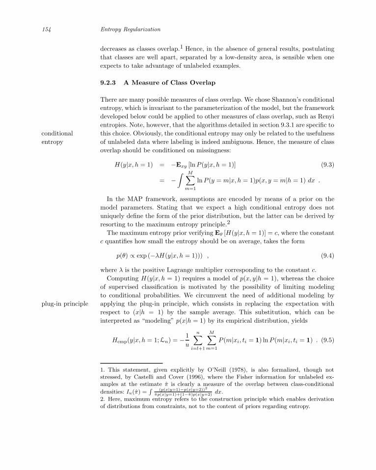
154 Entropy Regularization
decreases as classes overlap.1 Hence, in the absence of general results, postulating
that classes are well apart, separated by a low-density area, is sensible when one
expects to take advantage of unlabeled examples.
9.2.3 A Measure of Class Overlap
There are many possible measures of class overlap. We chose Shannon’s conditional
entropy, which is invariant to the parameterization of the model, but the framework
developed below could be applied to other measures of class overlap, such as Renyi
entropies. Note, however, that the algorithms detailed in section 9.3.1 are specific to
this choice. Obviously, the conditional entropy may only be related to the usefulnessconditional
entropy of unlabeled data where labeling is indeed ambiguous. Hence, the measure of class
overlap should be conditioned on missingness:
H(y|x, h = 1) = −Exy [lnP (y|x, h = 1)] (9.3)
= −∫ M∑
m=1
lnP (y = m|x, h = 1)p(x, y = m|h = 1) dx .
In the MAP framework, assumptions are encoded by means of a prior on the
model parameters. Stating that we expect a high conditional entropy does not
uniquely define the form of the prior distribution, but the latter can be derived by
resorting to the maximum entropy principle.2
The maximum entropy prior verifying Eθ [H(y|x, h = 1)] = c, where the constant
c quantifies how small the entropy should be on average, takes the form
p(θ) ∝ exp (−λH(y|x, h = 1))) , (9.4)
where λ is the positive Lagrange multiplier corresponding to the constant c.
Computing H(y|x, h = 1) requires a model of p(x, y|h = 1), whereas the choice
of supervised classification is motivated by the possibility of limiting modeling
to conditional probabilities. We circumvent the need of additional modeling by
applying the plug-in principle, which consists in replacing the expectation withplug-in principle
respect to (x|h = 1) by the sample average. This substitution, which can be
interpreted as “modeling” p(x|h = 1) by its empirical distribution, yields
Hemp(y|x, h = 1; Ln) = − 1
u
n∑
i=l+1
M∑
m=1
P (m|xi, ti = 1) lnP (m|xi, ti = 1) . (9.5)
1. This statement, given explicitly by O’Neill (1978), is also formalized, though notstressed, by Castelli and Cover (1996), where the Fisher information for unlabeled ex-amples at the estimate π is clearly a measure of the overlap between class-conditional
densities: Iu(π) =R (p(x|y=1)−p(x|y=2))2
πp(x|y=1)+(1−π)p(x|y=2)dx.
2. Here, maximum entropy refers to the construction principle which enables derivationof distributions from constraints, not to the content of priors regarding entropy.

9.3 Optimization Algorithms 155
The missing at random assumption (9.1) yields P (y|x, h = 1) = P (y|x), hence
Hemp(y|x, h = 1; Ln) = − 1
u
n∑
i=l+1
M∑
m=1
P (m|xi) lnP (m|xi) . (9.6)
This empirical functional is plugged in (9.4) to define an empirical prior on param-
eters θ, that is, a prior whose form is partly defined from data (Berger, 1985).
9.2.4 Entropy Regularization
The MAP estimate is defined as the maximizer of the posterior distribution, that
is, the maximizer of
C(θ, λ; Ln) = L(θ; Ln) − λHemp(y|x, h = 1; Ln)
=
l∑
i=1
lnP (yi|xi; θ) + λ
n∑
i=l+1
M∑
m=1
P (m|xi; θ) lnP (m|xi; θ) , (9.7)
where the constant terms in the log likelihood (9.2) and log prior (9.4) have been
dropped.
While L(θ; Ln) is only sensitive to labeled data, Hemp(y|x, h = 1; Ln) is only
affected by the value of P (m|x; θ) on unlabeled data. Since these two components of
the learning criterion are concave in P (m|x; θ), their weighted difference is usually
not concave, except for λ = 0. Hence, the optimization surface is expected to
possess local maxima, which are likely to be more numerous as u and λ grow. Semi-
supervised induction is halfway between classification and clustering; hence, the
progressive loss of concavity in the shift from supervised to unsupervised learning
is not surprising, as most clustering optimization problems are nonconvex (Rose
et al., 1990).
The empirical approximation Hemp (9.5) of H (9.3) breaks down for wiggly
functions P (m|·) with abrupt changes between data points (where p(x) is bounded
from below). As a result, it is important to constrain P (m|·) in order to enforce the
closeness of the two functionals. In the following experimental section, we imposed
such a constraint on P (m|·) by adding a smoothness penalty to the criterion C
(9.7). Note that this penalty also provides a means to control the capacity of the
classifier.
9.3 Optimization Algorithms
9.3.1 Deterministic Annealing EM and IRLS
In its application to semi-supervised learning, the EM algorithm is generally used
to maximize the joint likelihood from labeled and unlabeled data. This iterative
algorithm increases the likelihood at each step and converges toward a stationary

156 Entropy Regularization
point of the likelihood surface.
The criterion C(θ, λ; Ln) (9.7) departs from the conditional likelihood by its
entropy term. It is in fact formulated as each intermediate optimization subproblem
solved in the deterministic annealing EM algorithm. This scheme was originally
proposed to alleviate the difficulties raised by local maxima in joint likelihood
for some clustering problems (Rose et al., 1990; Yuille et al., 1994). It consistsdeterministic
annealing in optimizing the likelihood subject to a constraint on the level of randomness,
measured by the entropy of the model of P (y|x). The Lagrangian formulation of
this optimization problem is precisely (9.7), where T = 1 − λ is the analogue of a
temperature. Deterministic annealing is the cooling process defining the continuous
path of solutions indexed by the temperature. Following this path is expected to
lead to a final solution with lower free energy, that is, higher likelihood.
If the optimization criteria are identical, the goals, and the hyperparameters used
are different. On the one hand, in deterministic annealing EM, one aims at reaching
the global maximum (or at least a good local optimum) of the joint likelihood. For
this purpose, one starts from a concave function (T → ∞) and the temperature is
gradually lowered down to T = 1, in order to reach a state with high likelihood.
On the other hand, the goal of entropy regularization is to alter the maximum-
likelihood solution, by biasing it toward low entropy. One starts from a possibly
concave conditional likelihood (λ = 0, i.e., T = 1) and the temperature is gradually
lowered until it reaches some predetermined value 1 − λ0 = T0 ≥ 0, to return a
good local maximum of C(θ, λ0; Ln).
Despite these differences, the analogy with deterministic annealing EM is useful
because it provides an optimization algorithm for maximizing C(θ, λ; Ln) (9.7).
Deterministic annealing EM (Yuille et al., 1994) is a simple generalization ofdeterministic
annealing EM the standard EM algorithm. Starting from the solution obtained at the highest
temperature, the path of solution is computed by gradually increasing λ. For each
trial value of λ, the corresponding solution is computed by a two-step iterative
procedure, where the expected log likelihood is maximized at the M step, and
where soft (expected) assignments are imputed at the E step for unlabeled data.
The only difference with standard EM takes place at the E step, where the expected
value of labels is computed using the Gibbs distribution
gm(xi; θ) =P (m|xi; θ)
11−λ
∑Mℓ=1 P (ℓ|xi; θ)
11−λ
,
which distributes the probability mass according to the current estimated posterior
P (m|·) (for labeled examples, the assignment is clamped at the original label
gm(xi; θ) = δmyi). For 0 < λ ≤ 1, the Gibbs distribution is more peaked than
the estimated posterior. One recovers EM for λ = 0, and the hard assignments of
classification EM (CEM) (Celeux and Govaert, 1992) correspond to λ = 1.
The M step then consists in maximizing the expected log likelihood with respect

9.3 Optimization Algorithms 157
to θ,
θs+1 = argmaxθ
n∑
i=1
M∑
m=1
gm(xi; θs) lnP (m|xi; θ) , (9.8)
where the expectation is taken with respect to the distribution (g1(·; θs), . . . , gM (·; θs)),
and θs is the current estimate of θ.
The optimization problem (9.8) is concave in P (m|x; θ) and also in θ for logistic
regression models. Hence it can be solved by a second-order optimization algorithm,
such as the Newton-Raphson algorithm, which is often referred to as iteratively
reweighted least squares, or IRLS in statistical textbooks (Friedman et al., 2000).IRLS
We omit the detailed derivation of IRLS, and provide only the update equation
for θ in the standard logistic regression model for binary classification problems. 3
The model of posterior distribution is defined as
P (1|x; θ) =1
1 + e−(w⊤x+b), (9.9)
where θ = (w, b). In the binary classification problem, the M-step (9.8) reduces to
θs+1 = argmaxθ
n∑
i=1
g1(xi; θs) lnP (1|xi; θ) + (1− g1(xi; θ
s)) ln(1−P (1|xi; θ)) ,
where
g1(xi; θ) =P (1|xi; θ)
11−λ
P (1|xi; θ)1
1−λ + (1 − P (1|xi; θ))1
1−λ
for unlabeled data and g1(xi; θ) = δ1yifor labeled examples. Let pθ and g denote
the vector of P (1|xi; θ) and g1(xi; θs) values respectively, X the (n×(d+1)) matrix
of xi values concatenated with the vector 1, and Wθ the (n × n) diagonal matrix
with ith diagonal entry P (1|xi; θ)(1 − P (1|xi; θ)). The Newton-Raphson update is
θ ← θ +(X⊤WθX
)−1X⊤(g − pθ) . (9.10)
Each Newton-Raphson update can be interpreted as solving a weighted least squares
problem, and the scheme is iteratively reweighted by updating pθ (and hence Wθ)
and applying (9.10) until convergence.
9.3.2 Conjugate Gradient
Depending on how P (y|x) is modeled, the M step (9.8) may not be concave, and
other gradient-based optimization algorithms should be used. Even in the case
3. The generalization to kernelized logistic regression is straightforward, and the gener-alization to more than two classes results in similar expressions, but they would requirenumerous extra notations.

158 Entropy Regularization
where a logistic regression model is used, conjugate gradient may turn out being
computationally more efficient than the IRLS procedure. Indeed, even if each M step
of the deterministic annealing EM algorithm consists in solving a convex problem,
this problem is nonquadratic. IRLS solves exactly each quadratic subproblem, a
strategy which becomes computationally expensive for high-dimensional data or
kernelized logistic regression. The approximate solution provided by a few steps of
conjugate gradient may turn out to be more efficient, especially since the solution
θs+1 returned at the sth M step is not required to be accurate.
Depending on whether memory is an issue or not, conjugate gradient updates
may use the optimal steps computed from the Hessian, or approximations returned
by a line search. These alternatives have experimentally been shown to be much
more efficient than IRLS on large problems (Komarek and Moore, 2003).
Finally, when EM does not provide a useful decomposition of the learning task,
one can directly address the minimization of the learning criterion (9.7) with
conjugate gradient, or other gradient-based algorithms. Here also, it is useful to
define an annealing scheme, where λ is gradually increased from 0 to 1, in order to
avoid poor local maxima of the optimization surface.
9.4 Related Methods
9.4.1 Minimum Entropy in Pattern Recognition
Minimum entropy regularizers have been used in other contexts to encode learn-
ability priors (Brand, 1999). In a sense, Hemp can be seen as a poor man’s way to
generalize this approach to continuous input spaces. This empirical functional was
also used as a criterion to learn scale parameters in the context of transductive man-
ifold learning (Zhu et al., 2003b). During learning, discrepancies between H (9.3)
and Hemp (9.5) are prevented to avoid hard unstable solutions by smoothing the
estimate of posterior probabilities.
9.4.2 Input-Dependent and Information Regularization
Input-dependent regularization, introduced by Seeger (2000b) and detailed in chap-
ter 2, aims at incorporating some knowledge about the density p(x) in the modeling
of P (y|x). In the framework of Bayesian inference, this knowledge is encoded by
structural dependencies in the prior distributions.
Information regularization, introduced by Szummer and Jaakkola (2002a) and
extended as detailed in chapter 10, is another approach where the density p(x) is
assumed to be known, and where the mutual information between variables x and
y is penalized within predefined small neighborhoods. As the mutual information
I(x; y) is related to the conditional entropy by I(x; y) = H(y)−H(y|x), low entropy
and low mutual information are nearly opposite quantities. However, penalizing
mutual information locally, subject to the class constraints provided by labeled

9.4 Related Methods 159
examples, highly penalizes the variations of P (y|x) in the high-density regions.
Hence, like entropy regularization, information regularization favors solution where
label switching is restricted to low density areas between disagreeing labels.
Entropy regularization differs from these schemes in that it is expressed only in
terms of P (y|x) and does not involve a model of p(x). However, we stress that
for unlabeled data, the MAP minimum entropy estimation is consistent with the
maximum (complete)-likelihood approach when p(x) is small near the decision
surface. Indeed, whereas the complete likelihood maximizes ln p(x) on unlabeled
data, the regularizer minimizes the conditional entropy on the same points. Hence,
the two criteria agree provided the class assignments are confident in high-density
regions, or conversely, when label switching occurs in a low-density area.
9.4.3 Self-Training
Self-training is an iterative process, where a learner imputes the labels of examples
which have been classified with confidence in the previous step. This idea, which
predates EM, was independently proposed by several authors (see chapter 1). Amini
and Gallinari (2002) analyzed this technique and have shown that it is equivalent
to a version of the classification EM algorithm (Celeux and Govaert, 1992), which
minimizes the likelihood deprived of the entropy of the partition.
In the context of conditional likelihood estimation from labeled and unlabeled
examples, self-training minimizes C (9.7) with λ = 1. The optimization process itself
is identical to the generalized EM described in section 9.3.1 with hard assignments
(Grandvalet, 2002; Jin and Ghahramani, 2003).
Minimum entropy regularization is expected to have two benefits. First, the
influence of unlabeled examples can be controlled, in the spirit of EM-λ (Nigam
et al., 2000) Second, the deterministic annealing process, by which λ is slowly
increased, is expected to help the optimization process to avoid poor local minima of
the criterion. This scheme bears some similarity to the increase of the C∗ parameter
in the transductive SVM algorithm of Joachims (1999).
9.4.4 Maximal Margin Separators
Maximal margin separators are theoretically well-founded models which have shown
great success in supervised classification. For linearly separable data, they have been
shown to be a limiting case of probabilistic hyperplane separators (Tong and Koller,
2000).
In the framework of transductive learning, Vapnik (1998) proposed broaden-
ing the margin definition to unlabeled examples, by taking the smallest Euclidean
distance between any (labeled and unlabeled) training point to the classification
boundary. The following theorem, whose proof is given in the appendix, general-
izes theorem 5, corollary 6 of Tong and Koller (2000) to the margin defined in

160 Entropy Regularization
transductive learning4 when using the proposed minimum entropy criterion.
Theorem 9.1 Consider the two-class linear classification problem with linearly
separable labeled examples, where the classifier is obtained by optimizing
P (1|x; (w, b)) = 1/(1 + e−(w⊤x+b)) with the semi-supervised minimum entropy cri-
terion (9.7), under the constraint that ||w|| ≤ B. The margin of that linear classifier
converges toward the maximum possible margin among all such linear classifiers,
as the bound B goes to infinity.
Hence, the minimum entropy solution can approach semi-supervised SVM (Vap-
nik, 1998; Bennett and Demiriz, 1999). We, however, recall that the MAP criterion
is not concave in P (m|x; θ), so that the convergence toward the global maximum
cannot be guaranteed with the algorithms presented in section 9.3. This problem is
shared by all inductive semi-supervised algorithms dealing with a large number of
unlabeled data in reasonable time, such as mixture models or the transductive SVM
of Joachims (1999). Explicitly or implicitly, inductive semi-supervised algorithms
impute labels which are somehow consistent with the decision rule returned by the
learning algorithm. The enumeration of all possible configurations is only avoided
thanks to a heuristic process, such as deterministic annealing, which may fail.
Most graph-based transduction algorithms avoid this enumeration problem be-
cause their labeling process is not required to comply with a parameterized deci-
sion rule. This clear computational advantage has, however, its counterpart: label
propagation is performed via a user-defined similarity measure. The selection of
a discriminant similarity measure is thus left to the user, or to an outer loop, in
which case the overall optimization process is not convex anymore. The experimen-
tal section below illustrates that the choice of discriminant similarity measures is
difficult in high-dimensional spaces, and when a priori similar patterns should be
discriminated.
9.5 Experiments
9.5.1 Artificial Data
In this section, we chose a simple experimental setup in order to avoid artifacts
stemming from optimization problems. This setting enables checking to what
extent supervised learning can be improved by unlabeled examples, and when
minimum entropy can compete with generative methods which are traditionally
advocated in this framework. The minimum entropy criterion is applied to the
logistic regression model. It is compared to logistic regression fitted by maximum
likelihood (ignoring unlabeled data) and logistic regression with all labels known.
4. That is, the margin on an unlabeled example is defined as the absolute value of themargin on a labeled example at the same location.

9.5 Experiments 161
The former shows what has been gained by handling unlabeled data, and the latter
provides the “crystal ball” ultimate performance obtained by guessing correctly all
labels. All hyperparameters (weight-decay for all logistic regression models plus the
λ parameter (9.7) for minimum entropy) are tuned by tenfold cross-validation.
These discriminative methods are compared to generative models. Throughout
all experiments, a two-components Gaussian mixture model was fitted by the EM
algorithm (two means and one common covariance matrix estimated by maximum
likelihood on labeled and unlabeled examples (McLachlan, 1992)). The problem
of local maxima in the likelihood surface is artificially avoided by initializing
EM with the parameters of the true distribution when the latter is truly a two-
component Gaussian mixture, or with maximum likelihood parameters on the
(fully labeled) test sample when the distribution departs from the model. This
initialization advantages EM, which is guaranteed to pick, among all local maxima
of the likelihood, the one which is in the basin of attraction of the optimal
value. In particular, this initialization prevents interferences that may result from
the “pseudolabels” given to unlabeled examples at the first E step. The “label
switching” problem (badly labeled clusters) is prevented at this stage.
Correct Joint Density Model In the first series of experiments, we consider
two-class problems in a 50-dimensional input space. Each class is generated with
equal probability from a normal distribution. Class 1 is normal with mean (a a . . . a)
and unit covariance matrix. Class 2 is normal with mean −(a a . . . a) and unit
covariance matrix. Parameter a tunes the Bayes error which varies from 1 % to 20
% (1 %, 2.5 %, 5 %, 10 %, 20 %). The learning sets comprise l labeled examples,
(l = 50, 100, 200) and u unlabeled examples, (u = l× (1, 3, 10, 30, 100)). Overall, 75
different setups are evaluated, and for each one, ten different training samples are
generated. Generalization performances are estimated on a test set of size 10, 000.
This first benchmark provides a comparison for the algorithms in a situation
where unlabeled data are known to convey information. Besides the favorable
initialization of the EM algorithm to the optimal parameters, the generative models
benefit from the correctness of the model: data were generated according to the
model, that is, two Gaussian subpopulations with identical covariances. The logistic
regression model is only compatible with the joint distribution, which is a weaker
fulfillment than correctness.
As there is no modeling bias, differences in error rates are only due to differences
in estimation efficiency. The overall error rates (averaged over all settings) are in
favor of minimum entropy logistic regression (14.1 ± 0.3 %). EM (15.7 ± 0.3 %)
does worse on average than logistic regression (14.9 ± 0.3 %). For reference, the
average Bayes error rate is 7.7 % and logistic regression reaches 10.4± 0.1 % when
all examples are labeled.
Figure 9.1 provides more informative summaries than these raw numbers. The
first plot represents the error rates (averaged over l) versus the Bayes error rate
and the u/l ratio. The second plot represents the same performances on a common
scale along the abscissa, by showing the relative improvement of using unlabeled

162 Entropy Regularization
5 10 15 20
10
20
30
40
Bayes Error (%)
Tes
t E
rror
(%)
5 10 15 20
1
1.5
2
2.5
3
3.5
Bayes Error (%)
Rel
ativ
e im
pro
vem
ent
Figure 9.1 (Left): Test error of minimum entropy logistic regression () and mixturemodels (+) versus Bayes error rate for u/l = 10. The errors of logistic regression (dashed),and logistic regression with all labels known (dash-dotted) are shown for reference. (Right):Relative improvement to logistic regression versus Bayes error rate.
examples when compared to logistic regression ignoring unlabeled examples. The
relative improvement is defined here as the ratio of the gap between test error and
Bayes error for the considered method to the same gap for logistic regression. This
plot shows that, as asymptotic theory suggests (O’Neill, 1978; Castelli and Cover,
1996), unlabeled examples are more beneficial when the Bayes error is low. This
observation supports the relevance of the minimum entropy assumption.
Figure 9.2 illustrates the consequence of the demanding parametrization of gen-
erative models. Mixture models are outperformed by the simple logistic regression
model when the sample size is low, since their number of parameters grows quadrat-
ically (versus linearly) with the number of input features. This graph also shows
that the minimum entropy model takes quick advantage of unlabeled data when
classes are well separated. With u = 3l, the model considerably improves upon the
one discarding unlabeled data. At this stage, the generative models do not per-
form well, as the number of available examples is low compared to the number
of parameters in the model. However, for very large sample sizes, with 100 times
more unlabeled examples than labeled examples, the generative method eventually
becomes more accurate than the discriminative one.
These results are reminiscent of those of Efron (1975), in the respect that the
generative method is asymptotically slighly more efficient than the discriminative
one, mainly because logistic regression makes little use of examples far from the
decision surface. In the same respect, our observations differ from the comparison
of Ng and Jordan (2001), which shows that naive Bayes can be competitive in terms
of test error for small training sample sizes. This may be explained by the more
general generative model used here, which does not assume feature independance.
Misspecified Joint Density Model In a second series of experiments, the
setup is slightly modified by letting the class-conditional densities be corrupted by

9.5 Experiments 163
1 3 10 30 1005
10
15
Ratio u/l
Tes
t E
rro
r (%
)
Figure 9.2 Test error versus u/l ratio for 5 % Bayes error (a = 0.23). Test errors ofminimum entropy logistic regression () and mixture models (+). The errors of logisticregression (dashed), and logistic regression with all labels known (dash-dotted) are shownfor reference.
outliers. For each class, the examples are generated from a mixture of two Gaussians
centered on the same mean: a unit variance component gathers 98 % of examples,
while the remaining 2 % are generated from a large variance component, where
each variable has a standard deviation of 10. The mixture model used by EM is
now slightly misspecified since the whole distribution is still modeled by a simple
two-components Gaussian mixture. The results, displayed in the left-hand-side of
figure 9.3, should be compared with figure 9.2. The generative model dramatically
suffers from the misspecification and behaves worse than logistic regression for all
sample sizes. The unlabeled examples have first a beneficial effect on test error, then
have a detrimental effect when they overwhelm the number of labeled examples.
On the other hand, the discriminative models behave smoothly as in the previous
case, and the minimum entropy criterion performance steadily improves with the
addition of unlabeled examples.
The last series of experiments illustrate the robustness with respect to the
cluster assumption, by which the decision boundary should be placed in low-
density regions. The samples are drawn from a distribution such that unlabeled
data do not convey information, and where a low-density p(x) does not indicate
class separation. This distribution is modeled by two Gaussian clusters, as in the
first series of experiments, but labeling is now independent from clustering: example
xi belongs to class 1 if xi2 > xi1 and belongs to class 2 otherwise; the Bayes
decision boundary now separates each cluster in its middle. The mixture model is
unchanged. It is now far from the model used to generate data. The right-hand side
plot of figure 9.3 shows that the favorable initialization of EM does not prevent
the model from being fooled by unlabeled data: its test error steadily increases
with the amount of unlabeled data. Conversely, the discriminative models behave
well, and the minimum entropy algorithm is not distracted by the two clusters; its
performance is nearly identical to the one of training with labeled data only (cross-

164 Entropy Regularization
1 3 10 30 1005
10
15
20
Ratio u/l
Tes
t E
rror
(%)
1 3 10 30 1000
5
10
15
20
25
30
Ratio u/l
Tes
t E
rror
(%)
Figure 9.3 Test error versus u/l ratio for a = 0.23. Average test errors for minimumentropy logistic regression () and mixture models (+). The test error rates of logisticregression (dotted), and logistic regression with all labels known (dash-dotted) are shownfor reference. (Left): Experiment with outliers. (Right): Experiment with uninformativeunlabeled data.
Table 9.1 Error rates (%) of minimum entropy (ME) versus consistency method (CM),for a = 0.23, l = 50, and (a) pure Gaussian clusters, (b) Gaussian clusters corrupted byoutliers, and (c) class boundary separating one Gaussian cluster
nu 50 150 500 1500
a) ME 10.8 ± 1.5 9.8 ± 1.9 8.8 ± 2.0 8.3 ± 2.6
a) CM 21.4 ± 7.2 25.5 ± 8.1 29.6 ± 9.0 26.8 ± 7.2
b) ME 8.5 ± 0.9 8.3 ± 1.5 7.5 ± 1.5 6.6 ± 1.5
b) CM 22.0 ± 6.7 25.6 ± 7.4 29.8 ± 9.7 27.7 ± 6.8
c) ME 8.7 ± 0.8 8.3 ± 1.1 7.2 ± 1.0 7.2 ± 1.7
c) CM 51.6 ± 7.9 50.5 ± 4.0 49.3 ± 2.6 50.2 ± 2.2
validation provides λ values close to zero), which can be regarded as the ultimate
achievable performance in this situation.
Comparison with Manifold Transduction Although this chapter focuses on
inductive classification, we also provide comparisons with a transduction algorithm
relying on the manifold assumption. The consistency method (Zhou et al., 2004)
is a very simple label propagation algorithm with only two tuning parameters. As
suggested by Zhou et al. (2004), we set α = 0.99 and the scale parameter σ2 was
optimized on test results. The results are reported in table 9.1. The experiments
are limited due to the memory requirements of the consistency method in our naive
implementation.
The results are extremely poor for the consistency method, whose error is way

9.5 Experiments 165
Anger Fear Disgust Joy Sadness Surprise Neutral
Figure 9.4 Examples from the facial expression recognition database.
above minimum entropy, and which does not show any sign of improvement as the
sample of unlabeled data grows. In particular, when classes do not correspond to
clusters, the consistency method performs random class assignments.
In fact, the experimental setup, which was designed for the comparison of global
classifiers, is not favorable to manifold methods, since the input data are truly
50-dimensional. In this situation, finding a discriminant similarity measure may
require numerous degrees of freedom, and the consistency method provides only
one tuning parameter: the scale parameter σ2. Hence, these results illustrate that
manifold learning requires more tuning efforts for truly high-dimensional data, and
some recent techniques may respond to this need (Sindhwani et al., 2005).
9.5.2 Facial Expression Recognition
We now consider an image recognition problem, consisting in recognizing seven
(balanced) classes corresponding to the universal emotions (anger, fear, disgust,
joy, sadness, surprise, and neutral). The patterns are gray level images of frontal
faces, with standardized positions, as displayed in figure 9.4. The data set comprises
375 such pictures made of 140 × 100 pixels (Abboud et al., 2003; Kanade et al.,
2000)
We tested kernelized logistic regression (Gaussian kernel), its minimum entropy
version, nearest neighbor, and the consistency method. We repeatedly (10 times)
sampled 1/10 of the data set for providing the labeled part, and the remainder for
testing. Although (α, σ2) were chosen to minimize the test error, the consistency
method performed poorly with 63.8± 1.3 % test error (compared to 86 % error for
random assignments). Nearest neighbor gets similar results with 63.1 ± 1.3 % test
error, and kernelized logistic regression (ignoring unlabeled examples) improved
to reach 53.6 ± 1.3 %. Minimum entropy kernelized logistic regression regression
achieves 52.0 ± 1.9 % error (compared to about 20 % errors for human on this
database). The scale parameter chosen for kernelized logistic regression (by tenfold
cross-validation) amount to using a global classifier.
The failure of local methods may be explained by the fact that the database
contains several pictures of each person, with different facial expressions. Hence,
local methods are likely to pick the same identity instead of the same expression,
while global methods are able to learn the discriminating directions.

166 Entropy Regularization
9.6 Conclusion
Although discriminative methods do not benefit from unlabeled data in the
maximum-likelihoood framework, maximum a posteriori estimation enables ad-
dressing the semi-supervised induction problem. The information content of unla-
beled data decreases with class overlap, which can be measured by the conditional
entropy of labels given patterns. Hence, the minimum entropy prior encodes a
premise of semi-supervised induction, that is, the belief that unlabeled data may
be useful. The postulate is optimistic in some problems where unlabeled data do not
convey information regarding labels, but the strength of the prior is controlled by
a tuning parameter, so that the contribution of unlabeled examples to the estimate
may vanish.
Minimum entropy regularization is related to self-training in general and to
transductive SVMs in particular. It promotes classifiers with high confidence on
the unlabeled examples. A deterministic annealing process smoothly drives the
decision boundary away from unlabeled examples, favoring low-density separation.
The regularizer can be applied to local and global models of posterior probabili-
ties. As a result, it can improve over local models when they suffer from the curse of
dimensionality. Minimum entropy regularization may also be a serious contender for
generative methods. It compares favorably to these mixture models in three situa-
tions: for small sample sizes, where the generative model cannot completely benefit
from the knowledge of the correct joint model; when the joint distribution is (even
slightly) misspecified; when the unlabeled examples turn out to be noninformative
regarding class probabilities.
Finally, the algorithms presented in this chapter can be applied to a generalized
version of the semi-supervised induction problem, where the examples may be
labeled by any subset of labels, representing the set of plausible classes. This kind of
information is sometimes a more faithful description of the true state of knowledge
when labeling is performed by an expert.
Appendix: Proof of Theorem 9.1
Theorem 9.1 Consider the two-class linear classification problem with linearly sep-
arable labeled examples, where the classifier is obtained by optimizing
P (1|x; (w, b)) = 1/(1 + e−(w⊤x+b)) with the semi-supervised minimum entropy cri-
terion (9.7), under the constraint that ||w|| ≤ B. The margin of that linear classifier
converges toward the maximum possible margin among all such linear classifiers,
as the bound B goes to infinity.
Proof Consider the logistic regression model P (1|x; θ) parameterized by θ =
(w, b). Let zi ∈ −1, +1 be a binary variable defined as follows: if xi is a positive
labeled example, zi = +1; if xi is a negative labeled example, zi = −1; if xi is an
unlabeled example, zi = sign(P (1|x; θ) − 1/2). The margin for the ith labeled or

9.6 Conclusion 167
unlabeled example is defined as mi(θ) = zi(w⊤xi + b).
The criterion C (9.7) can be written as a function of mi = mi(θ) as follows:
C(θ) = −l∑
i=1
ln(1 + e−mi) − λ
n∑
i=l+1
(ln(1 + e−mi) +
mie−mi
1 + e−mi
), (9.11)
where the indices [1, l] and [l + 1, n] correspond to labeled and unlabeled data,
respectively.
On the one hand, for all θ such that there exists an example with non-negative
margin, the cost (9.11) is trivially upper-bounded by − ln(2) if the example is
labeled and −λ ln(2) otherwise. On the other hand, by the linear separability
assumption, there exists θ = (w, b) with, say, ||w|| = 1 such that mi > 0. Consider
now the cost obtained with the admissible solution Bθ as B → +∞. In this limit,
since mi(Bθ) = Bmi(θ), all the terms of the finite sum (9.11) converge to zero, so
that the value of the cost converges to its maximum value (limB→+∞ C(Bθ) = 0).
Hence, in the limit of B → +∞ all margins of the maximizer of C are positive.
We now show that the maximizer of C achieves the largest minimal margin. The
cost (9.11) is simplified by using the following equivalence relations when B → +∞:
ln(1 + e−Bmi) ∼ e−Bmi
Bmie−Bmi
1 + e−Bmi∼ Bmie
−Bmi ,
which yields
C(Bθ) = −l∑
i=1
e−Bmi + o(e−Bmi) − λ
n∑
i=l+1
Bmie−Bmi + o(Bmie
−Bmi) .
Let us write m∗ > 0 the minimum margin among the labeled examples and
m∗ > 0 the minimum margin among the unlabeled examples, N ∗ the number
of minimum margin labeled examples (with mi = m∗), and N∗ the number of
minimum margin unlabeled examples (with mi = m∗). As e−Bmi = o(e−Bm∗
)
when mi > m∗, we obtain
C(Bθ) = −N∗e−Bm∗
+ o(e−Bm∗
) − λN∗Bm∗e−Bm∗ + o(Bm∗e
−Bm∗) .
Now we note that if m∗ < m∗, then Bm∗e−Bm∗ = o(e−Bm∗
), and that if m∗ ≥ m∗then e−Bm∗
= o(Bm∗e−Bm∗
). Hence, depending on whether m∗ < m∗ or m∗ ≥ m∗we either obtain
C(Bθ) = −N∗e−Bm∗
+ o(e−Bm∗
) (9.12)
or
C(Bθ) = −λN∗Bm∗e−Bm∗ + o(Bm∗e
−Bm∗
) . (9.13)
Now, consider two different values of θ, θ1 and θ2, giving rise to minimum margins

168 Entropy Regularization
M1 and M2 respectively, with M1 > M2. The solution Bθ1 will be prefered to Bθ2
if C(Bθ1)/C(Bθ2) < 1. From (9.12) and (9.13), we see that it does not matter
whether Mi is among the labels or the unlabeled, but only whether M1 > M2
or M2 > M1. In all cases C(Bθ1)/C(Bθ2) → 0 when M1 > M2. This allows
the conclusion that as B → ∞, the global maximum of C(Bθ) over θ tends to a
maximum margin solution, where the minimum margin M (over both labeled and
unlabeled examples) is maximized.

10 Data-Dependent Regularization
Adrian Corduneanu [email protected]
Tommi Jaakkola [email protected]
Information regularization is a principle for assigning labels to unlabeled data points
in a semi-supervised setting. The broader principle is based on finding labels that
minimize the information induced between examples and labels relative to a topol-
ogy over the examples; any label variation within a small local region of examples
ties together the identities of examples and their labels. Such variation should be
minimized unless supported directly or indirectly by the available labeled examples.
The principle can be cast in terms of Tikhonov style regularization for maximizing
likelihood of labeled examples with an information-theoretic regularization penalty.
We consider two ways of representing the topology over examples, either based on
complete knowledge of the marginal density, or by grouping together examples
whose labels should be related. We discuss the learning algorithms and sample
complexity issues that result from each representation.
10.1 Introduction
A substantial number of algorithms and methods exist for solving supervised learn-
ing problems with little or no assumptions about the distribution generating the
samples. Semi-supervised learning methods, in contrast, have to rely on assump-
tions about the problem so as to relate the available unlabeled data to possible
class decisions. The most common such assumption is the cluster assumption (see
chapter 1, or (Seeger, 2000b)) that, loosely speaking, prefers class decisions that
cut between rather than through clusters of unlabeled points. The effect of the
assumption is that it can significantly reduce the set of possible (reasonable) deci-
sions that need to be considered in response to a few labeled examples. The same
effect can also be achieved through representational constraints (e.g., (Blum and
Mitchell, 1998)).
The definition of what constitutes a cluster and how the cluster assumption is

170 Data-Dependent Regularization
formalized varies from one method to another. For example, clusters may be defined
in terms of a weighted graph so that class decisions correspond to a graph partition
(Szummer and Jaakkola, 2001; Blum and Chawla, 2001; Blum et al., 2004). In a
regularization setting, the graph may be used to introduce a smoothness penalty on
the discriminant function so as to limit how the discriminant function can change
within graph neighborhoods (e.g., see chapter 12). Alternatively, we may define
a model for each cluster via generative mixture models, and associate a single
class decision (distribution over classes) with each mixture component (e.g., see
chapter 3).
The strength of the bias from unlabeled data can be directly controlled via the
regularization parameter or by weighting likelihoods corresponding to labeled and
unlabeled data. The choice of the weight may have a substantial effect on the
resulting classifier, however (e.g., (Corduneanu and Jaakkola, 2002)).
We approach here the semi-supervised learning problem as a regularization prob-
lem , consistent with the broader cluster assumption, but define the regularizationregularization
approach penalty by appealing to information theory. The key idea is to express the penalty as
a bit cost of deviating decisions from those consistent with some assumed structure
over the unlabeled examples. In our case the structure corresponds to a collection of
overlapping sets or regions that play a role similar to clusters; decisions are biased
to be the same within each set and their specification is tied to the marginal distri-
bution over the examples. In practice, the sets can be derived from weighted graph
neighborhoods for discrete objects or from ǫ-balls covering the unlabeled points.
We begin by introducing the overall information regularization principle. Theinformation
regularization structure of the remaining sections is modeled after figure 10.1, successively elabo-
rating the principle under variations in the example space, type of unlabeled data
that is available, and which modeling assumptions we are willing to make.
Consider a typical semi-supervised learning problem with a few labeled examples
((x1, y1), . . . , (xl, yl)) and a large number of unlabeled examples (xl+1, . . . , xn) or
the marginal distribution p(x). We assume that the labels are discrete taking values
in Y = 1, . . . , M for some finite M . The goal is to estimate the conditional dis-
tributions Q(y|x) associated with each available example x (labeled or unlabeled).
We will introduce the information regularization approach here from two alter-
native perspectives: smoothness and communication. By smoothness we mean con-
straining how Q(y|x) is allowed to vary from one point to another. The smoothness
preference is expressed as a regularization penalty over different choices of Q(·|x),
x ∈ X. The communication perspective, on the other hand, characterizes the reg-
ularization penalty in terms of the cost of encoding labels for all the points using
Q(y|x) relative to a basic coding scheme.
In either case the key role is played by a collection of regions, denoted by R. Eachunlabeled bias as
regions region R ∈ R represents a set of a priori equivalent examples. In other words, in the
absence of any other information, we would prefer to associate the same distribution
of labels with all x ∈ R. Figure 10.2 illustrates two possible overlapping regions.
We will use these regions to exemplify the basic ideas.

10.1 Introduction 171
(Corduneanu, Jaakkola UAI 03)unrestricted
parametric
relational
metric
full marginal
finite sample
full marginal
finite sample
unrestricted
parametric
unrestricted
parametric
unrestricted
parametric
spaceunlabeled
informationmodel type
inductive
inductive
transductive
transductive
inductive
inductive
transductive
transductive
resulting
classifier
(Corduneanu, Jaakkola UAI 03)
(Szummer, Jaakkola NIPS02)
(Corduneanu, Jaakkola NIPS 04)
(Corduneanu, Jaakkola –
submitted )
reference
estimation
estimation
(Szummer, Jaakkola NIPS02)
Figure 10.1 Outline of information regularization methods under different assumptionsabout the space, data, and model. Dotted arrows indicate that one setting can be cast asanother through a simple transformation (estimation, or relations derived from metric)
10.1.1 Regions and Smoothness
Consider the six unlabeled examples in region R in figure 10.2. We assume that
each point has the same probability of being a member of the region so that
P(x|R) = 1/6. The membership probabilities provide an additional degree of free-
dom for specifying smoothness constraints. Given the region R and the membership
probabilities P(x|R), x ∈ R, we would like to introduce a penalty for any varia-
tion in the conditionals Q(y|x) across the examples in the region. A natural choice
for this penalty is the Kullback-Leibler (KL) divergence between each conditional
Q(y|x) and the best common choice Q(y|R):
IR(x; y) = minQ(·|R)
∑
x∈R
P(x|R)∑
y∈Y
Q(y|x) logQ(y|x)
Q(y|R), (10.1)
=∑
x∈R
P(x|R)∑
y∈Y
Q(y|x) logQ(y|x)
Q(y|R), (10.2)

172 Data-Dependent Regularization
Figure 10.2 Example regions.
where Q(y|R) =∑
x∈R P(x|R)Q(y|x).1 Note that we can interpret the result as
the mutual information between x and y within the region so long as the jointmutual
information distribution Q(x, y) is defined as Q(y|x)P(x|R). The mutual information involves
no prior penalty on what the common distribution should be; IR(x, y) is zero if all
the points in the region are labeled y = 1 or all of them have entirely uncertain
conditionals Q(y|x) = 1/M .
Suppose now that some of the six examples in region R have been labeled. We
will formulate the resulting estimation task as a regularization problem with the
mutual information serving as a regularization penalty. To this end, let Q refer
collectively to the parameters Q(·|x), x ∈ R. Define J(Q) = IR(x; y) (which we
will extend shortly to multiple regions) so that the penalized maximum-likelihood
criterion is given by
l∑
i=1
log Q(yi|xi) − λJ(Q),
where λ is a regularization parameter that balances the fit to the available labeled
points and the smoothness bias expressed by J(Q). If only one of the six points is
labeled, all the points in the region will be labeled with the observed label. This
is because the value of the regularizer is independent of the common choice within
the region but biases any differences within the region. In case of two distinctly
labeled points, the remaining points would be labeled such that the conditionals
Q(y|x) assign all their weight equally to the two observed labels while excluding all
others. The conditionals associated with the labeled points would be drawn toward
their respective labels, also excluding other than observed label values.
Multiple Regions In the single-region case the labels for unlabeled points
are pulled equally toward the optimized common distribution without further
distinguishing between the points. The notion of locality arises from multiple
regions, such as R = R, R′ in the figure. In this setting, the overall regularization
1. IR(x; y) is exactly the general Jensen-Shannon divergence between Q(·|x) for all x ∈ R,weighted by P(x|R)

10.1 Introduction 173
penalty must be a (weighted) average of the individual region penalties:
J(Q) =∑
R∈R
γ(R) IR(x; y),
where γ(R) represents the weight of region R, where the choice of γ(R) is a modeling
decision. γ(R) expresses a priori belief in the relative importance of the regions, thus
it is not necessarily related to P(R) =∫
R p(x)dx, the probability of region R derived
from the generative distribution of the data.
In figure 10.2 there are three sets of equivalent points that are not further
distinguished in this regularizer. They are R \ R′, R ∩ R′, and R′ \ R. We call
these sets that are not further partitioned by other regions atomic regions. Byatomic regions
introducing more regions, we partition the space into smaller atomic regions and
thus can make finer distinctions between the conditional distributions associated
with the points; within each atomic region, the conditional distributions can differ
only if some of the points are explicitly labeled.
A sequence of overlapping regions can mediate influence between the conditionals
associated with more “remote” points, those that do not appear in a common region.
For example, labeling any point in R \ R′ will also set all the labels in R′ \ R via
the intersection. Note, however, that labeling the points in the intersection would
not completely remove this influence; the Markov properties associated with the
regions pertain to the conditional distributions, not labels directly.
The choice of the regions, region weights γ(R), and the membership probabilities
P (x|R) will change the regularizer. While these provide additional degrees of
freedom that have to be set (or learned), there are nevertheless simple ways of
specifying them directly based on the problem. For example, suppose we are given
a weighted undirected graph with vertex set V , edge set E, and edge weights w(u, v)weighted graph
representation associated with any (u, v) ∈ E. Then we can simply associate the regions with edges,
specify equal membership probabilities for vertices in each edge, and set γ(R) equal
to the weight of the corresponding edge in the graph. The resulting regularizer is
analogous to the graph-based regularizers for discriminant functions except that it
is cast in terms of conditional probabilities.
10.1.2 Communication Principle
The information regularization objective can be also derived from a communication
principle. Suppose we have the same collection of regions R, region weights γ(R),
membership probabilities P (x|R), and the conditionals Q(y|x) associated with
the points. The regularizer is defined as the bit rate of communicating labels for
points according to the following communication game. In this scheme, the regions,
points, and labels are sampled as follows. First, we select a region R ∈ R with
probability (proportional to) γ(R), then a point within the region according to the
membership probabilities P (x|R), and finally the label y from Q(y|x). The label is
then communicated to the receiver using a coding scheme tailored to the region,
i.e., on the basis of Q(y|R). The receiver is assumed to have prior access to x, R,

174 Data-Dependent Regularization
and the region-specific coding scheme. Under these assumptions, the amount of
information that must be sent to the receiver to accurately reconstruct the samples
on average is
J(Q) =∑
R∈R
γ(R)IR(x ; y),
which is the regularizer previously defined. Equivalently, we can rewrite the regu-
larizer as
J(Q) = I(x ; y) − I(R ; y).
Therefore the communication principle aims to minimize any information x has to
communicate about y beyond what has already been communicated by the region
from which x was drawn. This information is minimal when the label within each
region does not depend on which x we sampled.
10.2 Information Regularization on Metric Spaces
We adapt here the information regularization principle to the setting where X is a
metric space and assume that its metric is correlated with the labeling of points. In
other words, points that are close according to the metric are likely to have the same
label. For example, if X is a real vector space the metric could be the Euclidean
distance between the points, possibly weighted by feature relevance. Using a metric
to introduce a bias in semi-supervised learning is quite common, and many existing
algorithms require an explicit or implicit metric.
10.2.1 Full Knowledge of the Marginal
We begin by considering the ideal situation in which we have access to unlimited
unlabeled data, which, together with the metric, amounts to knowing the marginal
density p(x). In this case the information regularizer will relate the structure of
p(x) to the possible labelings of points. While we develop the ideas in the context
of knowing the marginal, the resulting algorithms apply also to finite sample cases,
by replacing p(x) with an empirical estimate.
10.2.1.1 The Information Regularizer
In order to construct the regularizer we need to specify how the regions cover the
metric space along with the weights γ(R) associated with the regions. The cover
R should provide connected and significantly overlapping regions. This is necessary
since labeling one point can only affect another if they can be connected through a
path of overlapping regions.overlap
In covering the space we have to balance the size of the regions with their

10.2 Information Regularization on Metric Spaces 175
overlap. We derive here the form of the regularizer in the limit of vanishing but
highly overlapping regions. Under mild constraints about how the limit is taken,
the resulting regularizer is the same. The limiting form has the additional benefit
that it no longer requires us to engineer a particular covering of the space.
We choose the regions such that as their size approaches 0, the overlap between
neighbors approaches 100% (this is required for smoothness). In the limit, therefore,
each point belongs to infinitely many regions, resulting in an infinite sum of local
regularizers. An appropriate choice of λ, the regularization parameter, is needed to
rescale the regularizer to take into account this increase.
In choosing the cover R care must be taken not to introduce systematic biasesavoid systematic
bias into the regularizer. Assuming that X has vector space structure, we can cover it
with a homogeneous set of overlapping regions of identical shape: regions centered
at the axis-parallel lattice points spaced at distance l′. In what follows the regions
are going to be axis-parallel cubes of length l, where l is much larger than l′. Because
R covers X uniformly, we can weight the regions based on the marginal density, i.e.,
γ(R) = P(R) up to a multiplicative constant.
Assuming that l and l′ are such that l/l′ is an integer, each (nonlattice) point
belongs to (l/l′)d cubic regions, where d is the dimension of the vector space. Let
R′ be the partitioning of R into atomic lattice cubes of length l′. Each region in
R is partitioned into (l/l′)d disjoint atomic cubes from R′, and each atomic cube
is contained in (l/l′)d overlapping regions from R. We may now rewrite the global
regularizer as a sum over the partition R′:
J(p) = liml→0
∑
R∈R
P(R)IR(x; y) = liml→0
∑
R′∈R′
P(R′)∑
R⊇R′
IR(x; y) =
(l/l′)d liml′→0
∑
R′∈R′
P(R′)IR(x; y) = liml→0
(l/l′)d ·∫
X
p(x)dIR(x; y)
dxdx.
Note that the factor in front of the integral can be factored into the regularization
parameter λ as a multiplicative constant.
Infinitesimal Mutual Information We derive the local mutual information
as the diameter of R approaches 0. If x0 is the expectation of x over R, mutual
information takes the following asymptotic form:
IR(x; y) =1
2tr (VarR [x] F (x0)) + O
(diam(R)3
),
where F (x) = EQ(y|x)
[∇x log Q(y|x) · ∇x log Q(y|x)⊤
]is the Fisher information
and VarR [x] is the covariance of pR(x) (for a proof of this result see (Corduneanu
and Jaakkola, 2003)). Note that since the covariance is O(diam(R)2
), IR(x; y) → 0
as diam(R) → 0. Therefore limdiam(R)→0 IR(x; y)/diam(R)2 is well defined, and this

176 Data-Dependent Regularization
is the infinitesimal quantity that we will integrate to obtain J(p)2:
J(p) =
∫
X
p(x)tr
(F (x) lim
diam(R)→0
VarR [x]
diam(R)2
)dx
Given this form of the regularizer we can argue that regions in the shape of a
cube are indeed appropriate. We start from the principle that the regularizer should
not introduce any systematic directional bias in penalizing changes in the label. If
the diameter of a region R is small enough, pR(x) is almost uniform, and p(y = 1|x)
can be approximated well by v ·x+ c, where v is the direction of highest variation.
In this setting we have the following result (Corduneanu and Jaakkola, 2003):
Theorem 10.1 Let R be such that diam(R) = 1. The local information regularizer
is independent of v/ ‖v‖ if and only if VarR [·] is a multiple of the identity.
Proof We have F (x0) = vv⊤. The relevant quantity that should be independent
of v/ ‖v‖ is therefore v⊤VarR [·]v. Let v = Φi/ ‖Φi‖, where Φi is an eigenvector
of VarR [·] of eigenvalue φi. Then v⊤VarR [·]v = φi should not depend on the
eigenvector. If follows that VarR [·] has equal eigenvalues, thus VarR [·] = φI. The
converse is trivial.
It follows that in order to remove any directional bias, VarR [x] ≈ diam(R)2 ·I, as
is the case if R is a cube or a sphere. We thus reach our final form of the information
regularizer for metric space when the marginal is fully known:
J(p) =
∫
X
p(x)tr (F (x)) dx (10.3)
Note that the dependence of R is only implicit.
10.2.1.2 Classification Algorithm
We would like to estimate a label confidence Q(·|x) (that is, a soft label in [0, 1]M )
for every x ∈ X given the knowledge of p(x), and a labeled sample (xi, yi)i=1...l.
The information regularization principle requires us to maximize the regularized
log likelihood:
maxQ(y|x) ; x∈X,y∈Y
l∑
i=1
log Q(yi|xi) − λ
∫
X
p(x)tr (F (x)) dx, (10.4)
where F (x) = EQ(y|x)
[∇x log Q(y|x) · ∇x log Q(y|x)⊤
], and the maximization is
subject to 0 ≤ Q(y|x) ≤ 1 and∑
y∈YQ(y|x) = 1.
2. To be consistent with the derivation of J(p), we should normalize IR(x; y) by diam(R)d,but unless d = 2 the regularizer would be either 0 or ∞. We can afford to choose theconvenient normalization without compromising the principle because we are free to chooseλ

10.2 Information Regularization on Metric Spaces 177
It is interesting that the above optimization defines a labeling even in a com-
pletely unrestricted nonparametric setting (save for differentiability constraints on
Q(·|x). In this situation labels of distinct data points are related only through
the information regularizer. We show that if we fix the values of the labels at the
observed labeled samples, Q(yi|xi) = P0(yi|xi), for all i = 1 . . . l, the regularizer
extends Q(y|x) to unobserved x’s uniquely. In what follows, we restrict the analysis
to binary classification (Y = −1, 1).We cast the optimization as solving a differential equation that characterizes the
optimal conditional. The conditional that minimizes the regularizer∫
p(x)tr (F (x))
is a differentiable function (except maybe at the labeled samples, where it is only
continuous) that satisfies the Euler-Lagrange condition (Corduneanu and Jaakkola,
2003):
∇x log p(x)∇xQ(1|x)⊤+tr(∇2
xxQ(1|x))+
1
2
Q(1|x) − Q(−1|x)
Q(1|x)Q(−1|x)‖∇xQ(1|x)‖2 = 0.
This differential equation defines a unique solution given the natural boundary
conditions p(x) = 0 and ∇xQ(y|x) = 0 at infinity, as well as the labels P0(yi|xi) at
labeled samples.
In order to optimize (10.4) one could solve the differential equation for various
values P0(yi|xi)i=1...l, then optimize with respect to P0(yi|xi). Unfortunately,
solving the differential equation numerically involves discretizing X, which is im-
practical for all but low-dimensional spaces. That is why the nonparametric but
inductive (find a label for each point in X) information regularization is of more
theoretical than practical interest.
Nevertheless, if X is the one-dimensional real line the differential equation can
be solved analytically (Corduneanu and Jaakkola, 2003). We present the solution
here to illustrate the type of biases imposed by the information regularizer. When
X is one-dimensional, the labeled samples x1, x2, . . . , xl split the real line into
disjoint intervals; thus if P0(y|xi) are given, the differential equation can be solved
independently on each interval determined by the samples. The solution only
depends on the labels of the endpoints, and is given by the following:
Q(1|x) =1
1 + tan2(−c
∫1
p(x)
) ,
where c and the additive constant in∫
1/p can be determined from the values of
the conditional at the endpoints. These two parameters need not be the same on
different intervals.
Figure 10.3 shows the influence of various p(x) on Q(1|x) through information
regularization under the boundary conditions P (y = 1|x = 0) = 0.9 and P (y =
1|x = 1) = 0.1. The property of preferring changes in the label in regions of low data
density is evident. Note that the optimal P (y|x) will always be between its values
at the boundary; otherwise for some x1 = x2 we would have P (y|x1) = P (y|x2),
and because the cumulative variation is minimized, necessarily P (y|x) = P (y|x1)

178 Data-Dependent Regularization
2 1.5 1 0.5 0 0.5 1 1.5 20
0.1
0.2
0.3
0.4
0.5
0.6
0.7
0.8
0.9
1
P(y|x)
p(x)
x
x
2 1.5 1 0.5 0 0.5 1 1.5 20
0.1
0.2
0.3
0.4
0.5
0.6
0.7
0.8
0.9
1
P(y|x)
p(x)
x
x
2 1.5 1 0.5 0 0.5 1 1.5 20
0.1
0.2
0.3
0.4
0.5
0.6
0.7
0.8
0.9
1
P(y|x)
p(x)
x
x
2 1.5 1 0.5 0 0.5 1 1.5 20
0.1
0.2
0.3
0.4
0.5
0.6
0.7
0.8
0.9
1
P(y|x)
p(x)
x
x
Figure 10.3 Nonparametric conditionals that minimize the information regularizer forvarious one-dimensional data densities while the label at boundary labeled points is fixed
for every x ∈ [x1, x2].
10.2.1.3 Learning Theoretical Properties
We extend the analysis of information regularization on metric spaces given the
full knowledge of the marginal with a learning theoretical framework. The aim is to
show that the information regularizer captures the learning complexity, in the sense
that bounding it makes the labels learnable without any additional assumptions
about Q(y|x)x∈X,y∈Y. Because the setting is nonparametric, and the only link
that relates labels of distinct points is the information regularizer, Q(y|x)x∈X,y∈Y
would not be learnable without placing a constraint on the information regularizer.
While the learning framework is general, due to technical constraints 3 we derive an
explicit sample-size bound only for binary classification when X is one-dimensional.
We need to formalize the concepts, the concept class (from which to learn them),
and a measure of achievement consistent with (10.4). The key is then to show that
the task is learnable in terms of the complexity of the concept class.
Standard probably approximately correct (PAC)-learning of indicator functions
3. Only in one dimension do the labeled points give rise to segments that can be optimizedindependently.

10.2 Information Regularization on Metric Spaces 179
of class membership will not suffice for our purpose. Indeed, conditionals with very
small information regularizer can still have very complex decision boundaries, of
infinite Vapnik-Chervonenkis dimension. Instead, we rely on the p-concept Kearnsp-concept
learning and Schapire (1994) model of learning full conditional densities: concepts are
functions Q(y|x) : X → [0, 1]. Then the concept class is that of conditionals with
bounded information regularizer:
Iγ(p) =
⎧⎨
⎩Q :
∫
X
p(x)∑
y∈Y
Q(y|x) ‖∇x log Q(y|x)‖2dx ≤ γ
⎫⎬
⎭ .
We measure the quality of learning by a loss function LQ : X × Y → [0,∞).
This can be the log loss − log Q(y|x) associated with maximizing likelihood, or the
square loss (Q(y|x) − 1)2. The goal is to estimate from a labeled sample a concept
Qopt from Iγ(p) that minimizes the expected loss Ep(x)P (y|x) [LQ], where P(y|x) is
the true conditional.
One cannot devise an algorithm that optimizes the expected loss directly, because
this quantity depends on the unknown P(y|x). We make the standard approximation
of estimating Qopt by minimizing instead the empirical estimate of the expected loss
from the labeled sample:
Q = arg minQ∈Iγ(p)
E [LQ] = arg minQ
1
l
l∑
i=1
LQ(xi, yi).
If the loss function is the log loss, finding Q is equivalent to maximizing the
information regularization objective (10.4) for a specific value of λ. However, we
will present the learning bound for the square loss, as it is bounded and easier to
work with. A similar result holds for the log-loss by using the equivalence results
between the log loss and square loss presented in (Abe et al., 2001).
The question is how different Q (estimated from the sample) and Qopt (estimated
from the true conditional) can be due to this approximation. Learning theoretical
results provide guarantees that given enough labeled samples the minimization of
E [LQ] and Ep(x)P (y|x) [LQ] are equivalent. We say the task is learnable if with high
probability in the sample the empirical loss converges to the true loss uniformly for
all concepts as l → ∞. This guarantees that E[LQ
]approximates E
[LQopt
]well.
Formally,
P∃Q ∈ Iγ(p) : |E [LQ] − E [LQ] | > ǫ ≤ δ, (10.5)
where the probability is with respect to all samples of size l. The inequality should
hold for l polynomially large in 1/ǫ, 1/δ, 1/γ.
We have the following sample complexity bound on the square loss, derived in
(Corduneanu and Jaakkola, 2003):

180 Data-Dependent Regularization
Theorem 10.2 Let ǫ, δ > 0. Then
P∃Q ∈ Iγ(p) : |E [LQ] − E [LQ] | > ǫ < δ,
where the probability is over samples of size l greater than
O
(1
ǫ4
(log
1
ǫ
)[log
1
δ+ cp(m
−1p (ǫ2)) +
γ
(m−1p (ǫ2))2
]).
Here mp(α) = Px : p(x) ≤ α, and cp(α) is the number of disconnected sets in
x : p(x) > α.
The quantities mp(·) and cp(·) characterize how difficult the classification is due
to the structure of p(x). Learning is more difficult when significant probability mass
lies in regions of small p(x) because in such regions the variation of Q(y|x) is less
constrained. Also, the larger cp(·) is, the labels of more “clusters” need to be learned
from labeled data. The two measures of complexity are well behaved for the useful
densities. Densities of bounded support, Laplace and Gaussian, as well as mixtures
of these, have mp(α) < uα, where u is some constant. Mixtures of single-mode
densities have cp(α) bounded by the number of mixtures.
10.2.2 Finite Unlabeled Sample
We discuss here classification by information regularization when X is endowed with
a metric but the true marginal p(x) is unknown save for a large unlabeled sample
(xl+1, . . . , xn). In practice we might already have a domain-specific model (class) of
how the labels are generated and we show how to apply information regularization
if the labels must come from a parametric family Q(y|x, θ).
Although it is possible to approach this scenario directly by partitioning the space
into regions as in (Szummer and Jaakkola, 2002a), here we reduce the task to the
situation in which the full marginal is known by replacing the full marginal with
an empirical estimate obtained from the unlabeled sample.
We illustrate this method on logistic regression, in which we restrict the condi-logistic regression
tional to linear decision boundaries with the following parametric form: Q(y|x; θ) =
σ(yθ⊤x), where y ∈ −1, 1 and σ(x) = 1/(1+exp(−x)). The Fisher information is
therefore F (x; θ) = σ(θ⊤x)σ(−θ⊤x)θθ⊤ and according to Eq. 10.3 the information
regularizer takes the form
‖θ‖2∫
p(x)σ(θ⊤x)σ(−θ⊤x)dx.
Here p(x) is the empirical estimate of the true marginal. We compare two ways
of estimating p(x), the empirical approximation 1n
∑nj=1 δ(x − x′
j), as well as a
Gaussian kernel density estimator. The empirical approximation leads to optimizing

10.2 Information Regularization on Metric Spaces 181
the following criterion:
maxθ
l∑
i=1
log σ(yiθ⊤xi) − ‖θ‖2 λ
n
n∑
j=1
σ(θ⊤xj)σ(−θ⊤xj).
It is instructive to contrast this information regularization objective with the
criterion optimized by transductive support vector machines (SVMs), as in chap-
ter 6. Changing the SVM loss function to logistic loss, transductive SVM/logistic
regression optimizes
maxθ,yl+1,...,yn
n∑
i=1
log σ(yiθ⊤xi) −
λ
2‖θ‖2
over all labelings of unlabeled data. In contrast, our algorithm contains the unla-
beled information in the regularizer.
The presented information regularization criterion can be easily optimized by
gradient-ascent or Newton-type algorithms. Note that the term σ(θ⊤x)σ(−θ⊤x) =
Q(1|x)Q(−1|x) focuses on the decision boundary. Therefore, compared to the stan-
dard logistic regression regularizer ‖θ‖2, we penalize more decision boundaries cross-
ing regions of high data density. Also, the term makes the regularizer nonconvex,
making optimization potentially more difficult. This level of complexity is, however,
unavoidable by any semi-supervised algorithm for logistic regression, because the
structure of the problem introduces locally optimal decision boundaries.
If unlabeled data are limited, we may prefer a kernel estimate p(x) = 1n
∑nj=1 K(x, x′
j)
to the empirical approximation, provided the regularization integral remains
tractable. In logistic regression, if the kernels are Gaussian we can make the in-
tegral tractable by approximating σ(θ⊤x)σ(−θ⊤x) with a degenerate Gaussian.
Either from the Laplace approximation, or the Taylor expansion log(1 + ex) ≈log 2 + x/2 + x2/8, we derive the following approximation, as in (Corduneanu and
Jaakkola, 2003):
σ(θ⊤x)σ(−θ⊤x) ≈ 1
4exp
(−1
4(θ⊤x)2
).
With this approximation computing the integral of the regularizer over the kernel
centered μ of variance τI becomes integration of a Gaussian:
1
4exp
(−1
4(θ⊤x)2
)N(x ; μ, τI) =
1
4
√detΣθ
det τIexp
(−μ⊤ (τI − Σθ)μ
2τ2
)N
(x ;
Σθμ
τ, Σθ
),
where Σθ =(
1τ I + 1
2θθ⊤)−1
= τ[I − 1
2θθ⊤/(
1τ + 1
2 ‖θ‖2)]
.
After integration only the multiplicative factor remains:
1
4
(1 +
τ
2‖θ‖2
)− 12
exp
(−1
4
(θ⊤μ)2
1 + τ2 ‖θ‖2
).

182 Data-Dependent Regularization
Therefore, if we place a Gaussian kernel of variance τI at each sample xj we
obtain the following approximation to the information regularization penalty:
‖θ‖2
√1 + τ
2 ‖θ‖2
1
4n
n∑
j=1
exp
(−1
4
(θ⊤xj)2
1 + τ2 ‖θ‖2
).
This regularizer can be also optimized by gradient ascent or Newton’s method.
10.2.2.1 Logistic Regression Experiments
We demonstrate the logistic information regularization algorithm as derived in the
previous section on synthetic classification tasks. The data are generated from two
bivariate Gaussian densities of equal covariance, a model in which the linear decision
boundary can be Bayes optimal. However, the small number of labeled samples
is not enough to accurately estimate the model, and we show that information
regularization with unlabeled data can significantly improve error rates.
We compare a few criteria: logistic regression trained only on labeled data
and regularized with the standard ‖θ‖2; logistic regression regularized with the
information regularizer derived from the empirical estimate to p(x) ; and logistic
regression with the information regularizer derived from a Gaussian kernel estimate
of p(x).
We have optimized the regularized likelihood L(θ) both with gradient ascent
θ ← θ + α∇θL(θ), and with Newton’s method (iterative reweighted least squares)
θ ← θ − α∇2θθL(θ)−1∇θL(θ) with similar results. Newton’s method converges
with fewer iterations, but computing the Hessian becomes prohibitive if data are
high-dimensional, and convergence depends on stronger assumptions that those for
gradient ascent. Gradient ascent is safer but slower.
We ran 100 experiments with data drawn from the same model and averaged the
error rates to obtain statistically significant results. In figure 10.4 (Corduneanu and
Jaakkola, 2003) we have obtained the error rates on 5 labeled and 100 unlabeled
samples. On each data set we initialized the iteration randomly multiple times.
We set the kernel width τ of the Gaussian kernel approximation to the regularizer
by standard cross-validation for density estimation. Nevertheless, on such a large
number of unlabeled samples the information regularizers derived from kernel and
empirical estimates perform indistinguishably. They both outperform the standard
supervised regularization significantly.
10.3 Information Regularization and Relational Data
In a large number of classification domains we do not have a natural metric relevant
to the classification task (correlating Q(y|x) and Q(y|x′) for x = x′). In the absence
of a metric, biases about labelings are often naturally expressed in relational form.
For example, consider the task of categorization of webpages in the presence of

10.3 Information Regularization and Relational Data 183
0 0.5 1 1.5 2 2.50.025
0.03
0.035
0.04
0.045
0.05
0.055
0.06
regularization strength (λ)
err
or
rate
information regularization (empirical)information regularization (kernel)standard regularization
Figure 10.4 Average error rates of logistic regression with and without informationregularization on 100 random selections of 5 labeled and 100 unlabeled samples frombivariate Gaussian classes.
information about their link structure. It is natural to believe that pages that are
linked in the same manner (common parents and common children) are biased
to have similar topics even before we see any information about their content.
Similarly, all other things being equal, pages that share common words are likely
to have similar topics. In classifying gene function, genes whose protein products
interact are more likely to participate in the same process with similar function;
or in retrieving science publications, co-cited articles, or articles published in the
same journal, are likely to have similar relevance assessments.
Relational classification is not new – it has been studied extensively from arelational
classification Bayesian network perspective, as in (Taskar et al., 2002). Nevertheless, information
regularization can exploit the relational structure with minimal assumptions about
the distribution of data, even in a nonparametric, purely transductive context.
Let us begin by representing the relational constraints as a collection of regions
(sets) R, derived from observed examples (x1, x2, . . . , xn), where we expect the
labels to be similar within each region. The regions here differ from the continuous
case in that they are discrete subsets of indices 1, 2, . . . , n in the training set. It
is useful to depict the region cover as a bipartite graph with points on one side and
regions on the other, as in figure 10.5. Note that regions can also be derived from a
metric if such a metric exists. For example, we could define regions centered at each
observed data point of a certain radius. For this reason every algorithm discussed
in this section is also applicable to finite sample metric settings.
We consider a generative process over the finite sample (x1, x2, . . . , xn) by
selecting a region R from R with probability γ(R), and then an observed point xi

184 Data-Dependent Regularization
…
…
P (x|R)
Q(y|x)
R1 Rm
x1 x2 xn−1 xn
γ(R)
Figure 10.5 Covering of the observed samples with a set of relational regions representedas a bipartite graph. The lower nodes are the observed data points, and the upper nodesare the regions.
from R according to the membership 4 probability P(i|R). The probabilities γ(R)
and P(x|R) are task specific and must be selected such that∑
R∈Rγ(R)P(i|R) =
P(xi), the probability of sampling xi from (x1, . . . , xn). If the true marginal is
known, then we can replace P(xi) with its true value; otherwise, a reasonable
empirical estimate is P(xi) = 1/n for all i = 1 . . . n. If there is no reason to prefer
one region over another, γ(R) could be uniform on R; the constraint P(xi) = 1/n
cannot be typically simultaneously enforced, however.
In this context the goal of classification is purely transductive: given the labels
of the labeled training set, the classifier assigns labels to the unlabeled training
set in a manner consistent with the relational biases R. Nothing is inferred about
unobserved x ∈ X.
10.3.1 Nonparametric Classification
Without constraining the family of label distributions Q(y|x), the objective that
must be optimized according to the information regularization principle is
maxQ(y|xi)i=1...n
1
l
l∑
i=1
log Q(yi|xi) − λJ(Q; R),
4. In the finite sample case we use the index of the example interchangeably with theexample itself.

10.3 Information Regularization and Relational Data 185
where the information regularizer is given by
J(Q; R) =∑
R∈R
γ(R)IR(x; y) =∑
R∈R
γ(R)∑
j∈R
∑
y∈Y
P(j|R)Q(y|xj) logQ(y|xj)
Q(y|R),
where Q(y|R) =∑
j∈R P (j|R)Q(y|xj) is the overall probability of y within the
region.
As opposed to the continuous version of information regularization, the above
objective depends on a finite set of parameters Q(y|xi)i=1...n; thus optimization
is efficient. Moreover, in the nonparametric setting the objective is convex due to the
convexity of mutual information (Cover and Thomas, 1991). The following lemma
from (Corduneanu and Jaakkola, 2004) formalizes the result:
Lemma 10.3 The relational regularization objective for λ > 0 is a strictly convex
function of the conditionals Q(y|xi) provided that (1) each point i ∈ 1, . . . , nbelongs to at least one region containing at least two points, and (2) the membership
probabilities P(i|R) and γ(R) are all non-zero.
10.3.1.1 Distributed Propagation Algorithm
As in (Corduneanu and Jaakkola, 2004) we derive a local propagation algorithm for
minimizing the relational regularization objective that is both easy to implement
and provably convergent. The algorithm can be seen as a variant of the Blahut-
Arimoto algorithm in rate-distortion theory (Blahut, 1972). We begin by rewriting
each mutual information term IR(x; y) in the criterion
IR(x; y) =∑
j∈R
∑
y∈Y
P(j|R)Q(y|xj) logQ(y|xj)
Q(y|R)
= minQR(·)
∑
j∈R
∑
y∈Y
P(j|R)Q(y|xj) logQ(y|xj)
QR(y),
where the variational distribution QR(y) can be chosen independently from Q(y|xj)
but the unique minimum is attained when QR(y) = Q(y|R) =∑
j∈R P(j|R)Q(y|xj).
We can extend the regularizer over both Q(y|xi) and QR(y) by defining
J(Q, QR; R) =∑
R∈R
γ(R)∑
j∈R
∑
y∈Y
P(j|R)Q(y|xj) logQ(y|xj)
QR(y)
so that J(Q; R) = minQR(·),R∈R J(Q, QR; R) recovers the original regularizer.
The local propagation algorithm follows from optimizing each Q(y|xi) based onlocal propagation
algorithm fixed QR(y) and subsequently finding each QR(y) given fixed Q(y|xi). We
omit the straightforward derivation and provide only the resulting algorithm: for
all points xi, i = (l + 1) . . . n (not labeled), and for all regions R ∈ R we perform

186 Data-Dependent Regularization
the following complementary averaging updates
Q(y|xi) ← 1
Zxi
exp(∑
R:j∈R
P(R|j) logQR(y) ) (10.6)
QR(y) ←∑
j∈R
P(xj |R)Q(y|xj), (10.7)
where Zxjis a normalization constant, and P (R|j) ∝ P (j|R)γ(R). In other words,
Q(y|xi) is obtained by taking a weighted geometric average of the distributions
associated with the regions, whereas QR(y) is (as before) a weighted arithmetic
average of the conditionals within each region.
Updating Q(y|xi) for each labeled point xi, i = 1 . . . l involves minimizing
1
llog Q(yi|xi) −
λ
nH(Q(·|xi)) − λ
∑
y∈Y
Q(y|xi)
( ∑
R:j∈R
γ(R)P(j|R) log QR(y)
),
where H(Q(·|xi)) is the Shannon entropy of the conditional. While the objective
is strictly convex, the solution cannot be written in closed form and has to be
found iteratively (e.g., via Newton-Raphson or simple bracketing when the labels
are binary). A much simpler update Q(y|xi) = δ(y, yi), where yi is the observed
label for xi, may suffice in practice. This update results from taking the limit of
small λ and approximates the iterative solution.
Thus the transduction information regularization algorithm in the nonparametric
setting consists of the following steps:
1. Associate with each region R ∈ R a label probability distribution QR(y).
2. Initialize Q(y|xi)i=1...n and QR(y)R∈R. The initialization values are
irrelevant because the objective is convex and admits a unique minimum.
3. Iterate (10.6) and (10.7) alternatively until convergence. For labeled points
a slightly different update than (10.6) must be used to account for the obser-
vation.
10.3.1.2 Learning Theoretical Properties
As in the metric case, we seek to show that the information regularizer is an
adequate measure of complexity, in the sense that learning a labeling consistent
with a cap on the regularizer requires fewer labeled samples. We consider only
the simpler setting where the labels are hard and binary, Q(y|xi) ∈ 0, 1, and
show that bounding the information regularizer significantly reduces the number
of possible labelings. Assuming that the points in a region have uniform weights
P (j|R), let N(γ) be the number of labelings of x1, x2, . . . , xn consistent with
J(Q,R) < γ.
According to (Corduneanu and Jaakkola, 2004) we have the following result:

10.3 Information Regularization and Relational Data 187
0 0.2 0.4 0.6 0.8 10
0.2
0.4
0.6
0.8
1
0 0.2 0.4 0.6 0.8 10
0.2
0.4
0.6
0.8
1
Figure 10.6 Clusters correctly separated by information regularization given one labelfrom each class.
Theorem 10.4 log2 N(γ) ≤ C(γ) + γ · n · t(R)/ minR γ(R), where C(γ) → 1 as
γ → 0, and t(R) is a property of R that does not depend on the cardinality of R.
Therefore when γ is small, N(γ) is exponentially smaller than 2n, and
limγ→0
N(γ) = 2.
10.3.1.3 Experiments
To begin with we illustrate the performance of transductive information regular-
ization on two two-dimensional generated binary classification tasks (Corduneanu
and Jaakkola, 2004). In this setting we convert the tasks to relational classification
by deriving regions of observed points contained in spheres centered at each data
point and of a certain radius.
On the classic semi-supervised data set in figure 10.6 the method correctly
propagates the labels to the clusters starting from a single labeled point in each
class. In the example in figure 10.7 we demonstrate that information regularization
can be used as a post-processing to supervised classification and improve error rates
by taking advantage of the topology of the space. All points are a priori labeled
by a linear classifier that is nonoptimal and places a decision boundary through
the negative and positive clusters. Information regularization is able to correct the
mislabeling of the clusters. Both results are quite robust in the choice of the radius
of the regions as long as all regions remain connected with each other.
Next we test the algorithm on a web document classification task, the WebKB
data set of (Blum and Mitchell, 1998). The data consist of 1051 pages collected
from the websites of four universities. This particular subset of WebKB is a binary
classification task into “course” and “non-course” pages. 22% of the documents are
positive (“course”). The data set is interesting because apart from the documents’
contents we have information about the link structure of the documents. The two

188 Data-Dependent Regularization
0 0.1 0.2 0.3 0.4 0.5 0.6 0.7 0.8 0.9 10
0.1
0.2
0.3
0.4
0.5
0.6
0.7
0.8
0.9
1
0 0.1 0.2 0.3 0.4 0.5 0.6 0.7 0.8 0.9 10
0.1
0.2
0.3
0.4
0.5
0.6
0.7
0.8
0.9
1
Figure 10.7 Ability of information regularization to correct the output of a priorclassifier (left: before; right: after)
sources of information can illustrate the capability of information regularization of
combining heterogeneous unlabeled representations.
Both “text” and “link” features used here are a bag-of-words representation of
documents. To obtain “link” features we collect text that appears under all links
that link to that page from other pages, and produce its bag-of-words representa-
tion. We employ no stemming, or stopword processing, but restrict the vocabulary
to 2000 text words and 500 link words. The experimental setup consists of 100
random selections of three positive-labeled, nine negative-labeled, and the rest un-
labeled. The test set includes all unlabeled documents. We report a naive Bayes
baseline based on the model that features of different words are independent given
the document class. The naive Bayes algorithm can be run on text features, link
features, or combine the two feature sets by assuming independence. We also quote
the performance of the semi-supervised method obtained by combining naive Bayes
with the expectation-maximization (EM) algorithm as in chapter 3.
We measure the performance of the algorithms by the F-score equal to 2pr/(p+r),
where p and r are the precision and recall. A high F-score indicates that the pre-
cision and recall are high and also close to each other. To compare algorithms
independently of the probability threshold that decides between positive and neg-
ative samples, the results reported are the best F-scores for all possible settings of
the threshold.
The key issue in applying information regularization is the selection of sound
relational biases (i.e., R). For document classification we obtained the best results
by grouping all documents that share a certain word into the same region; thus each
region is in fact a word, and there are as many regions as the size of the vocabulary.
Regions are weighted equally, as well as the words belonging to the same region.
The choice of λ is also task dependent. Here cross-validation selected an optimal
value λ = 90. When running information regularization with both text and link
features we combined the coverings with a weight of 0.5.
All results are reported in table 10.1. We observe that information regularization

10.4 Discussion 189
Table 10.1 Webpage classification comparison between naive Bayes and informationregularization and semi-supervised naive Bayes + EM on text, link, and joint features
naive Bayes inforeg naive Bayes + EM
text 82.85 85.10 93.69
link 65.64 82.85 67.18
both 83.33 86.15 91.01
performs better than naive Bayes on all types of features, that combining text and
link features improves performance of the regularization method, and that on link
features the method performs better than the semi-supervised naive Bayes + EM.
10.3.2 Parametric Classification
We briefly discuss extensions to the transductive information regularization algo-
rithm with relational biases when the conditional takes a parametric form (unpub-
lished work). The extended framework subsumes standard estimation principles
such as supervised maximum likelihood, EM from incomplete data, as well as infor-
mation regularization presented above. One of the key modifications is to associate
with each region R a parametric model QR(x, y|θR) instead of the standard average
label QR(y) as introduced in the above transductive algorithm. With this change
the meaning of the regions shifts to represent groups of data points that are mod-
eled in a similar way (same parametric family), where the parametric family may
change from region to region. This revision increases the expressive power of infor-
mation regularization significantly while remaining tractable. Preliminary results
are encouraging.
10.4 Discussion
We have presented the broader information regularization framework, a principle
for assigning labels to unlabeled data in a semi-supervised setting. The principle
seeks to minimize the information induced between examples and labels relative to
a topology over the examples. In other words, we minimize spurious information
content not forced by the observed labels.
The information regularization principle manifests itself in different forms de-
pending on assumptions about the space of examples – metric or relational. We
demonstrated the resulting algorithms both under the idealized setting where the
marginal is known, as well as when only a finite unlabeled sample is available.
Transductive nonparametric classification results in an efficient algorithm that is
provably convergent to a unique optimum.
We can also constrain the conditional probabilities to take a particular para-

190 Data-Dependent Regularization
metric form. This extension can be generalized considerably, leading to a unifying
framework.

III Graph-Based Methods


11 Label Propagation and Quadratic Criterion
Yoshua Bengio [email protected]
Olivier Delalleau [email protected]
Nicolas Le Roux [email protected]
Various graph-based algorithms for semi-supervised learning have been proposed
in the recent literature. They rely on the idea of building a graph whose nodes
are data points (labeled and unlabeled) and edges represent similarities between
points. Known labels are used to propagate information through the graph in order
to label all nodes. In this chapter, we show how these different algorithms can be
cast into a common framework where one minimizes a quadratic cost criterion whose
closed-form solution is found by solving a linear system of size n (total number of
data points). The cost criterion naturally leads to an extension of such algorithms
to the inductive setting, where one obtains test samples one at a time: the derived
induction formula can be evaluated in O(n) time, which is much more efficient than
solving again exactly the linear system (which in general costs O(kn2) time for a
sparse graph where each data point has k neighbors). We also use this inductive
formula to show that when the similarity between points satisfies a locality property,
then the algorithms are plagued by the curse of dimensionality, with respect to the
dimensionality of an underlying manifold.
11.1 Introduction
Many semi-supervised learning algorithms rely on the geometry of the data induced
by both labeled and unlabeled examples to improve on supervised methods that use
only the labeled data. This geometry can be naturally represented by an empirical
graph g = (V, E) where nodes V = 1, . . . , n represent the training data and edges
E represent similarities between them (cf. section 1.3.3). These similarities are given
by a weight matrix W: Wij is non-zero iff xi and xj are “neighbors”, i.e., the edgeweight matrix
(i, j) is in E (weighted by Wij). The weight matrix W can be, for instance, the
k-nearest neighbor matrix: Wij = 1 iff xi is among the k-nearest neighbors of xj

194 Label Propagation and Quadratic Criterion
or vice versa (and is 0 otherwise). Another typical weight matrix is given by the
Gaussian kernel of width σ:
Wij = e−‖xi−xj‖2
2σ2 . (11.1)
In general, we assume Wij is given by a symmetric positive function WX (possibly
dependent on the data set X = (x1, . . . , xn)) by Wij = WX(xi, xj) ≥ 0. This
functional view will be useful in the inductive setting (section 11.4).
This chapter is organized as follows. In section 11.2 we present algorithms based
on the idea of using the graph structure to spread labels from labeled examples to
the whole data set (Szummer and Jaakkola, 2002b; Zhu and Ghahramani, 2002;
Zhou et al., 2004; Zhu et al., 2003b). An alternative approach originating from
smoothness considerations yields algorithms based on graph regularization, which
naturally leads to a regularization term based on the graph Laplacian (Belkin and
Niyogi, 2003b; Joachims, 2003; Zhou et al., 2004; Zhu et al., 2003b; Belkin et al.,
2004b; Delalleau et al., 2005). This approach, detailed in section 11.3, is then shown
to be tightly linked to the previous label propagation algorithms. In sections 11.4
and 11.5 we present two extensions of these algorithms: first, a simple way to turn
a number of them, originally designed for the transductive setting, into induction
algorithms, then a method to better balance classes using prior information about
the classes’ distribution. Section 11.6 finally explores theoretical limitations of
these methods which, being based mostly on the local geometry of the data in
small neighborhoods, are subject to the curse of dimensionality when the intrinsic
dimension of the underlying distribution (the dimensionality of the manifold near
which it concentrates) increases, when this manifold is far from being flat.
11.2 Label Propagation on a Similarity Graph
11.2.1 Iterative Algorithms
Given the graph g, a simple idea for semi-supervised learning is to propagate labelslabel propagation
on the graph. Starting with nodes 1, 2, . . . , l labeled1 with their known label (1 or
−1) and nodes l + 1, . . . , n labeled with 0, each node starts to propagate its label
to its neighbors, and the process is repeated until convergence.
An algorithm of this kind has been proposed by Zhu and Ghahramani (2002),
and is described in algorithm 11.1. Estimated labels on both labeled and unlabeled
data are denoted by Y = (Yl, Yu), where Yl may be allowed to differ from the given
1. If there are M > 2 classes, one can label each node i with an M -dimensional vector(one-hot for labeled samples, i.e., with 0 everywhere except a 1 at index yi = classof xi), and use the same algorithms in a one-versus-rest fashion. We consider here theclassification case, but extension to regression is straightforward since labels are treatedas real values.

11.2 Label Propagation on a Similarity Graph 195
Algorithm 11.1 Label propagation (Zhu and Ghahramani, 2002)
Compute affinity matrix W from (11.1)
Compute the diagonal degree matrix D by Dii ←∑
j Wij
Initialize Y (0) ← (y1, . . . , yl, 0, 0, . . . , 0)
Iterate
1. Y (t+1) ← D−1WY (t)
2. Yl(t+1) ← Yl
until convergence to Y (∞)
Label point xi by the sign of y(∞)i
labels Yl = (y1, . . . , yl). In this particular algorithm, Yl is constrained to be equal
to Yl. We propose in algorithm 11.2 below a slightly different label propagation
scheme (originally inspired from the Jacobi iterative method for linear systems),
similar to the previous algorithm except that
we advocate forcing Wii = 0, which often works better;
we allow Yl = Yl (which may be useful, e.g., when classes overlap); and
we use an additional regularization term ǫ for better numerical stability.
Algorithm 11.2 Label propagation (inspired from Jacobi iteration algorithm)
Compute an affinity matrix W such that Wii = 0
Compute the diagonal degree matrix D by Dii ←∑
j Wij
Choose a parameter α ∈ (0, 1) and a small ǫ > 0
μ ← α1−α ∈ (0, +∞)
Compute the diagonal matrix A by Aii ← I[l](i) + μDii + μǫ
Initialize Y (0) ← (y1, . . . , yl, 0, 0, . . . , 0)
Iterate Y (t+1) ← A−1(μWY (t) + Y (0)) until convergence to Y (∞)
Label point xi by the sign of y(∞)i
The iteration step of algorithm 11.2 can be rewritten for a labeled example (i ≤ l)
y(t+1)i ←
∑j Wij y
(t)j + 1
μyi∑
j Wij + 1μ + ǫ
(11.2)
and for an unlabeled example (l + 1 ≤ i ≤ n)
y(t+1)i ←
∑j Wij y
(t)j∑
j Wij + ǫ. (11.3)
These two equations can be seen as a weighted average of the neighbors’ current
labels, where for labeled examples we also add the initial label (whose weight is
inversely proportional to the parameter μ). The ǫ parameter is a regularization

196 Label Propagation and Quadratic Criterion
term to prevent numerical problems when the denominator becomes too small. The
convergence of this algorithm follows from the convergence of the Jacobi iteration
method for a specific linear system, and will be discussed in section 11.3.3.
Another similar label propagation algorithm was given by Zhou et al. (2004):
at each step a node i receives a contribution from its neighbors j (weighted by
the normalized weight of the edge (i, j)), and an additional small contribution
given by its initial value. This process is detailed in algorithm 11.3 below (the
name “label spreading” was inspired from the terminology used by Zhou et al.
(2004)). Compared to algorithm 11.2, it corresponds to the minimization of a
slightly different cost criterion, maybe not as intuitive: this will be studied later
in sections 11.3.2 and 11.3.3.
Algorithm 11.3 Label spreading (Zhou et al., 2004)
Compute the affinity matrix W from (11.1) for i = j (and Wii ← 0)
Compute the diagonal degree matrix D by Dii ←∑
j Wij
Compute the normalized graph Laplacian L ← D−1/2WD−1/2
Initialize Y (0) ← (y1, . . . , yl, 0, 0, . . . , 0)
Choose a parameter α ∈ [0, 1)
Iterate Y (t+1) ← αLY (t) + (1 − α)Y (0) until convergence to Y (∞)
Label point xi by the sign of y(∞)i
The proof of convergence of algorithm 11.3 is simple (Zhou et al., 2004). The
iteration equation being Y (t+1) ← αLY (t) + (1 − α)Y (0), we have
Y (t+1) = (αL)tY (0) + (1 − α)t∑
i=0
(αL)iY (0).
The matrix L being similar to P = D−1W = D−1/2LD1/2, it has the same
eigenvalues. Since P is a stochastic matrix by construction, its eigenvalues are in
[−1, 1], and consequently the eigenvalues of αL are in (−1, 1) (remember α < 1).
It follows that when t → ∞, (αL)t → 0 and
t∑
i=0
(αL)i → (I − αL)−1
so that
Y (t) → Y (∞) = (1 − α)(I − αL)−1Y (0). (11.4)
The convergence rate of these three algorithms depends on specific properties of
the graph such as the eigenvalues of its Laplacian. In general, we can expect it to
be at worst on the order of O(kn2), where k is the number of neighbors of a point
in the graph. In the case of a dense weight matrix, the computational time is thus
cubic in n.

11.2 Label Propagation on a Similarity Graph 197
11.2.2 Markov Random Walks
A different algorithm based on label propagation on the similarity graph was
proposed earlier by Szummer and Jaakkola (2002b). They consider Markov random
walks on the graph with transition probabilities from i to j,transition
probabilitiespij =
Wij∑k Wik
, (11.5)
in order to estimate probabilities of class labels. Here, Wij is given by a Gaussian
kernel for neighbors and 0 for non-neighbors, and Wii = 1 (but one could also use
Wii = 0). Each data point xi is associated with a probability P (y = 1|i) of being
of class 1. Given a point xk, we can compute the probability P (t)(ystart = 1|k) that
we started from a point of class ystart = 1 given that we arrived to xk after t steps
of random walk by
P (t)(ystart = 1|k) =
n∑
i=1
P (y = 1|i)P0|t(i|k),
where P0|t(i|k) is the probability that we started from xi given that we arrived at
k after t steps of random walk (this probability can be computed from the pij). xk
is then classified to 1 if P (t)(ystart = 1|k) > 0.5, and to −1 otherwise. The authors
propose two methods to estimate the class probabilities P (y = 1|i). One is based on
an iterative expectation-maximization (EM) algorithm, the other on maximizing
a margin-based criterion, which leads to a closed-form solution (Szummer and
Jaakkola, 2002b).
It turns out that this algorithm’s performance depends crucially on the hyper-
parameter t (the length of the random walk). This parameter has to be chosen
by cross-validation (if enough data are available) or heuristically (it corresponds
intuitively to the amount of propagation we allow in the graph, i.e., to the scale of
the clusters we are interested in). An alternative way of using random walks on the
graph is to assign to point xi a label depending on the probability of arriving at
a positively labeled example when performing a random walk starting from xi and
until a labeled example is found (Zhu and Ghahramani, 2002; Zhu et al., 2003b).
The length of the random walk is not constrained anymore to a fixed value t. In
the following, we will show that this probability, denoted by P (yend = 1|i), is equal
(up to a shift and scaling) to the label obtained with algorithm 11.1 (this is similar
to the proof by Zhu and Ghahramani (2002)).
When xi is a labeled example, P (yend = 1|i) = δyi1, and when it is unlabeled we
have the relation
P (yend = 1|i) =n∑
j=1
P (yend = 1|j)pij , (11.6)
with the pij computed as in (11.5). Let us consider the matrix P = D−1W,
i.e., such that Pij = pij . We will denote zi = P (yend = 1|i) and Z = (Zl, Zu)

198 Label Propagation and Quadratic Criterion
the corresponding vector split into its labeled and unlabeled parts. Similarly, the
matrices D and W can be split into four parts:
D =
(Dll 0
0 Duu
)
W =
(Wll Wlu
Wul Wuu
).
Equation (11.6) can then be written
Zu =(D−1
uuWul | D−1uuWuu
)(
Zl
Zu
)
= D−1uu
(WulZl + WuuZu
),
which leads to the linear system
LuuZu = WulZl, (11.7)
where L = D−W is the un-normalized graph Laplacian. Since Zl is known (zi = 1
if yi = 1, and 0 otherwise), this linear system can be solved in order to find the
probabilities Zu on unlabeled examples. Note that if (Zu, Zl) is a solution of (11.7),
then (Yu, Yl) is also a solution, with
Yu = 2Zu − (1, 1, . . . , 1)⊤
Yl = 2Zl − (1, 1, . . . , 1)⊤ = Yl.
This allows us to rewrite the linear system (11.7) in terms of the vector of original
labels Yl as follows:
LuuYu = WulYl (11.8)
with the sign of each element yi of Yu giving the estimated label of xi (which is
equivalent to comparing zi to a 0.5 threshold).
The solution of this random walk algorithm is thus given in closed form by a linear
system, which turns out to be equivalent to iterative algorithm 11.1 (or equivalently,
algorithm 11.2 when μ → 0 and ǫ = 0), as we will see in section 11.3.4.
11.3 Quadratic Cost Criterion
In this section, we investigate semi-supervised learning by minimization of a cost
function derived from the graph g. Such methods will be shown to be equivalent to
label propagation algorithms presented in the previous section.

11.3 Quadratic Cost Criterion 199
11.3.1 Regularization on Graphs
The problem of semi-supervised learning on the graph g consists in finding a labeling
of the graph that is consistent with both the initial (incomplete) labeling and the
geometry of the data induced by the graph structure (edges and weights W). Given
a labeling Y = (Yl, Yu), consistency with the initial labeling can be measured, e.g.,
by
l∑
i=1
(yi − yi)2 = ‖Yl − Yl‖2. (11.9)
On the other hand, consistency with the geometry of the data, which follows from
the smoothness (or manifold) assumption discussed in section 1.2, motivates asmoothness
assumption penalty term of the form
1
2
n∑
i,j=1
Wij(yi − yj)2 =
1
2
⎛
⎝2
n∑
i=1
y2i
n∑
j=1
Wij − 2
n∑
i,j=1
Wij yiyj
⎞
⎠
= Y ⊤(D − W)Y
= Y ⊤LY (11.10)
with L = D−W the un-normalized graph Laplacian. This means we penalize rapidgraph Laplacian
changes in Y between points that are close (as given by the similarity matrix W).
Various algorithms have been proposed based on such considerations. Zhu et al.
(2003b) force the labels on the labeled data (Yl = Yl), then minimize (11.10) over
Yu. However, if there is noise in the available labels, it may be beneficial to allow
the algorithm to relabel the labeled data (this could also help generalization in a
noise-free setting where, for instance, a positive sample had been drawn from a
region of space mainly filled with negative samples). This observation leads to a
more general cost criterion involving a tradeoff between (11.9) and (11.10) (Belkin
et al., 2004b; Delalleau et al., 2005). A small regularization term can also be added
in order to prevent degenerate situations, for instance, when the graph g has a
connected component with no labeled sample. We thus obtain the following general
labeling cost2:
C(Y ) = ‖Yl − Yl‖2 + μY ⊤LY + μǫ‖Y ‖2. (11.11)
Joachims (2003) obtained the same kind of cost criterion from the perspective of
spectral clustering. The unsupervised minimization of Y ⊤LY (under the constraintsspectral
clustering Y ⊤1 = 0 and ‖Y ‖2 = n) is a relaxation of the NP-hard problem of minimizing the
normalized cut of the graph g, i.e. splitting g into two subsets g+ = (V +, E+) and
2. Belkin et al. (2004b) first center the vector Yl and also constrain Y to be centered:these restrictions are needed to obtain theoretical bounds on the generalization error, andwill not be discussed in this chapter.

200 Label Propagation and Quadratic Criterion
g− = (V −, E−) such as to minimize∑
i∈V +,j∈V − Wij
|V +||V −| ,
where the normalization by |V +||V −| favors balanced splits. Based on this ap-
proach, Joachims (2003) introduced an additional cost which corresponds to our
part ‖Yl −Yl‖2 of the cost (11.11), in order to turn this unsupervised minimization
into a semi-supervised transductive algorithm (called spectral graph transducer).
Note, however, that although very similar, the solution obtained differs from the
straighforward minimization of (11.11) since
the labels are not necessarily +1 and −1, but depend on the ratio of the number
of positive examples over the number of negative examples (this follows from the
normalized cut optimization);
the constraint ‖Y ‖2 = n used in the unsupervised setting remains, thus leading
to an eigenvalue problem instead of the direct quadratic minimization that will be
studied in the next section;
the eigenspectrum of the graph Laplacian is normalized by replacing the ordered
Laplacian eigenvalues by a monotonically increasing function, in order to focus
on the ranking among the smallest cuts and abstract, for example, from different
magnitudes of edge weights.
Belkin and Niyogi (2003b) also proposed a semi-supervised algorithm based
on the same idea of graph regularization, but using a regularization criterion
different from the quadratic penalty term (11.10). It consists in taking advantage
of properties of the graph Laplacian L, which can be seen as an operator ongraph Laplacian
functions defined on nodes of the graph g. The graph Laplacian is closely related
to the Laplacian on the manifold, whose eigenfunctions provide a basis for the
Hilbert space of L2 functions on the manifold (Rosenberg, 1997). Eigenvalues
of the eigenfunctions provide a measure of their smoothness on the manifold
(low eigenvalues correspond to smoother functions, with the eigenvalue 0 being
associated with the constant function). Projecting any function in L2 on the
first p eigenfunctions (sorted by order of increasing eigenvalue) is thus a way of
smoothing it on the manifold. The same principle can be applied to our graph
setting, thus leading to algorithm 11.4 (Belkin and Niyogi, 2003b) below. It consists
in computing the first p eigenvectors of the graph Laplacian (each eigenvector
can be seen as the corresponding eigenfunction applied on training points), then
finding the linear combination of these eigenvectors that best predicts the labels
(in the mean-squared sense). The idea is to obtain a smooth function (in the sense
that it is a linear combination of the p smoothest eigenfunctions of the Laplacian
operator on the manifold) that fits the labeled data. This algorithm does not
explicitely correspond to the minimization of a nonparametric quadratic criterion
such as (11.11) and thus is not covered by the connection shown in section 11.3.3
with label propagation algorithms, but one must keep in mind that it is based

11.3 Quadratic Cost Criterion 201
Algorithm 11.4 Laplacian regularization (Belkin and Niyogi, 2003b)
Compute the affinity matrix W (with Wii = 0)
Compute the diagonal degree matrix D by Dii ←∑
j Wij
Compute the un-normalized graph Laplacian L = D − W
Compute the p eigenvectors e1, . . . , ep corresponding to the p smallest eigenvalues
of L
Minimize over a1, . . . , ap the quadratic criterion∑l
i=1
(yi −
∑pj=1 ajej,i
)2
Label point xi (1 ≤ i ≤ n) by the sign of∑p
j=1 ajej,i
on similar graph regularization considerations and offers competitive classification
performance.
11.3.2 Optimization Framework
In order to minimize the quadratic criterion (11.11), we can compute its derivative
with respect to Y . We will denote by S the diagonal matrix (n × n) given by
Sii = I[l](i), so that the first part of the cost can be rewritten ‖SY − SY ‖2. The
derivative of the criterion is then
1
2
∂C(Y )
∂Y= S(Y − Y ) + μLY + μǫY
= (S + μL + μǫI) Y − SY.
The second derivative is
1
2
∂2C(Y )
∂Y ∂Y ⊤= S + μL + μǫI,
which is a positive definite matrix when ǫ > 0 (L is positive semi-definite as shown
by (11.10)). This ensures the cost is minimized when the derivative is set to 0, i.e.,
Y = (S + μL + μǫI)−1
SY. (11.12)
This shows how the new labels can be obtained by a simple matrix inversion. It
is interesting to note that this matrix does not depend on the original labels, but
only on the graph Laplacian L; the way labels are “propagated” to the rest of the
graph is entirely determined by the graph structure.
An alternative (and very similar) criterion was proposed by Zhou et al. (2004),

202 Label Propagation and Quadratic Criterion
and can be written
C′(Y ) = ‖Y − SY ‖2 +μ
2
∑
i,j
Wij
(yi√Dii
− yj√Djj
)2
(11.13)
= ‖Yl − Yl‖2 + ‖Yu‖2 + μY ⊤ (I − L) Y
= ‖Yl − Yl‖2 + ‖Yu‖2 + μY ⊤D−1/2 (D − W)D−1/2Y
= ‖Yl − Yl‖2 + ‖Yu‖2 + μ(D−1/2Y )⊤L(D−1/2Y ).
This criterion C ′ has two main differences with C (11.11):
the term ‖Y − SY ‖2 = ‖Yl − Yl‖2 + ‖Yu‖2 not only tries to fit the given labels
but also to pull to 0 labels of unlabeled samples (this is a similar but stronger
regularization compared to the term μǫ‖Y ‖2 in the cost C), and
labels are normalized by the square root of the degree matrix elements Dii when
computing their similarity. This normalization may not be intuitive, but is necessary
for the equivalence with the label propagation algorithm 11.3, as seen below.
11.3.3 Links with Label Propagation
The optimization algorithms presented above turn out to be equivalent to the
label propagation methods from section 11.2. Let us first study the optimization
of the cost C(Y ) from (11.11). The optimum Y is given by (11.12), but another
way to obtain this solution, besides matrix inversion, is to solve the linear system
using one of the many standard methods available. We focus here on the simple
Jacobi iteration method (Saad, 1996), which consists in solving for each componentJacobi iteration
iteratively. Given the system
Mx = b (11.14)
the approximate solution at step t + 1 is
x(t+1)i =
1
Mii
⎛
⎝b −∑
j =i
Mijx(t)j
⎞
⎠ . (11.15)
Applying this formula with x := Y , b := SY and M := S + μL + μǫI, we obtain
y(t+1)i =
1
I[l](i) + μ∑
j =i Wij + μǫ
⎛
⎝I[l](i)yi + μ∑
j =i
Wij y(t)j
⎞
⎠ ,
i.e. exactly the update equations (11.2) and (11.3) used in algorithm 11.2. Con-
vergence of this iterative algorithm is guaranteed by the following theorem (Saad,
1996): if the matrix M is strictly diagonally dominant, the Jacobi iteration (11.15)
converges to the solution of the linear system (11.14). A matrix M is strictly di-
agonally dominant iff |Mii| >∑
j =i |Mij |, which is clearly the case for the matrix

11.3 Quadratic Cost Criterion 203
S+μL+μǫI (remember L = D−W with Dii =∑
i=j Wij , and all Wij ≥ 0). Note
that this condition also guarantees the convergence of the Gauss-Seidel iteration,
which is the same as the Jacobi iteration except that updated coordinates x(t+1)i
are used in the computation of x(t+1)j for j > i. This means we can apply Eqs. 11.2
and 11.3 with Y (t+1) and Y (t) sharing the same storage.
To show the equivalence between algorithm 11.3 and the minimization of C ′ given
in (11.13), we compute its derivative with respect to Y :
1
2
∂C′(Y )
∂Y= Y − SY + μ
(Y − LY
)
and is zero iff
Y = ((1 + μ)I − μL)−1
SY,
which is the same equation as (11.4) with μ = α/(1 − α), up to a positive factor
(which has no effect on the classification since we use only the sign).
11.3.4 Limit Case and Analogies
It is interesting to study the limit case when μ → 0. In this section we will set ǫ = 0
to simplify notations, but one should keep in mind that it is usually better to use a
small positive value for regularization. When μ → 0, the cost (11.11) is dominated
by ‖Yl − Yl‖2. Intuitively, this corresponds to
1. forcing Yl = Yl, then
2. minimizing Y ⊤LY .
Writing Y = (Yl, Yu) (i.e. Yl = Yl) and
L =
(Lll Llu
Lul Luu
)
the minimization of Y ⊤LY with respect to Yu leads to
LulYl + LuuYu = 0 ⇒ Yu = −L−1uuLulYl. (11.16)
If we consider now Eq. 11.12 where Yl is not constrained anymore, when ǫ = 0 and
μ → 0, using the continuity of the inverse matrix application at I, we obtain that
Yl → Yl and
Yu = −L−1uuLulYl,
which, as expected, gives us the same solution as (11.16).
Analogy with Markov Random Walks In section 11.2.2, we presented an
algorithm of label propagation based on Markov random walks on the graph, leading

204 Label Propagation and Quadratic Criterion
to the linear system (11.8). It is immediately seen that this system is exactly the
same as the one obtained in (11.16). The equivalence of the solutions discussed in
the previous section between the linear system and iterative algorithms thus shows
that the random walk algorithm described in section 11.2.2 is equivalent to the
iterative algorithm 11.2 when μ → 0, i.e., when we keep the original labels instead
of iteratively updating them by (11.2).
Analogy with Electric Networks Zhu et al. (2003b) also link this solution to
heat kernels and give an electric network interpretation taken from Doyle and Snell
(1984), which we now present. This analogy is interesting as it gives a physical
interpretation to the optimization and label propagation framework studied in this
chapter. Let us consider an electric network built from the graph g by adding
resistors with conductance Wij between nodes i and j (the conductance is the
inverse of the resistance). The positive labeled nodes are connected to a positive
voltage source (+1V ), the negative ones to a negative source (−1V ), and we want to
compute the voltage on the unlabeled nodes (i.e., their label). Denoting the intensity
between i and j by Iij , and the voltage by Vij = yj − yi, we use Ohm’s law,
Iij = WijVij , (11.17)
and Kirchoff’s law on an unlabeled node i > l:∑
j
Iij = 0. (11.18)
Kirchoff’s law states that the sum of currents flowing out from i (such that Iij > 0)
is equal to the sum of currents flowing into i (Iij < 0). Here, it is only useful to
apply it to unlabeled nodes as the labeled ones are connected to a voltage source,
and thus receive some unknown (and uninteresting) current. Using (11.17), we can
rewrite (11.18),
0 =∑
j
Wij(yj − yi)
=∑
j
Wij yj − yi
∑
j
Wij
= (WY − DY )i
= −(LY )i,
and since this is true for all i > l, it is equivalent in matrix notations to
LulYl + LuuYu = 0,
which is exactly (11.16). Thus the solution of the limit case (when labeled examples
are forced to keep their given label) is given by the voltage in an electric network
where labeled nodes are connected to voltage sources and resistors correspond to
weights in the graph g.

11.4 From Transduction to Induction 205
11.4 From Transduction to Induction
The previous algorithms all follow the transduction setting presented in section
1.2.4. However, it could happen that one needs an inductive algorithm, for instance,
in a situation where new test examples are presented one at a time and solving theinductive setting
linear system turns out to be too expensive. In such a case, the cost criterion
(11.11) naturally leads to an induction formula that can be computed in O(n)
time. Assuming that labels y1, . . . , yn have already been computed by one of the
algorithms above, and we want the label y of a new point x: we can minimize
C(y1, . . . , yn, y) only with respect to this new label y, i.e. minimize
constant + μ
⎛
⎝∑
j
WX(x, xj)(y − yj)2 + ǫy2
⎞
⎠ ,
where WX is the (possibly data-dependent) function that generated the matrix W
on X = (x1, . . . , xn). Setting to zero the derivative with respect to y directly yields
y =
∑j WX(x, xj)yj∑
j WX(x, xj) + ǫ, (11.19)
a simple inductive formula whose computational requirements scale linearly with
the number of samples already seen.
It is interesting to note that, if WX is the k-nearest neighbor function, (11.19)
reduces to k-nearest neighbor classification. Similarly, if WX is the Gaussian kernel
(11.1), it is equivalent to the formula for Parzen windows or Nadaraya-WatsonParzen windows
nonparametric regression (Nadaraya, 1964; Watson, 1964). However, we use in this
formula the learned predictions on the labeled and unlabeled examples as if they
were observed training values, instead of relying only on labeled data.
11.5 Incorporating Class Prior Knowledge
From the beginning of the chapter, we have assumed that the class label is given by
the sign of y. Such a rule works well when classes are well separated and balanced.
However, if this is not the case (which is likely to happen with real-world data
sets), the classification resulting from the label propagation algorithms studied in
this chapter may not reflect the prior class distribution.
A way to solve this problem is to perform class mass normalization (Zhu et al.,
2003b), i.e. to rescale classes so that their respective weights over unlabeled ex-
amples match the prior class distribution (estimated from labeled examples). Until
now, we had been using a scalar label yi ∈ [−1, 1], which is handy in the binary
case. In this section, for the sake of clarity, we will use an M -dimensional vector (M
being the number of classes), with each element yi,k between 0 and 1 giving a score
(or weight) for class k (see also footnote 1 at the beginning of this chapter). For

206 Label Propagation and Quadratic Criterion
instance, in the binary case, a scalar yi ∈ [−1, 1] would be represented by the vector(12 (1 + yi),
12 (1 − yi)
)⊤, where the second element would be the score for class −1.
Class mass normalization works as follows. Let us denote by pk the prior proba-
bility of class k obtained from the labeled examples, i.e.,
pk =1
l
l∑
i=1
yi,k.
The mass of class k as given by our algorithm will be the average of estimated
weights of class k over unlabeled examples, i.e.,
mk =1
u
n∑
i=l+1
yi,k.
Class mass normalization consists in scaling each class k by the factor
wk =pk
mk,
i.e. to classify xi in the class given by argmaxk wkyi,k (instead of the simpler decision
function argmaxk yi,k, equivalent to sign(yi) in the scalar binary case studied in
the previous sections). The goal is to make the scaled masses match the prior class
distribution, i.e. after normalization we have that for all k
wkmk∑Mj=1 wjmj
= pk.
In general, such a scaling gives a better classification performance when there are
enough labeled data to accurately estimate the class distribution, and when the
unlabeled data come from the same distribution. Note also that if there is an m
such that each class mass is mk = mpk, i.e., the masses already reflect the prior
class distribution, then the class mass normalization step has no effect, as wk = m−1
for all k.
11.6 Curse of Dimensionality for Semi-Supervised Learning
A large number of the semi-supervised learning algorithms proposed in recent years
and discussed in this book are essentially nonparametric local learning algorithms,
relying on a neighborhood graph to approximate manifolds near which the data
density is assumed to concentrate. It means that the out-of-sample or transductive
prediction at x depends mostly on the unlabeled examples very near x and on
the labeled examples that are close in the sense of this graph. In this section, we
present theoretical arguments that suggest that such methods are unlikely to scale
well (in terms of generalization performance) when the intrinsic dimension of these
manifolds becomes large (curse of dimensionality), if these manifolds are sufficiently
curved (or the functions to learn vary enough).

11.6 Curse of Dimensionality for Semi-Supervised Learning 207
11.6.1 The Smoothness Prior, Manifold Assumption, and Nonparametric
Semi-Supervised Learning
As introduced in section 1.2, the smoothness assumption (or its semi-supervisedsmoothness and
cluster
assumptions
variant) about the underlying target function y(·) (such that y(xi) = yi) is at
the core of most of the algorithms studied in this book, along with the cluster
assumption (or its variant, the low-density separation assumption). The former
implies that if x1 is near x2, then y1 is expected to be near y2, and the latter implies
that the data density is low near the decision surface. The smoothness assumption is
intimately linked to a definition of what it means for x1 to be near x2, and that can
be embodied in a similarity function on input space, WX(·, ·), which is at the core
of the graph-based algorithms reviewed in this chapter, transductive support vector
machines (SVMs) (where WX is seen as a kernel), and semi-supervised Gaussian
processes (where WX is seen as the covariance of a prior over functions), both in
part II of this book, as well as the algorithms based on a first unsupervised step to
learn a better representation (part IV).
The central claim of this section is that in order to obtain good results with algo-
rithms that rely solely on the smoothness assumption and on the cluster assumption
(or the low-density separation assumption), an acceptable decision surface (in the
sense that its error is at an acceptable level) must be “smooth” enough. This can
happen if the data for each class lie near a low-dimensional manifold (i.e., the man-
ifold assumption), and these manifolds are smooth enough, i.e., do not have high
curvature where it matters, i.e., where a wrong characterization of the manifold
would yield to large error rate. This claim is intimately linked to the well-known
curse of dimensionality, so we start the section by reviewing results on generaliza-
tion error for classical nonparametric learning algorithms as dimension increases.
We present theoretical arguments that suggest notions of locality of the learning al-
gorithm that make it sensitive to the dimension of the manifold near which data lie.
These arguments are not trivial extensions of the arguments for classical nonpara-
metric algorithms, because the semi-supervised algorithms such as those studied
in this book involve expansion coefficients (e.g., the yj in equation (11.19)) that
are nonlocal, i.e., the coefficient associated with the jth example xj may depend
on inputs xi that are far from xj , in the sense of the similarity function or kernel
WX(xi, xj). For instance, a labeled point xi far from an unlabeled point xj (i.e.
WX(xi, xj) is small) may still influence the estimated label of xj if there exists a
path in the neighborhood graph g that connects xi to xj (going through unlabeled
examples).
In the last section (11.6.5), we will try to argue that it is possible to build
nonlocal learning algorithms, while not using very specific priors about the tasknonlocal learning
to be learned. This goes against common folklore that when there are not enough
training examples in a given region, one cannot generalize properly in that region.
This would suggest that difficult learning problems such as those encountered in
artificial intelligence (e.g., vision, language, robotics, etc.) would benefit from the
development of a larger array of such nonlocal learning algorithms.

208 Label Propagation and Quadratic Criterion
In order to discuss the curse of dimensionality for semi-supervised learning, we
introduce a particular notion of locality. It applies to learning algorithms that can
be labeled as kernel machines, i.e., shown to explicitly or implicitly learn a predictorkernel machine
function of the form
f(x) = b +
n∑
i=1
αikX(x, xi), (11.20)
where i runs over all the examples (labeled and unlabeled), and kX(·, ·) is a
symmetric function (kernel) that is either chosen a priori or using the whole data
set X (and does not need to be positive semi-definite). The learning algorithm is
then allowed to choose the scalars b and αi.
Most of the decision functions learned by the algorithms discussed in this chapter
can be written as in (11.20). In particular, the label propagation algorithm 11.2
leads to the induction formula (11.19) corresponding to
b = 0
αi = yi
kX(x, xi) =WX(x, xi)
ǫ +∑
j WX(x, xj). (11.21)
The Laplacian regularization algorithm (algorithm 11.4) from Belkin and Niyogi
(2003b), which first learns about the shape of the manifold with an embedding based
on the principal eigenfunctions of the Laplacian of the neighborhood, also falls into
this category. As shown by Bengio et al. (2004a), the principal eigenfunctions canNystrom formula
be estimated by the Nystrom formula:
fk(x) =
√n
λk
n∑
i=1
vk,ikX(x, xi), (11.22)
where (λk, vk) is the kth principal (eigenvalue, eigenvector) pair of the Gram matrix
K obtained by Kij = kX(xi, xj), and where kX(·, ·) is a data-dependent equivalent
kernel derived from the Laplacian of the neighborhood graph g. Since the resulting
decision function is a linear combination of these eigenfunctions, we obtain again a
kernel machine (11.20).
In the following, we say that a kernel function kX(·, ·) is local if for all x ∈ X ,
there exists a neighborhood N(x) ⊂ X such that
f(x) ≃ b +∑
xi∈N(x)
αikX(x, xi). (11.23)
Intuitively, this means that only the near neighbors of x have a significant contribu-
tion to f(x). For instance, if kX is the Gaussian kernel, N(x) is defined as the points
in X that are close to x with respect to σ (the width of the kernel). If (11.23) is an
equality, we say that kX is strictly local. An example is when WX is the k-nearest
neighbor kernel in algorithm 11.2. kX obtained by (11.21) is then also the k-nearest
neighbor kernel, and we have N(x) = Nk(x) the set of the k nearest neighbors of

11.6 Curse of Dimensionality for Semi-Supervised Learning 209
x, so that
f(x) =∑
xi∈Nk(x)
yi
k.
Similarly, we say that kX is local-derivative if there exists another kernel kX such
that for all x ∈ X , there exists a neighborhood N(x) ⊂ X such that
∂f
∂x(x) ≃
∑
xi∈N(x)
αi(x − xi)kX(x, xi). (11.24)
Intuitively, this means that the derivative of f at point x is a vector contained
mostly in the span of the vectors x− xi with xi a near neighbor of x. For instance,
with the Gaussian kernel, we have kX(x, xi) = e−‖x−xi‖2/2σ2
and
∂kX(x, xi)
∂x= −x − xi
σ2exp
(−‖x − xi‖2
2σ2
)
so that
f(x) ≃ b +∑
xi∈N(x)
αi(x − xi)
(− 1
σ2exp
(−‖x − xi‖2
2σ2
)).
Because here kX is proportional to a Gaussian kernel with width σ, the neighbor-
hood N(x) is also defined as the points in X which are close to x with respect
to σ. Again, we say that kX is strictly local-derivative when (11.24) is an equality
(for instance, when kX is a thresholded Gaussian kernel, i.e. kX(x, xi) = 0 when
‖x − xi‖ > δ).
11.6.2 Curse of Dimensionality for Classical Nonparametric Learning
The term curse of dimensionality has been coined by Bellman (1961) in thecurse of
dimensionality context of control problems, but it has been used rightfully to describe the poor
generalization performance of local nonparametric estimators as the dimensionality
increases. We define bias as the square of the expected difference between the
estimator and the true target function, and we refer generically to variance as
the variance of the estimator, in both cases the expectations being taken with
respect to the training set as a random variable. It is well known that classical
nonparametric estimators must trade bias and variance of the estimator through
a smoothness hyperparameter, e.g., kernel bandwidth σ for the Nadarya-Watson
estimator (Gaussian kernel). As σ increases, bias increases and the predictor
becomes less local, but variance decreases, hence the bias-variance dilemma (Gemanbias-variance
dilemma et al., 1992) is also about the locality of the estimator.
A nice property of classical nonparametric estimators is that one can prove their
convergence to the target function as n → ∞, i.e., these are consistent estimators.
One obtains consistency by appropriately varying the hyperparameter that controls
the locality of the estimator as n increases. Basically, the kernel should be allowed

210 Label Propagation and Quadratic Criterion
to become more and more local, so that bias goes to zero, but the “effective number
of examples” involved in the estimator at x,
1∑ni=1 kX(x, xi)2
,
(equal to k for the k-nearest neighbor estimator, with kX(x, xi) = 1/k for xi a
neighbor of x) should increase as n increases, so that variance is also driven to 0.
For example, one obtains this condition with limn→∞ k = ∞ and limn→∞kn = 0
for the k-nearest neighbor. Clearly the first condition is sufficient for variance to
go to 0 and the second for the bias to go to 0 (since k/n is proportional to the
volume around x containing the k-nearest neighbors). Similarly, for the Nadarya-
Watson estimator with bandwidth σ, consistency is obtained if limn→∞ σ = 0
and limn→∞ nσ = ∞ (in addition to regularity conditions on the kernel). See
the book by Hardle et al. (2004) for a recent and easily accessible exposition
(with web version). The bias is due to smoothing the target function over the
volume covered by the effective neighbors. As the intrinsic dimensionality of the
data increases (the number of dimensions that they actually span locally), bias
increases. Since that volume increases exponentially with dimension, the effect of
the bias quickly becomes very severe. To see this, consider the classical example of
the [0, 1]d hypercube in Rd with uniformly distributed data in the hypercube. To
hold a fraction p of the data in a subcube of it, that subcube must have sides of
length p1/d. As d → ∞, p1/d → 1, i.e., we are averaging over distances that cover
almost the whole span of the data, just to keep variance constant (by keeping the
effective number of neighbors constant).
For a wide class of kernel estimators with kernel bandwidth σ, the expected
generalization error (bias plus variance, ignoring the noise) can be written as follows
(Hardle et al., 2004):
expected error =C1
nσd+ C2σ
4,
with C1 and C2 not depending on n nor d. Hence an optimal bandwidth is
chosen proportional to n−1/(4+d), and the resulting generalization error converges
in n−4/(4+d), which becomes very slow for large d. Consider for example the increase
in number of examples required to get the same level of error, in one dimension
versus d dimensions. If n1 is the number of examples required to get a level of error
e, to get the same level of error in d dimensions requires on the order of n(4+d)/51
examples, i.e. the required number of examples is exponential in d. However, if the
data distribution is concentrated on a lower-dimensional manifold, it is the manifold
dimension that matters. Indeed, for data on a smooth lower-dimensional manifold,
the only dimension that, for instance, a k-nearest neighbor classifier sees is the
dimension of the manifold, since it only uses the Euclidean distances between the
near neighbors, and if they lie on such a manifold then the local Euclidean distances
approach the local geodesic distances on the manifold (Tenenbaum et al., 2000).
The curse of dimensionality on a manifold (acting with respect to the dimensionality

11.6 Curse of Dimensionality for Semi-Supervised Learning 211
Figure 11.1 Geometric illustration of the effect of the curse of dimensionality onmanifolds: the effect depends on the dimension on the manifold, as long as the data arelying strictly on the manifold. In addition to dimensionality, the lack of smoothness (e.g.curvature) of the manifold also has an important influence on the difficulty of generalizingoutside of the immediate neighborhood of a training example.
of the manifold) is illustrated in figure 11.1.
11.6.3 Manifold Geometry: The Curse of Dimensionality for Local
Nonparametric Manifold Learning
Let us first consider how semi-supervised learning algorithms could learn about
the shape of the manifolds near which the data concentrate, and how either a
high-dimensional manifold or a highly curved manifold could prevent this when the
algorithms are local, in the local-derivative sense discussed above. As a prototypical
example, let us consider the algorithm proposed by Belkin and Niyogi (2003b)
(algorithm 11.4). The embedding coordinates are given by the eigenfunctions fk
from (11.22).
The first derivative of fk with respect to x represents the tangent vector of the
kth embedding coordinate. Indeed, it is the direction of variation of x that gives
rise locally to the maximal increase in the kth coordinate. Hence the set of manifold
tangent vectors ∂f1(x)∂x , ∂f2(x)
∂x , . . . , ∂fd(x)∂x spans the estimated tangent plane of the
manifold.
By the local-derivative property (strict or not), each of the tangent vectors at x
is constrained to be exactly or approximately in the span of the difference vectors
x − xi, where xi is a neighbor of x. Hence the tangent plane is constrained to be a
subspace of the span of the vectors x−xi, with xi neighbors of x. This is illustrated
in figure 11.2. In addition to the algorithm of Belkin and Niyogi (2003b), a number

212 Label Propagation and Quadratic Criterion
i
x
x
Figure 11.2 Geometric illustration of the effect of the local derivative property sharedby semi-supervised graph-based algorithms and spectral manifold learning algorithms.The tangent plane at x is implicitly estimated, and is constrained to be in the span of thevectors (xi − x), with xi near neighbors of x. When the number of neighbors is small theestimation of the manifold shape has high variance, but when it is large, the estimationwould have high bias unless the true manifold is very flat.
of nonparametric manifold learning algorithms can be shown (e.g. see (Bengio
et al., 2005)) to have the local derivative property (or the strictly local derivative
property): locally linear embedding (LLE), Isomap, and spectral clustering with
Gaussian or nearest neighbor kernels.
Hence the local-derivative property gives a strong locality constraint to the
tangent plane, in particular when the set of neighbors is small. If the number of
neighbors is not large in comparison with the manifold dimension, then the locally
estimated shape of the manifold will have high variance, i.e., we will have a poor
estimator of the manifold structure. If the manifold is approximately flat in a large
region, then we could simply increase the number of neighbors. However, if the
manifold has high curvature, then we cannot increase the number of neighbors
without significantly increasing bias in the estimation of the manifold shape. Bias
will restrict us to small regions, and the number of such regions could grow
exponentially with the dimension of the manifold (figure 11.1).
A good estimation of the manifold structure – in particular in the region near
the decision surface – is crucial for all the graph-based semi-supervised learning
algorithms studied in this chapter. It is thanks to a good estimation of the regions
in data space where there is high density that we can “propagate labels” in the right
places and obtain an improvement with respect to ordinary supervised learning on
the labeled examples. The problems due to high curvature and high dimensionality
of the manifold are therefore important to consider when applying these graph-
based semi-supervised learning algorithms.

11.6 Curse of Dimensionality for Semi-Supervised Learning 213
11.6.4 Curse of Dimensionality for Local Nonparametric Semi-Supervised
Learning
In this section we focus on algorithms of the type described in part III of the book
(graph-based algorithms), using the notation and the induction formula presented
in this chapter (on label propagation and a quadratic criterion unifying many of
these algorithms).
We consider here that the ultimate objective is to learn a decision surface, i.e.,
we have a classification problem, and therefore the region of interest in terms of
theoretical analysis is mostly the region near the decision surface. For example, if
we do not characterize the manifold structure of the underlying distribution in a
region far from the decision surface, it is not important, as long as we get it right
near the decision surface. Whereas in the previous section we built an argument
based on capturing the shape of the manifold associated with each class, here we
focus directly on the discriminant function and on learning the shape of the decision
surface.
An intuitive view of label propagation suggests that a region of the manifold
around a labeled (e.g. positive) example will be entirely labeled positively, as
the example spreads its influence by propagation on the graph representing the
underlying manifold. Thus, the number of regions with constant label should be on
the same order as (or less than) the number of labeled examples. This is easy to see
in the case of a sparse weight matrix W, i.e. when the affinity function is strictly
local. We define a region with constant label as a connected subset of the graph
g where all nodes xi have the same estimated label (sign of yi), and such that no
other node can be added while keeping these properties. The following proposition
then holds (note that it is also true, but trivial, when W defines a fully connected
graph, i.e. N(x) = X for all x).
Proposition 11.1 After running a label propagation algorithm minimizing a cost
of the form (11.11), the number of regions with constant estimated label is less than
(or equal to) the number of labeled examples.
Proof By contradiction, if this proposition is false, then there exists a region with
constant estimated label that does not contain any labeled example. Without loss
of generality, consider the case of a positive constant label, with xl+1, . . . , xl+q the
q samples in this region. The part of the cost (11.11) depending on their labels is
C(yl+1, . . . , yl+q) =μ
2
l+q∑
i,j=l+1
Wij(yi − yj)2
+ μ
l+q∑
i=l+1
⎛
⎝∑
j /∈l+1,...,l+qWij(yi − yj)
2
⎞
⎠
+ μǫ
l+q∑
i=l+1
y2i .

214 Label Propagation and Quadratic Criterion
The second term is stricly positive, and because the region we consider is maximal
(by definition) all samples xj outside of the region such that Wij > 0 verify
yj < 0 (for xi a sample in the region). Since all yi are strictly positive for
i ∈ l + 1, . . . , l + q, this means this second term can be strictly decreased by
setting all yi to 0 for i ∈ l+1, . . . , l+ q. This also sets the first and third terms to
zero (i.e. their minimum), showing that the set of labels yi are not optimal, which
is in contradiction with their definition as the labels that minimize C.
This means that if the class distributions are such that there are many distinct
regions with constant labels (either separated by low-density regions or regions with
samples from the other class), we will need at least the same number of labeled
samples as there are such regions (assuming we are using a strictly local kernel
such as the k-nearest neighbor kernel, or a thresholded Gaussian kernel). But this
number could grow exponentially with the dimension of the manifold(s) on which
the data lie, for instance in the case of a labeling function varying highly along each
dimension, even if the label variations are “simple” in a nonlocal sense, e.g. if they
alternate in a regular fashion.
When the affinity matrix W is not sparse (e.g., Gaussian kernel), obtaining
such a result is less obvious. However, for local kernels, there often exists a sparse
approximation of W (for instance, in the case of a Gaussian kernel, one can set to
0 entries below a given threshold or that do not correspond to a k-nearest neighbor
relationship). Thus we conjecture that the same kind of result holds for such dense
weight matrices obtained from a local kernel.
Another indication that highly varying functions are fundamentally hard to learn
with graph-based semi-supervised learning algorithms is given by the following
theorem (Bengio et al., 2006a):
Theorem 11.2 Suppose that the learning problem is such that in order to achieve a
given error level for samples from a distribution P with a Gaussian kernel machine
(11.20), then f must change sign at least 2k times along some straight line (i.e.,
in the case of a classifier, the decision surface must be crossed at least 2k times by
that straight line). Then the kernel machine must have at least k examples (labeled
or unlabeled).
The theorem is proven for the case where kX is the Gaussian kernel, but we
conjecture that the same result applies to other local kernels, such as the normalized
Gaussian or the k-nearest neighbor kernels implicitly used in graph-based semi-
supervised learning algorithms. It is coherent with proposition 11.1 since both tell
us that we need at least k examples to represent k “variations” in the underlying
target classifier, whether along a straight line or as the number of regions of differing
class on a manifold.

11.7 Discussion 215
11.6.5 Outlook: Nonlocal Semi-Supervised Learning
What conclusions should we draw from the previous results? They should help
to better circumscribe where the current local semi-supervised learning algorithms
are likely to be most effective, and they should also help to suggest directions of
research into nonlocal learning algorithms, either using nonlocal kernels or similarity
functions, or using altogether other principles of generalization.
When applying a local semi-supervised learning algorithm to a new task, one
should consider the plausibility of the hypothesis of a low-dimensional manifold
near which the distribution concentrates. For some problems this could be very
reasonable a priori (e.g., printed digit images varying mostly due to a few geometric
and optical effects). For others, however, one would expect tens or hundreds of
degrees of freedom (e.g., many artificial intelligence problems, such as natural
language processing or recognition of complex composite objects).
Concerning new directions of research suggested by these results, several possible
approaches can already be mentioned:
Semi-supervised algorithms that are not based on the neighborhood graph, such
as the one presented in chapter 9, in which a discriminant training criterion for
supervised learning is adapted to semi-supervised learning by taking advantage of
the cluster hypothesis, more precisely, the low-density separation hypothesis (see
section 1.2).
Algorithms based on the neighborhood graph but in which the kernel or similarity
function (a) is nonisotropic or (b) is adapted based on the data (with the spread in
different directions being adapted). In that case the predictor will be neither local
nor local-derivative. More generally, the structure of the similarity function at x
should be inferred based not just on the training data in the close neighborhood of
x. For an example of such nonlocal learning in the unsupervised setting, see (Bengio
and Monperrus, 2005; Bengio et al., 2006b).
Other data-dependent kernels could be investigated, but one should check whether
the adaptation allows nonlocal learning, i.e., that information at x could be used
to usefully alter the prediction at a point x′ far from x.
More generally, algorithms that learn a similarity function Sim(x, y) in a nonlocal
way (i.e., taking advantage of examples far from x and y) should be good candidates
to consider to defeat the curse of dimensionality.
11.7 Discussion
This chapter shows how different graph-based semi-supervised learning algorithms
can be cast into a common framework of label propagation and quadratic criterion
optimization. They benefit from both points of view: the iterative label propagation
methods can provide simple efficient approximate solutions, while the analysis of

216 Label Propagation and Quadratic Criterion
the quadratic criterion helps to understand what these algorithms really do. The
solution can also be linked to physical phenomena such as voltage in an electric
network built from the graph, which provides other ways to reason about this
problem. In addition, the optimization framework leads to a natural extension of
the inductive setting that is closely related to other classical nonparametric learning
algorithms such as k-nearest neighbor or Parzen windows. Induction will be studied
in more depth in the next chapter, and the induction formula (11.19) will turn out to
be the basis for a subset approximation algorithm presented in chapter 18. Finally,
we have shown that the local semi-supervised learning algorithms are likely to be
limited to learning smooth functions for data living near low-dimensional manifolds.
Our approach of locality properties suggests a way to check whether new semi-
supervised learning algorithms have a chance to scale to higher-dimensional tasks
or learning less smooth functions, and motivates further investigation in nonlocal
learning algorithms.
Acknowledgments
The authors would like to thank the editors and anonymous reviewers for their
helpful comments and suggestions. This chapter has also greatly benefited from
advice from Mikhail Belkin, Dengyong Zhou, and Xiaojin Zhu, whose papers
first motivated this research (Belkin and Niyogi, 2003b; Zhou et al., 2004; Zhu
et al., 2003b). The authors also thank the following funding organizations for their
financial support: Canada Research Chair, NSERC, and MITACS.

12 The Geometric Basis of Semi-Supervised
Learning
Vikas Sindhwani [email protected]
Misha Belkin [email protected]
Partha Niyogi [email protected]
In this chapter, we present an algorithmic framework for semi-supervised inference
based on geometric properties of probability distributions. Our approach brings
together Laplacian-based spectral techniques, regularization with kernel methods,
and algorithms for manifold learning. This framework provides a natural semi-
supervised extension for kernel methods and resolves the problem of out-of-sample
inference in graph-based transduction. We discuss an interpretation in terms of a
family of globally defined data-dependent kernels and also address unsupervised
learning (clustering and data representation) within the same framework. Our al-
gorithms effectively exploit both manifold and cluster assumptions to demonstrate
state-of-the-art performance on various classification tasks. This chapter also re-
views other recent work on out-of-sample extension for transductive graph-based
methods.
12.1 Introduction
We start by providing some intuitions for the geometric basis of semi-supervised
learning. These intuitions are demonstrated in pictures (figures 12.1, 12.2 and 12.3).
Consider first the two labeled points (marked “+” and “−”) in the left panel of
figure 12.1. Our intuition may suggest that a simple linear separator such as the
one shown in figure 12.1 is an optimal choice for a classifier. Indeed, considerable
effort in learning theory has been invested into deriving optimality properties for
such a classification boundary.
The right panel, however, shows that the two labeled points are in fact located
on two concentric circles of unlabeled data. Looking at the right panel, it becomes
clear that the circular boundary is more natural given unlabeled data.

218 The Geometric Basis of Semi-Supervised Learning
Figure 12.1 Circle.
Figure 12.2 Curve.
Consider now the left panel in figure 12.2. In the absence of unlabeled data the
black dot (marked “?”) is likely to be classified as blue (marked “−”). The unlabeled
data, however, makes classifying it as red (marked “+”) seem much more reasonable.
A third example is shown in figure 12.3. In the left panel, the unlabeled point
may be classified as blue (−) to agree with its nearest neighbor. However, unlabeled
data shown as gray clusters in the right panel change our belief.geometry of
unlabeled data These examples show how the geometry of unlabeled data may radically change
our intuition about classifier boundaries. We seek to translate these intuitions into
a framework for learning from labeled and unlabeled examples.
Recall now the standard setting of learning from examples. Given a pattern space
X, there is a probability distribution P on X × R according to which examples are
generated for function learning. Labeled examples are (x, y) pairs drawn according
to P. Unlabeled examples are simply x ∈ X sampled according to the marginal
distribution PX of P.
As we have seen, the knowledge of the marginal PX can be exploited for better
function learning (e.g., in classification or regression tasks). On the other hand,
if there is no identifiable relation between PX and the conditional P(y|x), the
knowledge of PX is unlikely to be of use.
Two possible connections between PX and P(y|x) can be stated as the following
important assumptions (also see the tutorial introduction in chapter 1 for related
discussion):

12.1 Introduction 219
+ ?_ + ?
_
Figure 12.3 Blobs.
1. Manifold assumption: Suppose that the marginal probability distribution un-
derlying the data is supported on a low-dimensional manifold. Then the family ofassumptions for
semi-supervised
learning
conditional distributions P (y|x) is smooth, as a function of x, with respect to the
underlying structure of the manifold.
2. Cluster assumption: The probability distribution P is such that points in the
same “cluster” are likely to have the same label.
We see that the data shown in figures 12.1 and 12.2 satisfy the manifold assump-
tion.
The picture in figure 12.3 is meant to show Gaussian clusters. The concentric
circles in figure 12.1 can also be thought of as “clusters,” although such clusters
are highly non-Gaussian and have an interesting geometric structure. One may
conjecture that many clusters in real-world data sets have such non-Gaussian
structures. This is evidenced, for example, by the frequent superiority of spectral
clustering over more traditional methods such as k-means.
In many natural situations, it is clear that the data are supported on a low-
dimensional manifold. This is often the case when points are generated by some
physical process. For example, in speech production the articulatory organs can
be modeled as a collection of tubes. The space of speech sounds is therefore
a low-dimensional manifold parameterized by lengths and widths of the tubes.
Photographs of an object from various angles form a three dimensional submanifold
of the image space. In other cases, such as in text retrieval tasks, it may be less
clear whether a low-dimensional manifold is present. However, even then, and also
for almost any imaginable source of meaningful high-dimensional data, the space of
possible configurations occupies only a tiny portion of the total volume available.
One therefore suspects that a nonlinear low-dimensional manifold may yield a useful
approximation to this structure.
To proceed with our discussion, we will make a specific assumption about the
connection between the marginal and the conditional distributions. We will assume

220 The Geometric Basis of Semi-Supervised Learning
that if two points x1, x2 ∈ X are close in the intrinsic geometry of PX, then
the conditional distributions P(y|x1) and P(y|x2) are similar. In other words, thesmoothness with
respect to
marginal
distribution
conditional probability distribution P(y|x) varies smoothly along the geodesics in
the intrinsic geometry of PX. A more formal statement for this smoothness property
is that∫‖∇P(y|x)‖2dμX is small, where μ is the probability distribution over the
manifold. That last quantity can be rewritten as 〈LP(y|x), P(y|x)〉, where L is the
weighted Laplacian associated to probability measure μ. We will elaborate on these
objects later in the chapter.
We will introduce a new framework for data-dependent regularization that ex-
ploits the geometry of the probability distribution. It is important to note that the
resulting algorithms will take into account both manifold and cluster assumptions.
While this framework allows us to approach the full range of learning problems from
unsupervised to supervised, we focus on the problem of semi-supervised learning.
This chapter gathers material from Belkin et al. (2004c, 2005); Sindhwani (2004);
Sindhwani et al. (2005).
12.2 Incorporating Geometry in Regularization
We will now assume that the marginal distribution PX is supported on a low-
dimensional manifold M embedded in RN . We will be interested in constructing
spaces of functions which are attuned to the geometric structure of PX. More
specifically we will want to control the gradient of the functions of interest with
respect to the measure PX:∫
M‖∇Mf‖2dPX. Here the gradient is taken with respect
to the underlying Riemannian manifold M and the integral is weighted by the
measure on that manifold.
If the manifold M has no boundary or if the probability distribution PX vanishes
at the boundary, it can be shown thatLaplace-Beltrami
operator∫
M
‖∇Mf‖2dPX =
∫
M
fLPX(f)dPX = 〈f,LPX
(f)〉L2(PX),
where ∇M is the gradient on M and LPXis the weighted Laplace-Beltrami
operator associated to measure PX. This operator is key to penalizing functions
according to the intrinsic geometry of the probability distribution PX.
We utilize these geometric intuitions to extend an established framework for
function learning. A number of popular algorithms such as support vector ma-
chines (SVMs), ridge regression, splines, and radial basis functions may be broadly
interpreted as regularization algorithms with different empirical cost functions and
complexity measures in an appropriately chosen reproducing kernel Hilbert space
(RKHS) (Poggio and Girosi, 1990; Vapnik, 1998; Scholkopf and Smola, 2002).
Recall that for a Mercer kernel K : X×X → R, there is an associated RKHS HK of
functions X → R with the corresponding norm ‖ ‖K . Given a set of labeled examples
(xi, yi), i = 1, . . . , l the standard framework estimates an unknown function by

12.2 Incorporating Geometry in Regularization 221
minimizinglearning in RKHS
f∗ = argminf∈HK
1
l
l∑
i=1
V (xi, yi, f) + γ‖f‖2K, (12.1)
where V is some loss function, such as squared loss (yi − f(xi))2 for regularized
least squares (RLS) or the soft margin loss function max [0, 1 − yif(xi)] for SVM.
Penalizing the RKHS norm imposes smoothness conditions on possible solutions.
The classical representer theorem states that the solution to this minimization
problem exists in HK and can be written asrepresenter
theorem
f∗(x) =
l∑
i=1
αiK(xi, x). (12.2)
Therefore, the problem is reduced to optimizing over the finite dimensional space of
coefficients αi, which is the algorithmic basis for SVM, RLS, and other regression
and classification schemes.
We first consider the case when the marginal distribution is already known.
12.2.1 Marginal Distribution PX Is Known
Our goal is to extend the kernel framework by incorporating additional information
about the geometric structure of the marginal PX. We would like to ensure that
the solution is smooth with respect to both the ambient space and the marginal
distribution PX. To achieve that, we introduce an additional regularizer :manifold
regularization
given the
marginal
distribution
f∗ = argminf∈HK
1
l
l∑
i=1
V (xi, yi, f) + γA‖f‖2K + γI‖f‖2
I, (12.3)
where ‖f‖2I is an appropriate penalty term that should reflect the intrinsic structure
of PX, e.g., 〈f,LPX(f)〉L2(PX).
Here γA controls the complexity of the function in the ambient space while γI
controls the complexity of the function in the intrinsic geometry of PX. One can
derive an explicit functional form for the solution f ∗ as shown in the following
theorem under some fairly general conditions (Belkin et al., 2004c):
Theorem 12.1 Assume that the intrinsic regularization term is given by
‖f‖2I =
∫
X
fDfdPX,
where D is a bounded operator from the RKHS associated to K to L2(PX). Then
the solution f∗ to the optimization problem in (12.3) above exists and admits the
following representation:representer
theorem given
the marginal f∗(x) =
l∑
i=1
αiK(xi, x) +
∫
X
α(y)K(x, y) dPX(y). (12.4)

222 The Geometric Basis of Semi-Supervised Learning
We note that the Laplace operator as well as any differentiable operator will
satisfy the boundedness condition, assuming that the kernel is sufficiently differen-
tiable.
The representer theorem above allows us to express the solution f ∗ directly in
terms of the labeled data, the (ambient) kernel K, and the marginal PX. If PX
is unknown, we see that the solution may be expressed in terms of an empirical
estimate of PX . Depending on the nature of this estimate, different approximations
to the solution may be developed. In the next section, we consider a particular
approximation scheme that leads to a simple algorithmic framework for learning
from labeled and unlabeled data.
12.2.2 Marginal Distribution PX Unknown
In most applications of interest in machine learning the marginal PX is not known.
Therefore we must attempt to get empirical estimates of PX and ‖ ‖I . Note that
in order to get such empirical estimates it is sufficient to have unlabeled examples.
As discussed before, the natural penalty on a Riemannian manifold is the Laplace
operator. The optimization problem then becomes
f∗ = argminf∈HK
1
l
l∑
i=1
V (xi, yi, f) + γA‖f‖2K + γI
∫
M
〈∇Mf,∇Mf〉.
It can be shown that the Laplace-Beltrami operator on a manifold can be
approximated by graph Laplacian using the appropriate adjacency matrix (see
(Belkin, 2003; Lafon, 2004) for more details).
Thus, given a set of l labeled examples (xi, yi)li=1 and a set of u unlabeled
examples xjj=l+uj=l+1 , we consider the following optimization problem :manifold
regularization
given unlabeled
dataf∗ = argmin
f∈HK
1
l
l∑
i=1
V (xi, yi, f) + γA‖f‖2K +
γI
(u + l)2
l+u∑
i,j=1
(f(xi) − f(xj))2Wij
= argminf∈HK
1
l
l∑
i=1
V (xi, yi, f) + γA‖f‖2K +
γI
(u + l)2fT Lf , (12.5)
where Wij are edge weights in the data adjacency graph, f = [f(x1), . . . , f(xl+u)]T ,
and L is the graph Laplacian given by L = D − W . Here, the diagonal matrix Dgraph Laplacian
is given by Dii =∑l+u
j=1 Wij . The normalizing coefficient 1(u+l)2 is the natural scale
factor for the empirical estimate of the Laplace operator (on a sparse adjacency
graph, one may normalize by∑l+u
i,j=1 Wij instead). The following version of the
representer theorem shows that the minimizer has an expansion in terms of both
labeled and unlabeled examples and is a key to our algorithms.

12.2 Incorporating Geometry in Regularization 223
Theorem 12.2 The minimizer of optimization problem (12.5) admits an expansion
representer
theorem given
unlabeled data f∗(x) =l+u∑
i=1
αiK(xi, x) (12.6)
in terms of the labeled and unlabeled examples.
The proof is a variation of a standard orthogonality argument (Scholkopf and
Smola, 2002).
Remark Several natural choices of ‖ ‖I exist. Some examples are:
1. Iterated Laplacians Lk. Differential operators Lk and their linear combinations
provide a natural family of smoothness penalties.
2. Heat semigroup e−Lt is a family of smoothing operators corresponding to
the process of diffusion (Brownian motion) on the manifold. For corresponding
operators on graphs, see (Kondor and Lafferty, 2002). One can take ‖f‖2I =∫
Mf eLt(f). We note that for small values of t the corresponding Green’s function
(the heat kernel of M) can be approximated by a sharp Gaussian in the ambient
space.
3. Squared norm of the Hessian (cf. (Donoho and Grimes, 2003)). While the
Hessian H(f) (the matrix of second derivatives of f) generally depends on the
coordinate system, it can be shown that the Frobenius norm (the sum of squared
eigenvalues) of H is the same in any geodesic coordinate system and hence is
invariantly defined for a Riemannian manifold M. Using the Frobenius norm of
H as a regularizer presents an intriguing generalization of thin-plate splines. We
also note that L(f) = tr(H(f)).
Remark Note that K restricted to M (denoted by KM) is also a kernel defined
on M with an associated RKHS HM of functions M → R. While this might suggest
‖f‖I = ‖fM‖KM(fM is f restricted to M) as a reasonable choice for ‖f‖I, it
turns out, that for the minimizer f ∗ of the corresponding optimization problem,
we get ‖f∗‖I = ‖f∗‖K , yielding the same solution as standard regularization,
although with a different γ. This observation follows from the restriction properties
of RKHS (Belkin et al., 2004c). Therefore it is impossible to have an out-of-
sample extension without two different measures of smoothness. On the other hand,
a different ambient kernel restricted to M can potentially serve as the intrinsic
regularization term. For example, a sharp Gaussian kernel can be used as an
approximation to the heat kernel on M.
The representer theorem allows us to convert the optimization problem in (12.5)
into a finite dimensional problem of estimating the (l + u) coefficients α∗ for the
expansion above. A family of algorithms can now be developed with different choices
of loss functions, ambient kernels, graph regularizers, and optimization strategies.

224 The Geometric Basis of Semi-Supervised Learning
12.3 Algorithms
12.3.1 Semi-Supervised Classification
We now present solutions to the optimization problem posed in (12.5). To fix
notation, we assume we have l labeled examples (xi, yi)li=1 and u unlabeled
examples xjj=l+uj=l+1 . We use K interchangeably to denote the kernel function or
the Gram matrix.
Laplacian Regularized Least Squares (LapRLS) The Laplacian regularized
least squares algorithm solves (12.5) with the squared loss function: V (xi, yi, f) =
[yi − f(xi)]2. Since the solution is of the form given by (12.6), the objective function
can be reduced to a convex differentiable function of the (l + u)-dimensional
expansion coefficient vector α = [α1, . . . , αl+u]T whose minimizer is given byLaplacian RLS
α∗ = (JK + γAlI +γI l
(u + l)2LK)−1Y. (12.7)
Here, K is the (l + u) × (l + u) Gram matrix over labeled and unlabeled points;
Y is an (l + u) dimensional label vector given by Y = [y1, . . . , yl, 0, . . . , 0]; and J is
an (l + u) × (l + u) diagonal matrix given by J = diag(1, . . . , 1, 0, . . . , 0) with the
first l diagonal entries as 1 and the rest 0.
Note that when γI = 0, (12.7) gives zero coefficients over unlabeled data. The
coefficients over labeled data are exactly those for standard RLS.
Laplacian Support Vector Machines (LapSVM) Laplacian SVMs solve
the optimization problem in (12.5) with the soft-margin loss function defined as
V (xi, yi, f) = max [0, 1 − yif(xi)] , yi ∈ −1, +1. Introducing slack variables and
using standard Lagrange multiplier techniques used for deriving SVMs (Vapnik,
1998), we first arrive at the following quadratic program in l dual variables β :
β⋆ = maxβ∈Rl
l∑
i=1
βi −1
2βT Qβ (12.8)
subject to the contraints :∑l
i=1 yiβi = 0, 0 ≤ βi ≤ 1l , i = 1, ...l , where
Q = Y JK(2γAI + 2γI
(u + l)2LK)−1JT Y. (12.9)
Here, Y is the diagonal matrix Yii = yi, K is the Gram matrix over both the labeled
and the unlabeled data; L is the data adjacency graph Laplacian; J is an l× (l +u)
matrix given by Jij = 1 if i = j, xi is a labeled example, and Jij = 0 otherwise. To
obtain the optimal expansion coefficient vector α∗ ∈ R(l+u), one has to solve the
following linear system after solving the quadratic program above :Laplacian SVM

12.3 Algorithms 225
Table 12.1
Laplacian SVM/RLS
Input: l labeled examples (xi, yi)li=1, u unlabeled examples xjl+u
j=l+1
Output: Estimated function f : Rn → R
Step 1 Construct data adjacency graph with (l + u) nodes using, e.g., k
-nearest neighbors. Choose edge weights Wij , e.g., binary weights or
heat kernel weights Wij = e−‖xi−xj‖2/4t.
Step 2 Choose a kernel function K(x, y). Compute the Gram matrix
Kij = K(xi, xj).
Step 3 Compute graph Laplacian matrix : L = D − W where D is a
diagonal matrix given by Dii =∑l+u
j=1 Wij .
Step 4 Choose γA and γI .
Step 5 Compute α∗ using (12.7) for squared loss (Laplacian RLS) or using
Eqs. 12.9 and 12.10 together with the SVM QP solver for soft margin
loss (Laplacian SVM).
Step 6 Output function f∗(x) =∑l+u
i=1 α∗i K(xi, x).
Equivalently, after step 4 construct the kernel function K(x, y) given
by Eq. 12.15, and use it in standard SVM/RLS (or with other
suitable kernel methods).
α∗ = (2γAI + 2γI
(u + l)2LK)−1JT Y β⋆. (12.10)
One can note that when γI = 0, the SVM QP and Eqs. 12.9 and 12.10, give
zero expansion coefficients over the unlabeled data. The expansion coefficients over
the labeled data and the Q matrix are as in standard SVM, in this case. Laplacian
SVMs can be easily implemented using standard SVM software and packages for
solving linear systems.
In section 12.4, we will discuss a data-dependent kernel defined using unlabeled
examples (Sindhwani et al., 2005), with which standard supervised SVM/RLS
implement Laplacian SVM/RLS. In table 12.1, we outline these algorithms.
The choice of the regularization parameters γA, γI is a subject of future research.
If there are enough labeled data, they can be be based on cross-validation or
performance on a held-out test set. In figure 12.4 we provide an intuition toward
the role of these parameters on a toy two-moons data set. When γI = 0, Laplacianeffect of
increasing γI SVM recovers standard supervised SVM boundaries. As γI is increased, the effect
of unlabeled data increases and the classification boundaries are appropriately
adjusted.
In figure 12.5 we plot the learning curves for Laplacian SVM/RLS on a two-class

226 The Geometric Basis of Semi-Supervised Learning
1 0 1 2
1
0
1
2
γA = 0.03125 γ
I = 0
SVM
1 0 1 2
1
0
1
2
Laplacian SVM
γA = 0.03125 γ
I = 0.01
1 0 1 2
1
0
1
2
Laplacian SVM
γA = 0.03125 γ
I = 1
Figure 12.4 Two moons data set: Laplacian SVM with increasing intrinsic regulariza-tion.
20 40 60 80 100 120 140 160 180 200 220
0.05
0.1
0.15
0.2
0.25
SVM/Laplacian SVM
Number of Labeled Examples
Err
or
Rate
SVM (Unlabeled)
SVM (Test)
LapSVM (Unlabeled)
LapSVM (Test)
50 100 150 200
0.05
0.1
0.15
0.2
0.25
RLS/Laplacian RLS
Number of Labeled Examples
Err
or
Rate
RLS (Unlabeled)
RLS (Test)
LapRLS (Unlabeled)
LapRLS (Test)
Figure 12.5 Image classification: Laplacian SVM/RLS performance with respect tonumber of labeled examples on unlabeled and test data.
image recognition problem. In many such real-world application settings, one may
expect significant benefit from utilizing unlabeled data and high-quality out-of-
sample extensions with these algorithms. For further empirical results see (Belkin
et al., 2004c; Sindhwani et al., 2005) and elsewhere in this book.
12.3.2 Unsupervised Learning and Data Representation
Regularized Spectral Clustering The unsupervised case can be viewed as a
special case of semi-supervised learning where one is given a collection of unlabeled
data points x1, . . . , xu and no labeled examples. Our basic algorithmic framework
embodied in the optimization problem in (12.3) has three terms: (i) fit to labeled

12.3 Algorithms 227
data, (ii) extrinsic regularization, and (iii) intrinsic regularization. Since no labeled
data are available, the first term does not arise anymore. Therefore we are left with
the following optimization problem:
minf∈HK
γA‖f‖2K + γI‖f‖2
I . (12.11)
Of course, only the ratio γA
γImatters. As before, ‖f‖2
I can be approximated using
the unlabeled data. Choosing ‖f‖2I =
∫M
〈∇Mf,∇Mf〉 and approximating it by the
empirical Laplacian, we are left with the following optimization problem :Clustering
f∗ = argminP
i f(xi)=0;P
i f(xi)2=1
f∈HK
γ‖f‖2K +
∑
i∼j
(f(xi) − f(xj))2. (12.12)
Note that without the additional constraints (cf. (Belkin et al., 2004b)) the above
problem gives degenerate solutions.
As in the semi-supervised case, a version of the empirical representer theorem
holds showing that the solution to (12.12) admits a representation of the form
f∗ =
u∑
i=1
αiK(xi, · ).
By substituting back in (12.12), we come up with the following optimization
problem:
α = argmin1T Kα=0
αT K2α=1
γ‖f‖2K +
∑
i∼j
(f(xi) − f(xj))2,
where 1 is the vector of all ones and α = (α1, . . . , αu) and K is the corresponding
Gram matrix.
Letting P be the projection onto the subspace of Ru orthogonal to K1, one
obtains the solution for the constrained quadratic problem, which is given by the
generalized eigenvalue problem.eigenvalue
problemP (γK + KLK)Pv = λPK2Pv. (12.13)
The final solution is given by α = Pv, where v is the eigenvector corresponding to
the smallest eigenvalue.
The method sketched above is a framework for regularized spectral clustering.
The regularization parameter γ controls the smoothness of the resulting function ineffect of
increasing γ the ambient space. We also obtain a natural out-of-sample extension for clustering
points not in the original data set. Figure 12.5 shows this method on a toy two-
moons clustering problem. Unlike recent work (Bengio et al., 2004b; Brand, 2003)
on out-of-sample extensions, our method is based on a Representer theorem for
RKHS.

228 The Geometric Basis of Semi-Supervised Learning
1 0 1 2
1
0
1
2
γ = 1e 06−1 0 1 2
−1
0
1
2
γ = 0.0001 −1 0 1 2
−1
0
1
2
γ = 0.1
Figure 12.6 Two moons data set: regularized clustering
Regularized Laplacian Eigenmaps One can take multiple eigenvectors of the
system in (12.13) and represent a point x in Rm asdimensionality
reduction
x →[
u∑
i=1
α1i K(xi, x), . . . ,
u∑
i=1
αmi K(xi, x)
],
where (αj1 . . . αj
u) is the jth eigenvector.
This leads to a new method for dimensionality reduction and data representation
that provides a natural out-of-sample extension of Laplacian eigenmaps (Belkin,
2003). The new representation of the data in Rm is optimal in the sense that it best
preserves its local structure (as estimated by the graph) in the original ambient
space.
12.3.3 Fully Supervised Learning
The fully supervised case represents the other end of the spectrum of learning. Since
standard supervised algorithms (SVM and RLS) are special cases of manifold regu-
larization, our framework is also able to deal with a labeled data set containing no
unlabeled examples. Additionally, manifold regularization can augment supervised
learning with intrinsic regularization, possibly in a class-dependent manner, which
suggests the following learning problem:
f∗ = argminf∈HK
1
l
l∑
i=1
V (xi, yi, f) + γA‖f‖2K + γ+
I fT+L+f+ + γ−
I fT−L−f−. (12.14)
Here we introduce two intrinsic regularization parameters γ+I , γ−
I and regularizesupervised
manifold
regularization
separately for the two classes : f+, f− are the vectors of evaluations of the function
f , and L+, L− are the graph Laplacians, on positive and negative examples
respectively. The solution to the above problem for RLS and SVM can be obtained
by replacing γIL by the block-diagonal matrix
(γ+
I L+ 0
0 γ−I L−
)in the Laplacian
SVM and Laplacian RLS algorithms.

12.4 Data-Dependent Kernels for Semi-Supervised Learning 229
12.4 Data-Dependent Kernels for Semi-Supervised Learning
By including an intrinsic regularization term ‖f‖I in addition to the prior measure
of complexity ‖f‖K of a function f in the RKHS HK , the algorithmic framework
presented above reflects how unlabeled data may alter our complexity beliefs. Thiswarping an
RKHS data-dependent modification of the norm can be viewed as an attempt to appro-
priately warp an RKHS to conform to the geometry of the marginal distribution
(for a discussion, see (Sindhwani et al., 2005)). This is made precise in the following
discussion. The set of functions in HK has an associated inner product 〈f, g〉HK
for
f, g ∈ HK . Given unlabeled data, the space of functions HK containing functions
in HK but with the following modified inner product
〈f, g〉HK
= 〈f, g〉H
+γI
γAfT Lg
can be shown to be an RKHS with an associated kernel K. The regularization
term γA‖f‖HKin this RKHS provides the same complexity penalty as the joint
intrinsic and ambient regularization terms in HK . Thus, once the kernel K is
available, one can employ the standard machinery of kernel methods designed for
supervised learning for semi-supervised inference. The form of the new kernel K
can be derived in terms of the kernel function K using reproducing properties of an
RKHS and orthogonality arguments (see (Sindhwani, 2004; Sindhwani et al., 2005)
for a derivation) and is given bykernels for
semi-supervised
learningK(x, z) = K(x, z) − kT
x (I +γI
γALK)−1Lkz, (12.15)
where kx (and similarly kz) denotes the vector [K(x1, x), . . . , K(xl+u, x)]T. The
standard representer theorem can be now be invoked to show that the minimizer
of optimization problem (12.5) admits the following expansion in terms of labeled
examples only:
f∗(x) =
l∑
i=1
αiK(xi, x). (12.16)
With the new kernel K , this representer theorem reduces the minimization
problem (12.5) to that of estimating the l expansion coefficients α∗. In addition toother algorithms
recovering the algorithms in section 12.3, this kernel can also be used to implement,
e.g., semi-supervised extensions of support vector regression, one-class SVM, and
Gaussian processes (see (Sindhwani et al., 2006)).
To develop an intuition toward how the intrinsic norm warps the structure of an
RKHS, consider the pictures shown in figure 12.4. A practitioner of kernel methods
would approach the two-circles problem posed in figure 12.1 by choosing a kernel
function K(x, y), and then taking a particular linear combination of this kernel

230 The Geometric Basis of Semi-Supervised Learning
(c) classifier learntin the RKHS
(a) gaussian kernel centeredon labeled point 1
(b) gaussian kernel centeredon labeled point 2
Figure 12.7 Learning in an RKHS.
(c) classifier learntin the deformed RKHS
(a) deformed kernel centeredon labeled point 1
(b) deformed kernel centeredon labeled point 2
Figure 12.8 Warping an RKHS.
centered at the two labeled points in order to construct a classifier. Figure 12.7 (a,b)
shows this attempt with the popular Gaussian kernel. The resulting linear decision
surface, shown in figure 12.7 (c), is clearly inadequate for this problem.warping
interpretation in
pictures
In figure 12.8 (a,b) we see level sets for the deformed kernel K centered on the
two labeled points in the two-circles problem.
The kernel deforms along the circle under the influence of the unlabeled data.
Using this kernel, instead of K(x, y), produces a satisfactory class boundary with
just two labeled points, as shown in figure 12.8 (c).
The procedure described above is a general nonparametric approach for con-
structing data-dependent kernels for semi-supervised learning. This approach differs
from prior constructions that have largely focussed on data-dependent methods for
parameter selection to choose a kernel from some parametric family, or by defining
a kernel matrix on the data points alone (transductive setting).

12.5 Linear Methods for Large-Scale Semi-Supervised Learning 231
12.5 Linear Methods for Large-Scale Semi-Supervised Learning
To turn semi-supervised learning into a technology, one needs to address issues of
scalability of algorithms and applicability to large data sets. The algorithms we
have described deal with dense matrices of size n × n and have O(n3) training
complexity with naive implementations. The expansion over labeled or unlabeled
examples is in general not sparse, even for Laplacian SVMs. One can possibly
employ, for example, various reduced set methods, low-rank kernel approximations,
or sparse greedy methods (see (Scholkopf and Smola, 2002) for a discussion of
general implementation issues in kernel methods) for efficient implementation of
these algorithms.
Due to their potential for dealing with massive data sets and widespread appli-
cability, linear semi-supervised methods generate special interest. The algorithmslinear manifold
regularization described above can easily be specialized for constructing linear classifiers by choos-
ing the linear kernel K(x, y) = xT y. However, if the data-dimensionality d is much
smaller than the number of examples or the data are highly sparse, one can much
more efficiently solve the primal problem directly, once the graph regularizer is
constructed. We can learn a weight vector w ∈ Rd defining the linear classifier
f(x) = sign(wT x) as follows:
w⋆ = argminw∈Rd
1
l
l∑
i=1
V (xi, yi, wT xi) + γA‖w‖2 +
γI
(u + l)2wT XT LXw. (12.17)
Here, X is the (l + u) × d data matrix.
For linear Laplacian RLS, taking V to be the squared loss and setting the gradient
of the objective function to 0, we immediately obtain a linear system that can be
solved to obtain the desired weight vector:linear Laplacian
RLS
(XTl Xl + γAlI +
γI l
(l + u)2XT LX)w = XT
l Y. (12.18)
Here Xl is the submatrix of X corresponding to labeled examples and Y is the
vector of labels. This is a d× d system which can be easily solved when d is small.
When d is large but feature vectors are highly sparse, we can employ conjugate
gradient (CG) methods to solve this system. CG techniques are Krylov methods
that involve repeated multiplication of a candidate solution z by A for solving a
linear system Ax = b. The matrix A need not be explicitly constructed so long
as the matrix vector product Az can be computed. In the case of linear Laplacian
RLS, we can construct the matrix-vector product fast due to the sparsity of X and
L.1
1. Fast matrix-vector products can also be formed for dense graph regularizers given bya power series in the (sparse) graph Laplacian

232 The Geometric Basis of Semi-Supervised Learning
For linear Laplacian SVMs, we can rewrite problem 12.17 as
w∗ = argminw inRd
γAwT TT Tw +1
l
l∑
i=1
max[0, 1 − yi(w
T xi)]
in terms of the Cholesky factorization TT T of the positive definite matrix (γAI +γI
(l+u)2 XT LX). Changing variables by w = T T w and x = T−1x, we can convert
the above problem into a standard SVM running only on the labeled examples
that are preprocessed with T−1. When d is small, the preprocessing matrix can be
computed cheaply. The reparameterized SVM then runs only on a small numberlinear Laplacian
SVM of labeled examples and returns a weight vector w∗. We obtain the solution of
the original problem by setting w∗ =(T T
)−1w∗. We note in passing that the
inner product in the preprocessed space is given by xT z = xT (TT T )−1z. An
application of the Woodbury formula to compute the inverse (TT T )−1 followed by
appropriate manipulations gives a simple “feature-space” derivation of the data-
dependent kernel in section 12.4. For high-dimensional sparse data sets, we can use
the large-scale training algorithm in (Keerthi and DeCoste, 2005) for L2-SVM. At
the core of this algorithm are RLS iterations implemented using conjugate gradient
techniques. In conjunction with linear Laplacian RLS for large sparse data sets,
this algorithm can also be extended for large-scale semi-supervised learning.
12.6 Connections to Other Algorithms and Related Work
The broad connections of our approach to graph-based learning techniques and
kernel methods are summarized in table 12.2 through a comparison of objectives.
When γI = 0, our algorithms ignore unlabeled data and perform standard regular-
ization, e.g in SVMs and RLS. By optimizing over an RKHS of functions defined
everywhere in the ambient space, we get out-of-sample extension for graph regu-
larization, when γA → 0, γI > 0. In the absence of labeled examples, we perform
a regularized version of spectral clustering that is often viewed as a relaxation of
the discrete graph min-cut problem. We can also obtain useful data representations
within the same framework by regularized Laplacian eigenmaps.
The conceptual framework of our work is close, in spirit, to the measure-based
regularization approach of (Bousquet et al., 2004). The authors consider a gradient-
based regularizer that encourages smoothness with respect to the data density.
While Bousquet et al. (2004) use the gradient ∇f(x) in the ambient space, we
use the gradient over a submanifold ∇Mf . In a situation where the data truly
lie on or near a submanifold M, the difference between these two penalizers can
be significant since smoothness in the normal direction to the data manifold is
irrelevant to classification or regression.
The intuition of incorporating a graph-based regularizer in the design of semi-
supervised variants of inductive algorithms has also been explored in (Yu et al.,
2004; Krishnapuram et al., 2004; Kegl and Wang, 2004). In (Yu et al., 2004), a

12.6 Connections to Other Algorithms and Related Work 233
Table 12.2 Objective functions for comparison (in the third column for unsupervisedalgorithms, additional constraints are added to avoid trivial or unbalanced solutions). Inaddition to these learning problems, the framework also provides the regularized Laplacianeigenmaps algorithm for dimensionality reduction and data representation.
Supervised Partially Supervised Clustering
Kernel-based Classifiers Graph Regularization Graph Min-cut
argminf∈HKargminf∈R(l+u) argminf∈−1,+1u
1l
∑li=1 V (yi, f(xi))
1l
∑li=1 V (yi, fi) + γfT Lf 1
4
∑ui,j=1 Wij(fi − fj)
2
+γ‖f‖2K Out-of-sample Extn. Spectral Clustering
argminf∈HKargminf∈Ru
12 f
T Lf1l
∑li=1 V (yi, fi) + γfT Lf Out-of-sample Extn.
Manifold Regularization argminf∈HK
12 f
T Lf
argminf∈HKReg. Spectral Clust.
1l
∑li=1 V (yi, f(xi))+ argminf∈HK
γA‖f‖2K + γI
(l+u)2 fT Lf 1
2 fT Lf + γ‖f‖2
K
least-squares algorithm is proposed that provides an out-of-sample extension for
graph transduction in the span of a fixed set of basis functions φi : X → Rsi=1.
Thus, the optimization problem in Eq. 12.5 is solved over this span for the squared
loss leading to a linear system such as Eq. 12.18 (set Xij = φj(xi) and γA = 0)
whose size is given by the number of basis functions s. For a small set of basis
functions, this system can be solved more efficiently. Yu et al. (2004) also discuss
data representation within this framework.
In (Krishnapuram et al., 2004), the authors impose a prior derived from the
graph Laplacian, over parameters of a multinomial logistic regression model. For
an r-class problem, the class probabilities are modeled as
P (y(j) = 1|x) =ew(i)T x
∑ri=1 ew(i)T x
1 ≤ j ≤ r,
where y(j) is an indicator variable for class j and w(i) ∈ Rd is the weight vector for
class i. The prior on weight vector w(i) is given by
P (w(i)) ∝ exp
⎧⎨
⎩−w(i)T
(γ
(i)I XT LX + D(i)
)w(i)T
2
⎫⎬
⎭ ,
where D(i) is a parameterized diagonal matrix providing extra regularization similar
to the ambient penalty term in manifold regularization. Bayesian inference is per-
formed to learn the maximum a posteriori (MAP) estimate of the model parameters
with an expectation-maximization algorithm.
In (Kegl and Wang, 2004), an extension of the Adaboost algorithm is proposed

234 The Geometric Basis of Semi-Supervised Learning
(also discussed elsewhere in this book) that implements similar intuitions within
the framework of boosting techniques. In (Altun et al., 2005), a generalization of
the problem in Eq. 12.5 is presented for semi-supervised learning of structured
variables.
By introducing approximations to avoid graph recomputation, methods for out-
of-sample extension have also been suggested without explicitly operating in an
ambiently defined function or model space. In (Delalleau et al., 2005) an induction
formula is derived by assuming that the addition of a test point to the graph does
not change the transductive solution over the unlabeled data. In other words, if
f = [f1 . . . fl+u ft] denotes a function defined on the augmented graph, with ft as
its value on the node corresponding to the test point, then minimizing the objective
function for graph regularization (with L as the regularizer) keeping the values on
the original nodes fixed, one can obtain a Parzen windows expression for ft:
ft =
∑i Wtifi∑i Wti
,
where W denotes the adjacency matrix as before. In (Zhu et al., 2003c), a test point
is classified according to its nearest neighbor on the graph, whose classification is
available after transductive inference. In (Chapelle et al., 2003), graph kernels are
constructed by modifying the spectrum of the Gram matrix of a kernel evaluated
over labeled and unlabeled examples. Unseen test points are approximated in the
span of the labeled and unlabeled data, and this approximation is used to extend
the graph kernel.
The regularized Laplacian eigenmap algorithms presented in section 12.3.2 have
also been simultaneously and independently developed by Vert and Yamanishi
(2004) in the context of extending a partially known graph. The graph inference
problem is posed as follows: Suppose a graph G = (V, E) with vertices V and edges
E is observed and is known to be a subgraph of an unknown graph G′ = (V ′, E′)with V ⊂ V ′ and E ⊂ E′. Given the vertices V ′ − V , infer the edges E′ − E. If
the vertices v are elements of some set V on which a kernel function K : V × V is
defined, then one can infer the graph in two steps: Find a map ψ : V → Rm and
induce a nearest-neighbor graph on the embedded points. To find the map ψ in
the RKHS corresponding to K, one can set up an optimization problem (similar to
that in regularized classification), involving a graph Laplacian-based “data fit” term
that measures how well ψ preserves the local structure of the observed graph and
the RKHS regularizer that provides ambient smoothness. This is also the objective
function of regularized Laplacian eigenmaps, and involes solving the generalized
eigenvalue problem (12.13) for multiple eigenvectors.
12.7 Future Directions
We have discussed a general framework for incorporating geometric structures in
the design of learning algorithms. Our framework may be extended to include

12.7 Future Directions 235
additional domain structure, e.g., in the form of invariances and structured outputs.
Many directions are being pursued toward improving the scalability and efficiency
of our algorithms, while developing extensions to handle unlabeled data in, e.g.,
support vector regression, one-class SVMs, and Gaussian processes. We plan to
pursue applications of these methods to a variety of real-world learning tasks, and
investigate issues concerning generalization analysis and model selection.


13 Discrete Regularization
Dengyong Zhou [email protected]
Bernhard Scholkopf [email protected]
Many real-world machine learning problems are situated on finite discrete sets, in-
cluding dimensionality reduction, clustering, and transductive inference. A variety
of approaches for learning from finite sets has been proposed from different motiva-
tions and for different problems. In most of those approaches, a finite set is modeled
as a graph, in which the edges encode pairwise relationships among the objects in
the set. Consequently many concepts and methods from graph theory are applied,
in particular, graph Laplacians.
In this chapter we present a systemic framework for learning from a finite set rep-
resented as a graph. We develop discrete analogues of a number of differential oper-
ators, and then construct a discrete analogue of classical regularization theory based
on those discrete differential operators. The graph Laplacian-based approaches are
special cases of this general discrete regularization framework. More importantly,
new approaches based on other different differential operators are derived as well.
13.1 Introduction
Many real-world machine learning problems can be described as follows: given a set
of objects X = x1, x2, . . . , xl, xl+1, . . . , xn from a domain X (e.g., Rd) in which the
first l objects are labeled as y1, . . . , yl ∈ Y = 1,−1, the goal is to predict the labels
of remaining unlabeled objects indexed from l + 1 to n. If the objects to classify
are totally unrelated to each other, we cannot make any prediction statistically
better than random guessing. Typically we may assume that there exist pairwise
relationships among data. For example, given a finite set of vectorial data, the
pairwise relationships among data points may be described by a kernel (Scholkopf
and Smola, 2002). A data set endowed with pairwise relationships can be naturally
modeled as a weighted graph. The vertices of the graph represent the objects, andweighted graph
the weighted edges encode the pairwise relationships. If the pairwise relationships

238 Discrete Regularization
Figure 13.1 The relations among induction, deduction, and transduction.
are symmetric, the graph is undirected; otherwise, the graph is directed. A typical
example for directed graphs is the World Wide Web (WWW), in which hyperlinks
between webpages may be thought of as directed edges.
Any supervised learning algorithm can be applied to the above inference problem,
e.g., by training a classifier f : X → Y with the set of pairs (x1, y1), . . . , (xl, yl),and then using the trained classifier f to predict the labels of the unlabeled objects.
Following this approach, one will have estimated a classification function defined on
the whole domain X before predicting the labels of the unlabeled objects. Accordingtransductive
inference to (Vapnik, 1998) (see also chapter 24), estimating a classification function defined
on the whole domain X is more complex than the original problem which only
requires predicting the labels of the given unlabeled objects, and a better approach
is to directly predict the labels of the given unlabeled objects. Therefore here
we consider estimating a discrete classification function which is defined on the
given objects X only. Such an estimation problem is called transductive inference
(Vapnik, 1998). In psychology, transductive reasoning means linking particular to
particular with no consideration of the general principles. It is generally used by
young children. In contrast, deductive reasoning, which is used by adults and older
children, means the ability to come to a specific conclusion based on a general
premise (cf. figure 13.1).
It is well known that many meaningful inductive methods such as support
vector machines (SVMs) can be derived from a regularization framework, which
minimizes an empirical loss plus a regularization term. Inspired by this work, wediscrete
regularization
theory
define discrete analogues of a number of differential operators, and then construct
a discrete analogue of classical regularization theory (Tikhonov and Arsenin, 1977;
Wahba, 1990) using the discrete operators. Much existing work, including spectral
clustering, transductive inference, and dimensionality reduction can be understood

13.2 Discrete Analysis 239
in this framework. More importantly, a family of new approaches is derived.
13.2 Discrete Analysis
In this section, we first introduce some basic notions on graph theory, and then
propose a family of discrete differential operators, which constitute the basis of the
discrete regularization framework presented in the next section.
13.2.1 Preliminaries
weighted graph
A graph G = (V, E) consists of a finite set V, together with a subset E ⊆ V × V.
The elements of V are the vertices of the graph, and the elements of E are the
edges of the graph. We say that an edge e is incident on vertex v if e starts from
v. A self-loop is an edge which starts and ends at the same vertex. A path is a
sequence of vertices (v1, v2, . . . , vm) such that [vi−1, vi] is an edge for all 1 < i ≤ m.
A graph is connected when there is a path between any two vertices. A graph is
undirected when the set of edges is symmetric, i.e., for each edge [u, v] ∈ E we also
have [v, u] ∈ E. In the following, the graphs are always assumed to be connected,
undirected, and have no self-loops or multiple edges; for an example, see figure 13.2.
A graph is weighted when it is associated with a function w : E → R+ which
is symmetric, i.e. w([u, v]) = w([v, u]), for all [u, v] ∈ E. The degree function
d : V → R+ is defined to be
d(v) :=∑
u∼v
w([u, v]),
where u ∼ v denote the set of the vertices adjacent with v, i.e. [u, v] ∈ E. LetHilbert spaces
H(V ) denote the Hilbert space of real-valued functions endowed with the usual
inner product
〈f, g〉H(V ) :=∑
v∈V
f(v)g(v),
for all f, g ∈ H(V ). Similarly define H(E). In what follows, we will omit the
subscript of inner products if we do not think it is necessary. Note that function
h ∈ H(E) have not to be symmetric. In other words, we do not require h([u, v]) =
h([v, u]).
13.2.2 Gradient and Divergence Operators
We define the discrete gradient and divergence operators, which can be thought of
as discrete analogues of their counterparts in the continuous case.

240 Discrete Regularization
Figure 13.2 An undirected graph.
Definition 13.1 The graph gradient is an operator ∇ : H(V ) → H(E) defined by
(∇f)([u, v]) :=
√w([u, v])
d(v)f(v) −
√w([u, v])
d(u)f(u), for all [u, v] ∈ E. (13.1)
graph gradientThe gradient measures the variation of a function on each edge. Clearly,
(∇f)([u, v]) = −(∇f)([v, u]), (13.2)
i.e., ∇f is skew-symmetric.
Remark 13.2 An obvious problem is why we define a graph gradient as Eq 13.1.
In the uniform 2-dimensional lattice case, a natural discrete gradient is defined by
(∇f)([i, i + 1]) = f(i + 1) − f(i),
where i denotes the index of a node of the lattice. Unlike the lattice case, the problem
that we have to deal with here is the irregularity of a general graph. Intuitively, in
our definition, before computing the variation of a function between two adjacent
vertices, we break the function value at each vertex among its adjacent edges, and
the value assigned to each edge is proportional to the edge weight. Mathematically,
such a definition can make us finally recover the well-known graph Laplacian in a
way parallel to continuous case (see section 13.2.3).
We may also define the graph gradient at each vertex. Given a function f ∈ H(V )
and a vertex v, the gradient of f at v is defined by ∇f(v) := (∇f)([v, u])|[v, u] ∈E. We also often denote ∇f(v) by ∇vf. Then the norm of the graph gradient ∇f
at vertex v is defined bydiscrete
p-Dirichlet form

13.2 Discrete Analysis 241
‖∇vf‖ :=
(∑
u∼v
(∇f)2([u, v])
) 12
,
and the p-Dirichlet form of the function f is defined by
Sp(f) :=1
2
∑
v∈V
‖∇vf‖p.
Intuitively, the norm of the graph gradient measures the roughness of a function
around a vertex, and the p-Dirichlet form the roughness of a function over the
graph. In addition, we define ‖∇f([v, u])‖ := ‖∇vf‖. Note that ‖∇f‖ has been
defined in the space H(E) as ‖∇f‖ = 〈∇f,∇f〉1/2H(E).
Definition 13.3 The graph divergence is an operator div : H(E) → H(V ) which
satisfies
〈∇f, h〉H(E) = 〈f,− div h〉H(V ), for all f ∈ H(V ), h ∈ H(E). (13.3)
graph divergenceIn other words, − div is defined to be the adjoint of the graph gradient. Equa-
tion (13.3) can be thought of as a discrete analogue of the Stokes theorem.1 Note
that the inner products in the left and right sides of (13.3) are respectively in the
spaces H(E) and H(V ).
Proposition 13.4 The graph divergence can be computed as
(div h)(v) =∑
u∼v
√w([u, v])
d(v)
(h([v, u]) − h([u, v])
), (13.4)
1. Given a compact Riemannian manifold (M, g) with a function f ∈ C∞(M) and a vectorfield X ∈ X(M), it follows from the Stokes theorem that
R
M〈∇f, X〉 = −
R
M(div X)f.
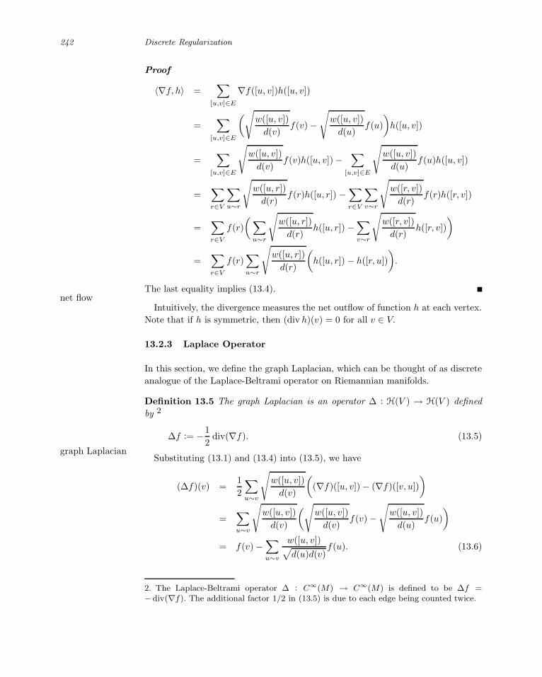
242 Discrete Regularization
Proof
〈∇f, h〉 =∑
[u,v]∈E
∇f([u, v])h([u, v])
=∑
[u,v]∈E
(√w([u, v])
d(v)f(v) −
√w([u, v])
d(u)f(u)
)h([u, v])
=∑
[u,v]∈E
√w([u, v])
d(v)f(v)h([u, v]) −
∑
[u,v]∈E
√w([u, v])
d(u)f(u)h([u, v])
=∑
r∈V
∑
u∼r
√w([u, r])
d(r)f(r)h([u, r]) −
∑
r∈V
∑
v∼r
√w([r, v])
d(r)f(r)h([r, v])
=∑
r∈V
f(r)
(∑
u∼r
√w([u, r])
d(r)h([u, r]) −
∑
v∼r
√w([r, v])
d(r)h([r, v])
)
=∑
r∈V
f(r)∑
u∼r
√w([u, r])
d(r)
(h([u, r]) − h([r, u])
).
The last equality implies (13.4).net flow
Intuitively, the divergence measures the net outflow of function h at each vertex.
Note that if h is symmetric, then (div h)(v) = 0 for all v ∈ V.
13.2.3 Laplace Operator
In this section, we define the graph Laplacian, which can be thought of as discrete
analogue of the Laplace-Beltrami operator on Riemannian manifolds.
Definition 13.5 The graph Laplacian is an operator ∆ : H(V ) → H(V ) defined
by 2
∆f := −1
2div(∇f). (13.5)
graph LaplacianSubstituting (13.1) and (13.4) into (13.5), we have
(∆f)(v) =1
2
∑
u∼v
√w([u, v])
d(v)
((∇f)([u, v]) − (∇f)([v, u])
)
=∑
u∼v
√w([u, v])
d(v)
(√w([u, v])
d(v)f(v) −
√w([u, v])
d(u)f(u)
)
= f(v) −∑
u∼v
w([u, v])√d(u)d(v)
f(u). (13.6)
2. The Laplace-Beltrami operator ∆ : C∞(M) → C∞(M) is defined to be ∆f =−div(∇f). The additional factor 1/2 in (13.5) is due to each edge being counted twice.

13.2 Discrete Analysis 243
self-adjoint
positive definite
The graph Laplacian is a linear operator because both the gradient and divergence
operators are linear. Furthermore, the graph Laplacian is self-adjoint,
〈∆f, g〉 =1
2〈− div(∇f), g〉 =
1
2〈∇f,∇g〉 =
1
2〈f,− div(∇g)〉 = 〈f,∆g〉,
and positive semi-definite:
〈∆f, f〉 =1
2〈− div(∇f), f 〉 =
1
2〈∇f,∇f〉 = S2(f) ≥ 0. (13.7)
It immediately follows from (13.7) that
Theorem 13.6 2∆f = DfS2.
Remark 13.7 Equation (13.6) shows that our graph Laplacian defined by (13.5)
is identical to the Laplace matrix in (Chung, 1997) defined to be ∆ = D−1/2(D −W )D−1/2, where D is a diagonal matrix with D(v, v) = d(v), and W a matrix
with W (u, v) = w([u, v]) if [u, v] is an edge and W (u, v) = 0 otherwise. It is worthLaplace matrix
mentioning that the matrix L = D − W is often referred to as the combinatorial
(or unnormalized) graph Laplacian, or simply the graph Laplacian. Obviously, this
Laplacian can also be derived in a similar way. Specifically, define a graph gradient
by
(∇f)([u, v]) :=√
w([u, v])(f(v) − f(u)), for all [u, v] ∈ E,
and then the rest proceeds as the above.
Remark 13.8 For the connection between graph Laplacians (including the Lapla-
cian we presented here) and the usual Laplacian in continuous case, we refer the
reader to (von Luxburg et al., 2005; Hein et al., 2005; Bousquet et al., 2004). Theconvergence
main point is that, if we assume the vertices of a graph are identically and indepen-
dently sampled from some unknown but fixed distribution, when the sampling size
goes to infinity, the combinatorial graph Laplacian does not converge to the usual
Laplacian unless the distribution is uniform.
13.2.4 Curvature Operator
In this section, we define the graph curvature which can be regarded as a discrete
analogue of the mean curvature in continuous case.
Definition 13.9 The graph curvature is an operator κ : H(V ) → H(V ) defined by
κf := −1
2div
( ∇f
‖∇f‖
). (13.8)
graph curvature

244 Discrete Regularization
Substituting (13.1) and (13.4) into (13.8), we obtain
(κf)(v) =∑
u∼v
√w([u, v])
d(v)
( ∇f
‖∇f‖([u, v]) − ∇f
‖∇f‖([v, u])
)
=∑
u∼v
w([u, v])√d(v)
[1
‖∇uf‖
(f(v)√d(v)
− f(u)√d(u)
)− 1
‖∇vf‖
(f(u)√d(u)
− f(v)√d(v)
)]
=1
2
∑
u∼v
w([u, v])√d(v)
(1
‖∇uf‖ +1
‖∇vf‖
)(f(v)√d(v)
− f(u)√d(u)
). (13.9)
Unlike the graph Laplacian (13.5), the graph curvature is a nonlinear operator.
As in theorem 13.6, we have
Theorem 13.10 κf = DfS1.
Proof
(DfS1)(v) =∑
u∼v
[w([u, v])
‖∇uf‖
(f(v)
d(v)− f(u)√
d(u)d(v)
)+
w([u, v])
‖∇vf‖
(f(v)
d(v)− f(u)√
d(u)d(v)
)]
=∑
u∼v
w([u, v])
(1
‖∇uf‖ +1
‖∇vf‖
)(f(v)
d(v)− f(u)√
d(u)d(v)
)
=∑
u∼v
w([u, v])√d(v)
(1
‖∇uf‖ +1
‖∇vf‖
)(f(v)√d(v)
− f(u)√d(u)
).
Comparing the last equality with (13.9) completes the proof.
13.2.5 p-Laplace Operator
In this section, we generalize the graph Laplacian and curvature to an operator,
which can be thought of as the discrete analogue of the p-Laplacian in continuous
case (Hardt and Lin, 1987; Heinonen et al., 1993).
Definition 13.11 The graph p-Laplacian is an operator ∆p : H(V ) → H(V )
defined by
∆pf := −1
2div(‖∇f‖p−2∇f). (13.10)
graph
p-LaplacianClearly, ∆1 = κ, and ∆2 = ∆. Substituting (13.1) and (13.4) into (13.10), we
obtain
(∆pf)(v) =1
2
∑
u∼v
w([u, v])√d(v)
(‖∇uf‖p−2+‖∇vf‖p−2)
(f(v)√d(v)
− f(u)√d(u)
), (13.11)
which generalizes (13.6) and (13.9).
As before, it can be shown that
Theorem 13.12 p∆pf = DfSp.

13.3 Discrete Regularization 245
Remark 13.13 There is much literature on the p-Laplacian in continuous case.
We refer the reader to (Heinonen et al., 1993) for a comprehensive study. There
is also some work on the discrete analogue of the p-Laplacian, e.g., see (Yamasaki,
1986), where it is defined as
∆pf(v) =1
gp(v)
∑
u∼v
wp−1([u, v])|f(u) − f(v)|p−1 sign(f(u) − f(v)),
where gp(v) =∑
u∼v wp−1([u, v]) and p ∈ [2,∞[. Note that p = 1 is not allowed.
13.3 Discrete Regularization
Given a graph G = (V, E) and a label set Y = 1,−1, the vertices v in a subset
S ⊂ V are labeled as y(v) ∈ Y. Our goal is to label the remaining unlabeled vertices,
i.e., the vertices in the complement of S. Assume a classification function f ∈ H(V ),
which assigns a label sign f(v) to each vertex v ∈ V. Obviously, a good classification
function should vary as slowly as possible between closely related vertices while
changing the initial label assignment as little as possible.discrete
regularization Define a function y ∈ H(V ) with y(v) = 1 or −1 if vertex v is labeled as positive or
negative respectively, and 0 if it is unlabeled. Thus we may consider the optimization
problem
f∗ = argminf∈H(V )
Sp(f) + μ‖f − y‖2, (13.12)
where μ ∈]0,∞[ is a parameter specifying the tradeoff between the two competing
terms. It is not hard to see that the objective function is strictly convex, and hence
by standard arguments in convex analysis the optimization problem has a unique
solution.
13.3.1 Regularization with p = 2
When p = 2, the following equation can derived from theorem 13.6.
Theorem 13.14 The solution of (13.12) satisfies that
∆f∗ + μ(f∗ − y) = 0.
The equation in the theorem can be thought of as discrete analogue of the Euler-
Lagrange equation. It is easy to see that we can obtain a closed-form solution
f∗ = μ(∆ + μI)−1y, where I denotes the identity operator. Define the functionheat diffusion
c : E → R+ by
c([u, v]) =1
1 + μ
w([u, v])√d(u)d(v)
, if u = v; and c([v, v]) =μ
1 + μ. (13.13)

246 Discrete Regularization
We can show that the iteration
f (t+1)(v) =∑
u∼v
c([u, v])f (t)(v) + c([v, v])y(v), for all v ∈ V, (13.14)
where t indicates the iteration step, converges to a closed-form solution (Zhou
et al., 2004). Moreover, the iterative result is independent of the setting of the
initial value. The iteration can be intuitively thought of as a sort of information
diffusion. At every step, each node receives the values from its neighbors, which
are weighted by the normalized pairwise relationships. At the same time, they also
retain some fraction of their values. The relative amount by which these updates
occur is specified by the coefficients defined in (13.13). In what follows, this iteration
approach will be generalized to arbitrary p.
Remark 13.15 It is easy to see that the regularizer of p = 2 can be rewritten into
1
2
∑
u,v
w([u, v])
(f(u)√d(u)
− f(v)√d(v)
)2
, (13.15)
which we earlier suggested for transductive inference (Zhou et al., 2004). A closelyunnormalized
regularizer related one is
1
2
∑
u,v
w([u, v])(f(u) − f(v))2, (13.16)
which appeared in (Joachims, 2003; Belkin et al., 2004a; Zhu et al., 2003b). From
the point of view of spectral clustering, (13.15) can be derived from the normalized
cut (Shi and Malik, 2000), and corresponds to the (normalized) graph Laplacian
(13.5); and (13.16) is derived from the ratio cut (Hagen and Kahng, 1992), and
corresponds to the combinatorial graph Laplacian (see also remark 13.7). On many
real-world experiments, a remarkable difference between these two regularizers is
that the transductive approaches based on (13.16) (Joachims, 2003; Zhu et al.,
2003b) strongly depend on the prior knowledge of proportion among different classes
while the approach based on (13.15) (Zhou et al., 2004) can work well without such
prior knowledge. For more details, we refer the reader to chapter 21 (Analysis of
Benchmarks) and chapter 11 (Label Propagation and Quadratic Criterion).
Remark 13.16 One can construct many other similar regularizers. For instance,locally linear
embedding
regularizer
one might consider (Roweis and Saul, 2000)
1
2
∑
u,v
(f(v) −
∑
u∼v
p([u, v])f(u)
)2
, (13.17)
where the function p : E → R+ is defined to be p([u, v]) = w([u, v])/d(u). Note that
p is not symmetric. This regularizer measures the difference of function f at vertex
v, and the average of f on the neighbors of v.

13.3 Discrete Regularization 247
13.3.2 Regularization with p = 1
When p = 1, it follows from theorem 13.10 that
Theorem 13.17 The solution of (13.12) satisfies that
κf∗ + 2μ(f∗ − y) = 0.
As we have mentioned before, the curvature κ is a nonlinear operator, and we are
not aware of any closed-form solution for this equation. However, we can construct
an iterative algorithm to obtain the solution. Substituting (13.9) into the equation
in the theorem, we have
∑
u∼v
w([u, v])√d(v)
(1
‖∇uf∗‖ +1
‖∇vf∗‖
)(f∗(v)√
d(v)− f∗(u)√
d(u)
)+2μ(f∗(v)− y(v)) = 0.
(13.18)
Define the function m : E → R+ by
m([u, v]) = w([u, v])
(1
‖∇uf∗‖ +1
‖∇vf∗‖
). (13.19)
Then
∑
u∼v
m([u, v])√d(v)
(f∗(v)√
d(v)− f∗(u)√
d(u)
)+ 2μ(f∗(v) − y(v)) = 0,
which can be transformed into(∑
u∼v
m([u, v])
d(v)+ 2μ
)f∗(v) =
∑
u∼v
m([u, v])√d(u)d(v)
f∗(u) + 2μy(v).
Define the function c : E → R+ bycurvature flow
c([u, v]) =
m([u, v])√d(u)d(v)
∑u∼v
m([u, v])
d(v)+ 2μ
, if u = v, (13.20)
and
c([v, v]) =2μ
∑u∼v
m([u, v])
d(v)+ 2μ
. (13.21)
Then
f∗(v) =∑
u∼v
c([u, v])f∗(v) + c([v, v])y(v). (13.22)

248 Discrete Regularization
Thus we can use the iteration
f (t+1)(v) =∑
u∼v
c(t)([u, v])f (t)(v) + c(t)([v, v])y(v), for all v ∈ V (13.23)
to obtain the solution, in which the coefficients c(t) are updated according to (13.20)
and (13.19). It can be shown that this iterative result is independent of the setting of
the initial value. Compared with the iterative algorithm (13.14) in the case of p = 2,
the coefficients in the present method are adaptively updated at each iteration, in
addition to the function being updated.
13.3.3 Regularization with Arbitrary p
For arbitrary p, it follows from theorem 13.12 that
Theorem 13.18 The solution of (13.12) satisfies that
p∆pf∗ + 2μ(f∗ − y) = 0.
We can construct a similar iterative algorithm to obtain the solution. Specifically,general diffusion
f (t+1)(v) =∑
u∼v
c(t)([u, v])f (t)(v) + c(t)([v, v])y(v), for all v ∈ V, (13.24)
where
c(t)([u, v]) =
m(t)([u, v])√d(u)d(v)
∑u∼v
m(t)([u, v])
d(v)+
2μ
p
, if u = v, (13.25)
and
c(t)([v, v]) =
2μ
p
∑u∼v
m(t)([u, v])
d(v)+
2μ
p
, (13.26)
and
m(t)([u, v]) =w([u, v])
p(‖∇uf (t)‖p−2
+ ‖∇vf(t)‖p−2
). (13.27)
It is easy to see that the iterative algorithms in sections 13.3.1 and 13.3.2 are the
special cases of this general one with p = 2 and p = 1 respectively. Moreover, it is
interesting to note that p = 2 is a critical point.

13.4 Conclusion 249
13.4 Conclusion
In this chapter, we proposed the discrete analogues of a family of differential
operators, and the discrete analogue of classical regularization theory based on
those discrete differential operators. A family of transductive inference algorithms
corresponding to different discrete differential operators was naturally derived from
the discrete regularization framework.
There are many possible extensions to this work. One may consider defining dis-
crete high-order differential operators, and then building a regularization framework
that can penalize high-order derivatives. One may also develop a parallel framework
on directed graphs (Zhou et al., 2005b), which model many real-world data struc-
tures, such as the World Wide Web. Finally, it is of interest to explore the properties
of the graph p-Laplacian as the nonlinear extension of the usual graph Laplacian,
since the latter has been intensively studied, and has many nice properties (Chung,
1997).


14 Semi-Supervised Learning with Conditional
Harmonic Mixing
Christopher J. C. Burges [email protected]
John C. Platt [email protected]
Recently graph-based algorithms, in which nodes represent data points and links
encode similarities, have become popular for semi-supervised learning. In this
chapter we introduce a general probabilistic formulation called conditional harmonic
mixing (CHM), in which the links are directed, a conditional probability matrix is
associated with each link, and where the numbers of classes can vary from node
to node. The posterior class probability at each node is updated by minimizing
the Kullback-Leibler (KL) divergence between its distribution and that predicted
by its neighbors. We show that for arbitrary graphs, as long as each unlabeled
point is reachable from at least one training point, a solution always exists, is
unique, and can be found by solving a sparse linear system iteratively. This result
holds even if the graph contains loops, or if the conditional probability matrices
are not consistent. We show how, given a classifier for a task, CHM can learn its
transition probabilities. Using the Reuters database, we show that CHM improves
the accuracy of the best available classifier, for small training set sizes.
14.1 Introduction
Graphical models provide a powerful framework for approaching machine learning
problems. Two common examples are probabilistic graphical models (Jordan, 1999)
and semi-supervised learning on graphs (see chapter 11 and (Zhu and Ghahramani,
2002; Zhu et al., 2003b; Zhou et al., 2004)) and which we refer to here as Laplacian
SSL. Graphs have been used as a general representation of preference relations
in ranking problems (Dekel et al., 2004) and play a role in various approaches to
dimensional reduction (Burges, 2005). In this chapter, we propose a new graph-conditional
harmonic mixing based approach to semi-supervised learning called conditional harmonic mixing
(CHM).

252 Semi-Supervised Learning with Conditional Harmonic Mixing
Probabilistic graphical models such as Bayes nets write a probability distribution as
a product of conditionals, which live on the nodes; the arcs encode conditional in-
dependence assumptions. Laplacian semi-supervised learning (SSL) is more closely
related to random walks on networks (Doyle and Snell, 1984): each arc encodes the
similarity between the nodes at its endpoints, and the goal is to use neighborhood
structure to guide the choice of classification (or regression, clustering, or ranking)
function. For Laplacian SSL models, the probabilistic interpretation is somewhat
indirect (Zhu et al., 2003b); for probabilistic graphical models, it is central. In
CHM we propose an intermediate model, where both a probabilistic interpretation
and Laplacian SSL are central. In CHM, no attempt is made to model an overall
joint density; we are only interested, ultimately, in the class-conditional posteriors.
Although it is assumed that there exists some underlying joint, the model itself
is viewed as an approximation; in particular, the conditional probabilities may be
approximations, and as a result, inconsistent (i.e., no joint may exist for which
they are the conditionals). This results in some striking differences between CHM
and well-known probabilistic graphical models such as Bayes nets: for example, in
CHM, the process of learning the posteriors, given the conditionals, converges to
a global optimum via a straightforward iterative optimization procedure, whatever
the structure of the graph (in particular, even if there are loops), provided only that
there exists a path to each unlabeled point from at least one labeled point. In this
regard, CHM is similar to dependency networks (Heckerman et al., 2001). In CHM,
as in Laplacian SSL, each node corresponds to a random variable, but unlike the
original Laplacian SSL, the arcs are directed , and each arc carries a matrix whichdirected graphs
models a conditional probability.1 The matrices can even be rectangular, which
corresponds to the posteriors at different nodes corresponding to different numbers
of classes for that random variable. We will also investigate learning the condi-
tional probability matrices themselves from data. In this chapter we will consider
CHM models for classification, but the same ideas could be extended for regression,
clustering, ranking, etc.
14.1.1 Conditional Harmonic Mixing: Motivation
CHM is a highly redundant model, in that for a “perfect” CHM model of a given
problem, the posterior for a given node can be computed from the posterior at any
adjacent node, together with the conditional probability matrix on the arc joining
them. However this is an idealization: CHM handles this by asking that the posterior
at a given node be that distribution such that the number of bits needed to describe
the distributions predicted at that node, by the adjacent nodes, is minimized. This
is accomplished by minimizing a Kullback-Leibler (KL) divergence (see below).Kullback-Leibler
divergence Building on an idea proposed in Zhu et al. (2003b), CHM can also be used to
improve the accuracy of another, given base classifier.
1. Recently, Zhou et al. (2005b) have extended Laplacian SSL to the case of directed arcs.

14.1 Introduction 253
In the graphical approaches to semi-supervised learning of Zhu and Ghahramani
(2002); Zhu et al. (2003b), and Zhou et al. (2004) (see also chapter 11), the
underlying intuition is that the function should vary smoothly across the graph,
so that closely clustered points tend to be assigned similar function values (the
“clustering assumption”). This leads to the use of undirected arcs in the graph,
since the graph is used essentially to model the density. However, there is a second
intuition that we wish to add, and that is of the propagation of information.
Consider the graph shown in figure 14.1, left panel (in this chapter, filled (unfilled)
circles represent labeled (unlabeled) points), where both arcs have the same weight.
In the harmonic solutions of Zhu and Ghahramani (2002); Zhu et al. (2003b), and
Zhou et al. (2004), the state of node 2 is the weighted average of its neighbors.
However, in this particular graph, it seems strange to have node 2 care about the
state of node 3, since from the information propagation point of view, all of the
label information propagates out from node 1, and all label information about node
3 has already passed through node 2. By making the arcs directed, as in the right
panel, this problem can be addressed with no loss of generality, since an undirected
arc between nodes A and B can be simulated by adding arcs A→B and B→A.
1 2 3 1 2 3
Figure 14.1 Directional arcs for information flow.
A second reason for using directed arcs is that the relations between points can
themselves be asymmetric (even if both are unlabeled). For example, in k-nearest
neighbor, if point A is the nearest neighbor of point B, point B need not be that of
point A. Such asymmetric relations can be captured with directed arcs.
CHM shares with Laplacian SSL the desirable property that its solutions areharmonic
solutions harmonic, and unique, and can be computed iteratively and efficiently. It shares with
Bayesian graphical models the desirable property that it is a probabilistic model
from the ground up. We end this section with a simple but useful observation, but
first we must introduce some notation. Suppose nodes i and j (i, j ∈ 1, . . . , N) are
connected by a directed arc from i to j (throughout, we will index nodes by i, j, k
and vector indices by a, b). We will represent the posterior at any node k as the
vector P (Xk = Ma) ≡ Pk (so that Pk is a vector indexed by a), and the conditional
on the arc as P (Xj |Xi, G) ≡ Pji (so that Pji is a matrix indexed by the class index
at node j and the class index at node i). Then the computation of i’s prediction of
the posterior at j is just the matrix vector multiply PjiPi.=
∑b(Pji)ab(Pi)b. Note
that all conditional matrices are also conditioned on the training data, the graph
structure, and other factors, which we denote collectively by G. We emphasize that
the number of classes at different nodes can differ, in which case the conditional
matrices joining them will be rectangular. Note also that the Pji are column

254 Semi-Supervised Learning with Conditional Harmonic Mixing
stochastic matrices. Similarly we will call any vector whose components are a
non-negative partition of unity a stochastic vector. Then we have the following
observation.
Proposition 14.1 Given any two stochastic vectors Pi and Pj, there always exists
a conditional probability matrix Pij such that Pi = PijPj.
This follows trivially from the choice (Pij)ab = (Pi)a ∀b, and just corresponds to
the special case that the probability vectors Pi and Pj are independent. This shows
that CHM is able, in principle, to model any set of posteriors on the nodes, and
that some form of regularization will therefore be needed if we expect, for example,
to learn nontrivial matrices Pij given a set of posteriors Pi. We will impose this
regularization by partitioning the Na arcs in the graph into a small number n of
equivalence classes, where n ≪ Na, such that arcs in a given equivalence class are
to have the same Pij . In this chapter, we will use nearest-neighbor relations to
determine the equivalence classes.
14.1.2 Related Work
Zhu and Ghahramani (2002); Zhu et al. (2003b), and Zhou et al. (2004) introduce
Laplacian SSL for transductive learning using graphs (see also chapter 11). Eachtransductive
learning link is given a scalar weight that measures the similarity between the data points
attached to the nodes at that link’s endpoints, and each node has a scalar value. The
objective function is a weighted sum of squared differences in function values be-
tween pairs of nodes, with positive weights; minimizing this encourages the modeled
function to vary slowly across nodes. The solution is a harmonic function (Doyleharmonic
function and Snell, 1984) in which each function value is the weighted sum of neighboring
values. The function is thresholded to make the classification decision. In contrast
to Laplacian SSL, at the solution, for nondiagonal conditional probability matri-
ces, the CHM conditional harmonic property generates extra additive terms in the
function on the nodes, which are not present in the Gaussian field solution (which
is homogeneous in the function values). The two methods coincide only when the
random variables at all nodes correspond to just two classes, when the conditional
probability matrices in CHM are 2 × 2 unit matrices, where all the weights in the
Gaussian random field are unity, and where all nodes are joined by directed arcs
in both directions. Finally, one concrete practical difference is that CHM can han-
dle one-sided classification problems, where training data from only one class are
available, by using conditional posterior matrices other than unit matrices. In this
case, the objective function in (Zhu et al., 2003b) is minimized by attaching the
same label to all the unlabeled data. However, either method can handle one-sided
classification problems by leveraging results from an existing one-sided classifier;
we will explore this method below.
Zhu et al. (2003c) embed the label propagation work in a probabilistic framework
by showing that the model can be viewed in terms of Gaussian processes. However,Gaussian process
to establish the connection, extra assumptions and approximations are required: the

14.2 Conditional Harmonic Mixing 255
inverse covariance matrix must be regularized; an extra set of unobserved random
variables, which give rise to the labels via a sigmoid conditional, are introduced; and
the posteriors must be approximated (the authors use the Laplace approximation).
CHM, by contrast, is inherently a probabilistic model.
Directed graph models for semi-supervised learning were also considered in (Zhou
et al., 2005b). However, in that work, the kinds of graphs considered were specific
to a weblike application, with nodes split into hubs and authorities, and with the
fundamental assumption that the similarity of two nodes in the graph is defined by
their colinkage (either from parents or children). Again, the aim of the model is to
require that the modeled function vary slowly across “similar” nodes, so the notion
of information propagation described above does not play a direct role; the model
is also not a probabilistic one. More recently, semi-supervised learning on directed
graphs was also studied from a more general point of view in (Zhou et al., 2005a).
Finally we emphasize the main differences between CHM and probabilistic graphical
models such as Bayes nets and Markov random fields (MRFs). Belief nets and MRFsBayes nets
use the graph structure to encode conditional independence assumptions about the
random variables in the model, whereas CHM uses the (redundant) graph structure
to model both the flow of information from the training data, and the smoothness
assumptions on the functions being modeled. Evaluating belief nets (for example,
using belief propagation) in the presence of loops in the graph gets complicated
quickly, whereas, as we shall see, CHM converges under general conditions, even
in the presence of loops. However, both approaches share the fact that they are
probabilistic models.
14.2 Conditional Harmonic Mixing
The structure of the CHM graph will depend on the problem at hand; however,
all graphs share the weak constraint that for every2 test node i, there must exist
a path in the graph joining i with a training node. We will refer to such nodes as
label-connected, and to the graph as a whole as label-connected if every test node
in the graph is label-connected. A neighbor of a given node i is defined to be any
node which is adjacent to node i, where “adjacent” means that there exists an arc
from j to i.
We use the following notation: we assume that the random variable at node i has
Mi states (or classes), and that the arc from node i to node j carries an Mj × Mi
conditional probability matrix Pji. We adopt the convention that Pji is the Mj×Mi
matrix of all zeros if there is no arc from node i to node j. We denote the posterior
at node i by the vector Pi ∈ RMi for unlabeled nodes, and by Qi ∈ R
Mi for labeled
2. For readability we use the indices i, j to denote the nodes themselves, since thesequantities appear frequently as subscripts. We use the terms “test node” and “unlabelednode” interchangeably.

256 Semi-Supervised Learning with Conditional Harmonic Mixing
nodes. Denote the set of labeled nodes by L, with l.= |L|, and the set of unlabeled
nodes by U, with u.= |U|, let M(i) (N(i)) denote the set of indices of labeled
(unlabeled) nodes adjacent to node i, and define I = M ∪ N with n(i).= ‖I(i)‖.
Finally, for node i, let p(i) be the number of incoming arcs from adjacent test nodes,
and let q(i) be the number of incoming arcs from adjacent train nodes.
14.2.1 The CHM Update Rule
A given node in the graph receives an estimate of its posterior from each of
its neighbors. These estimates may not agree. Suppose that the hypothesized
distribution at node i is Qi, and let the estimates from its n(i) neighbors be Pj , j ∈I(i), so that Pj = PjkPk for each k ∈ I(i). Given Qi, the number of bits required toKullback-Leibler
divergence describe the distributions Pj is∑
jH(Pj)+D(Pj |Qi), where H is the entropy and
D the KL divergence. Since we wish to use Qi to describe the combined distributions
Pj as closely as possible, we require that this number of bits be minimized. For fixed
Pj , this is accomplished by setting (Qi)a = (1/n(i))∑n(i)
j=1(Pj)a. A function on a
graph is called harmonic (Doyle and Snell, 1984; Zhu et al., 2003b) if at each internalharmonic
function node the value of the function is the (possibly weighted) mean of the values at its
neighboring points (an internal node, as opposed to a boundary node, is one whose
function value is not fixed; below we will just use the terms “unlabeled node” and
“labeled node” for internal and boundary nodes). Assuming that a solution exists,
then at the solution, the posterior at a given node is the weighted mean of the
posteriors of its neighbors, where the weights are conditional probability matrices;
hence the name “conditional harmonic mixing.”
14.3 Learning in CHM Models
14.3.1 A Simple Model
It is useful to examine a simple model to fix ideas and to demonstrate a simple
convergence proof. Consider the three-point graph shown in figure 14.2, with one
labeled and two unlabeled nodes, and where to simplify the exposition we take the
number of classes at each node to be C.
The consistency conditions arising from the above update rule are
(−1 1
2P1212P13
12P21 −1 1
2P23
)⎛⎜⎜⎝
P1
P2
P3
⎞⎟⎟⎠ = 0, (14.1)
where P3 = (1, 0, 0, . . . ) and where the ones in the matrices represent unit matrices.
We wish to prove four properties of these equations, for any choice of conditional
probability matrices P23, P21, P12, and P13: first, that a solution always exists;
second, that it is unique; third, that it results in stochastic vectors for the solution

14.3 Learning in CHM Models 257
1
2
P12
P13
P23
P21 3
Figure 14.2 A simple three-point CHM graph.
P2 and P3; and fourth, that Jacobi iterates will converge to it (by solving with Jacobi
iterates, we will be able to take advantage of the sparseness of larger problems, as
we will see below). Rearranging, we have
(1 − 1
2P12
− 12P21 1
)(P1
P2
)=
1
2
(P13P3
P23P3
). (14.2)
The equations will always take this general form, where the matrix on the left is
square (but not necessarily symmetric) and of side Cu, and where the left-hand
side depends only on the unlabeled points (whose posteriors we wish to find) and
the right, only on the labeled points. Define
b.=
1
2
(P13P3
P23P3
), M
.=
(1 0
0 1
), N
.=
(0 1
2P12
12P21 0
)(14.3)
and consider the following iterative algorithm for finding the solution, where x(0)
is arbitrary:
Mx(k+1) = Nx(k) + b. (14.4)
With the above definitions, this is a Jacobi iteration (Golub and Van Loan, 1996,
p. 510), and we have:
Theorem 14.2 (Golub and Van Loan (1996, Theorem 10.1.1)) Suppose
b ∈ Rd and ∆
.= M − N ∈ R
d×d is nonsingular. If M is nonsingular and the
spectral radius of M−1N satisfies the inequality ρ(M−1N) < 1, then the iterates
x(k) defined by (14.4) converge to x = ∆−1b for any starting vector x.
Since N here is one-half times a column-stochastic matrix, its eigenvalues havestochastic vectors
and matrices absolute value at most 12 , so ρ(M−1N) < 1. Hence for this graph, a solution
always exists and is unique. If we start with stochastic vectors everywhere (chosen
arbitrarily on the unlabeled nodes), then they will remain stochastic since each
Jacobi iterate maintains this property, and the solution will be stochastic.3 Note
3. In fact this is true even if the initial vectors on the unlabeled nodes are chosen

258 Semi-Supervised Learning with Conditional Harmonic Mixing
also that the matrix M−N is diagonally dominant, and so has an inverse. However,
for the general case, N may not be proportional to a column stochastic matrix, and
furthermore M − N may not be diagonally dominant; we will need a more general
argument.
14.3.2 A General Convergence Proof
At the CHM solution, for each node i, we have the consistency conditions
Pi −1
p(i) + q(i)
⎛
⎝∑
j∈N(i)
PijPj
⎞
⎠ =1
p(i) + q(i)
⎛
⎝∑
j∈M(i)
PijQj
⎞
⎠ , (14.5)
where the right-hand side is defined to be zero if M(i) = ∅. Let p =∑
i∈U Mi, and
define a block matrix A ∈ Rp×p with ones along the diagonal and whose off-diagonal
elements, which are either zero matrices or are the matrices 1p(i)+q(i)Pij , are chosen
so that (14.5) can be written as
AP = Q, (14.6)
where P, Q ∈ Rp. Note that the right-hand side of (14.6) is determined by the
training data, that all conditional probability matrices associated with unlabeled-
unlabeled arcs are in A, and that all conditional probability matrices associated
with labeled-unlabeled arcs are in Q. Thus (14.5) corresponds to the ith row of
(14.6) and encapsulates Mi equations. Define the kth Jacobi iterate byJacobi iterations
P(k)i =
1
p(i) + q(i)
⎛
⎝∑
j∈N(i)
PijP(k−1)j
⎞
⎠ +1
p(i) + q(i)
⎛
⎝∑
j∈M(i)
PijQj
⎞
⎠ . (14.7)
Referring to theorem 14.2, we see that in this case, A.= M − N where M = I and
Nij.= 1
p(i)+q(i)Pij (recall that we define Pij to be the matrix of all zeros, if there is
no arc from node j to node i), and b is the second term on the right-hand side of
(14.7). Then the kth Jacobi iterate takes the form MP (k) = NP (k−1) + b. We can
now state:
Theorem 14.3 Consider a label-connected CHM graph with l labeled nodes. As-
sume that the vectors at the labeled nodes are fixed and stochastic. Then a solution
to the corresponding CHM equations, (14.6), always exists and is unique. Further-
more, at the solution, the vector P ∗i ∈ R
Mi at the ith unlabeled node is stochastic for
all i, and the Jacobi iterates on the graph will always converge to the same solution,
regardless of the initial values given to the Pi.
We present the proof in the proof-style advocated by Lamport (1993).
arbitrarily, by theorem 14.2, since the solution is unique.

14.3 Learning in CHM Models 259
Proof
1. Assume: the CHM graph is label-connected.
2. ρ(N) < 1.
2.1. Proof Consider the eigenvalue equation:
Nµ = λµ. (14.8)
Just as we view N as a block matrix whose ith, jth element is the matrix1
p(i)+q(i)Pij , similarly view µ as a vector whose ith element is a vector of
dimension Mi. Then let µi be that component of µ whose L1 norm is largest (or
any such component if there are more than one) and consider the corresponding
rows of (14.8), which encapsulates the Mi equations
1
p(i) + q(i)
⎛
⎝∑
j∈N(i)
Pijµj
⎞
⎠ = λµi. (14.9)
2.1.1 Assume: q(i) > 0 and i : ‖µi‖1 ≥ ‖µj‖1 ∀j.
2.1.1.1 Since Pij is column stochastic, it has unit L1 norm. Thus∥∥∥∥∥∥
∑
j∈N(i)
Pijµj
∥∥∥∥∥∥1
≤∑
j∈N(i)
∥∥Pijµj
∥∥1
≤∑
j∈N(i)
‖Pij‖1
∥∥µj
∥∥1
=∑
j∈N(i)
‖µj‖1
≤ p(i)‖µi‖1.
where ‖ · ‖1 denotes the L1 norm, and where the second line follows
from an inequality satisfied by all p norms (Golub and Van Loan,
1996). Since by assumption q(i) ≥ 1, taking the L1 norm of both
sides of (14.9) gives |λ| < 1.
2.1.2 Assume: q(i) = 0 and i : ‖µi‖1 ≥ ‖µj‖1 ∀j.
2.1.2.1 The argument of 2.1.1.1, but with q(i) = 0, gives |λ| ≤ 1, and
if |λ| = 1, then each µj appearing in the sum must have L1 norm

260 Semi-Supervised Learning with Conditional Harmonic Mixing
equal to ‖µi‖1, since for |λ| = 1,
‖µi‖1 =1
p(i)
∥∥∥∥∥∥
∑
j∈N(i)
Pijµj
∥∥∥∥∥∥1
≤ 1
p(i)
∑
j∈N(i)
‖Pijµj‖1
≤ 1
p(i)
∑
j∈N(i)
‖µj‖1 ≤ ‖µi‖1
where the last step follows from the assumption that µi has largest
L1 norm. Thus for each j ∈ N(i), we can repeat the above argument
with µj on the right-hand side of (14.9), and the argument can then
be recursively repeated for each k ∈ N(j), until (14.9) has been
constructed for every node for which a path exists to node i. However
since the graph is label-connected, that set of nodes will include a
test node which is adjacent to a train node. The previous argument,
which assumed that q > 0, then shows that |λ| < 1. Thus, in general
for any label-connected CHM graph, |λ| < 1, and so ρ(N) < 1.
3. A is nonsingular.
3.1 Proof Since ρ(N) < 1, the eigenvalues of N all lie strictly within the unit
circle centered on the origin in the complex plane C. Since N = 1 − A (cf.
(14.6)), if e is an eigenvector of A with eigenvalue λ, then it is an eigenvector
of N with eigenvalue 1−λ, and so since 1−λ lies strictly within the unit circle
centered on the origin in C, λ itself lies strictly within the unit circle centered
on the point 1, 0 ∈ C, so λ = 0. Hence none of A’s eigenvalues vanish, and A
is nonsingular.
4. A solution to the CHM equations exists and is unique.
4.1 Proof Since A is nonsingular, AP = Q has unique solution P = A−1Q.
5. At the solution, the random vector Pi ∈ RMi at each unlabeled node is stochastic,
regardless of its initial value.
5.1 Proof For all unlabeled nodes, choose P(0)i to be that stochastic vector
whose first component is 1 and whose remaining components vanish. Then from
(14.7), by construction P(k)i is stochastic for all k. Hence from theorem 14.2 and
steps 2 and 3 above, the Jacobi iterates will converge to a unique solution, and
at that solution the Pi will be stochastic for all i ∈ N. Finally, by theorem 14.2,
the same (unique) solution will be found regardless of the initial values of the
Pi.
We emphasize the following points:
1. The theorem makes no assumptions on the conditional probability matrices,conditional
probability
matrices

14.4 Incorporating Prior Knowledge 261
beyond the requirement that they be column stochastic. In particular, it does not
assume that the conditional probability matrices on the graph are consistent, that is,
that there exists a joint probability from which all conditionals (or even any subset
of them) could be derived by performing appropriate marginalizations. The CHM
algorithm can therefore be applied using measured estimates of the conditional
probability matrices, for which no precise joint exists.
2. In general A is not symmetric (and need not be row- or column-diagonally
dominant).
3. No structure is imposed on the graph beyond its being label-connected. In
particular, the graph can contain loops.
4. The numbers of classes at each node can differ, in which case the conditional
probability matrices will be rectangular.
5. The model handles probabilistic class labels, that is, the Qi can be arbitrary
stochastic vectors.
6. To improve convergence, Gauss-Seidel iterations should be used, instead ofGauss-Seidel
iterations Jacobi iterations. For Gauss-Seidel iterations, the error tends to zero like ρ(M−1N)k
(Golub and Van Loan, 1996, p. 514).
14.4 Incorporating Prior Knowledge
Suppose that we are given the outputs of a given classifier on the data set. The
classifier was trained on the available labeled examples, but the amount of training
data is limited and we wish to use SSL to improve the results. We can adopt an
idea proposed in (Zhu et al., 2003b), and for each node in the graph, attach an
additional, labeled node, whose label is the posterior predicted for that data point.
In fact CHM allows us to combine several classifiers in this way. This mechanism has
the additional advantage of regularizing the CHM smoothing: the model can apply
more, or less, weight to the original classifier outputs, by adjusting the conditionals
on the arcs. Furthermore, for graphs that fall into several components, some of
which are not label-connected, this method results in sensible predictions for the
disconnected subgraphs; the CHM relaxation can be performed even for subgraphs
containing no labeled data, since the base classifier still makes predictions for those
nodes. In the context of CHM, for brevity we call this procedure of leveraging a baselifting
classifier over a graph “lifting”. We will explore this approach empirically below.
14.5 Learning the Conditionals
We are still faced with the problem of finding the conditional matrices Pij . Here we
propose one method for solving this, which we explore empirically below. Consider
again the simple CHM model shown in figure 14.2, and to simplify the exposition,

262 Semi-Supervised Learning with Conditional Harmonic Mixing
assume that the number of classes at each node is two, and in addition require
that Pl.= P13 = P23 and that Pu
.= P12 = P21 (l, u denoting labeled, unlabeled
respectively). We can parameterize the matrices as
Pl =
(1-v1 v2
v1 1-v2
), Pu =
(1-v3 v4
v3 1-v4
), (14.10)
where 0 ≤ vi ≤ 1 ∀i. Now suppose that the posteriors on every node in figure 14.2
are given, and denote components by, e.g., [P1a, P1b]. In that case, (14.1) may be
rewritten as⎡⎢⎢⎢⎢⎣
−P3a P3b −P2a P2b
P3a −P3b P2a −P2b
−P3a P3b −P1a P1b
P3a −P3b P1a −P1b
⎤⎥⎥⎥⎥⎦
⎡⎢⎢⎢⎢⎣
v1
v2
v3
v4
⎤⎥⎥⎥⎥⎦
=
⎡⎢⎢⎢⎢⎣
2P1a − P2a − P3a
2P1b − P2b − P3b
2P2a − P1a − P3a
2P2b − P1b − P3b
⎤⎥⎥⎥⎥⎦
, (14.11)
which we summarize as Av = z. The matrix A in general need not be square, and
if it is, it may be singular (as it is in this example), and even if it is nonsingular,
computing v by inverting A is not guaranteed to give components vi that lie in the
interval [0, 1]. Thus instead we solve the quadratic programming problem:
arg minv
‖Av − z‖2 subject to 0 ≤ vi ≤ 1 ∀i. (14.12)
The posteriors Pi can simply be the outputs of a given classifier on the problem, if
the classifier outputs are well-calibrated probabilities, or thresholded vectors (whose
elements are 0 or 1) for arbitrary classifiers. To summarize: given some estimate of
the posteriors on every node, the conditional probability matrices on the arcs can
be learned by solving a quadratic programming problem.
14.6 Model Averaging
If sufficient labeled data are available, then a validation set can be used to determine
the optimal graph architecture (i.e., to which neighbors each point should connect).
However, often labeled data are scarce, and in fact semi-supervised learning is really
aimed at this case - that is, when labeled data are very scarce, but unlabeled data
are plentiful. Thus in general for SSL methods it is highly desirable to find a way
around having to use validation sets to choose either the model or its parameters.
In this chapter we will use model averaging: that is, for a given graph, given a
classifier, use CHM to lift its results; then do this for a variety of graphs, and simply
average the posteriors assigned by CHM to each node, across all graphs. This, in
combination with learning the conditionals, makes CHM a largely parameter-free
approach (once a general algorithm for constructing the graphs has been chosen),
although training using many graphs may be more computationally expensive than
using a validation set to choose one.

14.7 Experiments 263
14.7 Experiments
We applied CHM to the problem of text categorization, and to five of the benchmark
classification tasks provided with this book.
14.7.1 Reuters-I Data Set
We applied CHM to the problem of the categorization of news articles in the
Reuters-I data set (Lewis, 1997), with the ModApte split of 9603 training files
and 3744 testing files. Each news article is assigned zero or more labels. Each label
is considered to be an independent classification. We train and test on the ten most
common labels in the data set, which generates ten separate binary classification
problems.
We ran two kinds of classification experiments: one-sided (where only positive
labeled examples are given), and two-sided (where labeled examples of both classesone-sided,
two-sided
classification
are given). The one-sided task is interesting because for some applications, it is much
easier to obtain labeled data of one class than of the other, and few algorithms can
handle training data that contain no examples of one of the classes. For the one-
sided problem we investigated using CHM to lift the Rocchio (inductive) classifier
outputs, since of the methods we considered, only the Rocchio algorithm (Rocchio,Rocchio
algorithm 1971) was appropriate for the one-sided task.
For the two-sided problem, we tested two inductive algorithms and one transduc-
tive algorithm. The two inductive algorithms were a linear support vector machine
(SMV) (Dumais et al., 1998; Drucker et al., 1999) and a mixture of multinomial
conditional models (Nigam et al., 2000). For the mixture model, one multinomialmultinomial
models model is used to model positive examples, while one or more multinomial models are
used to model negative examples. Expectation-maximization (EM) is used to fit the
mixture model to the negative examples. Hyperparameters (C for the linear SVM
and the number of negative multinomials) are set by optimizing the microaveraged
F1 score for the labels for Reuters classes 11–15 on the train/test split. These hy-
perparameters are then used for all ten classes. We also tested the method of Nigam
et al. for transduction using the multinomial mixture model (Nigam et al., 2000).
In that transductive method, EM is used, not only to learn the negative mixture
but also to infer the labels of the unlabeled data. Nigam et al. (2000) introduce
another hyperparameter, which is the fractional weight to assign to each unlabeled
case. This weight is also tuned by optimizing the microaveraged F1 score for classes
11–15.
For all experiments, we assume that the prior for the task is known. For the
lifting arcs (i.e. those arcs joining the extra nodes carrying the classifier posteriors
with the unlabeled nodes), we used unit conditional probability matrices, and we
mapped the base classifier outputs to 0, 1, both for the computation of the learned
matrices, and for the CHM computation itself. We did this because the outputs of
the base classifiers were far from well-calibrated probabilities (or from quantities

264 Semi-Supervised Learning with Conditional Harmonic Mixing
that could be mapped to well-calibrated probabilities) as to be expected for very
small training sets.
For the two-sided case, of the three algorithms used, the SVMs were found to
give the highest overall accuracy, and so we investigated lifting the SVM outputs
with CHM. All of these algorithms make a hard decision about whether a test point
is in, or out of, a class. For all algorithms, we choose the threshold for this decision
point to reproduce the true number of positives on the entire test set (the “known
prior” assumption).
Note that the validation set was not used to tune the CHM model; it was used
only to tune the baseline two-sided classifiers. The motivation for this is that we
wish to see if CHM can be used to improve the accuracy of a given (black box)
classifier, using only very limited training data.
Preprocessing, Graph Construction, and Training Data Each document
is preprocessed into a bag of words: that is, only the frequencies with which words
appear in a document are used as features; the position of a word in a document
is ignored. All words within the text, title, and body of the document are used,
except words within the author or dateline, which are excluded. Words within an
11-word stopword list are also excluded. Every word is stemmed using the Porter
stemmer (Porter, 1980), and the number of occurrences for each stem is computedbag-of-words,
TF, TF-IDF for each document (“term frequency,” or TF). The vector of TF values is then fed
to the multinomial classifiers (which can only accept TF vectors). For all other
classifiers and for constructing the CHM graph, we used TF-IDF features. Here,
IDF (inverse document frequency) (Sparck-Jones, 1972) is the log of the ratio of the
total number of documents to the number of documents in which a stemmed word
appears. This log is multiplied by the term frequency to yield a TF-IDF feature.
The TF-IDF vector for a document is then normalized to lie on the unit sphere.
For CHM, each graph is constructed using a simple nearest-neighbor algorithm:
an arc is added from node i to node j if node i is the kth nearest neighbor of node
j, for all k ≤ K, where K ∈ 1, 3, 5, 7, 9, 11, 15, 20, 25, 30, 40, 50, provided node jnearest neighbor
is not itself a labeled node. The conditional probability matrices for all arcs for a
given k are shared; this imposes a form of regularization on the parameters, and
embodies the idea that k alone should determine the type of link joining the two
nodes. Note that this results in a directed graph which in general has no undirected
equivalent (that is, a pair of unlabeled nodes can have an arc going one way but
not the other, and labeled nodes only have outgoing arcs). The CHM posteriors
at each unlabeled node were then averaged over all twelve graphs to arrive at the
prediction. We tested two CHM algorithms: first, using unit conditional probability
matrices, and second, using learned matrices.
For the one-sided task, we used labeled sets of size 1, 2, 5, 10, 20, 50, and 100,
for each category. For the two-sided task, we used ten times as much labeled data
for each experiment (i.e. labeled sets of size 10, 20, 50, 100, 200, 500 and 1000)
to further explore dependence on training set size. The two-sided training sets are
shared among all classes: we ensure that at least one positive example for each of

14.7 Experiments 265
the ten classes is present in all seven of the training sets.
Results The results are collected below. For the one-sided task, we plot F1 versus
training set size, for Rocchio, Rocchio plus CHM with unit matrices, and Rocchio
plus CHM for learned matrices in figure 14.3. It is interesting that, although on
this task using unit conditional probability matrices gives better mean results, the
learned matrices have lower variance: the results for learned matrices rarely drop
below the Rocchio baseline. Results for the two-sided task are collected in tables 14.1
through 14.7, where we show results for all classifiers and for all categories, as well
as the microaveraged results.
Table 14.1 F1 for top ten categories + microaverage F1, for training set size = 10
Category Multinomial Nigam SVM SVM/CHM SVM/CHM
Mixture Unit Learned
1 0.411 0.411 0.446 0.472 0.457
2 0.477 0.477 0.520 0.603 0.592
3 0.308 0.308 0.463 0.520 0.509
4 0.428 0.428 0.507 0.628 0.538
5 0.246 0.246 0.466 0.515 0.482
6 0.249 0.249 0.151 0.111 0.128
7 0.099 0.099 0.474 0.478 0.507
8 0.223 0.223 0.454 0.504 0.472
9 0.347 0.347 0.242 0.274 0.253
10 0.110 0.110 0.233 0.271 0.233
Microaverage 0.374 0.374 0.446 0.491 0.475
The tables give F1 on the unlabeled subsets only. To determine statistical
significance, we treat F1 score as proportions (similar to (Yang and Liu, 1999)).
To be conservative with our confidence intervals, we treat the number of samples
in the significance test to be the denominator of the F1 score: the number of false
positives plus half the number of errors. Thus, we apply a one-way unbalanced
analysis of variance (ANOVA) to predict correctness of the sample, given a factor
which is the algorithm used. For those experiments where a main effect is found by
ANOVA to be greater than 99% significant, a post hoc test comparing all pairs of
algorithms is performed (using the Tukey-Kramer correction for repeated tests). In
the tables, we boldface the results that are found by the post hoc test to be better
than all of the nonboldface algorithms (at a 99% confidence threshold).
For almost all experiments, the SVM gave higher F1 than the multinomial
mixture or the algorithm of Nigam et al. CHM gives better results than all other
methods, at a 99% confidence threshold, for the case of ten labeled points, and
microaveraged over all data sets.

266 Semi-Supervised Learning with Conditional Harmonic Mixing
1 2 5 10 20 50 100
0.4
0.5
0.6
0.7
0.8
0.9
1
1 2 5 10 20 50 1000.2
0.25
0.3
0.35
0.4
0.45
0.5
0.55
1 2 5 10 20 50 1000.35
0.4
0.45
0.5
0.55
0.6
0.65
0.7
1 2 5 10 20 50 1000.5
0.55
0.6
0.65
0.7
0.75
0.8
0.85
1 2 5 10 20 50 1000.5
0.55
0.6
0.65
0.7
0.75
0.8
0.85
1 2 5 10 20 50 1000.4
0.45
0.5
0.55
0.6
0.65
0.7
0.75
1 2 5 10 20 50 1000.2
0.3
0.4
0.5
0.6
0.7
1 2 5 10 20 50 1000.5
0.55
0.6
0.65
0.7
0.75
0.8
0.85
1 2 5 10 20 50 1000.2
0.3
0.4
0.5
0.6
0.7
0.8
0.9
1 2 5 10 20 50 1000.4
0.45
0.5
0.55
0.6
0.65
0.7
0.75
1 2 5 10 20 50 1000.4
0.45
0.5
0.55
0.6
0.65
0.7
0.75
Figure 14.3 Results for the Rocchio classifiers (solid), Rocchio lifted with CHM,unit conditional matrices (dashed), and Rocchio lifted with learned conditional matrices(dotted). The y-axis is F1, the x-axis, training set size. Graphs are arranged left to rightin order of increasing category. Most graphs have the y-axis range chosen to be 0.35for comparison. The last graph (bottom right) is the microaveraged results over all tencategories.

14.7 Experiments 267
Table 14.2 F1 for top ten categories + microaverage F1, for training set size = 20
Category Multinomial Nigam SVM SVM/CHM SVM/CHM
Mixture Unit Learned
1 0.851 0.869 0.903 0.899 0.908
2 0.663 0.797 0.704 0.723 0.735
3 0.302 0.401 0.453 0.516 0.497
4 0.555 0.571 0.572 0.653 0.609
5 0.385 0.170 0.477 0.563 0.527
6 0.285 0.153 0.148 0.103 0.126
7 0.138 0.132 0.488 0.484 0.507
8 0.227 0.344 0.507 0.521 0.525
9 0.407 0.063 0.228 0.270 0.249
10 0.148 0.284 0.275 0.305 0.280
Microaverage 0.614 0.639 0.678 0.694 0.696
Table 14.3 F1 for top ten categories + microaverage F1, for training set size = 50
Category Multinomial Nigam SVM SVM/CHM SVM/CHM
Mixture Unit Learned
1 0.906 0.917 0.935 0.914 0.923
2 0.655 0.711 0.735 0.741 0.749
3 0.438 0.410 0.579 0.681 0.633
4 0.493 0.512 0.585 0.661 0.626
5 0.268 0.405 0.666 0.697 0.708
6 0.341 0.374 0.514 0.545 0.535
7 0.436 0.404 0.356 0.423 0.379
8 0.394 0.298 0.468 0.532 0.493
9 0.133 0.274 0.256 0.288 0.270
10 0.350 0.312 0.444 0.444 0.444
Microaverage 0.652 0.677 0.734 0.748 0.744

268 Semi-Supervised Learning with Conditional Harmonic Mixing
Table 14.4 F1 for top ten categories + microaverage F1, for training set size = 100
Category Multinomial Nigam SVM SVM/CHM SVM/CHM
Mixture Unit Learned
1 0.917 0.840 0.939 0.912 0.921
2 0.770 0.863 0.798 0.777 0.791
3 0.397 0.596 0.535 0.599 0.559
4 0.637 0.576 0.668 0.674 0.681
5 0.494 0.606 0.728 0.772 0.773
6 0.350 0.333 0.522 0.573 0.542
7 0.485 0.471 0.571 0.579 0.573
8 0.466 0.384 0.680 0.658 0.673
9 0.313 0.335 0.489 0.641 0.595
10 0.333 0.231 0.410 0.410 0.410
Microaverage 0.712 0.715 0.778 0.776 0.778
Table 14.5 F1 for top ten categories + microaverage F1, for training set size = 200
Category Multinomial Nigam SVM SVM/CHM SVM/CHM
Mixture Unit Learned
1 0.921 0.925 0.950 0.916 0.923
2 0.799 0.777 0.829 0.817 0.826
3 0.576 0.542 0.587 0.591 0.583
4 0.586 0.628 0.729 0.737 0.734
5 0.618 0.533 0.754 0.782 0.788
6 0.496 0.463 0.696 0.723 0.715
7 0.574 0.493 0.642 0.552 0.595
8 0.361 0.429 0.721 0.721 0.729
9 0.406 0.371 0.519 0.693 0.580
10 0.275 0.352 0.421 0.421 0.421
Microaverage 0.747 0.736 0.813 0.801 0.804

14.7 Experiments 269
Table 14.6 F1 for top ten categories + microaverage F1, for training set size = 500
Category Multinomial Nigam SVM SVM/CHM SVM/CHM
Mixture Unit Learned
1 0.935 0.935 0.957 0.920 0.930
2 0.781 0.781 0.869 0.835 0.847
3 0.594 0.594 0.691 0.687 0.683
4 0.714 0.714 0.816 0.814 0.820
5 0.696 0.696 0.806 0.821 0.824
6 0.486 0.486 0.704 0.723 0.716
7 0.600 0.600 0.681 0.657 0.679
8 0.565 0.565 0.827 0.775 0.801
9 0.693 0.693 0.704 0.715 0.726
10 0.439 0.439 0.618 0.583 0.610
Microaverage 0.781 0.781 0.856 0.831 0.840
Table 14.7 F1 for top ten categories + microaverage F1, for training set size = 1000
Category Multinomial Nigam SVM SVM/CHM SVM/CHM
Mixture Unit Learned
1 0.938 0.940 0.949 0.926 0.933
2 0.843 0.854 0.888 0.854 0.863
3 0.666 0.626 0.702 0.701 0.693
4 0.691 0.638 0.859 0.827 0.833
5 0.803 0.793 0.828 0.807 0.818
6 0.569 0.565 0.724 0.716 0.720
7 0.682 0.611 0.691 0.679 0.693
8 0.627 0.540 0.841 0.762 0.802
9 0.721 0.760 0.806 0.775 0.783
10 0.398 0.385 0.738 0.719 0.724
Microaverage 0.816 0.807 0.869 0.844 0.852

270 Semi-Supervised Learning with Conditional Harmonic Mixing
14.7.2 Benchmark Data Sets
We also applied CHM to five of the benchmark classification data sets provided with
this book, namely data sets 1, 2, 4, 5, and 7. Each data set contains 1500 points,
with either 10 or 100 labeled points, and comes with a 12-fold validation split: all
results quoted here are microaveraged over the twelve splits. An SVM was used as
the base classifier in these experiments. Given the limited amount of training data,
we chose to use a linear SVM with a very high C parameter (C=1000), which was
effectively a hard-margin classifier.
Preprocessing, Graph Construction, and Training Data For each fold
of each data set, we trained a linear SVM with several different preprocessing
alternatives:
Raw data — no preprocessing
Scaling — after subtracting off the mean, scaling each feature so that they all
have unit variance
Norming — after subtracting off the mean for each feature, scaling each data
point so that they all have unit L2 norm
Sphering — applying PCA to the raw data, and using the latent coordinates as
input
Chopping — as in sphering, but only choosing the top d latent dimensions, where
d is chosen to cover 90% of the variance of the data
One of these alternatives was chosen for each fold, by minimizing a generalization
bound of the resulting SVM. For each fold, we compute
arg mini
R2i ||w2
i ||, (14.13)
where wi is the primal weight vector from the SVM on preprocessing alternative
i, and Ri is the radius of the smallest ball that contains the data (after the ith
preprocessing alternative). We approximate this radius by finding the distance of
the data point that is farther from the mean over the whole data set. This choosing
process usually picks one preprocessing method for all folds of a data set, often
choosing “norming.” However, some data sets (such as data set 4), alternate between
“norming” and “sphering.”
We investigated a different graph construction mechanism from that used for the
Reuters data. We call the algorithm “flood fill”. The flood fill method was found to
give similar results to the basic nearest-neighbor method, but resulted in smaller
graphs, leading to faster experiments (a typical run, for a given data set, for both
training set sizes, and for all 12 splits of the validation set, took approximately
50 minutes on a 3GHz machine). The Flood Fill method works as follows: choose
some fixed positive integer n. Add n directed arcs from each labeled node to its
nearest n unlabeled neighbors; all such arcs are assigned flavor = 1. Call the set

14.7 Experiments 271
of nodes reached in this way N1 (where N1 does not include the training nodes).
For each node in N1, do the same, allowing arcs to land on unlabeled nodes in
N1; assign all arcs generated in this way flavor = 2. At the ith iteration, arcs are
allowed to fall on unlabeled nodes in Ni, but not on nodes Nj , j < i. The process
repeats until either all nodes are reached, or until no further arcs can be added
(note that graphs with disconnected pieces are allowed here). Here we smoothed
(using model averaging) using values for n of 5, 9, 15, 25, and 50. The flood fill
algorithm can create disconnected subgraphs, and since it is not clear how best to
combine outputs of graphs with different connectedness, we simply thresholded the
value at each node after each smoothing step, before taking the average.
Results We present the results in tables 14.8 through 14.11. We chose two
normalizations: the “normed/sphered/chopped” normalization, using the above
bound; or just using the “normed” normalization everywhere, combined with a soft-
margin linear SVM classifier (C=10). As in the Reuters experiments, the prior for
each data set is assumed known. The tables give accuracies on the unlabeled subsets
only. We applied a two-way ANOVA to assess the statistical significance of these
results, where the two factors are the fold number and the algorithm number, and
the prediction of the ANOVA is the correctness of a sample. For those experiments
where a main effect is found by ANOVA to be greater than a 99% significance level,
a post hoc test comparing all pairs of algorithms is performed (using the Tukey-
Kramer correction for repeated tests). Using a 99% (p < 0.01) significance level
for the post hoc comparisons, we find the results shown in the tables, where again
statistical significance is indicated with bold versus normal typeface; the results can
be summarized as follows:
In no case is there a statistically significant difference between the learned
conditional matrices, and the unit matrices, for CHM.
CHM beats the SVM for all conditions for data sets 1 and 2.
For the case of data set 4, with normed-only preprocessing, and l = 100, SVM
beats CHM.
There is no statistically significant difference between results for data set 5.
For data set 7, SVM beats CHM for l = 10, and CHM beats SVM for l = 100.
Discussion This work demonstrates that CHM can be used to improve the
performance of the best available classifier, on several data sets, when labeled
data are limited. However, the improvement is not uniform; for some data sets we
observed that adding more smoothing (arcs) improved accuracy, while for others
increased smoothing caused accuracy to drop. A method to accurately predict the
required amount of smoothing for a given problem would boost the CHM accuracies
significantly. We attempted to overcome this behavior by model averaging, that is,
averaging over different graphs, but this is a crude way to address the problem. Also
in this chapter we only discussed two simple heuristics for constructing the graphs;
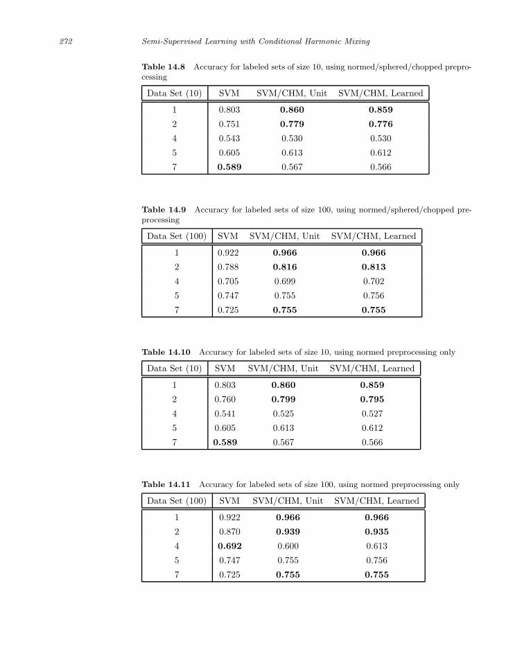
272 Semi-Supervised Learning with Conditional Harmonic Mixing
Table 14.8 Accuracy for labeled sets of size 10, using normed/sphered/chopped prepro-cessing
Data Set (10) SVM SVM/CHM, Unit SVM/CHM, Learned
1 0.803 0.860 0.859
2 0.751 0.779 0.776
4 0.543 0.530 0.530
5 0.605 0.613 0.612
7 0.589 0.567 0.566
Table 14.9 Accuracy for labeled sets of size 100, using normed/sphered/chopped pre-processing
Data Set (100) SVM SVM/CHM, Unit SVM/CHM, Learned
1 0.922 0.966 0.966
2 0.788 0.816 0.813
4 0.705 0.699 0.702
5 0.747 0.755 0.756
7 0.725 0.755 0.755
Table 14.10 Accuracy for labeled sets of size 10, using normed preprocessing only
Data Set (10) SVM SVM/CHM, Unit SVM/CHM, Learned
1 0.803 0.860 0.859
2 0.760 0.799 0.795
4 0.541 0.525 0.527
5 0.605 0.613 0.612
7 0.589 0.567 0.566
Table 14.11 Accuracy for labeled sets of size 100, using normed preprocessing only
Data Set (100) SVM SVM/CHM, Unit SVM/CHM, Learned
1 0.922 0.966 0.966
2 0.870 0.939 0.935
4 0.692 0.600 0.613
5 0.747 0.755 0.756
7 0.725 0.755 0.755

14.8 Conclusions 273
it would be useful to explore more sophisticated methods, for example, methods
that compute a local metric (see, for example, (Xing et al., 2003)). Other techniques
for choosing the conditionals, for example using leave-one-out on the labeled set, or
using a subgraph that is close to the labeled data, may also be fruitful to explore.
14.8 Conclusions
We have presented conditional harmonic mixing (CHM), a graphical model that
can be used for semi-supervised learning. CHM combines and improves upon ear-
lier work in semi-supervised learning in several ways. First, unlike Bayes networks,
CHM can model and learn using conditional probability distributions that do not
have a consistent joint. This freedom allows us to learn and infer using simple lin-
ear algebra. Second, unlike Laplacian SSL, CHM can model asymmetric influences
between random variables. Indeed, our random variables can have different cardinal-
ities: CHM is not limited to simply modeling harmonic functions. Finally, CHM can
use a purely inductive algorithm to provide prior knowledge to the semi-supervised
learning, which leads to superior performance on one-sided and two-sided empir-
ical benchmarks. As the experiments show, one key open question for research is
how to construct graphs that can take full advantage of semi-supervised learning
with CHM: for a given data set, for some choice of graphs the improvement is
significant, while for other choices of graph for the same data set, applying CHM
can even reduce accuracy. This was addressed in the present work by simply using
model averaging over graphs; it seems likely that better methods are possible.
Acknowledgments
We thank David Heckerman and Chris Meek for useful discussions.


IV Change of Representation


15 Graph Kernels by Spectral Transforms
Xiaojin Zhu [email protected]
Jaz Kandola [email protected]
John Lafferty [email protected]
Zoubin Ghahramani [email protected]
Many graph-based semi-supervised learning methods can be viewed as imposing
smoothness conditions on the target function with respect to a graph representing
the data points to be labeled. The smoothness properties of the functions are
encoded in terms of Mercer kernels over the graph. The central quantity in such
regularization is the spectral decomposition of the graph Laplacian, a matrix derived
from the graph’s edge weights. The eigenvectors with small eigenvalues are smooth,
and ideally represent large cluster structures within the data. The eigenvectors
having large eigenvalues are rugged, and considered noise.
Different weightings of the eigenvectors of the graph Laplacian lead to different
measures of smoothness. Such weightings can be viewed as spectral transforms,
that is, as transformations of the standard eigenspectrum that lead to different
regularizers over the graph. Familiar kernels, such as the diffusion kernel resulting
by solving a discrete heat equation on the graph, can be seen as simple parametric
spectral transforms.
The question naturally arises whether one can obtain effective spectral trans-
forms automatically. In this chapter we develop an approach to searching over a
nonparametric family of spectral transforms by using convex optimization to maxi-
mize kernel alignment to the labeled data. Order constraints are imposed to encode
a preference for smoothness with respect to the graph structure. This results in a
flexible family of kernels that is more data-driven than the standard parametric
spectral transforms. Our approach relies on a quadratically constrained quadratic
program (QCQP), and is computationally practical for large data sets.

278 Graph Kernels by Spectral Transforms
15.1 The Graph Laplacian
We are given a labeled data set of input-output pairs (Xl, Yl) = (x1, y1), . . . , (xl, yl)and an unlabeled data set Xu = xl+1, . . . , xn. We form a graph g = (V, E) where
the vertices V are x1, . . . , xn, and the edges E are represented by an n × n ma-
trix W . Entry Wij is the edge weight between nodes i, j, with Wij = 0 if i, j
are not connected. The entries of W have to be non-negative and symmetric,
but it is not necessary for W itself to be positive semi-definite. Let D be the
diagonal degree matrix with Dii =∑
j Wij being the total weight on edges con-
nected to node i. The combinatorial graph Laplacian is defined as L = D − W ,graph Laplacian
which is also called the unnormalized Laplacian. The normalized graph Laplacian
is L = D−1/2LD−1/2 = I − D−1/2WD−1/2.
In graph-based semi-supervised learning the Laplacian L (or L) is a central
object. Let us denote the eigenvalues of L by λ1 ≤ . . . ≤ λn, and the complete
orthonormal set of eigenvectors by φ1 . . . φn. Therefore the spectral decomposition
of the Laplacian is given as L =∑n
i=1 λiφiφ⊤i . We refer readers to (Chung, 1997)spectral
decomposition for a discussion of the mathematical aspects of this decomposition, but briefly
summarize two relevant properties:
Theorem 15.1 The Laplacian L is positive semi-definite, i.e., λi ≥ 0.
Indeed, it is not hard to show that for any function f : [n] → R,
f⊤Lf =1
2
∑
i,j
Wij (f(i) − f(j))2 ≥ 0, (15.1)
where the inequality holds because W has non-negative entries.
Eq. (15.1) measures the smoothness of f on the graph.1 Roughly speaking, f issmoothness of f
smooth if f(i) ≈ f(j) for those pairs with large Wij . This is sometimes informally
expressed by saying that f varies slowly over the graph, or that f follows the data
manifold. In particular, the smoothness of an eigenvector is
φ⊤i Lφi = λi. (15.2)
Thus, eigenvectors with smaller eigenvalues are smoother. Since φi forms a basis
on Rn, we can always write any function f as
f =n∑
i=1
αiφi , αi ∈ R (15.3)
and Eq. 15.1 which measures the smoothness of f can be re-expressed as
f⊤Lf =
n∑
i=1
α2i λi. (15.4)
1. Note that a smaller value means smoother f .

15.1 The Graph Laplacian 279
For semi-supervised learning a smooth function f is part of what we seek, because
this is the prior knowledge encoded by the graph—but we also require that the
function f fits the labels Yl on the inputs Xl.
Theorem 15.2 The graph g has k connected components if and only if λi = 0 for
i = 1, 2, . . . , k.
The corresponding eigenvectors φ1, . . . , φk of L are constant on the nodes within
the corresponding connected component, and zero elsewhere. Note λ1 is always 0
for any graph (Chung, 1997). We will make use of this property later.
(a) a linear unweighted graph with two segments
λ1=0.00 λ
2=0.00 λ
3=0.04 λ
4=0.17 λ
5=0.38
λ6=0.38 λ
7=0.66 λ
8=1.00 λ
9=1.38 λ
10=1.38
λ11
=1.79 λ12
=2.21 λ13
=2.62 λ14
=2.62 λ15
=3.00
λ16
=3.34 λ17
=3.62 λ18
=3.62 λ19
=3.83 λ20
=3.96
(b) the eigenvectors and eigenvalues of the Laplacian L
Figure 15.1 A simple graph and its Laplacian spectral decomposition. Note the eigen-vectors become rougher with larger eigenvalues.
As an example, figure 15.1(a) shows an unweighted graph (Wij = 1 if there is an
edge) consisting of two linear segments. The spectral decomposition of its Laplacian
L is shown in (b). Note that the eigenvectors do indeed look smoother for small λi,
and that the graph has two connected components.

280 Graph Kernels by Spectral Transforms
15.2 Kernels by Spectral Transforms
Kernel methods are increasingly being used for classification because of their
conceptual simplicity, theoretical properties, and good performance on many tasks.
It is attractive to create kernels specifically for semi-supervised learning. We restrict
ourselves to transduction, i.e., the unlabeled data Xu are also the test data. As a
result we only need to consider kernel matrices K ∈ Rn×n on nodes 1, . . . , n in the
graph.
In particular, we want K to respect the smoothness preferences encoded in a
graph. That is, as a regularizer the kernel should penalize functions that are not
smooth over the graph. To establish a link to the graph, we consider K having the
form
K =n∑
i=1
μiφiφ⊤i , (15.5)
where φ are the eigenvectors of the graph Laplacian L, and μi ≥ 0 are the
eigenvalues of K. Since K is the non-negative sum of outer products, it is positive
semi-definite, i.e., a kernel matrix.
The matrix K defines a reproducing kernel Hilbert space (RKHS) with norm
‖f‖2K = 〈f, f〉K =
n∑
i=1
α2i
μi(15.6)
for a function f =∑n
i=1 αiφi. Note if some μi = 0 the corresponding dimension is
not present in the RKHS, and we might define 10 = 0 here.
In many learning algorithms, regularization is expressed as an increasing function
of ‖f‖K . From a semi-supervised learning point of view, we want f to be penalized
if it is not smooth with respect to the graph. Comparing the smoothness of f in
Eq. 15.4 with Eq. 15.6, we find this can be achieved by making μi small if the
Laplacian eigenvalue λi is large, and vice versa.
Indeed, Chapelle et al. (2003) and Smola and Kondor (2003) both suggest a
general principle for creating a semi-supervised kernel K from the graph Laplacian.
Define a spectral transformation function r : R+ → R+ that is non-negative andspectral
transformation decreasing. Set the kernel spectrum by μi = r(λi) to obtain the kernel
K =
n∑
i=1
r(λi)φiφ⊤i . (15.7)
Note that r essentially reverses the order of the eigenvalues, so that smooth φi’s
have larger eigenvalues in K. Since r is decreasing, a greater penalty is incurred if
a function is not smooth.
The transform r is often chosen from a parametric family, resulting in some
familiar kernels. For example Chapelle et al. (2003) and Smola and Kondor (2003)
list the following transformations on L:

15.3 Kernel Alignment 281
regularized Laplacian: r(λ) = 1λ+ǫ
diffusion kernel: r(λ) = exp(−σ2
2 λ)
one-step random walk: r(λ) = (α − λ) with α ≥ 2
p-step random walk: r(λ) = (α − λ)p with α ≥ 2
inverse cosine: r(λ) = cos(λπ/4)
step function: r(λ) = 1 if λ ≤ λcut
Each has its own special interpretation. The regularized Laplacian is also known
as the Gaussian field kernel (Zhu et al., 2003c). Of course there are many other
natural choices for r. Although the general principle of Eq. 15.7 is appealing, it
does not address the question of which parametric family to use. Moreover, the
hyperparameters (e.g., σ or ǫ above) in a particular parametric family may not suit
the task at hand, resulting in overly constrained kernels.
Is there an optimal spectral transformation? The following sections address
this question. The short answer is yes, in a certain sense. We select a spectral
transformation that optimizes kernel alignment to the labeled data, while imposing
an ordering constraint but otherwise not assuming any parametric form. Kernel
alignment is a surrogate for classification accuracy, and, importantly, leads to a
convex optimization problem.
15.3 Kernel Alignment
The empirical kernel alignment (Cristianini et al., 2002a; Lanckriet et al., 2004a)
assesses the fitness of a kernel to training labels. The alignment has a number
of convenient properties: it can be efficiently computed before any training of
the kernel machine takes place, and based only on training data information.
The empirical alignment can also be shown to be sharply concentrated around
its expected value, allowing it to be estimated from finite samples. A connection
between high alignment and good generalization performance has been established
in (Cristianini et al., 2002a).
As we will compare matrices, we introduce here the Frobenius product 〈., .〉FFrobenius
product between two square matrices M and N of the same size:
〈M, N〉F =∑
ij
mijnij = Tr(MN).
The empirical kernel alignment compares the l×l kernel matrix Ktr on the labeled
training set x1, . . . , xl, and a target matrix T derived from the labels y1, . . . , yl. One
such target matrix is Tij = 1 if yi = yj , and −1 otherwise. Note for binary +1,−1training labels Yl = (y1 . . . yl)
⊤ this is simply the rank one matrix T = YlYl⊤. The
empirical kernel alignment is defined as follows.
Definition 15.3 (empirical kernel alignment) Let Ktr be the kernel matrix

282 Graph Kernels by Spectral Transforms
restricted to the training points, and T the target matrix on training data. We
define the empirical kernel alignment asempirical kernel
alignmentA(Ktr, T ) =
〈Ktr, T 〉F√〈Ktr, Ktr〉F 〈T, T 〉F
. (15.8)
The empirical alignment is essentially the cosine between the matrices Ktr and
T . The range of the alignment is [0, 1]. The larger its value the closer is the kernel
to the target. This quantity is maximized when Ktr ∝ T .
15.4 Optimizing Alignment Using QCQP for Semi-Supervised Learning
Having introduced the alignment quantity, now let us consider the problem of semi-
supervised kernel construction using a principled nonparametric approach. In short,
we will learn the spectral transformation μi ≡ r(λi) (15.7) by optimizing the
resulting kernel alignment, with certain restrictions. Notice we no longer assume
a parametric function r(); instead we work with the transformed eigenvalues μi’s
directly.
When the kernel matrix is defined as K =∑n
i=1 μiφiφi⊤ and the target T
given, the kernel alignment between the labeled submatrix Ktr and T is a convex
function in μi’s. Nonetheless, in general we have to make sure K is a valid kernel
matrix, i.e., it is positive semi-definite. This is a semi-definite program (SDP),
which has high computational complexity (Boyd and Vandenberghe, 2004). We thus
restrict μi ≥ 0, ∀i. This guarantees K to be positive semi-definite, and reduces the
optimization problem into a quadratically constrained quadratic program (QCQP),
which is computationally more efficient. In a QCQP both the objective functionquadratically
constrained
quadratic
programs
and the constraints are quadratic, as illustrated below:
minimize1
2x⊤P0x + q⊤0 x + r0 (15.9)
subject to1
2x⊤Pix + q⊤i x + ri ≤ 0 i = 1 · · ·m (15.10)
Ax = b, (15.11)
where Pi ∈ Sn+, i = 0, . . . , m, where Sn
+ defines the set of square symmetric positive
semi-definite matrices. In a QCQP, we minimize a convex quadratic function over
a feasible region that is the intersection of ellipsoids. The number of iterations
required to reach the solution is comparable to the number required for linear
programs, making the approach feasible for large data sets.
Previous work using kernel alignment did not take into account that the “building
blocks” Ki = φiφi⊤ were derived from the graph Laplacian with the goal of semi-
supervised learning. As such, the μi’s can take arbitrary non-negative values and
there is no preference to penalize components that do not vary smoothly over the
graph. This shall be rectified by requiring smoother eigenvectors to receive larger
coefficients, as shown in the next section.

15.5 Semi-Supervised Kernels with Order Constraints 283
15.5 Semi-Supervised Kernels with Order Constraints
We would like to maintain a decreasing order on the spectral transformation μi
to reflect the prior knowledge encoded in the graph, that smooth functions are
preferred. This motivates the set of order constraints:order constraints
μi ≥ μi+1, i = 1 · · ·n − 1. (15.12)
And we can specify the desired semi-supervised kernel as follows:
Definition 15.4 (order-constrained kernel) An order-constrained semi-supervisedorder-constrained
kernel kernel K is the solution to the following convex optimization problem:
maxK A(Ktr, T ) (15.13)
subject to K =∑n
i=1 μiKi (15.14)
μi ≥ 0 (15.15)
Tr(K) = 1 (15.16)
μi ≥ μi+1, i = 1 · · ·n − 1, (15.17)
where T is the training target matrix, Ki = φiφ⊤i and φi’s are the eigenvectors of
the graph Laplacian.
This formulation is an extension of the original kernel alignment of Lanckriet et al.
(2004a), with the addition of order constraints, and with special components Ki’s
from the graph Laplacian. Since μi ≥ 0 and Ki’s are outer products, K will
automatically be positive semi-definite and hence a valid kernel matrix. The trace
constraint is needed to fix the scale invariance of kernel alignment. It is important
to notice the order constraints are convex and as such, definition 15.4 is a convex
optimization problem.convex
optimization The problem is equivalent to
maxK 〈Ktr, T 〉F (15.18)
subject to 〈Ktr, Ktr〉F ≤ 1 (15.19)
K =∑n
i=1 μiKi (15.20)
μi ≥ 0 (15.21)
μi ≥ μi+1, i = 1 · · ·n − 1, (15.22)
where the trace constraint is replaced by (15.19) (up to a constant factor). Let
vec(A) be the column vectorization of a matrix A. Defining
M =[vec(K1,tr) · · · vec(Km,tr)
](15.23)

284 Graph Kernels by Spectral Transforms
it is not hard to show that the problem can then be expressed as
maxμ vec(T )⊤Mμ (15.24)
subject to ||Mμ|| ≤ 1 (15.25)
μi ≥ 0 (15.26)
μi ≥ μi+1, i = 1 · · ·n − 1. (15.27)
The objective function is linear in μ, and there is a simple cone constraint, making
it a QCQP.
We can further improve the kernel. Consider a graph that has a single connected
component, i.e., any node can reach any other node via one or more edges. Such
graphs are common in practice. By the basic property of the Laplacian we know
λ1 = 0, and the corresponding eigenvector φi is a constant. Therefore K1 = φiφ⊤i is
a constant matrix. Such a constant matrix acts as a bias term in the graph kernel,bias term
as in (15.7). We should not constrain μ1 as in definition 15.4, but allow the bias of
the kernel to vary freely. This motivates the following definition:
Definition 15.5 (improved order-constrained kernel) An improved order-constrainedimproved
order-constrained
kernel
semi-supervised kernel K is the solution to the same problem in definition 15.4, but
the order constraints (15.17) apply only to nonconstant eigenvectors:
μi ≥ μi+1, i = 1 · · ·n − 1, and φi not constant. (15.28)
It should be pointed out that the improved order-constrained kernel is identical
to the order-constrained kernel when the graph has disjoint components. This is
because the first k eigenvectors are piecewise constant over the components, but
not constant overall, when the graph has k > 1 connected components. We in
fact would like to emphasize these eigenvectors because they might correspond to
natural clusters in data. Thus we will still enforce the order constraints on them.
The definition in (15.28) is meant to target μ1 in connected graphs only. As discussed
above, in this situation μ1 is the bias term of the kernel. The only “improvement” in
the improved order-constrained kernel is that we do not constrain such bias terms.
As the experiments show later, this improves the quality of the kernels markedly.
In practice we do not need all n eigenvectors of the graph Laplacian, or equiva-
lently all n Ki’s. The first m < n eigenvectors with the smallest eigenvalues work
well empirically. Also note we could have used the fact that Ki’s are from orthog-
onal eigenvectors φi to further simplify the expression. However, we leave it as is,
making it easier to incorporate other kernel components if necessary.
It is illustrative to compare and contrast the order-constrained semi-supervised
kernels to other related kernels. We call the original kernel alignment solution in
(Lanckriet et al., 2004a) a maximal-alignment kernel. It is the solution to defi-maximal-
alignment
kernel
nition 15.4 without the order constraints (15.17). Because it does not have the
additional constraints, it maximizes kernel alignment among all spectral transfor-
mations. The hyperparameters σ and ǫ of the diffusion kernel and Gaussian field
kernel (described in section 15.2) can be learned by maximizing the alignment score

15.6 Experimental Results 285
also, although the optimization problem is not necessarily convex. These kernels
use different information from the original Laplacian eigenvalues λi. The maximal-different
information usage alignment kernels ignore λi altogether. The order-constrained semi-supervised ker-
nels only use the order of λi and ignore their actual values. The diffusion and
Gaussian field kernels use the actual values. In terms of the degrees of freedom in
choosing the spectral transformation μi’s, the maximal-alignment kernels are com-
pletely free. The diffusion and Gaussian field kernels are restrictive since they have
an implicit parametric form and only one free parameter. The order-constrained
semi-supervised kernels incorporate desirable features from both approaches.
15.6 Experimental Results
We evaluate kernels on seven data sets. The data sets and the corresponding graphs
are summarized in table 15.1. baseball-hockey, pc-mac and religion-atheism are
binary document categorization tasks taken from the 20-newsgroups data set. The
distance measure is the cosine similarity between tf.idf vectors. one-two, odd-even,
and ten digits are handwritten digits recognition tasks originally from the Cedar
Buffalo binary digits database. one-two is digits “1” versus “2”; odd-even is the
artificial task of classifying odd “1, 3, 5, 7, 9” versus even “0, 2, 4, 6, 8” digits,
such that each class has several well-defined internal clusters; ten digits is 10-way
classification; isolet is isolated spoken English alphabet recognition from the UCI
repository. For these data sets we use Euclidean distance on raw features. We use
10-nearest-neighbor (10NN) unweighted graphs on all data sets except isolet which
is 100NN. For all data sets, we use the smallest m = 200 eigenvalue and eigenvector
pairs from the graph Laplacian. These values are set arbitrarily without optimizing
and do not create an unfair advantage to the order-constrained kernels. For each
data set we test on five different labeled set sizes. For a given labeled set size, we
perform 30 random trials in which a labeled set is randomly sampled from the
whole data set. All classes must be present in the labeled set. The rest is used as
an unlabeled (test) set in that trial.
We compare a total of eight different types of kernels. Five are semi-supervised
kernels: improved order-constrained kernels, order-constrained kernels, Gaussian
field kernels (section 15.2), diffusion kernels (section 15.2), and maximal-alignment
kernels (section 15.5). Three are standard supervised kernels, which do not use
unlabeled data in kernel construction: linear kernels, quadratic kernels, and radial
basis function (RBF) kernels.
We compute the spectral transformation for improved order-constrained kernels,
order-constrained kernels, and maximal-alignment kernels by solving the QCQP
using the standard solver SeDuMi/YALMIP (see (Sturm, 1999) and (Lofberg,
2004)). The hyperparameters in the Gaussian field kernels and diffusion kernels
are learned with the fminbnd() function in Matlab to maximize kernel alignment.
The bandwidth of the RBF kernels are learned using fivefold cross-validation on
labeled set accuracy. Here and below we use cross-validation – it is done independent

286 Graph Kernels by Spectral Transforms
Table 15.1 Summary of data sets
data set instances classes graph
baseball-hockey 1993 2 cosine similarity 10NN unweighted
pc-mac 1943 2 cosine similarity 10NN unweighted
religion-atheism 1427 2 cosine similarity 10NN unweighted
one-two 2200 2 Euclidean 10NN unweighted
odd-even 4000 2 Euclidean 10NN unweighted
ten digits 4000 10 Euclidean 10NN unweighted
isolet 7797 26 Euclidean 100NN unweighted
of and after kernel alignment methods, to optimize a quantity not related to the
proposed kernels.
We apply the eight kernels to the same support vector machine (SVM) in order
to compute the accuracy on unlabeled data. For each task and kernel combination,
we choose the bound on SVM slack variables C with fivefold cross-validation on
labeled set accuracy. For multiclass classification we perform one-against-all and
pick the class with the largest margin.
Table 15.2 Baseball vs. hockey
semi-supervised kernels standard kernels
Training Improved Order Gaussian Diffusion Max-align RBF Linear Quadratic
set size Order Field σ = 200
10 95.7±8.9 93.9±12.0 63.1±15.8 65.8±22.8 93.2±6.8 53.6±5.5 68.1±7.6 68.1±7.6
0.90 ( 2) 0.69 ( 1) 0.35 0.44 0.95 ( 1) 0.11 0.29 0.23
30 98.0±0.2 97.3±2.1 91.8±9.3 59.1±17.9 96.6±2.2 69.3±11.2 78.5±8.5 77.8±10.6
0.91 ( 9) 0.67 ( 9) 0.25 0.39 0.93 ( 6) 0.03 0.17 0.11
50 97.9±0.5 97.8±0.6 96.7±0.6 93.7±6.8 97.0±1.1 77.7±8.3 84.1±7.8 75.6±14.2
0.89 (29) 0.63 (29) 0.22 0.36 0.90 (27) 0.02 0.15 0.09
70 97.9±0.3 97.9±0.3 96.8±0.6 97.5±1.4 97.2±0.8 83.9±7.2 87.5±6.5 76.1±14.9
0.90 (68) 0.64 (64) 0.22 0.37 0.90 (46) 0.01 0.13 0.07
90 98.0±0.5 98.0±0.2 97.0±0.4 97.8±0.2 97.6±0.3 88.5±5.1 89.3±4.4 73.3±16.8
0.89 (103) 0.63 (101) 0.21 0.36 0.89 (90) 0.01 0.12 0.06
Tables 15.2 through 15.8 list the results. There are two rows for each cell:
the upper row is the average test (unlabeled) set accuracy with one standard
deviation; the lower row is the average training (labeled) set kernel alignment,
and in parenthesis the average run time in seconds for QCQP on a 2.4GHz Linux
computer. Each number is averaged over 30 random trials. To assess the statistical
significance of the results, we perform paired t-test on test accuracy. We highlight
the best accuracy in each row, and those that cannot be distinguished from the
best with paired t-test at significance level 0.05.
We find that:
The five semi-supervised kernels tend to outperform the three standard supervised

15.6 Experimental Results 287
Table 15.3 PC vs. MAC
semi-supervised kernels standard kernels
Training Improved Order Gaussian Diffusion Max-align RBF Linear Quadratic
set size Order Field σ = 100
10 87.0±5.0 84.9±7.2 56.4±6.2 57.8±11.5 71.1±9.7 51.6±3.4 63.0±5.1 62.3±4.2
0.71 ( 1) 0.57 ( 1) 0.32 0.35 0.90 ( 1) 0.11 0.30 0.25
30 90.3±1.3 89.6±2.3 76.4±6.1 79.6±11.2 85.4±3.9 62.6±9.6 71.8±5.5 71.2±5.3
0.68 ( 8) 0.49 ( 8) 0.19 0.23 0.74 ( 6) 0.03 0.18 0.13
50 91.3±0.9 90.5±1.7 81.1±4.6 87.5±2.8 88.4±2.1 67.8±9.0 77.6±4.8 75.7±5.4
0.64 (31) 0.46 (31) 0.16 0.20 0.68 (25) 0.02 0.14 0.10
70 91.5±0.6 90.8±1.3 84.6±2.1 90.5±1.2 89.6±1.6 74.7±7.4 80.2±4.6 74.3±8.7
0.63 (70) 0.46 (56) 0.14 0.19 0.66 (59) 0.01 0.12 0.08
90 91.5±0.6 91.3±1.3 86.3±2.3 91.3±1.1 90.3±1.0 79.0±6.4 82.5±4.2 79.1±7.3
0.63 (108) 0.45 (98) 0.13 0.18 0.65 (84) 0.01 0.11 0.08
Table 15.4 Religion vs. atheism
semi-supervised kernels standard kernels
Training Improved Order Gaussian Diffusion Max-align RBF Linear Quadratic
set size Order Field σ = 130
10 72.8±11.2 70.9±10.9 55.2±5.8 60.9±10.7 60.7±7.5 55.8±5.8 60.1±7.0 61.2±4.8
0.50 ( 1) 0.42 ( 1) 0.31 0.31 0.85 ( 1) 0.13 0.30 0.26
30 84.2±2.4 83.0±2.9 71.2±6.3 80.3±5.1 74.4±5.4 63.4±6.5 63.7±8.3 70.1±6.3
0.38 ( 8) 0.31 ( 6) 0.20 0.22 0.60 ( 7) 0.05 0.18 0.15
50 84.5±2.3 83.5±2.5 80.4±4.1 83.5±2.7 77.4±6.1 69.3±6.5 69.4±7.0 70.7±8.5
0.31 (28) 0.26 (23) 0.17 0.20 0.48 (27) 0.04 0.15 0.11
70 85.7±1.4 85.3±1.6 83.0±2.9 85.4±1.8 82.3±3.0 73.1±5.8 75.7±6.0 71.0±10.0
0.29 (55) 0.25 (42) 0.16 0.19 0.43 (51) 0.03 0.13 0.10
90 86.6±1.3 86.4±1.5 84.5±2.1 86.2±1.6 82.8±2.6 77.7±5.1 74.6±7.6 70.0±11.5
0.27 (86) 0.24 (92) 0.15 0.18 0.40 (85) 0.02 0.12 0.09
Table 15.5 One vs. two
semi-supervised kernels standard kernels
Training Improved Order Gaussian Diffusion Max-align RBF Linear Quadratic
set size Order Field σ = 1000
10 96.2±2.7 90.6±14.0 58.2±17.6 59.4±18.9 85.4±11.5 78.7±14.3 85.1±5.7 85.7±4.8
0.87 ( 2) 0.66 ( 1) 0.43 0.53 0.95 ( 1) 0.38 0.26 0.30
20 96.4±2.8 93.9±8.7 87.0±16.0 83.2±19.8 94.5±1.6 90.4±4.6 86.0±9.4 90.9±3.7
0.87 ( 3) 0.64 ( 4) 0.38 0.50 0.90 ( 3) 0.33 0.22 0.25
30 98.2±2.1 97.2±2.5 98.1±2.2 98.1±2.7 96.4±2.1 93.6±3.1 89.6±5.9 92.9±2.8
0.84 ( 8) 0.61 ( 7) 0.35 0.47 0.86 ( 6) 0.30 0.17 0.24
40 98.3±1.9 96.5±2.4 98.9±1.8 99.1±1.4 96.3±2.3 94.0±2.7 91.6±6.3 94.9±2.0
0.84 (13) 0.61 (15) 0.36 0.48 0.86 (11) 0.29 0.18 0.21
50 98.4±1.9 95.6±9.0 99.4±0.5 99.6±0.3 96.6±2.3 96.1±2.4 93.0±3.6 95.8±2.3
0.83 (31) 0.60 (37) 0.35 0.46 0.84 (25) 0.28 0.17 0.20

288 Graph Kernels by Spectral Transforms
Table 15.6 Odd vs. even
semi-supervised kernels standard kernels
Training Improved Order Gaussian Diffusion Max-align RBF Linear Quadratic
set size Order Field σ = 1500
10 69.6±6.5 68.8±6.1 65.5±8.9 68.4±8.5 55.7±4.4 65.0±7.0 63.1±6.9 65.4±6.5
0.45 ( 1) 0.41 ( 1) 0.32 0.34 0.86 ( 1) 0.23 0.25 0.27
30 82.4±4.1 82.0±4.0 79.6±4.1 83.0±4.2 67.2±5.0 77.7±3.5 72.4±6.1 76.5±5.1
0.32 ( 6) 0.28 ( 6) 0.21 0.23 0.56 ( 6) 0.10 0.11 0.16
50 87.6±3.5 87.5±3.4 85.9±3.8 89.1±2.7 76.0±5.3 81.8±2.7 74.4±9.2 81.3±3.1
0.29 (24) 0.26 (25) 0.19 0.21 0.45 (26) 0.07 0.09 0.12
70 89.2±2.6 89.0±2.7 89.0±1.9 90.3±2.8 80.9±4.4 84.4±2.0 73.6±10.0 83.8±2.8
0.27 (65) 0.24 (50) 0.17 0.20 0.39 (51) 0.06 0.07 0.12
90 91.5±1.5 91.4±1.6 90.5±1.4 91.9±1.7 85.4±3.1 86.1±1.8 66.1±14.8 85.5±1.6
0.26 (94) 0.23 (97) 0.16 0.19 0.36 (88) 0.05 0.07 0.11
Table 15.7 Ten digits (10 classes)
semi-supervised kernels standard kernels
Training Improved Order Gaussian Diffusion Max-align RBF Linear Quadratic
set size Order Field σ = 2000
50 76.6±4.3 71.5±5.0 41.4±6.8 49.8±6.3 70.3±5.2 57.0±4.0 50.2±9.0 66.3±3.7
0.47 (26) 0.21 (26) 0.15 0.16 0.51 (25) -0.62 -0.50 -0.25
100 84.8±2.6 83.4±2.6 63.7±3.5 72.5±3.3 80.7±2.6 69.4±1.9 56.0±7.8 77.2±2.3
0.47 (124) 0.17 (98) 0.12 0.13 0.49 (100) -0.64 -0.52 -0.29
150 86.5±1.7 86.4±1.3 75.1±3.0 80.4±2.1 84.5±1.9 75.2±1.4 56.2±7.2 81.4±2.2
0.48 (310) 0.18 (255) 0.11 0.13 0.50 (244) -0.66 -0.53 -0.31
200 88.1±1.3 88.0±1.3 80.4±2.5 84.4±1.6 86.0±1.5 78.3±1.3 60.8±7.3 84.3±1.7
0.47 (708) 0.16 (477) 0.10 0.11 0.49 (523) -0.65 -0.54 -0.33
250 89.1±1.1 89.3±1.0 84.6±1.4 87.2±1.3 87.2±1.3 80.4±1.4 61.3±7.6 85.7±1.3
0.47 (942) 0.16 (873) 0.10 0.11 0.49 (706) -0.65 -0.54 -0.33
Table 15.8 Isolet (26 classes)
semi-supervised kernels standard kernels
Training Improved Order Gaussian Diffusion Max-align RBF Linear Quadratic
set size Order Field σ = 30
50 56.0±3.5 42.0±5.2 41.2±2.9 29.0±2.7 50.1±3.7 28.7±2.0 30.0±2.7 23.7±2.4
0.27 (26) 0.13 (25) 0.03 0.11 0.31 (24) -0.89 -0.80 -0.65
100 64.6±2.1 59.0±3.6 58.5±2.9 47.4±2.7 63.2±1.9 46.3±2.4 46.6±2.7 42.0±2.9
0.26 (105) 0.10 (127) -0.02 0.08 0.29 (102) -0.90 -0.82 -0.69
150 67.6±2.6 65.2±3.0 65.4±2.6 57.2±2.7 67.9±2.5 57.6±1.5 57.3±1.8 53.8±2.2
0.26 (249) 0.09 (280) -0.05 0.07 0.27 (221) -0.90 -0.83 -0.70
200 71.0±1.8 70.9±2.3 70.6±1.9 64.8±2.1 72.3±1.7 63.9±1.6 64.2±2.0 60.5±1.6
0.26 (441) 0.08 (570) -0.07 0.06 0.27 (423) -0.91 -0.83 -0.72
250 71.8±2.3 73.6±1.5 73.7±1.2 69.8±1.5 74.2±1.5 68.8±1.5 69.5±1.7 66.2±1.4
0.26 (709) 0.08 (836) -0.07 0.06 0.27 (665) -0.91 -0.84 -0.72

15.7 Conclusion 289
kernels. It shows that with properly constructed graphs, unlabeled data can help
classification.
The order-constrained kernel is often quite good, but the improved order-
constrained kernel is even better. All the graphs on these data sets happen to
be connected. Recall this is when the improved order-constrained kernel differs
from the order-constrained kernel by not constraining the bias term. Obviously a
flexible bias term is important for classification accuracy.
Figure 15.2 shows the spectral transformation μi of the five semi-supervised
kernels for different tasks. These are the average of the 30 trials with the largest
labeled set size in each task. The x-axis is in increasing order of λi (the original
eigenvalues of the Laplacian). The mean (thick lines) and ±1 standard deviation
(dotted lines) of only the top 50 μi’s are plotted for clarity. The μi values are scaled
vertically for easy comparison among kernels. As expected the maximal-alignment
kernels’ spectral transformation is zigzagged, diffusion’s and Gaussian field’s are
very smooth, while (improved) order-constrained kernels are in between.
The order-constrained kernels (green) have large μ1 because of the order con-
straint on the constant eigenvector. Again this seems to be disadvantageous — the
spectral transformation tries to balance it out by increasing the value of other μi’s,
so that the bias term K1’s relative influence is smaller. On the other hand, the
improved order-constrained kernels (black) allow μ1 to be small. As a result the
rest μi’s decay fast, which is desirable.
In summary, the improved order-constrained kernel is consistently the best among
all kernels.
15.7 Conclusion
We have proposed and evaluated a novel approach for semi-supervised kernel
construction using convex optimization. The method incorporates order constraints,
and the resulting convex optimization problem can be solved efficiently using a
QCQP. In this work the base kernels were derived from the graph Laplacian, and no
parametric form for the spectral transformation was imposed, making the approach
more general than previous approaches. Experiments show that the method is both
computationally feasible and results in improvements in classification performance
when used with support vector machines.
There are several future directions:
In both order-constrained kernels and improved order-constrained kernels, we
are learning a large number of parameters μ1, . . . , μn based on l labeled examples.
Usually l ≪ n, which suggests the danger of overfitting. However, we have to
consider two mitigating factors: the first is that we in practice only learn the
top m < n parameters and set the rest at zero; the second is that the μ’s are
order-constrained, which reduces the effective complexity. One interesting question

290 Graph Kernels by Spectral Transforms
0 10 20 30 40 500
0.2
0.4
0.6
0.8
1
rank
µ s
cale
d
Baseball vs. Hockey
Improved orderOrderMaxalignGaussian fieldDiffusion
0 10 20 30 40 500
0.2
0.4
0.6
0.8
1
rank
µ s
cale
d
PC vs. MAC
Improved orderOrderMaxalignGaussian fieldDiffusion
0 10 20 30 40 500
0.2
0.4
0.6
0.8
1
rank
µ s
cale
d
Religion vs. Atheism
Improved orderOrderMaxalignGaussian fieldDiffusion
0 10 20 30 40 500
0.2
0.4
0.6
0.8
1
rank
µ s
cale
d
One vs. Two
Improved orderOrderMaxalignGaussian fieldDiffusion
0 10 20 30 40 500
0.2
0.4
0.6
0.8
1
rank
µ s
cale
d
Odd vs. Even
Improved orderOrderMaxalignGaussian fieldDiffusion
0 10 20 30 40 500
0.2
0.4
0.6
0.8
1
rank
µ s
cale
dTen Digits (10 classes)
Improved orderOrderMaxalignGaussian fieldDiffusion
0 10 20 30 40 500
0.2
0.4
0.6
0.8
1
rank
µ s
cale
d
ISOLET (26 classes)
Improved orderOrderMaxalignGaussian fieldDiffusion
Figure 15.2 Comparison of spectral transformation for the five semi-supervised kernels.

15.7 Conclusion 291
for future research is an estimate of the effective number of parameters in these
methods.
The QCQP problem may be transformed into a standard quadratic program
(QP), which may result in further improvements in computational efficiency.
The alignment is one example of a cost function that can be optimized. With
a fixed kernel, margin-based upper bounds on misclassification probability can be
derived. As such, other cost functions that directly optimize quantities such as
the margin can also be used. This approach has been considered in the work of
Chapelle and Vapnik (2000) where the so-called span bound was introduced and
optimized using gradient descent; and in (Lanckriet et al., 2004a; Bousquet and
Herrmann, 2002) where optimization of tighter Rademacher complexity bounds
has been proposed.
Acknowledgment
We thank Olivier Chapelle and the anonymous reviewers for their comments and
suggestions.


16 Spectral Methods for Dimensionality
Reduction
Lawrence K. Saul [email protected]
Kilian Q. Weinberger [email protected]
Fei Sha [email protected]
Jihun Ham [email protected]
Daniel D. Lee [email protected]
How can we search for low-dimensional structure in high-dimensional data? If the
data are mainly confined to a low-dimensional subspace, then simple linear methods
can be used to discover the subspace and estimate its dimensionality. More generally,
though, if the data lie on (or near) a low-dimensional submanifold, then its structure
may be highly nonlinear, and linear methods are bound to fail.
Spectral methods have recently emerged as a powerful tool for nonlinear dimen-
sionality reduction and manifold learning. These methods are able to reveal low-
dimensional structure in high-dimensional data from the top or bottom eigenvectors
of specially constructed matrices. To analyze data that lie on a low-dimensional
submanifold, the matrices are constructed from sparse weighted graphs whose ver-
tices represent input patterns and whose edges indicate neighborhood relations.
The main computations for manifold learning are based on tractable, polynomial-
time optimizations, such as shortest-path problems, least-squares fits, semi-definite
programming, and matrix diagonalization. This chapter provides an overview of
unsupervised learning algorithms that can be viewed as spectral methods for linear
and nonlinear dimensionality reduction.
16.1 Introduction
The problem of dimensionality reduction—extracting low-dimensional structure
from high-dimensional data—arises often in machine learning and statistical patterndimensionality
reduction recognition. High-dimensional data take many different forms: from digital image
libraries to gene expression microarrays, from neuronal population activities to

294 Spectral Methods for Dimensionality Reduction
financial time series. By formulating the problem of dimensionality reduction in a
general setting, however, we can analyze many different types of data in the same
underlying mathematical framework.
We therefore consider the following problem. Given a high-dimensional data
set X = (x1, . . . , xn) of input patterns where xi ∈ Rd, how can we compute n
corresponding output patterns ψi ∈ Rm that provide a faithful low-dimensional
representation of the original data set with m ≪ d? By “faithful,” we meaninputs xi ∈ Rd
outputs ψi ∈ Rm generally that nearby inputs are mapped to nearby outputs, while faraway inputs
are mapped to faraway outputs; we will be more precise in what follows. Ideally,
an unsupervised learning algorithm should also estimate the value of m that is
required for a faithful low-dimensional representation. Without loss of generality,
we assume everywhere in this chapter that the inputs are centered on the origin,
with∑
i xi = 0 ∈ Rd.
This chapter provides a survey of so-called spectral methods for dimensionality
reduction, where the low-dimensional representations are derived from the top
or bottom eigenvectors of specially constructed matrices. The aim is not to bespectral methods
exhaustive, but to describe the simplest forms of a few representative algorithms
using terminology and notation consistent with the other chapters in this book.
At best, we can only hope to provide a snapshot of the rapidly growing literature
on this subject. An excellent and somewhat more detailed survey of many of these
algorithms is given by Burges (2005). In the interests of both brevity and clarity,
the examples of nonlinear dimensionality reduction in this chapter were chosen
specifically for their pedagogical value; more interesting applications to data sets
of images, speech, and text can be found in the original papers describing each
method.
The chapter is organized as follows. In section 16.2, we review the classical meth-
ods of principal component analysis (PCA) and metric multidimensional scaling
(MDS). The outputs returned by these methods are related to the input patterns
by a simple linear transformation. The remainder of the chapter focuses on the more
interesting problem of nonlinear dimensionality reduction. In section 16.3, we de-
scribe several graph-based methods that can be used to analyze high-dimensional
data that have been sampled from a low-dimensional submanifold. All of these
graph-based methods share a similar structure—computing nearest neighbors of
the input patterns, constructing a weighted graph based on these neighborhood re-
lations, deriving a matrix from this weighted graph, and producing an embedding
from the top or bottom eigenvectors of this matrix. Notwithstanding this shared
structure, however, these algorithms are based on rather different geometric in-
tuitions and intermediate computations. In section 16.4, we describe kernel-based
methods for nonlinear dimensionality reduction and show how to interpret graph-
based methods in this framework. Finally, in section 16.5, we conclude by contrast-
ing the properties of different spectral methods and highlighting various ongoing
lines of research. We also point out connections to related work on semi-supervised
learning, as described by other authors in this book.
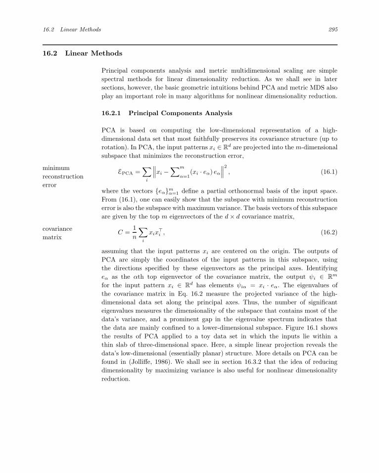
16.2 Linear Methods 295
16.2 Linear Methods
Principal components analysis and metric multidimensional scaling are simple
spectral methods for linear dimensionality reduction. As we shall see in later
sections, however, the basic geometric intuitions behind PCA and metric MDS also
play an important role in many algorithms for nonlinear dimensionality reduction.
16.2.1 Principal Components Analysis
PCA is based on computing the low-dimensional representation of a high-
dimensional data set that most faithfully preserves its covariance structure (up to
rotation). In PCA, the input patterns xi ∈ Rd are projected into the m-dimensional
subspace that minimizes the reconstruction error,
minimum
reconstruction
error
EPCA =∑
i
∥∥∥xi −∑m
α=1(xi · eα) eα
∥∥∥2
, (16.1)
where the vectors eαmα=1 define a partial orthonormal basis of the input space.
From (16.1), one can easily show that the subspace with minimum reconstruction
error is also the subspace with maximum variance. The basis vectors of this subspace
are given by the top m eigenvectors of the d × d covariance matrix,
covariance
matrixC =
1
n
∑
i
xix⊤i , (16.2)
assuming that the input patterns xi are centered on the origin. The outputs of
PCA are simply the coordinates of the input patterns in this subspace, using
the directions specified by these eigenvectors as the principal axes. Identifying
eα as the αth top eigenvector of the covariance matrix, the output ψi ∈ Rm
for the input pattern xi ∈ Rd has elements ψiα = xi · eα. The eigenvalues of
the covariance matrix in Eq. 16.2 measure the projected variance of the high-
dimensional data set along the principal axes. Thus, the number of significant
eigenvalues measures the dimensionality of the subspace that contains most of the
data’s variance, and a prominent gap in the eigenvalue spectrum indicates that
the data are mainly confined to a lower-dimensional subspace. Figure 16.1 shows
the results of PCA applied to a toy data set in which the inputs lie within a
thin slab of three-dimensional space. Here, a simple linear projection reveals the
data’s low-dimensional (essentially planar) structure. More details on PCA can be
found in (Jolliffe, 1986). We shall see in section 16.3.2 that the idea of reducing
dimensionality by maximizing variance is also useful for nonlinear dimensionality
reduction.

296 Spectral Methods for Dimensionality Reduction
Figure 16.1 Results of PCA applied to n = 1600 input patterns in d = 3 dimensionsthat lie within a thin slab. The top two eigenvectors of the covariance matrix, denotedby black arrows, indicate the m = 2 dimensional subspace of maximum variance. Theeigenvalues of the covariance matrix are shown normalized by their sum: each eigenvalueis indicated by a colored bar whose length reflects its partial contribution to the overalltrace of the covariance matrix. There are two dominant eigenvalues, indicating that thedata are very nearly confined to a plane.
16.2.2 Metric Multidimensional Scaling
Metric MDS is based on computing the low-dimensional representation of a high-
dimensional data set that most faithfully preserves the inner products between
different input patterns. The outputs ψi ∈ Rm of metric MDS are chosen to
minimize:
EMDS =∑
ij
(xi · xj − ψi · ψj)2. (16.3)
The minimum error solution is obtained from the spectral decomposition of the
Gram matrix of inner products,
Gram
matrix Gij = xi · xj . (16.4)
Denoting the top m eigenvectors of this Gram matrix by vαmα=1 and their
respective eigenvalues by λαmα=1, the outputs of MDS are given by ψiα =
√λαvαi.
Though MDS is designed to preserve inner products, it is often motivated by
the idea of preserving pairwise distances. Let Sij = ‖xi − xj‖2 denote the matrixdistance
preservation of squared pairwise distances between input patterns. Often the input to MDS
is specified in this form. Assuming that the inputs are centered on the origin,
a Gram matrix consistent with these squared distances can be derived from the
transformation G = − 12 (I − uu⊤)S(I − uu⊤), where I is the n× n identity matrix
and u = 1√n(1, 1, . . . , 1)⊤ is the uniform vector of unit length. More details on MDS
can be found in (Cox and Cox, 1994).
Though based on a somewhat different geometric intuition, metric MDS yields
the same outputs ψi ∈ Rm as PCA—essentially a rotation of the inputs followed
by a projection into the subspace with the highest variance. (The outputs of both
algorithms are invariant to global rotations of the input patterns.) The Gram matrix
of metric MDS has the same rank and eigenvalues up to a constant factor as the

16.3 Graph-Based Methods 297
covariance matrix of PCA. In particular, letting X denote the d × n matrix of
input patterns, then C = n−1XX⊤ and G = X⊤X , and the equivalence follows
from singular value decomposition. In both matrices, a large gap between the mth
and (m + 1)th eigenvalues indicates that the high-dimensional input patterns lie
to a good approximation in a lower-dimensional subspace of dimensionality m. As
we shall see in sections 16.3.1 and 16.4.1, useful nonlinear generalizations of metric
MDS are obtained by substituting generalized pairwise distances and inner products
in place of Euclidean measurements.
16.3 Graph-Based Methods
Linear methods such as PCA and metric MDS generate faithful low-dimensional
representations when the high-dimensional input patterns are mainly confined to
a low-dimensional subspace. If the input patterns are distributed more or less
throughout this subspace, the eigenvalue spectra from these methods also reveal the
data set’s intrinsic dimensionality—that is to say, the number of underlying modes
of variability. A more interesting case arises, however, when the input patterns
lie on or near a low-dimensional submanifold of the input space. In this case, the
structure of the data set may be highly nonlinear, and linear methods are bound
to fail.
Graph-based methods have recently emerged as a powerful tool for analyzing
high-dimensional data that have been sampled from a low-dimensional submanifold.
These methods begin by constructing a sparse graph in which the nodes represent
input patterns and the edges represent neighborhood relations. The resulting graph
(assuming, for simplicity, that it is connected) can be viewed as a discretized ap-
proximation of the submanifold sampled by the input patterns. From these graphs,
one can then construct matrices whose spectral decompositions reveal the low-
dimensional structure of the submanifold (and sometimes even the dimensional-
ity itself). Though capable of revealing highly nonlinear structure, graph-based
methods for manifold learning are based on highly tractable (i.e., polynomial-time)
optimizations such as shortest-path problems, least-squares fits, semidefinite pro-
gramming, and matrix diagonalization. In what follows, we review four broadly
representative graph-based algorithms for manifold learning: Isomap (Tenenbaum
et al., 2000), maximum variance unfolding (Weinberger and Saul, 2004; Sun et al.,
2006), locally linear embedding (Roweis and Saul, 2000; Saul and Roweis, 2003),
and Laplacian eigenmaps (Belkin and Niyogi, 2003a).
16.3.1 Isomap
Isomap is based on computing the low-dimensional representation of a high-
dimensional data set that most faithfully preserves the pairwise distances between
input patterns as measured along the submanifold from which they were sampled.
The algorithm can be understood as a variant of MDS in which estimates of geodesicgeodesic
distances

298 Spectral Methods for Dimensionality Reduction
distances along the submanifold are substituted for standard Euclidean distances.
Figure 16.2 illustrates the difference between these two types of distances for input
patterns sampled from a Swiss roll.
The algorithm has three steps. The first step is to compute the k-nearest
neighbors of each input pattern and to construct a graph whose vertices represent
input patterns and whose (undirected) edges connect k-nearest neighbors. The
edges are then assigned weights based on the Euclidean distance between nearest
neighbors. The second step is to compute the pairwise distances ∆ij between
all nodes (i, j) along shortest paths through the graph. This can be done using
Djikstra’s algorithm which scales as O(n2 log n + n2k). Finally, in the third step,
the pairwise distances ∆ij from Djikstra’s algorithm are fed as input to MDS,
as described in section 16.2.2, yielding low-dimensional outputs ψi ∈ Rm for
which ‖ψi − ψj‖2 ≈ ∆2ij . The value of m required for a faithful low-dimensional
representation can be estimated by the number of significant eigenvalues in the
Gram matrix constructed by MDS.
When it succeeds, Isomap yields a low-dimensional representation in which the
Euclidean distances between outputs match the geodesic distances between input
patterns on the submanifold from which they were sampled. Moreover, there are
formal guarantees of convergence (Tenenbaum et al., 2000; Donoho and Grimes,
2002) when the input patterns are sampled from a submanifold that is isometric
to a convex subset of Euclidean space—that is, if the data set has no “holes.” This
condition will be discussed further in section 16.5.
Figure 16.2 (Left) Comparison of Euclidean and geodesic distance between two inputpatterns A and B sampled from a Swiss roll. Euclidean distance is measured along thestraight line in input space from A to B; geodesic distance is estimated by the shortestpath (in bold) that only directly connects k = 12 nearest neighbors. (Right) The low-dimensional representation computed by Isomap for n = 1024 inputs sampled from aSwiss roll. The Euclidean distances between outputs match the geodesic distances betweeninputs.

16.3 Graph-Based Methods 299
16.3.2 Maximum Variance Unfolding
Maximum variance unfolding (Weinberger and Saul, 2004; Sun et al., 2006) is
based on computing the low-dimensional representation of a high-dimensional data
set that most faithfully preserves the distances and angles between nearby input
patterns. Like Isomap, it appeals to the notion of isometry and constructs a Gram
matrix whose top eigenvectors yield a low-dimensional representation of the data
set; unlike Isomap, however, it does not involve the estimation of geodesic distances.
Instead, the algorithm attempts to “unfold” a data set by pulling the input patterns
apart as far as possible subject to distance constraints that ensure that the final
transformation from input patterns to outputs looks locally like a rotation plus
translation. To picture such a transformation from d=3 to m=2 dimensions, one
can imagine a flag being unfurled by pulling on its four corners (but not so hard as
to introduce any tears).
The first step of the algorithm is to compute the k-nearest neighbors of each
input pattern. A neighborhood-indicator matrix is defined as ηij =1 if and only if
the input patterns xi and xj are k-nearest neighbors or if there exists another input
pattern of which both are k-nearest neighbors; otherwise ηij = 0. The constraints
to preserve distances and angles between k-nearest neighbors can be written as
‖ψi − ψj‖2= ‖xi − xj‖2
(16.5)
for all (i, j) such that ηij =1. To eliminate a translational degree of freedom in the
low-dimensional representation, the outputs are also constrained to be centered on
the origin:
∑
i
ψi = 0 ∈ Rm. (16.6)
Finally, the algorithm attempts to “unfold” the input patterns by maximizing the
variance of the outputs,
var(ψ) =∑
i
‖ψi‖2, (16.7)
while preserving local distances and angles, as in (16.5). Figure 16.3 illustrates the
connection between maximizing variance and reducing dimensionality.
The above optimization can be reformulated as an instance of semi-definite
programming (Vandenberghe and Boyd, 1996). A semi-definite program is a linear
program with the additional constraint that a matrix whose elements are linear
in the optimization variables must be positive semi-definite. Let Kij = ψi · ψjsemi-definite
programming denote the Gram matrix of the outputs. The constraints in Eqs. 16.5–16.7 can be
written entirely in terms of the elements of this matrix. Maximizing the variance
of the outputs subject to these constraints turns out to be a useful surrogate for
minimizing the rank of the Gram matrix (which is computationally less tractable).
The Gram matrix K of the “unfolded” input patterns is obtained by solving the
semi-definite program:

300 Spectral Methods for Dimensionality Reduction
Figure 16.3 Input patterns sampled from a Swiss roll are “unfolded” by maximizingtheir variance subject to constraints that preserve local distances and angles. The middlesnapshots show various feasible (but nonoptimal) intermediate solutions of the optimiza-tion described in section 16.3.2.
Maximize trace(K) subject to:
1) K 0
2) ΣijKij = 0
3) Kii − 2Kij + Kjj = |‖xi − xj‖2 for all (i, j) such that ηij =1
The first constraint indicates that the matrix K is required to be positive semi-
definite. As in MDS and Isomap, the outputs are derived from the eigenvalues and
eigenvectors of this Gram matrix, and the dimensionality of the underlying subman-
ifold (i.e., the value of m) is suggested by the number of significant eigenvalues.
16.3.3 Locally Linear Embedding (LLE)
LLE is based on computing the low-dimensional representation of a high-dimensional
data set that most faithfully preserves the local linear structure of nearby input
patterns (Roweis and Saul, 2000). The algorithm differs significantly from Isomap
and maximum variance unfolding in that its outputs are derived from the bottom
eigenvectors of a sparse matrix, as opposed to the top eigenvectors of a (dense)
Gram matrix.
The algorithm has three steps. The first step, as usual, is to compute the
k-nearest neighbors of each high-dimensional input pattern xi. In LLE, however,
one constructs a directed graph whose edges indicate nearest-neighbor relations
(which may or may not be symmetric). The second step of the algorithm assigns
weights Wij to the edges in this graph. Here, LLE appeals to the intuition that
each input pattern and its k-nearest neighbors can be viewed as samples from a
small linear “patch” on a low-dimensional submanifold. Weights Wij are computed
by reconstructing each input pattern xi from its k-nearest neighbors. Specifically,local linear
reconstructions they are chosen to minimize the reconstruction error:
EW =∑
i
∥∥∥xi −∑
jWijxj
∥∥∥2
. (16.8)

16.3 Graph-Based Methods 301
The minimization is performed subject to two constraints: (i) Wij = 0 if xj is not
among the k-nearest neighbors of xi; (ii)∑
j Wij = 1 for all i. (A regularizer
can also be added to the reconstruction error if its minimum is not otherwise
well defined.) The weights thus constitute a sparse matrix W that encodes local
geometric properties of the data set by specifying the relation of each input pattern
xi to its k-nearest neighbors.
In the third step, LLE derives outputs ψi ∈ Rm that respect (as faithfully as
possible) these same relations to their k-nearest neighbors. Specifically, the outputs
are chosen to minimize the cost function:
Eψ =∑
i
∥∥∥ψi −∑
jWijψj
∥∥∥2
. (16.9)
The minimization is performed subject to two constraints that prevent degenerate
solutions: (i) the outputs are centered,∑
i ψi = 0 ∈ Rm, and (ii) the outputs have
unit covariance matrix. The d-dimensional embedding that minimizes (16.9) subject
to these constraints is obtained by computing the bottom m + 1 eigenvectors of thesparse eigenvalue
problem matrix (I−W )⊤(I−W ). The bottom (constant) eigenvector is discarded, and the
remaining m eigenvectors (each of size n) then yield the low-dimensional outputs
ψi∈Rm. Unlike the top eigenvalues of the Gram matrices in Isomap and maximum
variance unfolding, the bottom eigenvalues of the matrix (I−W )⊤(I−W ) in LLE do
not have a telltale gap that indicates the dimensionality of the underlying manifold.
Thus the LLE algorithm has two free parameters: the number of nearest neighbors k
and the target dimensionality m.
Figure 16.4 illustrates one particular intuition behind LLE. The leftmost panel
shows n = 2000 inputs sampled from a Swiss roll, while the rightmost panel shows
the two-dimensional representation discovered by LLE, obtained by minimizing
Eq. 16.9 subject to centering and orthogonality constraints. The middle panels
show the results of minimizing Eq. 16.9 without centering and orthogonality con-
straints, but with ℓ < n randomly chosen outputs constrained to be equal to their
corresponding inputs. Note that in these middle panels, the outputs have the same
dimensionality as the inputs. Thus, the goal of the optimization in the middle pan-
els is not dimensionality reduction; rather, it is locally linear reconstruction of the
entire data set from a small subsample. For sufficiently large ℓ, this alternative op-
timization is well posed, and minimizing Eq. 16.9 over the remaining n− ℓ outputs
is done by solving a simple least-squares problem. For ℓ = n, the outputs of this op-
timization are equal to the original inputs; for smaller ℓ, they resemble the inputs,
but with slight errors due to the linear nature of the reconstructions; finally, as ℓ is
decreased further, the outputs provide an increasingly linearized representation of
the original data set. LLE (shown in the rightmost panel) can be viewed as a limit
of this procedure as ℓ → 0, with none of the outputs clamped to the inputs, but
with other constraints imposed to ensure that the optimization is well defined.

302 Spectral Methods for Dimensionality Reduction
Figure 16.4 Intuition behind LLE. (Left) n = 2000 input patterns sampled from a Swissroll. (Middle) Results of minimizing of (16.9) with k = 20 nearest neighbors and ℓ = 25,ℓ = 15, and ℓ = 10 randomly chosen outputs (indicated by black landmarks) clampedto the locations of their corresponding inputs. (Right) Two-dimensional representationobtained by minimizing Eq. 16.9 with no outputs clamped to inputs, but subject to thecentering and orthogonality constraints of LLE.
16.3.4 Laplacian Eigenmaps
Laplacian eigenmaps are based on computing the low-dimensional representation
of a high-dimensional data set that most faithfully preserves proximity relations,
mapping nearby input patterns to nearby outputs. The algorithm has a similar
structure as LLE. First, one computes the k-nearest neighbors of each high-
dimensional input pattern xi and constructs the symmetric undirected graph
whose n nodes represent input patterns and whose edges indicate neighborhood
relations (in either direction). Second, one assigns positive weights Wij to the edges
of this graph; typically, the values of the weights are either chosen to be constant,
say Wij = 1/k, or exponentially decaying, as Wij = exp(−‖xi − xj‖2/σ2) where σ2
is a scale parameter. Let D denote the diagonal matrix with elements Dii =∑
j Wij .
In the third step of the algorithm, one obtains the outputs ψi ∈ Rm by minimizing
the cost function:
EL =∑
ij
Wij ‖ψi − ψj‖2
√DiiDjj
. (16.10)
This cost function encourages nearby input patterns to be mapped to nearby
outputs, with “nearness” measured by the weight matrix W. As in LLE, theproximity-
preserving
embedding
minimization is performed subject to constraints that the outputs are centered and
have unit covariance. The minimum of Eq. 16.10 is computed from the bottom m+1
eigenvectors of the matrix L = I − D− 12 WD− 1
2 . The matrix L is a symmetrized,
normalized form of the graph Laplacian, given by D− W. As in LLE, the bottom
(constant) eigenvector is discarded, and the remaining m eigenvectors (each of
size n) yield the low-dimensional outputs ψi ∈ Rm. Again, the optimization is a
sparse eigenvalue problem that scales relatively well to large data sets.

16.4 Kernel Methods 303
16.4 Kernel Methods
Suppose we are given a real-valued function k : Rd×R
d → R with the property that
there exists a map Φ : Rd → H into a dot product “feature” space H such that for
all x, x′ ∈ Rd, we have Φ(x) · Φ(x′) = k(x, x′). The kernel function k(x, x′) can be
viewed as a nonlinear similarity measure. Examples of kernel functions that satisfy
the above criteria include the polynomial kernels k(x, x′) = (1+x ·x′)p for positive
integers p and the Gaussian kernels k(x, x′) = exp(−‖x − x′‖2/σ2). Many linear
methods in statistical learning can be generalized to nonlinear settings by employing
the so-called kernel trick — namely, substituting these generalized dot products in
feature space for Euclidean dot products in the space of input patterns (Scholkopf
and Smola, 2002). In section 16.4.1, we review the nonlinear generalization of
PCA (Scholkopf et al., 1998) obtained in this way, and in section 16.4.2, we
discuss the relation between kernel PCA and the manifold learning algorithms of
section 16.3. Our treatment closely follows that of Ham et al. (2004).
16.4.1 Kernel PCA
Given input patterns (x1, . . . , xn) where xi ∈ Rd, kernel PCA computes the
principal components of the feature vectors (Φ(x1), . . . ,Φ(xn)), where Φ(xi) ∈ H.
Since in general H may be infinite-dimensional, we cannot explicitly construct the
covariance matrix in feature space; instead we must reformulate the problem so
that it can be solved in terms of the kernel function k(x, x′). Assuming that the
data have zero mean in the feature space H, its covariance matrix is given by
C =1
n
n∑
i=1
Φ(xi)Φ(xi)⊤. (16.11)
To find the top eigenvectors of C, we can exploit the duality of PCA and MDS
mentioned earlier in section 16.2.2. Observe that all solutions to Ce = νe with
ν = 0 must lie in the span of (Φ(x1), . . . ,Φ(xn)). Expanding the αth eigenvector
as eα =∑
i vαiΦ(xi) and substituting this expansion into the eigenvalue equation,
we obtain a dual eigenvalue problem for the coefficients vαi, given by Kvα = λαvα,
where λα = nνα and Kij = k(xi, xj) is the so-called kernel matrix—that is, the
Gram matrix in feature space. We can thus interpret kernel PCA as a nonlinear
version of MDS that results from substituting generalized dot products in feature
space for Euclidean dot products in input space (Williams, 2001). Following the
prescription for MDS in section 16.2.2, we compute the top m eigenvalues and
eigenvectors of the kernel matrix. The low-dimensional outputs ψi ∈ Rm of kernel
PCA (or equivalently, kernel MDS) are then given by ψiα =√
λαvαi.
One modification to the above procedure often arises in practice. In (16.11), we
have assumed that the feature vectors in H have zero mean. In general, we cannot
assume this, and therefore we need to subtract the mean (1/n)∑
i Φ(xi) from each
feature vector before computing the covariance matrix in (16.11). This leads to a

304 Spectral Methods for Dimensionality Reduction
Figure 16.5 Results of kernel PCA with Gaussian and polynomial kernels applied ton = 1024 input patterns sampled from a Swiss roll. These kernels do not lead to low-dimensional representations that unfold the Swiss roll.
slightly different eigenvalue problem, where we diagonalize K ′ = (I − uu⊤)K(I −uu⊤) rather than K, where u = 1√
n(1, . . . , 1)⊤.
Kernel PCA is often used for nonlinear dimensionality reduction with polynomial
or Gaussian kernels. It is important to realize, however, that these generic kernels
are not particularly well suited to manifold learning, as described in section 16.3.
Figure 16.5 shows the results of kernel PCA with polynomial (p = 4) and Gaussian
kernels applied to n = 1024 input patterns sampled from a Swiss roll. In neither case
do the top two eigenvectors of the kernel matrix yield a faithful low-dimensional
representation of the original input patterns, nor do the eigenvalue spectra suggest
that the input patterns were sampled from a two-dimensional submanifold.
16.4.2 Graph-Based Kernels
All of the algorithms in section 16.3 can be viewed as instances of kernel PCA,
with kernel matrices that are derived from sparse weighted graphs rather than a
predefined kernel function (Ham et al., 2004). Often these kernels are described as
“data-dependent” kernels, because they are derived from graphs that encode the
neighborhood relations of the input patterns in the training set. These kernel ma-
trices may also be useful for other tasks in machine learning besides dimensionality
reduction, such as classification and nonlinear regression (Belkin et al., 2004b).
In this section, we discuss how to interpret the matrices of graph-based spectral
methods as kernel matrices.
The Isomap algorithm in section 16.3.1 computes a low-dimensional embedding
by computing shortest paths through a graph and processing the resulting distances
by MDS. The Gram matrix constructed by MDS from these geodesic distances can
be viewed as a kernel matrix. For finite data sets, however, this matrix is not
guaranteed to be positive semi-definite. It should therefore be projected onto the
cone of positive semi-definite matrices before it is used as a kernel matrix in other
settings.

16.4 Kernel Methods 305
Maximum variance unfolding in section 16.3.2 is based on learning a Gram matrix
by semi-definite programming. The resulting Gram matrix can be viewed as a kernel
matrix. In fact, this line of work was partly inspired by earlier work that used semi-
definite programming to learn a kernel matrix for classification in support vector
machines (Lanckriet et al., 2004a).
The algorithms in sections 16.3.3 and 16.3.4 do not explicitly construct a Gram
matrix, but the matrices that they diagonalize can be related to operators on
graphs and interpreted as “inverse” kernel matrices. For example, the discrete graph
Laplacian arises in the description of diffusion on graphs and can be related to
Green’s functions and heat kernels in this way (Kondor and Lafferty, 2002; Coifman
et al., 2005). In particular, recall that in Laplacian eigenmaps, low-dimensional
representations are derived from the bottom (nonconstant) eigenvectors of the graph
Laplacian L. These bottom eigenvectors are equal to the top eigenvectors of the
pseudoinverse of the Laplacian, L†, which can thus be viewed as a (centered) kernel
matrix for kernel PCA. Moreover, viewing the elements L†ij as inner products, the
squared distances defined by L†ii + L†
jj − L†ij − L†
ji are in fact proportional to the
round-trip commute times of the continuous-time Markov chain with transition
rate matrix L. The commute times are non-negative, symmetric, and satisfy the
triangle inequality; thus, Laplacian eigenmaps can alternately be viewed as MDS
on the metric induced by these graph commute times. (A slight difference is that the
outputs of Laplacian eigenmaps are normalized to have unit covariance, whereas
in MDS the scale of each dimension would be determined by the corresponding
eigenvalue of L†.)The matrix diagonalized by LLE can also be interpreted as an operator on graphs,
whose pseudoinverse corresponds to a kernel matrix. The operator does not generate
a simple diffusive process, but in certain cases, it acts similarly to the square of the
graph Laplacian (Ham et al., 2004).
The above analysis provides some insight into the differences between Isomap,
maximum variance unfolding, Laplacian eigenmaps, and LLE. The metrics induced
by Isomap and maximum variance unfolding are related to geodesic and local
distances, respectively, on the submanifold from which the input patterns are
sampled. On the other hand, the metric induced by the graph Laplacian is related
to the commute times of Markov chains; these times involve all the connecting
paths between two nodes on a graph, not just the shortest one. The kernel matrix
induced by LLE is roughly analogous to the square of the kernel matrix induced
by the graph Laplacian. In many applications, the kernel matrices in Isomap and
maximum variance unfolding have telltale gaps in their eigenvalue spectra that
indicate the dimensionality of the underlying submanifold from which the data
were sampled. On the other hand, those from Laplacian eigenmaps and LLE do not
reflect the geometry of the submanifold in this way.

306 Spectral Methods for Dimensionality Reduction
16.5 Discussion
Each of the spectral methods for nonlinear dimensionality reduction has its own
advantages and disadvantages. Some of the differences between the algorithms
have been studied in formal theoretical frameworks, while others have simply
emerged over time from empirical studies. We conclude by briefly contrasting the
statistical, geometrical, and computational properties of different spectral methods
and describing how these differences often play out in practice.
Most theoretical work has focused on the behavior of these methods in the limittheoretical
guarantees n → ∞ of large sample size. In this limit, if the input patterns are sampled from a
submanifold of Rd that is isometric to a convex subset of Euclidean space—that is,
if the data set contains no “holes”—then the Isomap algorithm from section 16.3.1
will recover this subset up to a rigid motion (Tenenbaum et al., 2000). Many image
manifolds generated by translations, rotations, and articulations can be shown to fit
into this framework (Donoho and Grimes, 2002). A variant of LLE known as Hessian
LLE has also been developed with even broader guarantees (Donoho and Grimes,
2003). Hessian LLE asymptotically recovers the low-dimensional parameterization
(up to rigid motion) of any high-dimensional data set whose underlying submanifold
is isometric to an open, connected subset of Euclidean space; unlike Isomap, the
subset is not required to be convex.
The asymptotic convergence of maximum variance unfolding has not been studied
in a formal setting. Unlike Isomap, however, the solutions from maximum variance
unfolding in section 16.3.2 are guaranteed to preserve distances between nearest
neighbors for any finite set of n input patterns. Maximum variance unfolding alsomanifolds with
“holes” behaves differently than Isomap on data sets whose underlying submanifold is
isometric to a connected but not convex subset of Euclidean space. Figure 16.6
contrasts the behavior of Isomap and maximum variance unfolding on two data
sets with this property.
Of the algorithms described in section 16.3, LLE and Laplacian eigenmaps scale
best to moderately large data sets (n < 10, 000), provided that one uses special-computation
purpose eigensolvers that are optimized for sparse matrices. The internal iterations
of these eigensolvers rely mainly on matrix-vector multiplications which can be done
in O(n). The computation time in Isomap tends to be dominated by the calculation
of shortest paths. The most computationally intensive algorithm is maximum vari-
ance unfolding, due to the expense of solving semi-definite programs (Vandenberghe
and Boyd, 1996) over n × n matrices.
For significantly larger data sets, all of the above algorithms present serious chal-
lenges: the bottom eigenvalues of LLE and Laplacian eigenmaps can be tightly
spaced, making it difficult to resolve the bottom eigenvectors, and the computa-
tional bottlenecks of Isomap and maximum variance unfolding tend to be pro-
hibitive. Accelerated versions of Isomap and maximum variance unfolding have
been developed by first embedding a small subset of “landmark” input patterns,
then using various approximations to derive the rest of the embedding from the

16.5 Discussion 307
Figure 16.6 Results of Isomap and maximum variance unfolding on two data sets whoseunderlying submanifolds are not isometric to convex subsets of Euclidean space. (Left) 1617input patterns sampled from a trefoil knot. (Right) n = 400 images of a teapot rotatedthrough 360 degrees. The embeddings are shown, as well as the eigenvalues of the Grammatrices, normalized by their trace. The algorithms estimate the dimensionality of theunderlying submanifold by the number of appreciable eigenvalues. Isomap is foiled in thiscase by nonconvexity.
landmarks. The landmark version of Isomap (de Silva and Tenenbaum, 2003) is
based on the Nystrom approximation and scales very well to large data sets (Platt,
2004); millions of input patterns can be processed in minutes on a PC (though
the algorithm makes the same assumption as Isomap that the data set contains no
“holes”). The landmark version of maximum variance unfolding (Weinberger et al.,
2005) is based on a factorized approximation of the Gram matrix, derived from local
linear reconstructions of the input patterns (as in LLE). It solves a much smaller
SDP than the original algorithm and can handle larger data sets (currently, up to
n = 20, 000), though it is still much slower than the landmark version of Isomap.
Note that all the algorithms rely as a first step on computing nearest neighbors,
which naively scales as O(n2), but faster algorithms are possible based on special-
ized data structures (Friedman et al., 1977; Gray and Moore, 2001; Beygelzimer
et al., 2004).
Research on spectral methods for dimensionality reduction continues at a rapid
pace. Other algorithms closely related to the ones covered here include Hessianrelated work
LLE (Donoho and Grimes, 2003), c-Isomap (de Silva and Tenenbaum, 2003), lo-
cal tangent space alignment (Zhang and Zha, 2004), geodesic null-space analy-

308 Spectral Methods for Dimensionality Reduction
sis (Brand, 2004), and conformal eigenmaps (Sha and Saul, 2005). Motivation for
ongoing work includes the handling of manifolds with more complex geometries, the
need for robustness to noise and outliers, and the ability to scale to large data sets.
In this chapter, we have focused on nonlinear dimensionality reduction, a problem
in unsupervised learning. Graph-based spectral methods also play an important role
in semi-supervised learning. For example, the eigenvectors of the normalized graph
Laplacian provide an orthonormal basis—ordered by smoothness—for all functions
(including decision boundaries and regressions) defined over the neighborhood
graph of input patterns; see chapter 12 by Sindhwani, Belkin, and Niyogi. Likewise,
as discussed in chapter 15 by Zhu and co-workers, the kernel matrices learned
by unsupervised algorithms can be transformed by discriminative training for the
purpose of semi-supervised learning. Finally, in chapter 17, Sajama and Orlitsky
show how shortest-path calculations and multidimensional scaling can be used to
derive more appropriate feature spaces in a semi-supervised setting. In all these
ways, graph-based spectral methods are emerging to address the very broad class
of problems that lie between the extremes of purely supervised and unsupervised
learning.

17 Modifying Distances
Sajama [email protected]
Alon Orlitsky [email protected]
Learning algorithms use a notion of similarity between data points to make infer-
ences. Semi-supervised algorithms assume that two points are similar to each other
if they are connected by a high-density region of the unlabeled data. Apart from
semi-supervised learning, such density-based distance metrics also have applications
in clustering and nonlinear interpolation. In this chapter, we discuss density-based
metrics induced by Riemannian manifold structures. We present asymptotically
consistent methods to estimate and compute these metrics and present upper and
lower bounds on their estimation and computation errors. Finally, we discuss how
these metrics can be used for semi-supervised learning and present experimental
results.
17.1 Introduction
When data are in Rd, the standard similarity measure used by learning algorithms
is the Euclidean distance. Semi-supervised learning algorithms rely on the intuition
that two data points are similar to each other if they are connected by a high-density
region. For example, based on this intuition, in the case of the two-dimensional data
sample shown in figure 17.1, point 2 is closer to point 3 than to point 1. In this
chapter we consider measuring this density-based notion of similarity directly in the
form of a distance metric between all pairs of points and then using this resulting
metric in standard learning algorithms to perform semi-supervised classification.
To see how a density-based distance (DBD) metric can be defined, let us take a
closer look at the two-strips example in figure 17.2. Since there is a path between
points 2 and 3 that lies in a high density region (for example, P3), we assume them
to be similar or “closer.” Conversely, since none of the paths between points 1 and
2 (P1, P2, etc.) can avoid the low-density regions, they are ‘farther’ according to
the density-based notion of distance.

310 Modifying Distances
1
2 3
Figure 17.1 According to the semi-supervised smoothness assumptionpoint 2 has greater similarity (iscloser) to point 3 than to point 1.
1
2 3
P1
P3
P4
P2
Figure 17.2 This notion of similar-ity can be written in terms of propertyof paths between the points.
This observation leads us to consider modifying the standard Euclidean definition
of the length of paths and to use the shortest-path length as the density-based
distance metric. To make this definition work, those paths that leave the high-
density regions should be assigned longer length than those that do not. Note that
path length is defined as the sum of lengths of infinitesimally small path segments.
One way to define a density-based path length would be to assign different lengths
to path segments based on the data density at their location.
Hence, we use a modified definition of the path length Γ of a path γ in X
which depends on the data density p(x) and a suitably chosen weighting function
q : R+ → R
+ via the relationdensity-based
path length
Γ(γ; p).=
∫ LE(γ)
t=0
q(p(γ(t)))|γ′(t)|2dt,
where |.|2 is the L2 norm on Rd. We can assume, without loss of generality, that all
paths are parameterized to have unit speed according to the standard Euclidean
metric on Rd and hence that LE(γ) = Euclidean length of curve γ and |γ ′(t)|2 = 1.
The DBD between two points x′ and x′′ is defined to bedensity-based
distance
d(x′,x′′; p) = infγΓ(γ; p), (17.1)
where γ varies over the set of all paths from x′ to x′′.This DBD metric can be thought of as being induced by a corresponding
Riemannian manifold structure. To specify a Riemannian manifold structure on
Rd we need to specify the inner product on the space of tangent vectors at
each point in Rd. For R
d the tangent space at each point is just a copy of Rd
itself. Hence the Riemannian structure at each point is determined by specifying
the inner product between the d orthonormal unit vectors which span Rd, i.e.,
< ei, ej > ∀ i, j = 1, . . . , d.
< ei, ej > = q2(p(x)) ×
1 if i = j
0 otherwise(17.2)

17.1 Introduction 311
Semi-supervised learning using density-based Riemannian metrics has been con-
sidered by Lebanon (2003); Vincent and Bengio (2003); Bousquet et al. (2004);
Sajama and Orlitsky (2005). In particular, Vincent and Bengio (2003) proposed
using q(y) = 1yα , exp(−αy) and α− log y, where α is a parameter that controls the
path-segment length in high-density regions relative to the length in low-density
regions. Bousquet et al. (2004) proposed q(y) = 1χ(y) where χ is a strictly increas-
ing function. In this chapter, following (Sajama and Orlitsky, 2005), we will assumechoosing the
weighting
function, q
that q(y) : [0,∞) −→ (0,∞) is any monotonically decreasing, non-zero function
that is constant (=1 without loss of generality) for small y. The assumption that
q is decreasing ensures that paths in high-density regions have smaller length and
q > 0 ensures that paths are not assigned zero length. Assuming that q(y) does
not change rapidly for small y it is necessary to have uniform bounds on approx-
imation errors when using graph-based lengths to approximate path lengths. This
is because the concentration of sample points in the regions with sufficiently low
density (low-concentration regions change with sample size) is likely to be small.
Hence, using graph edges in these regions to approximate paths will lead to large
approximation errors, unless q is relatively slowly changing in these regions.
Notice that all of these definitions of the Riemannian metric are nonparametric
and hence the space of possible metrics is as large as the space of probability
functions that we allow. A different approach was proposed by Lebanon (2003)
who suggested picking a Riemannian metric from a parametric set of metrics based
on an objective function which gives higher value to those metrics which reduce
path lengths for paths passing through high-density regions.
There has also been work on density-based distances that cannot be cast into
the Riemannian manifold framework (Fischer et al., 2004; Chapelle and Zien,
2005). These methods consider a fully connected graph constructed on the points,
where the edges are weighted by the Euclidean distance between the two points
(or a given dissimilarity, if the points do not belong to a Euclidean space). In
(Fischer et al., 2004), the length of a path is defined to be the maximum edge
weight on the path and the effective density-based distance between any two
points is defined to be the smallest path length among all paths connecting
the two points. Using these distances, they show a robust and computationally
feasible method for clustering elongated high-density regions. In (Chapelle and
Zien, 2005), this definition of distance is modified (“softened”) in order to avoid
connection of otherwise separate clusters by single outliers. They demonstrate how
this kernel could be used in transductive support vector machines (SVMs) for semi-
supervised learning and present experimental results which show improvement over
the standard implementation of transductive SVMs.
Errors in the knowledge of the DBD metric can arise from two sources, viz.,estimation and
computation
errors
estimation and computation. Estimation error arises because the underlying data
density is not known a priori and the path-length values need to be estimated
from the finite data sample x1, . . . ,xn according to the density. Even in the case
when the data density is known, computing the Riemannian distance involves the
variational problem of minimizing the Riemannian length over all paths between two

312 Modifying Distances
points. Computation error arises since this minimization cannot be done perfectly
when computational resources are limited.
This computation problem has been extensively studied (Sethian, 1999) and
finds applications in computational geometry, fluid mechanics, computer vision,
and materials science. These methods involve building a grid in Rd whose size is
exponential in d. This is inconvenient for the learning scenario where the data
dimension is usually high. It is therefore necessary to consider grids based on data
points, in which case the computational complexity grows at a rate polynomial in
sample size n. Heuristics for computing the minimum Riemannian distance using
graphs constructed on data samples have been suggested by Vincent and Bengio
(2003); Bousquet et al. (2004), and Sajama and Orlitsky (2005).
In the sections that follow, we present asymptotically consistent methods to
estimate and compute these metrics and show bounds on the estimation and
computation errors of these metrics (Sajama and Orlitsky, 2005). We also discuss
the various ways in which density-based metrics could be used for semi-supervised
learning and present experimental results.
17.2 Estimating DBD Metrics
In this section we consider the error in our knowledge of DBD metrics that comes
from the fact that we have a limited data sample, i.e., a set of d-dimensional data
points x1, . . . ,xn drawn i.i.d. from a probability density function p(x). In other
words, we are interested in the estimation of the path length function
Γ(γ; p).=
∫ LE(γ)
t=0
q(p(x))|γ′(t)|2dt
(see section 17.1) for any given path γ. Note that for a fixed path γ, Γ(γ; p) is
a functional of the density p(x). Several different ways of analyzing estimators
of functionals of data density have been studied in the statistics literature. For
bounding the error in estimating the DBD metric we borrow from the proof
techniques used by Stone (1980), and Goldstein and Messer (1992).
To characterize the estimators of the path lengths and hence the DBD metric, we
use the definitions of upper and lower bounds on rate of convergence of estimators
proposed by Stone (1980). Let W denote the set to which p is known to belong.
Definition 17.1 A convergence rate r is achievable if there is a sequence Γn(γ)of estimators such that
limc→∞
lim supn
supp∈W
Pp(|Γn(γ) − Γ(γ; p)| > cn−r) = 0.
Definition 17.2 A rate r > 0 is an upper bound to the rate of convergence if for

17.2 Estimating DBD Metrics 313
every sequence Γn(γ) of estimators of Γ(γ; p),
lim infn
supp∈W
Pp(|Γn(γ) − Γ(γ; p)| > cn−r) > 0 ∀c > 0 (17.3)
and
limc→0
lim infn
supp∈W
Pp(|Γn(γ) − Γ(γ; p)| > cn−r) = 1. (17.4)
For statements in probability about random variables Tn, Qn, whose distributions
may depend on p(x), we will use the notation
Tn = O(Qn) when limc→∞ lim supn supf∈WsP (|Tn| > c|Qn|) = 0.
17.2.1 Achievability
We are trying to understand the limits on rate at which the estimation error can
converge to zero as sample size n increases. Lower bounds on the achievable rate of
convergence can be shown by considering particular estimators and analyzing their
performance. This is the basic idea which leads to the first theorem in this section
where we consider the plug-in estimators, Γn, for the path length Γ, i.e.,
Γn(γ) = Γ(γ; pn).
This estimator is obtained by plugging in the kernel density estimator pn for data
density in place of actual density p(x) into the expression for path length Γ. The
kernel density estimator is given by
pn(x) =1
n hdn
n∑
i=1
K
(x− xi
hn
),
where hn is the width parameter of the kernel which is chosen to be a function of
sample size n and K(x) is a d-dimensional kernel function. To bound how far this
plug-in estimator is from the true path length, we consider the “gradient” of the
path length functional with respect to variations in density p(x). We can then use
the results on bias and variance of the kernel density estimators to derive a lower
bound on the rate of convergence of the estimation error.
To define an estimator for the DBD metric between two points in the support
of p(x), we could take the shortest estimated path length among all possible paths
between the points. However, this is a large space of paths that contains redundant
paths like those that loop over themselves, etc. In order to prove a lower bound
on the rate of convergence of the DBD metric, we consider a smaller set of paths,
Sp, that nevertheless contains the shortest Riemannian paths between all pairs of
points in the support of p(x). Let the maximum Euclidean distance between two
points in the support of p(x) be L. Define
Sp =
γ Γn(γ) ≤ L + c
,

314 Modifying Distances
where c is any strictly positive constant.
To see why it is sufficient to look within the set Sp, note that the straight line
joining any two such points has length less than L according to this density-based
Riemannian metric (because we have defined the weighting function q to be less
than or equal to 1). Hence, the shortest Riemannian path between any two points
will have length less than or equal to L. By the proof of theorem 17.5, for sufficiently
large n, all paths of length Γ ≤ L will have estimated path length Γ ≤ L+ c. Hence
for sufficiently large n, Sp will almost surely contain the shortest Riemannian paths
between all pairs of points in the support of p(x).
Given the estimator Γn for the lengths of paths, and the set of paths to consider,
Sp, we define the estimator dn(x′,x′′) of the DBD metric d(x′,x′′; p(x)) to be
dn(x′,x′′) = infγ∈Sp
Γn(γ).
For proving these bounds, the function q that controls the path length is assumedassumptions for
the weighting
function, q
to have the following properties:
[A1] q is a monotonically decreasing function
[A2] infy q(y) > 0
[A3] q has bounded first and second derivatives
One feature of the kernel density estimator is that, when the true data density
can be assumed to be smooth (have a certain number of derivatives), its bias can
be reduced by choosing an appropriate kernel. Let us denote by Ws, the set of
functions which have s or more continuous derivatives. We assume that p(x) hasassumptions for
the density, p(x) the following properties:
1. p(x) ∈ Ws
2. p(x) has bounded support
3. ∃ C1 such that || p(x)|| ≤ C1 ∀x
The smoothness parameter s measures the complexity of the class of underlying
distributions. Given that p(x) belongs to Ws, we base the density estimate on the
d-dimensional kernel K(x) = Πdj=1k(xj). Here k is a one-dimensional kernel with
the following properties:
k(x) = k(−x),∫
k(x)dx = 1, sup−∞<x<∞ |k(x)| ≤ A < ∞,∫
xmk(x)dx = 0, m = 1, . . . , s − 1 and 0 =∫
xsk(x)dx < ∞.
We use the following two lemmas about well-known (cf. (Nadaraya, 1989))
properties of the kernel density estimators.
Lemma 17.3 (bias of the kernel density estimator) Let µ = (μ1, . . . , μd) be
a d-dimensional vector with μi ≥ 0, and let u = (u1, . . . , ud denote a vector in Rd.
Let |µ| =∑d
j=1 μj, µ! = μ1! . . . μd!, uμ = uμ1
1 . . . uμd
d and Dµ = ∂μ1
∂uμ11
. . . ∂μd
∂uμdd
.

17.2 Estimating DBD Metrics 315
Then, ∀x, the bias
Ep [pn(x)] − p(x) = shsn
∫
u∈Rd
F (u,x)K(u)du1...dud,
where
F (u,x) =∑
|µ|=s
uµ
µ!
∫ 1
T=0
(1 − T )s−1Dµp(x + Tu)dT.
Lemma 17.4 (variance of the kernel density estimator) ∀x, ∀ǫ ≥ 0, for
n ≥ N(ǫ) (where N(ǫ) is sufficiently large), the variance
Ep
[(pn(x) − Ep [pn(x)])2
]≤ (1 + ǫ)p(x)
nhdn
∫
u∈Rd
K2(u)du.
Theorem 17.5 (achievability) Uniformly over all pairs of points x′ and x′′ ∈the support of p(x), the plug-in estimator dn(x′,x′′) that uses the kernel density
estimator pn, achieves the rate of convergence r = s2s+d where the width of the
kernel density estimators hn = c
n1
2s+d
, where c is a constant.
Proof We begin by defining the derivative T of the functional Γ(γ; p) with respect
to changes δp(x) in p(x) to be
T (δp; p).=
∫ LE(γ)
t=0
q ′(p(γ(t)))δp(γ(t))|γ ′(t)|2dt.
Hence, we can write
|Γ(γ; pn)−Γ(γ; p)−T (pn−p; p)| =
∣∣∣∣∣
∫ LE(γ)
t=0
[q(pn) − q(p) − (pn − p)q ′(p)] |γ′(t)|2dt
∣∣∣∣∣ ,
where p and pn are evaluated at γ(t). By a proof similar to the intermediate value
theorem, we know that q(y + δy) − q(y) − δyq ′(y) = q′′(β)2! δy2 for some β in the
domain of q. Hence, for some constant C,
|Γ(γ; pn) − Γ(γ; p) − T (pn − p; p)| ≤ C
∫ LE(γ)
t=0
pn(γ(t)) − p(γ(t))2|γ′(t)|2dt.
Therefore,
|Γ(γ; pn) − Γ(γ; p)| ≤ |T (pn − Ep [pn] ; p)| + |T (Ep [pn] − p; p)|
+
∣∣∣∣∣C∫ LE(γ)
t=0
pn(γ(t)) − p(γ(t))2|γ′(t)|2dt
∣∣∣∣∣ .
We now bound each of these three terms in turn. The variance of the first term

316 Modifying Distances
is bounded as follows:
Ep
[(∫
t
q ′(p(γ(t))) pn − Ep [pn] |γ′(t)|2dt
)2]
≤ L
(max
βq ′(β)
)2
Ep
[∫
t
pn − Ep [pn]2 |γ′(t)|2dt
]
= L
(max
βq ′(β)
)2 ∫
t
Ep
[(pn − Ep [pn])2
]|γ′(t)|2dt
≤ (1 + ǫ1)L2
nhdn
(max
βq ′(β)
)2 (max
xp(x)
) ∫
Rd
K2(u)du.
The first inequality follows from the Cauchy-Schwarz inequality, and the second
equality follows from Fubini’s theorem. The third inequality is true for sufficiently
large n by lemma 17.4. The constant L is the maximum Euclidean length of the
paths that we are considering and hence also upper-bounds the length of these
paths according to the density-based Riemannian metric. Since the variance of
T (pn − Epn; p) is bounded as above for sufficiently large n, we can conclude that
T (pn − Ep [pn] ; p) = O
(1
(nhdn)1/2
).
The second term T (Ep [pn] − p; p) can be bounded in terms of the partial
derivatives of p(x) —
T (Ep [pn] − p; p) =
∫
t
q ′(p(γ(t)))(Ep [pn] − p)|γ′(t)|2dt
≤ (max q ′(β))hsn
∫
t
⎡
⎣∫
u
⎧⎨
⎩∑
|µ|=s
uµ
µ!Dµp(γ(t)) + ǫ2
⎫⎬
⎭K(u)du
⎤
⎦ |γ′(t)|2dt
= O(hsn).
Here, we have used lemma 17.3 and the inequality follows from uniform continuity
of Dµp and holds for sufficiently large n.
The third term, 12 (maxβ |q ′′(β)|)
∫tpn(γ(t))−p(γ(t))2|γ′(t)|2dt, can be bounded
by bounding the expectation of∫
tpn(γ(t)) − p(γ(t))2|γ′(t)|2dt and then using
Markov’s inequality.
Ep
[∫
t
pn(γ(t)) − p(γ(t))2|γ′(t)|2dt
]
=
∫
t
Ep
[(pn − f)
2]|γ′(t)|2dt
=
∫
t
(Ep [pn] − p)2|γ′(t)|2dt +
∫ LE(γ)
t=0
Ep
[(pn − Ep [pn])2
]|γ′(t)|2dt
Using lemma 17.3, we can conclude that

17.2 Estimating DBD Metrics 317
∫
t
(Ep [pn] − p)2p|γ′(t)|2dt = O(h2sn ).
It follows from lemma 17.4 that
∫
t
Ep
[(pn − Ep [pn])2
]|γ′(t)|2dt = O(
1
nhdn
).
Collecting the three terms and assuming that hn = c
n1
2s+d
, we conclude
|Γ(γ; pn) − Γ(γ; p)| = O(1
(nhdn)1/2
+ hsn +
1
nhdn
+ h2sn ) = O(
1
ns
2s+d
).
17.2.2 Upper Bound
An upper bound on the rate of convergence is a reflection of the inherent difficulty of
our estimation problem, since it states that you cannot do better than this limit no
matter what estimator you may come up with in the future. In the second theorem in
this section, we show an upper bound by showing the existence of a density function
p0(x) and a sequence of densities pn(x), n ∈ N with two opposing properties that
hold at the same time. The first property is that pn(x) and p0(x) are close enough
that they cannot be distinguished from one another on the basis of n samples and
the second is that pn(x) and p0(x) are far enough away from one another that the
DBD metric between two fixed points according to the two densities goes to zero
slower than the rate given by the upper bound.
Theorem 17.6 (upper bound) No estimator of the DBD metric can converge at
a rate faster than r = 12 .
Proof To prove this result, we show that there is a density function p(x) and
a shortest path between two points γ for which Γ(γ) cannot converge to Γ(γ; p)
faster than the rate r, irrespective of which estimator is used to obtain Γ(γ). The
technique, termed “the classification argument,” was used by Stone (1980).
Consider a density function p0(x) with the property that the set x : p0(x) > αcontains an open ball in R
d over which p0(x) is constant. Let γ be any line segment
contained in this open ball, let xm be any point in the relative interior of γ, and
let x0 be any point in the ball which does not lie on the path γ. Since p0(x) is
constant over the ball, any line segment including γ is the shortest path between its
two endpoints. Let ψ be a non-negative, infinitely differentiable C∞ function with
compact support (for an example called “the blimp” see Strichartz (1995)). Define
wn(x).= δNn− 1
2 ψ(x − xm) − bnψ(x − x0) .
Here, bn is chosen such that∫
wnp0dx = 0. We define a sequence of densities

318 Modifying Distances
pn = p0(1 + wn). From the assumption [Ag1] that q is a monotonically decreasing
function and from the definition of pn, it follows that the straight line γ is the
shortest path between its endpoints under the Riemannian metric specified by
pn ∀ n. Since bn is a constant, it remains bounded as n −→ ∞.
Now by the classification argument of Stone (1980) (details are given below), to
prove our result it is sufficient to show the following two inequalities:
lim supn
n Ep0
[w2
n(X)]
< ∞, (17.5)
Γ(γ; pn) − Γ(γ; p0)
2≥ CδN
(n− 1
2
), (17.6)
where C is some positive constant.
nEp0
[w2
n(X)]
=nδ2N2
n
∫p0(x) ψ(y) − bnψ(y + (xp − x0))2 dx < ∞
For sufficiently large n, we have Γ(γ; pn) − Γ(γ; p0) = T (pn − p0; p0) +
O(∫ LE(γ)
t=0 (pn − p0)2|γ′(t)|2dt) ≥ (δNn− 1
2 ), since∫ LE(γ)
t=0 (pn − p0)2|γ′(t)|2dt =
O(n−1).
Now, we show that using Eqs. 17.5 and 17.6, we can prove the two conditions
(Eqs. 17.3 and 17.4) needed to show that 1/2 is an upper bound on the rate of
convergence. Note that this part of the proof follows closely the proof in (Stone,
1980) and we are restating it here in detail for completeness. Let μn and νn
denote the joint distribution of the i.i.d. random variables X1, . . . ,Xn under density
functions p0 and pn respectively. Let Ln denote the Radon-Nikodym derivative
dνn/dμn and set ln = loge Ln.
ln =
n∑
i=1
log(1 + wn(Xi))
Using the Taylor expansion log(1 + z) = z − z2
2 + z3
3 − + . . . and the fact that
|wn(x)| ≤ 0.5 for n sufficiently large,∣∣∣∣∣ln −
n∑
i=1
wn(Xi)
∣∣∣∣∣ ≤n∑
i=1
w2n(Xi) ⇒ |ln| ≤
∣∣∣∣∣
n∑
i=1
wn(Xi)
∣∣∣∣∣ +
n∑
i=1
w2n(Xi).
Now, since we choose bn such that Ep0 [wn(X)] = 0,
Ep0
[(
n∑
i=1
wn(Xi))2
]= nEp0
[w2
n(X)].

17.2 Estimating DBD Metrics 319
By Schwarz’s inequality
(Ep0
[n∑
i=1
wn(Xi)
])2
≤ Ep0
⎡
⎣(
n∑
i=1
wn(Xi)
)2⎤
⎦ =(nEp0
[w2
n(X)]) 1
2 .
Hence Ep0 [|ln|] ≤(nEp0
[w2
n(X)]) 1
2 + nEp0
[w2
n(X)]. This combined with
Eq. 17.5 yields
lim supn
Ep0 [|ln|] < ∞ and limδ−→0
lim supn
Ep0 [|ln|] = 0 (17.7)
Hence, there is a finite, positive M such that lim supn Ep0 [| log Ln|] < M . Choose
ǫ > 0 such that if Ln > (1 − ǫ)/ǫ or Ln < ǫ/(1 + ǫ), then | log Ln| ≥ 2M . By the
Markov inequality,
lim infn
μn
(ǫ
1 − ǫ≤ Ln ≤ 1 − ǫ
ǫ
)>
1
2.
Let n be sufficiently large so that
μn
(ǫ
1 − ǫ≤ Ln ≤ 1 − ǫ
ǫ
)>
1
2.
Put prior probabilities 1/2 each on p0 and pn. Then
P p = pn|X1, . . . ,Xn =Ln/2
Ln/2 + 1/2=
Ln
L + n + 1
and hence
P ǫ ≤ P p = pn|X1, . . . ,Xn ≤ 1 − ǫ
= P
ǫ ≤ Ln
L + n + 1≤ 1 − ǫ
= P
ǫ
1 − ǫ≤ Ln ≤ 1 − ǫ
ǫ
≥ 1
2μn
(ǫ
1 − ǫ≤ Ln ≤ 1 − ǫ
ǫ
)≥ 1
4.
Therefore any method of deciding between p0 and pn based on X1, . . . ,Xn must
have overall error probability at least ǫ/4. Apply this result to the classifier pn
defined by
pn =
p0 if Γn(γ) ≤ Γ(γ;p0)+Γ(γ;pn)
2 ,
0 otherwise.
It follows that
1
2Pp0
(|Γn(γ) − Γ(γ; p0)| ≥
Γ(γ; pn) − Γ(γ; p0)
2
)
+1
2Pp0
|Γn(γ) − Γ(γ; pn)| ≥ Γ(γ; pn) − Γ(γ; p0)
2
≥ ǫ
4,

320 Modifying Distances
consequently,
supp∈Ws
Pp
|Γn(γ) − Γ(γ; p)| ≥ Γ(γ; pn) − Γ(γ; p0)
2
≥ ǫ
4,
and hence
lim infn
supp∈Ws
Pp
|Γn(γ) − Γ(γ; p)| ≥ Γ(γ; pn) − Γ(γ; p0)
2
> 0.
This along with Eq. 17.6 proves the first requirement (Eq. 17.3) for 1/2 to be an
upper bound on the rate of convergence .
To prove the second part of the upper-bound definition, we choose a positive
integer io ≥ 2 and put prior probability i−1o on each of the io points:
pni = p0 +i − 1
io − 1(pn − p0).
Now, ∃δ > 0 such that for sufficiently large n, any method of classifying p ∈pn1, . . . , pnio
based on X1, . . . ,Xn must have overall probability of error 1−2/io.
This is because
P p = pni|X1, . . . ,Xn =1 +
(i−1io−1
)(Ln − 1)
(Ln+1
2
)io
and the optimum classifier to choose between pni is
pn =
p0 if Ln < 1
pn otherwise,
which produces an error whenever one of pn2, . . . , pn(io−1) is chosen in the random
draw among the pni.
Note that
(pni + pn(i+1)) − (pn(i−1) + pn(i)) =
(p0 +
1
2(io − 1)(pn − p0)
).
So, considering the classifier
p =
pni if |Γn − Γ(γ; pni)| ≤
|Γ(γ; pn) − Γ(γ; p0)|2(io − 1)
,
we get
∑
i
1
ioPpni
|Γn − Γ(γ; pni)| ≥
|Γ(γ; pn) − Γ(γ; p0)|2(io − 1)
≥ 1 − 2
io.
Consequently,
supp
Pp
|Γn − Γ(γ; p)| ≥ |Γ(γ; pn) − Γ(γ; p0)|
2(io − 1)
≥ 1 − 2
io

17.3 Computing DBD Metrics 321
limio−→∞
lim infn
supp∈Ws
Pp
|Γn − Γ(γ; p)| ≥ |Γ(γ; pn) − Γ(γ; p0)|
2(io − 1)
= 1.
This along with Eq. 17.6 proves the second requirement (Eq. 17.4) for 1/2 to be
an upper bound on the rate of convergence .
17.3 Computing DBD Metrics
In section 17.2, we analyzed the effect of using an estimate of the density function
in place of the density function itself. However, even if the density were known,
computing the Riemannian metric between two points is not an easy task. This is
a variational minimization problem since the distance is defined as the infimum of
path lengths over all paths joining the points (Eq. 17.1). Isomap (Tenenbaum et al.,
2000; Bernstein et al., 2000) uses paths along a neighborhood graph to approximate
paths along a manifold embedded in Rd. Vincent and Bengio (2003); Bousquet et al.
(2004), and Chapelle and Zien (2005) propose graph-based methods to compute
density-based metrics for use in semi-supervised learning. However, these heuristics
for approximating DBD metrics are not guaranteed to lead to a consistent distance
measure, i.e., they do not guarantee convergence of the graph shortest-path length
to the Riemannian metric with increasing sample size. In this section we present
upper and lower bounds on the rate at which approximation error can converge to
zero when a particular graph construction is used for computing the Riemannian
metric.
17.3.1 Achievability
We show that the rate 1/2d is achievable, i.e., we present a graph construction
method which produces graphs such that with high probability the difference
between the shortest distance along the graph and the DBD metric is smaller than
c/n1/2d, for some constant c and for large enough n. In the proof, we use some
techniques from Tenenbaum et al. (2000) and Bernstein et al. (2000).
We first describe the method for constructing the graph and assigning weights to
the graph edges. In addition to the three assumptions made about the weighting
function q in section 17.2, we assume that
[A4] q(y) = 1 ∀ y ≤ α.
Note that this is not overly restrictive since we can choose α to be small. As
discussed in section 17.1, it is necessary to assume that q(y) does not change rapidly
for small y in order to have uniform bounds on approximation errors when using
graph-based lengths to approximate path lengths. Let Cp(α).= x : p(x) ≥ α and
let Cp(α; ǫ).=
⋃x∈Cp(α) B(x, ǫ) where B(x, ǫ) is a d-dimensional ball of radius ǫ
centered at x.

322 Modifying Distances
A point x ∈ Rd is high density if x ∈ Cp(α; ǫ). A maximal connected set of high-
density points is a high-density component. Since the density p(x) has bounded
support and integrates to one, it can be shown that there will be only finitely many
high-density components and hence Cp(α; ǫ) will be partitioned into finitely many
high-density components R1, . . . , Rk. Note that these are high-density components
with respect to the estimated distribution p(x) and not the “true” distribution p(x).
Cp(α; ǫ) is being defined as a way to mollify the difficult properties of Cp(α) which
can have complex boundaries (e.g., dendrils defined in (Blum and Chawla, 2001))
and can have an infinite number of disjoint, maximally connected components.
The graph g is defined as follows. Its vertices are the observed data pointsgraph
construction x1, . . . ,xn. Two nodes xi, xj are connected if at least one of the following holds:
1. The Euclidean distance between two nodes is at most ǫ. The weight of such an
edge is w(xi,xj) = q(p((xi + xj)/2))|xi − xj |2.2. At most one of the nodes is high-density, they are at least ǫ apart, and the
straight line joining the two nodes leaves Cp(α; ǫ). The weight of such an edge is
w(xi,xj) = |xi − xj |2.
We use three distance metrics between data points x and y, namely, the DBD
metric
dM (x,y).= d(x,y; pn) = inf
γΓ(γ; pn),
the graph distance
dg(x,y).= min
P(w(x0,x1) + . . . + w(xm−1,xm)) ,
and an intermediate distance
dS(x,y).= min
P(dM (x0,x1) + . . . + dM (xm−1,xm)) ,
where P = (x0, . . . ,xm) varies over all paths along the edges of g connecting x = x0
to y = xm.
To lower-bound the rate of convergence of the shortest path along graph g to the
DBD metric, we bound the difference between the graph distance and DBD metric
in theorem 17.10. For this purpose we show the DBD metric and the intermediate
distance are close to each other in lemma 17.7. Lemmas 17.8 and 17.9 state that
the graph and intermediate distances are close.
Lemma 17.7 (difference between DBD metric and intermediate distance)
If
∀x ∈ Cp(α; 2ǫ) ∃ some data point xi for which dM (x,xi) ≤ δ and if 4δ < ǫ, then ∀pairs of data points x and y,
dM (x,y) ≤ dS(x,y) ≤(
1 +6δ
ǫ+
8δ2
ǫ2
)dM (x,y).

17.3 Computing DBD Metrics 323
Proof The first inequality dM (x,y) ≤ dS(x,y) is true by the definition of dM
and dS . Let γ be any piecewise-smooth path connecting x to y with length
l. If we are able to find a path from x to y along edges of g whose length
dM (x0,x1) + . . . + dM (xm−1,xm) is less than(1 + 6δ
ǫ + 8δ2
ǫ2
)dM (x,y), then the
right-hand inequality would follow by taking infimum over γ.
Note that it is sufficient to consider only those γ for which contiguous segments
outside Cp(α; ǫ) are straight lines. This is because, given any γ without this
property, we can define a path γ ′ such that the length of γ′ is less than the length of γ
by just replacing wiggly segments of γ outside Cp(α; ǫ) by straight lines (recall that
the density-based Riemannian metric has been defined to be constant Euclidean
in the region outside Cp(α)). We consider different cases based on the regions the
path γ passes through.
Case (a) : γ is wholly contained in one of the subregions Rk of Cp(α).
We use an argument similar to the one used in Isomap (Tenenbaum et al., 2000;
Bernstein et al., 2000). If l ≤ ǫ−2δ, then x,y are connected by an edge which we can
use as the path through the graph. If l > ǫ−2δ, we write l = l0+(l1+l1+. . .+l1)+l0,
where l1 = ǫ − 2δ and (ǫ − 2δ)/2 ≤ l0 ≤ ǫ − 2δ. Now, cut up the arc γ
into pieces in accordance with this decomposition giving a sequence of points
r0 = x, r1, . . . , rp = y, where each point ri lies within a distance δ of a sample
point xi. Using this construction, we can write
dM (xi,xi+1) ≤ dM (xi, ri) + dM (ri, ri+1) + dM (ri+1,xi+1) ≤l1ǫ
ǫ − 2δ.
Similarly,
dM (x,x1) ≤ l0ǫ
ǫ − 2δ& dM (xp−1,y) ≤ l0
ǫ
ǫ − 2δ.
Since l0ǫ
ǫ−2δ ≤ ǫ, we find that each edge has manifold length ≤ ǫ and hence
belongs to g. Hence,
dS(x,y) ≤ lǫ
ǫ− 2δ< l
(1 +
4δ
ǫ
).
Case (b) : All segments of γ that lie outside Cp(α; ǫ) have length ≥ ǫ − 2δ.
We consider the case when both the initial and final points, x and y lie in Cp(α; ǫ).
The case when one or both of the endpoints lie outside can be similarly handled.
We divide the path γ into 2k + 1 sections, where k is the number of times γ goes
outside Cp(α; ǫ) i.e., — x . . . ro1 . . . rm1 . . . ro2 . . . rm2 . . . rok . . . rmk . . .y where the
sections roi−−rmi lie outside Cp(α). The dS and dM lengths of the interior segments
are related exactly as in case (a) and hence we can write
dS(x,y) ≤ ǫ
ǫ − 2δdM (x, ro1) + dM (rm1, ro2) + . . . + dM (rmk,y)
+ 2δ + dM (ro1, rm1) + . . . + 2δ + dM (rok, rmk) .
Since each outside segment has a minimum length ǫ − 2δ, dM (x,y) ≥ (ǫ − 2δ)k.

324 Modifying Distances
Hence 2δk ≤ 2δ/(ǫ − 2δ)dM (x,y) and
dS(x,y) ≤(
1 +6δ
ǫ+
8δ2
ǫ2
)dM (x,y).
Lemma 17.8 (difference between intermediate and graph distances - 1)
For all pairs of data points xi,xj connected by an edge in g with |xi − xj |2 ≤ ǫ,
(1 − λ1)dg(xi,xj) ≤ dS(xi,xj) ≤ (1 + λ1)dg(xi,xj),
where
λ1 = 2max | x q(p(x))|2ǫ
minx q(p(x)).
Proof Let ǫ2 = dM (xi,xj)/2
and let B(line(xi,xj), ǫ2) =⋃
x∈line(xi,xj)B(x, ǫ2).
Rmin = minx∈B(line(xi,xj),ǫ2)
q(p(x))) Rmax = minx∈line(xi,xj)
q(p(x))
Now,
Rmin|xi−xj |2 ≤ dM (xi,xj) ≤ Rmax|xi−xj |2 and dg(xi,xj) = |xi−xj |2q(
p
(xi + xj
2
)).
Using the fact that the gradient of q is bounded, we can write
Rmax ≤ (1 + λ1)q
(p
(xi + xj
2
))∀λ1 > 2
max | x q(p(x))|2ǫminx q(p(x))
.
Hence,
(1 − λ1)dg(xi,xj) ≤ dM (xi,xj) ≤ (1 + λ1)dg(xi,xj).
Lemma 17.9 (difference between intermediate and graph distances - 2)
For all pairs of data points xi,xj connected by an edge in g with |xi − xj |2 > ǫ,
(1 − λ2)dg(xi,xj) ≤ dS(xi,xj) ≤ (1 + λ2)dg(xi,xj),
where
λ2 =2δ2 max | q(p(x))|2
ǫ.
Proof Since q ≤ 1, dM (xi,xj) ≤ |xi − xj |2. Among the exterior edges, we only
need to consider those between nodes which are within δ of the boundary of Cp(α)
or outside Cp(α). This is because of the way we approximate paths which leave

17.3 Computing DBD Metrics 325
Cp(α) in theorem 17.7.
Rmin ≥ 1 − maxx
| q(p(x))|2δ
Since for exterior edges dg(xi,xj) = |xi − xj |2, we can write
dM (xi,xj) ≥ 2δ (1 − max | q(p(x))|2δ) + |xi − xj |2 − 2δ
≥ |xi − xj |2(
1 − 2δ2 max | q(p(x))|2|xi − xj |2
)
≥ dg(xi,xj)
(1 − 2δ2 max | q(p(x))|2
ǫ
).
Hence,
(1 − λ2)dg(xi,xj) ≤ dM (xi,xj) ≤ dg(xi,xj) ∀λ2 ≥ 2δ2 max | q(p(x))|2ǫ
.
Theorem 17.10 (lower bound on the computing error) ∀ζ < 1/2d, a com-
puting error (uniform over all pairs of points x, y) of
(1 − λ)dM (x,y) ≤ dg(x,y) ≤ (1 + λ)dM (x,y)
with λ = cn−ζ can be achieved with probability ≥ δ′ for a sufficiently large data
sample n ≥ N(δ′) (c is a constant).
Proof We show that the shortest path along the graph is within λ of the DBD
metric, by considering two cases based on the properties of the shortest path. We
define a new graph g2 on the data points which contains only a subset of the edges
in g. g2 contains all edges in g where |xi−xj |2 ≤ ǫ. In addition, it contains edges in
g that leave Cp(α; ǫ) and whose endpoints, xi and xj , lie within δ of the boundary of
Cp(α; ǫ). Note that g2 is sufficient to approximate all shortest paths between data
points. However, it is difficult to compute/generate and hence we define a more
dense graph g with the property that the extra edges are most likely not going to
be used in the shortest path unless they form a good approximation to the shortest
path along g2.
Case (a) : The shortest path along g lies entirely within the subset g2.
Using the theorem from Gine and Guillou (2002), we can conclude that the choice
in section 17.2 of kernel width, hn = 1
n1
2s+d
and other properties assumed about
p(x) ensure that almost surely,
maxx
|pn(x) − p(x)| = O
(√((2s + d) log(n)
n2s
2s+d
)).
This means that for sufficiently large n, ∀ points y in Cp(α; 2ǫ) have the property
that p(y) ≥ α − α1 for arbitrarily small α1. Using this fact and the δ-sampling
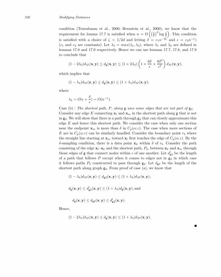
326 Modifying Distances
condition (Tenenbaum et al., 2000; Bernstein et al., 2000), we know that the
requirement for lemma 17.7 is satisfied when n = Ω((
1δ
)dlog 1
δ
). This condition
is satisfied with a choice of ζ < 1/2d and letting δ = c1n−2ζ and ǫ = c2n
−ζ)
(c1 and c2 are constants). Let λ3 = max(λ1, λ2), where λ1 and λ2 are defined in
lemmas 17.8 and 17.9 respectively. Hence we can use lemmas 17.7, 17.8, and 17.9
to conclude that
(1 − 2λ3)dM (x,y) ≤ dg(x,y) ≤ (1 + 2λ3)
(1 +
6δ
ǫ+
8δ2
ǫ2
)dM (x,y),
which implies that
(1 − λ4)dM (x,y) ≤ dg(x,y) ≤ (1 + λ4)dM (x,y),
where
λ4 = O(ǫ +δ
ǫ) = O(n−ζ).
Case (b) : The shortest path, P , along g uses some edges that are not part of g2.
Consider any edge E connecting xl and xm in the shortest path along g that is not
in g2. We will show that there is a path through g2 that can closely approximate this
edge E and hence this shortest path. We consider the case when only one section
near the endpoint xm is more than δ in Cp(α; ǫ). The case when more sections of
E are in Cp(α; ǫ) can be similarly handled. Consider the boundary point rb where
the straight line starting at xm toward xl first touches the edge of Cp(α; ǫ). By the
δ-sampling condition, there is a data point xk within δ of rb. Consider the path
consisting of the edge xl–xk and the shortest path, P2, between xk and xm through
those edges of g that connect nodes within ǫ of one another. Let d′g2 be the length
of a path that follows P except when it comes to edges not in g2 in which case
it follows paths P2 constructed to pass through g2. Let dg2 be the length of the
shortest path along graph g2. From proof of case (a), we know that
(1 − λ4)dM (x,y) ≤ dg2(x,y) ≤ (1 + λ4)dM (x,y),
dg(x,y) ≤ d′g2(x,y) ≤ (1 + λ4)dg(x,y), and
dg(x,y) ≤ dg2(x,y) ≤ d′g2(x,y).
Hence,
(1 − 2λ4)dM (x,y) ≤ dg(x,y) ≤ (1 + λ4)dM (x,y).

17.4 Semi-Supervised Learning Using Density-Based Metrics 327
17.3.2 Upper bound
In theorem 17.10, we showed that we can construct a neighborhood-based graph on
the data sample which can be used to approximately compute DBD metrics with
a rate of convergence of 1/n1/2d. This is a very slow rate of convergence, especially
when data dimension, d, is high. The natural question that follows this analysis is
whether this dependence of the rate on the data dimension is because of the curse of
dimensionality or whether it is merely because of the way the graph was constructed
and analyzed. Theorem 17.11 shows that dimension does limit how much we can
reduce the approximation error, regardless of the particular graph construction
method we use, so long as we choose to use a neighborhood-based graph. This
result is true even when data lie along a manifold, but are noisy and hence do not
lie perfectly on the manifold, i.e., the curse of dimensionality cannot be overcome
in the case of approximation error when using neighborhood-based graphs, even
when the intrinsic dimension of data is small. For this reason, this result provides
a lower bound on the approximation error of the ISOMAP algorithm (Tenenbaum
et al., 2000) as well.
Theorem 17.11 (upper bound on the computing error) The computing er-
ror, when using an ǫ-neighborhood-based graph on the data sample, cannot converge
to zero faster than 1
n1
d−1with probability ≥ δ′ for sufficiently large data sample
n ≥ N(δ′).
Proof This result is shown using an example for which the approximation error
when using the graph converges at rate 1/n1
d−1 . Consider the case when data density
is uniform over any convex set. (Note that all continuous density functions can be
approximated by a constant function in a small enough neighborhood.) In this case
the graph construction method described at the beginning of this section reduces
to an ǫ-neighborhood graph (with high probability). Consider any two points x′,x′′ in the interior of the support of the density. The shortest path between x′
and x′′ is the straight line joining them. Consider a d-dimensional cuboid which
circumscribes a cylinder of radius δ/2 around this line. If none of the points in the
data sample lie in this cuboid, the approximation error in measuring the length of
this line along the graph edges will be at least of order δ. The probability of this
happening, (1 − cδd−1)n, can be lower-bounded by a constant if δ is chosen to be
of order 1/n1
d−1 .
17.4 Semi-Supervised Learning Using Density-Based Metrics
Given a density-based distance metric, any of the nearest neighbor-based methods
(k-nearest neighbors, weighted k-nearest neighbors with various weights) can be
used for classification in a semi-supervised learning scenario. Let yi be the label of
xi and let classifier be sign(h(xi)). Let lM denote the Lipschitz constant according

328 Modifying Distances
to the manifold specified by q(p(x)). In this manifold, the lengths scale locally as
q(p(x)); hence it can be verified that for any function h on Rd
|lMh|2 = supx
1
q(p(x))| x h|2.
von Luxburg and Bousquet (2004) have shown that the 1-nearest neighbor (1NN)
classifier corresponds to a large-margin classifier. In the case of the DBD metric,a large-margin
classifier that is
equivalent to
1NN using DBD
metric
1NN is equivalent to (using the modified Lipschitz constant according to the density-
based manifold), the optimization problem
arg minh
supx
[1
q(p(x))| x h|2
]under constraints yih(xi) ≥ 1.
As p(x) increases, 1q(p(x)) also increases and hence this optimization problem
corresponds to penalizing the gradient of the classifier function h in high-density
regions and allowing h to change in the low-density regions. This agrees with
the intuition that data points in the same high-density region are likely to have
similar labels. Please see (Bousquet et al., 2004) for a discussion on regularization
appropriate for semi-supervised learning and its relationship to modifying geometry
based on the data density.
In this section, we present experimental results on data from the UCI machine
learning repository, summarized in table 17.1. The three methods we compare
are standard 1NN, DBD metric-based 1NN, and the randomized min-cut method
(Blum et al., 2004). The randomized min-cut method involves averaging over results
obtained from several min-cuts and it is suggested by Blum et al. (2004) that those
min-cuts which lead to a very unbalanced classification are to be rejected. However,
there is no clear way to choose this cutoff ratio. For the results presented here we
choose the cutoff to be slightly smaller than the “true” ratio between the classes in
the data set. For the DBD-based 1NN implementation, we chose the function q to
fall exponentially with increase in density beyond α, which in turn was chosen to
be smaller than the estimated density at all sample points.
Table 17.1 Description of data sets for the classification problem
Data set data data set class
dimension size ratio
Adult 6 1000 0.30
Abalone - 9 vs. 13 7 892 0.29
Abalone - 5 vs. 9 7 804 0.17
Digits - 1 vs. 2 256 2200 1.00
We performed experiments for labeled set size varying between 2 and 20 and
the accuracy results are shown in figure 17.3. We observed that DBD-based 1NN
performed better than or similar to the standard 1NN algorithm for all data sets

17.5 Conclusions and Future Work 329
5 10 15 20
60
65
70
% A
ccu
racy
# Labeled points
Adult
5 10 15 20
50
55
60
65
70
% A
ccu
racy
# Labeled points
Abalone - 9 vs 13
5 10 15 20
60
70
80
90
% A
ccu
racy
# Labeled points
Abalone - 5 vs 9
5 10 15 20
70
75
80
85
90
% A
ccu
racy
# Labeled points
Digits - 1 vs 2
Figure 17.3 Classification results comparing 1NN (.), DBD-based 1NN (x) and ran-domized min-cut (o) algorithms.
with small dimension. We conjecture that the reason DBD-based 1NN performed
worse than 1NN for the digits example is because of difficulty in density estimation
in very high dimensions. The DBD-based 1NN algorithm performed better than
the other two when the number of labeled examples was very small, except in the
case of the digits example. One interesting result was that of the two abalone data
examples, in which the randomized min-cut algorithm performed much better than
both NN algorithms in one case and much worse in the other.
17.5 Conclusions and Future Work
We have shown that density-based distance metrics which satisfy certain properties
can be estimated consistently using an estimator obtained by plugging in the kernel
density estimate of the data distribution. In terms of s, a smoothness parameter
that corresponds to how many times data density is known to be differentiable
and d, the data dimension, we have shown that the rate of convergence of such an
estimator is s2s+d . We have also shown that no estimator can converge at a rate

330 Modifying Distances
faster than 12 .
This contains both good and bad news. The knowledge that we have consistent
estimation is useful when applying the method to voluminous data (for example,
webpages). However, we expect d to be high for many machine learning applications
and we might not be able to assume that the smoothness parameter, s, is very high.
Hence, when using the plug-in estimator, the convergence rate can be very slow for
high-dimensional data.
We have shown a graph construction method that can be used for consistent com-
putation of DBD metrics and shown that with high probability, the approximation
error when using this graph goes to zero faster than 1/n1/2d with high probability.
We have also shown that the shortest distance along a nearest neighborhood-based
graph on the data cannot converge to true distance faster than 1/n1/(d−1) with high
probability. We presented semi-supervised classification results that demonstrate
that using DBD metrics can sometimes improve performance over using simple
Euclidean distance, when data density can be estimated with reasonable reliability.
While we have been able to give a theoretical understanding of DBD metrics, fur-
ther experimental investigation of their use for semi-supervised learning in needed to
make them a practically viable choice. While several papers have considered DBD
metrics, the only papers that present experimental results with real world data
use the 1NN algorithm (Lebanon, 2003; Sajama and Orlitsky, 2005). Experiments
using these metrics with other classification algorithms, using parametric density
estimation in place of the kernel density estimator, and studying alternative graph
construction and weighting methods for more accurate and efficient computation
will be of practical value.
Acknowledgements
We thank Sanjoy Dasgupta and Thomas John for several helpful discussions.
Thanks also to anonymous reviewers for several comments used in revising and
improving this paper. In particular, we thank an anonymous reviewer for pointing
out an error in the analysis of the estimation error rate in an earlier version.

V Semi-Supervised Learning in Practice


18 Large-Scale Algorithms
Olivier Delalleau [email protected]
Yoshua Bengio [email protected]
Nicolas Le Roux [email protected]
In chapter 11, it is shown how a number of graph-based semi-supervised learning
algorithms can be seen as the minimization of a specific cost function, leading to a
linear system with n equations and unknowns (with n the total number of labeled
and unlabeled examples). Solving such a linear system will in general require on the
order of O(kn2) time and O(kn) memory (for a sparse graph where each data point
has k neighbors), which can be prohibitive on large data sets (especially if k = n,
i.e., the graph is dense). We present in this chapter a subset selection method that
can be used to reduce the original system to one of size m ≪ n. The idea is to solve
for the labels of a subset S ⊂ X of only m points, while still retaining information
from the rest of the data by approximating their label with a linear combination
of the labels in S (using the induction formula presented in chapter 11). This leads
to an algorithm whose computational requirements scale as O(m2n) and memory
requirements as O(m2), thus allowing one to take advantage of significantly bigger
unlabeled data sets than with the original algorithms.
18.1 Introduction
The graph-based semi-supervised algorithms presented in chapter 11 do not scale
well to very large data sets. In this chapter, we propose an approximation method
that significantly reduces the computational and memory requirements of such
algorithms. Notations will be the same as in chapter 11, i.e.:
Y = (Yl, Yu) is the set of “original” labels on labeled and unlabeled points (here,
Yu is filled with 0),
Y = (Yl, Yu) is the set of estimated labels on labeled and unlabeled points,
y is the function to learn, which assigns a label to each point of the input space,

334 Large-Scale Algorithms
y(xi) = yi is the value of the function y on training points (labeled and unlabeled).
In chapter 11, we defined a quadratic cost (Eq. 11.11):
C(Y ) = ‖Yl − Yl‖2 + μY ⊤LY + μǫ‖Y ‖2. (18.1)
Minimizing this cost gives rise to the following linear system in Y with regularization
hyperparameters μ and ǫ:
(S + μL + μǫI) Y = SY, (18.2)
where S is the (n × n) diagonal matrix defined by Sii = δi≤l, and L = D − W is
the un-normalized graph Laplacian. This linear system can be solved to obtain the
value of yi on the training points xi. We can extend the formula to obtain the value
of y on every point x in the input space as shown in section 11.4:
y =
∑j WX(x, xj)yj∑
j WX(x, xj) + ǫ. (18.3)
where WX is the symmetric data-dependent edge weighting function (e.g., a
Gaussian kernel) such that Wij = WX(xi, xj). However, in case of very large
training sets, solving the linear system (18.2) may be computationally prohibitive,
even using iterative techniques such as those described in section 11.2. In this
chapter we consider how to approximate the cost using only a subset of the
examples. Even though this will not yield an exact solution to the original problem,
it will make the computation time much more reasonable.
18.2 Cost Approximations
18.2.1 Estimating the Cost from a Subset
A simple way to reduce the O(kn2) computational requirement and O(kn) memory
requirement for training the non-parametric semi-supervised algorithms of chap-
ter 11 is to force the solutions to be expressed in terms of a subset of the examples.
This idea has already been exploited successfully in a different form for other ker-reduced
parametrization
of solution
nel algorithms, e.g., for Gaussian processes (Williams and Seeger, 2001) or spectral
embedding algorithms (Ouimet and Bengio, 2005).
Here we will take advantage of the induction formula (Eq. 18.3) to simplify the
linear system to m ≪ n equations and variables, where m is the size of a subset
of examples that will form a basis for expressing all the other function values. Let
S ⊂ 1, . . . , n be a subset, with |S| = m and S ⊃ 1, . . . , l (i.e., we take all
labeled examples in the subset). Define R = 1, . . . , n\S (the rest of the data).
In the following, vector and matrices will be split into their S and R parts, e.g.

18.2 Cost Approximations 335
Y = (YS , YR) and
L =
(LSS LSR
LRS LRR
).
The idea is to force yi ∈ YR to be expressed as a linear combination of the yj ∈ YS
following (18.3):
∀i ∈ R, yi =
∑j∈S Wij yj∑
j∈S Wij + ǫ(18.4)
or in matrix notation
YR = WRSYS (18.5)
with WRS the matrix of size ((n − m) × m) with entries Wij/(ǫ +∑
k∈S Wik),
for i ∈ R and j ∈ S. We will then split the cost (18.1) in terms that involve only
the subset S or the rest R, or both of them. To do so, we must first split the
diagonal matrix D (whose elements are row sums of W) into D = DS + DR, with
DS and DR the (n × n) diagonal matrices whose elements are sums over S and R
respectively, i.e.,
DSii =
∑
j∈S
Wij
DRii =
∑
j∈R
Wij .
The unnormalized Laplacian L = D− W can then be written
L =
(DS
SS + DRSS − WSS −WSR
−WRS DSRR + DR
RR − WRR
). (18.6)
Using (18.6), the cost (18.1) can now be expanded as follows:
C(Y ) = μY ⊤LY + μǫ‖Y ‖2 + ‖Yl − Yl‖2
= μY ⊤S
(DS
SS − WSS
)YS + μǫ‖YS‖2
︸ ︷︷ ︸CSS
+ μY ⊤R
(DR
RR − WRR
)YR + μǫ‖YR‖2
︸ ︷︷ ︸CRR
+ μ(Y ⊤
S DRSS YS + Y ⊤
R DSRRYR − Y ⊤
R WRSYS − Y ⊤S WSRYR
)
︸ ︷︷ ︸CRS
+ ‖Yl − Yl‖2
︸ ︷︷ ︸CL
.

336 Large-Scale Algorithms
18.2.2 Resolution
Using the approximation YR = WRSYS (18.5), the gradient of the different parts
of the above cost with respect to YS is then
∂CSS
∂YS
=[2μ
(DS
SS − WSS + ǫI)]
YS
∂CRR
∂YS
=[2μW
⊤RS
(DR
RR − WRR + ǫI)WRS
]YS
∂CRS
∂YS
=[2μ
(DR
SS + W⊤RSDS
RRWRS − W⊤RSWRS − WSRWRS
)]YS
=[2μ
(DR
SS − WSRWRS
)]YS (18.7)
∂CL
∂YS
= 2SSS(YS − Y ),
where to obtain (18.7) we have used the equality DSRRWRS = WRS , which follows
from the definition of WRS .
Recall the original linear system in Y was (S + μL + μǫI) Y = SY (18.2). Here
it is replaced by a new system in YS , written AYS = SSSYS with
A = μ(DS
SS − WSS + ǫI + DRSS − WSRWRS
)
+ μW⊤RS
(DR
RR − WRR + ǫI)WRS
+ SSS .
Since the system’s size has been reduced from n to |S| = m, it can be solved much
faster, even if A is not guaranteed1 to be sparse anymore (we assume m ≪ n).
Unfortunately, in order to obtain the matrix A, we need to compute DRRR, which
costs O(n2) in time, as well as products of matrices that cost O(mn2) if W is not
sparse. A simple way to get rid of the quadratic complexity in n is to ignore CRRsimplified cost
function in the total cost. If we remember that CRR can be written
CRR = μ
⎛
⎝1
2
∑
i,j∈R
Wij(yi − yj)2 + ǫ‖YR‖2
⎞
⎠ ,
this corresponds to ignoring the smoothness assumption between points in R, as
well as the regularization term on R. Even if it may look like a bad idea, it turns
out it usually preserves (and even improves) the performance of the semi-supervised
classifier, for various reasons:
Assuming the subset S is chosen to correctly “fill” the space, smoothness between
points in S and points in R (encouraged by the part CRS of the cost) also enforces
smoothness between points in R only.
1. In practice, if W is sparse, A is also likely to be sparse, even if additional assumptionson W are needed if one wants to prove it.

18.3 Subset Selection 337
When reducing to a subset, the loss in capacity (we can choose m values instead
of n when working with the full set) suggests we should weaken regularization,
and the smoothness constraints are a form of regularization; thus dropping some of
them is a way to achieve this goal.
For some points i ∈ R, the approximation (18.4)
yi =
∑j∈S Wij yj∑
j∈S Wij + ǫ
may be poor (e.g. for a point far from all points in S, i.e.∑
j∈S Wij very small);
thus smoothness constraints between points in R could be noisy and detrimental
to the optimization process (this is not a big issue when considering smoothness
between a point xi in R and a point xj in S as the smoothness penalty is weighted
by Wij , which will be small if xi is far from all points in S).
Given the above considerations, ignoring the part CRR leads to the new system
(SSS + μ
(DSS − WSS − WSRWRS + ǫI
))YS = SSSYS
which in general can be solved in O(m3) time (less if the system matrix is sparse).
18.3 Subset Selection
18.3.1 Random Selection
In general, training using only a subset of m ≪ n samples will not perform as well
as using the whole data set. Carefully choosing the subset S can help in limiting
this loss in performance. Even if random selection is certainly the easiest way to
choose the points in S, it has two main drawbacks:
It may not pick points in some regions of the space, resulting in the approximation
(18.4) being very poor in these regions.
It may pick uninteresting points: the region near the decision surface is the one
where we are more likely to make mistakes by assigning the wrong label. Therefore,
we would like to have as many points as possible in S being in that region, while
we do not need points which are far away from that surface.
As a result, it is worthwhile considering more elaborate subset selection schemes,
such as the one presented in the next section.
18.3.2 Smart Data Sampling
There could be many ways of choosing which points to take in the subset. The
algorithm described below is one solution, based on the previous considerations
about the random selection weaknesses. The first step of the algorithm will be

338 Large-Scale Algorithms
to select points somewhat uniformly in order to get a first estimate of the decision
surface, while the second step will consist in the choice of points near that estimated
surface.
18.3.2.1 First Step
Equation 18.4,
yi =
∑j∈S Wij yj∑
j∈S Wij + ǫ,
suggests that the value of yi is well approximated when there is a point in S near
xi (two points xi and xj are nearby if Wij is high). The idea will therefore be to
cover the manifold where the data lie as well as possible, that is to say ensure thatcovering the
manifold every point in R is near a point (or a set of points) in S. There is another issue we
should be taking care of: as we discard the part CRR of the cost, we must now be
careful not to modify the structure of the manifold. If there are some parts of the
manifold without any point of S, then the smoothness of y will not be enforced at
such parts (and the labels will be poorly estimated).
This suggests starting with S = 1, . . . , l and R = l + 1, . . . , n, then adding
samples xi by iteratively choosing the point farthest from the current subset, i.e.
the one that minimizes∑
j∈S Wij . The idea behind this method is that it is useless
to have two points near each other in S, as this will not give extra information
while increasing the cost. However, one can note that this method may tend to
select outliers, which are far from all other points (and especially those from S).
A way to avoid this is to consider the quantity∑
j∈R\i Wij for a given xi. If xiavoiding outliers
is such an outlier, this quantity will be very low (as all Wij are small). Thus, if it
is smaller than a given threshold δ, we do not take xi in the subset. The cost of
this additional check is of O((m + o)n) where o is the number of outliers: assuming
there are only a few of them (less than m), it scales as O(mn).
18.3.2.2 Second Step
Once this first subset is selected, it can be refined by training the algorithm
presented in section 11.3.2 on the subset S, in order to get an approximation of the
yi for i ∈ S, and by using the induction formula 18.4 to get an approximation of the
yj for j ∈ R. Samples in S which are far away from the estimated decision surfacediscarding
uninformative
samples
can then be discarded, as they will be correctly classified no matter whether they
belong to S or not, and they are unlikely to give any information on the shape of
the decision surface. These discarded samples are then replaced by other samples
that are near the decision surface, in order to be able to estimate it more accurately.
The distance from a point xi to the decision surface is estimated by the confidence
we have in its estimated label yi. In the binary classification case considered here
(with targets −1 and 1), this confidence is given by |yi|, while in a multiclass setting
it would be the absolute value of the difference between the predicted scores of the

18.3 Subset Selection 339
two highest-scoring classes. One should be careful when removing samples, though:
we must make sure we do not leave “empty” regions. This can be done by ensuring
that∑
j∈S Wij stays above some threshold for all i ∈ R after a point has been
removed.
Overall, the cost of this selection phase is on the order of O(mn + m3). It is
summarized in algorithm 18.1.
Algorithm 18.1 Subset selection
Choose a small threshold δ (e.g. δ ← 10−10)
Choose a small regularization parameter ǫ (e.g. ǫ ← 10−11)
(1) Greedy selection
S ← 1, . . . , l The subset we are going to build contains the labeled pointsR ← l + 1, . . . , n The rest of the unlabeled pointswhile |S| < m do
Find i ∈ R s.t.∑
j∈R\i Wij ≥ δ and∑
j∈S Wij is minimum
S ← S ∪ iR ← R \ i
end while
(2) Decision surface improvement
Compute an approximate of yi with i ∈ S by applying the standard semi-
supervised minimization of section 11.3.2 with the data set S
Compute an approximate of yj with j ∈ R by (18.4)
SH ← the points in S with highest confidence (see section 18.3.2.2)
RL ← the points in R with lowest confidence
for all i ∈ SH do
if minj∈R
∑k∈S\i Wjk ≥ δ then
i can be safely removed from S without leaving empty regionsk∗ ← argmink∈RL
∑j∈S Wjk Find point with low confidence farthest from
SReplace i by k∗ in S (and k∗ by i in R)
end if
end for
18.3.3 Computational Issues
We are now in position to present the overall computational requirements for the
different algorithms proposed in this chapter. As before, the subset size m is taken
to be much smaller than the total number of points n, and the weight matrix
W may either be dense or sparse (with k non-zero entries in each row or column).
Table 18.1 summarizes time and memory requirements for the following algorithms:

340 Large-Scale Algorithms
Table 18.1 Comparative computational requirements of NoSub, RandSub, and Smart-Sub (n = number of labeled and unlabeled training data, m = subset size with m ≪ n, k= number of neighbors for each point in W when W is sparse)
Time Memory
NoSub (sparse W) O(kn2) O(kn)
NoSub (dense W) O(n3) O(n2)
RandSub O(m2n) O(m2)
SmartSub O(m2n) O(m2)
NoSub: the original transductive algorithm (using the whole data set) that consists
in solving the system (18.2), as presented in chapter 11 (algorithm 11.2),
RandSub: the approximation algorithm discussed in section 18.2.2, with the subset
S being randomly chosen (section 18.3.1),
SmartSub: the same approximation algorithm as RandSub, but with S being
chosen as in section 18.3.2.
The table shows that the approximation method described in this chapter is
particularly useful when W is dense or n is very large. This is confirmed by
empirical experimentation in figure 18.1, which compares the training times (on the
benchmark data set SecStr described in chapter 21 of this book) of NoSub with a
dense kernel, NoSub with a sparse kernel, and SmartSub with a dense kernel. With
a dense kernel, NoSub becomes quickly impractical because of the need to store
(and solve) a linear system of size n = l + u, with l = 100 and u ∈ [2000, 50, 000].
With a sparse kernel (and the iterative version presented in algorithm 11.2) it scales
much better, but still exhibits a quadratic dependency in n. On the other hand,
SmartSub can handle much more unlabeled data as its training time scales only
linearly in n. We have not presented a sparse version of SmartSub since our current
code cannot take advantage of a sparse weighting function. However, this could be
useful to obtain further improvement, especially in terms of memory usage (working
with full m × m matrices can become problematic when m ≥ 10, 000).
18.4 Discussion
This chapter follows up on chapter 11 to allow large-scale applications of semi-
supervised learning algorithms presented previously. The idea is to express the cost
to be minimized as a function of only a subset of the unknown labels, in order to
reduce the number of free variables: this can be obtained thanks to the induction
formula introduced in chapter 11. The form of this formula suggests it is only
accurate when the points in the subset cover the whole manifold on which the data
lie. This explains why choosing the subset randomly can lead to poor results, while

18.4 Discussion 341
0 10,000 20,000 30,000 40,000 50,0000
500
1000
1500
NoSub (dense W)
NoSub (sparse W)
SmartSub (dense W)
Figure 18.1 Training time (in seconds) w.r.t. the amount of unlabeled samples onbenchmark data set SecStr (cf. chapter 21). WX is a Gaussian kernel (combined withan approximate 100-nearest-neighbor kernel in the sparse case). There are l = 100 labeledsamples, and SmartSub selects m = 500 unlabeled samples in the subset approximationscheme. Note how the dependence of SmartSub in the total number of unlabeled samplesu ∈ [2000, 50, 000] is only linear. NoSub with dense W fails for u ≥ 10, 000 because ofmemory shortage. Experiments were performed on a 3.2GHz P4 CPU with 2Gb of RAM.
it is possible to design a simple heuristic algorithm (such as algorithm 18.1) giving
much better classification performance. Better selection algorithms (e.g., explicitly
optimizing the cost we are interested in) are the subject of future research.
One must note that the idea of expressing the cost from a subset of the data is
not equivalent to training a standard algorithm on the subset only, before extending
to the rest of the data with the induction formula. Here, the rest of the data are
explicitly used in the part of the cost enforcing the smoothness between points in
the subset and points in the rest (part CRS of the cost), which helps to obtain a
smoother labeling function, usually giving better generalization.


19 Semi-Supervised Protein Classification
Using Cluster Kernels
Jason Weston [email protected]
Christina Leslie [email protected]
Eugene Ie [email protected]
William Stafford Noble [email protected]
In this chapter we describe an experimental study of large-scale semi-supervised
learning for the problem of protein classification. The protein classification prob-
lem, a central problem in computational biology, is to predict the structural class
of a protein given its amino acid sequence. Such a classification helps biologists to
understand the function of a protein. Building an accurate protein classification
system, as in many tasks, depends critically upon choosing a good representation
of the input sequences of amino acids. Early work using string kernels with support
vector machines (SVMs) for protein classification achieved state-of-the-art classifi-
cation performance. However, such representations are based only on labeled data—
examples with known three-dimensional (3D) structures, organized into structural
classes—while in practice, unlabeled data are far more plentiful.
This chapter compares different approaches that extend these earlier results to
take advantage of unlabeled data. In particular, special cases of cluster kernels
are described that are scalable to hundreds of thousands of unlabeled points and
provide state-of-the-art performance.
19.1 Introduction
The 3D structure that a protein assumes after folding largely determines its function
in the cell. However, it is far easier to determine experimentally the primary
sequence (the string of amino acids) that make up a protein than it is to discover
its 3D structure. Through evolution, structure is more conserved than sequence,protein remote
homology
detection
so that detecting even very subtle sequence similarities, or remote homology, is

344 Semi-Supervised Protein Classification Using Cluster Kernels
important for predicting structure, which can help infer function. Computational
techniques have proven very successful at aiding biologists in this task.
The major methods for homology detection can be split into three basic groups:
pairwise sequence comparison algorithms (Altschul et al., 1990; Smith and Wa-
terman, 1981), generative models for protein families (Krogh et al., 1994; Park
et al., 1998), and discriminative classifiers (Jaakkola et al., 2000; Leslie et al., 2003;
Liao and Noble, 2002). Popular sequence comparison methods such as BLAST and
Smith-Waterman are based on alignment scores. Generative models such as profile
hidden Markov models (HMMs) model positive examples of a protein family, but
these models can be trained iteratively using both positively labeled and unlabeled
examples by pulling in close homologs and adding them to the positive set. A com-
promise between these methods is PSI-BLAST (Altschul et al., 1997), which uses
BLAST to iteratively build a probabilistic profile of a query sequence and obtain a
more sensitive sequence comparison score.
Finally, classifiers such as support vector machines (SVMs) use both positive
and negative examples and provide state-of-the-art performance when used with
appropriate distance metrics (i.e., appropriate kernels) (Jaakkola et al., 2000; Leslie
et al., 2003; Liao and Noble, 2002; Saigo et al., 2004). To be more specific, to solve
this task as a classification problem, the input is the string of amino acids: the
string is typically hundreds of “characters” in length, and the characters themselves
have an alphabet of size 20. Posed as a binary classification problem, a classifier
can answer the question: “Does the given protein (amino acid sequence) belong
to structural class X or not?” and should be trained with positive and negative
examples of this class.
Building an accurate system, as in most machine learning tasks, depends critically
upon choosing a good representation of the input sequences of amino acids. The first
hurdle is that the inputs are not vectors of fixed dimension, and so to use standard
methods like SVMs one must define a similarity on sequences. This is possible by
using string kernels, whereby one embeds the strings into a vector space and then
performs inner products in this space. This issue is discussed in section 19.2. A
study of the performance of these methods compared to more classical techniques
is also detailed there.
In practice, however, relatively little labeled data are available—approximately
30,000 proteins with known 3D structure, some belonging to families and superfam-
ilies with only a handful of labeled members—whereas there are close to one million
sequenced proteins, providing abundant unlabeled data. The basic method in the
literature (Jaakkola et al., 2000; Leslie et al., 2003) to take advantage of this extra
data is to use an auxiliary method (such as PSI-BLAST) in order to add predicted
homologs of the positive training examples to the training set before training the
classifier. New semi-supervised learning techniques should be able to make bettersemi-supervised
learning use of these unlabeled data.
Some of the recent work in semi-supervised learning has focused on changing the
representation given to a classifier by taking into account the structure described by
the unlabeled data (Chapelle et al., 2003; Szummer and Jaakkola, 2002b). These

19.2 Representations and Kernels for Protein Sequences 345
efforts can be viewed as cases of cluster kernels, which learn similarity metrics
based on the cluster assumption: when two points are in the same “cluster” (or are
connected by a path of high density) in the original metric they should have a small
distance to each other in the new metric. This review describes an experimentalcluster kernels
comparison of cluster kernels and some other competing methods on the protein
classification problem. In particular, two simple and scalable cluster kernel methods
will be described that were developed explicitly for this problem. The neighborhood
kernel (Weston et al., 2003a) uses averaging over a neighborhood of sequences
defined by a local sequence similarity measure, and the bagged kernel (Weston et al.,
2003a) uses bagged clustering of the full sequence data set to modify the base kernel.
Finally, we compare these two methods to a problem-specific solution, the profile
kernel of Kuang et al. (2004). In this kernel, each sequence is represented by a profile
estimated from a large unlabeled database (using PSI-BLAST, for example); the
profile kernel uses a substring-based feature map, but is defined on sequence profiles
rather than the sequences themselves.
In both the semi-supervised and transductive settings, these last three techniques
all provide greatly improved classification performance when used with mismatch
string kernels, and the techniques achieve equal or superior results to all previ-
ously presented cluster kernel methods that we tried. Moreover, they are far more
computationally efficient than these competing methods. The profile kernel pro-
vides perhaps the best scalability, whereas the neighborhood and bagged kernels
provide similar performance and good scaling ability, while providing more general
applicability.
The chapter is organized as follows. We begin with an overview of sequence
representations for supervised classifiers in section 19.2, followed in section 19.3 by
a review of existing cluster kernel methods for incorporating unlabeled data into
the kernel representation. In sections 19.3.2, 19.3.3, and 19.3.4, we describe the
profile, neighborhood, and bagged mismatch kernels. Finally, detailed experiments
comparing these techniques are given in section 19.4.
19.2 Representations and Kernels for Protein Sequences
Proteins can be represented as variable-length sequences, typically several hundred
characters long, from the alphabet of 20 amino acids. In order to use learning
algorithms that require vector inputs, we must first find a suitable feature vector
representation, mapping sequence x into a vector space by x → Φ(x). Kernel
methods such as SVMs only need to compute inner products, called kernels,
k(x, y) = 〈Φ(x), Φ(y)〉, for training and testing. We thus can accomplish the above
mapping using a kernel for sequence data.
Biologically motivated sequence comparison scores, like Smith-Waterman or
BLAST, provide an appealing representation of sequence data. The Smith-
Waterman (SW) algorithm (Smith and Waterman, 1981) uses dynamic program-
ming to compute the optimal local gapped alignment score between two sequences,

346 Semi-Supervised Protein Classification Using Cluster Kernels
while BLAST (Altschul et al., 1990) approximates SW by computing a heuristic
alignment score. Both methods return empirically estimated E-values1 indicating
the confidence of the score. These alignment-based scores do not define a positive
definite kernel; however, one can use a feature representation based on the empirical
kernel mapempirical kernel
mapΦ(x) = (d(x1, x), . . . , d(xl, x)),
where d(x, y) is the pairwise score (or E-value) between x and y, and xi for
i = 1, . . . , l are the training sequences. Using SW E-values in this fashion —
the SVM-pairwise method (Liao and Noble, 2002)— gives strong classification
performance. Note, however, that SVM-pairwise is slow, both because computing
each SW score is O(|x|2) and because computing each empirically mapped kernel
value is O(l).
Another appealing idea is to derive the feature representation from a generative
model for a protein family. In the Fisher kernel method (Jaakkola et al., 2000),
one first builds a profile HMM for the positive training sequences, defining a
log-likelihood function logP (x|θ) for any protein sequence x. Then the gradientFisher kernel
vector ∇θ log P (x|θ)|θ=θ0 ,where θ0 is the maximum-likelihood estimate for model
parameters, defines an explicit vector of features, called Fisher scores, for x. This
representation gives excellent classification results, but the Fisher scores must be
computed by an O(|x|2) forward-backward algorithm, making the kernel tractable
but slow.
It is possible to construct useful kernels directly without explicitly depending on
generative models by using string kernels. For example, the mismatch kernel (Leslie
et al., 2003) is defined by a histogram-like feature map that uses mismatches to
capture inexact string matching. The feature space is indexed by all possible p-p-gram string
kernels length subsequences α = a1, a2, . . . , ap, where each ai is a character in the alphabet
A of amino acids. The feature map is defined on p-gram α by Φ(α) = (φβ(α))Ap ,
where φβ(α) = 1 if α is within m mismatches of β, and 0 otherwise. The feature
map is extended additively to longer sequences: Φ(x) =∑
p-gramsα∈x Φ(α). The
mismatch kernel can be computed efficiently using a trie data structure: the
complexity of calculating k(x, y) is O(ck(|x| + |y|)), where ck = pm+1|A|m. For
typical kernel parameters p = 5 and m = 1 (Leslie et al., 2003), the mismatch
kernel is fast, scalable, and yields impressive performance.string kernels
Other direct string kernel methods include pair HMM and convolution kernels
(Watkins, 1999; Haussler, 1999; Lodhi et al., 2002), which are quite general but also
have complexity O(|x||y|); more recent and related string alignment kernels (Saigo
et al., 2004), also with complexity O(|x||y|); and exact-matching string kernels built
with suffix trees and suffix links, with complexity O(|x| + |y|) (Vishwanathan and
1. The E-value is the expected number of times that an alignment score as good or betterthan the observed score is expected to appear by chance in a random sequence databaseof the given size.

19.2 Representations and Kernels for Protein Sequences 347
0 0.2 0.4 0.6 0.8 10
10
20
30
40
50
60
ROC
Num
ber
of fa
mili
es w
ith g
iven p
erf
orm
ance
SVM−SWSVM−MISMATCHSVM−BLASTSVM−fisherSAMPSI−BLASTknn−SW
Figure 19.1 Comparison of protein representations and classifiers without use of unla-beled data. The graph plots the total number of families for which a given method exceeds aROC score threshold. The SVM-based methods use the following kernels: Smith-Watermanempirical kernel map (SW), mismatch kernel with p = 5 and m = 1 (mismatch), BLASTempirical kernel map (BLAST), and a Fisher kernel built from a profile HMM (Fisher).The three non-SVM methods include a hidden Markov model (SAM), the PSI-BLASTalgorithm, and the kernel k-nearest neighbor algorithm (k=3) using a Smith-Watermanempirical kernel map.
Smola, 2002). Inexact string matching models similar to the mismatch kernel but
with complexity O(ck(|x| + |y|)), with ck independent of alphabet size, have also
been presented (Leslie and Kuang, 2003). The motif kernel (Ben-Hur and Brutlag,
2003) uses features that are built from a fixed database of motifs; computing these
features is linear in the length of the sequence. Finally, almost all these kernels
can be constructed using the rational kernel framework of Cortes et al. (2002). We
concentrate on the mismatch kernel representation for the current work.
In figure 19.1, we summarize the results from Liao and Noble (2002) and Leslie
et al. (2003) by comparing SVM performance with these representations and other
homology detection methods on a problem that does not include the use of unlabeled
data. These and subsequent experiments are based upon the structural classification
of proteins (SCOP) (Murzin et al., 1995). This is a widely used database of
protein structures, in which proteins are organized hierarchically into classes, folds,
superfamilies, and families. SCOP contains only proteins for which the 3D structure
is available; hence, related proteins can be placed into a single superfamily even
when their amino acid sequences have diverged evolutionarily. The SCOP database
has been used in a large number of published studies of protein homology detection

348 Semi-Supervised Protein Classification Using Cluster Kernels
and fold classification algorithms. Here, we use a benchmark data set of Liao and
Noble (2002), which consists of 54 two-class remote homology detection problems.
The positive test set is a target protein family to be detected, and the positive
training set contains sequences that are only remotely related to the target. The
negative training and test sets are proteins from two disjoint sets of folds, and
contain no proteins from the target fold. All methods are evaluated by using receiver
operating characteristic (ROC) scores. More details concerning the experimental
setup can be found at http://www1.cs.columbia.edu/compbio/svm-pairwise.
The results indicate that, without unlabeled data, SVM methods using a number
of representations perform very strongly. They are superior to both HMMs (SAM-
T98 (Park et al., 1998)) and pairwise scoring functions like PSI-BLAST. We believe
that the SVM Fisher kernel computed here performs poorly because the underlying
HMMs lack sufficient training data. (For a method comparison in the more standard
setting, where domain homologs from an unlabeled database are added to the
training set, see Leslie et al. (2003); there, SVM-Fisher is competitive with the
mismatch kernel.) Note, however, that the performance of k-nearest neighbors (k-
NN) with a good representation (the SW representation) performs poorly, so choice
of classifier is also important.
It seems clear that string kernel methods with SVMs are a powerful approach,
but in a real-world setting, classifiers have access to unlabeled data. We now discuss
how to incorporate such data into the representation given to SVMs via the use of
cluster kernels.
19.3 Semi-Supervised Kernels for Protein Sequences
In semi-supervised learning, one tries to improve a classifier trained on labeled data
by exploiting a relatively large set of unlabeled data. The most common assumptioncluster
assumption one makes in this setting is called the “cluster assumption,” namely that the class
does not change in regions of high density. Equivalently, one assumes that the true
decision boundary lies in regions of low density.
19.3.1 Existing Cluster Kernels
We will focus on classifiers that re-represent the given data to reflect structure
revealed by unlabeled data. The main idea is to change the distance metric so that
the relative distance between two points is smaller if the points are in the same
cluster. If one is using kernels, rather than explicit feature vectors, one can modify
the kernel representation by constructing a cluster kernel.
Previous work of Chapelle et al. (2003) presented a general framework for
producing cluster kernels by modifying the eigenspectrum of the kernel matrix.
Two of the main methods presented are the random walk kernel and the spectralrandom walk and
spectral
clustering kernels
clustering kernel, which we will briefly summarize below. See chapter 15 for more
details on these and other spectral cluster kernels.

19.3 Semi-Supervised Kernels for Protein Sequences 349
The random walk kernel is a normalized and symmetrized version of a transition
matrix corresponding to a t-step random walk. As described in Szummer and
Jaakkola (2002b), one can define a random walk representation by viewing a radial
basis function (RBF) kernel as a transition matrix of a random walk on a graph
with vertices xi. One then uses the eigendecomposition of the normalized transition
matrix to compute the t-step random walk kernel. The spectral clustering kernel is
a simple use of the representation derived from spectral clustering (Ng et al., 2002)
using the first k eigenvectors of a normalized affinity matrix.
A serious problem with these methods is that one must diagonalize a matrix of
size n, where n is the number of labeled and unlabeled data, giving a complexity
O(n3). Other methods of implementing the cluster assumption such as transductive
SVMs (Joachims, 1999), described in chapter 6, also suffer from computational
efficiency issues. A second drawback is that these kernels are better suited to
a transductive setting (where one is given both the unlabeled and test points in
advance) rather than a semi-supervising setting. In sections 19.3.2 and 19.3.3, we
will describe two simple methods to implement the cluster assumption that do not
suffer from these issues.
19.3.2 The Neighborhood Kernel
In this section and the next, we introduce two fast and general cluster kernels that
leverage unlabeled data to improve a base kernel representation. Unlike other clusterfast cluster
kernels kernel approaches, these kernels make use of two complementary (dis)similarity
measures: a base kernel representation which implicitly makes use of features useful
for discrimination between classes, and a distance measure that describes how close
examples are to each other. In our application to protein classification, we use the
mismatch string kernel as the base kernel and standard sequence comparison metrics
(such as BLAST or PSI-BLAST E-values) as the distance measure. We note that
string kernels have proved to be powerful representations for SVM classification
(Leslie et al., 2003) but do not give sensitive pairwise similarity scores like the
BLAST family methods; thus the two sequence similarity measures play distinct
roles in the kernel definition.
For the neighborhood kernel, we use a standard sequence dissimilarity measure
like BLAST or PSI-BLAST to define a neighborhood for each input sequence. Theneighborhood
kernel neighborhood Nbd(x) of sequence x is the set of sequences x′ with similarity score
to x below a fixed E-value threshold, together with x itself. Now given a fixed
original feature representation, we represent x by the average of the feature vectors
for members of its neighborhood: Φnbd(x) =1
|Nbd(x)|∑
x′∈Nbd(x) Φorig(x′). The
neighborhood kernel is then defined by
knbd(x, y) =
∑x′∈Nbd(x),y′∈Nbd(y) korig(x
′, y′)
|Nbd(x)||Nbd(y)| .
We will see in the experimental results that this simple neighborhood-averaging

350 Semi-Supervised Protein Classification Using Cluster Kernels
Figure 19.2 Neighborhood averaging for a toy data set. Feature representationsfor a toy data set before (left) and after (right) the neighborhood averaging operation.The shaded region is the union of the convex hulls of the neighborhood point sets for theoriginal data.
technique, used in a semi-supervised setting with the mismatch kernel, dramatically
improves classification performance.
In general, computing each neighborhood kernel value is quadratic in neighbor-
hood size, as is clear from the kernel expression given above. However, in the special
case where we use the mismatch kernel as base kernel, we can modify the mismatch
kernel algorithm by presenting each neighborhood set as a concatentation of the
neighbor sequences (keeping track of where the ends of sequences are located); us-
ing a trie data structure, the kernel computation is linear in sequence length, giving
a complexity of O(pm+1|A|m(∑
x′ +∑
y′)) (that is, linear in neighborhood size)
to compute knbd(x, y), where |A| is the size of the alphabet of amino acids (Leslie
et al., 2003).
To see how the neighborhood approach fits with the cluster assumption, consider
a set of points in feature space that form a “cluster” or dense region of the data
set, and consider the region R formed by the union of the convex hulls of the
neighborhood point sets. If the dissimilarity measure is a true distance, then the
neighborhood averaged vector Φnbd(x) stays inside the convex hull of the vectors in
its neighborhood, and all the neighborhood vectors stay within region R. In general,
the cluster contracts inside R under the averaging operation. Thus, under the new
representation, different clusters can become better separated from each other.
Figure 19.2 gives an illustration of this phenomenon for a toy data set, showing
the contraction of clusters within region R after neighborhood averaging.
19.3.3 The Bagged Cluster Kernel
A number of existing clustering techniques are much more efficient than the methods
mentioned in section 19.3. For example, the classical k-means algorithm is O(rknd),
where n is the number of data points, d is their dimensionality, and r is the number

19.3 Semi-Supervised Kernels for Protein Sequences 351
of iterations required. Empirically, this running time grows sublinearly with k, n,
and d. Therefore, in practice, it is computationally efficient to run k-means multiple
times, which can be useful because it can converge to local minima. We therefore
consider the following method:bagged kernel
1. Run k-means N times, giving j = 1, . . . , N cluster assignments cj(xi) for each i.
2. Build a bagged-clustering representation based upon the fraction of times that
x and x′ are in the same cluster:
kbag(x, x′) =
∑j [cj(x) = cj(x
′)]
N. (19.1)
3. Take the product between the original and bagged kernel:
k(x, x′) = korig(x, x′) · kbag(x, x′).
Because k-means gives different solutions on each run, step 1 will give different
results; for other clustering algorithms one could subsample the data instead. Step
2 is a valid kernel because it is the inner product in an Nk-dimensional space
Φ(x) = 〈[cj(x) = q] : j = 1, . . . , N, q = 1, . . . , k〉, and products of kernels as in
step 3 are also valid kernels. The intuition behind the approach is that the original
kernel is rescaled by the “probability” that two points are in the same cluster,
hence encoding the cluster assumption. To estimate the kernel on a test sequence
x in a semi-supervised setting, one can assign x to the nearest cluster in each of
the bagged runs to compute kbag(x, xi).2 We apply the bagged kernel method with
korig as the mismatch kernel and kbag built by running k-means on the distances
induced by PSI-BLAST.
19.3.4 The Profile Kernel
Recently, Kuang et al. (2004) introduced a semi-supervised profile-based string
kernel for protein sequences. The profile kernel is a function that measures the
similarity of two protein sequence profiles based on their representation in a high-
dimensional vector space indexed by all p-mers (p-length subsequences of amino
acids). Each sequence is represented by a profile estimated from a large sequence
database (for example, using PSI-BLAST), and each length-p segment of the profile
is used to define the local mutation neighborhood and a corresponding contribution
to the feature vector in a p-mer feature space. Unlike the Fisher kernel approach—
where a single probabilistic model is used to define feature vectors for sequence
2. Of course it would also be possible to consider an additive rather than multiplicativecombination of kernels, i.e. k(xi, xj) = (1−λ)korig(xi, xj)+λkbag(xi, xj), 0 ≤ λ ≤ 1. Thus,for λ = 0 we retain the original distance metric and for larger values of λ we incorporatemore and more cluster information. Although we expect this might work better for theright choice of λ in the general case it also has the drawback of introducing yet anotherhyperparameter.

352 Semi-Supervised Protein Classification Using Cluster Kernels
examples—in the profile kernel, every example is represented by a probabilistic
model in the form of a profile, and the kernel is defined on profile examples.
Specifically, for a sequence x and its sequence profile P (x ) (e.g. PSI-BLAST
profile), the positional mutation neighborhood is defined by the corresponding block
of the profile P (x ):profile kernel
M(p,σ)(P (x [j + 1 : j + p])) = β = b1b2 . . . bp : −p∑
i=1
log Pj+i(bi) < σ.
Note that the emission probabilities, Pj+i(b), i = 1 . . . p, come from the profile
P (x )—for notational simplicity, we do not explicitly indicate the dependence on
x . Typically, the profiles are estimated from close homologs found in a large
sequence database; however, these estimates may be too restrictive for our purposes.
Therefore, we smooth the estimates using background frequencies, q(b), b ∈ A, of
amino acids in the training data set via
Pi(b) =Pi(b) + tq(b)
1 + t, i = 1 . . . |x |,
where t is a smoothing parameter. We use the smoothed emission probabilities Pi(b)
in place of Pi(b) in defining the mutation neighborhoods.
We now define the profile feature mapping as
ΦProfile(p,σ) (P (x )) =
∑
j=0...|x |−p
(φβ(P (x [j + 1 : j + p])))β∈Ap , (19.2)
where the coordinate φβ(P (x [j + 1 : j + p])) = 1 if β belongs to the mutation
neighborhood M(p,σ)(P (x [j + 1 : j + p])), and otherwise the coordinate is 0. Note
that the profile kernel between two protein sequences is simply defined by the inner
product of feature vectors:
kProfile(p,σ) (P (x ), P (y)) = 〈ΦProfile
(p,σ) (P (x )), ΦProfile(p,σ) (P (y))〉. (19.3)
The use of profile-based string kernels is an example of semi-supervised learning
since unlabeled data in the form of a large sequence database are used in the
discrimination problem. Moreover, profile kernel values can be efficiently computed
in time that scales linearly with input sequence length. The profile kernel is similar
to the neighborhood kernel, in that it performs a local smoothing, but takes into
account more a priori information about the problem at hand. This problem-specific
solution, however, also makes the method more difficult to generalize to other
applications.
19.4 Experiments
We measure the recognition performance of cluster kernel methods by testing their
ability to classify protein domains into superfamilies in the structural classification

19.4 Experiments 353
of proteins (Murzin et al., 1995). SCOP is a human-curated database of known
3D structures of protein domains. The database is organized hierarchically into
classes, folds, superfamilies, and families. For the purposes of this experiment, two
domains that come from the same superfamily are assumed to be homologous, and
two domains from different folds are assumed to be unrelated. For pairs of proteins
in the same fold but different superfamilies, their relationship is uncertain, and so
these pairs are not used in evaluating the algorithm. This labeling scheme has been
used in several previous studies of remote homology detection algorithms (Jaakkola
et al., 2000; Liao and Noble, 2002). We use the same 54 target families and the
same test and training set splits as in the remote homology experiments in Liao
and Noble (2002). The sequences are 7329 SCOP domains obtained from version
1.59 of the database after purging with astral.stanford.edu (Brenner et al.,
2000) so that no pair of sequences share more than 95% identity. Compared to Liao
and Noble (2002), we reduce the number of available labeled training patterns by
roughly a third. Data set sequences that were neither in the training nor test sets
for experiments from Liao and Noble (2002) are included as unlabeled data.
All methods are evaluated using ROC analysis (Hanley and McNeil, 1982). An
ROC curve plots the rate of true positives as a function of the rate of false positives
at varying decision thresholds. The ROC score is the area under this curve. A perfect
classifier, which places all positive examples above all negative examples, receives
an ROC score of 1, and a random classifier receives a score of approximately 0.5. In
addition to the ROC score, we compute the ROC50 score, which is the ROC score
computed only up to the first 50 false positives (Gribskov and Robinson, 1996).
This score focuses on the top of the ranking, which in some applications is the
most important. More details concerning the experimental setup can be found at
http://www1.cs.columbia.edu/compbio/svm-pairwise.
In all experiments, we use an SVM classifier with a small soft-margin parameter,
set as Kii ← Kii + γ, where γ is 0.02ρ times the median diagonal kernel entry,
and ρ is the fraction of training set sequences that have the same label as the ith
sequence. The SVM computations are performed using the freely available Spider
Matlab machine learning package available at http://www.kyb.tuebingen.mpg.
de/bs/people/spider. More information concerning the experiments, including
data and source code scripts, can be found at http://www.kyb.tuebingen.mpg.
de/bs/people/weston/semiprot.
We split our experiments into three settings: semi-supervised setting, transduc-
tive setting, and large-scale experiments. The first two sets of experiments are
smaller so that we can compare with existing methods that are intractable for
larger data sets. The transductive setting is included for methods that do not eas-
ily generalize to the semi-supervised case.
19.4.1 Semi-Supervised Setting
Our first experiment shows that the neighborhood mismatch kernel makes better
use of unlabeled data than the baseline method of “pulling in homologs” prior to

354 Semi-Supervised Protein Classification Using Cluster Kernels
0 0.2 0.4 0.6 0.8 10
10
20
30
40
50
60
ROC−50
Nu
mb
er
of
fam
ilie
s
Using BLAST for homologs & neighborhoods
mismatch(5,1)mismatch(5,1)+homologsneighborhood mismatch(5,1)
0 0.2 0.4 0.6 0.8 10
10
20
30
40
50
60
ROC−50
Nu
mb
er
of
fam
ilie
s
Using PSI−BLAST for homologs & neighborhoods
mismatch(5,1)mismatch(5,1)+homologsneighborhood mismatch(5,1)
0 0.2 0.4 0.6 0.8 10
0.2
0.4
0.6
0.8
1
Neighborhood Mismatch(5,1) ROC−50
Mis
matc
h(5
,1)+
hom
olo
gs R
OC
−50
0 0.2 0.4 0.6 0.8 10
0.2
0.4
0.6
0.8
1
Neighborhood Mismatch(5,1) ROC−50
Mis
matc
h(5
,1)+
hom
olo
gs R
OC
−50
Figure 19.3 Comparison of protein representations and classifiers using un-
labeled data. The mismatch kernel is used to represent proteins, with close homologsbeing pulled in from the unlabeled set with BLAST (left) or PSI-BLAST (right). Buildinga neighborhood with the neighborhood mismatch kernel in both cases improves over thebaseline of pulling in homologs. Note: We also pull in homologs during the SVM trainingfor the neighborhood kernel.
training the SVM classifier, that is, simply finding close homologs of the positive
training examples in the unlabeled set and adding them to the positive training
set for the SVM. Homologs come from the unlabeled set (not the test set), and
“neighbors” for the neighborhood kernel come from the training plus unlabeled
data. We compare the methods using the mismatch kernel representation with
p = 5 and m = 1, as used in Leslie et al. (2003). Homologs are chosen via BLAST
or PSI-BLAST as having a pairwise E-value less than 0.05 (the default parameter
setting (Altschul et al., 1990)) with any of the positive training samples. The
neighborhood mismatch kernel uses the same threshold to choose neighborhoods.
For the neighborhood kernel, we normalize before and after the averaging operation
via Kij ← Kij/√
KiiKjj . The results are given in figure 19.3 and table 19.1.
Figure 19.3 plots the number of families achieving a given ROC50 score. Thus,
a strongly performing method produces a curve close to the top right of the plot.
A signed rank test shows that the neighborhood mismatch kernel yields significant
improvement over adding homologs (p-value 3.9e-05). Note that the PSI-BLAST
scores in these experiments are built using the whole database of 7329 sequences

19.4 Experiments 355
Table 19.1 Mean ROC50 and ROC scores over 54 target families for semi-supervisedexperiments, using BLAST and PSI-BLAST for adding homologs and defining the neigh-borhood kernel
BLAST PSI-BLAST
ROC50 ROC ROC50 ROC
mismatch kernel 0.416 0.870 0.416 0.870
mismatch kernel + homologs 0.480 0.900 0.550 0.910
neighborhood mismatch kernel 0.639 0.922 0.699 0.923
(that is, test sequences in a given experiment are also available to the PSI-BLAST
algorithm), so these results are slightly optimistic. However, the comparison of
methods in a truly inductive setting using BLAST shows the same improvement of
the neighborhood mismatch kernel over adding homologs (p-value 8.4e-05).
The improvement from the neighborhood kernel does not come from the BLAST
and PSI-BLAST representations alone: the mean ROC50 score for these represen-
tations using an empirical map (see the transductive setting for a description) are
0.368 and 0.533 respectively without pulling in homologs, and 0.448 and 0.595 with
pulled-in homologs. Moreover, simply adding the BLAST and mismatch kernels
together (using an empirical map) without using homologs yields a mean ROC50 of
0.3943, so it is also not because the methods give independent information about
the targets which can be easily combined.
19.4.2 Transductive Setting
In the following experiments, we consider a transductive setting, in which the test
points are given to the methods in advance as unlabeled data, giving slightly
improved results over the last section. Although this setting is unrealistic for a real
protein classification system, it enables comparison with random walk and spectral
clustering kernels, which do not easily work in another setting. In figure 19.4 (left),
we again show the mismatch kernel compared with pulling in homologs and the
neighborhood kernel. This time we also compare with the bagged mismatch kernel
using bagged k-means with k = 100 and N = 100 runs, which gave the best results.
We observed an improvement over the baseline for several values of k; the result
for k = 400 is also given in table 19.2. We then compare these methods to using
random walk and spectral clustering kernels. Both methods do not work well for
the mismatch kernel (see online supplement), perhaps because the feature vectors
are so orthogonal. However, for a PSI-BLAST representation via empirical kernel
map, the random walk outperforms pulling in homologs. We take the empirical
map with Φ(x) = (exp(−λd(x1, x)), . . . , exp(−λ(d(xl, x))), where d(x, y) are PSI-
BLAST E-values and λ = 11000 , which improves over a linear map. We report
results for the best parameter choices, t = 2 for the random walk and k = 200 for
spectral clustering. We found the latter quite brittle with respect to the parameter
choice; results for other parameters can be found on the supplemental website.
For pulling in close homologs, we take the empirical kernel map only for points in

356 Semi-Supervised Protein Classification Using Cluster Kernels
0 0.2 0.4 0.6 0.8 10
10
20
30
40
50
60
ROC−50
Num
ber
of fa
mili
es
Mismatch kernel, PSI−BLAST distance
mismatch(5,1)mismatch(5,1)+homologsneighborhood mismatch(5,1)bagged mismatch(5,1) k=100
0 0.2 0.4 0.6 0.8 10
10
20
30
40
50
60
ROC−50
Nu
mb
er
of
fam
ilie
s
PSI−BLAST kernel, varying methods
PSI−BLAST+ close homologsspectral cluster, k=100random walk, t=2
Figure 19.4 Comparison of protein representations and classifiers using unlabeled datain a transductive setting. Neighborhood and bagged mismatch kernels outperform pullingin close homologs (left) and equal or outperform previous semi-supervised methods (right).Note: We also pull in homologs during the SVM training for the neighborhood and baggedkernels.
Table 19.2 Mean ROC50 and ROC scores over 54 target families for transductiveexperiments
ROC50 ROC
mismatch kernel 0.416 0.875
mismatch kernel + homologs 0.625 0.924
neighborhood mismatch kernel 0.704 0.917
bagged mismatch kernel (k = 100) 0.719 0.943
bagged mismatch kernel (k = 400) 0.671 0.935
PSI-BLAST kernel 0.533 0.866
PSI-BLAST+homologs kernel 0.585 0.873
spectral clustering kernel 0.581 0.861
random walk kernel 0.691 0.915
transductive SVM 0.637 0.874
the training set and the chosen close homologs. Finally, we also run transductive
SVMs. The results are given in table 19.2 and figure 19.4 (right). A signed rank
test (with adjusted p-value cutoff of 0.05) finds no significant difference between
the neighborhood kernel, the bagged kernel (k = 100), and the random walk kernel
in this transductive setting. Thus the new techniques are comparable with random
walk, but are feasible to calculate on full-scale problems.
19.4.3 Large-Scale Experiments
Semi-supervised and transductive methods are most interesting and potentially give
greatest benefit in the realistic setting where a large amount of unlabeled data is
used. We therefore test the cluster kernel methods in large-scale experiments, using
101,602 Swiss-Prot protein sequences as additional unlabeled data. For simplicity,
we first give results for both the neighborhood and bagged kernels in the trans-

19.4 Experiments 357
ductive setting, that is, in the case where test sequences are available as additional
unlabeled examples in all the experiments. Then, for a clean comparison against
the profile kernel, we test the neighborhood kernel and the profile kernel in a semi-
supervised setting, where the Swiss-Prot database alone is used as the source of
unlabeled data.
For the large-scale neighborhood mismatch kernel experiments, we first compute
the entire SCOP plus Swiss-Prot kernel (108, 931 x 108, 931) matrix with mismatch
kernel parameters p = 5 and m = 1. We then apply the neighborhood averaging
operation to produce the 7329 x 7329 kernel matrix for SCOP sequences needed for
SVM training. We normalize the kernel matrix before and after the neighborhood
averaging operation. Results in table 19.3 clearly show that the inclusion of a
large amount of additional unlabeled data from Swiss-Prot significantly improves
classification performance. Moreover, the neighborhood kernel again outperforms
the baseline method of adding homologs of the positive training sequences to the
training set.
For the large-scale bagged mismatch kernel experiments, the fact that many of
the sequences in the Swiss-Prot database are multidomain protein sequences com-
plicates the clustering step: since the PSI-BLAST E-values used as the dissimilarity
metric are based on local alignment, a multidomain sequence can be similar to many
unrelated single-domain sequences, and hence the clustering algorithm may fail to
converge. As an approximate remedy, we only use Swiss-Prot protein sequences
with maximal length of 250 for the large-scale k-means clustering, reasoning that
most multidomain sequences would be eliminated by this length constraint. We ran-
domly sample 30,000 protein sequences from the set of Swiss-Prot with length 250
or less to use as unlabeled data for clustering. Since the method mainly depends on
the quality of the clusters containing the labeled points, we terminate the k-means
clustering algorithm once there are no more changes in the label assignment for the
SCOP sequences. It is worth noting that a small amount of two-domain sequences
may have length below our cutoff, but we observe that the k-means clustering algo-
rithm still behaves relatively stably. We use the same mismatch kernel parameters
for the bagged kernel as the ones we use for the small-scale bagged kernel experi-
ments. A comparison of results is shown in table 19.3. Again, bagged kernel perfor-
mance significantly improves when a large amount of unlabeled data is provided to
the clustering algorithm. Finally, we also compare with the semi-supervised profile
kernel approach. The profile kernel representation depends on estimating sequence
profiles for each input sequence using a large sequence database, and therefore we
only present results in the large-scale setting. The profile kernel performs very well.
Note that adding homologs (the baseline approach to semi-supervised learning) can
be used in conjunction with any of the cluster kernel methods. We found that this
combination of approaches improved the results in all cases.
Finally, in order to make a clean comparison of the stronger of the cluster kernels,
the neighborhood kernel, with the profile kernel, we ran a separate experiment,
where we use a semi-supervised training setup: the Swiss-Prot database alone
is used as the source of unlabeled data for estimating PSI-BLAST profiles and

358 Semi-Supervised Protein Classification Using Cluster Kernels
Table 19.3 Mean ROC50 and ROC scores over 54 target families for large-scale trans-ductive experiments. Note: We include homologs from the unlabeled set and the test set(SCOP + Swiss-Prot) for the training of all the SVMs, apart from the profile kernel, whichdoes not use any homologs.
Without Swiss-Prot With Swiss-Prot
ROC50 ROC ROC50 ROC
mismatch kernel + homologs 0.625 0.924 0.706 0.945
bagged mismatch kernel (k = 100) 0.719 0.943 0.803 0.953
bagged mismatch kernel (k = 400) 0.671 0.935 0.775 0.955
neighborhood mismatch kernel 0.704 0.917 0.871 0.971
profile kernel - - 0.84 0.98
profile kernel + homologs - - 0.916 0.989
Table 19.4 Mean ROC50 and ROC scores over 54 target families for large-scale semi-supervised experiments. Note: We do not include homologs from the unlabeled set (Swiss-Prot) for the training of the SVMs in these experiments.
ROC50 ROC
neighborhood mismatch kernel 0.810 0.955
profile kernel 0.842 0.980
defining sequence neighborhoods; SCOP sequences are not used for profile learning
or for neighborhood averaging. For the cleanest comparison, we do not add SCOP
homologs to the positive training set before training the SVMs. Mean ROC50 and
ROC results are given in table 19.4, and a comparison of ROC50 results over all
experiments is given in figure 19.5. Results from the cluster kernel and profile kernel
methods are similar (20 wins, 25 losses, 9 ties for the cluster kernel); a signed rank
test with a p-value threshold of 0.05 finds no significant difference in performance
between the two methods.
19.5 Discussion
Two of the most important issues in protein classification are representation of
sequences and handling unlabeled data. Two developments in recent kernel methods
research, string kernels and cluster kernels, address these issues separately. We have
described two kernels—the neighborhood mismatch kernel and the bagged mismatch
kernel—that combine both approaches and yield state-of-the-art performance in
protein classification. The former is the best way we found in this problem to
incorporate local structure; the latter gave good performance by using global
structure information.
Practical use of semi-supervised protein classification techniques requires compu-
tational efficiency. Many cluster kernels require diagonalization of the full labeled
plus unlabeled data kernel matrix. The neighborhood and bagged kernel approaches,
used with an efficient string kernel, are fast and scalable cluster kernels for sequence

19.5 Discussion 359
0 0.2 0.4 0.6 0.8 10
0.2
0.4
0.6
0.8
1
(5,1)−Neighborhood Kernel
(5,7
.5)−
Pro
file K
ern
el
Figure 19.5 Comparison of neighborhood kernel and profile kernel ROC50 performancefor large-scale semi-supervised experiments. No homologs were added to the training setfor the purpose of training the SVMs.
data and do not require diagonalization of the kernel matrix as in other cluster ker-
nel methods.
Moreover, these techniques can be applied to any problem with a meaningful local
similarity measure or distance function. A potential direction for improvement in
the neighborhood kernel would be to extract only those segments of “neighboring”
sequences that correspond to the local alignment-based E-value score; when we use
entire multidomain Swiss-Prot sequences as neighbors of a single-domain SCOP
sequence, these neighbor sequences may include long regions that are unrelated to
the SCOP domain, and hence we introduce noise in the neighborhood averaging
operation.
While we have motivated these kernels by earlier work on cluster kernels and the
cluster assumption, one can also view the neighborhood and bagged kernels as using
unlabeled data locally (from nearby sequences or the local cluster) for smoothing the
kernel representation. Related work using probabilistic models instead of unlabeled
data for smoothing includes the recently introduced Bhattacharyya kernel (Jebara
et al., 2004), which assigns a probability distribution to each example and defines
a kernel on these distributions.
We also compared to the profile-based string kernels of Kuang et al. (2004),
which are also based on a semi-supervised learning paradigm. These string kernels
are also scalable and achieve very high classification accuracy; in our experiments,
the neighborhood kernel performs similarly to the profile kernel. However, the
profile kernel method requires producing a profile for each query sequence, which is
necessarily tied to alignment. In contrast, the cluster kernels that we present here
are more general, in that any dissimilarity measure can be used for neighborhood
averaging or bagging and any base kernel chosen for the initial representation.
Moreover, for the bagged kernel any clustering algorithm, not just k-means, can be
employed. These kernels may therefore be applicable to a wider range of problems.
For example, one could use expression coherence in a set of microarray experiments
as a measure of functional similarity of genes combined with a base kernel to define

360 Semi-Supervised Protein Classification Using Cluster Kernels
cluster kernels for functional gene classification. One could also hope to further
improve performance for the protein classification task by using a more powerful
base kernel than the mismatch kernel (for example, the string alignment kernel of
Saigo et al. (2004)), though the computational expense of the improved base kernel
representation may become a concern.
All the experiments described in this chapter compare methods using a binary
classification approach, which is a setup that seems to be established for kernel-
based approaches. However, common methods like BLAST and PSI-BLAST address
the full multiclass problem directly, and the binary framework seems to favor
SVM methods and ignores the additional benefit from methods that address the
multiclass task. However, some of our recent work (Ie et al., 2005) does address this
issue by applying the profile kernel-based SVM to the multiclass fold recognition
task. The results, which are beyond the scope of this chapter to describe in detail,
indicate that semi-supervised SVMs are significantly better than PSI-BLAST when
applied to the multiclass problem as well.
Future work should extend these results by combining cluster kernels with learn-
ing methods that address other additional challenges of protein classification: fur-
ther analysis of the full multiclass problem, which potentially involves thousands of
classes; dealing with very small classes with few homologs; incorporating hierarchi-
cal labels and knowledge of relationships between classes; and dealing with missing
classes, for which no labeled examples exist.
Supplementary data and source code are available at www.kyb.tuebingen.mpg.
de/bs/people/weston/semiprot. The Spider Matlab package is available at www.
kyb.tuebingen.mpg.de/bs/people/spider.

20 Prediction of Protein Function from
Networks
Hyunjung Shin [email protected]
Koji Tsuda [email protected]
In computational biology, it is common to represent domain knowledge using
graphs. Frequently there exist multiple graphs for the same set of nodes, represent-
ing information from different sources, and no single graph is sufficient to predict
class labels of unlabeled nodes reliably. One way to enhance reliability is to integrate
multiple graphs, since individual graphs are partly independent and partly comple-
mentary to each other for prediction. In this chapter, we describe an algorithm
to assign weights to multiple graphs within graph-based semi-supervised learning.
Both predicting class labels and searching for weights for combining multiple graphs
are formulated into one convex optimization problem. The graph-combining method
is applied to functional class prediction of yeast proteins. When compared with in-
dividual graphs, the combined graph with optimized weights performs significantly
better than any single graph. When compared with the semi-definite programming-
based support vector machine (SDP/SVM), it shows comparable accuracy in a re-
markably short time. Compared with a combined graph with equal-valued weights,
our method could select important graphs without loss of accuracy, which implies
the desirable property of integration with selectivity.
20.1 Introduction
In computational biology, many types of genomic data are frequently represented
using graphs. The nodes correspond to genes or proteins, and the edges correspond
to biological relationships between them. Some of the proteins have known func-graph
representation in
biological
networks
tion classes through biological experiments while those of the others are unknown
because of the demanding experimental cost and effort. It is valuable to predict the
unknown function of proteins in order to guide experiments and help to understand

362 Prediction of Protein Function from Networks
Figure 20.1 Functional class prediction on a protein network: Focusing on a particularfunctional class, the function prediction problem boils down to two-class classification.An annotated protein is labeled either by +1 or −1. The positive label indicates that theprotein belongs to the class. Edges represent associations between proteins. The task is topredict the class of the unlabeled proteins marked as ?.
the complex mechanisms of the cell (Alberts et al., 1998). The function prediction
problem can be depicted on an undirected graph (see figure 20.1). Focusing on a
particular functional class, the task boils down to a two-class classification problem.
A protein whose class label is known is annotated +1 if it belongs to the class, −1
otherwise. The protein whose class label is to be predicted is unannotated (i.e.,
“?” in the figure). Once a graph is defined, the problem can be dealt with within
the framework of graph-based semi-supervised learning thanks to recent progress
by (Zhou et al., 2004; Belkin and Niyogi, 2003b; Zhu et al., 2003b; Chapelle et al.,
2003). See also part III in this book. The class label of an unannotated protein is
inferred from those of adjacent nodes, proportionally being affected by weights of
the edges. See section 20.2 for details.
Typically, multiple graphs are available to represent the same set of proteins
in terms of various source of information. For instance, an edge set can representmultiple data
sources, Graph
fusion
physical interactions of the proteins (Schwikowski et al., 2000; Uetz et al., 2000; von
Mering et al., 2002), gene regulatory relationships (Lee et al., 2002; Ihmels et al.,
2002; Segal et al., 2003a), closeness in a metabolic pathway (Kanehisa et al., 2004),
similarities between protein sequences (Yona et al., 1999), etc. (see figure 20.2).
Each source contains partially independent and partially complementary informa-
tion about the task at hand. However, no single information source is sufficient to
identify protein functions reliably. One way to enhance reliability is to integrate mul-
tiple sources. In computational biology, a number of methods have been proposed
to classify proteins based on networks such as majority vote (Schwikowski et al.,
2000; Hishigaki et al., 2001), graph-based methods (Vazquez et al., 2003), Bayesian
methods (Deng et al., 2003), discriminative learning methods (Vert and Kane-
hisa, 2003; Lanckriet et al., 2004c), and probabilistic integration by log-likelihood
scores (Lee et al., 2004). See also (Tsuda and Noble, 2004) and references therein.

20.1 Introduction 363
Figure 20.2 Multiple graphs: A set of graphs is given, each of which depicts a differentaspect of the proteins. Since different graphs contain partly independent and partlycomplementary pieces of information, one can enhance the total information by combiningthese graphs.
Among those approaches, the semi-definite programming-based SVM method
(SDP/SVM) has been particularly successful (Lanckriet et al., 2004c,b). Ina kernel method
combining
multiple data
sources—
SDP/SVM
SDP/SVM, each of the data sources (e.g., vectors, trees, and networks) is rep-
resented by a kernel matrix. Then a linear combination of such kernel matrices
becomes a linear matrix inequality (LMI) which forms the constraints of semi-
definite programming (Nesterov and Nemirovsky, 1994; Vandenberghe and Boyd,
1996; Boyd and Vandenberghe, 2004). Since it has been reduced to SDP, finding
the weights for combining multiple kernel matrices becomes a convex optimization
problem. Practically, the SDP/SVM method has led to good empirical results.
However, when trying to apply SDP/SVM to large problems, the computational
cost can become prohibitive. The reasons can be categorized into three viewpoints.
First, it is not easy to define a kernel on graphs that plays the role of a similarityPractical
difficulties of
graph-based
kernel methods
metric. For example, Lanckriet et al. (2004b) used the diffusion kernel, which has
the time complexity of O(n3) where n is the number of data. The second obstacle is
the density of the kernel matrices. In general, it is difficult to make kernel methods
faster than O(n3) without rather radical approximations (e.g., low rank approxima-
tion) (Scholkopf and Smola, 2002). One may attempt to sparsify the kernel matrix
by setting small values to zero, but, typically, a kernel matrix artificially sparsified
is no longer positive definite. Finally, solving SDP/SVM is also computationally
inefficient. In theory, the method has the time complexity of O(mn3) where m is the
number of kernel matrices. 1 Therefore, in spite of their theoretical soundness and
1. Recently, a fast and greedy approximation method was proposed (Bach et al., 2004),but the worst-case complexity does not change.

364 Prediction of Protein Function from Networks
good performance, graph-based kernel methods may not be finished in a reasonable
time when applied in large-scale problems.
One way to circumvent the difficulties of kernel methods is to take a learning
algorithm which is directly applicable to graphs. A useful approach will be semi-
supervised learning. Thanks to the inherent sparsity of a similarity matrix derived
from an edge set, the solution can be obtained by solving a linear system with a
sparse coefficient matrix, which is faster than SVM learning by orders of magni-
tude (Spielman and Teng, 2004). However, in graph-based semi-supervised learning,
it has not yet been addressed how to integrate multiple graphs.
In this chapter, we describe an algorithm to assign weights to multiple graphs
within graph-based semi-supervised learning. Local minima problems are avoided,semi-supervised
learning with
multiple graphs
since both predicting class labels and searching for weights combining multiple
graphs can be formulated into one convex optimization problem. Aside from the
capability of integrating all the graphs into one, the method is capable of selecting
the subset of graphs critical for learning against redundant ones. In the sense of
learning, a redundant graph stands for a graph which hardly affects or changes the
prediction results. This will be a desirable property, especially as the number of
available data sources increases. The selection mechanism is close to the way that
the SVM selects support vectors (Scholkopf and Smola, 2002). The graph-combining
method is applied to functional class prediction of 3588 yeast proteins. When com-
pared with individual graphs, the combined graph with optimized weights performs
significantly better than any single graph. When compared with the state-of-the-
art SDP/SVM method, it shows comparable accuracy in a remarkably short time.
Compared with a combined graph with equal-valued weights, our method could
select important graphs for prediction without loss of accuracy, which implies the
desirable property of integration with selectivity.
The remainder of this chapter is organized as follows. In section 20.2, we briefly
introduce semi-supervised learning and review the recent literature. Section 20.3
gives a detailed explanation of the graph-combining method. In section 20.4, we
show experimental results. We conclude in section 20.5 with some future challenges.
20.2 Graph-Based Semi-Supervised Learning
In this section, we briefly introduce a graph-based learning algorithm for a sin-
gle graph (Zhou et al., 2004). One can have more insight from chapter 11 which
provides a unified framework of various types of graph-based learning algorithms.
Let us assume a weighted graph G with n nodes indexed as 1, . . . , n. A symmetric
weight matrix, denoted as W , represents the strength of linkage. All weights are
non-negative (wij ≥ 0), and if wij = 0, there is no edge between nodes i and j.
We assume that the first l training nodes have binary labels, y1, y2, . . . , yl, where

20.2 Graph-Based Semi-Supervised Learning 365
yi ∈ −1, 1, and the remaining u = n − l test nodes are unlabeled. The goal is to
predict the labels yl+1, . . . , yn by exploiting the structure of the graph under the
assumption that a label of an unlabeled node is likely to be similar to the labels
of its neighboring nodes. A more adjacent or a more strongly connected neighbor
node will more significantly affect the node.
Let us define an n-dimensional score vector Y = (y1, · · · , yn)⊤. In learning, weobjective
function on a
single graph in
semi-supervised
learning
determine Y using all the available information, and in prediction, the labels are
predicted by thresholding the score yl+1, . . . , yn. It is assumed that (a) the score yi
should be close to the given label yi in training nodes, and (b) overall, the score yi
should not be too different from the scores of adjacent vertices. One can obtain Y
by minimizing the following quadratic functional:
l∑
i=1
(yi − yi)2 + c
n∑
i,j=1
wij(yi − yj)2. (20.1)
The first term corresponds to the loss function in terms of condition (a), and the
second term represents the smoothness of the scores in terms of condition (b).
The parameter c trades off loss versus smoothness. Another small regularization
term, μ∑n
i=l+1 y2i , can be added in order to keep the scores of unlabeled nodes
in a reasonable range. However, for simplicity, we degenerate this term into the
smoothness term (b) by assuming μ = 1. Alternative choices of smoothness and loss
functions can be found in Chapelle et al. (2003). It is more prevalent to represent
(20.1) with matrices
minY
(Y − Y )⊤(Y − Y ) + cY T LY , (20.2)
where Y = (y1, . . . , yl, 0, . . . , 0)⊤, and the matrix L is called the graph Laplacian
matrix (Chung, 1997), which is defined as L = D − W where D = diag(di),
di =∑
j wij . Instead of L, the normalized Laplacian, L = D− 12 LD− 1
2 can be
used to get a similar result (Chung, 1997). The solution of this problem is obtained
as
Y = (I + cL)−1Y, (20.3)
where I is the identity matrix.//
Actually, the score vector Y is obtained by solving a large sparse linear system
Y = (I + cL)Y . This numerical problem has been intensively studied, and therea large sparse
linear system exist efficient algorithms, whose computational time is nearly linear in the number
of non-zero entries in the coefficient matrix (Spielman and Teng, 2004). Therefore,
the computation gets faster as the Laplacian matrix gets sparser. Moreover, when
the linear system solver is parallelized and distributed on a cluster system, the
graph-based learning algorithm easily scales to much larger networks.

366 Prediction of Protein Function from Networks
20.3 Combining Multiple Graphs
When multiple graphs are available, it is natural to incorporate them as additional
information sources. For instance, proteins can be represented as graphs accord-
ing to their amino acid sequences, structures, interactions, or other relationships.
Selecting one graph out of m graphs would be relatively easy. One can solve the
learning problem using each graph, and simply select the best one in terms of, say,
the cross-validation error. However, according to a recent study (Lanckriet et al.,
2004c), the integration of multiple data sources can achieve higher accuracy than
any single graph alone. To incorporate all the graphs, one can straightforwardly
combine the graphs with fixed uniform weights. However, as the number of available
data sources increases a better approach seems to be to select important m0 (≤ m)
graphs out of m. This poses the problem of deciding which combination of the
graphs will be the best for prediction; examination of every possible combination
of learning problems amounts to the combinatorial number(
mm0
). In this section,
we introduce a convex programming-based graph-combining algorithm which only
selects the subset of graphs critical for learning against redundant ones. Note that,
in the sense of learning, a redundant graph stands for a graph which hardly affects
or changes the prediction results (e.g., a graph almost identical to another, is a lin-
ear combination of others, or which otherwise already fits well with the prediction).
Without loss of generality, the optimization problem with a single Laplacian
matrix (20.2) is rewritten in a constrained form as
minY ,γ
(Y − Y )⊤(Y − Y ) + cγ, Y ⊤LY ≤ γ. (20.4)
When we have multiple Laplacian matrices, L1, . . . , Lm, the problem can be ex-
tended in order to take all of them into account,
minY ,γ
(Y − Y )⊤(Y − Y ) + cγ, Y ⊤LkY ≤ γ, ∀ k ∈ 1, . . . , m. (20.5)
This amounts to taking the upper bound of the smoothness function Y ⊤LkY over
all graphs and applying it for regularization. To investigate the properties of the
solution of the primal problem (20.5), let us derive the dual problem in a similar
way to that of Scholkopf and Smola (2002). Then, the convex optimization problem
can be rewritten as the following min-max problem using Lagrange multipliers,
maxα,η
minY ,γ
(Y − Y )⊤(Y − Y ) + cγ +
m∑
k=1
αk(Y T LkY − γ) − ηγ, (20.6)
where the Lagrange multipliers satisfy αk, η ≥ 0. If the inner (minimization) prob-
lem is solved analytically, one ends up with the outer (maximization) problem with
respect to the Lagrange multipliers only. The maximization problem corresponds to
the dual problem of (20.5), which is easier to solve in many cases. When expressed

20.3 Combining Multiple Graphs 367
in terms of the Lagrange multipliers, the optimal solution of the primal problem
gains more interpretability. For example, for support vector machines, the analysis
using the dual problem is effectively used for explaining the basic properties of the
discriminant hyperplane (e.g., large margin and support vectors) (Scholkopf and
Smola, 2002).
Now, let us solve the inner optimization problem. By setting the derivative with
respect to γ to zero, (20.6) becomes
c −m∑
k=1
αk = η. (20.7)
Since η ≥ 0, the sum of αk is constrained as∑m
k=1 αk ≤ c. Substituting (20.7) into
(20.6), we have
maxα
minY
(Y − Y )⊤(Y − Y ) +m∑
k=1
αkY T LkY . (20.8)
Setting the derivative with respect to Y to zero, we get
(I +
m∑
k=1
αkLk)Y = Y, (20.9)
which leads to the optimal solution
Y = (I +m∑
k=1
αkLk)−1Y. (20.10)
Now the optimal solution of Y is written in terms of the Lagrange multipliers αk.
Comparing (20.10) with the single graph solution (20.3), one can see that the La-
grange multipliers αk’s play the role of the weights for combining graphs. Note that
the role of the parameter c can also be interpreted similarly to its role in the single
graph case. In the case of multiple graphs, the parameter c controls the influence
of graph Laplacians in an implicit way by constraining the sum of all weights. See
the Eq. 20.7.
By substituting (20.10), the Lagrangian (20.6) becomes the following dual prob-
lem,
maxα
Y ⊤Y − Y ⊤(I +m∑
k=1
αkLk)−1Y
m∑k=1
αk ≤ c.(20.11)
Ignoring a constant term, the maximization problem is equivalent to the following

368 Prediction of Protein Function from Networks
minimization problem:
minα
Y ⊤(I +m∑
k=1
αkLk)−1Y
m∑k=1
αk ≤ c.(20.12)
Denote by d(α) the dual objective function (20.12). Due to the Karush-Kuhn-
Tucker (KKT) conditions, we have αk(Y ⊤LkY − γ) = 0 at the optimal solution.
Therefore, αk = 0 iff Y ⊤LkY < γ, and αk > 0 iff Y ⊤LkY = γ. If the constraint
Y ⊤LkY ≤ γ is satisfied as an equality only for some of the graphs, we obtain a
sparse solution for αk, since the αk corresponding to the other graphs are zeros.
This implies integration with selectivity. A graph with zero weight (i.e., αk = 0) is
considered unnecessary or redundant since the optimal score vector Y would not
change even if it is removed. On the other hand, a graph with non-zero weight (i.e.,
αk > 0) satisfies Y ⊤LkY = γ, and accordingly plays an essential role in determining
the value of the score vector.
20.3.1 Regularized Version
The principle of combining multiple graphs, integration with selectivity, is a com-
bination of two contradicting goals, integration versus selection, which needs to
be balanced. In practical applications, we found the proposed algorithm too selec-
tive (i.e., the maximum weight is too dominant) leading to poorer generalization
performance. To spread the weights αkmk=1, we introduce another term as follows:
minY ,ξ,γ
(Y − Y )⊤(Y − Y ) + cγ + c0
m∑k=1
ξk
Y T LkY ≤ γ + ξk, ξk ≥ 0, γ ≥ 0.
(20.13)
The dual problem then leads to
minα
Y ⊤(I +m∑
k=1
αkLk)−1Y ≡ d(α)
0 ≤ αk ≤ c0,m∑
k=1
αk ≤ c.(20.14)
The new parameter c0 extends flexibility. When c0 = c, (20.14) becomes selection-
oriented by recovering the solution of (20.12). And at the other extreme c0 = c/m,
(20.14) becomes integration-oriented by uniformly spreading a fixed value to all
weights.
20.3.2 Optimization
We can simply solve the optimization problem, for instance, with the gradient
descent method. This requires the computation of the dual objective d(α) as well

20.4 Experiments on Function Prediction of Proteins 369
as its partial derivatives. The derivatives are
∂d
∂αj= −Y ⊤(I +
m∑
k=1
αkLk)−1Lj(I +
m∑
k=1
αkLk)−1Y, (20.15)
by means of the relation ∂∂aB−1 = −B−1( ∂
∂aB)B−1. Although we have the inverse
matrix (I +∑m
k=1 αkLk)−1 in the solution (20.10), the objective (20.12), and the
derivative (20.15) as well, we do not need to calculate it explicitly, because it always
appears as a vector form of (I +∑m
k=1 αkLk)−1Y , which can be obtained as the
solution of sparse linear systems. Therefore, the computational cost of the dual
objective and the derivative is nearly linear in the number of non-zero entries of∑mk=1 αkLk (Spielman and Teng, 2004).
20.4 Experiments on Function Prediction of Proteins
The graph-combining method was evaluated on the data set provided by Lanck-
riet et al. (2004c). The task is to classify the function of yeast proteins into
the 13 highest-level categories of the functional hierarchy (see table 20.1). The
function of 3588 proteins is labeled according to the MIPS comprehensive yeast
genome database (CYGD, http://mips.gsf.de/projects/fungi/yeast.html).
Note that a protein can belong to several functional classes. We solved a two-class
classification problem to determine membership or nonmembership of each func-
tional class, and evaluated the accuracy of each classification.
Table 20.2 lists the five different types of protein graphs (or networks) used in the
experiments. The graphs W1 and W5 are created from vectorial data, i.e., Pfam do-
main structure and gene expression, respectively. The graphs W2, W3, and W4 are
directly taken from the database in graph form, corresponding to coparticipation
in a protein complex, physical interactions, and genetic interactions, respectively.
See (Lanckriet et al., 2004c) for more information. The density of the Laplacian
matrices (i.e. the fraction of non-zero entries) is shown in the last column of the
table. All the matrices are very sparse (maximum density 0.8%), which contributes
to memory-saving. If one were to try to use a diffusion kernel, it would take much
more memory factor (1/0.007 ≈ 142). In learning, each graph was transformed into
a normalized Laplacian matrix Lk.
Prediction accuracy is evaluated by fivefold cross-validation with three repeti-
tions. For each partition of training and test nodes, the ROC (receiver operating
characteristic) score is calculated, and then averaged over all the five partitions. The
ROC score is calculated as the area under the ROC curve which plots true positive
rate (sensitivity) as a function of false positive rate (1-specificity) for differing clas-
sification thresholds (Gribskov and Robinson, 1996). It measures the overall quality
of the ranking induced by the classifier, rather than the quality of a single value of

370 Prediction of Protein Function from Networks
Table 20.1 Thirteen CYGD functional classes
classes
1 metabolism
2 energy
3 cell cycle and DNA processing
4 transcription
5 protein synthesis
6 protein fate
7 cellular transportation and transportation mechanism
8 cell rescue, defense, and virulence
9 interaction with cell environment
10 cell fate
11 control of cell organization
12 transport facilitation
13 others
threshold in that ranking. An ROC score of 0.5 corresponds to random guessing,
and an ROC score of 1.0 implies that the algorithm succeeded in putting all of
the positive examples ahead of all of the negatives. The value of parameter c was
determined by five cross-validation searching over
c ∈ 0.05, 0.1, 0.25, 0.5, 1, 2.5, 5, 10, 25, 50, 100.
The following values were obtained for the thirteen classes
(5, 5, 25, 25, 10, 10, 5, 5, 10, 10, 100, 2.5, 25),
respectively.
The graph-combining method was compared with individual graphs, and with
the state-of-the-art SDP/SVM method based on the reported results (Lanckriet
et al., 2004c). We then compared integration by optimized weights with integration
by fixed weights.
20.4.1 Comparison with Individual Graphs
When compared with individual graphs (Lk’s), the combined graph (Lopt) outper-
formed Lk in terms of ROC score. To test the significance of the difference, McNe-
mar’s test was conducted. In principle, McNemar’s test is used to determine whether
one learning algorithm outperforms another on a particular learning task (Diet-

20.4 Experiments on Function Prediction of Proteins 371
Table 20.2 Protein networks used in the experiment. Density shows the fraction ofnon-zero entries in the respective Laplacian matrices.
matrix description density (%)
W1
Graph created from Pfam domain structure. A proteinis represented by a 4950-dimensional binary vector, inwhich each bit represents the presence or absence of onePfam domain. An edge is created if the inner productbetween two vectors exceeds 0.06. The edge weight cor-responds to the inner product.
0.7805
W2
Coparticipation in a protein complex (determined bytandem affinity purification, TAP). An edge is createdif there is a bait-prey relationship between two proteins.
0.0570
W3 Protein-protein interactions (MIPS physical interactions) 0.0565
W4 Genetic interactions (MIPS genetic interactions) 0.0435
W5
Graph created from the cell cycle gene expression mea-surements (Spellman et al., 1998). An edge is created ifthe Pearson coefficient of two profiles exceeds 0.8. Theedge weight is set to 1. This is identical with the networkused in (Deng et al., 2003).
0.0919
terich, 1998). Figure 20.3 shows the empirical p-value distribution of McNemar’s
test. A small p-value indicates that Lopt is better than Lk. The total number of
trials amounts to 975 (= 3 repetitions×5 pairwise tests×5 CVs×13 classes). In 594
(61%) trials, there is a statistically significant difference (significance level α=0.05),
which corresponds to the leftmost bar in figure 20.3. Specifically, in each pairwise
comparison, Lopt significantly outperforms single Lk’s in 55.31%, 58.31%, 60.03%,
68.21%, and 61.03% of the total number of trials, respectively. Figure 20.4 presents
the comparison of ROC scores between Lopt and the best performing individual
graph.
20.4.2 Comparison with SDP/SVM
Figure 20.5 presents the comparison results between the graph-combining method
and SDP/SVM method. The ROC score of the SDP/SVM method was obtained
from Lanckriet et al. (2004c). The ROC score of the Markov random field (MRF)accuracy
method from Deng et al. (2003) is also plotted in the figure. The MRF method
is an early work which shares the same data sources as ours for yeast protein

372 Prediction of Protein Function from Networks
Figure 20.3 p-Value distribution of McNemar’s test: For most of 975 McNemar’s testtrials, Lopt outperforms Lk’s. Particulary, for 61% of the total number of trials, there isa statistically significant difference (at a significance level of α=0.05), which correspondsto the leftmost bar in the figure.
Figure 20.4 Comparing ROC scores of combined networks and the best performingindividual graph. Within each group of bars, a blue bar corresponds to the best individualgraph, while a black bar corresponds to Lopt. Across the 13 classes, Lopt outperforms thebest performing individual.
function prediction. For most classes, the graph-combining method achieves high
scores, which are similar to SDP/SVM methods. In classes 11 and 13, the graph-
combining method does not perform as well as SDP/SVM (but still better than the
MRF method), which is an indication of the superior generalization performance of
the SVM. We could not perform tests of significance since the detailed experimental
results of MRF or SDP/SVM were not available.
Now, let us compare the computational time. Solving the sparse linear system,
which appears in the solution (20.10), the objective (20.12), and the derivativecomputational
time

20.4 Experiments on Function Prediction of Proteins 373
Figure 20.5 ROC score comparison between MRF, SDP/SVM, and Lopt for 13 func-tional protein classes: Green bars correspond to the MRF method of Deng et al. (2003);blue bars correspond to the SDP/SVM method of Lanckriet et al. (2004c). Black barscorrespond to Lopt.
(20.15), only took 1.41 seconds (standard deviation 0.013) with the Matlab com-
mand mldivide in a standard 2.2GHz PC with 1GB of memory. Solving the dual
problem (20.14) that includes multiple times of computation for the sparse lin-
ear system took 49.3 seconds (standard deviation 14.8) with the Matlab command
fmincon. In contrast, the SDP/SVM method takes several hours using a commer-
cial SDP solver (G.R.G. Lanckriet, personal communication). Thus, in the light
of its simplicity and efficiency (and hence scalability), the shorter computational
time of the graph-combining method compensates considerably for the slight loss
of accuracy against the SDP/SVM method.
20.4.3 Comparison with Fixed Weight Integration
A combined graph with fixed weights was defined as Lfix = 1m
∑mk=1 Lk. Note that
the fixed weights correspond to the solution of (20.14) when c0 = c/m = 0.2c.
The ROC scores for all functional classes are shown in figure 20.6, together with
the weights for the graphs. The optimization of weights did not always lead to
better ROC scores (except for classes 10, 11, 13). This can be explained using
SVM theory. The graph combined with fixed weights can be regarded as an SVM
decision function with all training data points, and the graph combined with
optimized weights as an SVM decision function with only support vectors. There is
no difference in accuracy between the two decision functions. Therefore we prefer
integration with optimized weights since it has the advantage of being able to single
out important graphs for learning over redundant ones without loss of accuracy.
Looking at the weights of Lopt in the figure, W4 and W5 almost always have very
low weights, which suggests that these two graphs can be redundant for learning.
The capability of selecting more important graphs would be especially valuable as
the number of available data sources increases. There was no statistically significant
difference between Lopt and Lfix in performance (McNemar’s test, significance level
α=0.05). Figure 20.7 presents typical ROC curves of Lopt and Lfix for class 1.

374 Prediction of Protein Function from Networks
Figure 20.6 Prediction accuracy for 13 functional protein classes. The yellow bars andthe blue bars in the upper panel show the ROC scores of Lfix and Lopt, respectively. Themiddle and lower panels depict the combination weights Lfix and Lopt, respectively.
Figure 20.7 ROC curve for protein functional class 1. The thin blue and thick blackcurves correspond to Lfix and Lopt, respectively.
20.5 Conclusion and Outlook
In this chapter, we have presented an algorithm for formulating a semi-supervised
learning problem with multiple graphs. Both prediction of unknown class labelsSummary
and searching for weights for combining multiple graphs are cast into one convex
optimization problem. The graph-combining method showed promising results on
function classification of yeast proteins, performing significantly better than any
single graph, and when compared with SDP/SVM it showed comparable accuracy
in a remarkably short time. When compared with fixed-weight integration it em-

20.5 Conclusion and Outlook 375
pirically proved a desirable property, integration with selectivity.
Although the graph-combining method provides a straightforward and principled
way of combining multiple graphs, there still remain several challenges for futureFuture work
work. First, it will be useful to perform a more in-depth time complexity analysis.
From the literature, we know that one iteration of our method is nearly linear in
the total number of non-zero entries across all Laplacian matrices (Spielman and
Teng, 2004). However, the analysis of the overall complexity analysis is not yet
done. Second, we have to confirm whether the weights assigned by our methods
are biologically meaningful or not. Third, it will be interesting to compare our
method with the prediction-combination approach, where the predictions based on
individual networks are combined by, e.g., majority vote.


21 Analysis of Benchmarks
In order to assess strengths and weaknesses of different semi-supervised learning
(SSL) algorithms, we invited the chapter authors to apply their algorithms to eight
benchmark data sets. These data sets encompass both artificial and real-world
problems. We provide details on how the algorithms were applied, especially how
hyperparameters were chosen given the few labeled points. Finally, we present and
discuss the empirical performance.
21.1 The Benchmark
21.1.1 Data Sets
The benchmark consists of eight data sets as shown in table 21.1. Three of them
were artificially created in order to create situations that correspond to certain
assumptions (cf. chapter 1); this was done to allow for relating the performance
of the algorithms to those assumptions. The five other benchmark data sets were
derived from real data. It can thus be hoped that the performance on these is
indicative of the performance in real applications.
Table 21.1 Basic properties of benchmark data sets
Data set Classes Dimension Points Comment
g241c 2 241 1500 artificial
g241d 2 241 1500 artificial
Digit1 2 241 1500 artificial
USPS 2 241 1500 imbalanced
COIL 6 241 1500
BCI 2 117 400
Text 2 11,960 1500 sparse discrete
SecStr 2 315 83,679 sparse binary

378 Analysis of Benchmarks
The purpose of the benchmark was to evaluate the power of the presented
algorithms themselves in a way as neutral as possible. Thus ideally the data
preprocessing should be similar for all algorithms; in particular, it should be avoided
that in some cases it takes advantage of domain knowledge, when in others it does
not. To prevent the experimenters from using domain knowledge, we tried to obscure
structure in the data (e.g. by shuffling the pixels in the images), and even to hide the
identity of the data sets (e.g. by also shuffling the data points). Also, we used the
same number of dimensions (241) and points (1500) for most data sets in the same
attempt to obscure the origin of the data and in order to increase the comparability
of the results. However, we did provide information as to which data sets originate
from images and which from text.
All data sets are available for further research at http://www.kyb.tuebingen.
mpg.de/ssl-book/.
g241c This data set was generated such that the cluster assumption holds, i.e. the
classes correspond to clusters, but the manifold assumption does not. First, 750
points were drawn from each of two unit-variance isotropic Gaussians (i.e., from
N(µi, I)), the centers of which had a distance of 2.5 in a random direction (i.e.,
‖µ1 − µ2‖ = 2.5). The class label of a point represents the Gaussian it was drawn
from. Finally, all dimensions are standardized, i.e. shifted and rescaled to zero-mean
and unit variance. A two-dimensional projection of the data is shown on the left
side of figure 21.1.
−5 0 5−5
0
5
direction that separates class centers
firs
t P
CA
dire
ctio
n o
f re
ma
ind
er
g241c
−6 −4 −2 0 2 4 6−6
−4
−2
0
2
4
6
direction that separates class centers
firs
t P
CA
dire
ctio
n o
f re
ma
ind
er
g241d
Figure 21.1 Two-dimensional projections of g241c (left) and g241d (right). Blackcircles, class +1; gray crosses, class -1.
g241d This data set was constructed to have potentially misleading cluster
structure, and no manifold structure. First 375 points were drawn from each of
two unit-variance isotropic Gaussians, the centers of which have a distance of 6
in a random direction; these points form the class +1. Then the centers of two

21.1 The Benchmark 379
further Gaussians for class −1 were fixed by moving from each of the former
centers a distance of 2.5 in a random direction. Again, the identity matrix was
used as covariance matrix, and 375 points were sampled from each new Gaussian.
A two-dimensional projection of the resulting data is shown on the right side of
figure 21.1.
Digit1 This data set was designed to consist of points close to a low-dimensional
manifold embedded into a high-dimensional space, but not to show a pronounced
cluster structure. We therefore started from a system that generates artificial
writings (images) of the digit “1” developed by Matthias Hein (Hein and Audibert,
2005). The images are constructed starting from an abstract “1” implemented
as a function [0, 1]2 → 0, 1, with the main vertical line ranging from y = 0.2
to y = 0.8 at x = 0.5. There are five degrees of freedom in this function: two
for translations ([−0.13, +0.13] each), one for rotation ([−90, +90]), one for line
thickness ([0.02, 0.05]), and one for the length of a small line at the bottom ([0, 0.1]).
The resulting function is then discretized to an image of size 16×16. As an example,
the first data point is shown in figure 21.2 (left).
2 4 6 8 10 12 14 16
2
4
6
8
10
12
14
16
2 4 6 8 10 12 14 16
2
4
6
8
10
12
14
16
Figure 21.2 First data point from Digit1 data set. (Left) Original image. (Right) Afterrescaling, adding noise, and masking dimensions (x).
We randomly sampled 1500 such images. The class label was set according to the
tilt angle, with the boundary corresponding to an upright digit. To make the task
a bit more difficult, we apply a sequence of transformations to the data as shown
in algorithm 21.1, with σ set to 0.05. The result of this transformation (except for
bias and permutation) applied to the first data point is shown in the right part of
figure 21.2.
Since the data lie close to a five-dimensional manifold, SSL methods based on the
manifold assumption are expected to improve substantially on supervised learning.

380 Analysis of Benchmarks
Algorithm 21.1 Obscure image data
Require: σ standard deviation of random noise1: randomly select and permute 241 columns (features)
2: add to each column a random bias drawn from N(0, 1)
3: multiply each column by a value from unif([−1,−0.5] ∪ [0.5, 1])
4: add independent noise from N(0, σ2I) to each row (data point)
USPS We derived a benchmark data set from the famous USPS set of handwrit-
ten digits as follows. We randomly drew 150 images of each of the ten digits. The
digits “2” and “5” were assigned to the class +1, and all the others formed class
−1. The classes are thus imbalanced with relative sizes of 1:4. We also expect both
the cluster assumption and the manifold assumption to hold.
To prevent people from realizing the origin of this benchmark data set and
exploiting its known structure (e.g. the spatial relationship of features in the image),
we again obscured the data by application of algorithm 21.1, this time with σ = 0.1.
Figure 21.3 illustrates the impact.
2 4 6 8 10 12 14 16
2
4
6
8
10
12
14
16
2 4 6 8 10 12 14 16
2
4
6
8
10
12
14
16
Figure 21.3 Fourth data point from the USPS data set. (Left) Original image. (Right)After rescaling, adding noise, and masking dimensions (x).
COIL The Columbia object image library (COIL-100) is a set of color images
of 100 different objects taken from different angles (in steps of 5 degrees) at a
resolution of 128 × 128 pixels (Nene et al., 1996).1 To create our data set, we first
downsampled the red channel of each image to 16 × 16 pixels by averaging over
blocks of 8 × 8 pixels. We then randomly selected 24 of the 100 objects (with
24 ∗ 360/5 = 1728 images). The set of 24 objects was partitioned into six classes of
four objects each. We then randomly discarded 38 images of each class, to leave 250
1. at http://www1.cs.columbia.edu/CAVE/research/softlib/coil-100.html

21.1 The Benchmark 381
each. Finally, we applied algorithm 21.1 (with σ = 2) to hide the image structure
from the benchmark participants. Figure 21.4 gives an illustration.
2 4 6 8 10 12 14 16
2
4
6
8
10
12
14
16
2 4 6 8 10 12 14 16
2
4
6
8
10
12
14
16
Figure 21.4 First data point from the COIL data set. (Left) Original image. (Right)After rescaling, adding noise, and masking dimensions (x).
BCI This data set originates from research toward the development of a brain
computer interface (BCI) (Lal et al., 2004). A single person (subject C) performed
400 trials in each of which he imagined movements with either the left hand (class
-1) or the right hand (class +1). In each trial, EEG (electroencephalography) was
recorded from 39 electrodes. An autoregressive model of order 3 was fitted to each
of the resulting 39 time series. The trail was represented by the total of 117 = 39∗3
fitted parameters. We thank Navin Lal for providing these data.
Text This is the 5 comp.* groups from the Newsgroups data set and the goal is to
classify the ibm category versus the rest (Tong and Koller, 2001). We are thankful to
Simon Tong for providing this data set. A tf-idf (term frequency – inverse document
frequency) encoding resulted in a sparse representation with 11,960 dimensions.
For the benchmark, 750 points of each class have been randomly selected and the
features randomly permuted.
SecStr The main purpose of this benchmark data set is to investigate how far
current methods can cope with large-scale application. The task is to predict the
secondary structure of a given amino acid in a protein based on a sequence window
centered around that amino acid. Our data set is based on the CB513 set,2 which
was created by Cuff and Barton and consists of 513 proteins (Cuff and Barton,
1999). The 513 proteins consist of a total of 84,119 amino acids, of which 440 were
X, Z, or B, and were therefore not considered.
2. e.g. at http://www.compbio.dundee.ac.uk/~www-jpred/data/pred_res/

382 Analysis of Benchmarks
For the remaining 83,679 amino acids, a symmetric sequence window of amino
acids [-7,+7] was used to generate the input x. Positions before the beginning or
after the end of the protein are represented by a special (21st) letter. Each letter
is represented by a sparse binary vector of length 21 such that the position of
the single 1 indicates the letter. The 28,968 α-helical and 18,888 β-sheet protein
positions were collectively called class -1, while the 35,823 remaining points (“coil”)
formed class +1.
We supplied another 1,189,472 unlabeled data points. However, none of the
benchmark participants chose to utilize these data in their experiments.
21.1.2 Experimental Setup
We decided to carry out the experiments in the transductive setting (cf. chapter 1):transductive
setting the test set coincides with the set of unlabeled points. First, this is most economical
in terms of the required amount of data points. Second, this poses the smallest
requirements to participating methods. Otherwise it would have been necessary
to develop and implement “out-of-sample extensions” (e.g. Bengio et al. (2004b))
for the inherently transductive algorithms. We expect the prediction accuracy on
the unlabeled points to be similar to that achieved on out-of-sample points (after
having trained on the same sets of labeled and unlabeled points). Recall, however,
that transductive methods have to be retrained for every new set of test data, which
may be prohibitive in some practical applications. On the other hand, the retraining
offers the potential to learn from an increasing amount of unlabeled data, namely
the accumulated test points. This potential is wasted when an inductive classifier
is trained only once and from there on used.
An important question is how many labeled points are required to achieve decent
classification accuracy. To shed some light on this, we equipped the benchmark data
sets with subsets of labeled points of different sizes. More precisely, the number ofnumbers of
labeled points labeled points is either 10 or 100 for all data sets except for SecStr, for which it
is 100, 1000, or 10,000. In order to make the accuracy estimates derived from the
experiments robust and independent of coincidental properties of the chosen points,
we devised twelve subsets for each combination of data set and number of labeled
points (ten for data set SecStr). When choosing the subsets of labeled points, we
take care to pick at least one point from each class.
Since the unions of the sets of labeled points already cover substantial parts
of the entire data sets, we provided the labels of all points to the participants of
the benchmarks. This allowed for finding hyperparameter values by minimizing the
test error, which is not possible in real applications; however, the results of thismodel selection
procedure can be useful to judge the potential of a method. To obtain results that
are indicative of real world performance, the model selection has to be performed
using only the small set of labeled points.

21.2 Application of SSL Methods 383
Table 21.2 TSVM results. For the linear kernel the algorithm described in chapter 6has been used, for the nonlinear kernel the one of (Chapelle and Zien, 2005).
g241c g241d Digit1 USPS COIL BCI Text
Linear 20.95 46.35 20.59 30.66 50.04 28.60
Nonlinear 24.71 50.08 17.77 25.20 67.50 49.15 31.21n = 10
Linear 18.18 23.76 18.05 21.12 42.67 22.31
Nonlinear 18.46 22.42 6.15 9.77 25.80 33.25 24.52n = 100
21.2 Application of SSL Methods
A major problem in the application of SSL methods to problems with very few
labeled data points is the model selection. In the following we describe for each
method how this was approached. Unless mentioned otherwise, the experiments
have been conducted by the authors of the corresponding chapters.
Several authors have provided results corresponding to different variations of
their algorithm. In order to keep the final results table as concise as possible, we
have in these cases compared them and preselected the best one.
Finally, all the results reported on the tables below are test errors in %.
21.2.1 Transductive Support Vector Machines
Thorsten Joachims has reported results for the transductive support vector machine
(TSVM) algorithm described in chapter 6 and for the spectral graph transducer
(SGT) (Joachims, 2003). He used the code available on his webpage.
No model selection or parameter tuning has been performed, and according
to Joachims the results are likely to be improved by appropriate preprocessing
and/or model selection. For TSVM, a linear kernel was used and C was fixed to
C−1 = 1n
∑ni=1 ||xi||2. For the SGT algorithm, the hyperparameters were set as in
(Joachims, 2003): C = 3200, d = 80, and k = 100.
Since we believe that on some data sets nonlinearity might be important, we ran
our own implementation of TSVM (Chapelle and Zien, 2005) with a radial basis
function (RBF) kernel. Its width was chosen as the median of the pairwise distances
and C was fixed to 100. Results are presented in table 21.2. The tables at the end
of this chapter will refer to the nonlinear version.
21.2.2 Entropy Regularization
The method described in chapter 9 can be kernelized, but the experiments have been
reported using a linear classifier. The hyperparameters (λ and weight decay) have
been chosen by cross-validation. In case of a tie the smaller λ and the larger weight
decay have been selected. Since the algorithm is similar to TSVM (cf. section 21.2.1)

384 Analysis of Benchmarks
Table 21.3 Performances of the entropy regularization method (cf. chapter 9). Becauseof the links with TSVM and the use of a linear classifier, the comparison with linear TSVM(see table 21.2) is relevant.
g241c g241d Digit1 USPS COIL BCI Text
Entropy-Reg. 47.36 45.81 24.44 20.25 66.53 47.71 42.07
Linear TSVM 20.95 46.35 20.59 30.66 50.04 28.60n = 10
Entropy-Reg. 20.97 25.36 7.28 12.21 29.48 28.89 24.86
Linear TSVM 18.18 23.76 18.05 21.12 42.67 22.31n = 100
and a linear class of function has been used, we decided to compare the results with
those of the linear TSVM. The comparison is shown in table 21.3.
21.2.3 Data-Dependent Regularization
The experiments were run using the distributed propagation data-dependent reg-
ularization, which is applicable to both relational data and data derived from a
metric. The most important modeling decision in applying data-dependent regu-
larization is the selection of the regions that bias label similarity. In the absence
of domain knowledge, k-nearest neighbor regions, centered at each data point as
induced by the default Euclidean distance metric, were considered.
In order to determine the number of points in each region tenfold cross-validation
experiments were run. For this purpose, points that were graph-disconnected from
training data were always treated as errors; this encouraged selecting a k that makes
the information regularization graph connected.
The weight of labeled training data against unlabeled data, λ, was set to 0,
meaning that the posterior labels of training data were not allowed to change
from their given values. The regularization iteration proceeded until the change
in parameters became insignificant.
As a result of data-dependent regularization, each previously unlabeled point
now had a probabilistic class label. This probabilistic class label was converted to a
real label by thresholding the probability. The threshold was applied as an additive
term to the log probability of each class. Then the class assigned by the classifier
was determined by maximizing the threshold-adjusted (log) probability.
Proper selection of the threshold requires cross-validation. However, for computa-
tional efficiency reasons the authors cross-validated only between two scenarios: the
first, in which the threshold applied to each class is 0, which corresponds to treating
the output of information regularization as plain probabilities; and the second, in
which the threshold of each run is optimized so that the resulting class frequency
on the unlabeled data matches the empirical class frequency on the labeled ob-
servations. Data sets 1, 3, 4, and 6 preferred the first algorithm for selecting the
threshold (that is, no threshold), while data sets 2, 5, and 7 preferred the second
algorithm.

21.2 Application of SSL Methods 385
Table 21.4 Influence of the class mass normalization (CMN, cf. chapter 11)
g241c g241d Digit1 USPS COIL BCI Text
Without CMN 50.07 49.47 19.66 19.63 61.50 50.66 49.99
With CMN 39.96 46.55 9.80 13.61 59.63 50.36 40.79n = 10
Without CMN 39.37 36.42 3.17 10.65 10.01 46.92 30.54
With CMN 22.05 28.20 3.15 6.36 10.03 46.22 25.71n = 100
21.2.4 Label Propagation and Quadratic Criterion
A fully connected graph with an RBF kernel has been chosen for the algorithm
described in chapter 11. More precisely, the cost function (11.11) is minimized
giving the closed-form solution (11.12). The kernel bandwidth σ was selected in the
following way:
For data sets with 100 labeled examples, by cross-validation on the first split, the
same σ being used on all other splits
For data sets with 10 labeled examples, with the following basic heuristic: σ = d/3,
where d is the estimated average distance between a point in the data set and its
10th nearest neighbor
The tradeoff coefficient μ was set to 10−6.
As shown in table 21.4, the class mass normalization (cf. section 11.5) seemed to
be very important, and later results are reported using this technique.
21.2.5 The Manifold Basis of Semi-Supervised Learning
Experiments have been conducted using the semi-supervised kernel introduced in
section 12.4. This kernel was used either in an SVM or in regularized least squares
(RLS; aka kernel ridge regression).
The kernel is of the form
K(x, z) = K(x, z) − k⊤x (I + rLpG)−1Lpkz,
where K(x, z) is a base kernel, [kx]i = K(xi, x), G is the Gram matrix (of size
l + u), L is the normalized graph Laplacian, and r is the ratio γI
γA.
The base kernel was chosen to be an RBF with width σ. L is computed from
an adjacency matrix W corresponding to a weighted k nearest neighbors graph
with weights Wij = exp(− ||xi−xj ||2
2σG
)if there is an edge between xi and xj , and
0 otherwise. The width σG is fixed as the mean distance between adjacent nodes
on this graph. The adjacency matrix is symmetrized by setting Wij = Wji for
any non-zero edge weight Wji. The normalized graph Laplacian is computed as
L = I−D−1/2WD−1/2 where D is a diagonal degree matrix given by Dii =∑
j Wij .

386 Analysis of Benchmarks
For all data sets except Text, k = 5, p = 2 was used. For Text, those values
are k = 50, p = 5. This is based on the experimental experience of the authors:
relatively smaller values of k and p tend to work well for image data sets and larger
values are useful for textual data sets. No further optimization on these parameters
was attempted.
For the multiclass data set, a one-vs.-the-rest strategy was used. For each of
the classifiers, the bias b was selected such that a sixth of the unlabeled data was
classified in the positive class (because of a prior on uniform class probabilities for
the six classes).
The hyperparameters were chosen by performing a search over the following grid:
1. regularization parameter γA ∈ 10−6, 10−4, 10−2, 1, 100;2. base kernel width σ ∈ σ0
8 , σ0
4 , σ0
2 , σ0, 2σ0, 4σ0, 8σ0, where σ0 is the mean norm
of the feature vectors in the data set;
3. ratio r = γI
γA∈ 0, 10−4, 10−2, 1, 100, 104, 106.
For data sets COIL and SecStr, the best mean test error across splits was
reported. For other data sets, the model selection criterion used was either
fivefold cross-validation error for 100 labeled points, or
for 10 labeled points, the normalized cut, y⊤Lpy|i,yi=1| |i,yi=−1| , where y is the vector
of predicted labels.
Data set 8 was treated differently due to its size. The linear Laplacian support
vector machine/regularized least squares (SVM/RLS) was run as described in
section 12.5 and (Keerthi and DeCoste, 2005). The values k = 5, p = 4 were
set based on a crude search. Efficient nonlinear methods are currently under
development and may possibly return better performance on this data set.
It is important to note that Laplacian SVM/RLS also provides out-of-sample
prediction on completely unseen test points. Experimental results on data set
Digit1 are provided in chapter 12 Results are presented on table 21.5. Since
LapRLS achieved slightly better performances, we consider this method for the
table at the end of this chapter.
21.2.6 Discrete Regularization
This method consists in minimizing (13.12) with p = 2 as explained in section 13.3.1.
The experiments have been carried out by Mingrui Wu. The value μ was set to 0.05.
A k-nearest neighbor graph was constructed with weights on edges (i, j) computed
as exp(−γ||xi − xj ||2). The values for k and γ were selected by tenfold cross-
validation in the sets 5, 10, 20, 50,∞ and 164 , 1
16 , 14 , 1, 4, 16, 64 respectively. The
input data are normalized such that the 1c2 quantile of the pairwise distances equals
1, where c is number of classes.

21.2 Application of SSL Methods 387
Table 21.5 Semi-supervised kernel (chapter 12). No MS stands for “no model selection”:this is the best mean test error achieved across all hyperparameter values.
g241c g241d Digit1 USPS COIL BCI Text
LapRLS 43.95 45.68 5.44 18.99 – 48.97 33.68
LapRLS – no MS 41.74 41.46 6.54 14.67 54.54 46.35 33.35
LapSVM 46.21 45.15 8.97 19.05 – 49.25 37.28n = 10
LapSVM – no MS 45.53 43.55 6.58 14.99 56.87 46.43 34.04
LapRLS 24.36 26.46 2.92 4.68 – 31.36 23.57
LapRLS – no MS 23.45 24.77 1.81 4.31 11.92 27.89 23.32
LapSVM 23.82 26.36 3.13 4.70 – 32.39 23.86n = 100
LapSVM – no MS 23.43 24.66 2.19 4.36 13.21 28.58 23.08
21.2.7 Semi-Supervised Learning with Conditional Harmonic Mixing
This method is used to improve the performance of a supervised base classifier.
A detailed description of its application to five of the benchmark data sets can be
found in chapter 14. In a nutshell, an SVM is trained on the labeled points, and used
to predict an initial (delta-) distribution on each unlabeled point. These are used
to estimate conditional probability distributions that are associated to the edges of
a directed graph with the data points as nodes. The authors took care to make the
method essentially free of hyperparameters by averaging over a number of graphs
constructed in different ways, although they conclude from their experiments that
clever model selection might be able to perform better (cf. chapter 14).
21.2.8 Spectral Methods for Dimensionality Reduction
For the dimensionality methods described in chapter 16, a number k of nearest
neighbors has to be chosen and the manifold dimensionality has to be estimated.
k was set 3 for maximum variance unfolding (MVU), 12 for locally linear embed-
ding (LLE), and 6 for Isomap and Laplacian eigenmaps. The dimensionality was
estimated such that MVU explains 99% of the variance of the data (cf. table 21.6).
After dimensionality reduction, the 1-nearest neighbor algorithm was used.
Table 21.6 First line: number of components kept in the dimensionality reduction;second line: “true” manifold dimension; third line: estimate of the manifold dimensionaccording to the method described in (Hein and Audibert, 2005). 3
g241c g241d Digit1 USPS COIL BCI Text
38 33 4 9 3 8 29
241 241 5 ? 1 ? ?
66 63 15 4 2 9 7

388 Analysis of Benchmarks
Table 21.7 Nonlinear dimensionality reduction (chapter 16)
g241c g241d Digit1 USPS COIL BCI Text
Isomap 47.88 46.72 13.65 16.66 63.36 49.00 38.12
LapEig 47.47 45.34 12.04 19.14 67.96 49.94 40.84
LLE 47.15 45.56 14.42 23.34 62.62 47.95 45.32
MVU 48.68 47.28 11.92 14.88 65.72 50.24 39.40n = 10
PCA 39.38 37.03 21.70 23.40 67.88 49.17 41.65
None 44.05 43.22 23.47 19.82 65.91 48.74 39.44
Isomap 43.93 42.45 3.89 5.81 17.35 48.67 30.11
LapEig 42.14 39.43 2.52 6.09 36.49 48.64 30.92
LLE 43.01 38.20 2.83 6.50 28.71 47.89 32.83
MVU 44.05 43.21 3.99 6.09 32.27 47.42 30.74n = 100
PCA 33.51 25.92 8.27 9.50 28.41 48.58 28.83
None 40.28 37.49 6.12 7.64 23.27 44.83 30.77
The performances of the different dimensionality reduction methods can be found
in table 21.7. Note that principal components analysis (PCA) can achieve a very
good performance on some data sets; for instance, with 100 labeled points, the test
error is 17.3% on g241c, 9% on g241d, and 27.7% on Text, if, respectively, 1, 3, and
20 components are chosen. For the first two data sets, this is not really surprising
given the artificial nature of the data. For Text, this can be explained by the fact
that PCA performs latent semantic analysis (Deerwester et al., 1990). Finally, note
that additional dimensions would have been helpful for the COIL data set. Indeed,
with 12 components, Isomap achieve a test error of 12% (for 100 labeled points).
21.2.9 Large-Scale Algorithms
The large-scale methods described in chapter 18 use a small set of size m on which
to expand the solution. m was fixed to 100, except for the large-scale data set
SecStr where m was set to 1000.
The length scale σ was selected as explained in section 21.2.4, except that for
ten labeled points, the distance d used in the heuristic σ = d/3 is calculated as the
average distance between a point and its 10th nearest neighbor among m+10 other
points randomly selected.
3. We thank Matthias Hein for having computed those estimates.

21.2 Application of SSL Methods 389
Table 21.8 Large-scale strategies (chapter 18)
g241c g241d Digit1 USPS COIL BCI Text
NoSub 39.96 46.55 9.80 13.61 59.63 50.36 40.79
RandSub 40.11 41.93 15.21 15.64 65.11 49.96 37.37
SmartSub 39.56 42.20 14.19 18.56 65.94 48.31 38.60n = 10
SmartOnly 39.82 42.24 12.60 16.95 63.97 49.47 38.23
NoSub 22.05 28.20 3.15 6.36 10.03 46.22 25.71
RandSub 23.60 25.85 4.20 7.97 19.74 44.61 25.60
SmartSub 22.07 26.16 4.11 7.51 22.86 44.36 25.71n = 100
SmartOnly 22.07 25.98 3.50 6.90 15.70 44.78 25.75
Table 21.8 presents results for the following algorithms:
NoSub: No subsampling, i.e. the results of section 21.2.4.
RandSub: Random subsampling.
SmartSub: The method described in algorithm 18.1.
SmartOnly: Training using only a subset of the data selected by algorithm 18.1.
This is to be able to assess the usefulness of actually using the rest of the data in
the cost (cf. matrix CRS in Eq. 18.7).
21.2.10 Cluster Kernels
The kernel proposed in chapter 19 is a product of two kernels:
1. korig is a standard RBF kernel with width σ and ridge C−1. Those two hy-
perparameters have been optimized with the code available at http://www.kyb.
tuebingen.mpg.de/bs/people/chapelle/ams/.
2. kbag resulting from repeated runs of the k-means algorithm. k has been found
by tenfold cross-validation in the set 2, 4, 6, 8, 10, 20, 30, 40, 50, the kernel korig
being fixed.
Finally, the method mentioned in footnote 2 in chapter 19 was used with λ = 0.5
on data sets COIL and SecStr because it worked better.
21.2.11 Low-Density Separation
This method is not described in the book, but in (Chapelle and Zien, 2005). The
code used to run the experiments is available at http://www.kyb.tuebingen.mpg.
de/bs/people/chapelle/lds/. The hyperparameter ρ is found by cross-validation,
the other hyperparameters being fixed to their default values. The reason for

390 Analysis of Benchmarks
not optimizing on more hyperparameters is that the the model selection becomes
unreliable, especially with only ten labeled points. Note that if the number k of
nearest neighbors is optimized on the test error, the test error can be dramatically
decreased: for instance, on Digit1 with ten labeled points, a test error of 3.7% was
achieved with k = 5. This has to be compared to the 15.6% achieved by cross-
validation on ρ only.
21.2.12 Boosting
Ayhan Demiriz ran experiments on data set SecStr using the assemble algorithm
(Bennett et al., 2002), which is a modified version of AdaBoost for semi-supervised
learning. It turns out that the algorithm was not very well suited for a very small
number of labeled points, as the algorithm stops whenever a weak learner correctly
classifies all labeled points. On the other hand, it seems much better suited for large
data sets, because the run time increases only linearly in the number of labeled and
unlabeled points.
The weak learner was a two-level decision tree. AdaBoost and Assemble have both
been run for 50 iterations. In this case, it seems that semi-supervised learning was
not helpful: AdaBoost achieved 30.8% test error, while Assemble achieved 32.2%.
21.3 Results and Discussion
To compare the results of the different methods, we summarize them in tables.
Tables 21.9 and 21.10 show the mean test errors and the ROC (receiver operating
characteristic) scores for training with 10 labeled points; similarly tables 21.11 and
21.12 for 100 labeled points. The results for SecStr are presented separately in
table 21.13 since the numbers of labeled points differ from the other data sets.
Further, only a small number of methods competed in this benchmark.
Tables 21.9 and 21.11 contain a lot of results and might be a bit difficult to parse.
For this reason, we propose to perform some clustering on the results. Concerning
the data sets, we can identify two main categories:
Manifold-like: The data lie near a low-dimensional manifold. Based on table 21.6,manifold-like
data sets this seems to be the case of data sets Digit1, USPS, COIL, and BCI. For the first
three, this can be easily explained by the fact the data represent images; for BCI,
this is less obvious, but it seems plausible that the signals captured by an EEG
have rather few degrees of freedom.
Cluster-like: The data are clustered, and they tend cluster in such a way that twocluster-like data
sets classes do not share the same cluster. By construction this is the case for data sets
g241c and g241d. We conjecture that Text belongs also to this category, because
cluster-based algorithms (see below) usually perform well on text data. As for the
algorithms, we can also identify two categories, which correspond to the two types

21.3 Results and Discussion 391
Table 21.9 Test errors (%) with 10 labeled training points. Values printed in italicswere obtained by performing model selection w.r.t. the test error.
g241c g241d Digit1 USPS COIL BCI Text
1-NN 47.88 46.72 13.65 16.66 63.36 49.00 38.12
SVM 47.32 46.66 30.60 20.03 68.36 49.85 45.37
21.2.8 MVU + 1-NN 47.15 45.56 14.42 23.34 62.62 47.95 45.32
21.2.8 LEM + 1-NN 44.05 43.22 23.47 19.82 65.91 48.74 39.44
21.2.4 QC + CMN 39.96 46.55 9.80 13.61 59.63 50.36 40.79
21.2.6 Discrete Reg. 49.59 49.05 12.64 16.07 63.38 49.51 40.37
21.2.1 TSVM 24.71 50.08 17.77 25.20 67.50 49.15 31.21
21.2.1 SGT 22.76 18.64 8.92 25.36 – 49.59 29.02
21.2.10 Cluster-Kernel 48.28 42.05 18.73 19.41 67.32 48.31 42.72
21.2.3 Data-Dep. Reg. 41.25 45.89 12.49 17.96 63.65 50.21 –
21.2.11 LDS 28.85 50.63 15.63 17.57 61.90 49.27 27.15
21.2.5 Laplacian RLS 43.95 45.68 5.44 18.99 54.54 48.97 33.68
21.2.7 CHM (normed) 39.03 43.01 14.86 20.53 – 46.90 –
Table 21.10 ROC scores (area under curve; %) with 10 labeled training points.
g241c g241d Digit1 USPS BCI Text
1-NN – – – – – –
SVM 64.68 63.04 88.38 75.56 51.59 67.97
21.2.8 MVU + 1-NN – – – – – –
21.2.8 LEM + 1-NN – – – – – –
21.2.4 QC + CMN 64.24 62.45 96.32 90.76 49.47 70.71
21.2.6 Discrete Reg. 51.75 52.73 91.03 80.65 51.45 53.79
21.2.1 TSVM 82.41 50.65 86.98 68.21 50.92 73.42
21.2.1 SGT 87.41 89.40 97.58 73.08 50.70 80.09
21.2.10 Cluster-Kernel 61.63 77.68 89.49 74.28 51.77 73.09
21.2.3 Data-Dep. Reg. 63.43 56.92 96.22 84.91 50.31 –
21.2.11 LDS 77.35 49.70 90.10 75.88 49.75 80.68
21.2.5 Laplacian RLS 59.23 57.07 99.50 85.70 51.69 76.55
21.2.7 CHM (normed) 64.83 62.29 92.91 81.16 52.75 –
of data sets mentioned above:
Manifold-based: These algorithms come from parts III and IV of this book:manifold-based
algorithms Discrete Reg, QC, Laplacian RLS, CHM, SDE, LEM, SGT. Note in particular that
Discrete Reg and QC minimize a similar cost function, the difference being the
normalization of the Laplacian.
Cluster-based (or low-density separation as explained in part II of the book: Therecluster-based
algorithms are three algorithms in this category which are expected to behave similarly: TSVM,
Data-Dep Reg, Entropy-Reg (see section 21.2.2). Finally, Cluster-Kernel and LDS
also belong to this category, but are not closely related to the former three.
A first conclusion that we can draw from these experiments is that no algorithm

392 Analysis of Benchmarks
Table 21.11 Test errors (%) with 100 labeled training points. Values printed in italicswere obtained by performing model selection w.r.t. the test error.
g241c g241d Digit1 USPS COIL BCI Text
1-NN 43.93 42.45 3.89 5.81 17.35 48.67 30.11
SVM 23.11 24.64 5.53 9.75 22.93 34.31 26.45
21.2.8 MVU + 1-NN 43.01 38.20 2.83 6.50 28.71 47.89 32.83
21.2.8 LEM + 1-NN 40.28 37.49 6.12 7.64 23.27 44.83 30.77
21.2.4 QC + CMN 22.05 28.20 3.15 6.36 10.03 46.22 25.71
21.2.6 Discrete Reg. 43.65 41.65 2.77 4.68 9.61 47.67 24.00
21.2.1 TSVM 18.46 22.42 6.15 9.77 25.80 33.25 24.52
21.2.1 SGT 17.41 9.11 2.61 6.80 – 45.03 23.09
21.2.10 Cluster-Kernel 13.49 4.95 3.79 9.68 21.99 35.17 24.38
21.2.3 Data-Dep. Reg. 20.31 32.82 2.44 5.10 11.46 47.47 –
21.2.11 LDS 18.04 23.74 3.46 4.96 13.72 43.97 23.15
21.2.5 Laplacian RLS 24.36 26.46 2.92 4.68 11.92 31.36 23.57
21.2.7 CHM (normed) 24.82 25.67 3.79 7.65 – 36.03 –
Table 21.12 ROC scores (area under curve; %) with 100 labeled training points.
g241c g241d Digit1 USPS BCI Text
1-NN – – – – – –
SVM 85.57 83.54 99.09 95.76 71.17 84.26
21.2.8 MVU + 1-NN – – – – – –
21.2.8 LEM + 1-NN – – – – – –
21.2.4 QC + CMN 86.40 82.23 99.59 91.11 56.48 84.62
21.2.6 Discrete Reg. 52.81 52.97 98.84 92.24 52.36 71.53
21.2.1 TSVM 88.55 84.18 98.02 92.74 73.09 80.96
21.2.1 SGT 91.74 97.48 99.76 96.72 56.79 85.22
21.2.10 Cluster-Kernel 93.15 98.95 99.36 94.50 70.50 85.90
21.2.3 Data-Dep. Reg. 87.50 74.18 99.81 97.74 54.38 –
21.2.11 LDS 89.37 83.13 99.23 95.62 57.22 84.77
21.2.5 Laplacian RLS 83.54 81.54 99.40 98.65 74.83 85.05
21.2.7 CHM (normed) 81.13 81.36 99.49 96.69 66.32 –
is uniformly better than the others, and that for a given semi-supervised learning
problem, the algorithm needs to be selected carefully as a function of the nature
of the data set. A general rule (which seems obvious a posteriori) is that manifold-
based algorithms should be used for manifold-like data sets, and cluster-based
algorithms should be used for cluster-like data sets.
It should be also noted that model selection was challenging for most of themodel selection
competitors, especially in the case of only 10 labeled points, where the use of cross-
validation can be unreliable. In this respect, the results with 100 labeled points are
expected to be more reliable and to give a better indication of the strength of the
different algorithms.
One of the disappointing results of this benchmark is the Text data set. Indeed,limits of
semi-supervised
learning
it has been shown that semi-supervised learning can be very useful for this type

21.3 Results and Discussion 393
Table 21.13 Results for SecStr for different numbers of labeled points. (Left) Test error(%). (Right) ROC score (%). Values printed in italics were obtained by performing modelselection w.r.t. the test error.
100 1000 10000 100 1000 10000
SVM 44.59 33.71 – 59.09 70.86 –
Cluster Kernel 42.95 34.03 – 58.79 70.37 –
QC randsub (CMN) 42.32 40.84 – 54.77 59.99 –
QC smartonly (CMN) 42.14 40.71 – 55.59 60.25 –
QC smartsub (CMN) 42.26 40.84 – 55.35 60.08 –
Boosting (Assemble) – – 32.21 – – –
LapRLS 42.59 34.17 28.55 59.02 70.33 77.95
LapSVM 43.42 33.96 28.53 58.40 70.54 77.95
of data (Joachims, 1999; Nigam et al., 2000; Chapelle and Zien, 2005), but the
results from tables 21.9 and 21.11 exhibit only a moderate improvement over plain
supervised learning. The fact that the data set has been constructed in a one-vs-rest
setting could be a possible explanation (cf. section 21.1.1). To test this hypothesis
we tried to classify only two topics, namely ibm and x. A linear SVM achieved a
mean test error of 12% (over several subsets of 100 labeled points), while a linear
TSVM was able to reduce the test error to 2%. Further investigation is required to
understand why such a large improvement is possible in this case.
Finally, it is worth pointing out that one should not necessarily expect an
improvement with unlabeled data. The data sets BCI and SecStr seem to be
examples where it is difficult to do better than standard supervised learning.
At least for SecStr, this might be a problem of the amounts of unlabeled data
that are utilized. Current approaches to protein secondary structure prediction use
essentially all known protein sequences, which amount to tens or hundreds of million
unlabeled data points. This is only possible due to the use of a very simple strategy:
roughly speaking, each protein is represented by an average of the proteins in its
neighborhood (Rost and Sander, 1993). Clearly, bringing the more sophisticated
(and probably more powerful) SSL methods to this scale is an important open
problem.
In all cases, we believe that there is no “black box” solution and that a good
understanding of the nature of the data is required to perform successful semi-
supervised learning. Indeed, in supervised learning, it seems that a good generic
learning algorithm can perform well on a lot of real-world data sets without specific
domain knowledge. In contrast, semi-supervised learning is possible only due to
the special form of the data distribution that correlates the label of a data point
with its situation within the distribution; therefore it seems much more difficult
to design a general semi-supervised classifier. Instead, powerful semi-supervised
learning algorithms distinguish themselves through the ability to make use of
available prior knowledge about the domain and data distribution, in order to relate
data and labels and improve classification. 4
4. Part of this paragraph has been inspired by comments from Adrian Corduneanu.


VI Perspectives


22 An Augmented PAC Model for Semi-
Supervised Learning
Maria-Florina Balcan [email protected]
Avrim Blum [email protected]
The standard PAC (probably approximately correct) learning model has proven
to be a useful theoretical framework for thinking about the problem of supervised
learning. However, it does not tend to capture the assumptions underlying many
semi-supervised learning methods. In this chapter we describe an augmented version
of the PAC model designed with semi-supervised learning in mind, that can be used
to help think about the problem of learning from labeled and unlabeled data and
many of the different approaches taken. The model provides a unified framework
for analyzing when and why unlabeled data can help, in which one can discuss both
sample-complexity and algorithmic issues.
Our model can be viewed as an extension of the standard PAC model, where in
addition to a concept class C, one also proposes a compatibility function: a type of
compatibility that one believes the target concept should have with the underlying
distribution of data. For example, it could be that one believes the target should
cut through a low-density region of space, or that it should be self-consistent in
some way, as in co-training. This belief is then explicitly represented in the model.
Unlabeled data are then potentially helpful in this setting because they allow one
to estimate compatibility over the space of hypotheses, and to reduce the size of
the search space from the whole set of hypotheses C down to those that, according
to one’s assumptions, are a priori reasonable with respect to the distribution.
After proposing the model, we then analyze sample-complexity issues in this
setting: that is, how much of each type of data one should expect to need in order
to learn well, and what are the basic quantities that these numbers depend on. We
provide examples of sample-complexity bounds both for uniform convergence and
ǫ-cover-based algorithms, as well as several algorithmic results.

398 An Augmented PAC Model for Semi-Supervised Learning
22.1 Introduction
As we have already seen in the previous chapters, there has been growing interest
in using unlabeled data together with labeled data in machine learning, and a
number of different approaches have been developed. However, the assumptions
these methods are based on are often quite distinct and not captured by standard
theoretical models.
One difficulty from a theoretical point of view is that standard discriminative
learning models do not really capture how and why unlabeled data can be of
help. In particular, in the PAC model there is purposefully a complete disconnect
between the data distribution D and the target function f being learned (Valiant,
1984; Blumer et al., 1989; Kearns and Vazirani, 1994). The only prior belief is
that f belongs to some class C: even if D is known fully, any function f ∈ C
is still possible. For instance, it is perfectly natural (and common) to talk about
the problem of learning a concept class such as DNF (disjunctive normal form)
formulas (Linial et al., 1989; Verbeurgt, 1990) or an intersection of halfspaces
(Baum, 1990; Blum and Kannan, 1997; Vempala, 1997; Klivans et al., 2002) over
the uniform distribution; but clearly in this case unlabeled data are useless — you
can just generate the data yourself. For learning over an unknown distribution
(the standard PAC setting), unlabeled data can help somewhat, by allowing one to
use distribution-specific sample-complexity bounds, but this does not seem to fully
capture the power of unlabeled data in practice.
In generative-model settings, one can easily talk theoretically about the use
of unlabeled data, e.g., (Castelli and Cover, 1995, 1996). However, these results
typically make strong assumptions that essentially imply that there is only one
natural distinction to be made for a given (unlabeled) data distribution. For
instance, a typical generative-model setting would be that we assume positive
examples are generated by one Gaussian, and negative examples are generated by
another Gaussian. In this case, given enough unlabeled data, we could in principle
recover the Gaussians and would need labeled data only to tell us which Gaussian is
the positive one and which is the negative one.1 This is too strong an assumption for
most real-world settings. Instead, we would like our model to allow for a distribution
over data (e.g., documents we want to classify) where there are a number of plausible
distinctions we might want to make.2 In addition, we would like a general framework
that can be used to model many different uses of unlabeled data.
In this chapter, we present a PAC-style framework that bridges these positions
1. Castelli and Cover (1995, 1996) do not assume Gaussians in particular, but they doassume the distributions are distinguishable, which from our perspective has the sameissue.2. In fact, there has been recent work in the generative model setting on the practical sidethat goes in this direction (see (Nigam et al., 2000; Nigam, 2001)). We discuss connectionsto generative models further in section 22.5.2.

22.1 Introduction 399
and which we believe can be used to help think about many of the ways unlabeled
data are typically used, including approaches discussed in other chapters. This
framework extends the PAC model in a way that allows one to express not only the
form of target function one is considering but also relationships that one hopes the
target function and underlying distribution will possess. We then analyze sample-
complexity issues in this setting: that is, how much of each type of data one should
expect to need in order to learn well, and also give examples of algorithmic results
in this model.
Specifically, the idea of the proposed model is to augment the PAC notion of a
concept class, which is a set of functions (like linear separators or decision trees),
with a notion of compatibility between a function and the data distribution that we
hope the target function will satisfy. Then, rather than talking of “learning a conceptmain idea
class C,” we will talk of “learning a concept class C under compatibility notion χ”.
For example, suppose we believe there should exist a good linear separator, and that
furthermore, if the data happen to cluster, then this separator probably does not
slice through the middle of any such clusters. Then we would want a compatibility
notion that penalizes functions that do, in fact, slice through clusters. In this
framework, the extent to which unlabeled data help depends on two quantities:
first, the extent to which the true target function satisfies the given assumption,
and second, the extent to which the distribution allows this assumption to rule
out alternative hypotheses. For instance, if the data do not cluster at all, then all
functions equally satisfy this compatibility notion and the assumption ends up not
helping. From a Bayesian perspective, one can think of this as a PAC model for a
setting in which one’s prior is not just over functions, but also over how the function
and underlying distribution relate to each other.
To make our model formal, we will need to ensure that the degree of compatibility
be something that can be estimated from a finite sample. To do this, we will require
that the compatibility notion χ actually be a function from C × X to [0, 1], where
the compatibility of a function f with the data distribution D is Ex∼D[χ(f, x)].
The degree of incompatibility is then something we can think of as a kind of
“unlabeled error rate” that measures how a priori unreasonable we believe some
proposed hypothesis to be. For instance, in the example above of a “margin-style”
compatibility, we could define χ(f, x) to be an increasing function of the distance of
x to the separator f . In this case, the unlabeled error rate, 1−χ(f, D), is a measure
of the probability mass close to the proposed separator. In co-training, where each
example x has two “views” (x = 〈x1, x2〉), the underlying belief is that the true
target c∗ can be decomposed into functions 〈c∗1, c∗2〉 over each view such that for
most examples, c∗1(x1) = c∗2(x2). In this case, we can define χ(〈f1, f2〉, 〈x1, x2〉) = 1
if f1(x1) = f2(x2), and 0 if f1(x1) = f2(x2). Then the compatibility of a hypothesis
〈f1, f2〉 with an underlying distribution D is Pr〈x1,x2〉∼D[f1(x1) = f2(x2)].
This setup allows us to analyze the ability of a finite unlabeled sample to reduce
our dependence on labeled examples, as a function of the compatibility of the target
function (i.e., how correct we were in our assumption) and various measures of the
“helpfulness” of the distribution. In particular, in our model, we find that unlabeled

400 An Augmented PAC Model for Semi-Supervised Learning
data can help in several distinct ways.
If the target function is highly compatible with D, then if we have enough
unlabeled data to estimate compatibility over all f ∈ C, we can in principle reduce
the size of the search space from C down to just those f ∈ C whose estimated
compatibility is high. For instance, if D is “helpful,” then the set of such functions
will be much smaller than the entire set C.
By providing an estimate of D, unlabeled data can allow us to use a moreways in which
unlabeled data
can help
refined distribution-specific notion of “hypothesis space size” such as annealed
(Vapnik-Chervonenkis) VC entropy (Devroye et al., 1996), Rademacher complexi-
ties (Koltchinskii, 2001; Bartlett and Mendelson, 2002; Boucheron et al., 2005) or
the size of the smallest ǫ-cover (Benedek and Itai, 1991), rather than VC dimension
(Blumer et al., 1989; Kearns and Vazirani, 1994). In fact, for natural cases (such
as those above) we find that the sense in which unlabeled data reduces the “size”
of the search space is best described in these distribution-specific measures.
Finally, if the distribution is especially nice, we may find that not only does the
set of “compatible” f ∈ C have a small ǫ-cover but also the elements of the cover
are far apart. In that case, if we assume the target function is fully compatible, we
may be able to learn from even fewer labeled examples than the 1/ǫ needed just to
verify a good hypothesis! (Though here D is effectively committing to the target
as in generative models.)
Our framework also allows us to address the issue of how much unlabeled data
we should expect to need. Roughly, the “VCdim/ǫ2” form of standard PAC sample
complexity bounds now becomes a bound on the number of unlabeled examples we
need. However, technically, the set whose VC dimension we now care about is not
C but rather a set defined by both C and χ: that is, the overall complexity depends
both on the complexity of C and the complexity of the notion of compatibility (see
section 22.3.2). One consequence of our model is that if the target function and
data distribution are both well behaved with respect to the compatibility notion,
then the sample-size bounds we get for labeled data can substantially beat what
one could hope to achieve through pure labeled-data bounds, and we illustrate this
with a number of examples throughout the chapter.
22.2 A Formal Framework
In this section we formally introduce what we mean by a notion of compatibility,
and illustrate it through a number of examples, including margins and co-training.
We assume that examples (both labeled and unlabeled) come according to a
fixed unknown distribution D over an instance space X, and they are labeled
by some unknown target function c∗. As in the standard PAC model, a concept
class or hypothesis space is a set of functions over the instance space X, and we
will often make the assumption (the “realizable case”) that the target function

22.2 A Formal Framework 401
belongs to a given class C. For a given hypothesis f , the (true) error rate of f is
defined as err(f) = errD(f) = Prx∼D[f(x) = c∗(x)]. For any two hypotheses
f1, f2 ∈ C, the distance with respect to D between f1 and f2 is defined as
d(f1, f2) = dD(f1, f2) = Prx∼D[f1(x) = f2(x)]. We will use err(f) to denote
the empirical error rate of f on a given labeled sample and d(f1, f2) to denote the
empirical distance between f1 and f2 on a given unlabeled sample.
We define a notion of compatibility to be a mapping from a hypothesis f and a
distribution D to [0, 1] indicating how “compatible” f is with D. In order for this to
be estimable from a finite sample, we require that compatibility be an expectation
over individual examples. (Though one could imagine more general notions with
this property as well.) Specifically, we define:legal notion of
compatibilityDefinition 22.1 A legal notion of compatibility is a function χ : C × X → [0, 1]
where we (overloading notation) define χ(f, D) = Ex∼D[χ(f, x)]. Given a sample
S, we define χ(f, S) to be the empirical average over the sample.
Remark 22.2 One could also allow compatibility functions over k-tuples of exam-
ples, in which case our (unlabeled) sample-complexity bounds would simply increase
by a factor of k. For settings in which D is actually known in advance (e.g., trans-
ductive learning; see section 22.5.1) we can drop this requirement entirely and allow
any notion of compatibility χ(f, D) to be legal.
Definition 22.3 Given compatibility notion χ, the incompatibility of f with D is
1 − χ(f, D). We will also call this its unlabeled error rate, errunl(f), when χ and
D are clear from context. For a given sample S, we use errunl(f) to denote the
empirical average over S.
Finally, we need a notation for the set of functions whose incompatibility is at
most some given value τ .
Definition 22.4 Given threshold τ , we define CD,χ(τ) = f ∈ C : errunl(f) ≤ τ.So, e.g., CD,χ(1) = C. Similarly, for a sample S, we define CS,χ(τ) = f ∈ C :
errunl(f) ≤ τ
We now give several examples to illustrate this framework:
Example 1: Suppose examples are points in Rd and C is the class of linear separators.
A natural belief in this setting is that data should be “well-separated”: not onlymargins
should the target function separate the positive and negative examples but it should
do so by some reasonable margin γ. This is the assumption used by transductive
support vector machines (SVM) (see (Joachims, 1999) and also chapter 6 in this
book). In this case, if we are given γ up front, we could define χ(f, x) = 1 if
x is farther than distance γ from the hyperplane defined by f , and χ(f, x) = 0
otherwise. So, the incompatibility of f with D is probability mass within distance
γ of f · x = 0. Or we could define χ(f, x) to be a smooth function of the distance
of x to the separator, if we do not want to commit to a specific γ in advance. (In

402 An Augmented PAC Model for Semi-Supervised Learning
contrast, defining compatibility of a hypothesis based on the largest γ such that
D has probability mass exactly zero within distance γ of the separator would not
fit our model: it cannot be written as an expectation over individual examples and
indeed would not be a good definition since one cannot distinguish “zero” from
“exponentially close to zero” from a small sample of unlabeled data.)
Example 2: In co-training (Blum and Mitchell, 1998), we assume examples come
as pairs 〈x1, x2〉, and our goal is to learn a pair of functions 〈f1, f2〉. For instance,
if our goal is to classify webpages, x1 might represent the words on the page it-co-training
self and x2 the words attached to links pointing to this page from other pages.
The hope that underlies co-training is that the two parts of the example are con-
sistent, which then allows the co-training algorithm to bootstrap from unlabeled
data. For example, iterative co-training uses a small amount of labeled data to
get some initial information (e.g., if a link with the words “my advisor” points
to a page, then that page is probably a faculty member’s home page) and then
when it finds an unlabeled example where one half is confident (e.g., the link says
“my advisor”), it uses that to label the example for training its hypothesis over
the other half. This approach and several variants have been used for a variety of
learning problems, including named entity classification (Collins and Singer, 1999),
text classification (Nigam and Ghani, 2000; Ghani, 2001), natural language process-
ing (Pierce and Cardie, 2001), large-scale document classification (Park and Zhang,
2003), and visual detectors (Levin et al., 2003).3 As mentioned in section 22.1, the
assumptions underlying co-training fit naturally into our framework. In particular,
we can define the incompatibility of some hypothesis 〈f1, f2〉 with distribution D
as Pr〈x1,x2〉∼D[f1(x1) = f2(x2)].
Example 3: In transductive graph-based methods, we are given a set of unlabeled
examples connected in a graph g, where the interpretation of an edge is that we
believe the two endpoints of the edge should have the same label. Given a few
labeled vertices, various graph-based methods then attempt to use them to infer
labels for the remaining points. If we are willing to view D as a distribution overgraph-based
methods edges (a uniform distribution if g is unweighted), then as in co-training we can
define the incompatibility of some hypothesis f as the probability mass of edges
that are cut by f , which then motivates various cut-based algorithms. For instance,
if we require f to be Boolean, then the min-cut method of Blum and Chawla (2001)
finds the most-compatible hypothesis consistent with the labeled data; if we allow f
to be fractional and define 1−χ(f, 〈x1, x2〉) = (f(x1)−f(x2))2, then the algorithm
of Zhu et al. (2003b) finds the most-compatible consistent hypothesis. If we do not
wish to view D as a distribution over edges, we could have D be a distribution over
vertices and broaden definition 22.1 to allow for χ to be a function over pairs of
examples. In fact, as mentioned in remark 22.2, since we have perfect knowledge of
D in this setting we can allow any compatibility function χ(f, D) to be legal. We
3. For more discussion regarding co-training see also chapter 2 in this book.

22.3 Sample Complexity Results 403
discuss more connections with graph-based methods in section 22.5.1.
Example 4: As a special case of co-training, suppose examples are pairs of points
in Rd, C is the class of linear separators, and we believe the two points in each
pair should both be on the same side of the target function. (So, this is a version
of co-training where we require f1 = f2.) The motivation is that we want to use
pairwise information as in example 3, but we also want to use the features of each
data point. For instance, in the word-sense disambiguation problem studied by
Yarowsky (1995), the goal is to determine which of several dictionary definitions
is intended for some target word in a piece of text (e.g., is “plant” being used to
indicate a tree or a factory?). The local context around each word can be viewedlinear separator
graph cuts as placing it into Rd, but the edges correspond to a completely different type of
information: the belief that if a word appears twice in the same document, it is
probably being used in the same sense both times. In this setting, we could use the
same compatibility function as in example 3, but rather than having the concept
class C be all possible functions, we reduce C to just linear separators.
Example 5: In a related setting to co-training, considered by Leskes (2005), examples
are single points in X but we have a pair of hypothesis spaces 〈C1, C2〉 (or moreagreement
generally a k-tuple 〈C1, . . . ,Ck〉), and the goal is to find a pair of hypotheses
〈f1, f2〉 ∈ C1 × C2 with low error over labeled data and that agree over the
distribution. For instance, if data are sufficiently “well-separated,” one might expect
there to exist both a good linear separator and a good decision tree, and one would
like to use this assumption to reduce the need for labeled data. In this case one
could define compatibility of 〈f1, f2〉 with D as Prx∼D[f1(x) = f2(x)], or the similar
notion given in (Leskes, 2005).
22.3 Sample Complexity Results
We now present several sample-complexity bounds that fall out of this framework,
showing how unlabeled data, together with a suitable compatibility notion, can
reduce the need for labeled examples.
The basic structure of all of these results is as follows. First, given enough unla-
beled data (where “enough” will be a function of some measure of the complexity
of C and possibly of χ as well), we can uniformly estimate the true compatibilities
of all functions in C by their empirical compatibilities over the sample. Then, by
using this quantity to give a preference ordering over the functions in C, we can
reduce “C” down to “the set of functions in C whose compatibility is not much
larger than the true target function” in bounds for the number of labeled examples
needed for learning. The specific bounds differ in terms of the exact complexity
measures used (and a few other issues such as stratification and realizability) and
we provide examples illustrating when certain complexity measures can be signifi-
cantly more powerful than others. In particular, ǫ-cover bounds (section 22.3.3) can
provide especially good bounds for co-training and graph-based settings.

404 An Augmented PAC Model for Semi-Supervised Learning
22.3.1 Uniform Convergence Bounds for Finite Hypothesis Spaces
We begin with uniform convergence bounds (later in section 22.3.3 we give tighter
ǫ-cover bounds that apply to algorithms of a particular form). For clarity, we begin
with the case of finite hypothesis spaces where we measure the “size” of a set
of functions by just the number of functions in the set. We then discuss several
issues that arise when considering infinite hypothesis spaces, such as what is an
appropriate measure for the “size” of the set of compatible functions, and the
need to account for the complexity of the compatibility notion itself. Note that in
the standard PAC model, one typically talks of either the realizable case, where we
assume that c∗ ∈ C, or the agnostic case where we do not (see (Kearns and Vazirani,
1994)). In our setting, we have the additional issue of unlabeled error rate, and can
either make an a priori assumption that the target function’s unlabeled error is low,
or else aim for a more “Occam-style” bound in which we have a stream of labeled
examples and halt once they are sufficient to justify the hypothesis produced.
We first give a bound for the “doubly realizable” case.
Theorem 22.5 If we see mu unlabeled examples and ml labeled examples, where
mu ≥ 1
ǫ
[ln |C| + ln
2
δ
]and ml ≥
1
ǫ
[ln |CD,χ(ǫ)| + ln
2
δ
],
then with probability at least 1 − δ, all f ∈ C with err(f) = 0 and errunl(f) = 0
have err(f) ≤ ǫ.
Proof The probability that a given hypothesis f with errunl(f) > ǫ has
errunl(f) = 0 is at most (1 − ǫ)mu < δ/(2|C|) for the given value of mu. There-
fore, by the union bound, the number of unlabeled examples is sufficient to ensure
that with probability 1− δ/2, only hypotheses in CD,χ(ǫ) have errunl(f) = 0. The
number of labeled examples then similarly ensures that with probability 1 − δ/2,
none of those whose true error is at least ǫ have an empirical error of 0, yielding
the theorem.
So, if the target function indeed is perfectly correct and compatible, then theo-
rem 22.5 gives sufficient conditions on the number of examples needed to ensure
that an algorithm that optimizes both quantities over the observed data will, in
fact, achieve a PAC guarantee. To emphasize this, we will say that an algorithm
efficiently PACunl-learns the pair (C, χ) if it is able to achieve a PAC guarantee
using time and sample sizes polynomial in the bounds of theorem 22.5.
We can think of theorem 22.5 as bounding the number of labeled examples we
need as a function of the “helpfulness” of the distribution D with respect to our
notion of compatibility. That is, in our context, a helpful distribution is one inInterpretation
which CD,χ(ǫ) is small, and so we do not need much labeled data to identify a good
function among them. We can get a similar bound in the situation when the target
function is not fully compatible:

22.3 Sample Complexity Results 405
Theorem 22.6 Given t ∈ [0, 1], if we see mu unlabeled examples and ml labeled
examples, where
mu ≥ 2
ǫ2
[ln |C| + ln
4
δ
]and ml ≥
1
ǫ
[ln |CD,χ(t + 2ǫ)| + ln
2
δ
],
then with probability at least 1− δ, all f ∈ C with err(f) = 0 and errunl(f) ≤ t + ǫ
have err(f) ≤ ǫ, and furthermore all f ∈ C with errunl(f) ≤ t have errunl(f) ≤t + ǫ.
In particular, this implies that if errunl(c∗) ≤ t and err(c∗) = 0 then with high
probability the f ∈ C that optimizes err(f) and errunl(f) has err(f) ≤ ǫ.
Proof Same as theorem 22.5 except apply Hoeffding bounds (see Devroye et al.
(1996)) to the unlabeled error rates.
Finally, we give a simple Occam/luckiness type of bound for this setting. Given
a sample S, let us define descS(f) = ln |CS,χ(errunl(f))|. That is, descS(f) is
the description length of f (in “nats”) if we sort hypotheses by their empirical
compatibility and output the index of f in this ordering. Similarly, define ǫ-
descD(f) = ln |CD,χ(errunl(f) + ǫ)|. This is an upper bound on the description
length of f if we sort hypotheses by an ǫ-approximation to their true compatibility.
Then we can get a bound as follows:
Theorem 22.7 For any set S of unlabeled data, given ml labeled examples, with
probability at least 1−δ, all f ∈ C satisfying err(f) = 0 and descS(f) ≤ ǫml−ln(1/δ)
have err(f) ≤ ǫ. Furthermore, if |S| ≥ 2ǫ2 [ln |C|+ln 2
δ ], then with probability at least
1 − δ, all f ∈ C satisfy descS(f) ≤ ǫ-descD(f).
The point of this theorem is that an algorithm can use observable quantities to
determine if it can be confident. Furthermore, if we have enough unlabeled data,Interpretation
the observable quantities will be no worse than if we were learning a slightly less
compatible function using an infinite-size unlabeled sample.
Note that if we begin with a non-distribution-dependent ordering of hypotheses,
inducing some description length desc(f), and our compatibility assumptions turn
out to be wrong, then it could well be that descD(c∗) > desc(c∗). In this case our
use of unlabeled data would end up hurting rather than helping.
22.3.2 Uniform Convergence Bounds for Infinite Hypothesis Spaces
To reduce notation, we will assume in the rest of this chapter that χ(f, x) ∈ 0, 1so that χ(f, D) = Prx∼D[χ(f, x) = 1]. However, all our sample complexity results
can be easily extended to the general case.
For infinite hypothesis spaces, the first issue that arises is that in order to achieve
uniform convergence of unlabeled error rates, the set whose complexity we care
about is not C but rather χ(C) = χf : f ∈ C where we define χf (x) = χ(f, x). For
instance, suppose examples are just points on the line, and C = fa(x) : fa(x) = 1

406 An Augmented PAC Model for Semi-Supervised Learning
iff x ≤ a. In this case, VCdim(C) = 1. However, we could imagine a compatibility
function such that χ(fa, x) depends on some complicated relationship between the
real numbers a and x. In this case, VCdim(χ(C)) is much larger, and indeed we
would need many more unlabeled examples to estimate compatibility over all of C.
A second issue is that we need an appropriate measure for the “size” of the set
of surviving functions. VC dimension tends not to be a good choice: for instance,
if we consider the case of example 1 (margins), then even if data are concentrated
in two wellseparated “blobs,” the set of compatible separators still has as large a
VC dimension as the entire class even though they are all very similar with respect
to D. Instead, it is better to consider distribution-dependent complexity measures
such as annealed VC entropy or Rademacher averages. For this we introduce some
notation. Specifically, for any C, we denote by C[m, D] the expected number of
splits of m points (drawn i.i.d.) from D with concepts in C. Also, for a given (fixed)
S ⊆ X, we will denote by S the uniform distribution over S, and by C[m, S] the
expected number of splits of m points (drawn i.i.d.) from S with concepts in C.
Then we can get bounds as follows:
Theorem 22.8 An unlabeled sample of size
mu = O
(V Cdim (χ(C))
ǫ2log
1
ǫ+
1
ǫ2log
2
δ
)
and a labeled sample of size
ml >2
ǫ
[log(2s) + log
2
δ
], where s = CD,χ(t + 2ǫ)[2ml, D]
(i.e., s is the expected number of splits of 2ml points drawn from D using concepts
in C of unlabeled error rate ≤ t + 2ǫ) is sufficient so that with probability 1 − δ, all
f ∈ C with err(f) = 0 and errunl(f) ≤ t + ǫ have err(f) ≤ ǫ, and furthermore all
f ∈ C have |errunl(f) − errunl(f)| ≤ ǫ.
This is the analogue of theorem 22.6 for the infinite case. In particular, this implies
that if err(c∗) = 0 and errunl(c∗) ≤ t, then with high probability the f ∈ C thatInterpretation
optimizes err(f) and errunl(f) has err(f) ≤ ǫ.
Proof sketch: By standard VC bounds (Devroye et al., 1996; Vapnik, 1998), the
number of unlabeled examples is sufficient to ensure that with probability 1−δ/2 we
can estimate, within ǫ, Prx∈D[χf (x) = 1] for all χf ∈ χ(C). Since χf (x) = χ(f, x),
this implies we can estimate, within ǫ, the unlabeled error rate errunl(f) for all
f ∈ C, and so the set of hypotheses with errunl(f) ≤ t+ǫ is contained in CD,χ(t+2ǫ).
The bound on the number of labeled examples follows from (Devroye et al., 1996)
(where it is shown that the expected number of partitions can be used instead of
the maximum in the standard VC proof). This bound ensures that with probability
1− δ/2, none of the functions in CD,χ(t + 2ǫ) whose true (labeled) error is at least
ǫ have an empirical (labeled) error of 0.
We can also give a bound where we specify the number of labeled examples as a
function of the unlabeled sample; this is useful because we can imagine our learning

22.3 Sample Complexity Results 407
algorithm performing some calculations over the unlabeled data and then deciding
how many labeled examples to purchase.
Theorem 22.9 Given t ≥ 0, an unlabeled sample S of size
O
(max[V Cdim(C), V Cdim(χ(C))]
ǫ2log
1
ǫ+
1
ǫ2log
2
δ
)
is sufficient so that if we label ml examples drawn uniformly at random from S,
where
ml >4
ǫ
[log(2s) + log
2
δ
]and s = CS,χ(t + ǫ)
[2ml, S
],
then with probability ≥ 1 − δ, all f ∈ C with err(f) = 0 and errunl(f) ≤ t + ǫ have
err(f) ≤ ǫ. Furthermore all f ∈ C have |errunl(f) − errunl(f)| ≤ ǫ.
Proof Standard VC bounds (in the same form as for theorem 22.8) imply that
the number of labeled examples ml is sufficient to guarantee the conclusion of the
theorem with “err(f)” replaced by “errS(f)” (the error with respect to S) and “ǫ”
replaced with “ǫ/2”. The number of unlabeled examples is enough to ensure that,
with probability ≥ 1−δ/2, for all f ∈ C, |err(f)−errS(f)| ≤ ǫ/2. Combining these
two statements yields the theorem.
So, if err(c∗) = 0 and errunl(c∗) ≤ t, then with high probability the f ∈ C that
optimizes err(f) and errunl(f) has err(f) ≤ ǫ. If we assume errunl(c∗) = 0, then
we can use CS,χ(0) instead of CS,χ(t + ǫ).
Notice that for the case of example 1, in the worst case (over distributions D)
this will essentially recover the standard margin sample-complexity bounds. Ininterpretation
particular, CS,χ(0) contains only those separators that split S with margin ≥ γ,
and therefore s is no greater than the maximum number of ways of splitting 2ml
points with margin γ. However, if the distribution is nice, then the bounds can be
much better because there may be many fewer ways of splitting S with margin γ.
For instance, in the case of two well-separated “blobs” discussed above, if S is large
enough, we would have just s = 4.
We finally give a stratified version of theorem 22.9 as follows:
Theorem 22.10 An unlabeled sample S of size
O
(max[V Cdim(C), V Cdim(χ(C))]
ǫ2log
1
ǫ+
1
ǫ2log
2
δ
)
is sufficient so that with probability ≥ 1 − δ we have that simultaneously for every
k ≥ 0 the following is true: if we label mk examples drawn uniformly at random
from S, where
mk >4
ǫ
[log(2s) + log
2(k + 1)(k + 2)
δ
]and s = CS,χ((k + 1)ǫ)
[2mk, S
],

408 An Augmented PAC Model for Semi-Supervised Learning
then all f ∈ C with err(f) = 0 and errunl(f) ≤ (k + 1)ǫ have err(f) ≤ ǫ.
This theorem is an analogue of theorem 22.7 and it essentially justifies a strati-
fication based on the estimated unlabeled error rates. We can also imagine having
data-dependent bounds for both labeled and unlabeled data, and also doing a double
stratification, with respect to both labeled and unlabeled error rates. In particular,
we can derive a bound as follows:
Theorem 22.11 An unlabeled sample S of size
O
(max[V Cdim(C), V Cdim(χ(C))]
ǫ2log
1
ǫ+
1
ǫ2log
2
δ
)
is sufficient so that with probability ≥ 1− δ we have that simultaneously for every
i ≥ 0, k ≥ 0 the following is true: if we label mk,i examples drawn uniformly at
random from S, where
mk,i > 8ǫ2
[log(2s) + log 4(k+1)(k+2)(i+1)(i+2)
δ
]and
s = CS,χ((k + 1)ǫ)[2mk, S
],
then all f ∈ C with err(f) ≤ (i+1)ǫ and errunl(f) ≤ (k+1)ǫ have err(f) ≤ (i+2)·ǫ.
We can similarly derive tight bounds using Rademacher averages. For different
versions of our statements using recent stronger bounds (Boucheron et al., 2000,
2005), see (Balcan and Blum, 2005).
22.3.3 ǫ-Cover-Based Bounds
The bounds in the previous section are for uniform convergence: they provide
guarantees for any algorithm that optimizes well on the observed data. In this
section, we consider stronger bounds based on ǫ-covers that can be obtained for
algorithms that behave in a specific way: they first use the unlabeled examples to
choose a “representative” set of compatible hypotheses, and then use the labeled
sample to choose among these. Bounds based on ǫ-covers exist in the classical PAC
setting, but in our framework these bounds and algorithms of this type are especially
natural and convenient.
Recall that a set Cǫ ⊆ 2X is an ǫ-cover for C with respect to D if for every f ∈ C
there is a f ′ ∈ Cǫ which is ǫ-close to f . That is, Prx∼D(f(x) = f ′(x)) ≤ ǫ.
To illustrate how this can produce stronger bounds, consider the setting of
example 3 (graph-based algorithms) where the graph g consists of two cliques of
n/2 vertices, connected together by o(n2) edges (in particular, the number of edges
connecting the cliques is small compared to ǫn2). Suppose the target function labels
one of the cliques as positive and one as negative, and we define compatibility of a
hypothesis to be the fraction of edges in g that are cut by it (so the target functionexamples where
ǫ-cover bounds
beat uniform
convergence
bounds
indeed has unlabeled error rate less than ǫ). Now, given any set SL of ml ≪ ǫn

22.3 Sample Complexity Results 409
labeled examples, there is always a highly compatible hypothesis consistent with
SL that just separates the positive points in SL from the entire rest of the graph:
the number of edges cut will be at most nml ≪ ǫn2. However, such a hypothesis
clearly has high true error since it is so unbalanced. So, we do not have uniform
convergence. On the other hand, the set of functions of unlabeled error rate less
than ǫ/4 has a small ǫ-cover: in particular, any partition of g that cuts less than
ǫn2/4 edges must be ǫ-close to (a) the all-positive function, (b) the all-negative
function, (c) the target function c∗, or (d) the complement of the target function
1 − c∗. So, ǫ-cover bounds act as if the concept class had only four functions, and
so require only a constant number of labeled examples.4
For another case where ǫ-cover bounds can beat uniform-convergence bounds,
imagine examples are pairs of points in 0, 1d, C is the class of linear separators,
and compatibility is determined by whether both points are on the same side
of the separator (i.e., the case of example 4). Now suppose for simplicity that
the target function just splits the hypercube on the first coordinate, and the
distribution is uniform over pairs having the same first coordinate (so the target is
fully compatible). It is not hard to show that given polynomially many unlabeled
examples SU and 14 log d labeled examples SL, with high probability there will exist
high-error functions consistent with SL and compatible with SU .5 So, we do not
yet have uniform convergence. In contrast, the cover-size of the set of functions
compatible with SU is constant, so ǫ-cover-based bounds again allow learning from
just a constant number of labeled examples.
In particular, we can give an ǫ-cover-based bound as follows:
Theorem 22.12 If t is an upper bound for errunl(c∗) and p is the size of a
minimum ǫ-cover for CD,χ(t+4ǫ), then using mu unlabeled examples and ml labeled
examples for
mu = O
(V Cdim (χ(C))
ǫ2log
1
ǫ+
1
ǫ2log
2
δ
)and ml = O
(1
ǫln
p
δ
),
we can with probability 1 − δ identify a hypothesis which is 10ǫ close to c∗.
Proof sketch: First, given the unlabeled sample SU , define Hǫ ⊆ C as follows: for
4. Effectively, ǫ-cover bounds allow one to rule out a hypothesis that, say, just separatesthe positive points in SL from the rest of the graph by noting that this hypothesis is veryclose (with respect to D) to the all-negative hypothesis, and that hypothesis has a highlabeled-error rate.5. Proof: Let V be the set of all variables that (a) appear in every positive example of SL
and (b) appear in no negative example of SL. Over the draw of SL, each variable has a(1/2)2|SL| = 1/
√d chance of belonging to V , so with high probability V has size at least
12
√d. Now, consider the hypothesis corresponding to the conjunction of all variables in V .
This correctly classifies the examples in SL, and w.h.p. it classifies every other examplein SU negative because each example in SU has only a 1/2|V | chance of satisfying everyvariable in V , and the size of SU is much less than 2|V |. So, this means it is compatiblewith SU and consistent with SL, even though its true error is high.

410 An Augmented PAC Model for Semi-Supervised Learning
every labeling of SU that is consistent with some f in C, choose a hypothesis in
C for which errunl(f) is smallest among all the hypotheses corresponding to that
labeling. Next, we obtain Cǫ by eliminating from Hǫ those hypotheses f with the
property that errunl(f) > t + 3ǫ. We then apply a greedy procedure on Cǫ, and we
obtain Gǫ = g1, · · · , gs, as follows:
Initialize H1ǫ = Cǫ and i = 1.
1. Let gi = argminf∈Hi
ǫ
errunl(f).
2. Using unlabeled data, determine H i+1ǫ by crossing out from H i
ǫ those hypotheses
f with the property that d(gi, f) < 3ǫ.
3. If H i+1ǫ = ∅ then set s = i and stop; else, increase i by 1 and go to 1.
Our bound on mu is sufficient to ensure that, with probability ≥ 1 − δ/2, Hǫ is
an ǫ-cover of C, which implies that, with probability ≥ 1− δ/2, Cǫ is an ǫ-cover for
CD,χ(t). It is then possible to show Gǫ is, with probability ≥ 1− δ/2, a 5ǫ-cover for
CD,χ(t) of size at most p. The idea here is that by greedily creating a 3ǫ-cover of
Cǫ with respect to distribution SU , we are creating a 4ǫ-cover of Cǫ with respect to
D, which is a 5ǫ-cover of CD,χ(t) with respect to D. Furthermore, we are doing this
using no more functions than would a greedy 2ǫ-cover procedure for CD,χ(t + 4ǫ)
with respect to D, which is no more than the optimal ǫ-cover of CD,χ(t + 4ǫ).
Now to learn c∗ we use labeled data and we do empirical risk minimization on Gǫ.
By standard bounds (see, for instance, (Benedek and Itai, 1991)), the number of
labeled examples is enough to ensure that with probability ≥ 1− δ/2 the empirical
optimum hypothesis in Gǫ has true error at most 10ǫ. This implies that overall,
with probability ≥ 1 − δ, we find a hypothesis of error at most 10ǫ.
As an interesting case where unlabeled data help substantially, consider a co-
training setting where the target c∗ is fully compatible and D satisfies the con-
ditional independence given the label property. As shown by Blum and Mitchell
(1998), one can boost any weak hypothesis from unlabeled data in this setting (as-
suming one has enough labeled data to produce a weak hypothesis). Related sample
complexity results are given in (Dasgupta et al., 2001). We can actually show that
given enough unlabeled data, in fact we can learn from just a single labeled exam-
ple. Specifically, it is possible to show that for any concept classes C1 and C2, we
have:
Theorem 22.13 Assume that err(c∗) = errunl(c∗) = 0 and D satisfies indepen-
dence given the label. Then using mu unlabeled examples and ml labeled examples
we can find a hypothesis that with probability 1 − δ has error at most ǫ, provided
that
mu = O
(1
ǫ·[(V Cdim(C1) + V Cdim(C2)) · ln
(1
ǫ
)+ ln
(1
δ
)])

22.3 Sample Complexity Results 411
and
ml = O
(log( 1
ǫ )
(1
δ
)).
ǫ-cover bounds
for co-trainingProof sketch: For convenience we will show a bound with 6ǫ instead of ǫ, 3δ instead
of δ, and we will assume for simplicity the setting of example 3, where c∗ = c∗1 = c∗2and also that D1 = D2 = D (the general case is handled similarly, but just requires
more notation). We first characterize the hypotheses with true unlabeled error rate
at most ǫ. Recall that χ(f, D) = Pr〈x1,x2〉∼D[f(x1) = f(x2)], and for concreteness
assume f predicts using x1 if f(x1) = f(x2). Consider f ∈ C with errunl(f) ≤ ǫ and
let’s define p− = Prx∈D [c∗(x) = 0], p+ = Prx∈D [c∗(x) = 1] and for i, j ∈ 0, 1define pij = Prx∈D [f(x) = i, c∗(x) = j]. We clearly have err (f) = p10 + p01. From
errunl(f) = Pr(x1,x2)∼D [f (x1) = f (x2)] ≤ ǫ, using the independence given the
label of D, we get 2p10p00
p−+ 2p01p11
p+≤ ǫ. This implies that the almost compatible
hypothesis f must be one of the following four types:
1. f is “close to c∗” or more exactly err(f) ≤ 2ǫ.
2. f is “close to the opposite of c∗” or more exactly err(f) ≥ 1 − 2ǫ.
3. f “predicts almost always negative” or more exactly p10 + p11 ≤ 3ǫ.
4. f “predicts almost always positive” or more exactly p01 + p00 ≤ 3ǫ.
Now, consider f1 to be the constant positive function, f0 to be the constant negative
function. The unlabeled sample SU is sufficient to ensure that probability ≥ 1 − δ,
every hypothesis with zero estimated unlabeled error has true unlabeled error at
most ǫ. Therefore, by our previous analysis, there are only four kinds of hypotheses
consistent with unlabeled data: those close to c∗, those close to its complement
c∗, those close to f0, and those close to f1. Furthermore, c∗, c∗, f0, and f1 are
compatible with the unlabeled data.
We now check if there exists a hypothesis g ∈ C with errunl(g) = 0 such that
df1,g ≥ 4ǫ and df0,g ≥ 4ǫ. If such a hypothesis g exists, then we know that one of
g, g, where g is the opposite of g, is 2ǫ-close to c∗. If not, we must have p+ ≤ 6ǫ
or p− ≤ 6ǫ, in which case we know that one of f0, f1 is 6ǫ-close to c∗. So, we
have a set of two functions, opposite to each other, one of which is at least 6ǫ-close
to c∗. We now use labeled data to pick one of these to output, using lemma 22.14
below.
Lemma 22.14 Consider ǫ < 18 . Let Cǫ =
f, f
be a subset of C containing
two opposite hypotheses with the property that one of them is ǫ-close to c∗. Then,
ml > 6 log( 1ǫ )(
1δ
)labeled examples are sufficient so that with probability ≥ 1 − δ,
the concept in Cǫ that is ǫ-close to c∗ in fact has lower empirical error.
Proof Easy calculation: if ml > 6 log 1ǫ
(1δ
), then
⌊ml2 ⌋∑
k=0
(ml
k
)ǫ(ml−k) (1 − ǫ)
k ≤ δ.
In particular, by reducing ǫ to poly(δ), we can reduce the number of labeled

412 An Augmented PAC Model for Semi-Supervised Learning
examples needed ml to 1. In fact, this result can be extended to the case considered
in (Balcan et al., 2004), that D+ and D− merely satisfy constant expansion.
This example illustrates that if data are especially well behaved with respect to
the compatibility notion, then our bounds on labeled data can be extremely good.
In section 22.4.2, we show for the case of linear separators and independence given
the label, we can give efficient algorithms, achieving the bounds in theorem 22.13 in
terms of labeled examples by a polynomial time algorithm. Note, however, that both
these bounds rely heavily on the assumption that the target is fully compatible. If
the assumption is more of a “hope” than a belief, then one would need additional
labeled examples just to validate the hypothesis produced.
22.4 Algorithmic Results
In this section we give several examples of efficient algorithms in our model.
22.4.1 A Simple Case
We give here a simple example to illustrate the bounds in section 22.3.1, and for
which we can give a polynomial-time algorithm that takes advantage of them. Let
the instance space X = 0, 1d, and for x ∈ X, let vars(x) be the set of variables
set to 1 by x. Let C be the class of monotone disjunctions (e.g., x1 ∨ x3 ∨ x6),
and for f ∈ C, let vars(f) be the set of variables disjoined by f . Now, suppose we
say an example x is compatible with function f if either vars(x) ⊆ vars(f) or else
vars(x) ∩ vars(f) = φ. This is a very strong notion of “margin”: it says, in essence,
that every variable is either a positive indicator or a negative indicator, and no
example should contain both positive and negative indicators.
Given this setup, we can give a simple PACunl-learning algorithm for this pair
(C, χ). We begin by using our unlabeled data to construct a graph on d vertices (one
per variable), putting an edge between two vertices i and j if there is any example x
in our unlabeled sample with i, j ∈ vars(x). We now use our labeled data to label the
components. If the target function is fully compatible, then no component will get
multiple labels (if some component does get multiple labels, we halt with failure).
Finally, we produce the hypothesis f such that vars(f) is the union of the positively
labeled components. This is fully compatible with the unlabeled data and has zero
error on the labeled data, so by theorem 22.5, if the sizes of the data sets are as
given in the bounds, with high probability the hypothesis produced will have error
≤ ǫ.
Notice that if we want to view the algorithm as “purchasing” labeled data, then
we can simply examine the graph, count the number of connected components k,
and then request 1ǫ [k ln 2 + ln 2
δ ] labeled examples. (Here, 2k = |CS,χ(0)|.) By the
proof of theorem 22.5, with high probability 2k ≤ |CD,χ(ǫ)|, so we are purchasing
no more than the number of labeled examples in the theorem statement.
Also, it is interesting to see the difference between a “helpful” and “nonhelpful”

22.4 Algorithmic Results 413
distribution for this problem. An especially nonhelpful distribution would be the
uniform distribution over all examples x with |vars(x)| = 1, in which there are d
components. In this case, unlabeled data do not help at all, and one still needs Ω(d)
labeled examples (or, even Ω(d/ǫ) if the distribution is nonuniform as in the lower
bounds of Ehrenfeucht et al. (1989)). On the other hand, a helpful distribution is
one such that with high probability the number of components is small, such as the
case of features appearing independently given the label.
22.4.2 Co-Training with Linear Separators
We now consider the case of co-training where the hypothesis class is the class of
linear separators. For simplicity we focus first on the case of example 4: the target
function is a linear separator in Rd and each example is a pair of points, both of
which are assumed to be on the same side of the separator (i.e., an example is a line
segment that does not cross the target hyperplane). We then show how our results
can be extended to the more general setting.
As in the previous example, a natural approach is to try to solve the “consistency”
problem: given a set of labeled and unlabeled data, our goal is to find a separator
that is consistent with the labeled examples and compatible with the unlabeled ones
(i.e., it gets the labeled data correct and doesn’t cut too many edges). Unfortunately,
this consistency problem is NP-hard: given a graph g embedded in Rd with two
distinguished points s and t, it is NP-hard to find the linear separator that cuts
the minimum number of edges, even if the minimum is 0 (Flaxman, 2003). For this
reason, we will make an additional assumption, that the two points in an example
are each drawn independently given the label. That is, there is a single distribution
D over Rd, and with some probability p+, two points are drawn i.i.d. from D+
(D restricted to the positive side of the target function) and with probability
1 − p+, the two are drawn i.i.d from D− (D restricted to the negative side of the
target function). Note that our sample complexity results in section 22.3.3 extendneed to assume
independence for
our algorithmic
results
to weaker assumptions such as distributional expansion introduced by Balcan et al.
(2004), but we need true independence for our algorithmic results. Blum and
Mitchell (1998) have also given positive algorithmic results for co-training when
(a) the two halves of an example are drawn independently given the label (which
we are assuming now), (b) the underlying function is learnable via statistical query
algorithms6 (which is true for linear separators (Blum et al., 1998)), and (c) we
have enough labeled data to produce a weakly useful hypothesis (defined below)
on one of the halves to begin with. We give here an improvement over that result
by showing how we can run the algorithm in (Blum and Mitchell, 1998) with only
a single labeled example, thus obtaining an efficient algorithm in our model. It is
worth noticing that in the process, we also simplify the results of Blum et al. (1998)
6. For a detailed description of the statistical query model see (Kearns, 1998) and (Kearnsand Vazirani, 1994).

414 An Augmented PAC Model for Semi-Supervised Learning
somewhat.
For the analysis below, we need the following definition. A weakly useful predictor
is a function f such that for some ǫ that is at least inverse polynomial in the input
size,
Pr[f(x) = 1|c∗(x) = 1] > Pr[f(x) = 1|c∗(x) = 0] + ǫ.
It is equivalent to the usual notion of a “weak hypothesis”(see (Kearns and Vazirani,
1994)) when the target function is balanced, but requires that the hypothesis give
more information when the target function is unbalanced; see (Blum and Mitchell,
1998).
Theorem 22.15 There is a polynomial-time algorithm (in d and b, where b is the
number of bits per example) to learn a linear separator under the above assumptions,
from a polynomial number of unlabeled examples and a single labeled example.
Proof sketch: Assume for convenience that the target separator passes through the
origin, and let us denote the separator by c∗ · x = 0. We will also assume for
convenience that PrD(c∗(x) = 1) ∈ [ǫ/2, 1− ǫ/2]; that is, the target function is not
overwhelmingly positive or overwhelmingly negative (if it is, this is actually an easy
case, but it makes the arguments more complicated). Define the margin of some
point x as the distance of x/|x| to the separating plane, or equivalently, the cosine
of the angle between c∗ and x.
We begin by drawing a large unlabeled sample S =〈xi
1, xi2〉; denote by Sj
the setxi
j
, for j = 1, 2. (We describe our algorithm as working with the fixed
unlabeled sample S, since we just need to apply standard VC-dimension arguments
to get the desired result.) The first step is to perform a transformation T on S1
to ensure that some reasonable (1/poly) fraction of T (S1) has margin at least
1/poly, which we can do via the outlier removal lemma of Blum et al. (1998)
and Dunagan and Vempala (2001).7 The outlier removal lemma states that one
can algorithmically remove an ǫ′ fraction of S1 and ensure that for the remainder,
for any vector w, maxx∈S1(w · x)2 ≤ poly(n, b, 1/ǫ′)Ex∈S1 [(w · x)2], where b is the
number of bits needed to describe the input points. We reduce the dimensionality (if
necessary) to get rid of any of the vectors for which the above quantity is zero. We
then determine a linear transformation (as described in Blum et al. (1998)) so that
in the transformed space for all unit-length w, Ex∈T (S1)[(w · x)2] = 1). Since the
maximum is bounded, this guarantees that at least a 1/poly fraction of the points
in T (S1) have at least a 1/poly margin with respect to the separating hyperplane.
To avoid cumbersome notation in the rest of the discussion, we drop our use
of “T ” and simply use S and c∗ to denote the points and separator in the
transformed space. (If the distribution originally had a reasonable probability mass
at a reasonable margin from c∗, then T could be the identity anyway.)
7. If the reader is willing to allow running time polynomial in the margin of the data set,then this part of the argument is not needed.

22.4 Algorithmic Results 415
The second step is we argue that a random halfspace has at least a 1/poly chance
of being a weak predictor on S1. ((Blum et al., 1998) use the Perceptron algorithm
to get weak learning; here, we need something simpler since we do not yet have any
labeled data.) Specifically, consider a point x such that the angle between x and c∗
is π/2− γ, and imagine that we draw f at random subject to f · c∗ ≥ 0 (half of the
f ’s will have this property). Then,
Prf (f(x) = c∗(x)|f · c∗ ≥ 0) = (π/2 − γ)/π = 1/2 − γ/π.
Since at least a 1/poly fraction of the points in S1 have at least a 1/poly margin,
this implies that
Prf,x[f(x) = 1|c∗(x) = 1] > Prf,x[f(x) = 1|c∗(x) = 0] + 1/poly.
This means that a 1/poly probability mass of functions f must in fact be weakly
useful predictors.
The final step of the algorithm is as follows. Using the above observation, we pick
a random f , and plug it into the bootstrapping theorem of (Blum and Mitchell,
1998) (which, given unlabeled pairs 〈xi1, x
i2〉 ∈ S, will use f(xi
1) as a noisy label
of xi2, feeding the result into a statistical query algorithm), repeating this process
poly(n) times. With high probability, our random f was a weakly useful predictor
on at least one of these steps, and we end up with a low-error hypothesis. For
the rest of the runs of the algorithm, we have no guarantees. We now observe the
following. First of all, any function f with small err(f) must have small errunl(f).
Second, because of the assumption of independence given the label, as shown in
theorem 22.13, the only functions with low unlabeled error rate are functions close
to c∗, close to ¬c∗, close to the “all-positive” function, or close to the “all-negative”
function.
So, if we simply examine all the hypotheses produced by this procedure, and pick
some h with a low unlabeled error rate that is at least ǫ/2-far from the “all-positive”
or “all-negative” functions, then either f or ¬f is close to c∗. We can now just draw
a single labeled example to determine which case is which.
We can easily extend our algorithm to the standard co-training setting (where c∗1can be different from c∗2) as follows: we repeat the procedure in a symmetric way,
and then, in order to find a good pair of functions, just try all combinations of pairs
of functions to find one of small unlabeled error rate, not close to “all positive,” or
“all negative.” Finally we use one labeled example to produce a low-error hypothesis
(and here we use only one part of the example and only one of the functions in the
pair).

416 An Augmented PAC Model for Semi-Supervised Learning
22.5 Related Models and Discussion
22.5.1 A Transductive Analogue of our Model
We can also talk about a transductive analogue of our (inductive) model that
incorporates many of the existing transductive methods for learning with labeled
and unlabeled data. In a transductive setting one assumes that the unlabeled sample
S is given, a random small subset is labeled, and the goal is to predict well on
the rest of S. In order to make use of unlabeled examples, we will again express
the relationship we hope the target function has with the distribution through a
compatibility notion χ. However, since in this case the compatibility between a
given hypothesis and D is completely determined by S (which is known), we will
not need to require that compatibility be an expectation over unlabeled examples.
Given this setup, from the sample-complexity point of view we only care about how
much labeled data we need, and algorithmically we need to find a highly compatible
hypothesis with low error on the labeled data.
Rather than presenting general theorems, we instead focus on the modeling
aspect and give here several examples in the context of graph-based semi-supervised
algorithms for binary classification. In these methods one usually assumes that there
is weighted graph g defined over S, which is given a priori and encodes the prior
knowledge. In the following we denote by W the weighted adjacency matrix of g
and by CS the set of all binary functions over S.
Minimum Cut: Suppose for f ∈ CS we define the incompatibility of f to be the
weight of the cut in g determined by f . This is the implicit notion of compatibilityminimum cut
considered in (Blum and Chawla, 2001), and algorithmically the goal is to find the
most compatible hypothesis that gets the labeled data correct, which can be solved
efficiently using network flow. From a sample-complexity point of view, the number
of labeled examples we need is proportional to the VC dimension of the class of
hypotheses that are at least as compatible as the target function, which is known
to be O(k/λ) (see (Kleinberg, 2000; Kleinberg et al., 2004)), where k is the number
of edges cut by c∗ and λ is the size of the global minimum cut in the graph. Also
note that the randomized min-cut algorithm (considered by Blum et al. (2004)),
which is an extension of the basic min-cut approach, can be viewed as motivated
by a PAC-Bayes sample complexity analysis of the problem.
Normalized Cut: Consider the normalized cut setting of Joachims (2003) and for
f ∈ CS define size(f) to be the weight of the cut in g determined by f , and
let fneg and fpos be the number of points in S on which h predicts negative andnormalized graph
cuts with
constraints
positive, respectively. For f ∈ CS , define the incompatibility of f to be size(f)fneg·fpos
.
Note that this is the implicit compatibility function used in Joachims (2003), and
again, algorithmically the goal would be to find a highly compatible hypothesis
that gets the labeled data correct. Unfortunately, the corresponding optimization
problem is in this case NP-hard. Still, several approximate solutions have been

22.5 Related Models and Discussion 417
considered, leading to different semi-supervised learning algorithms. For instance,
Joachims (2003) considers a spectral relaxation that leads to the “spectral graph
transducer” algorithm; another relaxation based on semi-definite programming is
considered by De Bie and Cristianini (2004b).8
Harmonic Function: We can also model the algorithms introduced in (Zhu et al.,
2003a,b) as follows. If we consider f to be a probabilistic prediction function defined
over S, then the incompatibility of f is given by∑i,j
wi,j (f(i) − f(j))2
= fT Lf ,Gaussian random
field and
harmonic
function
where L is the unnormalized Laplacian of g. Similarly we can model the algorithm
introduced by Zhou et al. (2004) by noticing that the incompatibility of f is given by
fT Lf where L is the normalized Laplacian of g. More generally, all the graph kernel
methods can be viewed in our framework if we consider that the incompatibility of
f is given by ||f ||K = fT Kf where K is a kernel derived from the graph (see, for
instance, (Zhu et al., 2003c)).
22.5.2 Connections to Generative Models
It is also interesting to consider how generative models fit into our model. As
mentioned in section 22.1, a typical assumption in a generative setting is that D is
a mixture with the probability density function p(x|θ) = p0 · p0(x|θ0)+ p1 · p1(x|θ1)
(see, for instance, (Ratsaby and Venkatesh, 1995; Castelli and Cover, 1995, 1996)).
That means that the labeled examples are generated according to the following
mechanism: a label y ∈ 0, 1 is drawn according to the distribution of classes
p0, p1 and then a corresponding random feature vector is drawn according to
the class-conditional density py. The assumption typically used is that the mixture
is identifiable. Identifiability ensures that the Bayes optimal decision border x :
p0 · p0(x|θ0) = p1 · p1(x|θ1) can be deduced if p(x|θ) is known, and therefore one
can construct an estimate of the Bayes border by using p(x|θ) instead of p(x|θ).Essentially once the decision border is estimated, a small labeled sample suffices to
learn (with high confidence and small error) the appropriate class labels associated
with the two disjoint regions generated by the estimate of the Bayes decision border.how the
generative models
fit into our model
To see how we can incorporate this setting in our model, consider for illustration the
setting in Ratsaby and Venkatesh (1995); there they assume that p0 = p1, and that
the class-conditional densities are d-dimensional Gaussians with unit covariance and
unknown mean vectors θi ∈ Rd. The algorithm used is the following: the unknown
parameter vector θ = (θ0, θ1) is estimated from unlabeled data using a maximum-
likelihood estimate; this determines a hypothesis which is a linear separator that
passes through the point (θ0 + θ1)/2 and is orthogonal to the vector θ1 − θ0; finally
each of the two decision regions separated by the hyperplane is labeled according
to the majority of the labeled examples in the region. Given this setting, a natural
notion of compatibility we can consider is the expected log-likelihood function
8. For a more detailed discussion on this see also chapter 7 in this book.

418 An Augmented PAC Model for Semi-Supervised Learning
(where the expectation is taken with respect to the unknown distribution specified
by θ). Specifically, we can identify a legal hypothesis fθ with the set of parameters
θ = (θ0, θ1) that determine it, and then we can define χ(fθ, D) = Ex∈D[log(p(x|θ))].
Ratsaby and Venkatesh (1995) show that if the unlabeled sample is large enough,
then all hypotheses specified by parameters θ which are close enough to θ will have
the property that their empirical compatibilities will be close enough to their true
compatibilities. This then implies (together with other observations about Gaussian
mixtures) that the maximum-likelihood estimate will be close enough to θ, up to
permutations. (This actually motivates χ as a good compatibility function in our
model.)
More generally, if we deal with other parametric families (but we are in the
same setting), we can use the same compatibility notion; however, we will need to
impose certain constraints on the distributions allowed in order to ensure that the
compatibility is actually well defined (the expected log likelihood is bounded).
As mentioned in section 22.1 this kind of generative setting is really at the extreme
of our model. The assumption that the distribution that generates the data is really
a mixture implies that if we knew the distribution, then there are only two possible
concepts left (and this makes the unlabeled data extremely useful).
22.5.3 Connections to the Luckiness Framework
It is worth noticing that there is a strong connection between our approach and
the luckiness framework (see (Shawe-Taylor et al., 1998; Mendelson and Philips,
2003)). In both cases, the idea is to define an ordering of hypotheses that dependsrelationship to
the luckiness
framework
on the data, in the hope that we will be “lucky” and find that not too many other
functions are as compatible as the target. There are two main differences, however.
The first is that the luckiness framework (being designed for supervised learning
only) uses labeled data both for estimating compatibility and for learning: this is a
more difficult task, and as a result our bounds on labeled data can be significantly
better. For instance, in example 4 described in section 22.2, for any nondegenerate
distribution, a data set of d/2 pairs can with probability 1 be completely shattered
by fully compatible hypotheses, so the luckiness framework does not help. In
contrast, with a larger (unlabeled) sample, one can potentially reduce the space of
compatible functions quite significantly, and learn from o(d) or even O(1) labeled
examples depending on the distribution (see sections 22.3.3 and 22.4). Secondly, the
luckiness framework talks about compatibility between a hypothesis and a sample,
whereas we define compatibility with respect to a distribution. This allows us to
talk about the amount of unlabeled data needed to estimate true compatibility.
There are also a number of differences at the technical level of the definitions.
22.5.4 Conclusions
Given the easy availability of unlabeled data in many settings, there has been
growing interest in methods that try to use such data together with the (more

22.5 Related Models and Discussion 419
expensive) labeled data for learning. Nonetheless, there is still substantial disagree-
ment and no clear consensus about when unlabeled data help and by how much. In
this chapter, we have provided a PAC-style model for semi-supervised learning that
captures many of the ways unlabeled data are typically used, and provides a very
general framework for thinking about this issue. The high-level main implication
of our analysis is that unlabeled data are useful if (a) we have a good notion of
compatibility so that the target function indeed has a low unlabeled error rate, (b)
the distribution D is helpful in the sense that not too many other hypotheses also
have a low unlabeled error rate, and (c) we have enough unlabeled data to estimate
unlabeled error rates well. One consequence of our model is that if the target func-
tion and data distribution are both well behaved with respect to the compatibility
notion, then the sample-size bounds we get for labeled data can substantially beat
what one could hope to achieve through pure labeled-data bounds, and we have
illustrated this with a number of examples throughout the chapter.


23 Metric-Based Approaches for Semi-
Supervised Regression and Classification
Dale Schuurmans [email protected]
Finnegan Southey [email protected]
Dana Wilkinson [email protected]
Yuhong Guo [email protected]
Semi-supervised learning methods typically require an explicit relationship to be
asserted between the labeled and unlabeled data—as illustrated, for example, by the
neighborhoods used in graph-based methods. Semi-supervised model selection and
regularization methods are presented here that instead require only that the labeled
and unlabeled data are drawn from the same distribution. From this assumption, a
metric can be constructed over hypotheses based on their predictions for unlabeled
data. This metric can then be used to detect untrustworthy training error estimates,
leading to model selection strategies that select the richest hypothesis class while
providing theoretical guarantees against overfitting. This general approach is then
adapted to regularization for supervised regression and supervised classification
with probabilistic classifiers. The regularization adapts not only to the hypothesis
class but also to the specific data sample provided, allowing for better performance
than regularizers that account only for class complexity.
23.1 Introduction
The tradeoff between overfitting and underfitting is a fundamental dilemma in
machine learning and statistics. Given a collection of data points x ∈ X, each
associated with a dependent value y ∈ Y, one often wishes to learn a function
or hypothesis which effectively predicts the correct y given any x. If a hypothesis
is chosen from a class that is too complex for the data, there is a good chance
it will exhibit a large test error even though its training error is small—i.e.,
overfitting the training data. This occurs because complex classes generally containoverfitting

422 Metric-Based Approaches for Semi- Supervised Regression and Classification
several hypotheses that behave similarly on the training data and yet behave
quite differently in other parts of the domain—thus diminishing the ability to
distinguish good hypotheses from bad. Since significantly different hypotheses
cannot be simultaneously accurate, one must restrict the set of hypotheses to be
able to reliably differentiate between accurate and inaccurate predictors. On the
other hand, selecting hypotheses from an overly restricted class can prevent one
from being able to express a good approximation to the ideal predictor, thereby
causing important structure in the training data to be ignored—i.e., underfitting
the training data. Since both underfitting and overfitting result in large test error,underfitting
they must be avoided simultaneously. Consequently, a popular research topic in
learning is to find automated methods for calibrating hypothesis complexity. The
work presented here exploits unlabeled data in a novel fashion to achieve this goal.
We consider two classical approaches to this problem, typically referred to as
model selection and regularization, respectively (Cherkassky and Mulier, 1998; Vap-
nik, 1995, 1998). In model selection one first takes a base hypothesis class, H , decom-model selection
poses it into a discrete collection of subclasses H0 ⊂ H1 ⊂ · · · = H (say, organized
in a nested chain, or lattice) and then, given training data, attempts to identify
the optimal subclass from which to choose the final hypothesis.1 There have been a
variety of methods proposed for choosing the optimal subclass, but most techniques
fall into one of two basic categories: complexity penalization (e.g., the minimum de-
scription length principle (Rissanen, 1986) and various statistical selection criteria
(Foster and George, 1994)); and holdout testing (e.g., cross-validation and boot-
strapping (Efron, 1979)). Regularization is similar to model selection except thatregularization
one does not impose a discrete decomposition on the base hypothesis class. Instead,
a penalty criterion is imposed on the individual hypotheses, which either penalizes
their parametric form (e.g., as in ridge regression or weight decay in neural network
training (Cherkassky and Mulier, 1998; Ripley, 1996; Bishop, 1995)) or penalizes
their global smoothness properties (e.g., minimizing curvature (Poggio and Girosi,
1990)). These methods have shown impressive improvements over naive learning
algorithms in every area of supervised learning research. However, one difficulty
with these techniques is that they usually require expertise to apply properly, and
often involve free parameters that must be set by an informed practitioner.
The contribution presented here is the derivation of parameter-free methods for
model selection and regularization that improve on the robustness of standard
approaches by using unlabeled data. As has been seen in other sections of the book,
most semi-supervised learning techniques require explicit assumptions about the
relationship between labeled and unlabeled data. For the methods presented here,
the only assumption required is that the labeled data and the unlabeled data come
from the same distribution. The methods we propose automatically differentiate
1. The term model selection has also been used to refer to other processes in machinelearning and statistics, such as choosing the kernel for support vector machines or Bayesianmodel selection, but we restrict our attention to the classical form described above.

23.2 Metric Structure of Supervised Learning 423
hypotheses based on the difference of their behavior off of the labeled training set
(i.e., behavior at points not covered by the training set). Like many of the semi-
supervised learning approaches proposed in this book (e.g., chapters 10 and 11), our
methods regularize in a data-specific fashion rather than simply penalizing model
complexity. This allows modern techniques to potentially outperform traditional
fixed regularizers that penalize complexity identically across different training
samples.
To begin, section 23.2 introduces the idea of metric spaces for hypotheses, allow-
ing the geometric characterization of the supervised learning problem. Section 23.3
investigates how unlabeled data can be used to perform model selection in nested
sequences of hypothesis spaces. The strategies developed are shown to experimen-
tally outperform standard model selection methods and have been proved to be
robust in theory. Section 23.4 considers regularization and shows how the proposed
model selection strategies can be extended to a generalized training objective for
supervised regression. Here the idea is to use unlabeled data to automatically tune
the degree of regularization for a given task without having to set free parameters by
hand. The resulting regularization technique adapts its behavior to a given training
set and can outperform standard fixed regularizers for a given problem. Section 23.5
extends the earlier regression approach from section 23.4 to probabilistic classifiers.
Finally, section 23.6 concludes with an examination of potential avenues for future
research.
23.2 Metric Structure of Supervised Learning
In supervised learning, one takes a sequence of training pairs 〈x1,y1〉 , ..., 〈xl,yl〉and attempts to infer a hypothesis function h : X → Y that achieves small prediction
error err(h(x),y) on future test examples. This basic paradigm covers many of the
tasks studied in machine learning research.
For model selection and regularization tasks it is necessary to be able to compare
hypothesis functions. The approach we pursue in this chapter is to exploit a concrete
notion of distance between hypothesis functions. Consider the metric structure on
a space of hypothesis functions that arises from a simple statistical model of themetric on space
of hypotheses supervised learning problem: Assume the examples 〈x,y〉 are generated by a fixed
joint distribution PXY on X × Y. In learning a hypothesis function h : X → Y the
primary interest is in modeling some aspect of the conditional distribution PY|X .
Here the utility of using extra information about the marginal domain distribution
PX to choose a good hypothesis is investigated. Note that information about PX
can be obtained from a collection of unlabeled training examples xl+1, ...,xn. The
significance of having information about the domain distribution PX is that it
defines a natural (pseudo) metric on the space of hypotheses. That is, for any two
hypothesis functions f and g, one can obtain a measure of the distance between

424 Metric-Based Approaches for Semi- Supervised Regression and Classification
them by computing the expected disagreement in their predictions,
d(f, g)= ϕ
(∫err(f(x), g(x)) dPX
), (23.1)
where err(y,y) is the natural measure of prediction error for the problem at hand
(e.g., regression or classification) and ϕ is an associated normalization function that
recovers the standard metric axioms.
For the problem of regression, prediction error can be measured by squared
difference err(y,y) = (y − y)2 or some similar loss. For classification problems,
prediction error can be measured with the misclassification loss err(y,y) = 1(y =y).
The standard metric properties to be satisfied are non-negativity d(f, g) ≥ 0,
symmetry d(f, g) = d(g, f), and the triangle inequality d(f, g) ≤ d(f, h)+d(h, g). It
turns out that most typical prediction error functions admit a metric of this type.
For example, in regression the distance between two prediction functions can be
measured by
d(f, g) =
(∫(f(x) − g(x))2 dPX
)1/2
,
where the normalization function ϕ(z) = z1/2 establishes the metric properties. In
classification, the distance between two classifiers can be measured by
d(f, g) =
∫1(f(x) =g(x)) dPX
= PX(f(x) = g(x)),
where no normalization is required to achieve a metric. Importantly, these defini-
tions can be generalized to include the target conditional distribution in an analo-
gous manner:
d(PY|X , h)= ϕ
(∫ ∫err(h(x),y) dPY|x dPX
). (23.2)
That is, one can interpret the true error of a hypothesis function h with respect to
a target conditional PY|X as a distance between h and PY|X . The significance of this
definition is that it is consistent with the previous definition (23.1) and one can
therefore embed the entire supervised learning problem in a common metric space
structure.
To illustrate: in regression, (23.2) yields the root mean squared error of a
hypothesis:
d(PY|X , h) =
(∫ ∫(h(x) − y)2 dPY|x dPX
)1/2
,

23.2 Metric Structure of Supervised Learning 425
and in classification it gives the true misclassification probability:
d(PY|X , h) =
∫ ∫1(h(x) =y) dPY|x dPX
= PXY (h(x) = y).
H
•g
•f
•h
• PY|X
Figure 23.1 Metric space view of supervised learning: Unlabeled data can accuratelyestimate distances between functions f and g within H , however only limited labeled dataare available to estimate the closest function h to PY|X .
Together, the definitions in Eqs. 23.1 and 23.2 show how to impose a global metric
space view of the supervised learning problem (figure 23.1). Given labeled training
examples 〈x1,y1〉 , ..., 〈xl,yl〉, the goal is to find the hypothesis h in a space H that
is closest to a target conditional PY|X under the distance measure (Eq. 23.2). If there
is also a large set of u auxiliary unlabeled examples xl+1, ...,xn, such that u = n− l,
then one can also accurately estimate the distances between alternative hypotheses
f and g within H , effectively giving Eq. 23.1:
d(f, g)= ϕ
⎛
⎝ 1
u
n∑
j=l+1
err(f(xj), g(xj))
⎞
⎠ . (23.3)
That is, for sufficiently large u, the distances defined in Eq. 23.3 will be very close
to the distances defined in Equation 23.1. In fact, below we sill generally assume
that u is large enough to ensure d(f, g) ≈ d(f, g). However, the distances between
hypotheses and the target conditional PY|X (Eq. 23.2) can only be weakly estimated
using the (presumably much smaller) set of labeled training data:
d(PY|X , h)= ϕ
(1
l
l∑
i=1
err(h(xi),yi)
). (23.4)
This measure need not be close to Equation 23.2. The challenge then is to ap-
proximate the closest hypothesis to the target conditional as accurately as possible
using the available information (Eqs. 23.3 and 23.4) in place of the true distances
(Eqs. 23.1 and 23.2).
This metric space perspective will be used to devise novel model selection
and regularization strategies that exploit interhypothesis distances measured on

426 Metric-Based Approaches for Semi- Supervised Regression and Classification
an auxiliary set of unlabeled examples. The proposed approach is applicable to
any supervised learning problem that admits a reasonable metric structure. In
particular, all strategies will be expressed in terms of a generic distance measure
that does not depend on other aspects of the problem.
23.3 Model Selection
First consider the process of using model selection to choose the appropriate
level of hypothesis complexity to fit to data. This is, conceptually, the simplest
approach to automatic complexity control for supervised learning. The idea is to
stratify the hypothesis class H into a sequence (or lattice) of nested subclasses
H0 ⊂ H1 ⊂ · · · = H , and then, given training data, somehow choose a class that
has the proper complexity for the given data. To understand how one might make
this choice, note that for a given training sample 〈x1,y1〉 , . . . , 〈xl,yl〉 one can,
in principle, obtain the corresponding sequence of empirically optimal functionsempirical risk
minimization h0 ∈ H0, h1 ∈ H1, . . .
hk = arg minh∈Hk
ϕ
(1
l
l∑
i=1
err(h(xi),yi)
)= arg min
h∈Hk
d(PY|X , h).
That is, here we assume an empirical risk minimization procedure is used to select
a candidate function from each class, and moreover we assume a unique minimizer
exists for each Hk.2 The problem is to select one of these functions based on the
observed training errors d(PY|X , h0), d(PY|X , h1), . . . (figure 23.2). However, because
each hypothesis class subsumes those before it, these errors must monotonically
decrease (assuming one can fully optimize in each class) and therefore choosing
the function with smallest training error inevitably leads to overfitting. Some other
criterion beyond mere empirical-error minimization must be invoked to make the
final selection.
..
..
..
..
..
..
..
..
..
..
..
..
..
..
..
..
..
..
..
..
..
...........
h0 h1 h2 h3 h4
Figure 23.2 Sequence of empirically optimal functions induced by a chain H0 ⊂ H1 ⊂ ...on a given training set: Dotted lines indicate decreasing optimal training distancesd(h0, PY|X), d(h1, PY|X), ... and solid lines indicate distances between hypotheses. The finalhypothesis must be selected on the basis of these estimates.
2. This uniqueness assumption is reasonable for regression problems, but generally doesnot hold for classification problems under 0-1 loss; see section 23.5 below.

23.3 Model Selection 427
As mentioned, two basic model selection strategies currently predominate: com-
plexity penalization and holdout testing. However, neither of these approaches at-
tends to the metric distances between hypotheses, nor do they offer an obvious
way to exploit auxiliary unlabeled data. By adopting the metric space view of sec-
tion 23.2, however, a useful new perspective on model selection can be obtained.
In our setting, the chain H0 ⊂ H1 ⊂ · · · ⊂ H can be interpreted as a sequence
of hypothesis spaces wherein one can measure the distance between candidate hy-
potheses using unlabeled data. Note that it is still not possible to directly measure
the distances from hypotheses to the target conditional PY|X, and therefore they
must be estimated based on a small labeled training sample. However, the fact
that there are distances between functions in the sequence can be exploited—this
additional information being used to make a better choice (figure 23.2).
23.3.1 Strategy 1: Triangle Inequality
The first intuition explored is that interhypothesis distances can help detect over-
fitting in a very simple manner. Consider two hypotheses hk and hk+1 that both
have a small estimated distance to PY|X and yet have a large true distance between
them. In this situation there should be concern in selecting the second hypothe-
sis, because if the true distance between hk and hk+1 is indeed large, then both
functions cannot be simultaneously close to PY|X , by simple geometry. This implies
that at least one of the distance estimates to PY|X must be inaccurate. The earlier
estimate should be more trusted because it comes from a more restricted class that
is less likely to overfit. In fact, if both d(PY|X , hk) and d(PY|X , hk+1) really were ac-
curate estimates they would have to satisfy the triangle inequality with the knowntriangle
inequality distance d(hk, hk+1); that is,
d(PY|X , hk) + d(PY|X , hk+1) ≥ d(hk, hk+1). (23.5)
Since these empirical distances eventually become significant underestimates in
general (because a particular hi is explicitly chosen to minimize the empirical
distance on the labeled training set) the triangle inequality provides a useful test
for detecting when these estimates become inaccurate. In fact, this basic test forms
the basis of a simple model selection strategy, TRI (algorithm 23.1), that works
surprisingly well in many situations.
Algorithm 23.1 Triangle inequality model selection procedure.
Procedure TRI
• Given hypothesis sequence h0, h1, ...
• Choose the last hypothesis hℓ in the sequence that satisfies the triangle inequality,
d(hk, hℓ) ≤ d(hk, PY|X)+d(PY|X , hℓ), with every preceding hypothesis hk, 0 ≤ k < ℓ.

428 Metric-Based Approaches for Semi- Supervised Regression and Classification
23.3.2 Example: Polynomial Regression
To demonstrate this method (and all subsequent methods developed here), first
consider the problem of polynomial curve-fitting. This is a supervised learning
problem where X = R, Y = R, and the goal is to minimize the squared prediction
error, err(y,y) = (y− y)2. Specifically, consider polynomial hypotheses h : R → R
under the natural stratification H0 ⊂ H1 ⊂ ... into polynomials of degree at
most 0, 1, ..., etc. The motivation for studying this task is that it is a well-studied
problem that still attracts a lot of interest (Cherkassky et al., 1997; Galarza et al.,
1996; Vapnik, 1995, 1998). Moreover, polynomials create a difficult model selection
problem that has a strong tendency to produce catastrophic overfitting effects.
Another benefit is that polynomials are an interesting and nontrivial class for which
there are efficient techniques for computing best-fit hypotheses.
To apply the metric-based approach to this task, define the metric d in terms of
the squared prediction error err(y, y) = (y − y)2 with a square root normalization
ϕ(z) = z1/2, as discussed in section 23.2. To evaluate the efficacy of TRI on this
problem, its performance was compared to a number of standard model selection
strategies, including structural risk minimization (SRM) (Cherkassky et al., 1997;
Vapnik, 1998), risk inflation criterion (RIC) (Foster and George, 1994), Shibata’s
model selector (SMS) (Shibata, 1981), generalized cross-validation (GCV) (Craven
and Wahba, 1979), Bayesian information criterion (BIC) (Schwarz, 1978), Akaike
information criterion (AIC) (Akaike, 1974), Mallows’ Cp statistic (CP) (Mallows,
1973), and finite prediction error (FPE) (Akaike, 1970). TRI was also compared to
tenfold cross-validation (CVT; a standard holdout method (Efron, 1979; Kohavi,
1995)).
A simple series of experiments was conducted by fixing a domain distribution
PX on X = R and then fixing various target functions f : R → R. The specific
target functions used in the experiments are shown in figure 23.3. To generate
training samples a sequence of values (x1, . . . ,xl) were drawn, then the target
function values f(x1), . . . , f(xl) computed and perturbed by adding independent
Gaussian noise with standard deviation σ = 0.05 to each. This resulted in a
labeled training sequence 〈x1,y1〉 , . . . , 〈xl,yl〉. For a given training sample the
series of best-fit polynomials h0, h1, . . . of degree 0, 1, . . . was computed. Given this
sequence, each model selection strategy will choose some hypothesis hk on the basis
of the observed empirical errors. The implementation of TRI was given access to u
auxiliary unlabeled examples xl+1, . . . ,xn in order to estimate the true distances
between polynomials in the sequence.
The main emphasis in these experiments was to minimize the true distance
between the final hypothesis and the target conditional PY|X . That is, the primary
concern was choosing a hypothesis that obtained a small prediction error on future
test examples, independent of its complexity level. To determine the effectiveness
of the various selection strategies, the ratio of the true error (distance) of the
polynomial they selected to the best true error among polynomials in the sequence
h0, h1, ..., was measured. This means that the optimum achievable ratio was 1. The

23.3 Model Selection 429
0 0.1 0.2 0.3 0.4 0.5 0.6 0.7 0.8 0.9 1−0.5
0
0.5
1
1.5
2
0 0.1 0.2 0.3 0.4 0.5 0.6 0.7 0.8 0.9 1−1
−0.8
−0.6
−0.4
−0.2
0
0.2
0.4
0.6
0.8
1
0 0.1 0.2 0.3 0.4 0.5 0.6 0.7 0.8 0.9 1−0.5
0
0.5
1
0 0.1 0.2 0.3 0.4 0.5 0.6 0.7 0.8 0.9 1−1.5
−1
−0.5
0
0.5
1
1.5
Figure 23.3 Target functions used in the polynomial curve-fitting experiments (inorder): step(x ≥ 0.5), sin(1/x), sin2(2πx), and a fifth-degree polynomial.
rationale for doing this was to measure the model selection strategy’s ability to
approximate the best hypothesis in the given sequence—not find a better function
from outside the sequence.3
Table 23.1 Fitting f(x) = step(x ≥ 0.5) with PX = U(0, 1) and σ = 0.05. Distributionof approximation ratios achieved at training sample size l = 30, showing percentiles ofapproximation ratios achieved in 1000 repeated trials.
l = 30 TRI CVT SRM RIC GCV BIC AIC FPE ADJ
25 1.00 1.08 1.17 4.69 1.51 5.41 5.45 2.72 1.06
50 1.08 1.17 1.54 34.8 9.19 39.6 40.8 19.1 1.14
75 1.19 1.37 9.68 258 91.3 266 266 159 1.25
95 1.45 6.11 419 4.7e3 2.7e3 4.8e3 5.1e3 4.0e3 1.51
100 2.18 643 1.6e7 1.6e7 1.6e7 1.6e7 1.6e7 1.6e7 2.10
Table 23.1 shows the results obtained for approximating a step function f(x) =
step(x ≥ 0.5) corrupted by Gaussian noise, where the marginal distribution PX
is uniform on [0, 1]. The strategy ADJ (adjusted-distance estimate) in the tables
is explained in section 23.3.3 below. These results were obtained by repeatedly
generating training samples of a fixed size and recording the approximation ratio
achieved by each strategy. The tables record the distribution of ratios produced by
each strategy for a training sample size of l = 30, using u = 200 unlabeled examples
to measure interhypothesis distances, repeated over 1000 trials. The initial results
appear to be quite positive. TRI achieves a median approximation ratio of 1.08.
This compares favorably to the median approximation ratio 1.54 achieved by SRM,
and 1.17 achieved by CVT. The remaining complexity penalization strategies—
GCV, FPE, etc.—all performed significantly worse on these trials. However, the
most notable difference was TRI’s robustness against overfitting. In fact, although
3. One could consider more elaborate strategies that choose hypotheses from outside thesequence; e.g., by averaging several hypotheses together (Krogh and Vedelsby, 1995; Opitzand Shavlik, 1996; Breiman, 1996). However, this idea will not be pursued further here.

430 Metric-Based Approaches for Semi- Supervised Regression and Classification
Table 23.2 Fitting f(x) = sin(1/x) with PX = U(0, 1) and σ = 0.05. Distribution ofapproximation ratios achieved at training sample size l = 30, showing percentiles ofapproximation ratios achieved in 1000 repeated trials.
l = 30 TRI CVT SRM RIC GCV BIC AIC FPE ADJ
25 1.02 1.08 1.34 2.80 1.89 3.16 3.67 2.80 1.08
50 1.14 1.20 4.74 12.1 9.67 14.1 15.8 13.8 1.17
75 1.30 1.63 33.2 61.5 55.2 70.1 81.6 72.4 1.30
95 1.72 23.5 306 1.2e3 479 1.3e3 1.3e3 1.3e3 1.81
100 2.68 325 1.4e5 5.2e5 1.4e5 5.2e5 5.2e5 3.9e5 9.75
Table 23.3 Fitting f(x) = sin2(2πx) with PX = U(0, 1) and σ = 0.05. Distributionof approximation ratios achieved at training sample size l = 30, showing percentiles ofapproximation ratios achieved in 1000 repeated trials.
l = 30 TRI CVT SRM RIC GCV BIC AIC FPE ADJ
25 1.50 1.00 1.00 1.00 1.00 1.00 1.00 1.02 1.01
50 3.51 1.16 1.03 1.05 1.11 1.02 1.08 1.45 1.27
75 4.15 1.64 1.45 1.48 2.02 1.39 1.88 6.44 1.60
95 5.51 5.21 5.06 4.21 26.4 5.01 19.9 295 3.02
100 9.75 124 1.4e3 20.0 9.1e3 28.4 9.4e3 1.0e4 8.35
the penalization strategy SRM performed reasonably well much of the time, it was
prone to making periodic but catastrophic overfitting errors. Even the normally
well-behaved cross-validation strategy CVT made significant overfitting errors from
time to time. This is evidenced by the fact that in 1000 trials with a training
sample of size 30 (table 23.1) TRI produced a maximum approximation ratio of
2.18, whereas CVT produced a worst-case approximation ratio of 643, and the
penalization strategies SRM and GCV both produced worst-case ratios of 1.6×10⁷.
The 95th percentiles were TRI 1.45, CVT 6.11, SRM 419, GCV 2.7 × 10³. Similar
results for TRI are obtained for larger labeled sample sizes, such as l = 100 and
l = 200. 4 For a broader selection of results see (Schuurmans and Southey, 2002).
The results showing TRI’s robustness against overfitting are encouraging, but
it is further possible to prove that TRI cannot produce an approximation ratio
greater than 3 due to overfitting. That is, we can bound TRI’s approximation ratio
under two simple assumptions. First, that TRI makes it to the best hypothesis hm
in the sequence. Second, that the empirical error of hm is an underestimate—that
4. Although one might suspect that the large failures could be due to measuring relativeinstead of absolute error, it turns out that all of these large relative errors also correspondto large absolute errors. This is verified in section 23.4.1 below.

23.3 Model Selection 431
Table 23.4 Fitting a fifth-degree polynomial f(x) with PX = U(0, 1) and σ = 0.05.Distribution of approximation ratios achieved at training sample size l = 30, showingpercentiles of approximation ratios achieved in 1000 repeated trials.
l = 30 TRI CVT SRM RIC GCV BIC AIC FPE ADJ
25 7.80 1.00 1.00 1.00 1.00 1.00 1.00 1.00 1.00
50 8.58 1.01 1.00 1.00 1.01 1.00 1.00 1.08 1.00
75 9.36 1.11 1.01 1.00 1.20 1.01 1.14 2.40 1.02
95 11.0 2.59 1.42 1.13 8.92 1.35 5.46 131 1.18
100 14.2 45.3 24.1 8.00 3.1e4 11.8 9.9e3 1.4e5 13.6
is, d(PY|X , hm) ≤ d(PY|X , hm). Note that this second assumption is likely to hold
because hypotheses are chosen by explicitly minimizing d(PY|X , hm) rather than
d(PY|X , hm) (see table 23.5). The proof for the following proposition can be found
in (Schuurmans and Southey, 2002).
Proposition 23.1 Let hm be the optimal hypothesis in the sequence h0, h1, ... (that
is, hm = argminhkd(PY|X , hk)) and let hℓ be the hypothesis selected by TRI. If (i)
m ≤ ℓ and (ii) d(PY|X , hm) ≤ d(PY|X , hm) then:
d(PY|X , hℓ) ≤ 3d(PY|X , hm). (23.6)
Note that in proposition 23.1, as well as in propositions 23.2 and 23.3 below, it
is implicitly assumed that the true interhypothesis distances d(hm, hℓ) are known.
This, in principle, must be measured on the true marginal PX . This assumption will
be relaxed in section 23.3.4 below.
Continuing with the experimental investigation, the basic flavor of the results
remains unchanged at different noise levels and for different domain distributions
PX. In fact, much stronger results are obtained for wider-tailed domain distributions
like Gaussian (Schuurmans and Southey, 2002) and “difficult” target functions like
sin(1/x) (table 23.2). Here the complexity penalization methods (SRM, GCV, etc.)
can be forced into a regime of constant catastrophe, CVT noticeably degrades, and
yet TRI retains performance similar to the levels shown in table 23.1.
Of course, these results might be due to considering a pathological target function
from the perspective of polynomial curve-fitting. It is therefore important to
consider other more natural targets that might be better suited to polynomial
approximation. In fact, by repeating the previous experiments with a more benign
target function, f(x) = sin2(2πx), quite different results are obtained. Table 23.3
shows that procedure TRI does not fare as well in this case—obtaining a median
approximation ratio of 3.51 (compared to 1.03 for SRM, and 1.16 for CVT). A
closer inspection of TRI’s behavior reveals that the reason for this performance
drop is that TRI systematically gets stuck at low even-degree polynomials (cf.
table 23.5). In fact, there is a simple geometric explanation for this. The even-

432 Metric-Based Approaches for Semi- Supervised Regression and Classification
degree polynomials (after degree 4) all give reasonable fits to sin2(2πx) whereas
the odd-degree fits have a tail in the wrong direction. This creates a significant
distance between successive polynomials and causes the triangle inequality test
to fail between the even- and odd-degree fits, even though the larger even-degree
polynomials give a good approximation. Therefore, although the metric-based TRI
strategy is robust against overfitting, it can be prone to systematic underfitting
in seemingly benign cases. Similar results were obtained for fitting a fifth-degree
target polynomial corrupted by the same level of Gaussian noise (table 23.4). This
problem demonstrates that the first assumption used in proposition 23.1 above can
be violated in natural situations (see table 23.5). Consideration of this difficulty
leads to the development of a reformulated procedure.
23.3.3 Strategy 2: Adjusted Distance Estimates
.........................
.................
..........
PY|X
hℓhk
Figure 23.4 The real and estimated distances between successive hypotheses hk andhℓ and the target PY|X . Solid lines indicate real distances, dotted lines indicate empiricaldistance estimates.
Assume for the sake of argument that d = d (i.e., our estimate of interhypothesis
distance, based on unlabeled data, is the true distance). The final idea explored
for model selection is to observe that there would then be two metrics — thecomparing d and
d true metric d defined by the joint distribution PXY and an empirical metric d
determined by the labeled training sequence 〈x1,y1〉 , . . . , 〈xl,yl〉. Note that the
previous model selection strategy TRI ignored the fact that one could measure the
empirical distance between hypotheses d(hk, hℓ) on the labeled training data, as well
as estimate their “true” distance d(hk, hℓ) on the unlabeled data. However, the fact
that one can measure both interhypothesis distances actually gives an observable
relationship between d and d in the local vicinity. This observation is now exploited
in an attempt to derive an improved model selection procedure.
Given the two metrics d and d, consider the triangle formed by two hypotheses
hk and hℓ and the target conditional PY|X (figure 23.4). Notice that there are six
distances involved—three real and three estimated—of which the true distances to
PY|X are the only two of importance, and yet these are the only two that are not
available. However, the observed relationship between d and d can be exploited
to adjust the empirical training error estimate d(PY|X , hℓ). In fact, one could firstadjustment of
error estimates consider the simplest possible adjustment based on the naive assumption that the
observed relationship of the metrics d and d between hk and hℓ also holds between

23.3 Model Selection 433
hℓ and PY|X . Note that if this were actually the case, a better estimate of d(PY|X , hℓ)
could be obtained by simply rescaling the training distance d(PY|X , hℓ) according to
the observed ratio d(hk, hℓ)/d(hk, hℓ). Since d is expected to be an underestimate
in general, because we assume the hk are chosen by minimizing d, this ratio should
be larger than 1. In fact, adopting this as a simple heuristic yields another model
selection procedure, ADJ, which is also surprisingly effective (algorithm 23.2). This
simple procedure overcomes some of the underfitting problems associated with TRI
and yet retains much of TRI’s robustness against overfitting.
Algorithm 23.2 Adjusted-distance estimate model selection procedure.
Procedure ADJ
• Given hypothesis sequence h0, h1, ...
• For each hypothesis hℓ in the sequence
– multiply its estimated distance to the target d(PY|X , hℓ) by the worst ratio of
unlabeled
and labeled distance to some predecessor hk to obtain an adjusted distance
estimate:
d(PY|X , hℓ)= d(PY|X , hℓ)
d(hk, hℓ)
d(hk, hℓ).
• Choose the hypothesis hn with the smallest adjusted distance d(hn, PY|X).
Although at first glance this procedure might seem to be ad hoc, it turns out that
one can prove an overfitting bound for ADJ that is analogous to that established for
TRI. In particular, if one assumes that ADJ makes it to the best hypothesis hm in
the sequence, and the adjusted error estimate d(PY|X , hm) is an underestimate, then
ADJ cannot overfit by a factor much greater than 3. Again, the formal proposition
is stated, but refer to Schuurmans and Southey (2002) for a proof.
Proposition 23.2 Let hm be the optimal hypothesis in the sequence h0, h1, . . . and
let hℓ be the hypothesis selected by ADJ. If (i) m ≤ ℓ and (ii) d(PY|X , hm) ≤d(PY|X , hm), then
d(PY|X , hℓ) ≤(
2 +d(PY|X , hm)
d(PY|X , hℓ)
)d(PY|X , hm). (23.7)
In this respect, not only does ADJ exhibit robustness against overfitting, it
also has a (weak) theoretical guarantee against underfitting. That is, with the
assumptions that the empirical distance estimates are underestimates and that the
adjusted distance estimates strictly increase the empirical distance estimates, then
if the true error of a successor hypothesis hm improves the true error of all of its
predecessors hℓ by a significant factor, hm will be selected in lieu of its predecessors.
See Schuurmans and Southey (2002) for a proof of this proposition.

434 Metric-Based Approaches for Semi- Supervised Regression and Classification
Proposition 23.3 Consider a hypothesis hm, and assume that (i) d(PY|X , hℓ) ≤d(PY|X , hℓ) for all 0 ≤ ℓ ≤ m, and (ii) d(PY|X , hℓ) ≤ d(PY|X , hℓ) for all 0 ≤ ℓ < m.
Then if
d(PY|X , hm) <1
3
d(PY|X , hℓ)2
d(PY|X , hℓ)(23.8)
for all 0 ≤ ℓ < m (that is, d(PY|X , hm) is sufficiently small) it follows that
d(PY|X , hm) < d(PY|X , hℓ) for all 0 ≤ ℓ < m, and therefore ADJ will not choose
any predecessor of hm.
Table 23.5 Strengths of the assumptions used in propositions 23.1 and 23.2. Table showsfrequency (in percent) that the assumptions hold over 1000 repetitions of the experimentsconducted in tables 23.1, 23.2, 23.3, and 23.4 (at sample size l = 20).
step(x ≥ 0.5) sin(1/x) sin2(2πx) poly5(x)
(Table 23.1) (Table 23.2) (Table 23.3) (Table 23.4)
Prop. 23.1(i) holds 73 80 10 4
Prop. 23.1(ii) holds 87 86 99 98
Prop. 23.1 holds 61 66 9 4
Prop. 23.2(i) holds 27 32 28 67
Prop. 23.2(ii) holds 22 26 14 24
Prop. 23.2 holds 15 17 12 21
Therefore, although ADJ might not have originally appeared to be well moti-
vated, it possesses worst-case bounds against overfitting and underfitting that are
different from those that have been established for conventional methods. How-
ever, these bounds remain somewhat weak. Table 23.5 shows empirical results on
the frequency with which the underlying assumptions hold on experimental data,
demonstrating that both ADJ and TRI systematically underfit in the experiments.
That is, even though assumption (ii) of proposition 23.1 is almost always satisfied
(as expected), assumption (ii) of proposition 23.2 is only true one quarter of the
time. Therefore, propositions 23.1 and 23.2 can only provide a loose characteriza-
tion of the quality of these methods. However, both metric-based procedures remain
robust against overfitting.
To demonstrate that ADJ is indeed effective, the previous experiments were
repeated with ADJ as a new competitor. The results show that ADJ robustly
outperformed the standard complexity penalization and holdout methods in all
cases considered—spanning a wide variety of target functions, noise levels, and
domain distributions PX . Tables 23.1 through 23.4 show the previous data along
with the performance characteristics of ADJ. In particular, tables 23.3, 23.4, and
23.5 show that ADJ avoids the extreme underfitting problems that hamper TRI; it

23.3 Model Selection 435
appears to responsively select high-order approximations when this is supported
by the data. Moreover, tables 23.1 and 23.2 show that ADJ is still extremely
robust against overfitting, even in situations where the standard approaches make
catastrophic errors. Overall, this is the best model selection strategy observed for
these polynomial regression tasks, even though it possesses a weaker guarantee
against overfitting than TRI (Schuurmans and Southey, 2002).
Note that both proposed model selection procedures add little computational
overhead to traditional methods, since computing interhypothesis distances involves
making only a single pass down the reference list of unlabeled examples. This is
an advantage over standard holdout techniques like CVT which repeatedly call
the hypothesis-generating mechanism to generate pseudohypotheses—which can
sometimes be expensive.
Finally, note that ADJ possesses a subtle limitation: the multiplicative rescaling
it employs cannot penalize hypotheses that have zero training error (hence the
limiting of the degree of the polynomials to l − 2 in the above experiments to
avoid null training errors). However, despite this shortcoming the ADJ procedure
turns out to perform very well in experiments and most often outperforms the more
straightforward TRI strategy.
23.3.4 Robustness to Unlabeled Data
Before moving on to regularization, a comment on the robustness of these model
selection techniques to limited amounts of auxiliary unlabeled data. In principle,
one can always argue that the preceding empirical results are not useful because
the metric-based strategies TRI and ADJ might require significant amounts of
unlabeled data to perform well in practice. However, the 200 unlabeled examples
used in the previous experiments does not seem that onerous. In fact, the previous
theoretical results (propositions 23.1, 23.2, and 23.3) assumed knowledge of the
true marginal PX. To explore the issue of robustness to limited amounts of unlabeled
data, the previous experiments were repeated but TRI and ADJ were only given
a small auxiliary sample of unlabeled data to estimate interhypothesis distances.
In this experiment it was found that these strategies were actually quite robust
to using approximate distances. Table 23.6 shows that small numbers of unlabeled
examples were still sufficient for TRI and ADJ to perform nearly as well as before.
Moreover, table 23.6 shows that these techniques only seem to significantly degrade
with fewer unlabeled than labeled training examples. This robustness was observed
across the range of problems considered.
Although the empirical results in this section are anecdotal, the paper (Schu-
urmans et al., 1997) pursues a more systematic investigation of the robustness of
these procedures and reaches similar conclusions (also based on artificial data). Re-
cently, Bengio and Chapados have also found that using a density estimate for PX
based only on labeled data allows one to dispense with unlabeled data and, sur-
prisingly, still achieve beneficial results (Bengio and Chapados, 2003). Rather than
present a detailed investigation of these model selection strategies in more serious

436 Metric-Based Approaches for Semi- Supervised Regression and Classification
Table 23.6 Fitting f(x)=step(x ≥ 0.5) with PX =U(0, 1) and σ=0.05 (as in table 23.1).This table gives distribution of approximation ratios achieved with l = 30 labeled trainingexamples and u = 500, u = 200, u = 100, u = 50, u = 25 unlabeled examples, showingpercentiles of approximation ratios achieved after 1000 repeated trials. The experimentalsetup of table 23.1 is repeated, except that a smaller number of unlabeled examples areused.
percentiles of approximation ratios
l = 30 25 50 75 95 100
TRI (u = 500) 1.00 1.07 1.19 1.48 2.21
TRI (u = 200) 1.00 1.08 1.19 1.45 2.18
TRI (u = 100) 1.00 1.08 1.19 1.45 2.49
TRI (u = 50) 1.01 1.08 1.19 1.65 7.26
TRI (u = 25) 1.01 1.10 1.27 2.74 64.6
ADJ (u = 500) 1.06 1.14 1.26 1.51 1.99
ADJ (u = 200) 1.06 1.14 1.25 1.51 2.10
ADJ (u = 100) 1.07 1.16 1.31 1.67 2.21
ADJ (u = 50) 1.07 1.17 1.29 1.58 3.19
ADJ (u = 25) 1.09 1.22 1.40 1.85 8.68
case studies, the focus now changes to a further improvement in the basic method.
23.4 Regularization
One difficulty when doing model selection is that the generalization behavior
depends on the specific decomposition of the base hypothesis class into subclasses.
That is, different decompositions of H can lead to different outcomes. To avoid this
issue, the previous ideas need to be extended to a more general training criterion
that uses unlabeled data to decide how to penalize individual hypotheses in thepenalizing
individual
hypotheses
global space H . The main contribution of this section is a simple, generic training
objective that can be applied to a wide variety of supervised learning problems.
As before, assume a sizable collection of unlabeled data that can now be used to
globally penalize complex hypotheses. Specifically, an alternative training criterion
can be formulated that measures the behavior of individual hypotheses on both
the labeled and unlabeled data. The intuition behind this criterion is simple—
instead of minimizing empirical training error alone, also seek hypotheses that
behave similarly both on and off the labeled training data. This objective arises
from the observation that a hypothesis which fits the training data well but behaves
erratically off the labeled training set is not likely to generalize to unseen examples.
To detect such behavior one can measure the distances of a hypothesis from a fixedorigin hypothesis
simple “origin” function φ on both data sets. If a hypothesis is behaving erratically

23.4 Regularization 437
off the labeled training set, then it is likely that these two distances will disagree.
This effect is demonstrated in figure 23.5 for two large-degree polynomials that
both fit the labeled training data well but differ dramatically in their true error
and their differences between distances, both on and off the training set, to the
origin function. Trivial origin functions are used throughout this section—such as
the zero function, φ = 0, or the constant function at the mean of the y labels, φ = y.
In practice, these work quite well.
0 0.1 0.2 0.3 0.4 0.5 0.6 0.7 0.8 0.9 1−1
−0.5
0
0.5
1
1.5
2
2.5
3
h
φ
g
d(h, PY|X) = 0.004
d(h, PY|X) = 193.1
d(g, PY|X) = 0.101
d(g, PY|X) = 0.543
d(φ, h) = 1.014
d(φ, h) = 192.4
d(g, φ) = 1.010
d(g, φ) = 0.928
Figure 23.5 Two nineteenth-degree polynomials h and g that fit 20 given trainingpoints. Here h approximately minimizes d(h, PY|X), whereas g optimizes an alternativetraining criterion defined in (23.10). This plot demonstrates how the labeled trainingdata estimate d(g,PY|X) for the smoother polynomial g is much closer to its true distanced(g,PY|X). However, for both functions the proximity of the estimated errors d(·, PY|X) tothe true errors d(·, PY|X) appears to be reflected on the relative proximity of the estimateddistances d(·, φ) to the unlabeled distances d(·, φ) to the simple constant origin functionφ.
To formulate a concrete training objective first requires the following tentative
measures:
empirical training error plus an additive penalty
d(h, PY|X) + d(φ, h) − d(φ, h) (23.9)
empirical error times a multiplicative penalty
d(h, PY|X) × d(φ, h)
d(φ, h)(23.10)
In each case, the behavior of a candidate hypothesis h is compared to the fixed
origin φ. Thus, both cases will minimize empirical training error d(h, PY|X) plus (or
times) a penalty that measures the discrepancy between the distance to the origin
on the labeled training data and the distance to the origin on unlabeled data.

438 Metric-Based Approaches for Semi- Supervised Regression and Classification
The regularization effect of these criteria is illustrated in figure 23.5. Somewhat
surprisingly, the multiplicative objective (Eq. 23.10) generally performs much better
than the additive objective (Eq. 23.9), as it more harshly penalizes discrepancies
between on and off training set behavior. Consequently, this is the form adopted
from now on.
Although these training criteria might appear ad hoc, they are not entirely
unprincipled. One useful property they have is that if the origin function φ happens
to be equal to the target conditional PY|X , then minimizing Eq. 23.9 or Eq. 23.10
becomes equivalent to minimizing the true prediction error d(h, PY|X). However, it
turns out that these training objectives have the inherent drawback that they subtly
bias the final hypotheses toward the origin function φ. That is, both Eq. 23.9 and
Eq. 23.10 allow minima that have “artificially” large origin distances on the labeled
data, d(φ, h), and simultaneously small distances on unlabeled data, d(φ, h). This
is illustrated in figure 23.5 for a hypothesis function g that minimizes Eq. 23.10
but is clearly attracted to the origin, φ, at the right end of the domain (off of the
labeled training data).
Nevertheless, there is an intuitive way to counter this difficulty. To avoid the bias
toward φ, one can use symmetric forms of the previous criteria that also penalizesymmetric
penalty hypotheses that are unnaturally close to the origin off of the labeled data. That is,
one could consider a symmetric form of the additive penalty (Eq. 23.9)
d(h, PY|X) +∣∣∣d(φ, h) − d(φ, h)
∣∣∣ , (23.11)
as well as a symmetrized form of the multiplicative penalty (Eq. 23.10),
d(h, PY|X) × max
(d(φ, h)
d(φ, h),d(φ, h)
d(φ, h)
). (23.12)
These penalties work in both directions: hypotheses that are much further from
the origin on the training data than off are penalized, but so are hypotheses that
are significantly closer to the origin on the training data than off. The rationale
behind this symmetric criterion is that both types of erratic behavior indicate that
the observed training error is likely to be an unrepresentative reflection of the true
error of the hypothesis. The value of this intuition is demonstrated in figure 23.6,
where the hypothesis f that minimizes the new symmetric criterion (Eq. 23.12) is
not drawn toward the origin inappropriately, and thereby achieves a smaller true
prediction error than the hypothesis g that minimizes Eq. 23.10. More technical
justifications for this criterion are offered in (Schuurmans and Southey, 2002).
The final outcome is a new regularization procedure that uses the training
objective from Eq. 23.12 to penalize hypotheses based on the given training data
and the unlabeled data. In effect, the resulting procedure uses the unlabeled
data to automatically set the level of regularization for a given problem. This
procedure has an additional advantage—since the penalization factor in Eq. 23.12data-dependent
regularization also depends on the specific labeled training set under consideration, the resulting
procedure regularizes in a data-dependent fashion. That is, the procedure adapts

23.4 Regularization 439
0 0.1 0.2 0.3 0.4 0.5 0.6 0.7 0.8 0.9 1−1
−0.5
0
0.5
1
1.5
2
2.5
3
φ
g
f
d(g, PY|X) = 0.101
d(g, PY|X) = 0.543
d(f,PY|X) = 0.098
d(f,PY|X) = 0.488
d(g, φ) = 1.010
d(g, φ) = 0.928
d(f, φ) = 1.011
d(f, φ) = 1.023
Figure 23.6 A comparison of the asymmetric and symmetrized training objectives. Hereg is the nineteenth-degree polynomial which minimizes the original asymmetric criterion(23.10) on 20 data points, whereas f minimizes the symmetrized criterion (23.12). Thisplot shows how g is inappropriately drawn toward the origin φ near the right end of theinterval, whereas f behaves neutrally with respect to φ.
the penalization to a particular set of observed data. This raises the possibility
of outperforming any regularization scheme that keeps a fixed penalization level
across different training samples drawn from the same problem. In fact, such an
improvement can be achieved in realistic hypothesis classes on real data sets—as
shown in the next section.
One drawback with the minimization objective in Eq. 23.12 is that it is not convex
and therefore local minima likely exist. Typically one has to devise reasonablenonconvex
optimization initialization and restart procedures to effectively minimize such an objective. Here
we simply started the optimizer from the best-fit polynomial of each degree, or in
the case of radial basis function (RBF) regularization (below), we started from a
single initialization point. Once initialized, a standard optimization routine (Matlab
5.3 “fminunc”) was used to determine coefficients that minimized Eqs. 23.11 and
23.12. Although the nondifferentiability of Equation 23.12 creates difficulty for the
optimizer, it does not prevent reasonable results from being achieved. Therefore,
we did not find it necessary to smooth the objective with a softmax, although this
is a reasonable idea. Another potential problem could arise if h gets close to the
origin φ. However, since simple origins were chosen that were never near PY|X , h was
not drawn near φ in these experiments and thus the resultant numerical instability
did not arise.
23.4.1 Example: Polynomial Regression
The first supervised learning task considered is the polynomial regression problem
from section 23.3.2. The regularizer introduced above (Eq. 23.12) turns out to
perform very well in such problems. In this case, our training objective can be

440 Metric-Based Approaches for Semi- Supervised Regression and Classification
expressed as choosing a hypothesis to minimize
l∑
i=1
(h(xi)−yi)2/l × max
⎛⎜⎜⎜⎜⎜⎝
n∑
j=l+1
(h(xj) − φ(xj))2/u
l∑
i=1
(h(xi) − φ(xi))2/l
,
l∑
i=1
(h(xi) − φ(xi))2/l
n∑
j=l+1
(h(xj) − φ(xj))2/u
⎞⎟⎟⎟⎟⎟⎠
,
where 〈xi,yi〉li=1 is the set of labeled training data, 〈xj〉n
j=l+1 is the set of
unlabeled examples, and φ is a fixed origin function (usually set to the constant
function at the mean of the y labels). Note again that this training objective seeks
hypotheses that fit the labeled training data well while simultaneously behaving
similarly on labeled and unlabeled data.
To test the basic effectiveness of this approach, the experiments of section 23.3.2
were repeated. The first class of methods compared against were the same model
selection methods considered before: tenfold cross-validation CVT, structural risk
minimization SRM (Cherkassky et al., 1997), RIC (Foster and George, 1994);
SMS (Shibata, 1981), GCV (Craven and Wahba, 1979), BIC (Schwarz, 1978), AIC
(Akaike, 1974), CP (Mallows, 1973), FPE (Akaike, 1970), and the metric-based
model selection strategy, ADJ, introduced in section 23.3.3. However, since none of
the classical model selection methods performed competitively in these experiments,
they are not reported here (see Schuurmans and Southey (2002) for more complete
results). Instead, for comparison, results are reported for the optimal model selector,
OPT*, which makes an oracle choice of the best available hypothesis in any given
model selection sequence based on the test data. In these experiments, the model
selection methods considered polynomials of degree 0 to l − 2.5
Table 23.7 Fitting f(x) = step(x ≥ 0.5) with PX = U(0, 1) and σ = 0.05. Absolutetest errors (true distances) achieved. Results of 1000 repeated trials. This repeats theconditions of table 23.1.
mean median stdev
ADA (23.12) φ = mean y 0.391 0.366 0.113
asymmetric (23.10) 0.403 0.378 0.111
REG λ = 1.0 0.483 0.468 0.048
REG* 0.371 0.355 0.049
model sel OPT* 0.387 0.374 0.076
ADJ 0.458 0.466 0.112
5. Note that the degree is restricted to be less than l− 1 to prevent the maximum degreepolynomials from achieving zero training error which, as discussed in section 23.3, destroysthe regularization effect of the multiplicative penalty.

23.4 Regularization 441
Table 23.8 Fitting f(x)=sin(1/x) with PX =U(0, 1) and σ=0.05. Absolute test errors(true distances) achieved. Results of 1000 repeated trials. This repeats the conditions oftable 23.2.
mean median stdev
ADA (23.12) φ = mean y 0.444 0.425 0.085
asymmetric (23.10) 0.466 0.439 0.102
REG λ = 1.0 0.484 0.473 0.040
REG* 0.429 0.424 0.041
model sel OPT* 0.433 0.427 0.049
ADJ 0.712 0.504 0.752
Table 23.9 Fitting f(x)=sin2(2πx) with PX =U(0, 1) and σ=0.05. Absolute test errors(true distances) achieved. Results of 1000 repeated trials. This repeats the conditions oftable 23.3.
mean median stdev
ADA (23.12) φ = mean y 0.107 0.081 0.066
asymmetric (23.10) 0.111 0.087 0.060
REG λ = 5.0 0.353 0.341 0.040
REG* 0.140 0.092 0.099
model sel OPT* 0.122 0.085 0.086
ADJ 0.188 0.114 0.150
The second class of methods compared against were regularization methods that
consider polynomials of maximum degree l− 2 but penalize individual polynomials
based on the size of their coefficients or their smoothness properties. The specific
methods considered were a standard form of “ridge” penalization (or weight de-
cay) which places a penalty λ∑
k a2k on polynomial coefficients ak (Cherkassky
and Mulier, 1998), and Bayesian maximum a posteriori inference with zero-mean
Gaussian priors on polynomial coefficients ak with diagonal covariance matrix λI
(MacKay, 1992). Both of these methods require a regularization parameter λ to be
set by hand. These methods are referred to as REG and MAP respectively.
To test the ability of the new regularization technique to automatically set
the regularization level, a range of (fourteen) regularization parameters λ were
tried for the fixed regularization methods REG and MAP, showing the single
best value of λ obtained on the test data. For comparison purposes, the results
of the oracle regularizer, REG*, is also reported. This oracle selects the best
λ value for each training set based on examining the test data (MAP* gives
similar results here (Schuurmans and Southey, 2002)). The experiments were
conducted by repeating the conditions of section 23.3.2. Specifically, table 23.7
repeats table 23.1 (fitting a step function), table 23.8 repeats table 23.2 (fitting

442 Metric-Based Approaches for Semi- Supervised Regression and Classification
Table 23.10 Fitting a fifth-degree polynomial with PX =U(0, 1) and σ=0.05. Absolutetest errors (true distances) achieved. Results of 1000 repeated trials. This repeats theconditions of table 23.4.
mean median stdev
ADA (23.12) φ = mean y 0.077 0.060 0.090
asymmetric (23.10) 0.110 0.074 0.088
REG λ = 10−1 0.454 0.337 0.508
REG* 0.147 0.082 0.121
model sel OPT* 0.071 0.060 0.071
ADJ 0.116 0.062 0.188
sin(1/x)), table 23.9 repeats table 23.3 (fitting sin2(2πx)), and table 23.10 repeats
table 23.4 (fitting a fifth-degree polynomial). The regularization criterion based on
minimizing Eq. 23.12 is listed as ADA in our figures (for “adaptive” regularization).
Additionally, the asymmetric version of ADA (23.10) was tested to verify the
benefits of the symmetrized criterion (23.12).
The results are positive. The new adaptive regularization scheme ADA performed
the best among all procedures in these experiments. Tables 23.7 through 23.10
show that it outperformed the fixed regularization strategy REG for the best fixed
choice of regularization parameter (λ), even though the optimal choice varies across
problems. This demonstrates that ADA is able to effectively tune its penalization
behavior to the problem at hand. Moreover, since it outperforms even the best
choice of λ for each data set, ADA also demonstrates the ability to adapt its
penalization behavior to a specific training set, not just a given problem. In fact,
ADA is competitive with the oracle regularizer REG* in these experiments, and
even sometimes outperformed the oracle model selection strategy OPT*. The results
also show that the asymmetric version of ADA based on (23.10) is inferior to the
symmetrized version in these experiments, confirming our prior expectations.
23.4.2 Example: Radial Basis Function Regression
To test the approach on a more realistic task, the problem of regularizing radial
basis function (RBF) networks for regression was considered. RBF networks are
a natural generalization of interpolation and spline-fitting techniques. Given a set
of prototype centers c1, ..., ck, an RBF representation of a prediction function h is
given by
h(x) =
k∑
i=1
wi g
(‖x − ci‖σ
), (23.13)
where ‖x−ci‖ is the Euclidean distance between x and center ci and g is a response
function with width parameter σ. In this experiment a standard local Gaussian basis

23.4 Regularization 443
function, g(z) = e−z2/σ2
, was used.
Fitting with RBF networks is straightforward. The simplest approach is to place
a prototype center on each training example and then determine the weight vector,RBF networks
w, that allows the network to fit the training labels. The best-fit weight vector can
be obtained by solving for w in⎡⎢⎢⎢⎣
g(
‖x1−x1‖σ
)· · · g
(‖x1−xl‖
σ
)
......
g(
‖xl−xl‖σ
)· · · g
(‖xl−xl‖
σ
)
⎤⎥⎥⎥⎦
⎡⎢⎢⎣
w1
...
wl
⎤⎥⎥⎦ =
⎡⎢⎢⎣
y1
...
yl
⎤⎥⎥⎦ .
The solution is guaranteed to exist and be unique for distinct training points and
most natural basis functions, including the Gaussian basis used here (Bishop, 1995).
Although exactly fitting data with RBF networks is natural, it has the prob-
lem of generally overfitting the training data in the process of replicating the yregularized RBF
networks labels. Many approaches therefore exist for regularizing RBF networks. However,
these techniques are often hard to apply because they involve setting various free
parameters or controlling complex methods for choosing prototype centers, etc.
(Cherkassky and Mulier, 1998; Bishop, 1995). The simplest regularization approach
is to add a ridge penalty to the weight vector, and minimize
l∑
i=1
(h(xi) − yi)2 + λ
l∑
i=1
w2i , (23.14)
where h is given as in Eq. 23.13 (Cherkassky and Mulier, 1998). An alternative
approach is to add a nonparametric penalty on curvature (Poggio and Girosi, 1990),
but the resulting procedure is similar. To apply these methods in practice one
has to make an intelligent choice of the width parameter σ and the regularization
parameter λ. Unfortunately, these choices interact and it is often hard to set them
by hand without visualization and experimentation with the data set.
This section investigates how effectively the ADA regularizer is able to auto-
matically select the width parameter σ and regularization parameter λ in an RBF
network on real regression problems. Here the basic idea is to use unlabeled data to
make these choices automatically and adaptively. ADA (Eq. 23.12) is compared to a
large number of ridge regularization procedures, each corresponding to the penalty
in Equation 23.14 with different fixed choices of σ and λ—thirty-five in total. To
apply ADA in this case a standard optimizer was run over the parameter space
(σ, λ) while explicitly solving for the w vector that minimized Eq. 23.14 for each
choice of σ and λ (this involved solving a linear system (Cherkassky and Mulier,
1998; Bishop, 1995)). Thus, given σ, λ, and w Eq. 23.12 could be calculated and
the result supplied to the optimizer as the objective to be minimized.
A number of regression problems from the StatLib and UCI machine learning
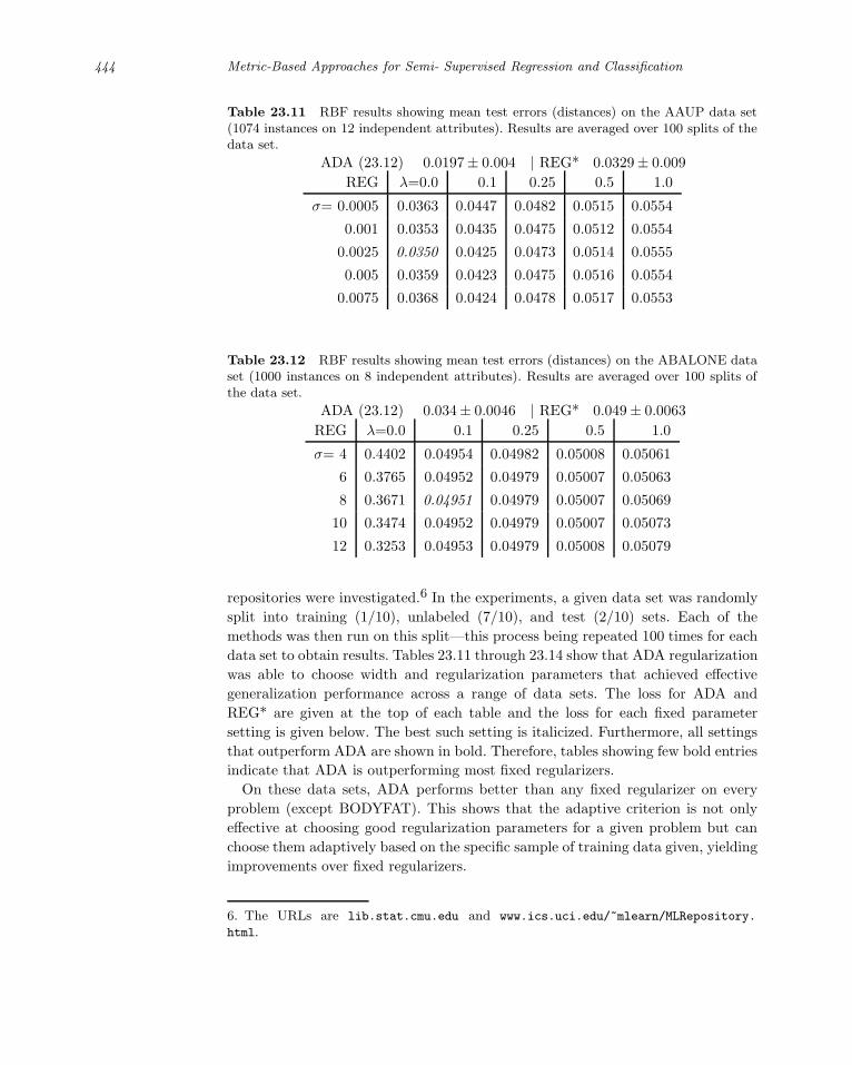
444 Metric-Based Approaches for Semi- Supervised Regression and Classification
Table 23.11 RBF results showing mean test errors (distances) on the AAUP data set(1074 instances on 12 independent attributes). Results are averaged over 100 splits of thedata set.
ADA (23.12) 0.0197± 0.004 | REG* 0.0329± 0.009
REG λ=0.0 0.1 0.25 0.5 1.0
σ= 0.0005 0.0363 0.0447 0.0482 0.0515 0.0554
0.001 0.0353 0.0435 0.0475 0.0512 0.0554
0.0025 0.0350 0.0425 0.0473 0.0514 0.0555
0.005 0.0359 0.0423 0.0475 0.0516 0.0554
0.0075 0.0368 0.0424 0.0478 0.0517 0.0553
Table 23.12 RBF results showing mean test errors (distances) on the ABALONE dataset (1000 instances on 8 independent attributes). Results are averaged over 100 splits ofthe data set.
ADA (23.12) 0.034± 0.0046 | REG* 0.049 ± 0.0063
REG λ=0.0 0.1 0.25 0.5 1.0
σ= 4 0.4402 0.04954 0.04982 0.05008 0.05061
6 0.3765 0.04952 0.04979 0.05007 0.05063
8 0.3671 0.04951 0.04979 0.05007 0.05069
10 0.3474 0.04952 0.04979 0.05007 0.05073
12 0.3253 0.04953 0.04979 0.05008 0.05079
repositories were investigated.6 In the experiments, a given data set was randomly
split into training (1/10), unlabeled (7/10), and test (2/10) sets. Each of the
methods was then run on this split—this process being repeated 100 times for each
data set to obtain results. Tables 23.11 through 23.14 show that ADA regularization
was able to choose width and regularization parameters that achieved effective
generalization performance across a range of data sets. The loss for ADA and
REG* are given at the top of each table and the loss for each fixed parameter
setting is given below. The best such setting is italicized. Furthermore, all settings
that outperform ADA are shown in bold. Therefore, tables showing few bold entries
indicate that ADA is outperforming most fixed regularizers.
On these data sets, ADA performs better than any fixed regularizer on every
problem (except BODYFAT). This shows that the adaptive criterion is not only
effective at choosing good regularization parameters for a given problem but can
choose them adaptively based on the specific sample of training data given, yielding
improvements over fixed regularizers.
6. The URLs are lib.stat.cmu.edu and www.ics.uci.edu/~mlearn/MLRepository.
html.

23.5 Classification 445
Table 23.13 RBF results showing mean test errors (distances) on the BODYFAT dataset (252 instances on 14 independent attributes). Results are averaged over 100 splits ofthe data set.
ADA (23.12) 0.131± 0.0171 | REG* 0.125 ± 0.0151
REG λ=0.0 0.1 0.25 0.5 1.0
σ= 0.1 0.1658 0.1299 0.1325 0.1341 0.1354
0.5 0.1749 0.1294 0.1321 0.1337 0.1352
1 0.1792 0.1294 0.1321 0.1336 0.1353
2 0.1837 0.1296 0.1322 0.1337 0.1356
4 0.1883 0.1299 0.1323 0.1339 0.1362
Table 23.14 RBF results showing mean test errors (distances) on the BOSTON-C dataset (506 instances on 12 independent attributes). Results are averaged over 100 splits ofthe data set.
ADA (23.12) 0.150± 0.0212 | REG* 0.151 ± 0.0197
REG λ=0.0 0.1 0.25 0.5 1.0
σ= 0.075 0.1619 0.15785 0.1614 0.1645 0.1679
0.1 0.1624 0.15779 0.1614 0.1645 0.1679
0.15 0.1633 0.15776 0.1615 0.1646 0.1680
0.2 0.1642 0.15777 0.1615 0.1647 0.1682
0.25 0.1649 0.15780 0.1616 0.1648 0.1683
23.5 Classification
The regularization approach developed in this chapter can also be applied to
classification problems. For classification, the label set Y is usually a small dis-
crete set and prediction error is typically measured by the misclassification loss,
err(y, y) = 1(y =y). With this loss function, distances are measured by the disagree-
ment probability d(f, g) = PX(f(x) = g(x)) (Ben-David et al., 1995). Using this
metric, the generic regularization objective from Eq. 23.12 can be directly applied to
classification problems. As it turns out, a direct application of our approach to this
case gives poor results (Schuurmans and Southey, 2002). An intuitive explanation
for this weakness is that classification functions are essentially histogram-like (i.e.,
piecewise constant), and this tends to limit the ability of unlabeled data to detect
erratic behavior off the labeled training sample. A recent generalization analysis
by Kaariainen and Langford (Kaariainen, 2005; Kaariainen and Langford, 2005)
suggests that effective model selection strategies might be achieved by using tight
generalization bounds derived from unlabeled data as a complexity penalizer. This
idea has yet to be investigated in detail, however. Rather than pursue modified tech-
niques for classification here, we instead consider a straightforward regression-based

446 Metric-Based Approaches for Semi- Supervised Regression and Classification
approach for the remainder of this chapter.
A natural alternative to misclassification loss exists for the subset of classification
methods that return a distribution over class labels instead of a single class label.
With these methods, Kullback-Leibler (KL) divergence (Cover and Thomas, 1991)
can be used instead of distance metrics to compare hypothesis functions with the
origin function φ.7 With such a distance, penalized training objectives8 can be
derived similar to Eqs. 23.11 and 23.12, the terms of which are
d(φ‖h) =1
u
n∑
i=l+1
φ(xi) logφ(xi)
h(xi)+ (1 − φ(xi)) log
1 − φ(xi)
1 − h(xi), (23.15)
d(φ‖h) =1
l
l∑
i=1
φ(xi) logφ(xi)
h(xi)+ (1 − φ(xi)) log
1 − φ(xi)
1 − h(xi), (23.16)
d(PY|X‖h) =1
l
l∑
i=1
−yi log h(xi) − (1 − yi) log(1 − h(xi)). (23.17)
Experiments were run on three classifiers that return class-membership probabil-
ities. The ADA penalization strategy was tested on logistic regression (LR) (Hastie
et al., 2001), kernel logistic regression (KLR) (Hastie and Tibshirani, 1990), and a
neural network (NN) (Hastie et al., 2001). Experiments were run on the two data
sets used throughout this book and on a set of UCI data sets. The LR prediction
function h is
h(x) =1
1 + e−wT x. (23.18)
The prediction functions for KLR and neural networks are closely related in
the experiments presented here. KLR simply kernalizes Eq. 23.18. For the neural
network used here, the activation function in the first layer is tanh(), and the output
layer uses the logistic function in Eq. 23.18. The ADA-penalized objectives for all
three are therefore very similar.
In all cases, gradient descent was used to optimize the ADA objective. We
compare against regularized versions of LR, using the penalty term λwT w, 0 ≤λ. All experiments were repeated ten times, and the average log-loss test error
reported. Ten labeled training points and 100 unlabeled points were used during
training, and the remaining points were used for testing.
The results for LR on most of the book data sets (cf. chapter 21) are shown in
table 23.15 for a variety of λ settings. (A binary version of COIL, called COIL0,1,
was used; SecStr and Text were omitted due to excessive size and dimensionality,
7. Note that KL divergence is not a proper distance metric but it is frequently used insuch contexts.8. For the sake of simplicity, only binary classification is considered.

23.5 Classification 447
respectively.) The results show that ADA-penalized LR is competitive on Digit1,
and beats the best fixed regularizer on the other sets. Results on six UCI data sets
(AUSTRALIAN, CRX, DIABETES, FLARE, GERMAN, and PIMA) are shown in
table 23.16. Again, results are competitive, coming close to the best fixed regularizer
in most cases and surpassing it on two data sets.
Table 23.15 Logistic regression (LR) results for six book data sets showing mean testingerror (log-loss) for ADA and regularized LR with various settings of λ.
Digit1 USPS COIL0,1 BCI g241c g241d
ADA 0.653 0.379 0.687 0.325 0.042 0.188
λ = 0 0.570 1.006 18.89 2.788 0.982 1.042
0.1 0.502 0.621 4.765 1.607 0.692 0.734
0.5 0.537 0.524 4.142 1.254 0.667 0.696
1.0 0.568 0.494 3.878 1.120 0.660 0.684
2.0 0.606 0.472 3.617 1.001 0.655 0.675
5.0 0.655 0.459 3.278 0.874 0.653 0.667
10.0 0.682 0.460 3.026 0.804 0.654 0.664
Table 23.16 Logistic regression (LR) results for six UCI data sets showing mean testingerror for ADA and regularized LR with various settings of λ.
AUST. CRX DIAB. FLARE GERM. PIMA
ADA 0.697 0.716 0.703 0.541 0.697 0.683
λ = 0 1.240 1.176 1.282 1.741 0.710 1.442
0.1 0.927 0.797 0.785 0.833 0.715 0.881
0.5 0.814 0.707 0.733 0.618 0.715 0.773
1.0 0.773 0.689 0.716 0.572 0.713 0.739
2.0 0.742 0.679 0.703 0.546 0.710 0.715
5.0 0.715 0.676 0.694 0.533 0.703 0.697
10.0 0.704 0.678 0.691 0.531 0.697 0.692
Similar experiments were run on kernel logistic regression using a Gaussian
kernel and a variety of settings for the standard deviation, σ. Results are shown

448 Metric-Based Approaches for Semi- Supervised Regression and Classification
in table 23.17 for the book data sets 9 and in table 23.18 for the UCI data. Like
the earlier regression results, the best fixed parameter setting is italicized and all
settings that outperform ADA are shown in bold.
On the book data, the results are excellent, beating the oracle regularizer on all
but Digit1 and coming very close even there. On the UCI data, the results are
more mixed but still quite positive. While the oracle is not surpassed on any data
set, ADA is still better than many fixed regularizers.
Table 23.17 Kernel logistic regression (KLR) results for six book data sets showingmean testing error for ADA and regularized KLR with various settings of λ and σ.
Digit1 ADA 0.518
σ = 0.1 0.5 1 5 10
λ = 0 0.693 0.691 0.572 0.569 0.701
0.1 0.693 0.692 0.636 0.690 0.723
0.5 0.693 0.693 0.667 0.716 0.725
1.0 0.693 0.693 0.677 0.718 0.724
2.0 0.693 0.693 0.684 0.717 0.721
5.0 0.693 0.693 0.689 0.712 0.715
10.0 0.693 0.693 0.691 0.706 0.709
USPS ADA 0.456
σ = 0.1 0.5 1 5 10
λ = 0 0.693 0.693 0.691 0.478 0.480
0.1 0.693 0.693 0.692 0.444 0.477
0.5 0.693 0.693 0.693 0.481 0.498
1.0 0.693 0.693 0.693 0.503 0.504
2.0 0.693 0.693 0.693 0.531 0.511
5.0 0.693 0.693 0.693 0.578 0.526
10.0 0.693 0.693 0.693 0.615 0.549
COIL0,1 ADA 0.685
σ = 0.1 0.5 1 5 10
λ = 0 0.693 0.693 0.693 0.693 0.693
0.1 0.693 0.693 0.693 0.693 0.693
0.5 0.693 0.693 0.693 0.693 0.693
1.0 0.693 0.693 0.693 0.693 0.693
2.0 0.693 0.693 0.693 0.693 0.693
5.0 0.693 0.693 0.693 0.693 0.693
10.0 0.693 0.693 0.693 0.693 0.693
BCI ADA 0.580
σ = 0.1 0.5 1 5 10
λ = 0 0.693 0.693 0.693 0.811 1.045
0.1 0.693 0.693 0.693 0.710 0.769
0.5 0.693 0.693 0.693 0.697 0.731
1.0 0.693 0.693 0.693 0.695 0.721
2.0 0.693 0.693 0.693 0.694 0.713
5.0 0.693 0.693 0.693 0.693 0.704
10.0 0.693 0.693 0.693 0.693 0.698
g241c ADA 0.513
σ = 0.1 0.5 1 5 10
λ = 0 0.693 0.693 0.693 0.693 0.754
0.1 0.693 0.693 0.693 0.693 0.701
0.5 0.693 0.693 0.693 0.693 0.695
1.0 0.693 0.693 0.693 0.693 0.694
2.0 0.693 0.693 0.693 0.693 0.693
5.0 0.693 0.693 0.693 0.693 0.693
10.0 0.693 0.693 0.693 0.693 0.693
g241d ADA 0.514
σ = 0.1 0.5 1 5 10
λ = 0 0.693 0.693 0.693 0.693 0.736
0.1 0.693 0.693 0.693 0.693 0.697
0.5 0.693 0.693 0.693 0.693 0.693
1.0 0.693 0.693 0.693 0.693 0.693
2.0 0.693 0.693 0.693 0.693 0.693
5.0 0.693 0.693 0.693 0.693 0.693
10.0 0.693 0.693 0.693 0.693 0.693
Finally, we present results on three unregularized neural networks, with three,
five, and ten hidden units respectively. Results for the book data are shown in
table 23.19 and for the UCI data in table 23.20. The results against unregularized
9. We presume the similar scores achieved by so many of the fixed regularizes on the bookdata are due to some regularity in those data.

23.6 Conclusion 449
Table 23.18 Kernel logistic regression (KLR) results for six UCI data sets showingmean testing error for ADA and regularized KLR with various settings of λ and σ.
AUSTRALIAN ADA 0.685
σ = 0.1 0.5 1 5 10
λ = 0 0.851 0.772 0.748 0.708 0.710
0.1 0.670 0.681 0.682 0.705 0.705
0.5 0.653 0.671 0.682 0.703 0.705
1.0 0.654 0.671 0.683 0.702 0.704
2.0 0.658 0.673 0.685 0.701 0.703
5.0 0.667 0.674 0.685 0.697 0.699
10.0 0.675 0.677 0.685 0.694 0.696
CRX ADA 1.111
σ = 0.1 0.5 1 5 10
λ = 0 1.141 1.153 1.033 0.946 0.851
0.1 0.770 0.826 0.826 0.830 0.787
0.5 0.703 0.760 0.779 0.798 0.779
1.0 0.689 0.739 0.762 0.784 0.772
2.0 0.681 0.721 0.744 0.767 0.762
5.0 0.679 0.700 0.720 0.742 0.742
10.0 0.682 0.690 0.704 0.723 0.725
DIABETES ADA 0.666
σ = 0.1 0.5 1 5 10
λ = 0 0.683 0.897 0.933 0.744 0.694
0.1 0.683 0.638 0.692 0.685 0.686
0.5 0.688 0.619 0.658 0.680 0.687
1.0 0.690 0.623 0.649 0.678 0.685
2.0 0.691 0.633 0.645 0.675 0.681
5.0 0.692 0.652 0.645 0.669 0.674
10.0 0.693 0.666 0.652 0.666 0.670
FLARE ADA 0.540
σ = 0.1 0.5 1 5 10
λ = 0 0.700 0.660 0.652 0.646 0.473
0.1 0.656 0.636 0.558 0.465 0.474
0.5 0.667 0.656 0.592 0.468 0.481
1.0 0.675 0.667 0.616 0.474 0.483
2.0 0.682 0.677 0.639 0.482 0.485
5.0 0.688 0.686 0.664 0.500 0.494
10.0 0.690 0.689 0.676 0.526 0.511
GERMAN ADA 0.804
σ = 0.1 0.5 1 5 10
λ = 0 0.968 1.480 1.574 0.888 0.720
0.1 0.717 0.814 0.845 0.680 0.640
0.5 0.683 0.699 0.716 0.640 0.633
1.0 0.682 0.678 0.683 0.632 0.633
2.0 0.684 0.669 0.664 0.628 0.633
5.0 0.688 0.670 0.657 0.628 0.634
10.0 0.690 0.676 0.661 0.632 0.636
PIMA ADA 0.680
σ = 0.1 0.5 1 5 10
λ = 0 0.678 0.906 0.818 0.714 0.684
0.1 0.679 0.646 0.679 0.683 0.682
0.5 0.686 0.636 0.670 0.680 0.681
1.0 0.688 0.641 0.666 0.679 0.679
2.0 0.690 0.648 0.663 0.677 0.678
5.0 0.692 0.661 0.661 0.673 0.674
10.0 0.693 0.672 0.664 0.671 0.671
neural networks are striking, dramatically reducing the tendency to overfit, even
as the model complexity increases (performance on the PIMA data set with ten
hidden nodes is the only notable anomaly to be found).
Overall, these results show considerable promise for the use of ADA with prob-
abilistic classifiers, but there are clearly improvements still to be made. Adapting
the technique to work with discrete classifiers also remains a key challenge.
23.6 Conclusion
A new approach to the classical complexity-control problem has been introduced
that is based on the intrinsic geometry of the function-learning task. This geometry
is exploited in such a way as to be able to incorporate information from both labeled
and unlabeled data in a semi-supervised learning task. Unlike the majority of such

450 Metric-Based Approaches for Semi- Supervised Regression and Classification
Table 23.19 Neural network (NN) results for the book data sets (except set 6) showingmean testing error for ADA and unregularized NN with 3, 5, and 10 hidden nodes.
hidden=3 Digit1 USPS COIL0,1 BCI g241c g241d
ADA 0.756 0.579 11.282 1.162 2.120 1.108
unreg NN 84.567 51.020 22.769 154.388 122.308 160.653
hidden=5 Digit1 USPS COIL0,1 BCI g241c g241d
ADA 0.829 1.422 2.998 1.324 30.349 3.108
unreg NN 77.577 47.166 41.629 165.090 151.790 139.809
hidden=10 Digit1 USPS COIL0,1 BCI g241c g241d
ADA 1.828 9.985 2.070 0.993 4.742 1.253
unreg NN 83.693 61.913 24.233 118.572 124.658 142.555
Table 23.20 Neural network (NN) results for six UCI data sets showing mean testingerror for ADA and unregularized NN with 3, 5, and 10 hidden nodes.
hidden=3 AUST. CRX DIAB. FLARE GERM. PIMA
ADA 0.90 0.78 2.45 0.64 0.64 0.93
unreg NN 34.40 79.53 13.95 40.73 0.64 8.87
hidden=5 AUST. CRX DIAB. FLARE GERM. PIMA
ADA 1.53 1.19 1.71 0.53 0.82 0.89
unreg NN 41.13 88.43 46.47 62.41 0.73 58.43
hidden=10 AUST. CRX DIAB. FLARE GERM. PIMA
ADA 1.09 1.33 2.10 0.72 1.03 11.64
unreg NN 110.13 48.96 30.23 80.88 13.89 55.94
techniques, this approach requires no assumptions about the relationship between
labeled and unlabeled data other than the key assumption that they are drawn
from the same probability distribution.
These new techniques seem to outperform standard approaches in a wide range
of regression problems and either outperform or are competitive with standard ap-
proaches in a range of classification problems, with only one comparatively weak
instance (ADA-regularized KLR). The primary source of this advantage is that
the proposed metric-based strategies are able to detect dangerous situations and
avoid making catastrophic overfitting errors while still being responsive enough
to adopt reasonably complex models when this is supported by the data. This
is accomplished by attending to the real distances between hypotheses. Stan-
dard complexity-penalization strategies completely ignore this information. Holdout
methods implicitly take some of this information into account, but do so indirectly
and less effectively than the metric-based strategies introduced here. Although there

23.6 Conclusion 451
is “no free lunch” in general (Schaffer, 1994) and a universal improvement cannot be
claimed for every complexity-control problem (Schaffer, 1993), one should be able
to exploit additional information about the task (i.e., knowledge of PX) to obtain
significant improvements across a wide range of problem types and conditions. The
empirical results support this view. Furthermore, ADJ remains very competitive
with newer model-selection techniques (Bengio and Chapados, 2003). Additionally,
ADJ has been independently extended along three lines (Chapelle et al., 2002): (i)
producing excellent results on time-series data, (ii) using estimated densities in lieu
of unlabeled data, and (iii) hybridizing ADJ with cross-validation.
An important direction for future research is to develop theoretical support for
these strategies—in particular, a stronger theoretical justification of the regulariza-
tion methods proposed in section 23.4, an improved analysis of the model selection
methods proposed in section 23.3, and investigation of how to apply the technique
in section 23.5 to a more general set of classifiers . It remains open as to whether
the proposed methods TRI, ADJ, and ADA are in fact the best possible ways to ex-
ploit the hypothesis distances provided by PX. A clear direction for future research
is the investigation of alternative strategies that could potentially be more effective
in this regard. For example, it remains for future work to extend the multiplicative
ADJ and ADA methods to cope with zero training errors. Additionally, more ex-
ploration of the effects of alternative origin functions (perhaps even ensembles of
origin functions) is necessary. Finally, it would be interesting to adapt the approach
to model combination methods, extending the ideas of Krogh and Vedelsby (1995)
to other combination strategies, including boosting (Freund and Schapire, 1997)
and bagging (Breiman, 1996).
Acknowledgments
Research was supported by the Alberta Ingenuity Centre for Machine Learning,
NSERC, MITACS, and the Canada Research Chair programme.


24 Transductive Inference and
Semi-Supervised Learning
Vladimir Vapnik [email protected]
This chapter discusses the difference between transductive inference and semi-
supervised learning. It argues that transductive inference captures the intrinsic
properties of the mechanism for extracting additional information from the unla-
beled data. It also shows an important role of transduction for creating noninductive
models of inference.1
24.1 Problem Settings
Let us start with the formal problem setting for transductive inference and semi-
supervised learning.
Transductive Inference: General Setting Given a set of ℓ training pairs,
(y1, x1), ...(yℓ, xℓ), xi ∈ Rd, yi ∈ −1, 1, (24.1)
and a sequence of k test vectors,
xℓ+1, ..., xℓ+k, (24.2)
find among an admissible set of binary vectors,
Y = (yℓ+1, ..., yℓ+k),
1. These remarks were inspired by the discussion, What is the Difference between Trans-ductive Inference and Semi-Supervised Learning?, that took place during a workshop closeto Tubingen, Germany (May 24, 2005).

454 Transductive Inference and Semi-Supervised Learning
the one that classifies the test vectors with the smallest number of errors. Here we
consider
x1, ..., xℓ+k (24.3)
to be random i.i.d. vectors drawn according to the same (unknown) distribution
P (x). The classifications y of the vectors x are defined by some (unknown) condi-
tional probability function P (y|x).
Below we will call the vectors (24.3) from the training and test sets the working
set of vectors.
Transductive Inference: Particular Setting In this setting the set of admis-
sible vectors is defined by the admissible set of indicator functions f(x, α), α ∈ Λ.
In other words, every admissible vector of classification Y∗ is defined as follows:
Y∗ = (f(x1, α∗), ..., f(xk, α∗)) .
Semi-Supervised Learning Given a set of training data (24.1) and a set of
test data (24.2), find among the set of indicator functions f(x, α), α ∈ Λ, the one
that minimizes the risk functional
R(α) =
∫|y − f(x, α)|dP (x, y). (24.4)
Therefore, in transductive inference the goal is to classify the given u test vectors
of interest while in semi-supervised learning the goal is to find the function that
minimizes the functional (24.4) (the expectation of the error).
Semi-supervised learning can be seen as being related to a particular setting of
transductive learning. Indeed, if one chooses the function to classify the given test
data (24.2) well, why not also use it to classify new unseen data? This looks like a
reasonable idea.
However from a conceptual point of view, transductive inference contains im-
portant elements of a new philosophy of inference and this is the subject of these
remarks.
The transductive mode of inference was introduced in the mid-1970s. It attempts
to estimate the values of an unknown function f(x, α0) at particular points of
interest. On the other hand, inductive inference attempts to estimate the unknown
function over its entire domain of definition (Vapnik, 2006). In the late 1970s the
advantage of transductive inference over inductive inference was shown on real life
problems (Vapnik and Sterin, 1977).
The problem of semi-supervised learning was introduced in the mid-1990s (cf. sec-
tion 1.1.3) and became popular in the early 2000s (Zhou et al., 2004).

24.2 Problem of Generalization in Inductive and Transductive Inference 455
24.2 Problem of Generalization in Inductive and Transductive Inference
The mechanism that provides the transductive mode of inference with an advantage
over the inductive mode in classification of the given points of interest has been
understood since the very first theorems of Vapnik-Chervonenkis (VC) theory were
proved.
Suppose that our goal is to find the function that minimizes the functional (24.4).
Since the probability measure in (24.4) is unknown we minimize the empirical risk
functional
Remp(α) =
ℓ∑
i=1
|yi − f(xi, α)| (24.5)
instead of the risk functional (24.4).
It was shown in (Vapnik and Chervonenkis, 1991), that the necessary and
sufficient conditions for consistency (as ℓ increases) of the obtained approximations
is the existence of the uniform convergence of frequencies (defined by (24.5)) to
their probabilities (defined by (24.4)) over a given set of functions f(x, α), α ∈ Λ:
P
sup
α|R(α) − Remp(α)| ≥ ε
−→ 0, ∀ε > 0. (24.6)
In 1968 the necessary and sufficient conditions for uniform convergence (24.6)
were discovered (Vapnik and Chervonenkis, 1968, 1971). They are based on the so-
called capacity factors. These factors will play an important role in our discussion.
We now introduce them.
24.2.1 The VC Entropy, Growth Function, and VC Dimension
Given a set of indicator functions f(x, α), α ∈ Λ and set of ℓ i.i.d. input vectors
x1, ..., xℓ, (24.7)
consider the value ∆Λ(x1, ..., xℓ) that defines the number of different classifications
of the set of vectors (24.7) using indicator functions from the set f(x, α), α ∈ Λ.
This is the number of equivalence classes2 of functions on which the set of vectors
(24.7) factorizes the set of functions f(x, α), α ∈ Λ. The number of equivalence
classes has the trivial bound
∆Λ(x1, ..., xℓ) ≤ 2ℓ. (24.8)
Using the value ∆Λ(x1, ..., xℓ) we define the following three capacity concepts.
2. A subset of functions that classify vectors (24.7) in the same way belong to the sameequivalence class (with respect to (24.7)).

456 Transductive Inference and Semi-Supervised Learning
1. The expectation of the number of equivalence classes,
∆ΛP (ℓ) = Ex1,...,xℓ
∆(x1, ..., xℓ), (24.9)
where the expectation is taken over i.i.d. data (24.7) drawn according to the
distribution P (x).
The function
HΛP (ℓ) = ln ∆Λ
P (ℓ) (24.10)
forms the first capacity concept. It is called the (annealed) VC entropy.3
The VC entropy depends on three factors:
(a) the set of functions f(x, α), α ∈ Λ,
(b) the number of vectors ℓ, and
(c) the probability measure P (x).
The condition
limℓ−→∞
HΛP (ℓ)
ℓ= 0 (24.11)
forms the necessary and sufficient condition for uniform convergence (24.6) for the
fixed probability measure P (x).
2. The second capacity concept is called the growth function. It is defined as
GΛ(ℓ) = maxx1,...,xℓ
∆Λ(xi, ..., xℓ). (24.12)
The value of the growth function depends on two factors:
a. the set of functions f(x, α), α ∈ Λ, and
b. the number of observations ℓ.
The condition
limℓ−→∞
lnGΛ(ℓ)
ℓ= 0 (24.13)
forms the necessary and sufficient condition for uniform convergence that is inde-
pendent of the probability measure (for all probability measures).
3. The third capacity concept is called the VC dimension.4
We say that a set of functions f(x, α), α ∈ Λ has VC dimension h if the largest
number ℓ for which the equality
GΛ(ℓ) = 2ℓ (24.14)
holds true is equal to h. If this equality is true for any ℓ we say that the VC
3. The abbreviation for Vapnik-Chervonenkis entropy.4. The abbreviation for Vapnik-Chervonenkis dimension.
24.3 Structure of the VC Bounds and Transductive Inference 457
dimension equals infinity. In other words
h = maxℓ
ℓ : GΛ(ℓ) = 2ℓ. (24.15)
The VC dimension depends only on one factor: (a) the set of functions. VC
dimension characterizes the diversity of this set of functions.
A finite VC dimension is the necessary and sufficient condition for uniform conver-
gence which is independent of the probability measure.
In 1968 we proved the important bound (Vapnik and Chervonenkis, 1968)
lnGΛ(ℓ) ≤ h
(ln
ℓ
h+ 1
). (24.16)
This bound allows one to upper-bound the growth function with a standard function
that depends on one parameter, the VC dimension.
We have therefore obtained the following relationship:
HΛP (ℓ) ≤ lnGΛ(ℓ) ≤ h
(ln
ℓ
h+ 1
). (24.17)
24.3 Structure of the VC Bounds and Transductive Inference
One of the key results of VC theory is the following bound:
P
sup
α|R(α) − Remp(α)| ≥ ε
≤ expHΛ
P (2ℓ) − ε2ℓ. (24.18)
One can rewrite this expression in the following form: with probability 1 − η
simultaneously for all α the inequality
R(α) ≤ Remp(α) +
√HΛ
P (2ℓ) − ln η
ℓ(24.19)
holds true. Note that this inequality depends on the distribution function P (x).
Since this inequality is true simultaneously for all functions of the admissible set,
the function that minimizes the right-hand side of (24.19) provides the guaranteed
minimum for the expected loss (24.4).
Taking into account (24.17) one can upper-bound (24.19) using the second
capacity concept, the growth function:
R(α) ≤ Remp(α) +
√lnGΛ(2ℓ) − ln η
ℓ. (24.20)
This bound is true for any distribution function (i.e. for the worst distribution
function). However it is less accurate (for a specific case P (x)) than (24.19).
One can also upper-bound (24.19) and (24.20) using the third capacity concept,

458 Transductive Inference and Semi-Supervised Learning
the VC dimension
R(α) ≤ Remp(α) +
√h(ln 2ℓ
h + 1) − ln η
ℓ. (24.21)
The good news about this bound is that it depends on just one parameter h and
not on some integer function GΛ(ℓ). However (24.21) is less accurate than (24.20)
which is less accurate than (24.19).
Transductive inference was inspired by the idea of finding better solutions using
the more accurate bound (24.19) instead of the bounds (24.20) and (24.21) used in
inductive inference.
24.4 The Symmetrization Lemma and Transductive Inference
Bounds (24.18) and (24.19) were obtained using the so-called symmetrization
lemma.
Lemma. The following inequality holds true:
P
sup
α|R(α) − Remp(α)| ≥ ε
≤ 2P
sup
α
∣∣∣R(1)emp(α) − R(2)
emp(α)∣∣∣ >
ε
2
, (24.22)
where
R(1)emp(α) =
1
ℓ
ℓ∑
i=1
|yi − f(xi, α)| (24.23)
and
R(2)emp(α) =
1
ℓ
2ℓ∑
i=ℓ+1
|yi − f(xi, α)| (24.24)
are the empirical risk functionals constructed using two different samples.
The bound (24.18) was obtained as an upper-bound of the right-hand side of
(24.22).
Therefore, from the symmetrization lemma it follows that to obtain a bound for
inductive inference we first obtained a bound for transductive inference (for the
right-hand side of (24.22)) and then upper-bounded that.
It should be noted that since the bound (24.18) was introduced in 1968, a
lot of efforts were made to improve it. However in all attempts the key element
remained the symmetrization lemma. That is, in all proofs of the bounds for
uniform convergence the first (and most difficult) step was to obtain the bound
for transductive inference. The trivial upper bound of this bound gives the desired
result.
This means that transductive inference is a fundamental step in machine learning
theory.
To get the bound (24.18) let us bound the right-hand side of (24.22). Two

24.5 Bounds for Transductive Inference 459
fundamental ideas were used to obtain this bound:
1. The following two models are equivalent: (a) one chooses two i.i.d. sets:5
x1, ..., xℓ, and xℓ+1, ..., x2ℓ;
(b) one chooses an i.i.d. set of size 2ℓ and then randomly splits it into two subsets
of size ℓ.
2. Using model (b) one can rewrite the right-hand side of (24.22) as follows:
Psupα
∣∣∣R(1)emp(α) − R
(2)emp(α)
∣∣∣ > ε2
=
Ex1,...,x2ℓP
supα |R(1)emp(α) − R
(2)emp(α)| > ε
2 | x1, ..., x2ℓ
.(24.25)
To obtain the bound we first bound the conditional probability,
Psupα |R(1)
emp(α) − R(2)emp(α)| > ε
2 | x1, ..., x2ℓ≤
∆Λ(x1, ..., x2ℓ) exp−ε2ℓ
,
(24.26)
and then take the expectation over working sets of size 2ℓ. As a result, we obtain
Ex1,...,x2ℓP
supα
∣∣∣R(1)emp(α) − R
(2)emp(α)
∣∣∣ > ε2
≤
E∆ΛP (2ℓ) exp
−ε2ℓ
= exp
HΛ
P (2ℓ) − ε2ℓ
.(24.27)
This bound depends on the probability measure P (x) (it contains the term HΛP (2ℓ)).
To obtain a bound which is independent of the probability measure we upper-bound
HΛP (2ℓ) by GΛ(2ℓ) (see (24.17)). Since GΛ(2ℓ) is independent of the probability
measure we obtain the bound
P
sup
α|R(α) − Remp(α)| ≥ ε
≤ GΛ(2ℓ) exp
−ε2ℓ
(24.28)
on uniform convergence that is independent of the probability measure.
Therefore, from the symmetrization lemma and (24.17) we obtained the bound
(24.28). Note, however, that in order to obtain this bound we twice used a rough
estimate: the first time when we used the symmetrization lemma, and the second
time when we used the function GΛ(2ℓ) instead of the function HΛP (2ℓ).
24.5 Bounds for Transductive Inference
The inequality (24.26) is the key element for obtaining a VC bound for transductive
inference.
Indeed, this inequality is equivalent to the following one: with probability 1− η
5. For simplicity of the formulas we choose two sets of equal size.

460 Transductive Inference and Semi-Supervised Learning
simultaneously for all functions f(x, α), α ∈ Λ, the inequality
1
ℓ
2ℓ∑
i=ℓ+1
|yi − f(x, α)| ≤ℓ∑
i=1
|yi − f(x, α)| +√
ln ∆Λ(x1, ..., x2ℓ) − ln η
ℓ(24.29)
holds true, where probability is defined with respect to splitting the set x1, ..., x2ℓinto two subsets:
1. one that is used in the training set x1, ..., xℓ and
2. one that forms the test set xℓ+1, ..., x2ℓ.
Note that this concept of probability is different from the one defined for inductive
inference and which requires the i.i.d. distribution of the elements x1, ..., x2ℓ. The
concepts of probability will be equivalent if an element of the working set is
i.i.d. according to some unknown fixed probability distribution function. If it is not,
then all formal claims are still correct but the concept of probability is changing.
In this sense we discuss in section 24.11.1 the idea of adaptation in transductive
inference.
But even in the i.i.d. case the bound for transduction is more accurate than
(24.20) and (24.21) used in inductive inference. However, the main advantage
of transduction over induction appears when one implements the structural risk
minimization principle.
24.6 The Structural Risk Minimization Principle for Induction and Transduction
In the 1970s the structural risk minimization (SRM) principle was introduced.
Its goal was to find the function that minimizes the right-hand side of inequality
(24.19). In order to achieve this goal the following scheme was considered.
Prior to the appearance of the training set, the set of admissible functions is
organized as a structure. The nested subsets of functions (called the elements of
the structure) are specified:
S1 ⊂ S2 ⊂ ... ⊂ SB ⊂ S = f : f(x, α), α ∈ Λ, (24.30)
where subset Sk has a fixed capacity (say VC dimension h = k).
The minimization of the right-hand side of inequality (24.29) can then be per-
formed over two terms of the inequality. One first chooses the element of the struc-
ture (controlling the second term through the value of hk) and then the function
in the chosen element of the structure (controlling the first term).
It was shown that the SRM principle is strongly uniformly consistent (Devroye
et al., 1996), (Vapnik, 1998). This means that when the sample size ℓ increases,
the error of the function selected by the SRM principle converges toward the best
possible error. However in order to find a good solution using a finite (limited)
number of training examples one has to construct a (smart) structure which
reflects prior knowledge about the problem of interest. In creating such a structure
transductive inference offers some additional opportunities with respect to inductive

24.6 The Structural Risk Minimization Principle for Induction and Transduction 461
inference.
The SRM principle for transductive inference can be introduced as follows
(Vapnik, 2006): Prior to splitting the given working set x1, ..., x2ℓ into the two
subsets that define the elements of the training and test sets, one constructs the
structure on the finite number N = ∆Λ(x1, ..., x2ℓ) of equivalence classes F1, ..., FN
that are the result of factorization of the given set of functions over the given 2ℓ
vectors.6
Let such a structure be
S∗1 ⊂ S∗
2 ⊂, ...,⊂ S∗B ⊂ S∗ = F1, ..., FN, (24.31)
where the subset S∗k contains Nk equivalence classes of functions from f(x, α), α ∈
Λ.
The opportunity to construct a “smart” structure on the elements of the equiv-
alence classes is a key advantage of SRM for transductive inference over SRM for
inductive inference.
The new development in SRM for transductive inference comes from the con-
sideration of the different “sizes” of the equivalence classes. The idea of creating a
smart structure on the set of equivalence classes due to their size remains the hierar-
chical Bayesian approach. In this approach one can distinguish two (several) levels
of hierarchy: Suppose that we are given a priori information P (α) on the set of ad-
missible functions (before the set of vectors x1, ..., x2ℓ appear). After these vectors
appear one can calculate prior information for equivalence classes μ(F1), ..., μ(FN )
as an integral
μ(Fk) =
∫
Fk
dP (α).
Using this prior information one can construct a “smart” structure where the first
element contains N1 equivalence classes with the largest values μ(Fi), i = 1, ..., N ,
the second element contains N2 equivalence classes with the largest value μ(Fi),
and so on.
Note that for transductive inference the construction of such a structure for a
given working set is a prior process since we do not use both the split of our x
vectors into the training and test subsets, and information about the classification
of the training data.7
6. The functions that take the same values on the working set of vectors x1, ..., x2ℓ formone equivalence class (with respect to the working set).7. One can unify transductive and inductive inference as follows: In both cases one isgiven a set of functions defined on some space. One uses the training examples from thisspace to define the values of the function of interest for the whole space of definition of thefunction. The difference is that in transductive inference the space of interest is discrete(defined on the working set (24.3)) while in inductive inference it is R
d. One can conducta nontrivial analysis of the discrete space but not the space R
d. This defines the key factorof the advantage of transductive inference.

462 Transductive Inference and Semi-Supervised Learning
For any element Sk of the structure, simultaneously for all equivalence classes
belonging to this element, with probability 1−η the following inequality holds true:
1
ℓ
2ℓ∑
i=ℓ+1
|yi − Fr(xi)| ≤1
ℓ
ℓ∑
i=1
|yi − Fr(xi)|+√
lnNk − ln η
ℓ, Fr ∈ Sk. (24.32)
The probability is defined with respect to a random split of the set of vectors (24.3)
into two subsets: training and test vectors.8
Therefore, to minimize the number of errors on the test vectors (the left-hand
side of (24.32)) we have to choose the element of the structure Sk (it defines the
value of the second term in the right-hand side of (24.32)) and the equivalence class
belonging to this element (it defines the value of the first term in the right-hand
side of (24.32)).
24.7 Combinatorics in Transductive Inference
When constructing structures on the set of equivalence classes in discrete space one
can play combinatorial tricks. This is impossible when constructing a structure on
the set of functions defined in the whole space.
Suppose we are given a working set of size 2ℓ which forms our discrete space. Sup-
pose in this space we have N equivalence classes F1, ..., FN of functions f(x, α), α ∈Λ.
Consider 2ℓ new problems described by 2ℓ discrete spaces: S1, ...., S2ℓ, where the
discrete space Sr is defined by working vectors (24.3) from which we removed the
vector xr. For each of these spaces we can construct a set of equivalence classes
and a corresponding structure on this set. For each of these classes with probability
1 − η the inequality (24.32) holds true and therefore simultaneously for all 2ℓ + 1
problems the inequality (24.32) is true with probability 1 − (2ℓ + 1)η. Therefore
with probability 1 − η simultaneously for all 2ℓ + 1 problems the inequality
R1(Fsi ) ≤ Rs
2(Fsi ) +
√lnNs
k − ln η + ln(2ℓ + 1)
ℓ − 1, Fr ∈ Sk (24.33)
holds true, where the term ln(2ℓ + 1) is due to our combinatorial games with one
element of the working set. One can find an analogous bound for a combinatorial
game with k elements of the working set.
Combinatorial games allow one to introduce a very deep geometric concept of
equivalence classes (see (Vapnik, 2006, 1998) for details).
8. One can obtain a better bound (see (Vapnik, 1998)).

24.8 Measures of the Size of Equivalence Classes 463
Figure 24.1 The large-margin hyperplane obtained using only the training set does notbelong to the largest equivalence class defined on the working set.
24.8 Measures of the Size of Equivalence Classes
We have not yet discussed how to measure the size of equivalence classes. In this
section we will discuss two possibilities. We could either
1. use a measure that reflects the VC dimension concept for the set of linear (in a
feature space) indicator functions: the value of a margin for the equivalence class,
or
2. measure the size of equivalence classes using the most refined capacity concept:
the VC entropy.
Using the size of the margin for equivalence class. With the appearance
of support vector machines (SVMs) the important problem became the following:
given a working set of vectors (24.3) construct a structure on the equivalence classes
of linear functions.
Let us measure the size μ(Fi) of an equivalence class Fi by the value of the
corresponding margin.9 Any equivalence class separates working vectors (24.3) into
two classes. Let us find among the functions belonging to the equivalence class one
that has the largest distance (margin) to the closest vector of the set (24.3). We
use this distance as the measure μ(Fi) for the size of the equivalence class Fi. This
measure and how it differs from the SVM are illustrated in figure 24.1.
Using this concept of the size of an equivalence class the SVM transductive
algorithms were suggested Vapnik (2006).
9. There is a direct connection between the value of the margin and the VC dimensiondefined on the set of equivalence classes (see (Vapnik, 1998, chapter 8)).

464 Transductive Inference and Semi-Supervised Learning
The recommendation of SRM for transductive inference would be:
To classify test vectors (24.2) choose the equivalence class (defined on the working
set (24.3)) that classifies the training data well and has the largest value of the
(soft) margin.
This idea is widely used in constructing transductive SVM algorithms (see
chapter 6).
The universum concept: To construct a measure on the size of the equivalence
class based on the most refined capacity concept, the VC entropy, the following
idea was introduced in (Vapnik, 1998). Suppose that for a given working set of data
(24.3) we construct additionally a new set of data,
x∗1, ..., x
∗u, x∗ ∈ R
d, (24.34)
called the universum. Using the working set (24.3) we will create a set of equivalence
classes of functions, and using the universum (24.34) we will evaluate the size of
the equivalence classes.
The universum plays the role of prior information in Bayesian inference. It
describes our knowledge of the problem we are solving. There exist, however,
important differences between prior information in Bayesian inference and prior
information given by the universum. In Bayesian inference, prior information is
information about the relationship of the functions in the set of admissible functions
to the desired one. The universum is information about a relationship between the
working set and a set of possible problems. For example, for the digit recognition
problem it can be some vectors whose images resemble a digit. It defines a style of
digits for the recognition task.
Using the value of the VC entropy defined on the universum. Consider
now the set of equivalence classes defined by the working set (24.3). Let us measure
the size μ(Fk) of the equivalence class Fr by the value ln ∆Fr (x∗1, ..., x
∗v). This
defines the logarithm of the number of different separations of the vectors from
the universum (24.34) by the functions belonging to this equivalence class. This
measure defines the diversity of the functions from the equivalence class. The size
of the equivalence classes decreases with the index in the structure.
The recommendation of SRM for transductive inference would be:
To classify test vectors (24.2) choose the equivalence class (defined on the working
set (24.3)) that classifies the training data (24.1) well and has the largest value of
the VC entropy (the largest diversity) on the universum (24.34).
Using the number of contradictions on the universum. Unfortunately it
is not easy to estimate the values of the VC entropy of equivalence classes on the
universum. Therefore we simplify this measure. Let us consider the vector x∗i as one
that contradicts equivalence class Fr if in class Fr there are functions that classify
this vector as belonging to the first category as well as functions that classify x∗i as
belonging to the second category.
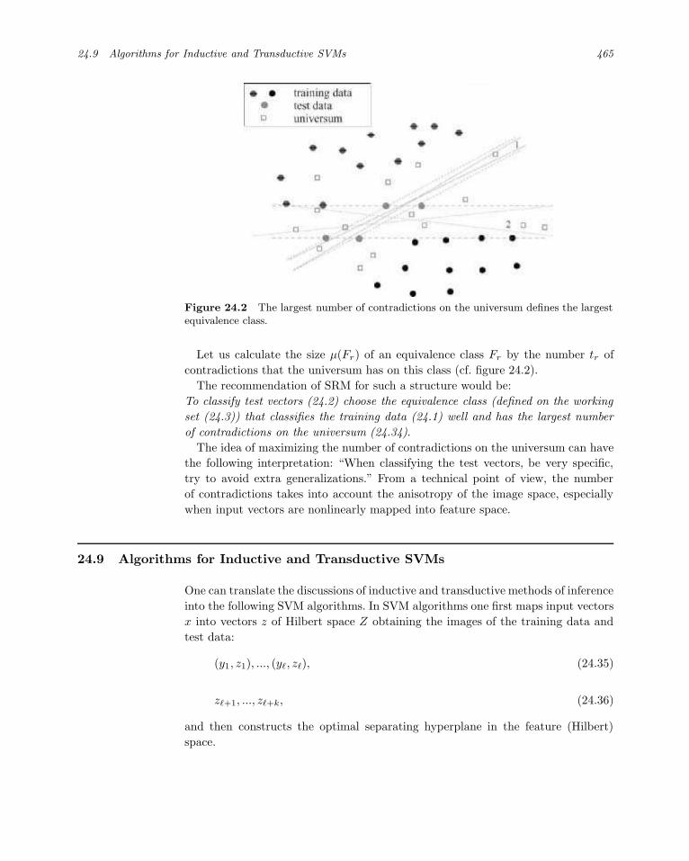
24.9 Algorithms for Inductive and Transductive SVMs 465
Figure 24.2 The largest number of contradictions on the universum defines the largestequivalence class.
Let us calculate the size μ(Fr) of an equivalence class Fr by the number tr of
contradictions that the universum has on this class (cf. figure 24.2).
The recommendation of SRM for such a structure would be:
To classify test vectors (24.2) choose the equivalence class (defined on the working
set (24.3)) that classifies the training data (24.1) well and has the largest number
of contradictions on the universum (24.34).
The idea of maximizing the number of contradictions on the universum can have
the following interpretation: “When classifying the test vectors, be very specific,
try to avoid extra generalizations.” From a technical point of view, the number
of contradictions takes into account the anisotropy of the image space, especially
when input vectors are nonlinearly mapped into feature space.
24.9 Algorithms for Inductive and Transductive SVMs
One can translate the discussions of inductive and transductive methods of inference
into the following SVM algorithms. In SVM algorithms one first maps input vectors
x into vectors z of Hilbert space Z obtaining the images of the training data and
test data:
(y1, z1), ..., (yℓ, zℓ), (24.35)
zℓ+1, ..., zℓ+k, (24.36)
and then constructs the optimal separating hyperplane in the feature (Hilbert)
space.

466 Transductive Inference and Semi-Supervised Learning
24.9.1 SVMs for Inductive Inference
Given the images (24.35) of the training data (24.1) construct the large-margin
linear decision rule (Vapnik, 1995):
I(x) = θ[(w, z) + b],
where the vector w and threshold b are the solution of the following convex quadratic
optimization problem: Minimize the functional
R(w) = (w, w) + C1
ℓ∑
i=1
θ(ξi), C1 ≥ 0 (24.37)
subject to the constraints
yi[(zi, w) + b] ≥ 1 − ξi, ξi ≥ 0, i = 1, ..., ℓ (24.38)
(defined by the images of the training data (24.35)) where we have denoted
θ(ξi) =
1, if ξi > 0
0, if ξi = 0.
24.9.2 SVMs for Inductive Inference Using the Universum
Given the images (24.35) of the training data (24.1), images (24.36) of the test data
(24.2), and the images
z∗1 , ..., z∗u (24.39)
of universum (24.34), construct the linear decision rule
I(x) = θ[(w, z) + b],
where the vector w and threshold b are the solution of the following convex quadratic
optimization problem: Minimize the functional
R(w) = (w, w) + C1
ℓ∑
i=1
θ(ξi) + C2
u∑
s=1
θ(ξ∗s ), C1, C2 ≥ 0 (24.40)
subject to the constraints
yi((zi, w) + b) ≥ 1 − ξi, ξi ≥ 0, i = 1, ..., ℓ (24.41)
(defined by the images of the training data (24.35)) and the constraints
|(z∗s , w) + b| ≤ a + ξ∗s , ξ∗s ≥ 0, s = 1, ..., u, a ≥ 0 (24.42)
defined by the images (24.39) of the universum (24.34).

24.9 Algorithms for Inductive and Transductive SVMs 467
24.9.3 SVM for Large-Margin Transductive Inference
Given the images (24.35) of the training data (24.1) and the images (24.36) of
the test data (24.2) construct the large-margin linear decision rule for transductive
inference,
I(x) = θ[(w, z) + b],
where the vector w and threshold b are the solution of the following optimization
problem: Minimize the functional
R(w) = (w, w) + C1
ℓ∑
i=1
θ(ξi) + C2
ℓ+k∑
j=ℓ+1
θ(ξj), C1, C2 ≥ 0 (24.43)
subject to the constraints
yi((zi, w) + b) ≥ 1 − ξi, ξi ≥ 0, i = 1, ..., ℓ (24.44)
(defined by the images (24.35) of the training data (24.1)) and the constraints
y∗j ((zj , w) + b) ≥ 1 − ξj , ξj ≥ 0, j = ℓ + 1, ..., ℓ + k (24.45)
(defined by the images (24.36) of the test data (24.2)) and its desired classifictions
y∗ℓ+1, ..., y
∗ℓ+k.
One more constraint. To avoid unbalanced solution, Capelle and Zien, following
ideas of Thorsten Joachims, suggested the following constraint (Chapelle and Zien,
2005)):
1
u
ℓ+k∑
j=ℓ+1
((w, zj) + b) ≈ 1
ℓ
ℓ∑
i=1
yi. (24.46)
This constraint requires that the test data have about the same proportion of
vectors from the two classes as was observed for the training data.
24.9.4 SVM for Transductive Inference Based on Contradictions on the
Universum
Given the images (24.35) of the training data (24.1), the images (24.36) of the test
data (24.2), and the images (24.39) of the universum (24.34), construct the linear
decision rule
I(x) = θ[(w, z) + b],

468 Transductive Inference and Semi-Supervised Learning
where the vector w and threshold b are the solution of the following optimization
problem: Minimize the functional
R(w) = (w, w)+C1
ℓ∑
i=1
θ(ξi)+C2
ℓ+k∑
j=ℓ+1
θ(ξj)+C3
u∑
s=1
θ(ξ∗s ), C1, C2, C3 ≥ 0 (24.47)
subject to the constraints
yi((zi, w) + b) ≥ 1 − ξi, ξi ≥ 0, i = 1, ..., ℓ (24.48)
(defined by the images of the training data (24.35)), the constraints
y∗j ((zj , w) + b) ≥ 1 − ξj , ξj ≥ 0, j = ℓ + 1, ..., ℓ + k (24.49)
(defined by the images of the test data (24.36)) and its desired classification, and
the constraints
|(z∗s , w) + b| ≤ a + ξ∗s , ξ∗s ≥ 0, s = 1, ..., v, a ≥ 0 (24.50)
(defined by the images (24.39) of the universum (24.34)).
24.9.5 Standard Implementation of the SVM Algorithms
To simplify the optimization problems of the described algorithms the step function
θ(ξ) was replaced by the linear function ξ in the objective functionals (24.37),
(24.40), (24.43), and (24.47). Therefore the following algorithms were obtained
(Vapnik, 1995, 1998):
Large-margin inductive SVM:
Minimize the functional
R(w) = (w, w) + C1
ℓ∑
i=1
ξi, C1 ≥ 0 (24.51)
subject to the constraints (24.38).
Large-margin inductive SVM with the universum
Minimize the functional
R(w) = (w, w) + C1
ℓ∑
i=1
ξi, +C2
u∑
s=1
ξ∗s , C1 ≥ 0 (24.52)
subject to the constraints (24.41) and (24.42).
Large-margin transductive SVM:
Minimize the functional
R(w) = (w, w) + C1
ℓ∑
i=1
ξi + C2
ℓ+u∑
j=ℓ+1
ξj , C1, C2 ≥ 0 (24.53)

24.9 Algorithms for Inductive and Transductive SVMs 469
Table 24.1 Test errors of SVMs trained without and with universum.
# of train. examples. 250 500 1,000 2,000 3,000
Test Err. SVM (%) 2.83 1.92 1.37 0.99 0.83
Test Err. SVM+U1 (%) 2.43 1.58 1.11 0.75 0.63
Test Err. SVM+U2 (%) 1.51 1.12 0.89 0.68 0.60
Test Err. SVM+U3 (%) 1.33 0.89 0.72 0.60 0.58
subject to the constraints (24.44) and (24.45). One can also use hint (24.46).
Maximal contradictions on the universum transductive SVM:
Minimize the functional
R(w) = (w, w) + C1
ℓ∑
i=1
ξi + C2
ℓ+k∑
j=ℓ+1
ξj + C3
u∑
s=1
ξ∗s , C1, C2, C3 ≥ 0 (24.54)
subject to the constraints (24.48), (24.49), (24.50). One can also use hint (24.46).
24.9.6 Experiments with the Universum
In the summer of 2005, R. Collobert and J. Weston conducted the first experiments
on training SVMs with a universum. They demonstrated that
a. SVMs plus a universum can significantly improve performance even in the
inductive mode (C2 = 0 in inequality (24.54));
b. for small training sets it is very important how the universum is constructed.
For large sets it is less important.
Using the NIST database they discriminated digit 8 from digit 5 using a conven-
tional SVM and an SVM trained with three different universum environments.
Table 24.1 shows for different sizes of training data the performance of conven-
tional SVMs and the performance of SVMs trained using universums U1, U2, U3. In
all cases the parameter a = .01, and the parameters C1, C2 and the parameter of
Gaussian kernel were tuned using the tenfold cross-validation technique.
For these experiments three different universums (each containing 5000 examples)
were constructed as follows:
U1 Select random digits from the other classes (0,1,2,3,4,6,7,9).
U2 Creates an artificial image by first selecting a random 5 and a random 8,
(from pool of 3,000 non-test examples) and then for each pixel of the artificial
image choosing with probability 1/2 the corresponding pixel from the image 5 or
from the image 8.
U3 Creates an artificial image by first selecting a random 5 and a random 8,
(from pool of 3,000 non-test examples) and then constructing the mean of these
two digits.

470 Transductive Inference and Semi-Supervised Learning
24.10 Semi-Supervised Learning
Analyzing the problem of semi-supervised learning as the minimization of the
functional (24.4) using training data (24.1) and unlabeled data (24.2), one has
to create a clear statistical model that allows one to show where (from the formal
point of view) one can expect to get an advantage using unlabeled data.
From the theoretical point of view such a statistical model for semi-supervised
learning would be more sophisticated than the one described for transductive infer-
ence, since it would require additional reasoning in the style of the symmetrization
lemma.
Also, from the point of view of possible mechanisms for generalization it looks
restricted: Density is defined in input space. It does not depend on the mapping from
the input space to the feature space. As we mentioned earlier, a nonlinear mapping
can create a large anisotropy in feature space. Using the universum one can take
into account this anisotropy, evaluating the size of equivalence classes and using
it for classification. If the results obtained in the digit recognition experiments are
more or less general, transductive inference can have a more interesting structure
than just taking into account density properties.
Therefore it might be a good idea to consider the semi-supervised model as a
particular transductive model described at the beginning of this chapter. As such,
one first chooses the best equivalence class to perform transductive inference and
then chooses from this equivalence class some function which one uses to classify
new data that do not belong to the working set.
Such a position allows one to concentrate on the core problem of extracting
additional information from the unlabeled data in order to classify them.
24.11 Conclusion: Transductive Inference and the New Problems of Inference
There are two reasons to consider the transductive mode of inference as we have
described it above. The first reason is that it is an extremely useful tool for practical
applications (see Weston et al. (2003b) and chapter 6).
24.11.1 Adaptation to the Test Data
Transductive inference also contains elements of adaptation to new data which we
did not discuss since it is not easy to formalize. Back in the 1970s in the very first
article devoted to the application of transductive inference (Vapnik and Sterin,
1977), we used data from one medical clinic to classify patients from another clinic.
Transduction significantly improved performance.
Another example would be zip code recognition where transductive inference
suggests simultaneously recognizing all digits of a zip code in contrast to recognizing
every digit separately as in inductive inference. It is easy to imagine a situation

24.12 Beyond Transduction: Selective Inference 471
where given the training data and an unknown zip code the recognition of any
fixed digit of a zip code depends on recognition of the rest of the digits of the
zip code. That is, the rule is constructed for the specific zip code. For another zip
code one constructs another rule (which might reflect the adaptation to different
handwriting). One can find many such examples.
24.12 Beyond Transduction: Selective Inference
The second reason for considering transductive inference is that it forms the
simplest model of noninductive inference. These inferences are based on the same
general model as inductive inference: the SRM principle. The theory of transduction
describes (in the framework of the SRM principle) the mechanisms that provide the
advantage of transductive inference over inductive inference.
There also exist models of inferences that go beyond transduction. In particular,
selective inference:
Given ℓ training examples,
(xi, y1), ..., (xℓ, yℓ), (24.55)
and u candidate vectors,
xℓ+1, ...xℓ+u, (24.56)
select among the u candidates the k vectors with the highest probability of
belonging to the first class. Examples of selective inference include:
Discovery of bioactive drugs: Given a training set (24.55) of bioactive and non-
bioactive drugs, select from the u candidates (24.56) the k representatives with the
highest probability of belonging to the bioactive group.
National security: Given training set (24.55) of terrorists and nonterrorists, select
from the u candidates (24.56) the k representatives with the highest probability of
belonging to the terrorist group.
Note that selective inference requires a less demanding solution than transductive
inference: it does not require classification of the most difficult (border) cases.
Selective inference is the basis for solving high-dimensional decision-making
problems. To analyze the selective inference problem one can use the same SRM
principle but with a different concept of equivalence classes.

472 Transductive Inference and Semi-Supervised Learning
24.12.1 Transductive Inference and the Imperative for Inference in a
Complex World
Lastly, the philosophy of transductive inference reflects the general imperative
for inference in a complex (high-dimensional) world (Vapnik, 1995), which in
fact defines an advantage of the predictive learning models (machine learning
techniques) with respect to the generative learning models (classical statistics
techniques) (cf. section 1.2.4):
Solving a problem of interest, do not solve a more general (and therefore worse-
posed) problem as an intermediate step. Try to get the answer that you really need
but not a more general one.
Do not estimate a density if you need to estimate a function.
(Do not use classical generative models; use ML predictive models.)
Do not estimate a function if you need to estimate values at given points.
(Try to perform transduction, not induction.)
Do not estimate predictive values if your goal is to act well.
(A good strategy of action can rely just on good selective inference.)

25 A Discussion of Semi-Supervised Learning
and Transduction
The following is a fictitious discussion inspired by real discussions between the
editors of this book and a number of people, including Vladimir Vapnik. It involves
three researchers; for simplicity, we will call them A, B, and C, without implying
any one-to-one mapping to real persons. The topic of the discussion is: What is the
Difference between Semi-Supervised and Transductive Learning?
A: Let me start by saying that to me, the topic of our discussion seems strange.
Rather than asking for the difference, we should ask what SSL1 and transduction
have in common, if anything. SSL is about how to use information contained in
unlabeled data which we have in addition to the labeled training set. Transduction,
on the other hand, claims that it is powerful because it is solving a simpler task
than inductive learning.
B: Exactly. In inductive learning, one learns a function that makes predictions on
the whole space. Transduction asks for less — it only concerns itself with predicting
the values of the function at the test points of interest. This is an easier problem,
since an inductive solution implies a transductive one — by evaluating the function
at the given test points — but not vice versa.
A: But couldn’t you easily build an inductive algorithm from a transductive one
by carrying out the following procedure? For all possible test inputs x: add x as a
single unlabeled point to the labeled training set, and use the transductive algorithm
to predict the corresponding output. This gives you a mapping from x to y, in other
words, a function, just like any inductive algorithm. So a transductive solution
implies an inductive one, and thus transduction is no easier than induction.
1. We use the shorthand SSL for semi-supervised learning.

474 A Discussion of Semi-Supervised Learning and Transduction
B: As soon as we have more than one unlabeled point, this argument fails.
Nevertheless, in order to retain the distinction between induction and transduction,
we may want to exclude the situation. Whatever it is called, even the case of one
unlabeled point is interesting: it could be viewed as induction with a function class
which is not given explicitly.
Transduction works because the test set can give you a nontrivial factorization
of the function class. Let us call two functions equivalent if they cannot be
distinguished based on any of the given training or test examples. It is then sufficient
to use only one representative of each equivalence class, and forget about all other
functions. Our function class is effectively finite, and we can directly write down a
generalization error bound.
By the way, the size of the equivalence classes is important for generalization: I
believe that functions from large classes generalize better. Think of the notion of a
margin: if you have a large margin of separation between two classes of data, then
there are usually many different functions that fit into this margin, and correctly
separate the data (and thus are equivalent on the data).
C: This seems an interesting point. You said that one point is not enough for
transduction — how about for SSL? Would one unlabeled point be of any use?
A: Every unlabeled point gives me information on P (x). Whether the point is
useful or not will of course depend on whether my distribution is benign. For
example, if the distribution satisfies the semi-supervised smoothness assumption,2
then even a single point gives me information. For instance, it affects my estimate
of the local density of the points, and thus it affects where I will try to enforce
smoothness. As a consequence, it affects my prediction of how the class label should
behave as a function of the input.
B: For transduction to work, it is not necessary to make smoothness assumptions.
C: But surely, the factorization of the function class which you talked about before
will also depend on P (x)?
B: Yes.
C: I think it should be possible to construct cases where large equivalence classes
generalize worse than small ones. So I would claim that transduction, the way you
view it, will not always work, but only if the data are benign in some sense...
2. See chapter 1.

A Discussion of Semi-Supervised Learning and Transduction 475
A: ... and I would argue that one notion that captures whether the data are benign
is the semi-supervised smoothness assumption. This also makes the connection with
the margin, since large-margin separation is low-density separation.
B: Maybe yes, maybe no.
C: And what happens toward the other extreme of an infinite number of points?
A: Usually, learning becomes easier if we have more points. With transduction,
the more test points we have, the closer we get to inductive learning, because we
will have to predict outputs for a set of points that eventually covers the whole
domain. According to B, transduction would then become harder, since induction
is harder. But that’s absurd — how can one make a problem harder by adding more
information?
C: Interesting point... However, I am tempted to defend B, albeit with an ar-
gument he may not like: In the limit of infinitely many test points, transduction
should converge toward something like “induction plus knowledge of P (x).” This
could well be statistically easier than standard supervised inductive learning, pro-
vided P (x) contains useful information for our task. Which brings us again to the
role of the smoothness assumption.
A: This seems to show that transduction relies on the same kind of assumptions
as SSL. And, for increasing amounts of unlabeled points, SSL also converges to
induction plus knowledge of P (x). So where is the difference? In the limit of
infinitely many unlabeled points, transduction cannot be easier than inductive SSL.
B: In the real world, we do not have infinitely many data points. Anyway, my
point of view is more fundamental. It is based on what is behind the VC bounds for
induction. To prove these bounds, one uses the symmetrization lemma — we upper-
bound the difference between the error on the training set and the expected error
by the error on the training sample and the error on a second sample — the ghost
sample. This is exact transduction; it is a statement about the error on a given set
of points. But the VC bounds for induction then have to take an expectation with
respect to the unknown points, or even a supremum over the choice of the points.
This is much worse than what one can do knowing the points.3
A: But a better bound does not necessarily imply a better algorithm..
B: True, but bounds guide us to design new algorithms. Transduction is a step
on the way, which lies at the heart of induction. It looks deeper than induction.
3. See chapter 24 and (Vapnik, 2006).

476 A Discussion of Semi-Supervised Learning and Transduction
C: But doesn’t this contradict the no-free-lunch theorem?
B: There might exist distributions for which transduction can give worse results
than induction.
A: If I try to sum up the arguments of B, there are two different reasons why
transduction can be useful. The first one is that the bounds for transduction are
tighter than the bounds for induction, and the second one is that measuring the size
of the equivalence classes is an opportunity to change the ordering in the structure
of our class of functions. This second reason seems closely related to the motivations
in SSL.
C: Maybe we should look at a more concrete issue: Is the “transductive SVM” an
example of a transductive algorithm?
A: No. It is semi-supervised and inductive. It uses unlabeled data, and it provides
a function defined everywhere. Would you agree, B?
B: Maybe it is semi-supervised. My point is that transduction is orthogonal from
SSL. SSL stresses new technical ideas while transduction stresses new philosophical
ideas related to noninductive inference. I am convinced that in ten years the concept
of noninductive inference will be much more popular than inductive inference.
A: I surely agree that the two notions are orthogonal, but for different reasons.
To make my point clear let me consider two sets. One of them is a set of unlabeled
data which we have for training. I don’t care about the predictions on this set, I
only care about how to use the information this set provides about P (x). So I need
to assume that this set actually comes from P (x), or at least from a distribution
that is related to P (x) in some way. The other set is the actual test set. I do not care
where it comes from; it could be anything. In my view, a transductive algorithm
is one whose solution depends on the test points that I am given. The opposite of
a transductive algorithm is an inductive one. A semi-supervised algorithm, on the
other hand, is one that depends on the unlabeled set (as opposed to a supervised
algorithm). It does not care which test points are used in the end to evaluate its
performance.
B: This does not make sense to me. The test points need to be meaningful.
Transduction is intrinsically simpler than induction: it does not make predictions
for arbitrary test points.

A Discussion of Semi-Supervised Learning and Transduction 477
A: Coming back to the idea of avoiding to solve a more complicated problem
than necessary, what about local learning?4 The idea behind it is that, given a test
point, one should focus on the training points which are in a neighborhood of this
test point, construct a local decision rule, and predict the label of the test point
according to this ad hoc rule. Isn’t it almost the same idea as in transduction?
B: Indeed, the philosophy is similar, since in both cases one solves a simpler
problem. However, local learning is still inductive because there exists an implicit
decision function, even though it is never explicitely constructed. The concept of
local learning is actually almost the same as transduction with one test point which
we were talking about earlier.
C: This local learning idea might also be present in TSVM. Indeed, I can see an
advantage in using as unlabeled points the test points rather than an arbitrary set
of unlabeled points: by doing so, the algorithm concentrates in the regions of the
space where it is important to be accurate, as in local learning.5
A: The way I view them, transductive algorithms can also be designed for
computational reasons. Take, for instance, the Bayesian committee machine.6 The
solution returned by this algorithm is an expansion on a set of basis functions.
But for computational efficiency, only basis functions centered at the test points
are considered. So the solution will depend on the test set and the algorithm is
transductive according to my definition...
C: ... but not according to the definition of B, since for this algorithm the test
points can be arbitrary.
A: If we cannot agree on a definition of transduction, maybe we can at least agree
on some examples of transductive algorithms?
C: Graph-based algorithms7 can be interpreted as both semi-supervised and
transductive. They are transductive because there is no straightforward way of
making a prediction on a test point which is not drawn from P (x). Indeed,
including that point in the graph could be harmful, since it may provide misleading
information about P (x). In transduction, the test points have to be from P (x), or
at least some distribution related to P (x).
4. See (Bottou and Vapnik, 1992).5. Some experimental evidence for this claim is presented in (Collobert et al., 2006).6. See (Tresp, 2000).7. See part III of the book.

478 A Discussion of Semi-Supervised Learning and Transduction
A: And this shows why transductive methods are always semi-supervised: they
use information contained in the test points. Otherwise there would be no reason
not to consider arbitrary test points.
B: I have a typical example of transductive learning. Consider zip code recogni-
tion: since all the digits have been written by the same person, one can gain by
trying to recognize all the digits simultaneously instead of one by one.
C: This is an interesting example. But it seems different from the standard i.i.d.
framework: in this case, if viewed as drawn from the distribution of all possible
digits, the test points are dependent, because they have been written by the same
person.
B: Indeed, and it is probably in this kind of situtation where transduction is most
useful: when the test points have some special structure.
A: I do not think we have resolved the question we were asking. Read chapter 25
of Chapelle et al. (2006) and the references therein, and you will understand what
I mean.

References
B. Abboud, F. Davoine, and M. Dang. Expressive face recognition and synthesis. In ComputerVision and Pattern Recognition Workshop, volume 5, page 54, 2003.
N. Abe, J. Takeuchi, and M. Warmuth. Polynomial learnability of stochastic rules with respect tothe KL-divergence and quadratic distance. IEICE Transactions on Information and Systems,E84-D(3):299–316, March 2001.
Y. S. Abu-Mostafa. Machines that learn from hints. Scientific American, 272(4):64–69, 1995.
A. K. Agrawala. Learning with a probabilistic teacher. IEEE Transactions on Information Theory,16:373–379, 1970.
A. Agresti. Categorical Data Analysis. Wiley, Hoboken, NJ, 2002.
H. Akaike. Statistical predictor information. Annals of the Institute of Statistical Mathematics,22:203–271, 1970.
H. Akaike. A new look at the statistical model identification. IEEE Transactions on AutomaticControl, 19:716–723, 1974.
B. Alberts, D. Bray, A. Johnson, J. Lewis, M. Raff, K. Roberts, and P. Walter. Essential CellBiology: An Introduction to the Molecular Biology of the Cell. New York, Garland SciencePublishing, 1998.
S. F. Altschul, W. Gish, W. Miller, E. W. Myers, and D. J. Lipman. A basic local alignmentsearch tool. Journal of Molecular Biology, 215:403–410, 1990.
S. F. Altschul, T. L. Madden, A. A. Schaffer, J. Zhang, Z. Zhang, W. Miller, and D. J. Lipman.Gapped BLAST and PSI-BLAST: A new generation of protein database search programs.Nucleic Acids Research, 25:3389–3402, 1997.
Y. Altun, D. McAllester, and M. Belkin. Maximum margin semi-supervised learning for structuredvariables. In Advances in Neural Information Processing Systems, volume 18, 2005.
M. R. Amini and P. Gallinari. Semi-supervised logistic regression. In Fifteenth EuropeanConference on Artificial Intelligence, pages 390–394, 2002.
J. A. Anderson. Multivariate logistic compounds. Biometrika, 66:17–26, 1979.
M. Anjos. New Convex Relaxations for the Maximum Cut and VLSI Layout Problems. Phdthesis, Waterloo University, Waterloo, Canada, 2001.
F. Bach, G. Lanckriet, and M. Jordan. Multiple kernel learning, conic duality, and the SMOalgorithm. In Proceedings of the Twenty-first International Conference on Machine Learning,New York, 2004. ACM Press.
R. Baeza-Yates and B. Ribeiro-Neto. Modern Information Retrieval. ACM Press, New York,1999.
M.-F. Balcan and A. Blum. A PAC-style model for learning from labeled and unlabeled data. InConference on Computational Learning Theory, pages 111–126, 2005.
M.-F. Balcan, A. Blum, and K. Yang. Co-training and expansion: Towards bridging theory andpractice. In Advances in Neural Information Processing Systems, 2004.
S. Baluja. Probabilistic modeling for face orientation discrimination: Learning from labeled andunlabeled examples. In Advances in Neural Information Processing Systems 11, pages 854–860,1999.
A. Banerjee, I. Dhillon, J. Ghosh, and S. Sra. Clustering on the unit hypersphere using vonMises-Fisher distributions. Journal of Machine Learning Research, 6:1345–1382, 2005a.
A. Banerjee, S. Merugu, I. Dhilon, and J. Ghosh. Clustering with Bregman divergences. Journalof Machine Learning Research, 6:1705–1749, Oct 2005b.

480 REFERENCES
N. Bansal, A. L. Blum, and S. Chawla. Correlation clustering. In The 43rd Annual IEEESymposium on Foundations of Computer Science, pages 238–247, 2002.
A. Bar-Hillel, T. Hertz, N. Shental, and D. Weinshall. Learning distance functions using equiv-alence relations. In Proceedings of the International Conference on Machine Learning, pages11–18, Washington, DC, 2003.
P. Bartlett and S. Mendelson. Rademacher and Gaussian complexities risk bounds and structuralresults. Journal of Machine Learning Research, 3:463–482, 2002.
S. Basu, A. Banerjee, and R. J. Mooney. Semi-supervised clustering by seeding. In Proceedingsof the International Conference on Machine Learning, pages 19–26, 2002.
S. Basu, A. Banerjee, and R. J. Mooney. Active semi-supervision for pairwise constrainedclustering. In Proceedings of the SIAM International Conference on Data Mining, 2004a.
S. Basu, M. Bilenko, and R. J. Mooney. A probabilistic framework for semi-supervised clustering.In Proceedings of the tenth ACM SIGKDD international conference on knowledge discoveryand data mining, pages 59–68, Seattle, WA, 2004b.
E. B. Baum. Polynomial time algorithms for learning neural nets. In Proceedings of the ThirdAnnual Workshop on Computational Learning Theory, pages 258 – 272, 1990.
S. Becker and G. E. Hinton. A self-organizing neural network that discovers surfaces in random-dotstereograms. Nature, 355:161–163, 1992.
M. Belkin. Problems of Learning on Manifolds. PhD thesis, Department of Mathematics,University of Chicago, 2003.
M. Belkin, I. Matveeva, and P. Niyogi. Regression and regularization on large graphs. InProceedings of the Seventeenth Annual Conference on Learning Theory, 2004a.
M. Belkin, I. Matveeva, and P. Niyogi. Regularization and semi-supervised learning on largegraphs. In Proceedings of the Seventeenth Annual Conference on Computational LearningTheory, pages 624–638, Banff, Canada, 2004b.
M. Belkin and P. Niyogi. Semi-supervised learning on manifolds. In Advances in NeuralInformation Processing Systems, 2002.
M. Belkin and P. Niyogi. Laplacian eigenmaps for dimensionality reduction and data representa-tion. Neural Computation, 15(6):1373–1396, 2003a.
M. Belkin and P. Niyogi. Using manifold structure for partially labeled classification. In S. Becker,S. Thrun, and K. Obermayer, editors, Advances in Neural Information Processing Systems 15,Cambridge, MA, 2003b. MIT Press.
M. Belkin, P. Niyogi, and V. Sindhwani. Manifold regularization: A geometric framework forlearning from examples. Technical Report TR-2004-06, University of Chicago, 2004c.
M. Belkin, P. Niyogi, and V. Sindhwani. On manifold regularization. In R. G. Cowell andZ. Ghahramani, editors, Proceedings of the Tenth International Workshop on Artificial Intel-ligence and Statistics, pages 17–24. Society for Artificial Intelligence and Statistics, 2005.
R. Bellman. Adaptive Control Processes: A Guided Tour. Princeton University Press, Princeton,NJ, 1961.
S. Ben-David, A. Itai, and E. Kushilevitz. Learning by distances. Information and Computation,117(2):240–250, 1995.
A. Ben-Hur and D. Brutlag. Remote homology detection: A motif based approach. In Proceedingsof the Seventh International Conference on Intelligent Systems for Molecular Biology, 2003.
G. M. Benedek and A. Itai. Learnability with respect to a fixed distribution. Theoretical ComputerScience, 86:377–389, 1991.
Y. Bengio and N. Chapados. Extensions to metric based model selection. Journal of MachineLearning Research, 3:1209–1227, 2003.
Y. Bengio, O. Delalleau, and N. Le Roux. The curse of dimensionality for local kernel machines.Technical Report 1258, Departement d’informatique et recherche operationnelle, Universite deMontreal, 2005.
Y. Bengio, O. Delalleau, and N. Le Roux. The curse of highly variable functions for local kernelmachines. In Advances in Neural Information Processing Systems 18. MIT Press, Cambridge,MA, 2006a.
Y. Bengio, O. Delalleau, N. Le Roux, J.-F. Paiement, P. Vincent, and M. Ouimet. Learningeigenfunctions links spectral embedding and kernel PCA. Neural Computation, 16(10):2197–

REFERENCES 481
2219, 2004a.
Y. Bengio, H. Larochelle, and P. Vincent. Non-local manifold Parzen windows. In Advances inNeural Information Processing Systems 18. MIT Press, Cambridge, MA, 2006b.
Y. Bengio and M. Monperrus. Non-local manifold tangent learning. In L.K. Saul, Y. Weiss, andL. Bottou, editors, Advances in Neural Information Processing Systems 17, Cambridge, MA,2005. MIT Press.
Y. Bengio, J.-F. Paiement, P. Vincent, O. Delalleau, N. Le Roux, and M. Ouimet. Out-of-sampleextensions for lle, isomap, MDS, eigenmaps, and spectral clustering. In S. Thrun, L. Saul,and B. Scholkopf, editors, Advances in Neural Information Processing Systems 16. MIT Press,Cambridge, MA, 2004b.
K. P. Bennett and A. Demiriz. Semi-supervised support vector machines. In M. S. Kearns, S. A.Solla, and D. A. Cohn, editors, Advances in Neural Information Processing Systems, volume 11,pages 368–374, Cambridge, MA, 1999. MIT Press.
K. P. Bennett, A. Demiriz, and R. Maclin. Exploiting unlabeled data in ensemble methods. InProceedings of the eighth ACM SIGKDD international conference on knowledge discovery anddata mining, 2002.
J. O. Berger. Statistical Decision Theory and Bayesian Analysis. Springer-Verlag, New York, 2ndedition, 1985.
R. H. Berk. Limiting behavior of posterior distributions when the model is incorrect. Annals ofMathematical Statistics, pages 51–58, 1966.
M. Bernstein, V. de Silva, J. C. Langford, and J. B. Tenenbaum. Graph approximations togeodesics on embedded manifolds. Technical report, Stanford University, Stanford, December2000.
J. Besag. On the statistical analysis of dirty pictures. Journal of the Royal Statistical Society,Series B (Methodological), 48(3):259–302, 1986.
A. Beygelzimer, S. Kakade, and J. Langford. Cover trees for nearest neighbor. Sumitted forpublication, 2004.
M. Bilenko and S. Basu. A comparison of inference techniques for semi-supervised clusteringwith hidden Markov random fields. In Proceedings of the ICML-2004 Workshop on StatisticalRelational Learning and its Connections to Other Fields, Banff, Canada, 2004.
M. Bilenko, S. Basu, and R. J. Mooney. Integrating constraints and metric learning in semi-supervised clustering. In Proceedings of the International Conference on Machine Learning,pages 81–88, Banff, Canada, 2004.
M. Bilenko and R. J. Mooney. Adaptive duplicate detection using learnable string similaritymeasures. In Proceedings of the ninth ACM SIGKDD international conference on knowledgediscovery and data mining, pages 39–48, Washington, DC, 2003.
C. Bishop. Neural Networks for Pattern Recognition. Clarendon Press, Oxford, 1995.
R. E. Blahut. Computation of channel capacity and rate distortion functions. In IEEE Transac-tions on Information Theory, volume 18, pages 460–473, July 1972.
A. Blum and S. Chawla. Learning from labeled and unlabeled data using graph mincuts. InProceedings of the Eighteenth International Conference on Machine Learning, pages 19–26,2001.
A. Blum, A. Frieze, R. Kannan, and S. Vempala. A polynomial-time algorithm for learning noisylinear threshold functions. Algorithmica, 22:35–52, 1998.
A. Blum and R. Kannan. Learning an intersection of k halfspaces over a uniform distribution.Journal of Computer and Systems Sciences, 54(2):371–380, 1997.
A. Blum, J. Lafferty, M. Rwebangira, and R. Reddy. Semi-supervised learning using randomizedmincuts. In International Conference on Machine Learning, 2004.
A. Blum and J. C. Langford. PAC-MDL bounds. In Conference on Computational LearningTheory, 2003.
A. Blum and T. Mitchell. Combining labeled and unlabeled data with co-training. In Proceedingsof the Eleventh Annual Conference on Computational Learning Theory, pages 92–100, 1998.
A. Blumer, A. Ehrenfeucht, D. Haussler, and M. K. Warmuth. Learnability and the VapnikChervonenkis dimension. Journal of the ACM, 36(4):929–965, 1989.
R. Board and L. Pitt. Semi-supervised learning. Machine Learning, 4(1):41–65, 1989.

482 REFERENCES
B. E. Boser, I. M. Guyon, and V. N. Vapnik. A traininig algorithm for optimal margin classifiers.In D. Haussler, editor, Proceedings of the Fifth Annual ACM Workshop on ComputationalLearning Theory, pages 144–152, 1992.
L. Bottou and V. Vapnik. Local learning algorithms. Neural Computation, 4(6):888–900, 1992.
S. Boucheron, O. Bousquet, and G. Lugosi. Theory of classification: a survey of some recentadvances. ESAIM: Probability and Statistics, 9:323–375, November 2005.
S. Boucheron, G. Lugosi, and P. Massart. A sharp concentration inequality with applications.Random Structures and Algorithms, 16:277–292, 2000.
O. Bousquet, O. Chapelle, and M. Hein. Measure based regularization. In Advances in NeuralInformation Processing Systems 16. MIT Press, Cambridge, MA, 2004.
O. Bousquet and D. Herrmann. On the complexity of learning the kernel matrix. In Advances inNeural Information Processing Systems, volume 14, 2002.
S. Boyd and L. Vandenberghe. Convex Optimization. Cambridge University Press, CambridgeUK, 2004.
M. Brand. Structure learning in conditional probability models via an entropic prior and parameterextinction. Neural Computation, 11(5):1155–1182, 1999.
M. Brand. Nonlinear dimensionality reduction by kernel eigenmaps. In International JointConference on Artificial Intelligence, 2003.
M. Brand. From subspaces to submanifolds. In Proceedings of the British Machine VisionConference, London, 2004.
L. Breiman. Bagging predictors. Machine Learning, 24:123–40, 1996.
S. E. Brenner, P. Koehl, and M. Levitt. The ASTRAL compendium for sequence and structureanalysis. Nucleic Acids Research, 28:254–256, 2000.
R. Bruce. Semi-supervised learning using prior probabilities and EM. In IJCAI-01 Workshop onText Learning: Beyond Supervision, August 2001.
W. L. Buntine. Operations for learning with graphical models. Journal of Artificial IntelligenceResearch, 2:159–225, 1994.
C. J. C. Burges. Geometric methods for feature extraction and dimensional reduction. In L. Rokachand O. Maimon, editors, Data Mining and Knowledge Discovery Handbook: A Complete Guidefor Practitioners and Researchers. Kluwer, Dordrecht, the Netherlands, 2005.
V. Castelli. The Relative Value of Labeled and Unlabeled Samples in Pattern Recognition. PhDthesis, Stanford University, Stanford, CA, December 1994.
V. Castelli and T. M. Cover. On the exponential value of labeled samples. Pattern RecognitionLetters, 16:105–111, 1995.
V. Castelli and T. M. Cover. The relative value of labeled and unlabeled samples in patternrecognition with an unknown mixing parameter. IEEE Transactions on Information Theory,42(6):2102–2117, November 1996.
G. Celeux and G. Govaert. A classification EM algorithm for clustering and two stochastic versions.Computational Statistics & Data Analysis, 14(3):315–332, 1992.
O. Chapelle, B. Scholkopf, and A. Zien, editors. Semi-Supervised Learning. The MIT Press, 2006.
O. Chapelle and V. Vapnik. Model selection for support vector machines. In Advances in NeuralInformation Processing Systems, volume 12, 2000.
O. Chapelle, V. Vapnik, and Y. Bengio. Model selection for small sample regression. MachineLearning, 48(1-3):9–23, 2002.
O. Chapelle, V. Vapnik, and J. Weston. Transductive inference for estimating values of functions.In Advances in Neural Information Processing Systems, 1999.
O. Chapelle, J. Weston, L. Bottou, and V. Vapnik. Vicinal risk minimization. In T. K. Leen,T. G. Dietterich, and V. Tresp, editors, Advances in Neural Information Processing Systems13, pages 416–422, Cambridge, MA, 2001. MIT Press.
O. Chapelle, J. Weston, and B. Scholkopf. Cluster kernels for semi-supervised learning. InS. Becker, S. Thrun, and K. Obermayer, editors, Advances in Neural Information ProcessingSystems 15, pages 585–592, Cambridge, MA, 2003. MIT Press.
O. Chapelle and A. Zien. Semi-supervised classification by low density separation. In TenthInternational Workshop on Artificial Intelligence and Statistics, pages 57–64, 2005.

REFERENCES 483
J. Cheng, D. Bell, and W. Liu. Learning belief networks from data: An information theory basedapproach. In International Conference on Information and Knowledge Management, pages325–331, 1997.
V. Cherkassky and F. Mulier. Learning from Data: Concepts, Theory, and Methods. Wiley, NewYork, 1998.
V. Cherkassky, F. Mulier, and V. Vapnik. Comparison of VC-method with classical methods formodel selection. In Proceedings World Congress on Neural Networks, pages 957–962, 1997.
F. R. K. Chung. Spectral Graph Theory. Number 92 in Regional Conference Series in Mathematics.American Mathematical Society, Providence, RI, 1997.
I. Cohen, F. Cozman, N. Sebe, M. C. Cirelo, and T. Huang. Semisupervised learning of classifiers:Theory, algorithms, and their application to human-computer interaction. IEEE Transactionson Pattern Analysis and Machine Intelligence, 26(12):1553–1568, 2004.
I. Cohen, N. Sebe, F. G. Cozman, M. C. Cirelo, and T. S. Huang. Learning Bayesian networkclassifiers for facial expression recognition using both labeled and unlabeled data. In IEEEConference on Computer Vision and Pattern Recognition, 2003.
D. Cohn, R. Caruana, and A. McCallum. Semi-supervised clustering with user feedback. TechnicalReport TR2003-1892, Cornell University, Ithaca, NY, 2003.
R. R. Coifman, S. Lafon, A. B. Lee, M. Maggioni, B. Nadler, F. Warner, and S. W. Zucke.Geometric diffusions as a tool for harmonic analysis and structure definition of data: Diffusionmaps. Proceedings of the National Academy of Sciences, 102:7426–7431, 2005.
M. Collins and Y. Singer. Unsupervised models for named entity classification. In Proceedingsof the Joint SIGDAT Conference on Empirical Methods in Natural Language Processing andVery Large Corpora, pages 189–196, 1999.
R. Collobert, F. Sinz, J. Weston, and L. Bottou. Large-scale transductive SVMs. Journal ofMachine Learning Research, 2006. In press. http://www.kyb.tuebingen.mpg.de/bs/people/fabee/transduction.html.
D. B. Cooper and J. H. Freeman. On the asymptotic improvement in the outcome of supervisedlearning provided by additional nonsupervised learning. IEEE Transactions on Computers,C-19(11):1055–1063, November 1970.
A. Corduneanu and T. Jaakkola. Continuation methods for mixing heterogeneous sources. InProceedings of the Eighteenth Annual Conference on Uncertainty in Artificial Intelligence,2002.
A. Corduneanu and T. Jaakkola. On information regularization. In Proceedings of the Nineteenthconference on Uncertainty in Artificial Intelligence, 2003.
A. Corduneanu and T. Jaakkola. Distributed information regularization on graphs. In Advancesin Neural Information Processing Systems 17, 2004.
C. Cortes, P. Haffner, and M. Mohri. Rational kernels. Neural Information Processing Systems15, 2002.
C. Cortes and V. N. Vapnik. Support–vector networks. Machine Learning Journal, 20:273–297,1995.
T. Cover and J. Thomas. Elements of Information Theory. Wiley, New York, 1991.
T. Cox and M. Cox. Multidimensional Scaling. Chapman & Hall, London, 1994.
F. G. Cozman and I. Cohen. Unlabeled data can degrade classification performance of generativeclassifiers. In Proceedings of the Fifteenth International Florida Artificial Intelligence ResearchSociety Conference, pages 327–331, Pensacola, FL, 2002.
F. G. Cozman, I. Cohen, and M. C. Cirelo. Semi-supervised learning and model search. InProceedings of the ICML-2003 Workshop: The Continuun from Labeled to Unlabeled Data inMachine Learning and Data Mining, pages 111–112, 2003a.
F. G. Cozman, I. Cohen, and M. C. Cirelo. Semi-supervised learning of mixture models. InInternational Conference on Machine Learning, pages 99–106, 2003b.
M. Craven, D. DiPasquo, D. Freitag, A. McCallum, T. Mitchell, K. Nigam, and S. Slattery.Learning to construct knowledge bases from the World Wide Web. Artificial Intelligence, 118(1–2):69–113, 2000.
P. Craven and G. Wahba. Smoothing noisy data with spline functions. Numerische Mathematik,31:377–403, 1979.

484 REFERENCES
N. Cristianini and J. Shawe-Taylor. An Introduction to Support Vector Machines. CambridgeUniversity Press, Cambridge, UK, 2000.
N. Cristianini, J. Shawe-Taylor, A. Elisseeff, and J. Kandola. On kernel-target alignment. InAdvances in Neural Information Processing Systems 14, 2002a.
N. Cristianini, J. Shawe-Taylor, and J. Kandola. Spectral kernel methods for clustering. InAdvances in Neural Information Processing Systems 14, pages 649–655, 2002b.
L. Csato. Gaussian Processes — Iterative Sparse Approximations. PhD thesis, Aston University,Birmingham, UK, 2002.
J. A. Cuff and G. J. Barton. Evaluation and improvement of multiple sequence methods forprotein secondary structure prediction. Proteins, 34(4):508–519, March 1999.
S. Dasgupta. Performance guarantees for hierarchical clustering. In Conference on ComputationalLearning Theory, pages 351–363, 2002.
S. Dasgupta, M. L. Littman, and D. McAllester. PAC generalization bounds for co-training.In T. G. Dietterich, S. Becker, and Z. Ghahramani, editors, Advances in Neural InformationProcessing Systems 14, Cambridge, MA, 2001. MIT Press.
N. E. Day. Estimating the components of a mixture of normal distributions. Biometrika, 56(3):463–474, 1969.
T. De Bie and N. Cristianini. Convex methods for transduction. In Advances in NeuralInformation Processing Systems 16, pages 73–80, 2004a.
T. De Bie and N. Cristianini. Convex transduction with the normalized cut. Technical Report 04-128, ESAT-SISTA, K.U.Leuven, Leuven, Belgium, 2004b. URL http://www.esat.kuleuven.ac.be/~tdebie/papers/TDB-NC_04b.pdf.
T. De Bie and N. Cristianini. Kernel methods for exploratory data analysis: A demonstration ontext data. In Proceedings of the International Workshop on Statistical Pattern Recognition,pages 16–29, 2004c.
T. De Bie, N. Cristianini, and R. Rosipal. Eigenproblems in pattern recognition. In E. Bayro-Corrochano, editor, Handbook of Computational Geometry for Pattern Recognition, ComputerVision, Neurocomputing and Robotics, pages 129–170. Springer-Verlag, Heidelberg, 2005.
T. De Bie, M. Momma, and N. Cristianini. Efficiently learning the metric with side-information.In Proceedings of the Fourteenth International Conference on Algorithmic Learning Theory,pages 175–189, 2003.
T. De Bie, J. A. K. Suykens, and B. De Moor. Learning from general label constraints. In JointIAPR International Workshops on Structural, Syntactic, and Statistical Pattern Recognition,pages 671–679, Lisbon, Portugal, 2004. Springer.
V. de Silva and J. B. Tenenbaum. Global versus local methods in nonlinear dimensionalityreduction. In S. Becker, S. Thrun, and K. Obermayer, editors, Advances in Neural InformationProcessing Systems 15, pages 721–728, Cambridge, MA, 2003. MIT Press.
S. Deerwester, S. T. Dumais, T. K. Landauer, G. W. Furnas, and R. A. Harshman. Indexing bylatent semantic analysis. Journal of the Society for Information Science, 41(6):391–407, 1990.
M. DeGroot. Optimal Statistical Decisions. McGraw-Hill, New York, 1970.
O. Dekel, C. D. Manning, and Y. Singer. Log-linear models for label-ranking. In Advances inNeural Information Processing Systems 16, Cambridge, MA, 2004. MIT Press.
O. Delalleau, Y. Bengio, and N. Le Roux. Efficient non-parametric function induction in semi-supervised learning. In Artificial Intelligence and Statistics, 2005.
A. Demiriz and K. P. Bennett. Optimization approaches to semi-supervised learning. InM. C. Ferris, O. L. Mangasarian, and J. S. Pang, editors, Applications and Algorithms ofComplementarity, pages 121–141. Kluwer, Dordrecht, the Netherlands, 2000.
A. Demiriz, K. P. Bennett, and M. J. Embrechts. Semi-supervised clustering using geneticalgorithms. In Proceedings of Artificial Neural Networks in Engineering, pages 809–814, 1999.
A. P. Dempster, N. M. Laird, and D. B. Rubin. Maximum likelihood from incomplete data viathe EM algorithm. Journal of the Royal Statistical Society, Series B, 39(1):1–38, 1977.
M. Deng, T. Chen, and F. Sun. An integrated probabilistic model for functional predictionof proteins. In W. Miller, M. Vingron, S. Istrail, P. Pevzner, and M. Waterman, editors,Proceedings of the Seventh Annual International Conference on Computational Biology, pages95–103. ACM Press, New York, 2003.

REFERENCES 485
P. Derbeko, R. El-Yaniv, and R. Meir. Error bounds for transductive learning via compressionand clustering. In Advances in Neural Information Processing Systems, pages 1085–1092. MITPress, Cambridge, MA, 2003.
L. Devroye, L. Gyorfi, and G. Lugosi. A Probabilistic Theory of Pattern Recognition, volume 31of Applications of Mathematics. Springer-Verlag, New York, 1996.
I. S. Dhillon and Y. Guan. Information theoretic clustering of sparse co-occurrence data. In ThirdIEEE International Conference on Data Mining, pages 517–521, 2003.
I. S. Dhillon and D. S. Modha. Concept decompositions for large sparse text data using clustering.Machine Learning, 42:143–175, 2001.
T. G. Dietterich. Approximate statistical tests for comparing supervised classification learningalgorithms. Neural Computation, 10(7):1895–1924, 1998.
B. E. Dom. An information-theoretic external cluster-validity measure. Research Report RJ10219, IBM, 2001.
P. Domingos and M. Pazzani. On the optimality of the simple Bayesian classifier under zero-oneloss. Machine Learning, 29(2/3):103–130, 1997.
D. L. Donoho and C. E. Grimes. When does Isomap recover the natural parameterization offamilies of articulated images? Technical Report 2002-27, Department of Statistics, StanfordUniversity, Stanford, CA, August 2002.
D. L. Donoho and C. E. Grimes. Hessian eigenmaps: Locally linear embedding techniques for high-dimensional data. Proceedings of the National Academy of Arts and Sciences, 100:5591–5596,2003.
P. G. Doyle and J. L. Snell. Random walks and electric networks. Mathematical Association ofAmerica, 1984.
H. Drucker, D. Wu, and V. Vapnik. Support vector machines for spam categorization. IEEETransactions on Neural Networks, 10(5):1048–1054, 1999.
S. T. Dumais, J. Platt, D. Heckerman, and M. Sahami. Inductive learning algorithms andrepresentations for text categorization. In Proceedings of the ACM International Conferenceon Information and Knowledge Management, pages 148–155, 1998.
J. Dunagan and S. Vempala. Optimal outlier removal in high-dimensional spaces. In Proceedingsof the Thirty-third ACM Symposium on Theory of Computing, 2001.
B. Efron. The efficiency of logistic regression compared to normal discriminant analysis. Journalof the American Statistical Association, 70(352):892–898, 1975.
B. Efron. Computers and the theory of statistics: Thinking the unthinkable. SIAM Review, 21:460–480, 1979.
A. Ehrenfeucht, D. Haussler, M. Kearns, and L. Valiant. A general lower bound on the numberof examples needed for learning. Information and Computation, 82:246–261, 1989.
B. Fischer, V. Roth, and J. M. Buhmann. Clustering with the connectivity kernel. In Advancesin Neural Information Processing Systems 16, 2004.
A. Flaxman, 2003. Personal communication.
D. Foster and E. George. The risk inflation criterion for multiple regression. Annals of Statistics,22:1947–1975, 1994.
S. C. Fralick. Learning to recognize patterns without a teacher. IEEE Transactions on InformationTheory, 13:57–64, 1967.
Y. Freund and R. Schapire. A decision-theoretic generalization of on-line learning and anapplication to boosting. Journal of Computer and System Sciences, 55(1):119–139, 1997.
J. H. Friedman. On bias, variance, 0/1-loss, and the curse-of-dimensionality. Data Mining andKnowledge Discovery, 1(1):55–77, 1997.
J. H. Friedman, J. L. Bentley, and R. A. Finkel. An algorithm for finding best matches inlogarithmic expected time. ACM Transactions on Mathematical Software, 3:209–226, 1977.
J. H. Friedman, T. Hastie, and R. Tibshirani. Additive logistic regression: A statistical view ofboosting. Annals of Statistics, 28(2):337–407, 2000.
N. Friedman. The Bayesian structural EM algorithm. In Proceedings of the Conference onUncertainty in Artificial Intelligence, pages 129–138, 1998.
N. Friedman, D. Geiger, and M. Goldszmidt. Bayesian network classifiers. Machine Learning, 29:131–163, 1997.

486 REFERENCES
G. Fung and O. Mangasarian. Semi-supervised support vector machines for unlabeled dataclassification. Optimization Methods and Software, 15:29–44, 2001.
C. Galarza, E. Rietman, and V. Vapnik. Applications of model selection techniques to polynomialapproximation. Preprint, 1996.
A. Gammerman, V. Vapnik, and V. Vowk. Learning by transduction. In Conference onUncertainty in Artificial Intelligence, pages 148–156, 1998.
S. Ganesalingam. Classification and mixture approaches to clustering via maximum likelihood.Applied Statistics, 38(3):455–466, 1989.
S. Ganesalingam and G. McLachlan. The efficiency of a linear discriminant function based onunclassified initial samples. Biometrika, 65:658–662, 1978.
S. Ganesalingam and G. McLachlan. Small sample results for a linear discriminant functionestimated from a mixture of normal populations. Journal of Statistical Computation andSimulation, 9:151–158, 1979.
A. Garg and D. Roth. Understanding probabilistic classifiers. In Proceedings of the 12th EuropeanConference on Machine Learning, pages 179–191, 2001.
S. Geman, E. Bienenstock, and R. Doursat. Neural networks and the bias/variance dilemma.Neural Computation, 4(1):1–58, 1992.
S. Geman and D. Geman. Stochastic relaxation, Gibbs distributions and the Bayesian restorationof images. IEEE Transactions on Pattern Analysis and Machine Intelligence, 6:721–742, 1984.
R. Ghani. Combining labeled and unlabeled data for text classification with a large number ofcategories. In Proceedings of the IEEE International Conference on Data Mining, 2001.
R. Ghani. Combining labeled and unlabeled data for multiclass text categorization. In Proceedingsof the International Conference on Machine Learning, 2002.
E. Gine and A. Guillou. Rates of strong uniform consistency for multivariate kernel densityestimators. Annales de l’Institut Henri Poincare (B) Probability and Statistics, 38(6):907–921,November 2002.
L. Goldstein and K. Messer. Optimal plug-in estimators for nonparametric functional estimation.Annals of Statistics, 20(3):1306–1328, 1992.
G. H. Golub and C. F. Van Loan. Matrix Computations. Johns Hopkins University Press,Baltimore, 3rd edition, 1996.
C. Goutte, H. Dejean, E. Gaussier, J.-M. Renders, and N. Cancedda. Combining labelled andunlabelled data: A case study on Fisher kernels and transductive inference for biological entityrecognition. In Conference on Natural Language Learning, 2002.
T. Graepel, R. Herbrich, and K. Obermayer. Bayesian transduction. In Advances in NeuralInformation System Processing, volume 12, 2000.
Y. Grandvalet. Logistic regression for partial labels. In Ninth Information Processing andManagement of Uncertainty in Knowledge-based Systems, pages 1935–1941, 2002.
Y. Grandvalet and Y. Bengio. Semi-supervised learning by entropy minimization. In Advances inNeural Information Processing Systems, volume 17, 2004.
A. G. Gray and A. W. Moore. N-Body problems in statistical learning. In T. K. Leen, T. G.Dietterich, and V. Tresp, editors, Advances in Neural Information Processing Systems 13, pages521–527, Cambridge, MA, 2001. MIT Press.
M. Gribskov and N. L. Robinson. Use of receiver operating characteristic (ROC) analysis toevaluate sequence matching. Computers and Chemistry, 20(1):25–33, 1996.
L. Hagen and A. B. Kahng. New spectral methods for ratio cut partitioning and clustering. IEEE.Transactions on Computed Aided Desgin, 11:1074–1085, 1992.
J. Ham, D. D. Lee, S. Mika, and B. Scholkopf. A kernel view of the dimensionality reduction ofmanifolds. In Proceedings of the Twenty-first International Conference on Machine Learning,pages 369–376, Banff, Canada, 2004.
J. M. Hammersley and P. Clifford. Markov fields on finite graphs and lattices. Unpublishedmanuscript, 1971.
J. A. Hanley and B. J. McNeil. The meaning and use of the area under a receiver operatingcharacteristic (ROC) curve. Radiology, 143:29–36, 1982.
W. Hardle, M. Muller, S. Sperlich, and A. Werwatz. Nonparametric and Semiparametric Models.Springer-Verlag, Berlin, 2004. URL http://www.xplore-stat.de/ebooks/ebooks.html.

REFERENCES 487
R. Hardt and F. H. Lin. Mappings minimizing the Lp norm of the gradient. Communications onPure and Applied Mathematics, 40:556–588, 1987.
H. O. Hartley and J. N. K. Rao. Classification and estimation in analysis of variance problems.Review of International Statistical Institute, 36:141–147, 1968.
T. Hastie and R. Tibshirani. Generalized Additive Models. Chapman and Hall, New York, 1990.
T. Hastie, R. Tibshirani, and J. Friedman. The Elements of Statistical Learning. Springer Seriesin Statistics. Springer-Verlag, New York, 2001.
D. Haussler. Convolution kernels on discrete structures. Technical Report UCSC-CRL-99-10,University of California, Santa Cruz, Santa Cruz, CA, July 1999.
D. Heckerman, D. M. Chickering, C. Meek, R. Rounthwaite, and C. Kadie. Dependency networksfor inference, collaborative filtering, and data visualization. Journal of Machine LearningResearch, 1:49–75, 2001.
M. Hein, J.-Y. Audibert, and U. von Luxburg. From graphs to manifolds - weak and strongpointwise consistency of graph Laplacians. In Proceedings of the Eighteenth Conference onLearning Theory, pages 470–485, 2005.
M. Hein and Y. Audibert. Intrinsic dimensionality estimation of submanifolds in Rd. Proceedingsof the Twenty-second International Conference on Machine Learning, pages 289 – 296, 2005.
J. Heinonen, T. Kilpelainen, and O. Martio. Nonlinear Potential Theory of Degenerate EllipticEquations. Oxford University Press, Oxford, 1993.
C. Helmberg. Semidefinite programming for combinatorial optimization. Habilitationsschrift ZIB-Report ZR-00-34, TU Berlin, Konrad-Zuse-Zentrum Berlin, 2000.
H. Hishigaki, K. Nakai, T. Ono, A. Tanigaki, and T. Takagi. Assessment of prediction accuracyof protein function from protein-protein interaction data. Yeast, 18:523–531, 2001.
D. S. Hochbaum and D. B. Shmoys. A best possible heuristic for the k-center problem. Mathe-matics of Operations Research, 10(2):180–184, 1985.
T. Hofmann and J. Puzicha. Statistical models for co-occurrence data. Technical Report AI Memo1625, Artificial Intelligence Laboratory, MIT, Cambridge, MA, February 1998.
R. A. Horn and C. R. Johnson. Matrix Analysis. Cambridge University Press, Cambridge, UK,1985.
D. W. Hosmer. A comparison of iterative maximum likelihood estimates of the parameters ofa mixture of two normal distributions under three different types of sample. Biometrics, 29:761–770, December 1973.
P. J. Huber. The behavior of maximum likelihood estimates under nonstandard conditions. InProceedings of the Fifth Berkeley Symposium in Mathematical Statistics and Probability, pages221–233. University of California Press, Berkeley, 1967.
E. Ie, J. Weston, W. S. Noble, and C. Leslie. Multi-class protein fold recognition using adaptivecodes. In Proceedings of the International Conference on Machine Learning, 2005.
J. Ihmels, G. Friedlander, S. Bergmann, O. Sarig, Y. Ziv, and N. Barkai. Revealing modularorganization in the yeast transcriptional network. Nature Genetics, 31:370–377, 2002.
T. Jaakkola, M. Diekhans, and D. Haussler. A discriminative framework for detecting remoteprotein homologies. Journal of Computational Biology, 7(1-2):95–114, 2000.
T. Jaakkola and D. Haussler. Exploiting generative models in discriminative classifiers. InAdvances in Neural Information Processing Systems 11, pages 487–493, Cambridge, MA, 1999.MIT Press.
T. Jebara, R. Kondor, and A. Howard. Probability product kernels. Journal of Machine Learning,5:819–844, 2004.
R. Jin and Z. Ghahramani. Learning with multiple labels. In Advances in Neural InformationProcessing Systems 15, Cambridge, MA, 2003. MIT Press.
T. Joachims. A probabilistic analysis of the Rocchio algorithm with TFIDF for text categorization.In Machine Learning: Proceedings of the Fourteenth International Conference, pages 143–151,1997. URL ftp://ftp.cs.cmu.edu/afs/cs/user/thorsten/www/icml97.ps.Z.
T. Joachims. Text categorization with support vector machines: Learning with many relevantfeatures. In Tenth European Conference on Machine Learning, pages 137–142, 1998.
T. Joachims. Transductive inference for text classification using support vector machines. In Pro-ceedings of the Sixteenth International Conference on Machine Learning, pages 200–209, Bled,

488 REFERENCES
Slovenia, 1999. Morgan Kaufmann. URL http://www-ai.cs.uni-dortmund.de/DOKUMENTE/joachims_99c.ps.gz.
T. Joachims. Learning to Classify Text Using Support Vector Machines – Methods, Theory, andAlgorithms. Kluwer, Dordrecht, the Netherlands, 2002.
T. Joachims. Transductive learning via spectral graph partitioning. In Proceedings of theInternational Conference on Machine Learning, 2003.
I. T. Jolliffe. Principal Component Analysis. Springer-Verlag, New York, 1986.
M. I. Jordan, editor. Learning in Graphical Models. MIT Press, Cambridge, MA, 1999.
M. Kaariainen. Generalization error bounds using unlabeled data. In Proceedings of the AnnualConference on Computational Learning Theory, 2005.
M. Kaariainen and J. Langford. A comparison of tight generalization bounds. In Proceedings ofthe International Conference on Machine Learning, 2005.
S. D. Kamvar, D. Klein, and C. D. Manning. Spectral learning. In Proceedings of the InternationalJoint Conferences on Artificial Intelligence, pages 561–566, 2003.
T. Kanade, J. Cohn, and Y. Tian. Comprehensive database for facial expression analysis. InFourth IEEE International Conference on Automatic Face and Gesture Recognition, 2000.
M. Kanehisa, S. Goto, S. Kawashima, Y. Okuno, and M .Hattori. The KEGG resources fordeciphering genome. Nucleic Acids Research, 32:D277–D280, 2004.
N. Kasabov and S. Pang. Transductive support vector machines and applications in bioinformaticsfor promoter recognition. Neural Information Processing - Letters and Reviews, 3(2):31–38,2004.
M. Kearns. Efficient noise-tolerant learning from statistical queries. Journal of the ACM (JACM),45(6):983 – 1006, 1998.
M. Kearns, Y. Mansour, and A. Y. Ng. An information-theoretic analysis of hard and softassignment methods for clustering. In Uncertainty in Artificial Intelligence, pages 282–293,1997.
M. Kearns and U. Vazirani. An Introduction to Computational Learning Theory. MIT Press,Cambridge, MA, 1994.
M. J. Kearns and R. E. Schapire. Efficient distribution-free learning of probabilistic concepts. InS. J. Hanson, G. A. Drastal, and R. L. Rivest, editors, Computational Learning Theory andNatural Learning Systems, Volume I: Constraints and Prospect. MIT Press, Cambridge, MA,1994.
S. S. Keerthi and D. DeCoste. A modified finite Newton method for fast solution of large scalelinear SVMs. Journal of Machine Learning Research, 6:341–361, 2005.
B. Kegl and L. Wang. Boosting on manifolds: Adaptive regularization of base classifiers. InAdvances in Neural Information Processing Systems, volume 17, 2004.
D. Klein, S. D. Kamvar, and C. Manning. From instance-level constraints to space-level con-straints: Making the most of prior knowledge in data clustering. In Proceedings of the Inter-national Conference on Machine Learning, pages 307–314, Sydney, Australia, 2002.
J. Kleinberg. Detecting a network failure. In Proceedings of the Forty-first IEEE Symposium onFoundations of Computer Science, pages 231–239, 2000.
J. Kleinberg, M. Sandler, and A. Slivkins. Network failure detection and graph connectivity.In Proceedings of the Fifteenth annual ACM-SIAM symposium on Discrete algorithms, pages76–85, Philadelphia, PA, USA, 2004. Society for Industrial and Applied Mathematics.
J. Kleinberg and E. Tardos. Approximation algorithms for classification problems with pairwiserelationships: Metric labeling and Markov random fields. In Proceedings of the 40th IEEESymposium on Foundations of Computer Science, pages 14–23, 1999.
A. R. Klivans, R. O’Donnell, and R. Servedio. Learning intersections and thresholds of halfspaces.In Proceedings of the Forty-third Symposium on Foundations of Computer Science, pages 177–186, 2002.
M. Kockelkorn, A. Luneburg, and T. Scheffer. Using transduction and multi-view learning toanswer emails. In European Conference on Principles and Practice of Knowledge Discovery inDatabases, pages 266–277, 2003.
R. Kohavi. A study of cross-validation and bootstrap for accuracy estimation and model selection.In Proceedings of International Joint Conference on Artificial Intelligence, 1995.

REFERENCES 489
V. Koltchinskii. Rademacher penalties and structural risk minimization. IEEE Transactions onInformation Theory, 47(5):1902–1914, 2001.
P. Komarek and A. Moore. Fast robust logistic regression for large sparse datasets with binaryoutputs. In Artificial Intelligence and Statistics, 2003.
R. I. Kondor and J. Lafferty. Diffusion kernels on graphs and other discrete structures. InProceedings of the Nineteenth International Conference on Machine Learning, 2002.
B. Krishnapuram, D. Williams, Y. Xue, A. Hartemink, L. Carin, and M. Figueiredo. On semi-supervised classification. In Advances in Neural Information Processing Systems, volume 17,2004.
M. Krogel and T. Scheffer. Multirelational learning, text mining, and semi-supervised learning forfunctional genomics. Machine Learning, 57(1/2):61–81, 2004.
A. Krogh, M. Brown, I. Mian, K. Sjolander, and D. Haussler. Hidden Markov models incomputational biology: Applications to protein modeling. Journal of Molecular Biology, 235:1501–1531, 1994.
A. Krogh and J. Vedelsby. Neural network ensembles, cross validation, and active learning. InAdvances in Neural Information Processing Systems 7, pages 231–238, 1995.
R. Kuang, E. Ie, K. Wang, K. Wang, M. Siddiqi, Y. Freund, and C. Leslie. Profile-based stringkernels for remote homology detection and motif extraction. In Computational Systems BiologyConference, 2004.
S. Lafon. Diffusion Maps and Geometric Harmonics. PhD thesis, Yale University, New Haven,CT, 2004.
T. N. Lal, M. Schroder, T. Hinterberger, J. Weston, M. Bogdan, N. Birbaumer, and B. Scholkopf.Support vector channel selection in BCI. IEEE Transactions on Biomedical Engineering, 51(6):1003–1010, 2004.
L. Lamport. How to write a proof. American Mathematical Monthly, 102(7):600–608, 1993.
G. R. G. Lanckriet, N. Cristianini, P. Bartlett, L. El Ghaoui, and M. I. Jordan. Learning the kernelmatrix with semidefinite programming. Journal of Machine Learning Research, 5:27–72, 2004a.
G. R. G. Lanckriet, T. De Bie, N. Cristianini, M. I. Jordan, and W. S. Noble. A statisticalframework for genomic data fusion. Bioinformatics, 20:2626–2635, 2004b.
G. R. G. Lanckriet, M. Deng, N. Cristianini, M. I. Jordan, and W. S. Noble. Kernel-based datafusion and its application to protein function prediction in yeast. In Proceedings of the PacificSymposium on Biocomputing, 2004c.
T. Lange, M. H. C. Law, A. K. Jain, and J. M. Buhmann. Learning with constrained and unlabeleddata. In Computer Vision and Pattern Recognition, pages 731–738, San Diego, CA, 2005.
S. Lauritzen. Graphical Models. Oxford Statistical Sciences. Clarendon Press, Oxford, 1996.
G. Lebanon. Learning Riemannian metrics. In Proceedings of the Nineteenth Conference onUncertainty in Artificial Intelligence, San Fransisco, 2003. Morgan Kaufmann.
I. Lee, S.V. Date, A.T. Adai, and E.M. Marcotte. A probabilistic functional network of yeastgenes. Science, 306 (5701):1555–1558, 2004.
T. I. Lee, N. J. Rinaldi, F. Robert, D. T. Odom, Z. Bar-Joseph, G. K. Gerber, N. M. Hannett,C. R. Harbison, C. M. Thompson, I. Simon, et al. Transcriptional regulatory networks inSaccharomyces cerevisiae. Science, 298:799–804, 2002.
B. Leskes. The value of agreement, a new boosting algorithm. In Conference on ComputationalLearning Theory, pages 51 – 56, 2005.
C. Leslie, E. Eskin, J. Weston, and W. S. Noble. Mismatch string kernels for SVM protein classi-fication. In S. Becker, S. Thrun, and K. Obermayer, editors, Advances in Neural InformationProcessing Systems, pages 1441–1448, Cambridge, MA, 2003. MIT Press.
C. Leslie and R. Kuang. Fast kernels for inexact string matching. Conference on ComputationalLearning Theory, 2003.
A. Levin, P. Viola, and Y. Freund. Unsupervised improvement of visual detectors using co-training. In Proceedings of the Ninth IEEE International Conference on Computer Vision,pages 626–633, Nice, France, 2003.
D. D. Lewis. The Reuters-21578 data set. http://www.daviddlewis.com/resources/testcollections/reuters21578/, 1997.
D. D. Lewis. Naive (Bayes) at forty: The independence assumption in information retrieval. In

490 REFERENCES
Tenth European Conference on Machine Learning, pages 4–15, 1998.
D. D. Lewis and M. Ringuette. A comparison of two learning algorithms for text categorization.In Third Annual Symposium on Document Analysis and Information Retrieval, pages 81–93,1994. URL http://www.research.att.com/~lewis/papers/lewis94b.ps.
C. Liao and W. S. Noble. Combining pairwise sequence similarity and support vector machinesfor remote protein homology detection. Proceedings Sixth Annual International Conference onComputational Molecular Biology, 2002.
R. Liere and P. Tadepalli. Active learning with committees for text categorization. In Proceedingsof the Fourteenth National Conference on Artificial Intelligence, pages 591–596, 1997. URLhttp://www.cs.orst.edu/~lierer/aaai97.ps.
J. Lin. Divergence measures based on the Shannon entropy. IEEE Transactions on InformationTheory, 37(1):145–151, 1991.
N. Linial, Y. Mansour, and N. Nisan. Constant depth circuits, Fourier transform, and learnability.In Proceedings of the Thirtieth Annual Symposium on Foundations of Computer Science, pages574–579, Research Triangle Park, NC, October 1989.
R. J. A. Little. Discussion on the paper by Professor Dempster, Professor Laird and Dr. Rubin.Journal of the Royal Statistical Society, Series B, 39(1):25, 1977.
H. Lodhi, C. Saunders, J. Shawe-Taylor, N. Cristianini, and C. Watkins. Text classification usingstring kernels. Journal of Machine Learning Research, 2:419–444, 2002.
J. Lofberg. YALMIP 3, 2004. http://control.ee.ethz.ch/~joloef/yalmip.msql.
D. MacKay. Bayesian interpolation. Neural Computation, 4:415–447, 1992.
J. B. MacQueen. Some methods for classification and analysis of multivariate observations. InProceedings of Fifth Berkeley Symposium on Mathematical Statistics and Probability, pages281–297, 1967.
C. Mallows. Some comments on Cp. Technometrics, 15:661–676, 1973.
K. V. Mardia and P. E. Jupp. Directional Statistics. Wiley, Hoboken, NJ, 2nd edition, 2000.
A. McCallum and K. Nigam. A comparison of event models for naive Bayes text classification.In Learning for Text Categorization: Papers from the AAAI Workshop, pages 41–48. AAAIPress, 1998a.
A. McCallum and K. Nigam. Employing EM and pool-based active learning for text classification.In Proceedings of the International Conference on Machine Learning, Madison, WI, 1998b.
A. McCallum, R. Rosenfeld, T. Mitchell, and A. Ng. Improving text classification by shrinkagein a hierarchy of classes. In Machine Learning: Proceedings of the Fifteenth InternationalConference, pages 359–367, 1998.
G. J. McLachlan. Iterative reclassification procedure for constructing an asymptotically optimalrule of allocation in discriminant analysis. Journal of the American Statistical Association, 70(350):365–369, 1975.
G. J. McLachlan. Estimating the linear discriminant function from initial samples containing asmall number of unclassified observations. Journal of the American Statistical Association, 72(358):403–406, 1977.
G. J. McLachlan. Discriminant Analysis and Statistical Pattern Recognition. Wiley, Hoboken,NJ, 1992.
G. J. McLachlan and S. Ganesalingam. Updating a discriminant function on the basis ofunclassified data. Communications in Statistics: Simulation and Computation, 11(6):753–767,1982.
G. J. McLachlan and T. Krishnan. The EM Algorithm and Extensions. John Wiley and Sons,New York, 1997.
M. Meila. Learning with Mixtures of Trees. PhD thesis, MIT, Cambridge, MA, 1999.
S. Mendelson and P. Philips. Random subclass bounds. In Proceedings of the Sixteenth AnnualConference on Computational Learning Theory, 2003.
C. J. Merz, D. C. St. Clair, and W. E. Bond. Semi-supervised adaptive resonance theory (smart2).In International Joint Conference on Neural Networks, volume 3, pages 851–856, 1992.
D. Miller and H. Uyar. A generalized Gaussian mixture classifier with learning based on bothlabelled and unlabelled data. In Proceedings of the Conference on Information Science andSystems, 1996.

REFERENCES 491
D. Miller and H. Uyar. A mixture of experts classifier with learning based on both labelledand unlabelled data. In M. Mozer, M. Jordan, and T. Petsche, editors, Advances in NeuralInformation Processing Systems 9, pages 571–577, Cambridge, MA, 1997. MIT Press.
T. P Minka. A Family of Algorithms for Approximate Bayesian Inference. PhD thesis, Mas-sachusetts Institute of Technology, Cambridge, MA, 2001.
T. Mitchell. Machine Learning. McGraw Hill, New York, 1997.
G. D. Murray and D. M. Titterington. Estimation problems with data from a mixture. AppliedStatistics, 27(3):325–334, 1978.
A. G. Murzin, S. E. Brenner, T. Hubbard, and C. Chothia. SCOP: A structural classificationof proteins database for the investigation of sequences and structures. Journal of MolecularBiology, 247:536–540, 1995.
E. A. Nadaraya. On estimating regression. Theory of Probability and Its Applications, 9:141–142,1964.
E. A. Nadaraya. Nonparametric Estimation of Probability Densities and Regression Curves.Kluwer, Dordrecht, the Netherlands, 1989.
R. M. Neal and G. E. Hinton. A view of the EM algorithm that justifies incremental, sparse,and other variants. In M. I. Jordan, editor, Learning in Graphical Models, pages 355–368,Cambridge, MA, 1998. MIT Press.
S. A. Nene, S. K. Nayar, and H. Murase. Columbia object image library (COIL-100). TechnicalReport CUCS-006-96, Columbia University, New York, February 1996.
Y. Nesterov and A. Nemirovsky. Interior-point polynomial methods in convex programming:Theory and applications. SIAM, 13, 1994.
A. Y. Ng and M. Jordan. On discriminative vs. generative classifiers: A comparison of logisticregression and naive Bayes. In T. G. Dietterich, S. Becker, and Z. Ghahramani, editors,Advances in Neural Information Processing Systems, volume 14, pages 841–848, Cambridge,MA, 2001. MIT Press.
A. Y. Ng, M. Jordan, and Y. Weiss. On spectral clustering: Analysis and an algorithm. In T. G.Dietterich, S. Becker, and Z. Ghahramani, editors, Advances in Neural Information ProcessingSystems 14, Cambridge, MA, 2002. MIT Press.
K. Nigam. Using unlabeled data to improve text classification. Technical Report doctoraldissertation, CMU-CS-01-126, Carnegie Mellon University, Pittsburgh, 2001.
K. Nigam and R. Ghani. Analyzing the effectiveness and applicability of co-training. In NinthInternational Conference on Information and Knowledge Management, pages 86–93, 2000.
K. Nigam, A. McCallum, S. Thrun, and T. Mitchell. Learning to classify text from labeledand unlabeled documents. In Proceedings of the Fifteenth National Conference on ArtificialIntelligence, pages 792–799, 1998.
K. Nigam, A. McCallum, S. Thrun, and T. Mitchell. Text classification from labeled and unlabeleddocuments using EM. Machine Learning, 39(2/3):103–134, 2000.
A. O’Hagan. Some Bayesian numerical analysis. In J. M. Bernardo, J. O. Berger, A. P. Dawid,and A. F. M. Smith, editors, Bayesian Statistics 4, pages 345–363, Valencia, 1992. OxfordUniversity Press.
T. O’Neill. Normal discrimination with unclassified observations. Journal of the AmericanStatistical Association, 73(364):821–826, 1978.
D. Opitz and J. Shavlik. Generating accurate and diverse members of a neural-network ensemble.In Advances in Neural Information Processing Systems 8, 1996.
M. Ouimet and Y. Bengio. Greedy spectral embedding. In Proceedings of the Tenth InternationalWorkshop on Artificial Intelligence and Statistics, 2005.
A. Papoulis and S. U. Pillai. Probability, Random Variables and Stochastic Processes. McGraw-Hill, New York, 4th edition, 2001.
J. Park, K. Karplus, C. Barrett, R. Hughey, D. Haussler, T. Hubbard, and C. Chothia. Sequencecomparisons using multiple sequences detect twice as many remote homologues as pairwisemethods. Journal of Molecular Biology, 284(4):1201–1210, 1998.
S. Park and B. Zhang. Large scale unstructured document classification using unlabeled data andsyntactic information. In Pacific-Asia Conference on Knowledge Discovery and Data Mining,LNCS vol. 2637, pages 88–99. Springer-Verlag, 2003.

492 REFERENCES
J. Pearl. Probabilistic Reasoning in Intelligent Systems: Networks of Plausible Inference. MorganKaufmann, San Mateo,CA, 1988.
F. C. N. Pereira, N. Tishby, and L. Lee. Distributional clustering of English words. In Meeting ofthe Association for Computational Linguistics, pages 183–190, Columbus, Ohio, 1993.
D. Pierce and C. Cardie. Limitations of co-training for natural language learning from largedatasets. In Proceedings of the 2001 Conference on Empirical Methods in Natural LanguageProcessing, pages 1–9, 2001.
J. C. Platt. Fast embedding of sparse similarity graphs. In S. Thrun, L. K. Saul, and B. Scholkopf,editors, Advances in Neural Information Processing Systems 16, Cambridge, MA, 2004. MITPress.
T. Poggio and F. Girosi. Regularization algorithms for learning that are equivalent to multilayernetworks. Science, 247:978–982, 1990.
T. Poggio, S. Mukherjee, R. Rifkin, A. Rakhlin, and A. Verri. B. In Proceedings of the Conferenceon Uncertainty in Geometric Computations, pages 22–28, 2001.
M. Porter. An algorithm for suffix stripping. Program, 14(3):130–137, 1980.
J. Ratsaby and S. Venkatesh. Learning from a mixture of labeled and unlabeled examples withparametric side information. In Proceedings of the Eighth Annual Conference on ComputationalLearning Theory, pages 412–417, 1995.
R. A. Redner and H. F. Walker. Mixture densities, maximum likelihood and the EM algorithm.SIAM Review, 26(2):195–239, April 1984.
B. Ripley. Pattern Recognition and Neural Networks. Cambridge University Press, Cambridge,UK, 1996.
J. Rissanen. Stochastic complexity and modeling. Annals of Statistics, 14:1080–1100, 1986.
J. Rocchio. Relevance feedback in information retrieval. In The SMART Retrieval Sys-tem:Experiments in Automatic Document Processing, chapter 14, pages 313–323. Prentice Hall,Englewood Cliffs, NJ, 1971.
K. Rose, E. Gurewitz, and G. Fox. A deterministic annealing approach to clustering. PatternRecognition Letters, 11(9):589–594, 1990.
K. Rose, E. Gurewitz, and G. Fox. Vector quantization by deterministic annealing. IEEETransactions on Information Theory, 38(4):1249–1257, 1992.
S. Rosenberg. The Laplacian on a Riemannian Manifold. Cambridge University Press, Cambridge,UK, 1997.
B. Rost and C. Sander. Prediction of protein secondary structure at better than 70% accuracy.Journal of Molecular Biology, 232(2):584–599, July 1993.
D. Roth. On the hardness of approximate reasoning. Artificial Intelligence, 82(1-2):273–302, 1996.
S. T. Roweis and L. K. Saul. Nonlinear dimensionality reduction by locally linear embedding.Science, 290:2323–2326, 2000.
Y. Saad. Iterative Methods for Sparse Linear Systems. PWS Publishing Company, Boston, 1996.
H. Saigo, J. Vert, N. Uea, and T. Akutsu. Protein homology detection using string alignmentkernels. Bioinformatics, 20:1682–1689, 2004.
Sajama and A. Orlitsky. Estimating and computing density based distance metrics. In Proceedingsof the Twenty-second International Conference on Machine Learning. Morgan Kaufmann, SanFrancisco, 2005.
L. K. Saul and S. T. Roweis. Think globally, fit locally: Unsupervised learning of low dimensionalmanifolds. Journal of Machine Learning Research, 4:119–155, 2003.
C. Saunders, A. Gammerman, and V. Vovk. Transduction with confidence and credibility.In International Joint Conference on Artificial Intelligence, volume 2, pages 722–726, SanFrancisco, 1999. Morgan Kaufmann.
C. Schaffer. Overfitting avoidance as bias. Machine Learning, 10(2):153–178, 1993.
C. Schaffer. A conservation law for generalization performance. In Proceedings of InternationalConference on Machine Learning, pages 683–690, 1994.
B. Scholkopf and A. J. Smola. Learning with Kernels. MIT Press, Cambridge, MA, 2002.
B. Scholkopf, A. J. Smola, and K.-R. Muller. Nonlinear component analysis as a kernel eigenvalueproblem. Neural Computation, 10:1299–1319, 1998.

REFERENCES 493
D. Schuurmans and F. Southey. Metric-based methods for adaptive model selection and regular-ization. Special issue on new methods for model selection and model combination. MachineLearning, 48(1-3):51–84, 2002.
D. Schuurmans, L. Ungar, and D. Foster. Characterizing the generalization performance of modelselection strategies. In Proceedings of International Conference on Machine Learning, pages340–348, 1997.
G. Schwarz. Estimating the dimension of a model. Annals of Statistics, 6:461–464, 1978.
B. Schwikowski, P. Uetz, and S. Fields. A network of protein-protein interactions in yeast. NatureBiotechnology, 18:1257–1261, 2000.
H. J. Scudder. Probability of error of some adaptive pattern-recognition machines. IEEETransactions on Information Theory, 11:363–371, 1965.
M. Seeger. Input-dependent regularization of conditional density models, 2000a. Technical Report,Institute for ANC, Edinburgh, UK. See www.kyb.tuebingen.mpg.de/bs/people/seeger.
M. Seeger. Learning with labeled and unlabeled data, 2000b. Technical Report, Institute forANC, Edinburgh, UK. See www.kyb.tuebingen.mpg.de/bs/people/seeger.
M. Seeger. Covariance kernels from Bayesian generative models. In T. G. Dietterich, S. Becker,and Z. Ghahramani, editors, Advances in Neural Information Processing Systems 14, pages905–912, Cambridge, MA, 2002. MIT Press.
E. Segal, M. Shapira, A. Regev, D. Pe’er, D. Botstein, D. Koller, and N. Friedman. Modulenetworks: Identifying regulatory modules and their condition specific regulators from geneexpression data. Nature Biotechnology, 34(2):166–176, 2003a.
E. Segal, H. Wang, and D. Koller. Discovering molecular pathways from protein interaction andgene expression data. Bioinformatics, 19:i264–i272, July 2003b.
J. A. Sethian. Level Set Methods and Fast Marching Methods. Cambridge University Press,Cambridge, UK, 1999.
F. Sha and L. K. Saul. Analysis and extension of spectral methods for nonlinear dimensionalityreduction. In Proceedings of the Twenty-second International Conference on Machine Learning,Bonn, Germany, 2005.
B. Shahshahani and D. Landgrebe. The effect of unlabeled samples in reducing the small samplesize problem and mitigating the Hughes phenomenon. IEEE Transactions on Geoscience andRemote Sensing, 32(5):1087–1095, September 1994. URL http://dynamo.ecn.purdue.edu/~landgreb/GRS94.pdf.
J. Shawe-Taylor, P. L. Bartlett, R. C. Williamson, and M. Anthony. Structural risk minimizationover data-dependent hierarchies. IEEE Transactions on Information Theory, 44(5):1926–1940,1998.
J. Shawe-Taylor and N. Cristianini. Kernel methods for Pattern Analysis. Cambridge UniversityPress, Cambridge, UK, 2004.
N. Shental, A. Bar-Hillel, T. Hertz, and D. Weinshall. Computing Gaussian mixture models withEM using equivalence constraints. In Advances in Neural Information Processing Systems 16,pages 465–472, 2004.
J. Shi and J. Malik. Normalized cuts and image segmentation. IEEE Transactions on PatternAnalysis and Machine Intelligence, 22(8):888–905, 2000.
R. Shibata. An optimal selection of regression variables. Biometrika, 68:45–54, 1981.
V. Sindhwani. Kernel machines for semi-supervised learning, 2004. Technical Report, mastersthesis, University of Chicago.
V. Sindhwani, W. Chu, and S. S. Keerthi. Semi-supervised Gaussian processes, 2006. TechnicalReport, Yahoo! Research.
V. Sindhwani, P. Niyogi, and M. Belkin. Beyond the point cloud: From transductive to semi-supervised learning. In Proceedings of the International Conference on Machine Learning,2005.
T. Smith and M. Waterman. Identification of common molecular subsequences. Journal ofMolecular Biology, 147:195–197, 1981.
A. Smola and R. Kondor. Kernels and regularization on graphs. In Conference on LearningTheory, 2003.
P. Sollich. Probabilistic interpretation and Bayesian methods for support vector machines. In

494 REFERENCES
Proceedings of 1999 International Conference on Artificial Neural Networks, pages 91–96,London, 1999. The Institution of Electrical Engineers.
P. Sollich. Probabilistic methods for support vector machines. In S. A. Solla, T. K. Leen, andK.-R. Muller, editors, Advances in Neural Information Processing Systems, volume 12, pages349–355, Cambridge, MA, 2000. MIT Press.
K. Sparck-Jones. A statistical interpretation of term specificity and its application in retrieval.Journal of Documentation, 28(1):11–21, 1972.
P. T. Spellman, G. Sherlock, M. Q. Zhang, V. R. Iyer, K. Anders, M. B. Eisen, P. O. Brown,D. Botstein, and B. Futcher. Comprehensive identification of cell cycle-regulated genes of theyeast Saccharomyces cerevisiae by microarray hybridization. Molecular Biology of the Cell, 9:3273–3297, 1998.
D. A. Spielman and S. H. Teng. Nearly-linear time algorithms for graph partitioning, graphsparsification, and solving linear systems. In Proceedings of the Twenty-sixth annual ACMSymposium on Theory of Computing, pages 81–90, New York, 2004. ACM Press.
A. Stolcke and S. M. Omohundro. Best-first model merging for hidden Markov model induction.Technical Report TR-94-003, ICSI, University of California, Berkeley, 1994. URL http://www.icsi.berkeley.edu/techreports/1994.html.
C. J. Stone. Optimal rates of convergence for nonparametric estimators. Annals of Statistics, 8(6):1348–1360, 1980.
A. Strehl, J. Ghosh, and R. Mooney. Impact of similarity measures on web-page clustering. InWorkshop on Artificial Intelligence for Web Search (AAAI 2000), pages 58–64, 2000.
R. Strichartz. The Way of Analysis. Jones and Bartlett, Sudbury, MA, 1995.
J. F. Sturm. Using SeDuMi 1.02, a Matlab toolbox for optimization over symmetric cones. Specialissue on interior point methods (cd supplement with software). Optimization Methods andSoftware, 11-12(8):625–653, 1999.
J. Sun, S. Boyd, L. Xiao, and P. Diaconis. The fastest mixing Markov process on a graph and aconnection to a maximum variance unfolding problem. SIAM Review, 2006.
M. Szummer and T. Jaakkola. Clustering and efficient use of unlabeled examples. In Advancesin Neural Information Processing Systems 14, Cambridge, MA, 2001.
M. Szummer and T. Jaakkola. Information regularization with partially labeled data. In Advancesin Neural Information Processing Systems, volume 15. MIT Press, 2002a.
M. Szummer and T. Jaakkola. Partially labeled classification with Markov random walks. In T. G.Dietterich, S. Becker, and Z. Ghahramani, editors, Advances in Neural Information ProcessingSystems 14, Cambridge, MA, 2002b. MIT Press.
B. Taskar, P. Abbeel, and D. Koller. Discriminative probabilistic models for relational data.In Proceedings of the Eighteenth Annual Conference on Uncertainty in Artificial Intelligence,2002.
J. B. Tenenbaum, V. de Silva, and J. C. Langford. A global geometric framework for nonlineardimensionality reduction. Science, 290(5500):2319–2323, 2000.
A. N. Tikhonov and V. Y. Arsenin. Solutions of Ill-Posed Problems. W. H. Winston, Washington,DC, 1977.
D. M. Titterington. Updating a diagnostic system using unconfirmed cases. Applied Statistics, 25(3):238–247, 1976.
D. M. Titterington, A. Smith, and U. Makov. Statistical Analysis of Finite Mixture Distributions.Wiley Series in Probability and Mathematical Statistics. Wiley, New York, 1st edition, 1985.
S. Tong and D. Koller. Restricted Bayes optimal classifiers. In Proceedings of the SeventeenthNational Conference on Artificial Intelligence, pages 658–664, 2000.
S. Tong and D. Koller. Support vector machine active learning with applications to textclassification. Journal of Machine Learning Research, 2:45–66, November 2001.
V. Tresp. A Bayesian committee machine. Neural Computation, 12(11):2719–2741, 2000.
K. Tsuda and W. S. Noble. Learning kernels from biological networks by maximizing entropy.Bioinformatics, 20(Suppl. 1):i326–i333, 2004.
N. Ueda and R. Nakano. Deterministic annealing variant of the EM algorithm. In Advances inNeural Information Processing Systems 7, pages 545–552, 1995.
P. Uetz, L. Giot, G. Cagney, T. A. Mansfield, R. S. Judson, J. R. Knight, D. Lockshon, V. Narayan,

REFERENCES 495
et al. A comprehensive analysis of protein-protein interactions in Saccharomyces cerevisiae.Nature, 403(6770):623–627, 2000.
L. G. Valiant. A theory of the learnable. Communications of the ACM, 27(11):1134–1142, 1984.
T. van Allen and R. Greiner. A model selection criteria for learning belief nets: An empiricalcomparison. In International Conference on Machine Learning, pages 1047–1054, 2000.
C. van Rijsbergen. A theoretical basis for the use of co-occurrence data in information retrieval.Journal of Documentation, 33(2):106–119, June 1977.
L. Vandenberghe and S. Boyd. Semidefinite programming. SIAM Review, 38(1):49–95, 1996.
V. Vapnik. The Nature of Statistical Learning Theory. Springer-Verlag, New York, 1995.
V. Vapnik. Statistical Learning Theory. Wiley, New York, 1998.
V. Vapnik. Estimation of Dependences Based on Empirical Data. Springer Series in Statistics.Springer-Verlag, New York, 2nd edition, 2006.
V. Vapnik and A. Chervonenkis. Uniform convergence of frequencies of occurrence of events totheir probabilities. Doklady Akademii Nauk SSSR, 181:915–918, 1968.
V. Vapnik and A. Chervonenkis. On the uniform convergence of relative frequencies of events totheir probabilities. Theory of Probability and Its Applications, 16(2):264–280, 1971.
V. Vapnik and A. Chervonenkis. Theory of Pattern Recognition [in Russian]. Nauka, Moscow,1974.
V. Vapnik and A. Chervonenkis. The necessary and sufficient conditions for consistency in theempirical risk minimization method. Pattern Recognition and Image Analysis, 1(3):283–305,1991.
V. Vapnik and A. Sterin. On structural risk minimization or overall risk in a problem of patternrecognition. Automation and Remote Control, 10(3):1495–1503, 1977.
A. Vazquez, A. Flammini, A. Maritan, and A. Vespignani. Global protein function predictionfrom protein-protein interaction networks. Nature Biotechnology, 21(6):697–700, 2003.
S. Vempala. A random sampling based algorithm for learning the intersection of half-spaces.In Proceedings of the Thirty-eighth Symposium on Foundations of Computer Science, pages508–513, 1997.
K. A. Verbeurgt. Learning DNF under the uniform distribution in quasi-polynomial time. InConference on Computational Learning Theory, pages 314–326, 1990.
J.-P. Vert and M. Kanehisa. Graph-driven features extraction from microarray data using diffusionkernels and kernel CCA. In S. Becker, S. Thrun, and K. Obermayer, editors, Advances in NeuralInformation Processing Systems 15, pages 1425–1432, Cambridge, MA, 2003. MIT Press.
J.-P. Vert and Y. Yamanishi. Supervised graph inference. In Advances in Neural InformationProcessing Systems, volume 17, 2004.
P. Vincent and Y. Bengio. Density-sensitive metrics and kernels. In Workshop on Advances inMachine Learning, Montreal, Quebec, Canada, 2003.
S. V. N. Vishwanathan and A. Smola. Fast kernels for string and tree matching. NeuralInformation Processing Systems 15, 2002.
U. von Luxburg and O. Bousquet. Distance-based classification with Lipschitz functions. Journalof Machine Learning Research, 5:669–695, 2004.
U. von Luxburg, O. Bousquet, and M. Belkin. Limits of spectral clustering. In Advances in NeuralInformation Processing Systems 17. MIT Press, Cambridge, MA, 2005.
C. von Mering, R. Krause, B. Snel, M. Cornell, S. G. Olivier, S. Fields, and P. Bork. Comparativeassessment of large-scale data sets of protein-protein interactions. Nature, 417:399–403, 2002.
V. Vovk, A. Gammerman, and C. Saunders. Machine-learning applications of algorithmic ran-domness. In Proceedings of the Sixteenth International Conference on Machine Learning, pages444–453. Morgan Kaufmann, San Francisco, 1999.
K. Wagstaff. Intelligent Clustering with Instance-Level Constraints. PhD thesis, Cornell Univer-sity, Ithaca, NY, 2002.
K. Wagstaff, C. Cardie, S. Rogers, and S. Schroedl. Constrained K-means clustering withbackground knowledge. In Proceedings of the International Conference on Machine Learning,pages 577–584, 2001.
G. Wahba. Spline Models for Observational Data. Number 59 in CBMS-NSF Regional Conference

496 REFERENCES
Series in Applied Mathematics. SIAM, Philadelphia, 1990.
M. J. Wainwright and M. I. Jordan. Graphical models, exponential families, and variationalinference. Technical Report 649, Department of Statistics, University of California, Berkeley,2003.
L. Wang, K. L. Chan, and Z. Zhang. Bootstrapping SVM active learning by incorporating unla-belled images for image retrieval. In Conference on Computer Vision and Pattern Recognition,pages 629–634, 2003.
W. Wapnik and A. Tscherwonenkis. Theorie der Zeichenerkennung. Akademie Verlag, Berlin,1979.
C. Watkins. Dynamic alignment kernels. In A. J. Smola, P. Bartlett, B. Scholkopf, andC. Schuurmans, editors, Advances in Large Margin Classifiers, Cambridge, MA, 1999. MITPress.
G. S. Watson. Smooth regression analysis. Sankhya - The Indian Journal of Statistics, 26:359–372,1964.
K. Q. Weinberger, B. D. Packer, and L. K. Saul. Nonlinear dimensionality reduction by semidef-inite programming and kernel matrix factorization. In R. Cowell and Z. Ghahramani, editors,Proceedings of the Tenth International Workshop on Artificial Intelligence and Statistics, pages381–388, 2005.
K. Q. Weinberger and L. K. Saul. Unsupervised learning of image manifolds by semidefiniteprogramming. In Proceedings of the IEEE Conference on Computer Vision and PatternRecognition, volume 2, pages 988–995, Washington D.C., 2004.
Y. Weiss. Segmentation using eigenvectors: A unifying view. In Proceedings of the InternationalConference on Computer Vision, pages 975–982, Kerkyra, Greece, 1999.
J. Weston, C. Leslie, D. Zhou, A. Elisseeff, and W. S. Noble. Cluster kernels for semi-supervisedprotein classification. Advances in Neural Information Processing Systems 17, 2003a.
J. Weston, F. Perez-Cruz, O. Bousquet, O. Chapelle, A. Elisseeff, and B. Scholkopf. Feature selec-tion and transduction for prediction of molecular bioactivity for drug design. Bioinformatics,19(6):764–771, 2003b.
H. White. Maximum likelihood estimation of misspecified models. Econometrica, 50(1):1–25,January 1982.
C. K. I. Williams. Prediction with Gaussian processes: From linear regression to linear predictionand beyond. In M. I. Jordan, editor, Learning in Graphical Models, volume 89 of Series D:Behavioural and Social Sciences, Dordrecht, the Netherlands, 1998. Kluwer.
C. K. I. Williams. On a connection between kernel PCA and metric multidimensional scaling. InT. K. Leen, T. G. Dietterich, and V. Tresp, editors, Advances in Neural Information ProcessingSystems 13, pages 675–681, Cambridge, MA, 2001. MIT Press.
C. K. I. Williams and M. Seeger. Using the Nystrom method to speed up kernel machines. InT.K. Leen, T.G. Dietterich, and V. Tresp, editors, Advances in Neural Information ProcessingSystems 13, pages 682–688, Cambridge, MA, 2001. MIT Press.
E. P. Xing, A. Y. Ng, M. I. Jordan, and S. Russell. Distance metric learning, with applicationto clustering with side-information. In Advances in Neural Information Processing Systems,volume 15, pages 505–512, Cambridge, MA, 2003. MIT Press.
M. Yamasaki. Ideal boundary limit of discrete Dirichlet functions. Hiroshima MathematicalJournal, 16(2):353–360, 1986.
Y. Yang and X. Liu. A re-examination of text categorization methods. In Proceedings of theTwenty-first International ACM SIGIR Conference, pages 42–49, 1999.
Y. Yang and J. O. Pedersen. Feature selection in statistical learning of text categorization. InMachine Learning: Proceedings of the Fourteenth International Conference, pages 412–420,1997.
D. Yarowsky. Unsupervised word sense disambiguation rivaling supervised methods. In Meetingof the Association for Computational Linguistics, pages 189–196, 1995.
G. Yona, N. Linial, and M. Linial. Protomap: Automatic classification of protein sequences, ahierarchy of protein families, and local maps of the protein space. Proteins: Structure, Function,and Genetics, 37:360–678, 1999.
K. Yu, V. Tresp, and D. Zhou. Semi-supervised induction with basis function. Technical Report141, Max-Planck Institut, Tubingen, 2004.

REFERENCES 497
A. L. Yuille, P. Stolorz, and J. Utans. Statistical physics, mixtures of distributions, and the EMalgorithm. Neural Computation, 6(2):334–340, 1994.
S. Zelikovitz and H. Hirsh. Improving short-text classification using unlabeled backgroundknowledge to assess document similarity. In Proceedings of the Seventeenth InternationalConference on Machine Learning, 2000.
T. Zhang and F. Oles. A probability analysis on the value of unlabeled data for classificationproblems. In International Joint Conference on Machine Learning, pages 1191–1198, 2000.
Y. Zhang, M. Brady, and S. Smith. Hidden Markov random field model and segmentation of brainMR images. IEEE Transactions on Medical Imaging, 20(1):45–57, 2001.
Z. Zhang and H. Zha. Principal manifolds and nonlinear dimensionality reduction by local tangentspace alignment. SIAM Journal of Scientific Computing, 26(1):313–338, 2004.
D. Zhou, O. Bousquet, T. N. Lal, J. Weston, and B. Scholkopf. Learning with local and globalconsistency. In S. Thrun, L. Saul, and B. Scholkopf, editors, Advances in Neural InformationProcessing Systems 16, pages 321–328. MIT Press, Cambridge, MA, 2004.
D. Zhou, J. Huang, and B. Scholkopf. Learning from labeled and unlabeled data on a directedgraph. In L. De Raedt and S. Wrobel, editors, Proceedings of the Twenty-second InternationalConference on Machine Learning, 2005a.
D. Zhou, B. Scholkopf, and T. Hofmann. Semi-supervised learning on directed graphs. In L. K.Saul, Y. Weiss, and L. Bottou, editors, Advances in Neural Information Processing Systems18, pages 1633–1640, Cambridge, MA, 2005b. MIT Press.
X. Zhu and Z. Ghahramani. Learning from labeled and unlabeled data with label propagation.Technical Report CMU-CALD-02-107, Carnegie Mellon University, Pittsburgh, 2002.
X. Zhu, Z. Ghahramani, and J. Lafferty. Combining active learning and semi-supervised learningusing Gaussian fields and harmonic functions. In ICML-2003 Workshop on the Continuumfrom Labeled to Unlabeled Data in Machine Learning, pages 912–912, Washington, DC, 2003a.
X. Zhu, Z. Ghahramani, and J. Lafferty. Semi-supervised learning using Gaussian fields andharmonic functions. In Twentieth International Conference on Machine Learning, pages 912–912, Washington, DC, 2003b. AAAI Press.
X. Zhu, J. Lafferty, and Z. Ghahramani. Semi-supervised learning: From Gaussian fields toGaussian processes. Technical Report CMU-CS-03-175, Carnegie Mellon University, Pittsburgh,2003c.


Notation and Symbols
Sets of Numbers
N the set of natural numbers, N = 1, 2, . . .R the set of reals
[n] compact notation for 1, . . . , nx ∈ [a, b] interval a ≤ x ≤ b
x ∈ (a, b] interval a < x ≤ b
x ∈ (a, b) interval a < x < b
|C| cardinality of a set C (for finite sets, the number of elements)
Data
X the input domain
d (used if X is a vector space) dimension of X
M number of classes (for classification)
l, u number of labeled, unlabeled training examples
n total number of examples, n = l + u.
i, j indices, often running over [l] or [n]
xi input patterns xi ∈ X
yi classes yi ∈ [M ] (for regression: target values yi ∈ R)
X a sample of input patterns, X = (x1, . . . , xn)
Y a sample of output targets, Y = (y1, . . . , yn)
Xl labeled part of X , Xl = (x1, . . . , xl)
Yl labeled part of Y , Yl = (y1, . . . , yl)
Xu unlabeled part of X , Xu = (xl+1, . . . , xl+u)
Yu unlabeled part of Y , Yu = (yl+1, . . . , yl+u)

500 Notation and Symbols
Kernels
H feature space induced by a kernel
Φ feature map, Φ : X → H
k (positive definite) kernel
K kernel matrix or Gram matrix, Kij = k(xi, xj)
Vectors, Matrices, and Norms
1 vector with all entries equal to one
I identity matrix
A⊤ transposed matrix (or vector)
A−1 inverse matrix (in some cases, pseudoinverse)
tr (A) trace of a matrix
det (A) determinant of a matrix
〈x,x′〉 dot product between x and x′
‖·‖ 2-norm, ‖x‖ :=√〈x,x〉
‖·‖p p-norm , ‖x‖p :=(∑N
i=1 |xi|p)1/p
, N ∈ N ∪ ∞‖·‖∞ ∞-norm , ‖x‖∞ := supN
i=1 |xi|, N ∈ N ∪ ∞
Functions
ln logarithm to base e
log2 logarithm to base 2
f a function, often from X or [n] to R, RM or [M ]
F a family of functions
Lp(X) function spaces, 1 ≤ p ≤ ∞
Probability
P· probability of a logical formula
P(C) probability of a set (event) C
p(x) density evaluated at x ∈ X
E [·] expectation of a random variable
Var [·] variance of a random variable
N(μ, σ2) normal distribution with mean μ and variance σ2

Notation and Symbols 501
Graphs
g graph g = (V, E) with nodes V and edges E
G set of graphs
W weighted adjacency matrix of a graph (Wij = 0 ⇔ (i, j) ∈ E)
D (diagonal) degree matrix of a graph, Dii =∑
j Wij
L normalized graph Laplacian, L = I − D−1/2WD−1/2
L unnormalized graph Laplacian, L = D − W
SVM-related
ρf (x, y) margin of function f on the example (x, y), i.e., y · f(x)
ρf margin of f on the training set, i.e., minmi=1 ρf (xi, yi)
h VC dimension
C regularization parameter in front of the empirical risk term
λ regularization parameter in front of the regularizer
w weight vector
b constant offset (or threshold)
αi Lagrange multiplier or expansion coefficient
βi Lagrange multiplier
α, β vectors of Lagrange multipliers
ξi slack variables
ξ vector of all slack variables
Q Hessian of a quadratic program
Miscellaneous
IA characteristic (or indicator) function on a set A,
i.e., IA(x) = 1 if x ∈ A and 0 otherwise
δij Kronecker δ (δij = 1 if i = j, 0 otherwise)
δx Dirac δ, satisfying∫
δx(y)f(y)dy = f(x)
O(g(n)) a function f(n) is said to be O(g(n)) if there exist constants C > 0
and n0 ∈ N such that |f(n)| ≤ Cg(n) for all n ≥ n0
o(g(n)) a function f(n) is said to be o(g(n)) if there exist constants c > 0
and n0 ∈ N such that |f(n)| ≥ cg(n) for all n ≥ n0
rhs/lhs shorthand for “right-/left-hand side”
the end of a proof


Contributors
Maria-Florina Balcan
Computer Science Department
Carnegie Mellon University
Arindam Banerjee
Department of Computer Science and Engineering
University of Minnesota
Sugato Basu
Department of Computer Sciences
University of Texas at Austin
Mikhail Belkin
Department of Computer Science and Engineering
Ohio State University
Yoshua Bengio
Departement d’Informatique et Recherche Operationnelle
Universite de Montreal
Mikhail Bilenko
Department of Computer Sciences
University of Texas at Austin
Avrim Blum
Computer Science Department
Carnegie Mellon University

504 Contributors
Christopher J. C. Burges
Text Mining, Search and Navigation Group
Microsoft Research
Ira Cohen
Enterprise Systems and Software Lab
HP Labs
Adrian Corduneanu
Computer Science and Artificial Intelligence Laboratory
Massachussets Institute of Technology
Fabio G. Cozman
Engineering School
University of Sao Paulo
Nello Cristianini
Department of Engineering Mathematics
University of Bristol
Tijl De Bie
OKP Research Group
K.U.Leuven
Olivier Delalleau
Departement d’Informatique et Recherche Operationnelle
Universite de Montreal
Zoubin Ghahramani
Department of Engineering
University of Cambridge
Yves Grandvalet
Heudiasyc
Universite de Technologie de Compiegne

Contributors 505
Yuhong Guo
Department of Computing Science
University of Alberta
Jihun Ham
Department of Electrical and Systems Engineering
University of Pennsylvania
Eugene Ie
Department of Computer Science and Engineering
University of California at San Diego
Tommi Jaakkola
Computer Science and Artificial Intelligence Laboratory
Massachussets Institute of Technology
Thorsten Joachims
Department of Computer Science
Cornell University
Michael I. Jordan
Department of Statistics
Department of Electrical Engineering and Computer Science
University of California at Berkeley
Jaz Kandola
Gatsby Computational Neuroscience Unit
University College London
John Lafferty
Computer Science Department
Carnegie Mellon University
Neil D. Lawrence
Department of Computer Science
University of Sheffield

506 Contributors
Nicolas Le Roux
Departement d’Informatique et Recherche Operationnelle
Universite de Montreal
Daniel D. Lee
Department of Electrical and Systems Engineering
University of Pennsylvania
Christina Leslie
Center for Computational Learning Systems
Columbia University
Andrew McCallum
Department of Computer Science
University of Massachusetts Amherst
Tom Mitchell
Machine Learning Department
Carnegie Mellon University
Raymond Mooney
Department of Computer Sciences
University of Texas at Austin
Kamal Nigam
Partha Niyogi
Department of Computer Science
University of Chicago
William Stafford Noble
Department of Genome Sciences
University of Washington

Contributors 507
Alon Orlitsky
Department of Electrical and Computer Engineering
University of California at San Diego
John C. Platt
Knowledge Tools Group
Microsoft Research
Sajama
Department of Electrical and Computer Engineering
University of California at San Diego
Lawrence K. Saul
Department of Computer and Information Science
University of Pennsylvania
Dale Schuurmans
Department of Computing Science
University of Alberta
Bernhard Scholkopf
Department of Empirical Inference
Max Planck Institute for Biological Cybernetics
Matthias Seeger
Department of Empirical Inference
Max Planck Institute for Biological Cybernetics
Fei Sha
Department of Computer and Information Science
University of Pennsylvania
Hyunjung (Helen) Shin
Department of Empirical Inference
Max Planck Institute for Biological Cybernetics

508 Contributors
Vikas Sindhwani
Department of Computer Science
University of Chicago
Finnegan Southey
Department of Computing Science
University of Alberta
Koji Tsuda
Department of Empirical Inference
Max Planck Institute for Biological Cybernetics
Vladimir Vapnik
NEC Laboratories America
Kilian Q. Weinberger
Department of Computer and Information Science
University of Pennsylvania
Jason Weston
NEC Laboratories America
Dana Wilkinson
School of Computer Science
University of Waterloo
Dengyong Zhou
NEC Laboratories America
Xiaojin Zhu
Department of Computer Science
University of Wisconsin-Madison

Index
An online index is availabe on the book webpage at
http://www.kyb.tuebingen.mpg.de/ssl-book/