Edinburgh Research Explorer

Application of Taguchi methods to DEM calibration of bondedagglomerates

Citation for published version:Hanley, KJ, O'Sullivan, C, Oliveira, JC, Cronin, K & Byrne, EP 2011, 'Application of Taguchi methods toDEM calibration of bonded agglomerates', Powder Technology, vol. 210, no. 3, pp. 230-240.https://doi.org/10.1016/j.powtec.2011.03.023

Digital Object Identifier (DOI):10.1016/j.powtec.2011.03.023

Link:Link to publication record in Edinburgh Research Explorer

Document Version:Peer reviewed version

Published In:Powder Technology

General rightsCopyright for the publications made accessible via the Edinburgh Research Explorer is retained by the author(s)and / or other copyright owners and it is a condition of accessing these publications that users recognise andabide by the legal requirements associated with these rights.

Take down policyThe University of Edinburgh has made every reasonable effort to ensure that Edinburgh Research Explorercontent complies with UK legislation. If you believe that the public display of this file breaches copyright pleasecontact openaccess@ed.ac.uk providing details, and we will remove access to the work immediately andinvestigate your claim.

Download date: 31. Jan. 2020

1

Title

Application of Taguchi methods to DEM calibration of bonded agglomerates

Authors

Kevin J. Hanleya*

, Catherine O’Sullivanb, Jorge C. Oliveira

a, Kevin Cronin

a, Edmond P.

Byrnea

Affiliations

a Dept. of Process and Chemical Engineering, University College Cork, Cork, Ireland

b Dept. of Civil and Environmental Engineering, Skempton Building, Imperial College

London, London SW7 2AZ, United Kingdom

Author E-mail Addresses

Kevin J. Hanley: k.hanley@umail.ucc.ie

Catherine O’Sullivan: cath.osullivan@imperial.ac.uk

Jorge C. Oliveira: j.oliveira@ucc.ie

Kevin Cronin: k.cronin@ucc.ie

Edmond P. Byrne: e.byrne@ucc.ie

Abstract

Discrete element modelling (DEM) is commonly used for particle-scale modelling of granular

or particulate materials. Creation of a DEM model requires the specification of a number of

micro-structural parameters, including the particle contact stiffness and the interparticle

friction. These parameters cannot easily be measured in the laboratory or directly related to

measurable, physical material parameters. Therefore, a calibration process is typically used to

select the values for use in simulations of physical systems. This paper proposes optimising

the DEM calibration process by applying the Taguchi method to analyse the influence of the

input parameters on the simulated response of powder agglomerates. The agglomerates were

generated in both two and three dimensions by bonding disks and spheres together using

* Corresponding author: k.hanley@umail.ucc.ie; Phone: +353 21 4903096; Fax: +353 21 4270249

2

parallel bonds. The mechanical response of each agglomerate was measured in a uniaxial

compression test simulation where the particle was compressed quasi-statically between stiff,

horizontal, frictionless platens. Using appropriate experimental designs revealed the most

important parameters to consider for successful calibration of the 2D and 3D models. By

analysing the interactive effects, it was also shown that the conventional calibration procedure

using a “one at a time” analysis of the parameters is fundamentally erroneous. The predictive

ability of this approach was confirmed with further simulations in both 2D and 3D. This

demonstrates that a judicious strategy for application of Taguchi principles can provide a

sound and effective calibration procedure.

Keywords

discrete element modelling, experimental design, simulation, statistical analysis, uniaxial

compression

1 Introduction

In recent times, discrete element modelling (DEM) has become popular as a simulation tool.

DEM simulations can replicate the often complex response of particulate materials by

specifying a relatively small number of particle-scale parameters [1]. Although the

fundamental algorithm for DEM was developed during the 1970s [2], the method did not

become widely used until the 1990s, and its popularity has grown rapidly since. This increase

in usage of DEM is commensurate with the rise in computational power, which has made it

possible to run useful simulations on affordable desktop computers [1]. The availability of

commercial software has also contributed to the increased popularity of the method.

A key challenge in DEM analysis is to select appropriate parameters so that the response of

real, physical systems can be accurately simulated. Some of the input parameters, such as the

particle dimensions or the density, can be measured or estimated with a large degree of

confidence. However, the rheological parameters for input to the contact constitutive models

are often more difficult to determine accurately by experiment. It is not generally possible to

infer a complete set of appropriate parameters for a DEM simulation directly from properties

of the physical material. Therefore a calibration approach is often used to select these

parameters. Typically calibration involves varying the DEM parameters until the model

response corresponds closely to the equivalent physical experimental response. This approach

3

is widely used, e.g., [3-5]. This calibration is often conducted using a simple approach, where

parameters are varied individually and the effect on the model response is monitored. While

conceptually simple, this approach to calibration has many disadvantages: it may take a long

time to obtain an appropriate set of parameters, it is impossible to know how many DEM

simulations are required for calibration in advance, the final parameters obtained may not be

optimal, and the mechanistic insight gained is limited.

Recently there have been proposals to develop more efficient DEM calibration approaches

using design of experiments (DOE) methods. Yoon [6] applied a Plackett-Burman design and

response surface analysis to determine suitable DEM micro-parameters for uniaxial

compression of bonded rock particles. Favier et al [7] used DOE methods to calibrate discrete

element models for a mixer and a hopper, based on measurements of torque and discharge

flowrate, respectively. Johnstone and Ooi [8] applied DOE methods to find appropriate model

parameters based on experimental measurements of flow in a rotating drum device and

mechanical response during a confined compression test. A large range of DOE methods are

in use in the scientific field, but all these methods have the same objective: to find the

relationship between the process parameters and the process output by using a structured pre-

planned methodology for obtaining experimental data that ensures an efficient balance

between how much data is required (resource intensity) and the precision and confidence of

the conclusions (information quality), which also implies minimising the bias that can be

induced by the sampling design.

The Taguchi method has become very popular in industrial practise as a tool to achieve

quality by design and minimise non-conformity costs, by establishing the optimum settings of

a process that optimise its performance and the consistency of that performance [9]. As it has

proved to be effective in ensuring robust operation in practise (i.e., obtaining the set of

parameters that minimise system variability resulting from the inevitable variability of its

inputs), it should be also ideal for calibration (identifying the set of model parameters that

minimise the variability of model predictions). However, the authors are not aware of any

published work which applies Taguchi methods to DEM calibration. In this paper, calibration

of bonded agglomerates was chosen as an example application to illustrate the Taguchi

method and to allow its effectiveness to be evaluated when compared to the simple ad hoc

calibration approaches which remain in widespread usage.

Specific objectives of this work were as follows:

1. To introduce and outline the Taguchi method for DOE, evaluating its advantages as

well as its limitations

4

2. To evaluate the Taguchi method as a tool for calibrating agglomerates of bonded

disks (2D) and spheres (3D)

2 Overview of the Taguchi Method

Genichi Taguchi is widely regarded as pioneering the modern quality-by-design approach

[10]. The basic features of the Taguchi method are the use of orthogonal arrays to establish

the experimental requirements and of Analysis of Variance (ANOVA) to analyse the results,

without using any inference (interpolative) model to relate the system factors (inputs) with

responses (outputs). Taguchi’s practical approach led him to conclude that inference models

are often underpinned by patterns (surfaces in the solution space) that do not reflect the real

system behaviour. This results in the identification of points of optimum operation that are

due to mathematical artefacts and do not exist in reality. Furthermore, using inference models

pools the lack of fit with all other sources of error (unexplained variability), and as analysing

sources of variability is one of the main reasons to use the Taguchi method, adding lack of fit

(which is a limitation of the method of analysis and not a system characteristic) would not be

helpful.

The first step in establishing a “Taguchi design” is to identify the factors to be tested and

decide on the number of levels to be used for these factors. A two-level design, in which two

different settings are tested for each factor, will minimise experimental requirements, but will

not identify points of optimum operation within the solution space, rather only at its limits.

Therefore, a three-level design is effectively the minimum for a typical optimisation

procedure. Once the factors and levels have been decided upon, an appropriate array must be

selected. The number of rows in the array corresponds to the number of trials or experiments

to be performed, while the number of columns gives the maximum permissible number of

factors which may be tested. The arrays are designated by the letter L followed by a number

which indicates the number of rows in the design (L4, L8, etc.). Each factor is allocated to one

column of the array, so that the number of different settings in each column is equal to the

number of levels of that factor. The researcher does not need to develop these arrays, since

the commonly-used arrays are provided both in literature and in many statistical software

packages. As the Taguchi method does not use inference models, it only considers as

solutions combinations of those factor settings used in the design (though the optimum

combination itself may be one that was not tested).

5

It is conventional to denote the factor levels numerically so that the lowest level of any factor

is 1, the second-lowest is 2 etc. If the actual levels of a factor are 5, 20 and 30, then these

would correspond to 1, 2 and 3 in a three-level array. Levels are not required to be numerical,

and if a factor is discontinuous, such as colour, then the levels may be assigned arbitrarily. If

all columns of an array contain factors, the array is saturated; however, columns may be left

unused, in which case, they may permit some interactive effects to be tested for significance,

e.g., the interaction between the factors in columns 1 and 2 is contained in columns 3 and 4

for three-level arrays. A relatively small set of basic arrays is used for the Taguchi method,

although a range of techniques are available to modify these arrays without loss of

orthogonality. This is the defining property of orthogonal arrays, and ensures balanced

comparison of all factors. In an orthogonal array, each factor is tested at each level the same

number of times, and for any pair of columns, all possible permutations of levels are tested,

and each permutation is tested an equal number of times.

The main advantages of using the Taguchi approach are that the experimental designs chosen

minimise the amount of information needed and the analysis methods clearly identify what is

being analysed and relate only to actual system behaviour. However, a theoretical analysis of

the implications of Taguchi’s choice of statistical tools identifies a number of limitations

[11,12]; the most important is that the DOE with orthogonal arrays generates very intricate

confoundings. This means that a column may contain a number of partial or full interactions,

in addition to a factor. As an example, it was already stated that the interaction between the

factors in columns 1 and 2 is distributed between columns 3 and 4 for three-level arrays. If

factors are allocated to columns 1, 2 and 3 of this array, it would become impossible to

distinguish between the effect of the factor in column 3 and the partial interactive effect due

to the factors in columns 1 and 2, both of which are contained in column 3. The presence of

confounding has significant implications for analysis of the results. For this reason, the initial

allocation of factors to columns should ideally be done with the knowledge of which

interactions might be relevant or negligible. For realistic Taguchi designs, it is inevitable that

many of the effects being analysed are not individualised and actually pool a complex mix of

effects. More information (experiments) would be needed in order to distinguish and separate

those effects, if desired. Of course, in systems where interactions are all negligible, the

method works perfectly with no complications.

The ANOVA applied to the results is a well-established statistical method that quantifies the

total variability in terms of its variance, and then establishes how much of it can be explained

by the influence of each factor or interaction between factors (many of which are pooled with

the orthogonal array designs).

6

3 DEM Simulations

In particulate DEM, the most computationally efficient particles are disks and spheres. By

glueing disks or spheres together to create bonded agglomerates, more realistic particle

geometries can be created and particle damage can be simulated. This approach has been

applied by a number of researchers, e.g., Thornton and Liu [13] simulated agglomerate

fracture for process engineering applications, Cheng et al [14] and McDowell and Harireche

[15] both used agglomerates composed of spheres to study the relationship between sand

particle breakage with the overall mechanical response of sand, and Lu and McDowell [16]

simulated the abrasion of railway ballast. Given the range of potential applications and level

of interest in the modelling of particles using bonded agglomerates, it was chosen here as an

exemplar application of the Taguchi method to DEM calibration. Real particulate materials of

interest in engineering applications are three-dimensional. However, 2D DEM models are

useful analogues of real 3D materials as the models are easier to create, have shorter

simulation times, and deformation and failure mechanisms can be more easily observed. It

should be noted that these simulations were not intended to capture the behaviour of any

particular material, and so could feasibly represent many different agglomerated products.

This approach also allowed parameters such as stiffnesses to be varied to investigate their

effect on the responses without needing to consider physical implications.

In this study, simulations of agglomerate crushing were conducted in both two and three

dimensions using the commercial DEM software packages PFC2D and PFC3D [17,18]. These

software packages are implementations of the DEM algorithm proposed by Cundall and

Strack [2]. A soft contact approach is used, i.e., particles in the model are assigned finite

stiffnesses and deformations of particles at the contact points are captured by permitting

overlaps between the interacting bodies. This software applies an explicit conditionally-stable

central difference algorithm to calculate time steps which were approximately 1 x 10-4

s for

2D and 3 x 10-5

s for 3D. At each successive time step, interparticle forces are evaluated at

contact points using force-displacement relations. Newton’s second law is also applied to

determine particle accelerations, which are numerically integrated to find particle velocities

and displacements; hence, positions may be updated after each time step.

7

3.1 Agglomerate Formation in Two Dimensions

The agglomerates used for the 2D calibration study were produced in the DEM simulation by

bonding disks together. These disks were randomly generated within a circular confining wall

with a 500 µm diameter and their radii were gradually increased until the maximum overlap

between disks reached a low limiting value. This process is termed radius expansion. The

random placement of the disks inside the confining wall is dictated by the seed of the random

number generator: a dimensionless integer. If two simulations were run using identical

parameters, disks would be generated in the same positions; however, changing only the

random number seed would cause the disks to be generated in different positions. The ball

diameters before radius expansion were normally distributed around 30 µm with a lower cut-

off of 20 µm. Following expansion, the average ball diameter was 38 µm with a standard

deviation of 7 µm. On average, each agglomerate contained 130 disks, with a standard

deviation of 11 disks. The PFC damping coefficient was 0.3 and ball density was 600 kg/m3;

this density is a reasonable estimate for light dairy agglomerates.

3.2 Agglomerate Formation in Three Dimensions

A different methodology was used to produce the agglomerates in three dimensions.

Monosized spheres were created to form a face-centred-cubic lattice packing, without any

initial overlaps. Flaws in the lattice were simulated by randomly deleting either 10% or 20%

of the spheres, as described in Section 4.2. This was similar to the method used to generate

agglomerates to study sand particle crushing by [14,15]. Each agglomerate contained 846

spheres of diameter 60 µm before deletion. The agglomerate dimensions were ellipsoidal,

with equal major and intermediate radii of approximately 350 µm and a minor radius of 250

µm. The PFC damping coefficient and ball density were the same as those used in two

dimensions.

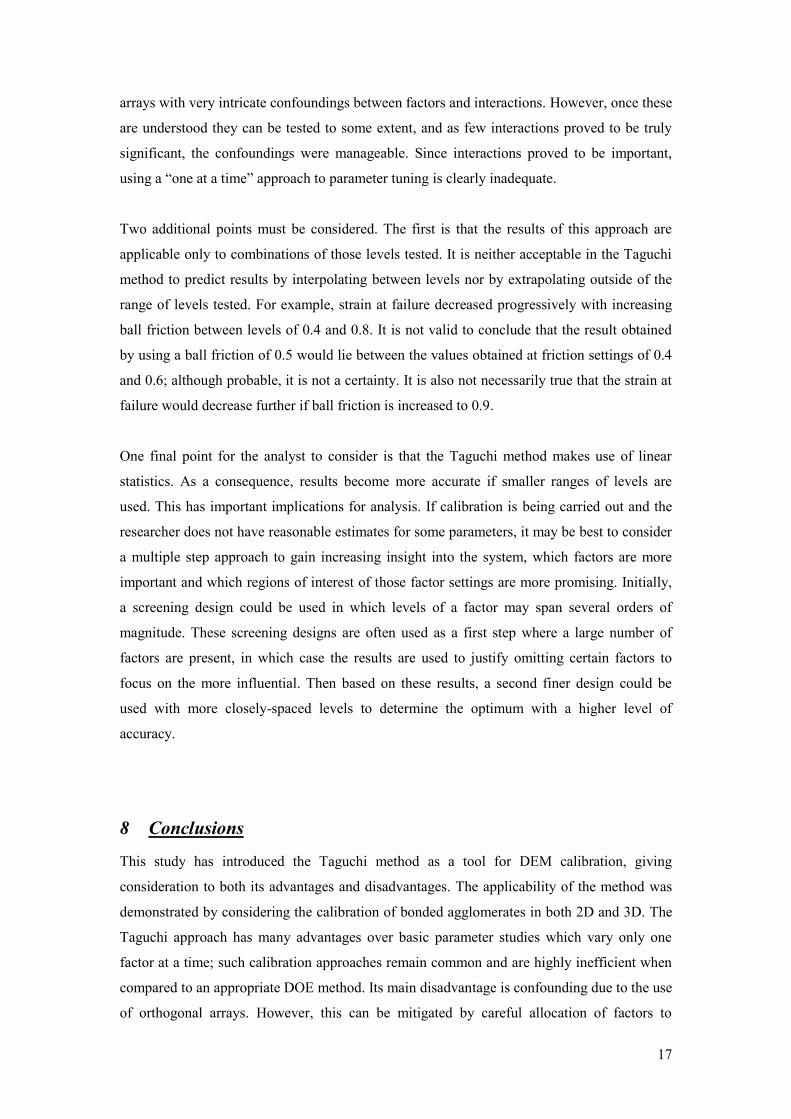
3.3 Particle Crushing Conditions

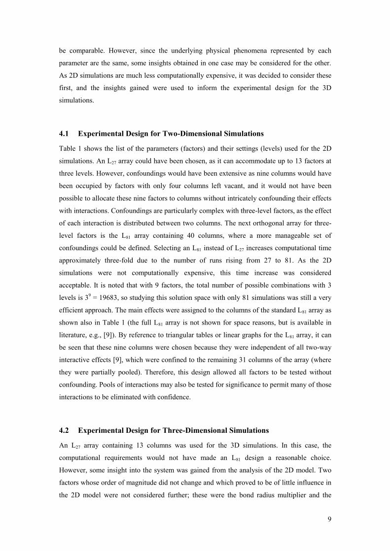
To simulate a particle crushing test, each agglomerate was subject to uniaxial compression

between stiff, horizontal, frictionless platens, as shown in Fig. 1 (similar to [14,19]). This

compression was strain-controlled, and all agglomerates were compressed to a strain of 20%.

In both the two- and three-dimensional cases, the bottom platen remained at rest and the

upper platen moved towards it at 10 mm/s. This velocity was sufficiently low to ensure that

forces on the top and bottom platens were equivalent during crushing, i.e., quasi-static loading

was attained. The initial distance between the platens was equal to the agglomerate height.

8

3.4 Agglomerate Bonds and Contact Models

The inter-sphere contacts were modelled using a standard linear contact model, with linear

springs in the contact normal and tangential directions. Spring normal and shear stiffnesses

were calculated from stiffnesses of the contacting bodies [18]. Parallel bonds were used to

cement the disks or spheres together to form a bonded agglomerate. These may be envisioned

as a set of elastic springs with constant normal and shear stiffnesses, uniformly distributed

over a cross-section lying on the contact plane and centred on the contact point; further details

are given by [20]. When simulating particles made of aggregates of powder grains glued

together with a finite volume of cement, the parallel bonds have an advantage over simple

contact bonds as the parallel bonds transmit both force and moment (bending and twisting in

3D; bending only in 2D), whereas contact bonds are restricted to the transmission of force

only. Parallel bonds require the specification of five parameter values in PFC2D/3D: normal

and shear strengths, normal and shear stiffnesses and bond radius. These spring stiffnesses

cause a force and moment to be developed if the bonded particles move relative to one

another. The maximum normal and shear stresses acting at the periphery of the parallel bond

are calculated from beam theory and compared to the corresponding bond strengths. If the

maximum normal tensile stress is greater than the bond normal strength, the parallel bond is

deemed to have failed and is deleted from the model. The same occurs if the maximum shear

stress exceeds the bond shear strength. Bond radius is set by specifying the parameter in

the software; the bond radius is the product of and the radius of the smaller of the two

particles interacting in the bond (equivalent to the radius of the circular region containing

springs in 3D). must be positive; if it is equal to 1, the bond radius is the same as the

radius of the smaller particle in the bond. Once a bond breaks, or if a new contact is formed

after the cementing stage of the simulation, the contact interaction between two particles is

frictional.

4 Experimental Designs

The 2D and 3D models needed to be assessed independently because although many

parameters were the same, the range of values of certain parameters which gave a feasible

response differed by orders of magnitude in many cases. This can be attributed to the

kinematic constraints imposed in 2D compared to the 3D case; in 2D, each base particle has

three, rather than six, degrees of freedom and particle motion is restricted to a single plane. In

ANOVA, whether a factor or interaction is important or negligible is a comparative result

which depends on the range of values tested. This implies that the 2D and 3D results may not

9

be comparable. However, since the underlying physical phenomena represented by each

parameter are the same, some insights obtained in one case may be considered for the other.

As 2D simulations are much less computationally expensive, it was decided to consider these

first, and the insights gained were used to inform the experimental design for the 3D

simulations.

4.1 Experimental Design for Two-Dimensional Simulations

Table 1 shows the list of the parameters (factors) and their settings (levels) used for the 2D

simulations. An L27 array could have been chosen, as it can accommodate up to 13 factors at

three levels. However, confoundings would have been extensive as nine columns would have

been occupied by factors with only four columns left vacant, and it would not have been

possible to allocate these nine factors to columns without intricately confounding their effects

with interactions. Confoundings are particularly complex with three-level factors, as the effect

of each interaction is distributed between two columns. The next orthogonal array for three-

level factors is the L81 array containing 40 columns, where a more manageable set of

confoundings could be defined. Selecting an L81 instead of L27 increases computational time

approximately three-fold due to the number of runs rising from 27 to 81. As the 2D

simulations were not computationally expensive, this time increase was considered

acceptable. It is noted that with 9 factors, the total number of possible combinations with 3

levels is 39 = 19683, so studying this solution space with only 81 simulations was still a very

efficient approach. The main effects were assigned to the columns of the standard L81 array as

shown also in Table 1 (the full L81 array is not shown for space reasons, but is available in

literature, e.g., [9]). By reference to triangular tables or linear graphs for the L81 array, it can

be seen that these nine columns were chosen because they were independent of all two-way

interactive effects [9], which were confined to the remaining 31 columns of the array (where

they were partially pooled). Therefore, this design allowed all factors to be tested without

confounding. Pools of interactions may also be tested for significance to permit many of those

interactions to be eliminated with confidence.

4.2 Experimental Design for Three-Dimensional Simulations

An L27 array containing 13 columns was used for the 3D simulations. In this case, the

computational requirements would not have made an L81 design a reasonable choice.

However, some insight into the system was gained from the analysis of the 2D model. Two

factors whose order of magnitude did not change and which proved to be of little influence in

the 2D model were not considered further; these were the bond radius multiplier and the

10

random number seed. Their values were set at the median values in Table 1. One additional

factor that needed to be included was the percentage of balls deleted from the lattice. The

number of degrees of freedom remaining allowed only two interactive effects to be

considered. Thus, the design was developed assuming that all but two interactive effects could

be neglected, and factors were allocated to columns to allow these two chosen interactions to

be assessed. This was deemed to be appropriate on the basis of the 2D analysis, and the

interactive effects selected for consideration were bond shear strength and bond shear

stiffness, and bond shear strength and ball shear stiffness.

Table 2 shows the factors and levels used for the 3D simulations, along with the columns of

the standard L27 array assigned to each factor. The interaction between bond shear strength

and stiffness (interaction I) was contained in columns 3 and 4, and that between bond shear

strength and ball shear stiffness in columns 6 and 7 (interaction II). The remaining

interactions were intricately confounded with factors, and were all assumed to be negligible in

the data analysis.

5 Simulation Responses

The objective of the study was to achieve a controlled mechanical response for the

agglomerate as a whole. The mechanics of an agglomerate response under uniaxial

compression are often complex and highly non-linear. The force-deflection behaviour may

include multiple local maxima, and alternating periods of strain softening and strain

hardening. As discussed by Cavarretta [21], the load deformation response is affected by

asperity failure, particle rotation, elastic and plastic response of the solid particle material and

gross fragmentation. Therefore, one single response is insufficient to characterise the

compression mechanics and in this study, four responses were selected:

1. The normal force on the platens at 10% strain (N)

2. The normal force at the point of failure of the agglomerate (N)

3. The strain at the point of failure of the agglomerate (-)

4. The agglomerate stiffness (N m-1

)

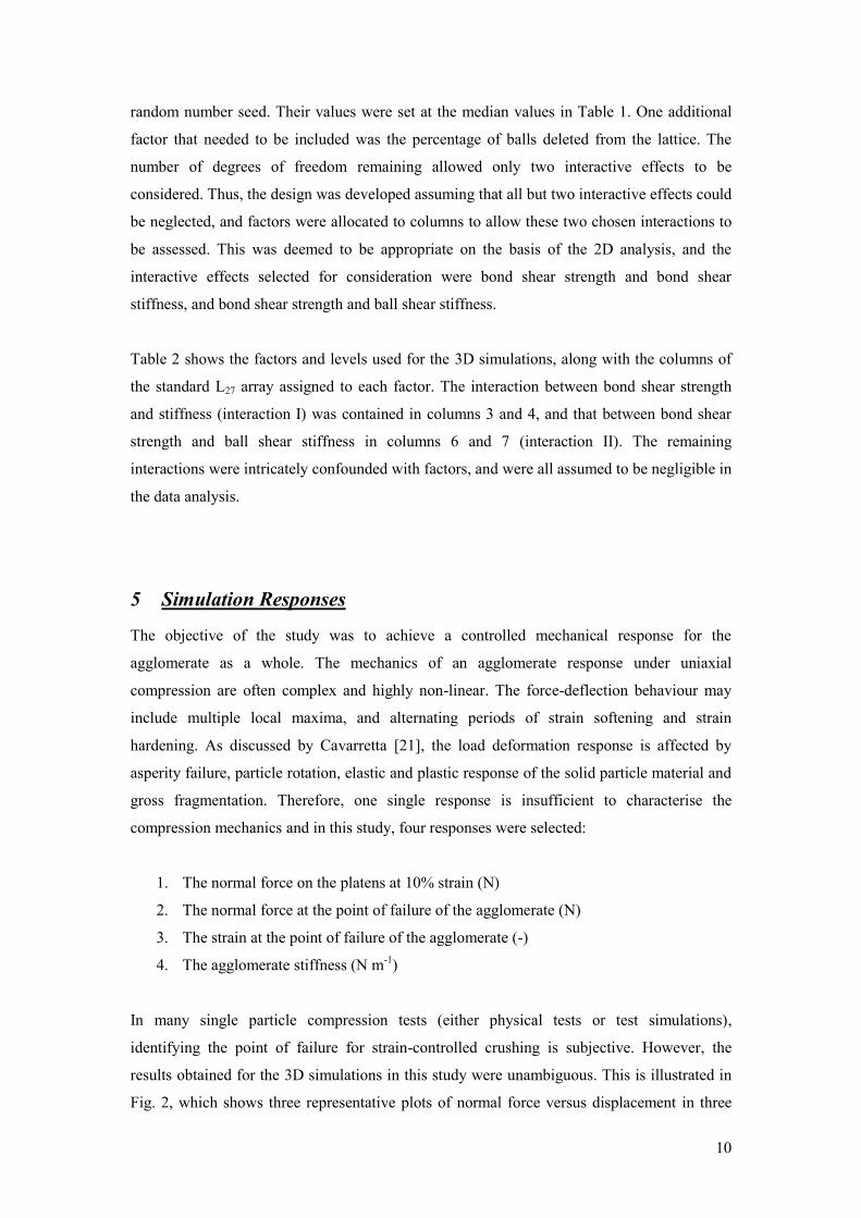
In many single particle compression tests (either physical tests or test simulations),

identifying the point of failure for strain-controlled crushing is subjective. However, the

results obtained for the 3D simulations in this study were unambiguous. This is illustrated in

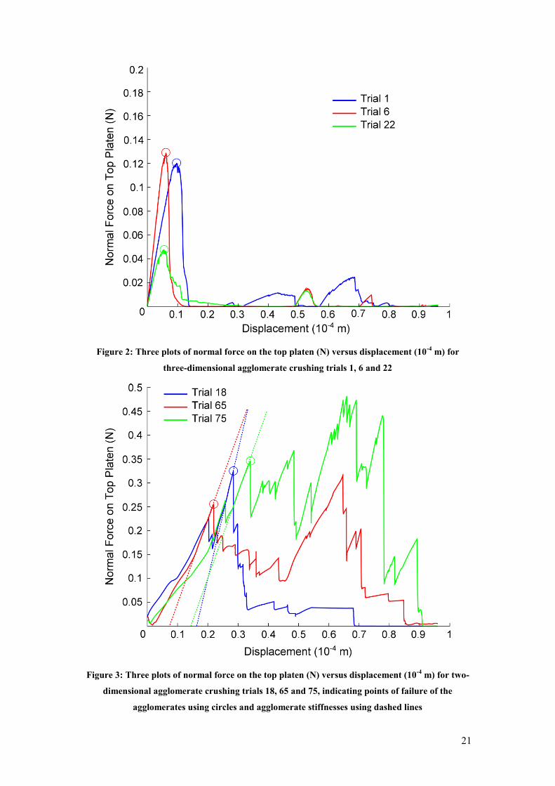
Fig. 2, which shows three representative plots of normal force versus displacement in three

11

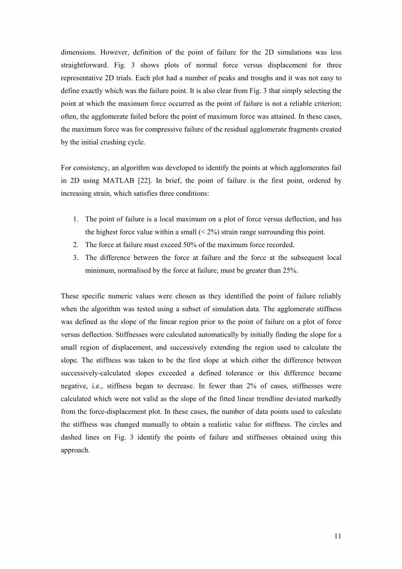
dimensions. However, definition of the point of failure for the 2D simulations was less

straightforward. Fig. 3 shows plots of normal force versus displacement for three

representative 2D trials. Each plot had a number of peaks and troughs and it was not easy to

define exactly which was the failure point. It is also clear from Fig. 3 that simply selecting the

point at which the maximum force occurred as the point of failure is not a reliable criterion;

often, the agglomerate failed before the point of maximum force was attained. In these cases,

the maximum force was for compressive failure of the residual agglomerate fragments created

by the initial crushing cycle.

For consistency, an algorithm was developed to identify the points at which agglomerates fail

in 2D using MATLAB [22]. In brief, the point of failure is the first point, ordered by

increasing strain, which satisfies three conditions:

1. The point of failure is a local maximum on a plot of force versus deflection, and has

the highest force value within a small (< 2%) strain range surrounding this point.

2. The force at failure must exceed 50% of the maximum force recorded.

3. The difference between the force at failure and the force at the subsequent local

minimum, normalised by the force at failure, must be greater than 25%.

These specific numeric values were chosen as they identified the point of failure reliably

when the algorithm was tested using a subset of simulation data. The agglomerate stiffness

was defined as the slope of the linear region prior to the point of failure on a plot of force

versus deflection. Stiffnesses were calculated automatically by initially finding the slope for a

small region of displacement, and successively extending the region used to calculate the

slope. The stiffness was taken to be the first slope at which either the difference between

successively-calculated slopes exceeded a defined tolerance or this difference became

negative, i.e., stiffness began to decrease. In fewer than 2% of cases, stiffnesses were

calculated which were not valid as the slope of the fitted linear trendline deviated markedly

from the force-displacement plot. In these cases, the number of data points used to calculate

the stiffness was changed manually to obtain a realistic value for stiffness. The circles and

dashed lines on Fig. 3 identify the points of failure and stiffnesses obtained using this

approach.

12

6 Analytical Procedure

The data were analysed using STATISTICA [23]. Firstly, an ANOVA was applied to the raw

data obtained for the 2D simulations for each of the four response parameters. Marginal

means were calculated and presented graphically; these show the average effect of choosing a

particular factor level compared to the global average. In the Taguchi method, estimates for

any combination of settings are calculated by addition of the respective marginal means,

which implies assuming that all interactions are negligible. In some cases, it is possible to

correct for interactions (when the effect of that interaction is confounded neither with any

factor nor with other potentially significant interactions). In order to test the predictive ability

of this procedure, a validation set was subsequently run by choosing 10 random combinations

of levels (other than the 81 already used), and the responses obtained by running DEM

simulations using these randomly-chosen levels were compared to those predicted by the

marginal means addition.

There were 9 factors in the design and therefore 36 possible two-way interactions. As

interactions of three-level factors are distributed between two columns, most of the columns

of the L81 which were not occupied by factors contained parts of multiple interactions, e.g.,

column 3 contained parts of the interactions between bond radius multiplier and bond normal

strength, bond normal stiffness and bond shear stiffness and ball shear stiffness and random

number seed. In order to evaluate the potential significance of the interactions, each was

assessed in turn, assuming all others to be negligible. If the added effect of considering an

interaction in this test was negligible, then the interaction could be neglected. Otherwise, it

could potentially be important, but this was not certain as the effect was confounded with

other interactions.

In the 3D analysis, all but two interactions were assumed to be negligible. Estimates of the

response were corrected for these two interactive effects, and they were also tested for

statistical significance and compared with effects of factors.

7 Results and Discussion

7.1 Two-Dimensional Results

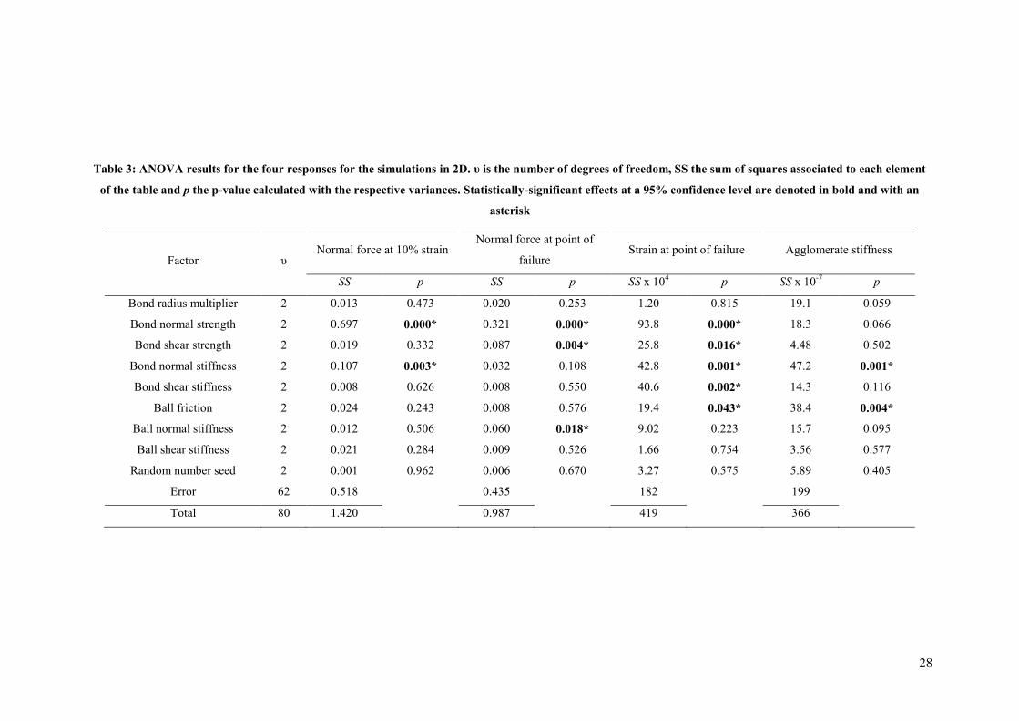
The ANOVA results are shown in Table 3. The statistical significance was assessed with the

p-value: effects were deemed to be significant at the 90%, 95% or 99% significance levels if

13

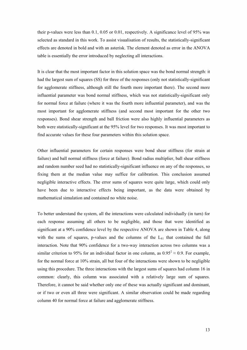
their p-values were less than 0.1, 0.05 or 0.01, respectively. A significance level of 95% was

selected as standard in this work. To assist visualisation of results, the statistically-significant

effects are denoted in bold and with an asterisk. The element denoted as error in the ANOVA

table is essentially the error introduced by neglecting all interactions.

It is clear that the most important factor in this solution space was the bond normal strength: it

had the largest sum of squares (SS) for three of the responses (only not statistically-significant

for agglomerate stiffness, although still the fourth more important there). The second more

influential parameter was bond normal stiffness, which was not statistically-significant only

for normal force at failure (where it was the fourth more influential parameter), and was the

most important for agglomerate stiffness (and second most important for the other two

responses). Bond shear strength and ball friction were also highly influential parameters as

both were statistically-significant at the 95% level for two responses. It was most important to

find accurate values for these four parameters within this solution space.

Other influential parameters for certain responses were bond shear stiffness (for strain at

failure) and ball normal stiffness (force at failure). Bond radius multiplier, ball shear stiffness

and random number seed had no statistically-significant influence on any of the responses, so

fixing them at the median value may suffice for calibration. This conclusion assumed

negligible interactive effects. The error sums of squares were quite large, which could only

have been due to interactive effects being important, as the data were obtained by

mathematical simulation and contained no white noise.

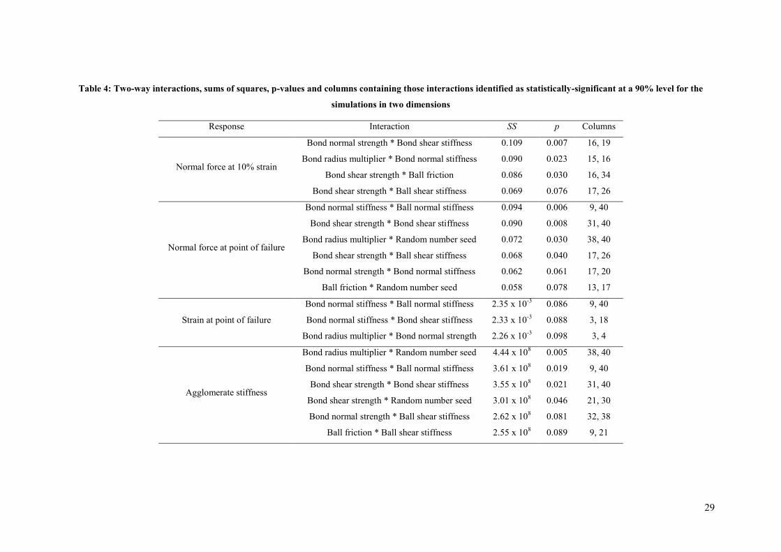
To better understand the system, all the interactions were calculated individually (in turn) for

each response assuming all others to be negligible, and those that were identified as

significant at a 90% confidence level by the respective ANOVA are shown in Table 4, along

with the sums of squares, p-values and the columns of the L81 that contained the full

interaction. Note that 90% confidence for a two-way interaction across two columns was a

similar criterion to 95% for an individual factor in one column, as 0.952 ≈ 0.9. For example,

for the normal force at 10% strain, all but four of the interactions were shown to be negligible

using this procedure. The three interactions with the largest sums of squares had column 16 in

common: clearly, this column was associated with a relatively large sum of squares.

Therefore, it cannot be said whether only one of these was actually significant and dominant,

or if two or even all three were significant. A similar observation could be made regarding

column 40 for normal force at failure and agglomerate stiffness.

14

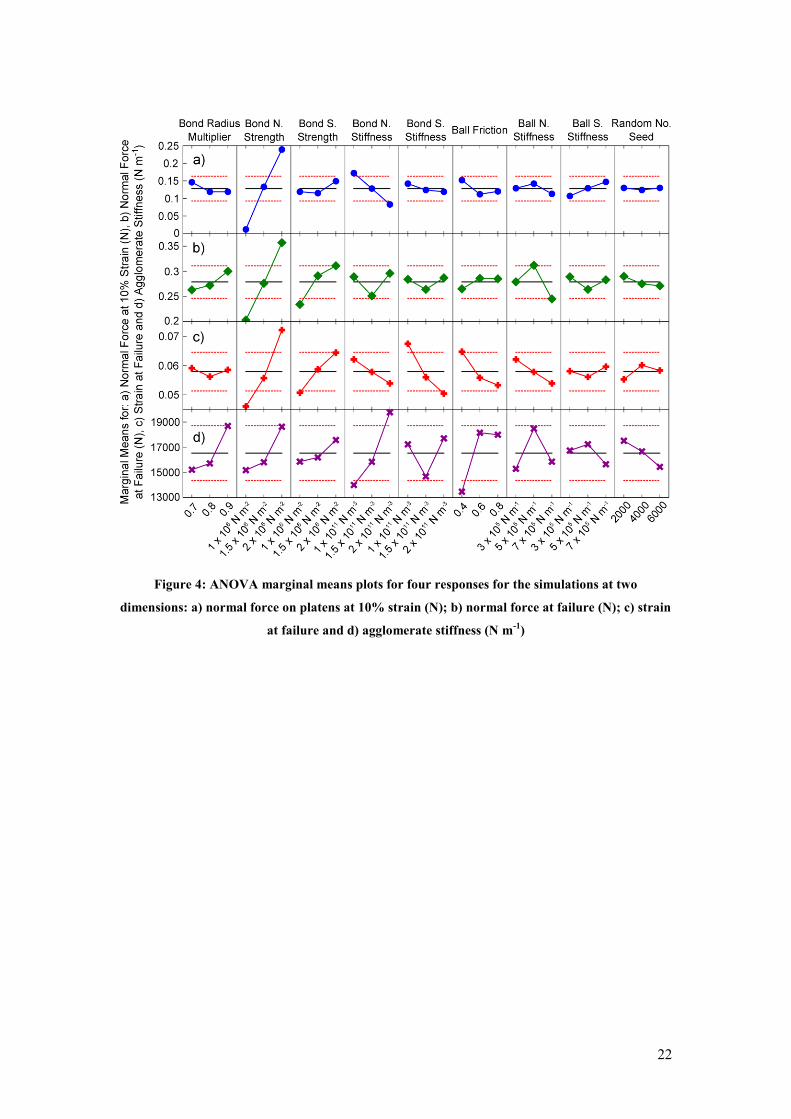
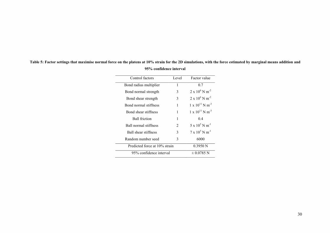
Fig. 4 shows the stacked marginal means plots of the data, where the horizontal dashed limits

denote ± two standard errors. For those factors identified as significant in Table 3, it is clear

that increasing the normal strength of the parallel bonds tended to increase the normal force at

10% strain, while increasing their normal stiffness had the opposite effect. These observations

make sense from a mechanical point of view. If the analyst seeks to maximise this force to

give stronger agglomerates, this could be achieved by choosing the settings shown in Table 5.

The response estimated by simple addition of the marginal means (i.e., neglecting all

interactive effects) was 0.395 ± 0.0785 N. The force at failure increased if higher values of

parallel bond normal and shear strength were used, while using an intermediate ball normal

stiffness of 5 x 105 N m

-1 increased this response, i.e., on average, selecting these settings

increased the force at which the agglomerate failed under uniaxial compression. The strain at

failure may be maximised by choosing high settings for bond normal and shear strength and

the lowest settings for ball friction and both bond stiffnesses, within the range tested. The

settings for maximisation of agglomerate stiffness were similar: a high value for bond normal

stiffness and the intermediate setting for ball friction of 0.6, although there was little

difference between the intermediate and high settings of this factor.

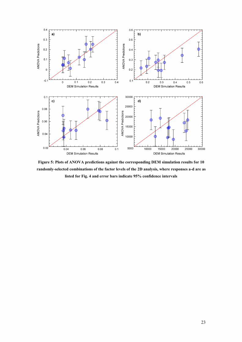
To assess the predictive ability of the marginal means addition (i.e., the inaccuracy resulting

from neglecting all interactions in the estimation of a specific response), 10 combinations of

factor levels, each different to the 81 combinations already used in the design, were selected

at random. For each combination, the responses (normal force at 10% strain, normal force at

failure, strain at failure and agglomerate stiffness) were found in two ways:

1. By experiment, running a DEM simulation using the appropriate combination of

factor levels and obtaining the data as was done for the initial 81 trials.

2. By adding the marginal means for the respective factor settings to the global average

for each response.

Fig. 5 compares the estimates of the marginal means additions with the simulation results.

Results were mixed, with certain responses performing better than others. This is not

surprising, as neglecting the interactive effects was a major source of error, as Table 3 shows.

For the normal force at failure considered in Fig. 5b, the marginal means estimates over-

predicted forces which had very small values, but under-predicted larger forces. A tendency

to under-estimate agglomerate stiffness (Fig. 5d) was also apparent for eight of the

combinations tested. It is evident that neglecting all interactive effects would be very limiting.

Therefore, the most basic application of the Taguchi method provided some inconclusive

results at this stage. It would be necessary to untangle some of the interactions to assess them

15

properly and then apply the Taguchi optimisation procedure for parameter calibration with the

appropriate corrections. This suggests that a two-step procedure may be a better option than

larger designs. A two-level design could be used first to eliminate (pools of) interactions that

are not significant and then a three-level design may be better defined, even though it may

now require fewer runs. While a two-way interaction with two or three levels in the factors

are not the same, the reality of most systems is that two levels are often sufficient to reveal the

nature of the most common interactions. It is not common that an interaction may prove to be

negligible with a two-level design and show relevance with a three-level design.

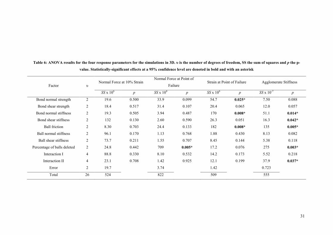
7.2 Three-Dimensional Results

The same four overall responses were analysed in 3D, i.e., normal force at 10% strain, normal

force at failure, strain at failure and agglomerate stiffness. As the 2D results indicated not

only many interactions that could be neglected, but also the two factors of least significance, a

second design with reduced data requirements could be established (using an L27 array). The

ANOVA results, which include two interactions that could be assessed fully and

independently (once the others had been assumed negligible), are shown in Table 6.

The results in 3D were comparable to those in 2D, even though different ranges were used for

many parameters. However, the most significant parameters were not always the same as in

2D. This is not surprising since an analysis of this type is always relative to the ranges of

values used, i.e., to the solution space being scanned. It is also noted that the inclusion of two

interactions (each requiring four degrees of freedom) and the more limited number of data

naturally resulted in a much larger confidence interval. Therefore, this design did not identify

the limit of statistical significance as clearly as the L81. Considering the normal force on the

platens at 10% strain, no factor was now statistically-significant in 3D. As this was partially

attributable to the low number of degrees of freedom of the error, it was more appropriate to

analyse the relative importance of the factors and interactions using their sums of squares.

The percentage of balls deleted was the overwhelming influence on force at failure. The three

factors that significantly affected the strain at failure were three of the five which were

identified as significant in 2D. The percentage of balls deleted significantly influenced the

agglomerate stiffness, in addition to ball friction and both bond stiffnesses; both bond normal

stiffness and ball friction were also significant in 2D. Interaction II, between bond shear

strength and ball shear stiffness, was significant at the 95% level for the agglomerate stiffness

response. This is particularly interesting since neither factor in the interaction was one of

those four identified as significant independently, so the interaction was clearly very

important.

16

It is noted that the relative magnitude of the error was much smaller than in 2D. This could

also be quantified by the coefficient of determination (R2), which is the percentage of the

variance of the data explained by the factors and interactions. For the four responses in Table

6, R2 values were 98.1%, 99.8%, 99.9% and 99.9%, respectively. When coefficients of

determination were calculated without including both interactions, the results were reduced to

86.5%, 99.2%, 97.2% and 95.9%, respectively. This result confirmed the importance of

considering these two interactions.

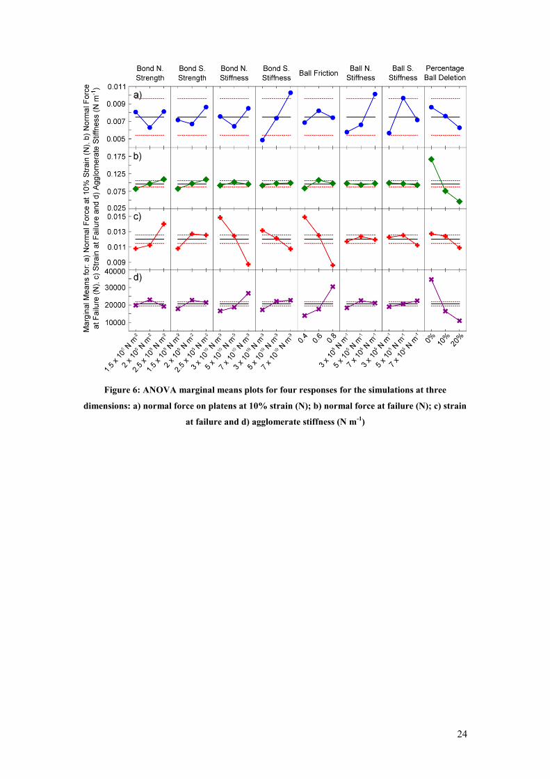
The stacked marginal means plots are shown for the main effects in Fig. 6. Force at failure

was increased by using 0% ball deletion. The settings to maximise strain at failure were

identical to those in 2D for the three factors identified as significant. High bond normal and

shear stiffnesses and ball friction and low percentage ball deletion maximised agglomerate

stiffness. However, this analysis with marginal means alone was no longer complete, as the

correction for interactive effects also needed to be taken into consideration.

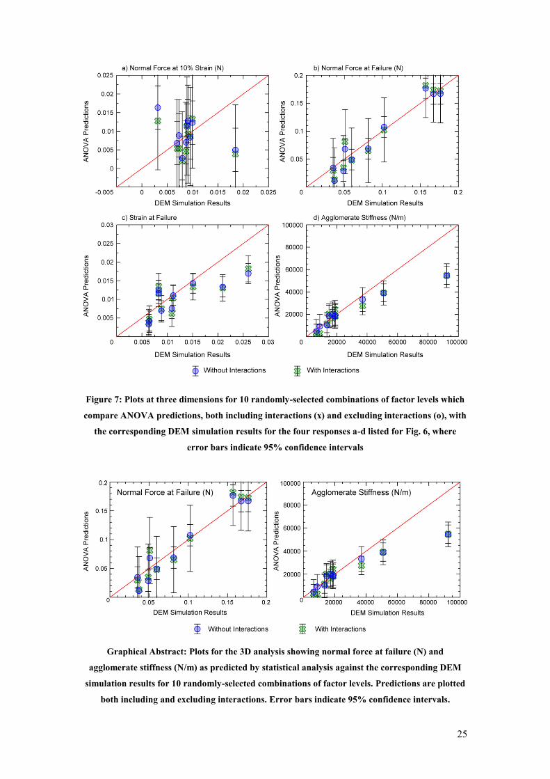
The predictive ability of marginal means addition was again tested by comparing the results

thus estimated with actual simulation results performed for 10 random combinations of

settings (other than the 27 already performed). Results are shown in Fig. 7, both considering

and omitting the interactive effects.

Both sets of predictions were very close, and the increase in accuracy obtained by correcting

for the interactive effects was quantitatively small. The predictions in 3D were considerably

more accurate than those in 2D, with a lower number of anomalous predictions. Predictions

were particularly accurate for all normal force at failure points tested (Fig. 7b) and for low

agglomerate stiffnesses (Fig. 7d). The predictions of normal force at 10% strain were least

accurate. The better predictive ability in 3D, in comparison with the 2D case, was due to the

smaller proportion of the total sums of squares in the ANOVA table attributed to unexplained

variance (error).

7.3 Discussion

The results in Sections 7.1 and 7.2 demonstrate that the application of the Taguchi method is

appropriate for DEM calibrations using bonded agglomerates. Good predictive ability was

demonstrated when interactions were considered. It is clear that accounting for interactive

effects is important; therefore, a two (or more) step approach is preferable to a single (larger)

design. This could be a problem with the Taguchi method because it relies on orthogonal

17

arrays with very intricate confoundings between factors and interactions. However, once these

are understood they can be tested to some extent, and as few interactions proved to be truly

significant, the confoundings were manageable. Since interactions proved to be important,

using a “one at a time” approach to parameter tuning is clearly inadequate.

Two additional points must be considered. The first is that the results of this approach are

applicable only to combinations of those levels tested. It is neither acceptable in the Taguchi

method to predict results by interpolating between levels nor by extrapolating outside of the

range of levels tested. For example, strain at failure decreased progressively with increasing

ball friction between levels of 0.4 and 0.8. It is not valid to conclude that the result obtained

by using a ball friction of 0.5 would lie between the values obtained at friction settings of 0.4

and 0.6; although probable, it is not a certainty. It is also not necessarily true that the strain at

failure would decrease further if ball friction is increased to 0.9.

One final point for the analyst to consider is that the Taguchi method makes use of linear

statistics. As a consequence, results become more accurate if smaller ranges of levels are

used. This has important implications for analysis. If calibration is being carried out and the

researcher does not have reasonable estimates for some parameters, it may be best to consider

a multiple step approach to gain increasing insight into the system, which factors are more

important and which regions of interest of those factor settings are more promising. Initially,

a screening design could be used in which levels of a factor may span several orders of

magnitude. These screening designs are often used as a first step where a large number of

factors are present, in which case the results are used to justify omitting certain factors to

focus on the more influential. Then based on these results, a second finer design could be

used with more closely-spaced levels to determine the optimum with a higher level of

accuracy.

8 Conclusions

This study has introduced the Taguchi method as a tool for DEM calibration, giving

consideration to both its advantages and disadvantages. The applicability of the method was

demonstrated by considering the calibration of bonded agglomerates in both 2D and 3D. The

Taguchi approach has many advantages over basic parameter studies which vary only one

factor at a time; such calibration approaches remain common and are highly inefficient when

compared to an appropriate DOE method. Its main disadvantage is confounding due to the use

of orthogonal arrays. However, this can be mitigated by careful allocation of factors to

18

columns of the array to permit the testing of selected interactions, and also by using multiple

smaller experimental designs rather than one large design.

The Taguchi method is certainly suitable for DEM calibration of bonded agglomerates,

although it is important to identify and include key interactive effects in the analysis to ensure

good predictive ability. Close correspondence was obtained between ANOVA predictions of

the measured responses and the DEM simulation results in 3D, with all R2 values exceeding

98%. For the 2D simulations, predictions were made using solely main effects, although some

interactions were statistically-significant. As expected, these predictions were considerably

poorer than those made in 3D since all interactions were disregarded.

For both two- and three-dimensional simulations, parallel bond normal strength, bond normal

stiffness and ball friction all had a statistically-significant effect on strain at failure at a 95%

level. Bond normal stiffness and ball friction had a significant effect on agglomerate stiffness.

By increasing parallel bond normal stiffness, the agglomerate stiffness was increased and the

strain at failure was decreased. Strain at failure may be maximised by choosing a high bond

normal strength and low values of ball friction and bond normal stiffness.

9 Acknowledgements

Kevin Hanley would like to acknowledge financial support from the Irish Research Council

for Science, Engineering and Technology (IRCSET).

10 References

[1] P.A. Cundall, A discontinuous future for numerical modelling in geomechanics?, Geotech.

Eng. 149(1) (2001) 41–47.

[2] P.A. Cundall, O.D.L. Strack, A discrete numerical model for granular assemblies,

Géotechnique 29(1) (1979) 47–65.

[3] Z. Asaf, D. Rubinstein, I. Shmulevich, Evaluation of link-track performances using DEM,

J. Terramechanics 43(2) (2006) 141–161.

[4] C.J. Coetzee, D.N.J. Els, Calibration of discrete element parameters and the modelling of

silo discharge and bucket filling, Comput. Electron. Agr. 65(2) (2009) 198–212.

19

[5] M. Doležalová, P. Czene, F. Havel, Micromechanical modeling of stress path effects using

PFC2D code, in: H. Konietzky (Ed.), Numerical Modeling in Micromechanics via Particle

Methods, Balkema, Lisse, 2002, pp. 173–182.

[6] J. Yoon, Application of experimental design and optimization to PFC model calibration in

uniaxial compression simulation, Int. J. Rock Mech. Min. 44(6) (2007) 871–889.

[7] J. Favier, D. Curry, R. LaRoche, Calibration of DEM material models to approximate bulk

particle characteristics, 6th World Congress on Particle Technology, Nuremberg, Germany,

2010.

[8] M. Johnstone, J. Ooi, Calibration of DEM models using rotating drum and confined

compression measurements, 6th World Congress on Particle Technology, Nuremberg,

Germany, 2010.

[9] G. Taguchi, System of experimental design, UNIPUB/Kraus International Publications,

New York, 1987.

[10] P.J. Ross, Taguchi techniques for quality engineering: loss function, orthogonal

experiments, parameter and tolerance design, McGraw-Hill, New York, 1988.

[11] G.E.P. Box, S. Bisgaard, C.A. Fung, An explanation and critique of Taguchi’s

contributions to quality engineering, Qual. Reliab. Eng. Int. 4(2) (1988) 123–131.

[12] D.C. Montgomery, Design and Analysis of Experiments [International Student Version],

John Wiley & Sons, New York, 2009.

[13] C. Thornton, L. Liu, How do agglomerates break?, Powder Technol. 143–144 (2004)

110–116.

[14] Y.P. Cheng, Y. Nakata, M.D. Bolton, Discrete element simulation of crushable soil,

Géotechnique 53(7) (2003) 633–641.

[15] G.R. McDowell, O. Harireche, Discrete element modelling of yielding and normal

compression of sand, Géotechnique 52(4) (2002) 299–304.

[16] M. Lu, G. McDowell, Discrete element modelling of railway ballast under monotonic

and cyclic triaxial loading, Géotechnique 60(6) (2010) 459–467.

[17] Itasca Consulting Group, PFC2D: Particle Flow Code in Two Dimensions, Minneapolis,

Minnesota, 2008.

[18] Itasca Consulting Group, PFC3D: Particle Flow Code in Three Dimensions,

Minneapolis, Minnesota, 2008.

[19] C. Thornton, M.T. Ciomocos, M.J. Adams, Numerical simulations of diametrical

compression tests on agglomerates, Powder Technol. 140(3) (2004) 258–267.

[20] D.O. Potyondy, P.A. Cundall, A bonded-particle model for rock, Int. J. Rock Mech. Min.

41(8) (2004) 1329–1364.

[21] I. Cavarretta, The Influence of Particle Characteristics on the Engineering Behaviour of

Granular Materials, PhD Thesis, Imperial College London, 2009.

20

[22] The MathWorks, MATLAB, v.7.0.1 [R14SP1], Natick, MA, USA, 2001.

[23] StatSoft, Inc., STATISTICA, v.7.1, Tulsa, OK, USA, 2005.

11 Figures

Figure 1: Illustration of uniaxial agglomerate crushing between two stiff horizontal platens for

the 3D simulations

21

Figure 2: Three plots of normal force on the top platen (N) versus displacement (10-4

m) for

three-dimensional agglomerate crushing trials 1, 6 and 22

Figure 3: Three plots of normal force on the top platen (N) versus displacement (10-4

m) for two-

dimensional agglomerate crushing trials 18, 65 and 75, indicating points of failure of the

agglomerates using circles and agglomerate stiffnesses using dashed lines

22

Figure 4: ANOVA marginal means plots for four responses for the simulations at two

dimensions: a) normal force on platens at 10% strain (N); b) normal force at failure (N); c) strain

at failure and d) agglomerate stiffness (N m-1

)

23

Figure 5: Plots of ANOVA predictions against the corresponding DEM simulation results for 10

randomly-selected combinations of the factor levels of the 2D analysis, where responses a-d are as

listed for Fig. 4 and error bars indicate 95% confidence intervals

24

Figure 6: ANOVA marginal means plots for four responses for the simulations at three

dimensions: a) normal force on platens at 10% strain (N); b) normal force at failure (N); c) strain

at failure and d) agglomerate stiffness (N m-1

)

25

Figure 7: Plots at three dimensions for 10 randomly-selected combinations of factor levels which

compare ANOVA predictions, both including interactions (x) and excluding interactions (o), with

the corresponding DEM simulation results for the four responses a-d listed for Fig. 6, where

error bars indicate 95% confidence intervals

Graphical Abstract: Plots for the 3D analysis showing normal force at failure (N) and

agglomerate stiffness (N/m) as predicted by statistical analysis against the corresponding DEM

simulation results for 10 randomly-selected combinations of factor levels. Predictions are plotted

both including and excluding interactions. Error bars indicate 95% confidence intervals.

26

12 Tables

Table 1: Factors varied, levels used and column of the standard L81 array assigned to each factor for simulations at two dimensions

Control factors Levels Column

assigned 1 2 3

Bond radius multiplier (-) 0.7 0.8 0.9 1

Bond normal strength (N m-2

) 1 x 106 1.5 x 10

6 2 x 10

6 2

Bond shear strength (N m-2

) 1 x 106 1.5 x 10

6 2 x 10

6 5

Bond normal stiffnessa (N m

-3) 1 x 10

11 1.5 x 10

11 2 x 10

11 14

Bond shear stiffnessa (N m

-3) 1 x 10

11 1.5 x 10

11 2 x 10

11 22

Ball friction (-) 0.4 0.6 0.8 25

Ball normal stiffnessb (N m

-1) 3 x 10

5 5 x 10

5 7 x 10

5 27

Ball shear stiffnessb (N m

-1) 3 x 10

5 5 x 10

5 7 x 10

5 35

Random number seed (-) 2000 4000 6000 39

a Stiffness as [stress/displacement]

b Stiffness as [force/displacement]

27

Table 2: Factors varied, levels used and column of the standard L27 array assigned to each factor for simulations at three dimensions

Control factors Levels Column

assigned 1 2 3

Bond shear strength (N m-2

) 1.5 x 105

2 x 105

2.5 x 105

1

Bond shear stiffness (N m-3

) 3 x 1010

5 x 1010

7 x 1010

2

Ball shear stiffness (N m-1

) 3 x 105

5 x 105

7 x 105

5

Bond normal strength (N m-2

) 1.5 x 105

2 x 105

2.5 x 105

8

Ball friction (-) 0.4 0.6 0.8 9

Percentage of balls deleted (%) 0 10 20 10

Bond normal stiffness (N m-3

) 3 x 1010

5 x 1010

7 x 1010

11

Ball normal stiffness (N m-1

) 3 x 105

5 x 105

7 x 105

12

28

Table 3: ANOVA results for the four responses for the simulations in 2D. υ is the number of degrees of freedom, SS the sum of squares associated to each element

of the table and p the p-value calculated with the respective variances. Statistically-significant effects at a 95% confidence level are denoted in bold and with an

asterisk

Factor υ Normal force at 10% strain

Normal force at point of

failure Strain at point of failure Agglomerate stiffness

SS p SS p SS x 104 p SS x 10

-7 p

Bond radius multiplier 2 0.013 0.473 0.020 0.253 1.20 0.815 19.1 0.059

Bond normal strength 2 0.697 0.000* 0.321 0.000* 93.8 0.000* 18.3 0.066

Bond shear strength 2 0.019 0.332 0.087 0.004* 25.8 0.016* 4.48 0.502

Bond normal stiffness 2 0.107 0.003* 0.032 0.108 42.8 0.001* 47.2 0.001*

Bond shear stiffness 2 0.008 0.626 0.008 0.550 40.6 0.002* 14.3 0.116

Ball friction 2 0.024 0.243 0.008 0.576 19.4 0.043* 38.4 0.004*

Ball normal stiffness 2 0.012 0.506 0.060 0.018* 9.02 0.223 15.7 0.095

Ball shear stiffness 2 0.021 0.284 0.009 0.526 1.66 0.754 3.56 0.577

Random number seed 2 0.001 0.962 0.006 0.670 3.27 0.575 5.89 0.405

Error 62 0.518 0.435 182 199

Total 80 1.420 0.987 419 366

29

Table 4: Two-way interactions, sums of squares, p-values and columns containing those interactions identified as statistically-significant at a 90% level for the

simulations in two dimensions

Response Interaction SS p Columns

Normal force at 10% strain

Bond normal strength * Bond shear stiffness 0.109 0.007 16, 19

Bond radius multiplier * Bond normal stiffness 0.090 0.023 15, 16

Bond shear strength * Ball friction 0.086 0.030 16, 34

Bond shear strength * Ball shear stiffness 0.069 0.076 17, 26

Normal force at point of failure

Bond normal stiffness * Ball normal stiffness 0.094 0.006 9, 40

Bond shear strength * Bond shear stiffness 0.090 0.008 31, 40

Bond radius multiplier * Random number seed 0.072 0.030 38, 40

Bond shear strength * Ball shear stiffness 0.068 0.040 17, 26

Bond normal strength * Bond normal stiffness 0.062 0.061 17, 20

Ball friction * Random number seed 0.058 0.078 13, 17

Strain at point of failure

Bond normal stiffness * Ball normal stiffness 2.35 x 10-3

0.086 9, 40

Bond normal stiffness * Bond shear stiffness 2.33 x 10-3

0.088 3, 18

Bond radius multiplier * Bond normal strength 2.26 x 10-3

0.098 3, 4

Agglomerate stiffness

Bond radius multiplier * Random number seed 4.44 x 108 0.005 38, 40

Bond normal stiffness * Ball normal stiffness 3.61 x 108 0.019 9, 40

Bond shear strength * Bond shear stiffness 3.55 x 108 0.021 31, 40

Bond shear strength * Random number seed 3.01 x 108 0.046 21, 30

Bond normal strength * Ball shear stiffness 2.62 x 108 0.081 32, 38

Ball friction * Ball shear stiffness 2.55 x 108 0.089 9, 21

30

Table 5: Factor settings that maximise normal force on the platens at 10% strain for the 2D simulations, with the force estimated by marginal means addition and

95% confidence interval

Control factors Level Factor value

Bond radius multiplier 1 0.7

Bond normal strength 3 2 x 106 N m

-2

Bond shear strength 3 2 x 106 N m

-2

Bond normal stiffness 1 1 x 1011

N m-3

Bond shear stiffness 1 1 x 1011

N m-3

Ball friction 1 0.4

Ball normal stiffness 2 5 x 105 N m

-1

Ball shear stiffness 3 7 x 105 N m

-1

Random number seed 3 6000

Predicted force at 10% strain 0.3950 N

95% confidence interval ± 0.0785 N

31

Table 6: ANOVA results for the four response parameters for the simulations in 3D. υ is the number of degrees of freedom, SS the sum of squares and p the p-

value. Statistically-significant effects at a 95% confidence level are denoted in bold and with an asterisk

Factor υ Normal Force at 10% Strain

Normal Force at Point of

Failure Strain at Point of Failure Agglomerate Stiffness

SS x 106 p SS x 10

4 p SS x 10

6 p SS x 10

-7 p

Bond normal strength 2 19.6 0.500 33.9 0.099 54.7 0.025* 7.50 0.088

Bond shear strength 2 18.4 0.517 31.4 0.107 20.4 0.065 12.0 0.057

Bond normal stiffness 2 19.3 0.505 3.94 0.487 170 0.008* 51.1 0.014*

Bond shear stiffness 2 132 0.130 2.60 0.590 26.3 0.051 16.3 0.042*

Ball friction 2 8.30 0.703 24.4 0.133 182 0.008* 135 0.005*

Ball normal stiffness 2 96.1 0.170 1.13 0.768 1.88 0.430 8.13 0.082

Ball shear stiffness 2 73.7 0.211 1.55 0.707 8.45 0.144 5.38 0.118

Percentage of balls deleted 2 24.8 0.442 709 0.005* 17.2 0.076 275 0.003*

Interaction I 4 88.8 0.330 8.10 0.532 14.2 0.173 5.52 0.218

Interaction II 4 23.1 0.708 1.42 0.925 12.1 0.199 37.9 0.037*

Error 2 19.7 3.74 1.42 0.723

Total 26 524 822 509 555