EDHEC-Risk Institute

393-400 promenade des Anglais06202 Nice Cedex 3Tel.: +33 (0)4 93 18 32 53E-mail: research@edhec-risk.comWeb: www.edhec-risk.com

Short Selling and the Price Discovery Process

May 2010

Ekkehart BoehmerLundquist College of Business, University of Oregon and Affiliate Professor, EDHEC Business School

Julie Wu Department of Banking and Finance, Terry College of Business, University of Georgia, Athens

2

AbstractWe show that stock prices impound more information when short sellers are more active. First, in a large panel of NYSE-listed stocks, high-frequency informational efficiency of prices improves with greater daily shorting flow. Second, at monthly and annual horizons, more shorting flow accelerates the incorporation of public information into prices. Third, greater shorting flow reduces post-earnings announcement drift for negative earnings surprises. Fourth, we demonstrate that short sellers change their trading around extreme return events in a way that aids price discovery. These results are robust to various econometric methodologies and model specifications. Overall, our results highlight the important role that short sellers play in the price discovery process.

Keywords: Informational efficiency of prices; Price discovery; Short sellingJEL code: G14

This paper was previously circulated under the title “Short selling and the informational efficiency of prices.” We thank Kerry Back, David Bessler, George Jiang, Sorin Sorescu, Heather Tookes, and seminar participants at the All-Georgia Finance Conference, EDHEC Business School, First Annual Academic Forum for Securities Lending Research, HEC Lausanne, HEC Paris, Indiana University, Rice University, Texas A&M University, University of Georgia, University of Houston, University of Oregon, University of South Carolina, and the FMA Doctoral Consortium for helpful comments.

EDHEC is one of the top five business schools in France. Its reputation is built on the high quality of its faculty and the privileged relationship with professionals that the school has cultivated since its establishment in 1906. EDHEC Business School has decided to draw on its extensive knowledge of the professional environment and has therefore focused its research on themes that satisfy the needs of professionals.

EDHEC pursues an active research policy in the field of finance. EDHEC-Risk Institute carriesout numerous research programmes in the areas of asset allocation and risk management in both the traditional and alternative investment universes. Copyright © 2010 EDHEC

IntroductionThe consequences of short selling on share prices, market quality, and information flow are hotly debated by academics, regulators, and politicians. Short sellers account for more than 20% of trading volume and are generally regarded as traders with access to value-relevant information (Boehmer, Jones, and Zhang, 2008). In this paper, we document and quantify the effect of daily short selling flow on the price discovery process, using various dimensions of informational efficiency as measures of the quality of information processing. The informational efficiency of prices, a public good, is a key attribute of capital markets that can have important implications for the real economy.1

Financial theory takes different views on short sellers and the consequences of their trading decisions on price discovery and, more generally, market quality. In some models, short sellers are rational and informed traders who promote efficiency by moving mispriced securities closer to their fundamentals (see, for example, Diamond and Verrecchia, 1987). In other models, short sellers follow manipulative and predatory trading strategies that result in less informative prices (Goldstein and Guembel, 2008) or cause overshooting of prices (Brunnermeier and Pedersen, 2005). Empirical studies on this issue also present mixed evidence. Most studies suggest that short sellers are informed traders. Using either monthly short interest data (see, e.g., Desai, et al., 2002; Asquith, Pathak, and Ritter, 2005) or shorting flow data (see, e.g., Christophe, Ferri, and Angel, 2004; Boehmer, Jones, and Zhang, 2008; Diether, Lee, and Werner, 2008), these authors suggest that short sellers help correct overvaluation. But despite these results on the average effect of short selling, some researchers argue that, in certain situations, short sellers manipulate and destabilize prices around seasoned equity offerings (Henry and Koski, 2010) or at times of extreme intraday illiquidity (Shkilko, Van Ness, and Van Ness, 2007).2 It is an important but unanswered empirical question how prevalent these potential distortions are and whether they are sufficiently frequent to systematically affect the accuracy of share prices.

To answer this question, we take a more direct approach than previous studies. Rather than measuring whether short sellers anticipate future changes in returns or fundamentals, we relate daily shorting flow on the NYSE directly to variables that measure the informational efficiency of transaction prices. Compared to monthly snapshots of short interest data short selling, daily flow data can be a significant improvement especially when short sellers adopt short-term trading strategies. Indeed, recent empirical evidence suggests that many short sellers are active short-term traders. Between November 1998 and October 1999, Reed (2007) finds that the median duration of a position in the equity lending market is three days, and the mode is only one day. More recently, Diether, Lee, and Werner (2008) estimate that the average days-to-cover for a shorted stock in 2005 is about four to five days. These findings indicate that a large portion of recent short selling activity is short-term and often limited to intradaily horizons. Therefore, using daily shorting flow data mitigates important limitations of monthly short interest data and facilitates a more detailed analysis of the effects that short selling has on share prices. Our evidence suggests that short sellers play an important role in the price discovery process and that their trading activity makes prices more informationally efficient. We use four distinct approaches to measure the effect of shorting on informational efficiency. First, following Boehmer and Kelley (2009), we construct transaction-based high-frequency measures of efficiency. Second, we adopt Hou and Moskowitz’s (2005) lower-frequency price-delay measure, which estimates how quickly prices incorporate public information. Third, we use the well-established post-earnings announcement drift anomaly (see Ball and Brown, 1968) as an indirect measure of inefficiency and test whether short sellers influence its magnitude. Fourth, we examine short selling around large price movements and price reversals. By design, these four approaches are

3

1 - More efficient stock prices reflect more accurately a firm’s fundamentals and can guide firms in making better-informed investment and financing decisions. Related theoretical work focusing on the relation between informativeness of market prices and corporate decisions includes, among others, Tobin (1969), Dow and Gorton (1997), Subrahmanyam and Titman (2001), and Goldstein and Guembel (2008). Also related are recent empirical studies on seasoned equity offerings (Giammarino et al., 2004), mergers and acquisitions (Luo, 2005), and investments in general (Chen, Goldstein, and Jiang, 2007).2 - Anecdotal evidence also goes both ways. Jim Chanos, president of Kynikos Associates (the largest fund specializing in short selling), is best known as one of the first to spot problems with Enron. But recent high-profile lawsuits including Biovail, a Canadian pharmaceutical company suing hedge fund SAC, and Overstock.com suing Rocker Partners, accuse short sellers of manipulating their stock prices.

4

complementary in their assumptions and allow us to look from different perspectives at the effects short selling has on efficiency from various angles.

Each of these approaches suggests that short sellers improve the informational efficiency of prices. First, more shorting flow reduces the deviation of transaction prices from a random walk, so more shorting makes prices more efficient. As one would expect, this result is more pronounced, in the cross-section, for those stocks for which shorting constraints were relaxed as part of the SEC’s Reg SHO experiment (May 2005 to June 2007). It is also more pronounced for stocks that are less likely to experience shorting constraints. Second, more shorting flow is associated with fewer Hou-Moskowitz price delays, suggesting that prices incorporate public information faster when short sellers are more active. Third, for the most negative quartile of earnings surprises, an above-median increase in shorting immediately after the announcement eliminates post-earnings announcement drift. Fourth, we find no evidence that short sellers exacerbate large negative price shocks. In contrast, their trading patterns seem to facilitate more accurate pricing even on extreme return days. Our results are robust to different econometric methods and specifications and difficult to explain by reverse causality. Overall, these findings suggest that short sellers play a critical role in facilitating rational price discovery, a major function of capital markets.

We also provide some evidence on differential effects between informed and uninformed short sellers. Theoretical models on short selling differentiate informed traders from uninformed traders (see, for example, Diamond and Verrecchia, 1987; Bai, Chang, and Wang, 2006). While one cannot directly distinguish between informed and uninformed short sellers, our data allow us to separately identify short sales that are exempt from the uptick rule.3 These exempt transactions are less likely to be information motivated, because they are primarily the result of market making activity. By definition, market makers react to the liquidity demand by other traders and, therefore, market maker trades are passive and uninformed. Indeed, we find that the efficiency-enhancing effect that shorting flow has comes entirely from non-exempt short sellers, the group that presumably is better informed than exempt traders. This finding also supports our assertion that it is short sellers’ information that helps make prices more efficient.

Our key result that daily shorting flow directly enhances the informational efficiency of share prices contributes to the literature in a number of ways. First, it complements recent international studies on the relation between short sales constraints and price efficiency. Bris, Goetzmann, and Zhu (2007) conduct country-level analysis on short sale practices in 46 equity markets. They show that stock markets where shorting is practiced are slightly more efficient compared to countries where short selling is prohibited, assuming that more efficient price discovery is associated with higher idiosyncratic risk and less return comovement. Chang, Cheng, and Yu (2007) find that individual stock returns at the Hong Kong stock market exhibit less positive skewness when short-sales restrictions are lifted, suggesting that short sellers are helpful in incorporating bearish information into prices. Using weekly data from 26 markets on share lending supply and borrowing fees as proxies for short sales constraints, Saffi and Sigurdsson (2007) show that less constrained firms are more efficiently priced in that they have shorter price delays. Similarly, Reed (2007) finds that prices of severely short-sale constrained stocks deviate more from their efficient value. In contrast to these studies, which focus on various types of short sale constraints, we use data on actual short selling flow, measured at a daily frequency, to examine short sellers’ effect on the informational efficiency of security prices.

Second, the direct efficiency-enhancing effect of shorting complements indicative results in two recent studies by Boehmer, Jones, and Zhang (2008) and Diether, Lee, and Werner (2008). Boehmer, Jones, and Zhang (2008) use proprietary flow data on shorting for NYSE-listed stocks during 2000-2004, and find that shorting flow is informative about future stock returns. They posit 3 - The uptick rule, commonly known as the tick test, requires that short selling in exchange-listed stocks occur only at an uptick or a zero-plus tick. That is, short sales in these stocks need to transact above the last trade price or at the last trade price if the last trade price is higher than the most recent trade at a different price. See Rule 10a-1 under the Securities and Exchange Act of 1934.

that “short sellers possess important information and their trades are important contributors to more efficient prices.” Diether, Lee, and Werner (2008), examining daily shorting flow for 2005, show that U.S. short sellers exhibit contrarian trading behavior with respect to short-term past returns, and can also correctly predict future negative returns. The authors conclude that “the evidence is consistent with short-sellers helping correct short-term overreaction of stock prices to information.” But both papers stop at these conjectures and do not formally test whether there is a direct link between shorting flow and the informational efficiency of share prices. Our analysis provides evidence of such a direct connection between shorting activity and price efficiency.

Third, short sellers’ efficiency-enhancing behavior around earnings announcement also adds to the growing literature on post-earnings announcement drift initially documented in Ball and Brown (1968). Although there is mounting evidence that post-earnings announcement drift is one of the most persistent anomalies in financial markets, empirical work on shorting behavior in this context is quite limited.4 We show that the arbitrage activity of short sellers leads to faster incorporation of information into prices and consequently attenuates (or, in some cases, eliminates) the drift, further supporting a positive role of short sellers in promoting efficient pricing.

Finally, our analysis informs the current regulatory debates about short selling. While conventional wisdom often holds that short selling is useful for price discovery, we have little direct evidence to support this view. Our paper helps to fill this void by highlighting how short sellers help increase market quality.

The remainder of the paper is organized as follows. Section 1 describes the data and our sample. Section 2 introduces our measures of relative informational efficiency. Section 3 analyzes the relation between short selling and high-frequency measures of efficiency, while Section 4 looks at the relation between shorting and low-frequency measures of efficiency. In Section 5 we describe our event-based analysis that relates post-earnings announcements drift to shorting activity, and in Section 6 we examine short selling around extreme return events. In Section 7, we describe several robustness tests and provide some evidence on causality. Section 8 concludes the paper.

1. Data and sampleThe shorting flow data used in this paper are published by the NYSE under the Regulation SHO pilot program and are available from January 2005 through June 2007.5 We augment these data by identical, proprietary data obtained from the NYSE that cover the remaining six months of 2007. For each trade, these data include the size of the portion transacted by short sellers, if any. We aggregate the intraday shorting flow that is executed during normal trading hours into daily observations. In addition to the size of the short, we also observe an indicator that marks short sells that are exempt from the uptick rule. Exempt shorts are mainly related to market-making activity or bona-fide arbitrage transactions. For part of our analysis, we exploit differences between exempt and non-exempt shorting flow.6

We match the daily shorting flow data with the Center for Research in Security Prices (CRSP) database to obtain daily returns, consolidated trading volume, closing prices, and shares outstanding. We include only domestic common stocks (share codes 10 and 11) in the analysis and exclude stocks that trade above $999 during the sample period. Finally, we compute daily

5

4 - Cao et al. (2007) only find relatively weak evidence that short sellers reduce drift, but their analysis uses monthly short interest data. Our tests use daily shorting flow data, which allow more powerful tests.5 - Regulation SHO initiated by the SEC aims to “study the effects of relatively unrestricted short selling on market volatility, price efficiency, and liquidity” (see Regulation SHO-Pilot Program, April 19 2005, at http://www.sec.gov/spotlight/shopilot.htm).6 - After the implementation of Reg SHO in January 2005, this classification is unambiguous only for non-pilot stocks. Among the pilot stocks, previously non-exempt orders may be marked “Exempt” in post-January 2005 pilot stocks; and some previously exempt short orders in pilot stocks may no longer be marked “Exempt” after January 2005. Specific examples of exempt shorting for market making purposes are sales by an odd-lot dealer or an exchange with which it is registered, or any over-the-counter sale by a third-market market maker who intends to offset customer odd-lot orders. The SEC defines the second category of exempt shorts, arbitrage shorting, as “an activity undertaken by market professionals in which essentially contemporaneous purchases and sales are effected in order to lock in a gross profit or spread resulting from a current differential in pricing” (see 17CFR240.10a-1).

6

liquidity and price efficiency measures from the NYSE’s Trades and Quotes (TAQ) data. On an average day, our final sample covers 1,361 stocks.

2. Measuring price discoveryWe employ four different approaches to measure how efficiently prices incorporate information. First, our most powerful tests focus on high-frequency measures of the relative informational efficiency of prices. We measure how close transaction prices move relative to a random walk and conduct tests at the daily frequency to relate these measures to short selling flow. Second, we use a longer-horizon measure based on daily and weekly returns. These tests consider the speed with which public information is incorporated into prices over horizons ranging from one month to one year. Third, we exploit the well-documented post-earnings announcement drift to study the effect of short selling in an event-based context. If short selling improves efficiency, we expect more shorting right after negative earnings surprises, and we expect this increase to reduce the drift after those announcements. Fourth, we identify unusually large price changes that are later reversed and look at short selling around these changes. Extreme price movements are useful in evaluating the motivation for short selling, because they shed light on whether short sellers trade with the intention to exacerbate or reduce and reverse large price declines.

2.1. High-frequency informational efficiencyWe use two different measures to capture the relative efficiency of transaction prices, the pricing error as suggested in Hasbrouck (1993) and the absolute value of intraday return autocorrelations. Both measures are computed from intraday transactions or quote data and both capture temporary deviations from a random walk (see Boehmer and Kelley, 2009). Recent empirical evidence in Chordia, Roll, and Subrahmanyam (2005) supports this short-term view. Their analysis suggests that “astute traders” monitor the market intently and most information is incorporated into prices within 30 minutes through their trading activities. As a result, transaction-based efficiency measures capture temporary deviations from fundamental values well.

We follow Hasbrouck (1993) and Boehmer and Kelley (2009) in computing pricing errors and autocorrelations (see the Appendix for details ). We decompose the observed (log) transaction price, pt, into an efficient price (random walk) component, mt, and a stationary component, the pricing error st. The efficient price is assumed to be non-stationary and is defined as a security’s expected value conditional on all available information, including public information and the portion of private information that can be inferred from order flow. The pricing error, which measures the temporary deviation between the actual transaction price and the efficient price, reflects information-unrelated frictions in the market (such as price discreteness, inventory control effects, and other transient components of trade execution costs). To compute the pricing error, we use all trades and execution prices of a stock. We estimate a Vector Auto Regression (VAR) model to separate changes in the efficient price from transient price changes. Because the pricing error is assumed to follow a zero-mean covariance-stationary process, its dispersion, σ(s), is a measure of its magnitude. In our empirical analysis, we standardize σ(s) by the dispersion of intraday transaction prices, σ(p), to control for cross-sectional differences in price volatility. Henceforth, this ratio σ(s)/σ(p) is referred to as the “pricing error” for brevity. To reduce the influence of outliers, the dispersion of the pricing error is required to be less than dispersion of intraday transaction prices.7

Our second short-term measure of relative price efficiency is the absolute value of quote midpoint return autocorrelations. The intuition is that if the quote midpoint is the market’s best estimate of the equilibrium value of the stock at any point in time, an efficient price process implies that quote midpoints follow a random walk. Therefore, quote midpoints should exhibit less autocorrelation in either direction and a smaller absolute value of autocorrelation 7 - Boehmer, Saar, and Yu (2005) apply Hasbrouck's (1993) method to study the effect of the increased pre-trade transparency associated with the introduction of Openbook on the NYSE on stock price efficiency. Boehmer and Kelley (2009) find that institutions contribute to price efficiency using similar approaches. Hotchkiss and Ronen (2002) examine the informational efficiency of corporate bond prices using a simplified procedure suggested by Hasbrouck (1993).

7

indicates greater price efficiency. To estimate quote midpoint return autocorrelations, we choose a 30-minute interval (results are qualitatively identical for 5- and 10-minute return intervals) based on the results from Chordia, Roll, and Subrahmanyam (2005). We use |AR30| to denote the absolute value of this autocorrelation.

In the context of price discovery, pricing errors are easier to interpret than autocorrelations, because only pricing errors differentiate between information-related and information-unrelated price changes. By construction, pricing errors only attribute information-unrelated price changes to deviations from a random walk, whereas autocorrelations incorporate all price changes. For example, splitting a large order by an informed trader would produce a zero pricing error because prices change to reflect information from the informed order flow, but it would generate a positive autocorrelation. Because price adjustments due to new information are not reflections of inefficiencies, pricing errors are a more sensible measure of the relative informational efficiency of prices.

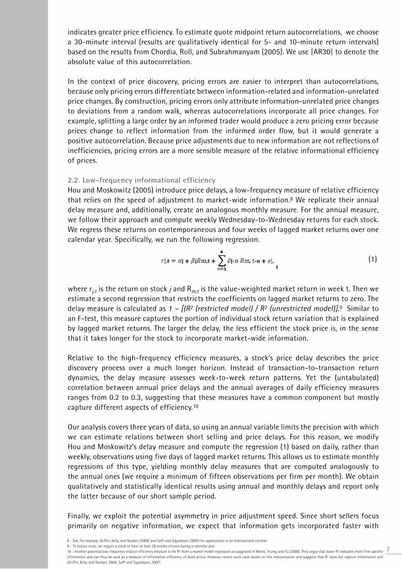
2.2. Low-frequency informational efficiencyHou and Moskowitz (2005) introduce price delays, a low-frequency measure of relative efficiency that relies on the speed of adjustment to market-wide information.8 We replicate their annual delay measure and, additionally, create an analogous monthly measure. For the annual measure, we follow their approach and compute weekly Wednesday-to-Wednesday returns for each stock. We regress these returns on contemporaneous and four weeks of lagged market returns over one calendar year. Specifically, we run the following regression.

(1)

where rj,t is the return on stock j and Rm,t is the value-weighted market return in week t. Then we estimate a second regression that restricts the coefficients on lagged market returns to zero. The delay measure is calculated as 1 – [(R2 (restricted model) / R2 (unrestricted model)].9 Similar to an F-test, this measure captures the portion of individual stock return variation that is explained by lagged market returns. The larger the delay, the less efficient the stock price is, in the sense that it takes longer for the stock to incorporate market-wide information.

Relative to the high-frequency efficiency measures, a stock’s price delay describes the price discovery process over a much longer horizon. Instead of transaction-to-transaction return dynamics, the delay measure assesses week-to-week return patterns. Yet the (untabulated) correlation between annual price delays and the annual averages of daily efficiency measures ranges from 0.2 to 0.3, suggesting that these measures have a common component but mostly capture different aspects of efficiency.10

Our analysis covers three years of data, so using an annual variable limits the precision with which we can estimate relations between short selling and price delays. For this reason, we modify Hou and Moskowitz’s delay measure and compute the regression (1) based on daily, rather than weekly, observations using five days of lagged market returns. This allows us to estimate monthly regressions of this type, yielding monthly delay measures that are computed analogously to the annual ones (we require a minimum of fifteen observations per firm per month). We obtain qualitatively and statistically identical results using annual and monthly delays and report only the latter because of our short sample period.

Finally, we exploit the potential asymmetry in price adjustment speed. Since short sellers focus primarily on negative information, we expect that information gets incorporated faster with

78 - See, for example, Griffin, Kelly, and Nardari (2009) and Saffi and Sigurdsson (2007) for applications in an international context.9 - To reduce noise, we require a stock to have at least 20 weekly returns during a calendar year.10 - Another potential low-frequency relative efficiency measure is the R2 from a market model regression as suggested in Morck, Yeung, and Yu (2000). They argue that lower R2 indicates more firm-specific information and can thus be used as a measure of information efficiency of stock prices. However, recent work casts doubt on this interpretation and suggests that R2 does not capture information well (Griffin, Kelly, and Nardari, 2009; Saffi and Sigurdsson, 2007).

8

more shorting when market-wide information is negative. We modify the above unrestricted models by separating positive and negative market returns.

(2)

(3)

where equals the market return when it is either positive or zero, and equals the market return when it is negative. We then use the R2 from the modified unrestricted model in the denominator to calculate two delay measures that separately capture price adjustment to positive and negative information.

2.3. Post-earnings announcement driftPost-earnings announcement drift is a well-established financial phenomenon that indicates some degree of informational inefficiency in the capital markets. Ball and Brown (1968) first document that abnormal returns of stocks with positive earnings surprises tend to remain positive for several weeks following the earnings announcement, and remain negative for stocks with negative surprises. This return pattern generates an arbitrage opportunity for savvy traders. If short sellers are sophisticated traders who attempt to exploit this opportunity, we expect increased shorting immediately following negative earnings surprises and decreased shorting following positive surprises. If short sellers make prices more informationally efficient, the increased shorting activity following negative surprises should attenuate the post-earnings announcement drift. We use this event-based test to supplement our previous two measures of informational efficiency.

Battalio and Mendenhall (2005) and Livnat and Mendenhall (2006) show that earnings surprise measures based on analyst forecasts are easier to interpret than the ones obtained from a time series model of (Compustat) earnings, because the former are not subject to issues such as earnings restatement and special items. We compute earnings surprises as the difference between actual earnings and the most recent monthly I/B/E/S consensus forecasts, scaled by the stock price two days before the announcement date. We construct abnormal returns as a stock’s raw returns net of value-weighted market returns, and measure the drift as the cumulative abnormal returns following each earnings surprise.

2.4. Return reversals at the daily frequencyOpponents of unrestricted short selling often allege that short selling puts excess downward pressure on prices.11 As a result, these opponents claim, prices are too low relative to fundamental values when short sellers are active. A related allegation is that short sellers can manipulate prices by shorting intensely, thereby driving prices down below their efficient values. Once these stocks are undervalued, the short sellers could then cover their positions as the true valuations are slowly revealed and prices reverse towards their efficient values. Both of these scenarios imply that short sellers are more active on days when prices decline, and especially so when these declines are not related to fundamental information. We provide evidence on this issue by selecting large price moves and looking at short sellers’ behavior around these extreme return days.

3. Shorting flow and the short-horizon efficiency of transaction prices Relative short-horizon efficiency describes how closely transaction prices follow a random walk, and we estimate how short selling flow affects the degree of short-term efficiency. We regress

11 - For public concerns or issuers’ comments, See SEC Release No. 34-58592 or the NYSE survey on short selling (“Short selling study: The views of corporate issuers”, Oct 17, 2008 at http://www.nyse.com/press/1224497730781.html).

daily measures of short-term efficiency on lagged shorting and control variables. Because the relevant measures of efficiency and shorting are available at the daily frequency, these tests are quite powerful. We use the following basic model to test hypotheses about short selling on efficiency: Efficiencyi,t = αt + βt Shortingi,t-1 + γt Controlsi,t-1 + εi,t (4) The dependent variable is either the pricing error, σ(s)/σ(p), or the absolute value of midquote return autocorrelation, |AR30|. Following Boehmer, Jones, and Zhang (2008), we standardize daily shorting flow by the stock’s daily share trading volume. This standardization makes shorting activity comparable across stocks with different trading volume. If more shorting systematically contributes to greater price efficiency, stock prices should deviate less from a random walk, implying a negative β. We lag explanatory variables by one period to mitigate any potential influence of changes in price efficiency on these contemporaneous explanatory variables.12

Research suggests several control variables that are potentially associated with price efficiency. We include measures of execution costs, share price, market capitalization, and trading volume as controls in our base regressions. To measure execution costs, we use relative effective spreads (measured as twice the distance between the execution price and the prevailing quote midpoint scaled by the prevailing quote midpoint).13 Higher execution costs make arbitrage less profitable, and therefore deter the entrance of sophisticated traders whose trading helps keep prices in line with their fundamentals. This reasoning suggests that stocks with higher trading costs tend to deviate more from their fundamental values, and thus are less efficiently priced. We include the volume-weighted average price (VWAP) to control for differences in price discreteness that can potentially affect efficiency.14 Larger and more actively traded stocks may be easier to value. Moreover, Chordia and Swaminathan (2000) show that, after controlling for size, high-volume stocks tend to respond more quickly to information in market returns than do low-volume stocks. Thus, we include both variables in our models. Because the natural logs of trading volume and market capitalization are highly correlated (the correlation coefficient is 0.75), we orthogon alize volume with respect to size. Specifically, throughout the paper, we use residuals from regressing log volume on log of market capitalization. Results remain qualitatively similar without this orthogonalization. We include the lagged dependent variable to control for potential persistence in relative price efficiency.15

Recent literature suggests two additional important variables that should be considered in studying price efficiency. First, because analyst coverage can improve a firm’s informational environment, we control for the number of sell-side analysts (Brennan and Subrahmanyam, 1995). We obtain the monthly number of analysts producing annual forecasts from I/B/E/S. Second, Boehmer and Kelley (2009) find that institutional investors contribute to greater informational efficiency. We control for institutional holdings so we can focus on marginal effect of shorting over and above the effect of institutional holdings. As in Boehmer and Kelley, we use holdings from the 13F filings in the CDA Spectrum database standardized by a firm’s shares outstanding.

3.1. Descriptive statisticsPanel A in Table 1 presents time-series means of cross-sectional summary statistics for these variables. Relative shorting volume accounts for close to 20% of total trading volume during the sample period. A 10% standard deviation reveals large variation in shorting activity across stocks. Price efficiency measures also exhibit substantial cross-sectional variation. Variables such as firm size, trading volume, share prices, and number of analysts are skewed, and we use their natural logarithms in our estimation.

9

12 - The lagged explanatory variables can be interpreted as instruments for their contemporaneous values. Results using contemporaneous values are qualitatively the same.13 - Controlling for relative effective spreads serves another purpose in the pricing error regression. The pricing error reflects the information-uncorrelated (i.e. temporary) portion of total price variance. Since the effective spread measures the total price impact of a trade and thus could conceivably be related to the pricing error, controlling for it can help isolate changes in efficiency from changes in liquidity. 14 - Using closing prices produces qualitatively identical results. 15 - While price volatility is conceivably related to short-term efficiency, both of our dependent variables are already scaled by a volatility measure. Therefore, we do not add volatility as an explanatory variable to the model.

1016 - Results are not sensitive to other reasonable lag lengths for Newey-West standard errors.17 - The dependent variable in Models 1 and 2 in Table 2 is the ratio σ(s)/σ(p). Thus, the efficiency-enhancing effect of short selling could conceivably arise only because shorting inflates σ(p), the standard deviation of share prices over time. We can dismiss this possibility empirically. In unreported regressions similar to Model 2, but with σ(s) as the dependent variable, we find that the coefficient on lag shorting is significantly negative even when we control for σ(p). Thus, an increase in shorting tends to reduce the pricing error per se.

Panel B in Table 1 reports time-series averages of monthly cross sectional correlations between shorting and price efficiency. The three measures of informational efficiency are positively correlated. Correlations range from 0.07 (between delay and |AR30|) to 0.23 (between delay and pricing error). This suggests that these three measures have a common component but mostly capture different aspects of price efficiency. But each of the three price efficiency measures is negatively related to shorting, which provides initial evidence that short selling is associated with greater relative price efficiency. Of course, these correlations are only suggestive and we conduct more rigorous tests to formalize this observation.

3.2. Basic resultWe employ a standard Fama and MacBeth (1973) two-step procedure to estimate model (4). In the first stage, we run daily cross-sectional regressions of price efficiency on shorting activity and controls. In the second stage, we draw inferences from the time-series average of these regression coefficients. This method picks up the cross-sectional effect of shorting on price efficiency, and is less susceptible to cross-sectional correlations among regression errors than a pooled cross-sectional time series regression. To correct for potential autocorrelation in the estimated coefficients, we use Newey-West standard errors with five lags.16

Table 2 contains the regression results. Models 1 and 2 use pricing errors as the efficiency measure, while models 3 and 4 use Ln|AR30|. For each measure, we present the base model and a model augmented by the number of analysts and institutional holdings. Lagged daily shorting flow has a significant and negative coefficient in each of these specifications. This means that controlling for other factors, greater shorting flow is associated with smaller pricing errors and smaller autocorrelation and thus faster price discovery. In other words, short selling is associated with prices that deviate less from a random walk and hence are more informationally efficient.17

The coefficients of most control variables exhibit the expected signs. Larger relative effective spreads are associated with larger pricing errors. This makes sense because higher spreads prevent some arbitrageurs from immediately jumping on temporary price deviations, and therefore lead to lower efficiency. Larger and more actively traded stocks are also associated with smaller pricing errors.

Consistent with prior literature, greater analyst coverage and more institutional holdings promote efficiency (Boehmer and Kelley, 2009). To put these effects into perspective with the effect of short selling, we compare the relative influence of institutional holdings, analyst coverage, and short selling. Specifically, in Model 2, a one-standard-deviation (0.0992) increase in short selling is associated with a 0.0043 decline in pricing errors. A one-standard-deviation increase in LnNumEst100 and InstOwn is associated with pricing error reductions of 0.0014 and 0.0048, respectively. Based on this comparison, variation in short selling has a similar effect on efficiency as variation in institutional holdings. At the same time, both shorting and institutional holdings are more than three times as influential for price efficiency than analyst coverage is. Overall, these comparisons illustrate that short selling is an important driver of price discovery. In the next sections, we show that this basic result is statistically and economically robust and insensitive to different measures of price discovery.

3.3. Exempt vs. non-exempt short sellingThe analysis in the previous section lumps together all short sellers, but theoretical work on short selling (Diamond and Verrecchia, 1987; Bai, Chang and Wang, 2006) models the behavior of informed short sellers differently from that of uninformed short sellers. This section attempts to shed some light on how different information is related to the effect shorting has on price efficiency.

While one cannot directly distinguish informed from uninformed short sellers, the NYSE shorting data have a unique feature that helps differentiate, to some extent, motivations for short selling. Specifically, we observe an indicator that identifies shorts that are exempt from the uptick rule. Exempt shorting primarily includes market-making activities. Shorting in the course of market making, by definition, should have less information content as shorting by other traders. Other things equal, we thus expect non-exempt shorting to contribute more to price discovery, and, therefore, to have a stronger efficiency-enhancing effect than exempt shorting. One technical issue complicates this test. After Reg SHO is implemented on May 2, 2005, the uptick rule ceases to apply for a subset of stocks (the “pilot stocks”).18 These stocks are intentionally exempt from the uptick rule, making the “exempt” marker redundant. Reg SHO specifies that all short sales in these pilot stocks should be marked as “exempt.” As a result, an “exempt” indicator in pilot stocks no longer unambiguously indicates market-making shorts as before. For these reasons, our analysis in this section is limited to non-pilot stocks and ends on July 5, 2007.19

Non-exempt shorting (on average 18% of trading volume) clearly dominates exempt shorting (on average 0.7% of volume) on the NYSE. To investigate the differential effect of exempt shorting on the informational efficiency of prices, we decompose shorting in equation (4). Model (1) in Table 3 reports the corresponding Fama and MacBeth (1973) two-step regression results. The efficiency-enhancing effect of short selling arises entirely from non-exempt shorting. Stocks with more intense non-exempt shorting have significantly smaller pricing errors (and return autocorrelations, which are not shown in the Table). In contrast, exempt shorting does not reduce pricing errors (or the absolute value of return autocorrelations). Consistent with our conjecture, this suggests that non-exempt short selling is at least partially motivated by information, and thus aids price discovery by improving the informational efficiency of share prices. Taken together, these results plausibly suggest that short sellers only improve the informational efficiency of prices if their trades are information motivated.

3.4. The effect of short selling constraintsWhen traders face shorting constraints, theory tells us that negative information is not fully incorporated into prices (Miller, 1977) or more slowly (Diamond and Verrecchia, 1987) than without shorting constraints. This slows price discovery and we expect the informational efficiency of prices to decline with the severity of shorting constraints. We conduct two supplemental experiments in this regard. First, we look at the regulator-designed experiment associated with Reg SHO between 2005 and 2007, which exempted a stratified sample of stocks from the uptick rule (see footnote 18). We compare the effect of shorting pilot stocks (not subject to the uptick rule) to the effect of shorting in the non-pilot stocks during the same period. Second, it is widely accepted that stocks with low institutional holdings are harder to borrow, and hence more difficult to short than stocks with more institutional holdings (see Nagel, 2005; Asquith, Pathak, and Ritter, 2005). Similarly, industry representatives often argue that stocks priced below $5 are more difficult to short because of frictions including higher margin requirements. We look at these effects and their interactions to assess how shorting restrictions relate to price discovery.

We report the results in Table 3. Model 2 allows intercepts and the short selling slope coefficient to vary with changes in the uptick rule.20 More specifically, we add four new variables: a pilot dummy indicating pilot stocks; a post dummy indicating the period over which price tests were removed for pilot stocks; and an interaction pilot*post*Shorting.

The main results from Table 2 still hold. First, the period of the Reg SHO pilot appears to be associated with a secular decrease in informational efficiency, because post has a significantly

11

18 - The SEC selected pilot securities from Russell 3000 index as of June 25, 2004. First, 32 securities in the Russell 3000 index that are not listed on the American Stock Exchange (Amex), or on the New York Stock Exchange (NYSE), or not Nasdaq national market securities (NNM) are dropped. Securities that went public after April 30, 2004 are also excluded. The remaining securities are then sorted into three groups by marketplace, and ranked in each group based on average daily dollar volume over the one year prior to the issuance of the order. From each ranked group, SEC selected every third stock to be a pilot stock starting from the 2nd stock. The remaining stocks are suggested to be used as the control group where the price test restriction still applies. Of all pilot stocks, 50%, 2.2% and 47.8% are from NYSE, Amex, and Nasdaq NNM, respectively. For more information about Reg SHO, see SEC Release No. 50104/July 28, 2004. See Diether, Lee, and Werner (2009) and Alexander and Peterson (2008) for analyses of short selling around this event.19 - The SEC eliminated the uptick rule on all stocks on July 6 2007. See SEC Release No.34-55970.20 - Because the SEC eliminates the uptick rule for all stocks on July 6 2007, our sample for this analysis includes pilot stocks and control stocks from January 1, 2005 to July 5, 2007.

12

positive coefficient. It is not clear whether this change is related to the Reg SHO pilot or not. More importantly, the efficiency-enhancing effect of short selling becomes stronger in the Pilot stocks: the coefficient on the interaction is significantly negative, and represents a 50% increase in the efficiency-enhancing effect of short selling, compared to control stocks during the same period. Second, both episodes with stock prices below $5 and institutional holdings below 5% are associated with significantly worse price discovery. Comparing these effects to the overall effects of shorting on efficiency, being in the hard-to-short categories reduces the efficiency-enhancing effect of short selling by about 85%.21 Overall, these additional results show that shorting aids price discovery the most when traders are well informed and shorting constraints are not binding.

4. Short selling flow and price delaysChordia, Roll, and Subrahmanyam (2005) point out that price discovery occurs mainly within a trading day and Boehmer and Kelley (2009) find evidence in this direction. But if prices diverge from fundamentals for periods longer than one day, such intraday analysis could erroneously interpret “riding the bubble” behavior as short-term reversion to fundamentals. For this reason alone it is important to assess the effect of short selling on informational efficiency measured over longer horizons. In this section, we examine how shorting affects price delays, an efficiency measure estimated at monthly and annual horizons. Price delays reflect the sensitivity of a firm’s returns to contemporaneous and lagged market returns and measure how quickly market-wide information is incorporated into stock prices (Hou and Moskowitz, 2005). To make the results comparable to those in the main tests in Table 2, we include similar control variables in the regression. The main difference is that a daily panel underlies Table 2, while a monthly panel underlies the price delay tests. In Table 4, we present both monthly Fama-MacBeth and two-way fixed effect models. Despite its low power we obtain qualitatively identical results using an annual panel (as originally suggested in Hou and Moskowitz, 2005).

We report three sets of regressions in Table 4. Panel A shows regressions explaining the basic monthly delay measure. We explain delays associated with negative news in Panel B and delays associated with positive news in Panel C. Short selling significantly attenuates price delays in each of the three panels, for both the Fama-MacBeth and the fixed effect models. This suggests that stocks with more shorting activity incorporate public information significantly faster into prices than those with less shorting. This holds for both positive and negative public information, and more strongly for negative information. This finding substantiates the core result that shorting enhances the informational efficiency of prices, because price delays capture a dimension of the price discovery process that is quite distinct from the one that underlies our transaction-based short term approach in Table 2.

5. Short selling and post-earnings announcement driftReturns tend to be positive after positive earnings surprises and negative after negative surprises–in other words, prices seemingly do not fully incorporate earnings-related information at the time of the announcement (see Ball and Brown, 1968). Bernard and Thomas (1989, 1990) suggest that such post-earnings announcement drift (PEAD) is a manifestation of investors’ failure to recognize the information in the earnings surprises. Since prices tend to drift upwards (downwards) following a positive (negative) earnings shock, this predictable pattern creates a potential arbitrage opportunity for savvy traders. We have two hypotheses about short selling in the context of PEAD. First, if short sellers are sophisticated traders who attempt to exploit this opportunity, we expect more shorting immediately following negative earnings surprises. Second, if short sellers enhance efficiency, the shorting activity after negative surprises should attenuate PEAD. After looking at short-term and long-term measures of informational efficiency, 21 - For example, for low-priced stocks, the coefficients on shorting and the low-price dummy imply that the efficiency-enhancing effect declines to (.0405-.0351)/.0405=.13 of the original unconstrained effect. The interactive effect partially outweighs this change in the case of low-priced stocks, because the marginal effect of short actually increases. This means that the smaller amount of shorting that is still possible in low-priced stocks may be particularly informative. We find no significant interaction effect for stocks with low institutional holdings.

this event-based test is our third main approach to examining the relation between shorting and the price discovery process.

In this section we report some descriptive statistics for shorting around both positive and negative earnings surprises, but we concentrate our analysis on the response of short sellers to negative surprises. We do this because it is not clear how to interpret changes in short selling after positive surprises. For example, suppose short sellers know the true value of a stock and observe that the market underreacts to the negative information in an earnings announcement. Then traders would short more intensely to take advantage of this arbitrage opportunity, and our test is designed to detect this change in shorting activity. But if short sellers observe that the market underreacts to the positive information in an announcement, they can react in two ways–either reduce shorting, or increase purchases. But more likely than not traders do not have a short transaction planned for this day, and thus it is more likely that the response will be more intense purchases, rather than less intense shorting. Unfortunately we cannot observe the long transactions of the short sellers in our sample, which makes the effects of short selling around positive surprises hard to interpret. For this reason, we concentrate our analysis in this section on negative earnings surprises.

Our sample covers 15,536 earnings announcement events. We use a simple portfolio approach to examine how short sellers respond to earnings surprises. Specifically, each quarter, we sort firms into quartile portfolios according to the earnings surprise measures, with quartile 1 containing stocks with the most negative surprises and quartile 4 those with the most positive surprises. To check whether PEAD is present during our sample period, we compute announcement-related cumulative abnormal returns (CARs), defined as a stock’s raw return minus the value-weighted market returns. Table 5 reports equally weighted CARs for each quartile. Consistent with prior findings, the announcement effects are very strong: abnormal returns during the three-day window (-1, 1) centered on the announcement date are large and negative (-3.26%) for portfolios with the most negative surprises, and large and positive (3.40%) for positive surprises. More importantly, we observe significant PEAD for each but the third largest surprise quartile: prices of stocks with good (bad) surprises continue to drift upwards (downwards) after the announcement. Finally, PEAD is monotonic across quartiles–one-week cumulative abnormal returns starting from the second day after the announcement date (2, 6) increase monotonically from -0.75% for stocks with the most negative surprises to 0.42% for stocks with the most positive surprises.

We now address our hypotheses, that (1) short sellers view the drift period as a mis-pricing episode and trade accordingly, and (2) this promotes price discovery. If short sellers understand and seek to exploit the arbitrage opportunity associated with post-earnings announcement drift, they would short more intensively stocks in quartile 1 right after observing the market reaction to the announcement. To the extent short sellers have previously planned to trade on or after the announcement, they would reduce their shorting activity in stocks with positive surprises (quartile 4) if they view the announcement return as too small.

We first look at shorting and returns graphically in Figure 1. Panel A shows CAR and shorting for negative surprises (Q1). We make several interesting observations. First, shorting increases from about 19.8% of volume at t-2 to about 21.5% at t +1 for the most negative surprises (Q1). This pattern is also statistically significant: the change in shorting from (-6,-2) to (+2,+6) around the announcement date is 1.28% for Q1 and 0.28% for Q2, and both are statistically significant at the one-percent level (not tabulated). Second, the main adjustment to shorting activity for Q1 occurs on the day after the announcement, so it is likely that short sellers’ indeed react to the information and corresponding market reaction on that day. Both of these observations support our first hypothesis. Furthermore, daily returns move in the direction of the change in shorting: for increases in shorting, we observe a contemporaneous negative return.

13

14

In Panel B, we split the Q1 sample based on the change in shorting from the week before the announcement to the week after (more precisely, the change from (-6,-2) to (+2,+6) relative to the announcement date). High-shorting events are thus Q1 announcements with an above-median change in shorting, and conversely for low-shorting events. Both the high-shorting and low-shorting portfolios are associated with large negative returns after the announcement, but drift is eliminated only in the high-shorting portfolio. While we can only speculate why short sellers do not increase shorting in the low-shorting portfolio, the finding that PEAD goes away when short sellers choose to become more active supports our main conclusion so far: short sellers help the price-discovery process and make prices more informationally efficient.22

The finding that PEAD vanishes after negative earnings surprises with large increases in short selling is consistent with our second hypothesis. We now present a more formal test related to this finding. Each quarter, we sort stocks into quartiles based on earnings surprises. Within each earnings surprise quartile, we again partition stocks into two groups based on changes in shorting activity around the announcement. Table 6 reports one- and two-week post-earnings announcement drift for this double sort for negative surprises. Again, the evidence suggests that increase in shorting enhance efficiency, in this case by reducing the drift. Using the one-week drift, stocks with very negative earnings surprises (Q1) and large increases in shorting exhibit no drift–the post-announcement CAR is 11bp and not statistically different from zero. In contrast, the corresponding low-shorting portfolio experiences a drift of -154bp. It is not entirely clear to us why short sellers do not arbitrage this 154bp drift in the same way as they remove the drift in the high-shorting portfolio. But even with a return this large it is possible that it is not sufficient to cover round-trip transaction costs, because traders must short into a declining market to take advantage of this temporary mis-pricing (unfortunately, we cannot observe the return that would have accrued to the high-shorting portfolio had the shorting not increased). If expected transaction costs are high, arbitrage is risky ex ante and this may prevent traders from incurring a larger short position designed to take advantage of the drift. Alternatively, PEAD could arise partly because prices are slow to adjust, and partly because of other reasons that do not involve mispricing (Sadka, 2006). In this case, short sellers can only arbitrage the drift in the former case. But in the high-shorting group traders do bring prices closer to fundamentals, and we obtain almost identical results for the two-week window. Overall, these event-based results provide additional support for the hypothesis that short sellers help make prices more efficient.

As a last test of the effect of shorting on PEAD, we recognize that other factors also contribute to the magnitude of PEAD. To estimate the effect of shorting goes beyond the influence of those other factors, we estimate the following multiple regression:

(5)

The dependent variable is the cumulative market-adjusted abnormal return from day 2 to day 6. DUE represents the scaled decile ranking of earnings surprises (Bartov, Radhakrishman and Krinsky, 2000). Specifically, each quarter, we sort unexpected earnings into deciles and scale decile ranks to range between zero (most negative earnings surprises) and one (most positive earnings surprises). With non-zero PEAD, we expect a positive coefficient on β1. To estimate the marginal effect of shorting on the slope of DUE, we include DUE*D∆SS, the interaction between DUE, and a scaled decile rank variable representing changes in daily average shorting activity from (-6, -2) to (+2, +6) around earnings announcements. Specifically, each quarter, we sort in descending order the change in shorting activity. We form deciles and scale the ranks to range from zero (largest increase in shorting) to one (largest decrease in shorting). If short sellers attempt to exploit PEAD and have an effect on post-announcement prices, β2 should be negative: firms with negative earnings surprises and a greater increase in shorting should exhibit smaller drift.

22 - The firms in the low-shorting Q1 portfolio are not substantially different from firms in the high-shorting Q1 portfolio along dimensions that are commonly associated with shorting difficulty, such as price level and institutional holdings. Moreover, none of the results in this section is sensitive to the presence of the uptick rule–results are qualitatively identical for pilot and non-pilot stocks.

We include additional controls suggested in the literature. Following Bartov, Rashakrishman, and Krinsky (2000), all controls are in the form of decile ranks interacted with DUE. Bartov et al. and Ke and Ramalingegowda (2005) show that institutional investors are sophisticated investors who exploit earnings patterns, so we include last-quarter institutional holdings scaled by shares outstanding as a control. We also include several variables that proxy for liquidity, which may be associated with earnings drift (Chordia et al., 2009; Sadka, 2006). These liquidity proxies include dummy variables of the average daily turnover one week prior to the announcement (DTO), and firm size last quarter (DSize).23

Table 7 reports the regression results. Consistent with our expectations, the coefficient on DUE is significantly positive, suggesting that negative earnings surprises are followed by downward drift. Institutional ownership is not significant, possibly due to a relatively short sample period with low frequency of data. Turnover, as a proxy for liquidity, significantly reduces drift, consistent with Chordia, et al (2009) and Sadka (2006). Our key variable, DUE*D∆SS, is significantly negative across all model specifications. So PEAD is significantly smaller when short sellers act on arbitrage opportunities associated with PEAD, beyond the effect that cross-sectional differences in liquidity have. In the process of arbitraging PEAD, short selling activity improves the informational efficiency of prices.

6. Short selling and extreme price movementsIn general, short sellers tend to be contrarians who sell more after periods of positive returns (Diether, Lee, and Werner, 2008). But some studies also provide evidence that, under specific circumstances, some short sellers can destabilize prices by driving prices away from efficient values. For example, Shkilko, Van Ness, and Van Ness (2007) find that some short sellers drive down prices too far during extreme price declines. Similarly, Henry and Koski (2010) argue that short sellers are able to push prices too far down just before seasoned equity offerings. While the objective of our paper is to assess the effect of short sellers as a group, rather than a subset who may exploit extreme return events or specific corporate actions, it is useful to extend our analysis in this direction. More specifically, we look at short selling around large price moves, and, in particular, around daily price reversals. By definition, price reversals typically involve no new information–otherwise the price change should be permanent.

Analysis of these no-information events can shed some light on two central issues in the short selling debate: whether short sellers cause the no-information price declines, and whether or how short sellers react to no-information price declines. Regarding the first issue, the SEC is expressly concerned that short selling may cause “sudden and excessive fluctuations of the prices.”24 If nefarious short sellers destabilize prices, we expect more intense shorting on down days, especially when the downward price change is unrelated to fundamental information. In contrast, if short sellers help to keep prices in line and close to their efficient values, we expect them to short less on extreme down days and short more on extreme up days, especially when these initial price shocks are unrelated to fundamental information. Regarding the second issue, short sellers reaction to extreme price moves, we could expect nefarious shorters to increase shorting after observing large downward price changes in the hope of covering at still lower prices. In contrast, efficiency-enhancing short sellers would reduce sales after observing no-information price declines and gain from the impending reversals. Similarly, these short sellers would increase shorting after observing large, no-information price increases.

To identify extreme return days for each stock, we select days with returns exceeding two standard deviations, measured over the past 20 trading days. Then we classify these events into one of four categories, depending on what happens on the next day: a continuation, a small reversal, a large reversal, or an overshooting reversal. For example, if we have a large negative return on day t, a

1523 - We also use quartile ranks instead of decile ranks, and above/below median dummies in shorting change. This leaves the results qualitatively unaltered and largely reproduces our double sorts results as well.24 - See SEC Release No. 34-58592.

16

continuation is any non-positive return on day t+1. A reversal of less than 20% of the down-day’s return would be classified as a small reversal, and one that reaches more than 20% but remains below the closing price on day t-1 is a large reversal. An overshooting reversal means that the price on day t+1 closes above the closing price on day t-1. We proceed analogously for extreme positive returns events.

To make inferences about short sellers’ contributions to price discovery around these extreme events, we exploit our ex post knowledge that returns around reversals are at least partially transient. Because information events would lead to permanent price adjustments, reversals tend to be unrelated to information. Such a no-information price reversal could arise, for example, when a large passive fund experiences outflows and thus becomes obliged to sell a larger quantity of shares. This would temporarily lower prices to induce other traders to buy these shares. Once the selling pressure subsides, in the absence of stock-specific negative information, prices would then return to the level prior to the large sell. If short sellers are smart traders who understand that the initial negative return is transient, we expect them to reduce their shorting while prices are (temporarily) below their efficient values. In contrast, for temporary positive price shocks, we expect short sellers to increase shorting while prices are elevated. This background allows us to make inferences without having to assume that short sellers trade on private information about fundamental values. Instead, we make the weaker assumption that, conditional on observing a large price change, short sellers can distinguish information-based price changes from those that are later reversed.

Figure 2 (extreme negative returns) and Figure 3 (extreme positive returns) summarize the behavior of short sellers around these different return events. Each figure contains four panels, corresponding to the categories of price behavior on day t+1. We present results using daily raw returns, but the graphs look very similar when we use market-adjusted returns to identify extreme return events and subsequent price reactions. As before, we measure shorting as a percentage of contemporaneous trading volume.

We first examine shorting around the large negative day t returns in Figure 2. The price drop averages about 4-5% across the four panels. By construction, the shock in Panel A experiences a continuation on the next day and we do not know if the returns are eventually reversed or not or whether new information is partly responsible for these events. We show the continuation graphs for completeness. But because the negative returns in Panels B through D reverse on the next day, we know that the corresponding t=0 returns are transient, and we can investigate whether short sellers trade as if they understand that they are not information based. If shorters attempted to manipulate prices or exacerbate price declines for these reversals, we would expect shorting to increase either on the down day or before. None of the graphs supports this conjecture: shorting is fairly flat before the drop in all cases and then declines dramatically on the day of the price decline. This suggests that short sellers, as a group, recognize the price decline as temporary and reduce their selling activity accordingly. The decrease in shorting alleviates downward pressure on prices and should result in smaller declines than we would have observed had short sellers not changed their trading activity.

Next, we look at the day t+1 returns. In Panel A, these returns are negative; in all other panels, they are positive and, by construction, these returns increase monotonically from Panel A to Panel D relative to the day t price decline. If the extreme price declines on the previous day are temporary and shorters interpret them correctly, we would expect shorting on day t+1 to increase with the magnitude of the reversal. For example, if prices reverse partially (Panel B), informed short sellers may expect further reversal and limit their trading activity. In Panel D, we expect informed short seller to trade more intensely during and after the overshooting reversals because, if there is no new information, prices have increased too much. The day t+1 results support this conjecture. In Panel A, price declines continue and shorting remains low. On days with small reversals (Panel B),

short selling increases slightly from day t, but remains substantially lower than before the shock for the next five trading days. On days with large reversals (Panel C), short sellers resume their pre-event activity level quickly. Finally, for the overshooting returns (Panel D), short sellers increase their shorting activity the most. Notably, day t+1 shorting activity is monotonically related to the reversal magnitude: we observe more short selling relative to pre-event means as we move from Panel A to Panel D. Each of these observations is consistent with the view that short sellers trade to keep prices in line with their efficient values.

Figure 3 repeats this analysis for the opposite event (extreme positive returns, further classified into four categories according to t+1 returns). As we would expect for shorters who view the positive return as transient, the day t price increases are associated with a substantial increase in shorting activity in each case. This is consistent with the contrarian nature of short selling (see Diether, Lee, and Werner, 2008). Equally important, and similar to Figure 2, we find that shorting on day t+1 is monotonically related to the magnitude of return reversals. Shorting is highest when prices continue to increase (Panel A) and lowest when prices fall below their day t-1 level (Panel D).25

Overall, these results are consistent with Diether, Lee, and Werner’s (2008) finding that short sellers act as contrarians.26 In addition, we show that short sellers’ trading helps to accelerate price discovery during these extreme events. Shorters sell more when prices jump unusually high, and they short less when prices drop unusually low, and they swiftly change their behavior as prices reverse. Moreover, for extreme returns that are reversed on the next day, short sellers appear to recognize the temporary nature of these price swings. As a result, their trading provides liquidity to the market and keeps prices in line, even during these volatile episodes.

7. Robustness Our key finding is that short sellers facilitate price discovery and make prices more informationally efficient. We provide evidence along four dimensions of efficiency by looking at how short selling relates to deviations of transaction prices from a random walk, low-frequency price delays, post-earnings announcement drift in event time, and non-information based large price movements. We view the transaction-based analysis as the strongest convincing argument in this set and discuss additional sensitivity test tests in this direction.

7.1. Distribution of shorting flowShorting flow is highly skewed. To assure that distributional issues do not affect our results, we use decile ranks in place of shorting flow to test for efficiency effects. Specifically, on each day, we sort stocks into deciles based on the prior day’s relative shorting volume. Then we use the decile ranks in regression model (4). This approach reduces the influence of outliers on the estimates. Our main finding (not tabulated) remains unchanged with this alternative shorting measure: stocks ranked higher in terms of relative shorting flow are associated with significantly smaller values of both pricing errors and return autocorrelations.

7.2. Influence of unobservable firm effectsOur high-frequency results may also be affected by firm-specific effects. To address this possibility, we construct a measure of “abnormal” shorting. Each day, we compare a stock’s relative shorting volume to its own moving average over the past week to determine whether shorting has become more or less intense. This way we identify stocks that experience a shock in their own shorting activity and take into account potential persistence in a firm’s shorting activity. Another way of

17

25 - In robustness tests that we do not tabulate, we repeat the analysis in Figures 2 and 3 after excluding earnings announcement dates from these extreme return events. The results remain the same. We also examine pilot and control stocks separately for these extreme return events, and the general patterns hold for both. These robustness tests suggest that neither earnings news nor mechanical issues related to the tick test drive our results in this section.26 - Using a similar sample (largely the first half of our sample period), Shkilko, Van Ness, and Van Ness (2007) argue that short sellers worsen price declines. This is at odds with the results we report in Figures 2 and 3. One potential reason for the difference is that Shkilko et al. look at 5-minute intraday cumulative returns. At the five-minute frequency, it is not clear what distinguishes potentially manipulative price effects from ordinary temporary price impacts that are typically associated with any type of order flow. Another, more likely, reason is that they use a different measure of shorting activity. Their measure weights changes in shorting in the cross-section by the inverse of volatility of the stock-specific time series of short selling. Because the most informed shorting flow will tend to be the most volatile, their measure gives large weight to uninformed shorting and little weight to informed shorting. In this paper, in contrast, we weight equally across firms. In this sense, our results are not inconsistent with Shkilko et al.’s, because it is not surprising that the least informed short sellers do not improve efficiency.

18

addressing stock fixed effects is to model them directly in a panel regression. This methodology mitigates the omitted-variable concern with cross-sectional OLS regressions. Both the abnormal-shorting tests and the fixed-effect panel regressions produce qualitatively identical results (not tabulated): stocks with higher abnormal shorting are priced more efficiently as observed by smaller pricing errors and autocorrelations.

We also consider additional controls. One variable that may be related to price (in)efficiency is one-sided trading pressure. If excess demand or supply is not immediately absorbed by liquidity providers on the other side of the imbalance, less efficient prices may result. If short selling is related to the degree of one-sided trading pressure in either direction, our results may not reflect the effect of shorting but rather that of other large traders. We control for this possibility by including the absolute value of order imbalances in the regressions. The coefficient for this variable is positive in all specifications (i.e., imbalance is associated with less efficient prices) and significant in some specifications, but it does not drive away the effects shorting has on efficiency. We also include lagged two-week returns to control for short-term momentum. Again, the inclusion of this variable does not remove the effect of shorting on price efficiency. We use turnover in place of log volume in the regressions. To the extent that turnover serves as a proxy for investor attention (Chordia and Swaminathan, 2000), it could be related to price efficiency since high-volume stocks tend to respond more quickly to information in market returns than do low-volume stocks. We find that increased turnover makes prices more efficient, but shorting remains significant as well.27

7.3. Reverse causalityReverse causality is an important issue that we have not yet addressed. It is important, because a plausible story links efficiency to shorting. Institutional investors may prefer to hold efficiently priced stocks because they are less likely to be mispriced. But stocks with higher institutional holdings are also easier to short (Nagel, 2005), because the supply of lendable shares is greater in these stocks. Therefore, efficiently priced stocks may exhibit more shorting activity. If efficiency and shorting are sufficiently persistent, this reverse-causality story could explain the association between efficiency and shorting flow. While we use prior-day shorting in our analysis to mitigate this concern, we now address it more rigorously.

In the spirit of Granger causality tests, we regress time-series changes in efficiency on lagged time-series changes in shorting for each stock, using the same set of control variables as in Table 2. In contrast to Table 2, Granger causality tests require first differences in all variables and a time-series regression. We require a stock to be actively traded for at least 45 days during the sample period to obtain reliable time-series regression estimates. Table 8 reports the cross-sectional mean coefficients from these time-series models. Panel A shows that greater increases in shorting are strongly associated with greater next-day improvement in efficiency.

To examine reverse causality, we regress changes in shorting on lagged changes in price efficiency, again using the same controls. Panel B in Table 8 shows that the average coefficient of the lagged change in price efficiency, measured by either the pricing error or the absolute value of autocorrelations, is not significantly related to changes in shorting at the five-percent level. This indicates that changes in shorting are not systematically related to past changes in price efficiency. While this exercise does not establish causality, it is comforting that the time-series results closely parallel those from the cross-sectional analysis and that they are not easily explainable using a reverse causality story. It is also reassuring that the inferences from Table 2 hold in a time-series test using first differences.

Finally, some observations from our tests in Table 3 can shed additional light on the causality between shorting and efficiency. A well-designed test of causality would use an experiment

27 - We also use residual turnover by orthogonalizing turnover with respect to other control variables in the regression. Shorting still exhibits a reliable negative coefficient.

with exogenous shocks to short selling. If these exogenous changes to shorting were related to efficiency, one could make a stronger causality argument. We are not able to observe exogenous shocks to shorting, but the tests in Table 3 are at least not entirely endogenous. First, short sales become somewhat less restricted when the SEC removed the tick-test requirement for some stocks. Second, short sales become more expensive when prices fall below $5. Although the SEC has no formal rules on limiting shorting selling at a certain price level, there is a perceived constraint among some brokers who do not facilitate short selling when prices fall below $5 and may require higher margins for those stocks. Third, stocks are harder to borrow when institutional ownership is too low (Asquith, Pathak, and Ritter, 2005).28 Our results are somewhat ambiguous when we use low price as a proxy for shorting constraints. But to the extent that the Reg SHO selection of pilot firms and institutional holdings falling below 5% are at least partly exogenous, the tests in Table 3 are informative about causality. We find that the total effect of shorting on efficiency is lower when shorting is more constrained. These findings make the reverse-causality explanation harder to sustain.

8. ConclusionsWe examine how daily short selling flow affects the price discovery, the process by which new information becomes incorporated into security prices. We link short selling activity to a range of measures of relative informational efficiency and show that short sellers help to keep prices in line with fundamentals. With more shorting, transaction prices more closely follow a random walk, monthly and annual price delays become smaller, post-earnings announcement drift vanishes after negative earnings surprises, and extreme, non-information-based price movements decline. We show that short sellers who are more likely to trade on information have a greater efficiency-enhancing effect on prices, and this effect appears to increase when shorting constraints are relaxed. These results are fairly robust to different econometric approaches and model specifications and we argue that reverse-causality explanations are hard to sustain.

Taken together, these different approaches all suggest that short sellers’ trading contributes significantly to price discovery in equity markets. Short selling is associated with more efficient pricing in the sense that prices appear to be closer to efficient or fundamental values when short sellers are more active. In contrast, we find no evidence that hints at price destabilizing or manipulative trading by short sellers.

We provide the first direct evidence on the effect that short selling has on pricing efficiency and price discovery. Our results have important implications for recent regulatory actions that restrict short selling. Specifically, restrictions on short selling constrain a particularly informed type of trading and are likely to hamper the price-discovery function of equity markets.

1928 - Shorting activity in our sample is indeed substantially lower for these stocks. The mean shorting on stock days where prices fall below (above) $5 is 12.6% (19.6%). The mean shorting on stocks with less than (more than) 5% institutional ownership is 13% (19.3%).

20

AppendixThis appendix presents the estimation of the pricing error. The notations closely follow those in Hasbrouck (1993). Hasbrouck assumes that the observed (log) transaction price at time t, pt, can be decomposed into an efficient price, mt, and the pricing error, st: pt = mt + st, (A.1)

where mt is defined as the security’s expected value conditional on all available information at transaction time t. By definition, mt only moves in response to new information, and is assumed to follow a random walk. The pricing error st measures the deviation relative to the efficient price. It captures non-information related market frictions (such as price discreteness and inventory control effects, etc.). st is assumed to be a zero-mean covariance-stationary process, and it can be serially correlated or correlated with the innovation from the random walk of efficient prices. Because the expected value of the deviations is zero, the standard deviation of the pricing error, σ(s), measures the magnitude of deviations from the efficient price, and can be interpreted as a measure of price efficiency for the purpose of assessing market quality.

In the empirical implementation, Hasbrouck (1993) estimates the following vector AutoRegression (VAR) system with five lags: (A.2)

where rt is the difference in (log) prices pt, and xt is a column vector of trade-related variables: a trade sign indicator, signed trading volume, and signed square root of trading volume to allow for concavity between prices and trades. v1,t and v2,t are zero-mean, serially uncorrelated disturbances from the return equation and the trade equation, respectively.

The above VAR can be inverted to obtain its vector moving average (VMA) representation that expresses the variables in terms of contemporaneous and lagged disturbances:

(A.3)

To calculate the pricing error, only the return equation in (A.3) is used. The pricing error under the Beveridge and Nelson (1981) identification restriction can be expressed as: (A.4)

where

The variance of the pricing error is then computed as (A.5)

In the estimation, all transactions in TAQ that satisfy certain criteria are included.29 Following Hasbrouck (1993), we exclude overnight returns. we use Lee and Ready (1991) algorithm to assign trade directions but make no time adjustment (Bessembinder (2003)). To make comparisons across stocks meaningful, σ(s) is scaled by the standard deviation of pt, σ(p), to control for cross-sectional differences in the return variance. This ratio σ(s)/σ(p) reflects the proportion of deviations from the efficient price in the total variability of the observable transaction price process. Therefore, it serves as a natural measure of the informational efficiency of prices. Because the pricing error is inversely related to price efficiency, the smaller this ratio is, the more efficient the stock price is.30

In the empirical analysis, this ratio is referred to as “pricing error” for brevity.

29 - Trades and quotes during regular market hours are used. For trades, we require that TAQ’s CORR field is equal to zero, and the COND field is either blank or equal to *, B, E, J, or K. Trades with non-positive prices or sizes are eliminated. A trade with a price greater than 150% or less than 50% of the price of the previous trade is also excluded. For quotes, we include only those with positive depth for which TAQ’s MODE field is equal to 1, 2, 3, 6, 10, or 12. Quotes with non-positive ask or bid prices, or where the bid price is higher than the ask price are also excluded. A quote with the ask greater than 150% of the bid is also excluded. For each stock, we aggregate all trades during the same second that execute at the same price and retain only the last quote for every second if multiple quotes are reported.30 - As pointed out by Hasbrouck (1993), if temporary deviations from the efficient price take too long to correct, pricing errors will be understated because deviations are erroneously attributed to changes in efficient price. This potential limitation is not a major concern in this study for two reasons. First, our analysis examines the relative efficiency of prices instead of price efficiency in an absolute sense. Second, the empirical tests focus on the cross-section of stocks and this potential measurement error is unlikely to be highly systematic across stocks.

Références• Alexander, Gordon J. and Mark A. Peterson, 2008, The Effect of Price Tests on Trader Behavior and Market Quality: An Analysis of Reg SHO, Journal of Financial Markets 11, 84-111.

• Asquith, Paul, Parag A. Pathak, and Jay R. Ritter, 2005, Short Interest, Institutional Ownership, and Stock Returns, Journal of Financial Economics 78, 243-76.

• Bai, Yang, Eric C. Chang, and Jiang Wang, 2006, Asset Prices Under Short-Sale Constraints, Working paper, MIT.

• Ball, Ray, and Philip Brown, 1968, An Empirical Evaluation of Accounting Income Numbers, Journal of Accounting Research 6, 159-178.

• Bartov, Eli, Suresh Radhakrishman, and Itzhak Krinsky, 2000, Investor Sophistication and Patterns in Stock Returns After Earnings Announcements, Accounting Review 75, 43-63.

• Battalio, Robert, and Richard Mendenhall, 2005, Earnings Expectations, Investor Trade Size, and Anomalous Returns Around Earnings Announcements, Journal of Financial Economics 77, 289-319.

• Bernard, Victor, and Jacob K. Thomas, 1989, Post-Earnings-Announcement Drift: Delayed Price Response or Risk Premium? Journal of Accounting Research 27, 1-36.

• Bernard, Victor, and Jacob K. Thomas, 1990, Evidence That Stock Prices Do Not Fully Reflect the Implications of Current Earnings for Future Earnings, Journal of Accounting and Economics 13, 305-340.

• Bessembinder, Hendrik, 2003, Issues in Assessing Trade Execution Costs, Journal of Financial Markets 6, 233-57.

• Beveridge, Stephen, and Charles R. Nelson, 1981, A New Approach to Decomposition of Economic Time Series into Permanent and Transitory Components with Particular Attention to Measurement of the Business Cycle, Journal of Monetary Economics 7, 151-74.

• Boehmer, Ekkehart, Charles M. Jones, and Xiaoyan Zhang, 2008, Which Shorts are Informed? Journal of Finance 63, 491-527.

• Boehmer, Ekkehart, and Eric Kelley, 2009, Institutional Investors and the Informational Efficiency of Prices, Review of Financial Studies, 3563-3594.

• Boehmer, Ekkehart, Gideon Saar, and Lei Yu, 2005, Lifting the Veil: An Analysis of Pre-trade Transparency at the NYSE, Journal of Finance 60, 783-815.

• Brennan, Michael, and Avanidhar Subrahmanyam, 1995, Investment Analysis and Price Formation in Securities Markets, Journal of Financial Economics 38, 361-381.

• Bris, Arturo, William N. Goetzmann, and Ning Zhu, 2007, Efficiency and the Bear: Short Sales and Markets around the World, Journal of Finance 62, 1029-1079.

• Brunnermeier, Markus K., and Lasse Heje Pedersen, 2005, Predatory Trading, Journal of Finance 60, 1825-1863.

• Cao, Bing, Dan Dhaliwal, Adam C. Kolasinski, and Adam V. Reed, 2007, Bears and Numbers: Investigating How Short Sellers Exploit and Affect Earnings-Based Pricing Anomalies, Working paper, University of Washington.

• Chang, Eric C., Joseph W. Cheng, and Yinghui Yu, 2007, Short-Sales Constraints and Price Discovery: Evidence from the Hong Kong Market, Journal of Finance 62, 2097-2121.

• Chen, Qi, Itay Goldstein, and Wei Jiang, 2007, Price Informativeness and Investment Sensitivity to Stock Price, Review of Financial Studies 20, 619-650.

21

22

• Chordia, Tarun, Richard Roll, and Avanidhar Subrahmanyam, 2005, Evidence on the Speed of Convergence to Market Efficiency, Journal of Financial Economics 76, 271-292.

• Chordia, Tarun, Amit Goyal, Gil Sadka, Ronnie Sadka, and Lakshmanan Shivakumar, 2009, Liquidity and the Post-Earnings-Announcement-Drift, Financial Analyst Journal 65, 18-32.

• Chordia, Tarun, and Bhaskaran Swaminathan, 2000, Trading Volume and Cross-Autocorrelations in Stock Returns, Journal of Finance 55, 913-935.

• Christophe, Stephen E., Michael G. Ferri, and James J. Angel, 2004, Short-Selling Prior to Earnings Announcements, Journal of Finance 59, 1845-75.

• Desai, Hemang, K. Ramesh, S. Ramu Thiagarajan, and Bala V. Balachandran, 2002, An Investigation of the Informational Role of Short Interest in the Nasdaq Market, Journal of Finance 57, 2263-87.

• Diamond, Douglas W., and Robert E. Verrecchia, 1987, Constraints on Short-Selling and Asset Price Adjustment to Private Information, Journal of Financial Economics 18, 277-311.

• Diether, Karl B., Kuan-Hui Lee, and Ingrid M. Werner, 2008, Short-Sale Strategies and Return Predictability, Review of Financial Studies 22, 575-607.

• Diether, Karl B., Kuan-Hui Lee, and Ingrid M. Werner, 2009, It’s SHO Time! Short-Sale Price-Tests and Market Quality, Journal of Finance 64, 37-73.

• Dow, James, and Gary Gorton, 1997, Stock Market Efficiency and Economic Efficiency: Is There a Connection? Journal of Finance 52, 1087-1129.

• Fama, Eugene F., and James D. MacBeth, 1973, Risk, Return and Equilibrium: Empirical Tests, Journal of Political Economy 71, 607-636.

• Giammarino, Ronald, Robert Heinkel, Burton Hollifield, and Kai Li, 2004, Corporate Decisions, Information and Prices: Do Managers Move Prices or Do Prices Move Managers? Economic Notes 33, 83-110.

• Goldstein, Itay, and Alexander Guembel, 2008, Manipulation and the Allocational Role of Prices, Review of Economic Studies 75, 133-164.

• Griffin, John M., Patrick J. Kelly, and Federico Nardari, 2009, Are Emerging Markets More Profitable? Implications for Comparing Weak and Semi-Strong Form Efficiency, Working paper, University of Texas at Austin.

• Hasbrouck, Joel, 1993, Assessing the Quality of a Security Market: A New Approach to Transaction-Cost Measurement, Review of Financial Studies 6, 191-212.

• Henry, Tyler, and Jennifer Koski, 2010, Short Selling Around Seasoned Equity Offerings, Review of Financial Studies, forthcoming.

• Hotchkiss, Edith S., and Tavy Ronen, 2002, The Informational Efficiency of the Corporate Bond Market: An Intraday Analysis, Review of Financial Studies 15, 1325-1354.

• Hou, Kewei, and Tobias J. Moskowitz, 2005, Market Frictions, Price Delay, and the Cross-Section of Expected Returns, Review of Financial Studies 18, 981-1020.

• Ke, Bin, and Santhosh Ramalingegowda, 2005, Do Institutional Investors Exploit the Post-Earnings Announcement Drift? Journal of Accounting and Economics 39, 25-53.

• Lee, Charles M C, and Mark J Ready, 1991, Inferring Trade Direction from Intraday Data, Journal of Finance 46, 733-746.

• Livnat, Joshua, and Richard Mendenhall, 2006, Comparing the Post-Earnings Announcement Drift for Surprises Calculated from Analyst and Time Series Forecasts, Journal of Accounting Research 44, 177-205.

• Luo, Yuanzhi, 2005, Do Insiders Learn from Outsiders? Evidence from Mergers and Acquisitions, Journal of Finance 60, 1951-1982.

• Miller, Edward M., 1977, Risk, Uncertainty, and Divergence of Opinion, Journal of Finance 32, 1151-1168.

• Morck, Randall, Bernard Yeung, and Wayne Yu, 2000, The Information Content of Stock Markets: Why Do Emerging Markets Have Synchronous Stock Price Movements? Journal of Financial Economics 58, 215-260.

• Nagel, S. 2005, Short Sales, Institutional Investors and the Cross-Section of Stock Returns, Journal of Financial Economics 78, 277–309.

• Reed, Adam V., 2007, Costly Short-selling and Stock Price Adjustment to Earnings Announcements, Working paper, University of North Carolina at Chapel Hill.

• Sadka, Ronnie, 2006, Momentum and Post-Earnings-Announcement Drift Anomalies: The role of liquidity risk, Journal of Financial Economics 80, 309-349.

• Saffi, Pedro A., and Kari Sigurdsson, 2007, Price Efficiency and Short-Selling, Working paper, London Business School.

• Shkilko, Andriy, Bonnie Van Ness, and Robert Van Ness, 2007, Price-destablizing Short Selling, Working paper, Wilfrid Laurier University.

• Subrahmanyam, A., and Sheridan Titman, 2001, Feedback from Stock Prices to Cash Flows, Journal of Finance 56, 2389-2413.

• Tobin, James, 1969, A General Equilibrium Approach To Monetary Theory, Journal of Money, Credit and Banking 1, 15-29.

23

24

Table 1. Summary statisticsThe sample includes a daily average of 1,361 NYSE-listed common stocks from Jan 2005 to Dec 2007. Panel A reports timeseries means of daily cross-sectional summary statistics. σ(s) is the stan-dard deviation of the discrepancies between log transaction price and the efficient price based on Hasbrouck (1993). σ(p) is the standard deviation of intraday transaction prices. |AR30| is the absolute value of the 30-minute quote midpoint return autocorrelation. Shorting is calculated as shares shorted standardized by trading volume on a given stock day. Volume is daily share trading volume expressed in millions. Delay is the monthly price delay, estimated analoguously to the an-nual delay in Hou and Moskowitz (2005). RES is daily volume-weighted relative effective spreads. VWAP is daily volume-weighted average price. Price is a stock's daily closing price. Size is the mar-ket value of equity expressed in billions of dollars. InstOwn is the fraction of shares outstanding owned by institutions. NumAnalyst is the number of sell-side analysts producing annual forecast of firm earnings. Panel B reports the time-series averages of monthly cross-sectional correlations between shorting and three efficiency measures, σ(s)/σ(p), |AR30|, and monthly delay.

Table 2. Fama-MacBeth regressions of high-frequency price efficiency on shorting flowThis table reports daily Fama-MacBeth regression results for NYSE-listed common stocks from Jan 2005 to Dec 2007. σ(s) is the standard deviation of the discrepancies between log transaction price and the efficient price based on Hasbrouck (1993). σ(p) is the standard deviation of intraday transaction prices. |AR30| is the absolute value of the 30-minute quote midpoint return autocorrelation. Shorting is shares shorted standardized by shares traded on a given stock day. RES is the daily value-weighted relative effective spreads. VWAP is daily volume-weighted average price. Size is the market value of equity. Volume is daily share trading volume orthogonalized with respect to size. DV is the dependent variable. InstOwn is the fraction of shares outstanding owned by institutions. NumAnalyst*100 is the number of sell-side analysts producing annual forecast of firm earnings (scaled up by 100). Lag refers to the first-order lagged value. Ln refers to the natural logarithm. p value is based on Newey-West standard errors adjusted for 5 lags.

25

26

Table 3. High frequency price efficiency, short selling, and shorting constraintsThis table reports results for daily Fama-MacBeth regressions (Models 1 and 3) and a daily random effects panel estimation (Model 2) for NYSE-listed common stocks from January 2005 to July 5, 2007 (Models 1 and 2) or to December 2007 (Model 3). σ(s) is the standard deviation of the discrepancies between log transaction price and the efficient price based on Hasbrouck (1993). σ(p) is the standard deviation of intraday transaction prices. Shorting is shorting volume scaled by trading volume, orthogonalized with respect to size. Volume, RES, VWAP, and Size are daily share trading volume, trade-weighted relative effective spreads, volume-weighted average prices, and market value of equity, respectively. InstOwn is the fraction of shares outstanding owned by institutions. NumAnalyst*100 is the number of sell-side analysts producing annual forecast of firm earnings (scaled up by 100). DV is the dependent variable. Lag refers to the first-order lagged value. Ln refers to the natural logarithm. In Model 1, exempt (non-exempt) shorting is calculated as shorted shares that are exempt (not exempt) from the tick test standardized by shares traded on a given stock day. In Model 2, Pilot is a dummy variable equal to one for pilot stocks and zero for control stocks. Post is a dummy variable equal to one after 5/2/2005 and zero before that date. In Model 3, LagPrice<$5 is a dummy equal to one if the prior day closing price is below $5 and 0 otherwise. LagIO<5% is a dummy equal to one if the previous quarter-end institutional ownership as a fraction of shares outstanding is less than 5%.

Table: 4. Monthly regression of price delays on shortingThis table reports pooled time-series cross sectional regression results for NYSE-listed common stocks from Jan 2005 to Dec 2007. The dependent variable in Panel A is the monthly price delay, estimated analoguously to the annual delay in Hou and Moskowitz (2005). The dependent variable in Panel B (C) is a modified price delay that use only down (up) market returns in the restricted model. Shorting is the monthly average of daily shares shorted standardized by shares traded. RES is the monthly average of daily value-weighted relative effective spreads. VWAP is the monthly average of daily volume-weighted average price. Size is the monthly average of a firm's daily market value of equity. Volume is monthly share trading volume orthogonalized with respect to size. DV is the dependent variable. InstOwn is the fraction of shares outstanding owned by institutions in most recent quarter. NumAnalyst*100 is the number of sell-side analysts producing monthly forecast of firm earnings (scaled up by 100). Ln refers to the natural logarithm. Lag refers to the firstorder lagged value. Intercepts are not reported.

Table 5. Abnormal returns around earnings announcement datesThis table presents cumulative abnormal returns and shorting activity around quarterly earningsannouncements for NYSE-listed common stocks from Jan 2005 to Dec 2007. Each quarter, stocks are sorted into quartiles according to earnings surprises (calculated as the difference between actual earnings and the analyst concensus estimate, scaled by the share price two days prior to the announcement).

27

28

Table 6. Post-earnings announcement drift of portfolios double sorted on earnings surprises and changes in shorting activityThis table reports mean post-earnings announcement drift of firms sorted on earnings surprises and changes in shorting activity around earnings announcements for NYSE-listed common stocks from Jan 2005 to Dec 2007. Each quarter, stocks are sorted into quartiles according to earnings surprises (calculated as the difference between the actual number and analyst concensus, scaled by stock prices two days prior to the announcement), and then split into two groups based on the median change in average shorting from one week before to one week after the announcement. This table shows only the two most negative surprise quartiles. The drift is calculated as market-adjusted cumulative abnormal returns. Asterisks *, **, *** represent significance at 0.1, 0.05, and 0.01 level respectively.

Table 7. Regression analysis of the impact of short selling on PEADThis table shows regressions of the post-earnings announcement drift for NYSE-listed common stocks from Jan 2005 to Dec 2007. The dependent variable is the market-adjusted cumulative abnormal returns from day 2 to day 6 following the earnings announcement date. Each quarter, UE, InstOwn, TO, and Size are sorted in an ascending order into deciles, and ∆SS are sorted in a descending order into deciles. For each variable, the "D" prefix indicates the respective decile ranks that are scaled to range between zero and one. UE is calculated as the difference between actual earnings and the analyst concensus estimate, scaled by the share price two days prior to the announcement. ∆SS is the change in short selling from (-6,-2) to (+2,+6) around the announcement date. InstOwn is the institutional ownership as a fraction of shares outstanding in the most recent quarter. TO is the average daily turnover one week before the announcement. Size is the market cap in the most recent quarter.

Table 8. Granger causality tests of changes in price efficiency and changes in shorting activityThis table reports cross-sectional averages of time-series Granger causality regression results for NYSE-listed common stocks from Jan 2005 to Dec 2007. σ(s) is the standard deviation of the discrepancies between log transaction price and the efficient price based on Hasbrouck (1993). σ(p) is the standard deviation of intraday transaction prices. |AR30| is the absolute value of the 30-minute quote midpoint return autocorrelation. Shorting is shares shorted standardized by shares traded on a given stock day. VWAP is daily volume-weighted average price. Size is the market value of equity. Volume is daily share trading volume orthogonalized with respect to size. RES is daily value-weighted relative effective spreads. InstOwn is the fraction of shares outstanding owned by institutions. NumAnalyst*100 is the number of sellside analysts producing annual forecast of firm earnings (scaled up by 100). Ln represents the natural logarithm. ∆ indicates first-order difference. Lag refers to the firstorder lagged value. Efficiency refers to σ(s)/σ(p) or Ln|AR30|. The dependent variable is ∆Efficiency in Panel A and ∆Shorting in Panel B.

29

30

Figure 1. Daily shorting activity and CARs around earnings announcementsEach quarter between Jan 2005 and Dec 2007, stocks are sorted into quartiles (Q1 to Q4) according to earnings surprises (calculated as the difference between the actual earnings and analyst concensus estimates, scaled by the share price two days prior to the announcement). Panel A represents the daily shorting and CARs for the most negative quartile (Q1). Panel B splits the Q1 sample based on the change in shorting from the week before the announcement to the week after. High (Low) refers to an above- (below-) median change in shorting. CAR is defined as a stock’s raw return minus the value-weighted market returns.

Figure 2. Short selling around large negative return daysPanels A , B, C, D show relative shorting volume around large negative return days followed by continuation, a small reversal, a large reversal and an overshooting reversal the next day, respectively. Large return days indicate down days when a stock's return is below twice its 20-day moving standard deviation. Continuation refers to the case where the next day's return keeps going down (15,438). A small reversal refers to the case where the next day's return is positive but reverses by less than 20% of the down-day's return (5,434). A large reversal refers to the case where the next day's return reverses by more than 20% but less than 100% of the down-day's return (10,408). An overshooting reversal indicates reversals to a higher price than the one on the day preceding the down day (1,452 ). Relative shorting volume is shorting volume standardized by trading volume.

31

32

Figure 3. Short selling around large positive return daysPanels A , B, C, D show relative shorting volume around large positive return days followed by continuation, a small reversal, a large reversal and an overshooting reversal on the next day, respectively. Large return days indicate up days when a stock's return is above twice its 20-day moving standard deviation. A continuation refers to the case where the next day's return keeps going up (19,636). A small reversal refers to the case where the next day's return is negative but reverses by less than 20% of the up-day's return (7,709). A large reversal refers to the case where the next day's return reverses by more than 20% but less than 100% of the up-day's return (11,305). An overshooting reversal indicates a reversal to a price below that on the day preceding the up day (1,349). Relative shorting volume is shorting volume standardized by trading volume.