Edgeworth Expansions for Realized Volatility and Related

Estimators∗

Lan ZhangUniversity of Illinois at Chicago

Per A. MyklandThe University of Chicago

Yacine Aıt-SahaliaPrinceton University and NBER

This Version: July 7, 2009 .

Abstract

This paper shows that the asymptotic normal approximation is often insufficiently accuratefor volatility estimators based on high frequency data. To remedy this, we derive Edgeworthexpansions for such estimators. The expansions are developed in the framework of small-noiseasymptotics. The results have application to Cornish-Fisher inversion and help setting intervalsmore accurately than those relying on normal distribution.

Keywords: Bias-correction; Edgeworth expansion; Market microstructure; Martingale; Re-alized volatility; Two Scales Realized Volatility.

JEL Codes: C13; C14; C15; C22

∗Financial support from the NSF under grants SBR-0350772 (Aıt-Sahalia) and DMS-0204639, DMS 06-04758, andSES 06-31605 (Mykland and Zhang) is gratefully acknowledged. The authors would like to thank the editors andreferees for helpful comments and suggestions.

1. Introduction

Volatility estimation from high frequency data has received substantial attention in the recent litera-ture.1 A phenomenon which has been gradually recognized, however, is that the standard estimator,realized volatility or realized variance (RV, hereafter), can be unreliable if the microstructure noisein the data is not explicitly taken into account. Market microstructure effects are surprisinglyprevalent in high frequency financial data. As the sampling frequency increases, the noise becomesprogressively more dominant, and in the limit swamps the signal. Empirically, sampling a typicalstock price every few seconds can lead to volatility estimates that deviate from the true volatilityby a factor of two or more. As a result, the usual prescription in the literature is to sample sparsely,with the recommendations ranging from five to thirty minutes, even if the data are available atmuch higher frequencies.

More recently various RV-type estimators have been proposed to take into account of the marketmicrostructure impact. For example, in the parametric setting, Aıt-Sahalia et al. (2005) proposedlikelihood corrections for volatility estimation; in the nonparametric context, Zhang et al. (2005)proposed five different RV-like estimation strategies, culminating with a consistent estimator basedon combining two time scales, which we called TSRV (two scale realized volatility).2

One thing in common among various RV-type estimators is that the limit theory predicts thatthe estimation errors of these estimators should be asymptotically mixed normal. Without noise,the asymptotic normality of RV estimation errors dates back to at least Jacod (1994) and Jacod andProtter (1998). When microstructure noise is present, the asymptotic normality of the standardRV estimator (as well as that of the subsequent refinements that are robust to the presence ofmicrostructure noise, such as TSRV) was established in Zhang et al. (2005).

However, simulation studies do not agree well with what the asymptotic theory predicts. Aswe shall see in Section 5, the error distributions of various RV type estimators (including thosethat account for microstructure noise) can be far from normal, even for fairly large sample sizes. Inparticular, they are skewed and heavy-tailed. In the case of basic RV, such non-normality appears to

1See, e.g., Dacorogna et al. (2001), Andersen et al. (2001b), Zhang (2001), Barndorff-Nielsen and Shephard (2002),

Meddahi (2002) and Mykland and Zhang (2006)2A natural generalization of TSRV, based on multiple time scales, can improve the estimator’s efficiency (Zhang

(2006)). Also, since the development of the two scale estimators, two other classes of estimators have been developed

for this problem: realized kernels (Barndorff-Nielsen et al. (2008, 2009)), and pre-averaging (Podolskij and Vetter

(2009) and Jacod et al. (2009)). Other strategies include Zhou (1996, 1998), Hansen and Lunde (2006), and Bandi

and Russell (2008). Studying the Edgeworth expansions of these statistics is beyond the scope of this paper, instead

we focus on the statistics introduced by Zhang et al (2005).

1

first have been documented in simulation experiments by Barndorff-Nielsen and Shephard (2005).3

We argue that the lack of normality can be caused by the coexistence of a small effective samplesize and small noise. As a first-order remedy, we derive Edgeworth expansions for the RV-typeestimators when the observations of the price process are noisy. What makes the situation unusualis that the errors (noises) ε are very small, and if they are taken to be of order Op(1), their impacton the Edgeworth expansion may be exaggerated. Consequently, the coefficients in the expansionmay not accurately reflect which terms are important. To deal with this, we develop expansionsunder the hypothesis that the size of |ε| goes to zero, as stated precisely at the beginning of Section4. We will document that this approach predicts the small sample behavior of the estimators betterthan the approach where |ε| is of fixed size. In this sense, we are dealing with an unusual type ofEdgeworth expansion.

One can argue that it is counterfactual to let the size of ε go to zero as the number of observationsgo to infinity. We should emphasize that we do not literally mean that the noise goes down themore observations one gets. The form of asymptotics is merely a device to generate appropriateaccurate distributions. Another problem where this type of device is used is for ARMA processeswith nearly unit root (see, e.g. Chan and Wei (1987)), or the local-to-unity paradigm. In oursetting, the assumption that the size of ε goes down has produced useful results in Sections 2 and3 of Zhang et al. (2005). For the problem discussed there, shrinking ε is the only known way ofdiscussing bias-variance tradeoff rigorously in the presence of a leverage effect. Note that a similaruse of triangular array asymptotics has been used by Delattre and Jacod (1997) in the context ofrounding, and by Gloter and Jacod (2001) in the context of additive error. Another interpretationis that of small-sigma asymptotics, cf. the discussion in Section 4.1 below.

It is worth mentioning that jumps are not the likely causes leading to the non-normality inRV’s error distributions in Section 5, as we model both the underlying returns and the volatilityas continuous processes. Also, it is important to note that our analysis focuses on normalizedRV-type estimators, rather than studentized RV which has more immediate implementation inpractice. In other words, our Edgeworth expansion has the limitation of conditioning on volatilityprocesses, while hopefully it sheds some light on how an Edgeworth correction can be done forRV-type estimators while allowing for the presence of microstructure noise. For an Edgeworthexpansion applicable to the studentized (basic) RV estimator when there is no noise, one canconsult Goncalves and Meddahi (2009). Their expansion is used for assessing the accuracy of the

3We emphasize that the phenomenon we describe is the distribution of the estimation error of volatility measures.

This is different from the well known empirical work demonstrating the non-normality of the unconditional distribution

of RV estimators (see for example Zumbach et al. (1999), Andersen et al. (2001a) and Andersen et al. (2001b)), where

the dominant effect is the behavior of the true volatility itself.

2

bootstrap in comparison to the first order asymptotic approach. See also Goncalves and Meddahi(2008). Edgeworth expansions for realized volatility are also developed by Lieberman and Phillips(2006) for inference on long memory parameters.

With the help of Cornish-Fisher expansions, our Edgeworth expansions can be used for thepurpose of setting intervals that are more accurate than the ones based on the normal distribution.Since our expansions hold in a triangular array setting, they can also be used to analyze the behaviorof bootstrapping distributions. A nice side result in our development, which may be of use in othercontexts, shows how to calculate the third and fourth cumulants of integrals of Gaussian processeswith respect to Brownian motion. This can be found in Proposition 4.

The paper is organized as follows. In Section 2, we briefly recall the estimators under con-sideration. Section 3 gives their first order asymptotic properties, and reports initial simulationresults which show that the normal asymptotic distribution can be unsatisfactory. So, in Section4, we develop Edgeworth expansions. In Section 5, we examine the behavior of our small-sampleEdgeworth corrections in simulations. Section 6 concludes. Proofs are in the Appendix.

2. Data Structure and Estimators

Let {Yti}, 0 = t0 ≤ t1 ≤ · · · tn = T , be the observed (log) price of a security at time ti ∈ [0, T ].The basic modelling assumption we make is that these observed prices can be decomposed intoan underlying (log) price process X (the signal) and a noise term ε, which captures a variety ofphenomena collectively known as market microstructure noise. That is, at each observation timeti, we have

Yti = Xti + εti . (2.1)

Let the signal (latent) process X follow an Ito process

dXt = µtdt + σtdBt, (2.2)

where Bt is a standard Brownian motion. We assume that, µt, the drift coefficient, and σ2t , the

instantaneous variance of the returns process Xt, will be (continuous) stochastic processes. We donot, in general, assume that the volatility process, when stochastic, is orthogonal to the Brownianmotion driving the price process.4 However, we will make this assumption in Section 4.3.

Let the noise εti in (2.1) satisfy the following assumption,

εti i.i.d. with E(εti) = 0, and Var(εti) = Eε2. Also ε ⊥⊥ X process, (2.3)4See the theorems in Zhang et al. (2005) for the precise assumptions.

3

where ⊥⊥ denotes independence between two random quantities. Note that our interest in the noiseis only at the observation times ti’s, so, model (2.1) does not require that εt exists for every t. Weare interested in estimating

〈X, X〉T =∫ T

0σ2

t dt , (2.4)

the integrated volatility or quadratic variation of the true price process X, assuming model (2.1),and assuming that Yti ’s can be observed at high frequency. In particular, we focus on estimatorsthat are nonparametric in nature, and as we will see, are extensions of RV.

Following Zhang et al. (2005), we consider five RV-type estimators. Ranked from the statisticallyleast desirable to the most desirable, we start with (1) the “all” estimator [Y, Y ](all), where RV isbased on the entire sample and consecutive returns are used; (2) the sparse estimator [Y, Y ](sparse),where the RV is based on a sparsely sampled returns series. Its sampling frequency is often arbitraryor selected in an ad hoc fashion; (3) the optimal, sparse estimator [Y, Y ](sparse,opt), which is similarto [Y, Y ](sparse) except that the sampling frequency is pre-determined to be optimal in the senseof minimizing root mean squared error (MSE); (4) the averaging estimator [Y, Y ](avg), which isconstructed by averaging the sparse estimators and thus also utilizes the entire sample, and finally(5) two scales estimator (TSRV) 〈X, X〉, which combines the RV estimators from two time scales,[Y, Y ](avg) and [Y, Y ](all), using the latter as a means to bias-correct the former. We showed thatthe combination of two time scales results in a consistent estimator. TSRV is the first estimatorproposed in the literature to have this property. The first four estimators are biased; the magnitudeof their bias is typically proportional to the sampling frequency.

Specifically, our estimators have the following form. First, [Y, Y ](all)T uses all the observations

[Y, Y ](all)T =

∑ti∈G

(Yti+1 − Yti)2, (2.5)

where G contains all the observation times ti’s in [0, T ], 0 = t0 ≤ t1, . . . ,≤ tn = T .

The sparse estimator uses a subsample of the data,

[Y, Y ](sparse)T =

∑tj ,tj,+∈H

(Ytj,+ − Ytj )2, (2.6)

where H is a strict subset of G, with sample size nsparse, nsparse < n. And, if ti ∈ H, then ti,+

denotes the following elements in H. The optimal sparse estimator [Y, Y ](sparse,opt) has the sameform as in (2.6) except replacing nsparse with n∗sparse, where n∗sparse is determined by minimizingMSE of the estimator (an explicit formula for doing so in given in Zhang et al. (2005)).

4

The averaging estimator maintains a slow sampling scheme based on using all the data,

[Y, Y ](avg)T =

1K

∑K

k=1

∑tj ,tj,+∈G(k)

(Ytj,+ − Ytj )2

︸ ︷︷ ︸=[Y,Y ]

(k)T

, (2.7)

where G(k)’s are disjoint subsets of the full set of observation times with union G. Let nk be thenumber of time points in Gk and n = K−1

∑Kk=1 nk the average sample size across different grids Gk,

k = 1, . . . ,K. One can also consider the optimal, averaging estimator [Y, Y ](avg,opt), by substitutingn by n∗ where the latter is selected to balance the bias-variance trade-off in the error of averagingestimator (see again Zhang et al. (2005) for an explicit formula.) A special case of (2.7) arises whenthe sampling points are regularly allocated:

[Y, Y ](avg)T =

1K

∑tj ,tj+K∈G

(Ytj+K − Ytj )2,

where the sum-squared returns are computed only from subsampling every K-th observation times,and then averaged with equal weights.

The TSRV estimator has the form of

〈X, X〉T = (1− n

n)−1 (

[Y, Y ](avg)T − n

n[Y, Y ](all)T

)(2.8)

that is, the volatility estimator 〈X, X〉T combines the sum of squares estimators from two differenttime scales, [Y, Y ](avg)

T from the returns on a slow time scale whereas [Y, Y ](all)T is computed fromthe returns on a fast time scale. n in (2.8) is the average sample size across different grids. Notethat this is what is called the “adjusted” TSRV in Zhang et al. (2005).

In the model (2.1), the distributions of various estimators can be studied by decomposing thesum-of-squared returns [Y, Y ],

[Y, Y ]T = [X, X]T + 2[X, ε]T + [ε, ε]T . (2.9)

The above decomposition applies to all the estimators in this section, with the samples suitablyselected.

3. Small Sample Accuracy of the Normal Asymptotic Distribution

We now briefly recall the distributional theory for each of these five estimators which we developedin Zhang et al. (2005); the estimation errors of all five RVs have asymptotically (mixed) normal

5

distributions. As we will see, however, this asymptotic distribution is not particularly accurate insmall samples.

3.1. Asymptotic Normality for the Sparse Estimators

For the sparse estimator, we have shown that

[Y, Y ](sparse)T

L≈〈X, X〉T + 2nsparseEε2︸ ︷︷ ︸

bias due to noise

(3.1)

+ [Var([ε, ε](sparse)T ) + 8[X, X](sparse)

T Eε2︸ ︷︷ ︸due to noise

+2T

nsparse

∫ T

0σ4

t dt︸ ︷︷ ︸due to discretization︸ ︷︷ ︸

]1/2

total variance

Ztotal,

where Var([ε, ε](sparse)T ) = 4nsparseEε4 − 2 Var(ε2), and Ztotal is standard normal term. The symbol

“L≈” means that when suitably standardized, the two sides have the same limit in law.

If the sample size nsparse is large relative to the noise, the variance due to noise in (3.1) would bedominated by Var([ε, ε](sparse)

T ) which is of order nsparseEε4. However, with the dual presence of smallnsparse and small noise (say, Eε2), 8[X, X](sparse)

T Eε2 is not necessarily smaller than Var([ε, ε](sparse)T ).

One then needs to add 8[X, X](sparse)T Eε2 into the approximation. We call this correction small-

sample, small-error adjustment. This type of adjustment is often useful, since the magnitude ofthe microstructure noise is typically smallish as documented in the empirical literature, cf. thediscussion in the introduction to Zhang et al. (2005).

Of course, nsparse is selected either arbitrarily or in some ad hoc manner. By contrast, thesampling frequency in the optimal-sparse estimator [Y, Y ](sparse,opt) can be determined by minimiz-ing the MSE of the estimator analytically. Distribution-wise, the optimal-sparse estimator has thesame form as in (3.1), but, one replaces nsparse by the optimal sampling frequency n∗sparse givenbelow in (4.11). No matter whether nsparse is selected optimally or not, one can see from (3.1) thatafter suitably adjusted for the bias term, the sparse estimators are asymptotically normal.

3.2. Asymptotic Normality for the Averaging Estimator

The optimal-sparse estimator only uses a fraction n∗sparse/n of the data; one also has to pick thebeginning (or ending) point of the sample. The averaging estimator overcomes both shortcomings.

6

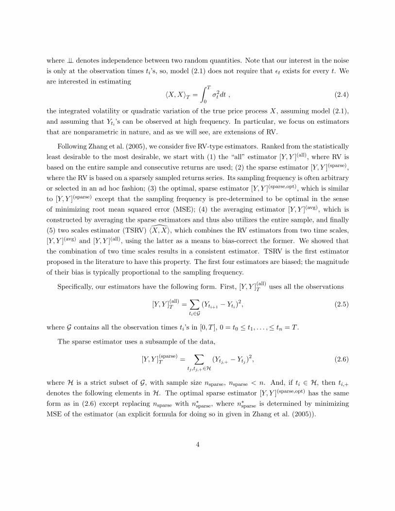
Based on the decomposition (2.9), we have

[Y, Y ](avg)T

L≈ 〈X, X〉T + 2nEε2︸ ︷︷ ︸

bias due to noise

(3.2)

+ [Var([ε, ε](avg)T ) +

8K

[X, X](avg)T Eε2︸ ︷︷ ︸

due to noise

+4T

3n

∫ T

0σ4

t dt︸ ︷︷ ︸due to discretization︸ ︷︷ ︸

]1/2

total variance

Ztotal,

whereVar([ε, ε](avg)

T ) = 4n

KEε4 − 2

KVar(ε2),

and Ztotal is a standard normal term.

The distribution of the optimal averaging estimator [Y, Y ](avg,opt) has the same form as in(3.2) except that we substitute n with the optimal sub-sampling average size n∗. To find n∗, onedetermines K∗ from the bias-variance trade-off in (3.2) and then set n∗ ≈ n/K∗. If one removesthe bias in either [Y, Y ](avg)

T or [Y, Y ](avg,opt)T , it follows from (3.2) that the next term is, again,

asymptotically normal.

3.3. The Failure of Asymptotic Normality

In practice, things are, unfortunately, somewhat more complicated than the story that emergesfrom equations (3.1) and (3.2). The error distributions of the sparse estimators and the averagingestimator can be, in fact, quite far from normal. We provide an illustration of this using simulations.The simulation design is described in Section 5.1 below, but here we give a preview to motivate ourfollowing theoretical development of small sample corrections to these asymptotic distributions.

Figure 1 reports the QQ plots of the standardized distribution of the five estimators before anyEdgeworth correction is applied, as well as the histograms of the estimates. It is clear that thesparse, the sparse-optimal and the averaging estimators are not normally distributed, in particular,they are positively skewed and show some degree of leptokurtosis . On the other hand, the “all”estimator and the TSRV estimator appear to be normally distributed. The apparent normality ofthe “all” estimator is mainly due to the large sample size (one second sampling over 6.5 hours); itis thus fairly irrelevant to talk about its small-sample behavior.

Overall, we conclude from these QQ plots that the small-sample error distribution of the TSRVestimator is close to normality, while the small-sample error distribution of the other estimatorsdeparts from normality. As mentioned in Section 5.1, n is very large in this simulation.

7

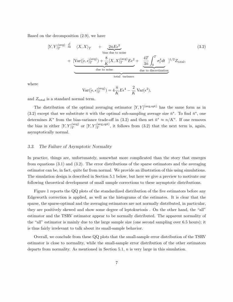
It should be emphasized that bias is not the cause of the non-normality. Apart from TSRV, allthe estimators have substantial bias. This bias, however, does not change the shape of the errordistribution of the estimator, it only changes where the distribution is centered.

4. Edgeworth Expansions for the Distribution of the Estimators

4.1. The Form of the Edgeworth Expansion in Terms of Cumulants

In situations where the normal approximation is only moderately accurate, improved accuracy canbe obtained by appealing to Edgeworth expansions, as follows. Let θ be a quantity to be estimated,such as θ =

∫ T0 σ2

t dt, and let θn be an estimator, say the sparse or average realized volatility, andsuppose that αn is a normalizing constant to that Tn = αn(θn − θ) is asymptotically normal.A better approximation to the density fn of Tn can then be obtained through the Edgeworthexpansion. Typically, second order expansions are sufficient to capture skewness and kurtosis, asfollows:

fn(x) =φ(z)

Var(Tn)1/2

[1 +

16

Cum3(Tn)Var(Tn)3/2

h3(z) +124

Cum4(Tn)Var(Tn)2

h4(z) +172

Cum3(Tn)2

Var(Tn)3h6(z) + ...

](4.1)

where Cumi(Tn) is the i-th order cumulant of Tn, z = (x − E(Tn))/ Var(Tn)1/2, and where theHermite polynomials hi are given by h3(z) = z3 − 3z, h4(z) = z4 − 6z2 + 3, h6(z) = z6 − 15z4 +45z2 − 15. The neglected terms are typically of smaller order in n than the explicit terms. Weshall refer to the explicit terms in (4.1) as the usual Edgeworth form. For broad discussions ofEdgeworth expansions, and definitions of cumulants, see e.g., Chapter XVI of Feller (1971) andChapter 5.3 of McCullagh (1987).

In some cases, Edgeworth expansions can only be found for distribution functions, in which casethe form is obtained by integrating equation (4.1) term by term. In either situation, the Edgeworthapproximations can be turned into expansions for p-values, and to Cornish-Fisher expansions forcritical values; see formula (5.2) below. For more detail, we refer the reader to, e.g., Hall (1992).

Let us now apply this to the problem at hand here. An Edgeworth expansion of the usual form,up to second order, can be found separately for each of the components in (2.9) by first consideringexpansions for n−1/2([ε, ε](all) − 2nEε2) and n−1/2K([ε, ε](avg)

T − 2nEε2). Each of these can then berepresented exactly as a triangular array of martingales. The remaining terms are also, to relevantorder, martingales. Results deriving expansions for martingales can be found in Mykland (1993),Mykland (1995b) and Mykland (1995a). See also Bickel et al. (1986) for n−1/2([ε, ε](all) − 2nEε2).

To implement the expansions, however, one needs the form of the first four cumulants of Tn.

8

We assume that the “size” of the law of ε goes to zero, formally that ε for sample size n is ofthe form τnζ, i.e., Pn(ε/τn ≤ x) = P (ζ ≤ x), where the left hand probability is for sample sizen, and the right hand probability is independent of n. Here, Eζ8 < ∞ and does not depend onsample size, and τn is nonrandom and goes to zero as n → ∞. Note that under our assumption,Var(ε) = O(τ2

n), so the assumption is similar to the small-sigma asymptotics which goes back toKadane (1971). Finally, while in our case this is a way of setting up asymptotics, there is empiricalwork on whether the noise decreases with n; see, in particular, Awartani et al. (2006).

No matter what assumptions are made on the noise (on τn), one should not expect cumulantsin (4.1) to have standard convergence rates. The typical situation for an asymptotically normalstatistic Tn is that the p’th cumulant, p ≥ 2, is of order O(n−(p−2)/2), see, for example, Chapters 2.3-2.4 of Hall (1992), along with Wallace (1958), Bhattacharya and Ghosh (1978), and the discussionin Mykland (2001) and the references therein. While the typical situation does remain in effectfor realized volatility in the no-noise and no-leverage case (which is, after all, a matter simply ofobservations that are independent but non-identically distributed), the picture changes for morecomplex statistics. To see that non-standard rates can occur even in the absence of microstructurenoise, consult (4.28)-(4.29) in Section 4.3.2 below.

An important question which arises in connection with Edgeworth expansions is the comparisonof Cornish-Fisher inversion with bootstrapping. The latter has been developed in the no-noise caseby Goncalves and Meddahi (2009). A comparison of this type is beyond the scope of this paper,but is clearly called for.

4.2. Conditional Cumulants

We start by deriving explicit expressions for the conditional cumulants for [Y, Y ] and [Y, Y ](avg),given the latent process X. All the expressions we give below about [Y, Y ] hold for both [Y, Y ](all)

and [Y, Y ](sparse); in the former case, n remains to be the total sample size in G, while in the lattern is replaced by nsparse. We use a similar notation for [ε, ε] and for [X, X].

4.2.1 Third-Order Conditional Cumulants

Denotec3(n) ∆= Cum3([ε, ε]− 2nEε2), (4.2)

where [ε, ε] =∑n−1

i=0 (εti+1 − εti)2. We have:

9

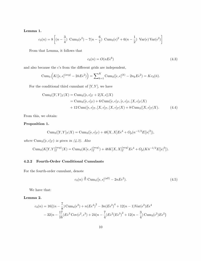
Lemma 1.

c3(n) = 8[(n− 3

4) Cum3(ε2)− 7(n− 6

7) Cum3(ε)2 + 6(n− 1

2) Var(ε) Var(ε2)

]From that Lemma, it follows that

c3(n) = O(nEε6) (4.3)

and also because the ε’s from the different grids are independent,

Cum3

(K([ε, ε](avg) − 2nEε2)

)=∑K

k=1Cum3([ε, ε](k) − 2nkEε2) = Kc3(n).

For the conditional third cumulant of [Y, Y ], we have

Cum3([Y, Y ]T |X) = Cum3([ε, ε]T + 2[X, ε]|X)

= Cum3([ε, ε]T ) + 6 Cum([ε, ε]T , [ε, ε]T , [X, ε]T |X)

+ 12 Cum([ε, ε]T , [X, ε]T , [X, ε]T |X) + 8 Cum3([X, ε]T |X). (4.4)

From this, we obtain:

Proposition 1.

Cum3([Y, Y ]T |X) = Cum3([ε, ε]T ) + 48[X, X]Eε4 + Op(n−1/2E[|ε|3]),

where Cum3([ε, ε]T ) is given in (4.3). Also

Cum3(K[Y, Y ](avg)T |X) = Cum3(K[ε, ε](avg)

T ) + 48K[X, X](avg)T Eε4 + Op(Kn−1/2E[|ε|3]).

4.2.2 Fourth-Order Conditional Cumulants

For the fourth-order cumulant, denote

c4(n) ∆= Cum4([ε, ε](all) − 2nEε2). (4.5)

We have that:

Lemma 2.

c4(n) = 16{(n− 78) Cum4(ε2) + n(Eε4)2 − 3n(Eε2)4 + 12(n− 1)Var(ε2)Eε4

− 32(n− 1716

)Eε3 Cov(ε2, ε3) + 24(n− 74)Eε2(Eε3)2 + 12(n− 3

4) Cum3(ε2)Eε2}

10

Also here,

Cum4

(K([ε, ε](avg) − 2nEε2)

)=∑K

k=1Cum4([ε, ε](k) − 2nkEε2) = Kc4(n).

For the conditional fourth-order cumulant, we know that

Cum4([Y, Y ]|X) = Cum4([ε, ε]T ) + 24 Cum([ε, ε]T , [ε, ε]T , [X, ε]T , [X, ε]T |X)

+ 8 Cum([ε, ε]T , [ε, ε]T , [ε, ε]T , [X, ε]T |X) (4.6)

+ 32 Cum([ε, ε]T , [X, ε]T , [X, ε]T , [X, ε]T |X) + 16 Cum4([X, ε]|X).

Similar argument as in deriving the third cumulant shows that the latter three terms in the righthand side of (4.6) are of order Op(n−1/2E[|ε|5]). Gathering terms of the appropriate order, weobtain:

Proposition 2.

Cum4([Y, Y ]|X) = Cum4([ε, ε]T ) + 24[X, X]T n−1 Cum3([ε, ε]T ) + Op(n−1/2E[|ε|5])

Also, for the average estimator,

Cum4(K[Y, Y ](avg)|X) = Cum4(K[ε, ε](avg)T ) + 24K[X, X](avg)

T

c3(n)n

+ Op(Kn−1/2E[|ε|5])

4.3. Unconditional Cumulants

To get the Edgeworth expansion form as in (4.1), we need unconditional cumulants for the estimator.To pass from conditional to unconditional third cumulants, we will use general formulae for thispurpose (see Brillinger (1969), Speed (1983), and also Chapter 2 in McCullagh (1987)):

Cum3(A) = E[Cum3(A|F)] + 3 Cov[Var(A|F), E(A|F)] + Cum3[E(A|F)]

Cum4(A) = E[Cum4(A|F)] + 4 Cov[Cum3(A|F), E(A|F)] + 3 Var[Var(A|F)]

+ 6 Cum3(Var(A|F), E(A|F), E(A|F)) + Cum4(E(A|F)).

In what follows, we apply these formulae to derive the unconditional cumulants for our estimators.The main development (after formula 4.8) will be for the case where there is no leverage effect. Itshould be noted that there are (other) cases, such as Bollerslev and Zhou (2002) and Corradi andDistaso (2006), involving leverage effect where (non-mixed) asymptotic normality holds. In suchcase, unconditional Edgeworth expansions may also be applicable.

11

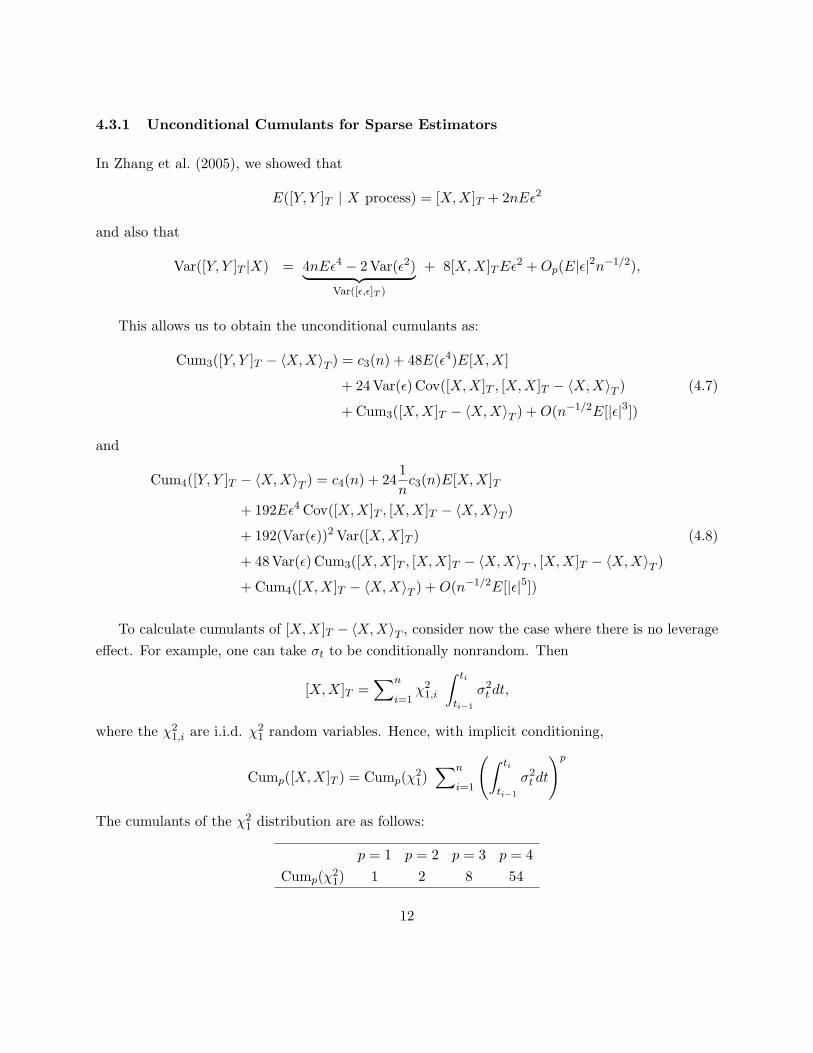
4.3.1 Unconditional Cumulants for Sparse Estimators

In Zhang et al. (2005), we showed that

E([Y, Y ]T | X process) = [X, X]T + 2nEε2

and also that

Var([Y, Y ]T |X) = 4nEε4 − 2 Var(ε2)︸ ︷︷ ︸Var([ε,ε]T )

+ 8[X, X]T Eε2 + Op(E|ε|2n−1/2),

This allows us to obtain the unconditional cumulants as:

Cum3([Y, Y ]T − 〈X, X〉T ) = c3(n) + 48E(ε4)E[X, X]

+ 24 Var(ε) Cov([X, X]T , [X, X]T − 〈X, X〉T ) (4.7)

+ Cum3([X, X]T − 〈X, X〉T ) + O(n−1/2E[|ε|3])

and

Cum4([Y, Y ]T − 〈X, X〉T ) = c4(n) + 241n

c3(n)E[X, X]T

+ 192Eε4 Cov([X, X]T , [X, X]T − 〈X, X〉T )

+ 192(Var(ε))2 Var([X, X]T ) (4.8)

+ 48 Var(ε) Cum3([X, X]T , [X, X]T − 〈X, X〉T , [X, X]T − 〈X, X〉T )

+ Cum4([X, X]T − 〈X, X〉T ) + O(n−1/2E[|ε|5])

To calculate cumulants of [X, X]T − 〈X, X〉T , consider now the case where there is no leverageeffect. For example, one can take σt to be conditionally nonrandom. Then

[X, X]T =∑n

i=1χ2

1,i

∫ ti

ti−1

σ2t dt,

where the χ21,i are i.i.d. χ2

1 random variables. Hence, with implicit conditioning,

Cump([X, X]T ) = Cump(χ21)∑n

i=1

(∫ ti

ti−1

σ2t dt

)p

The cumulants of the χ21 distribution are as follows:

p = 1 p = 2 p = 3 p = 4Cump(χ2

1) 1 2 8 54

12

When the sampling points are equidistant, one then obtains the approximation

Cump([X, X]T ) = Cump(χ21)(

T

n

)p−1 ∫ T

0σ2p

t dt + O(n12−p)

under the assumption that σ2t is an Ito process (often called a Brownian semimartingale). Hence,

we have:

Proposition 3. In the case where there is no leverage effect, conditionally on the path of σ2t ,

Cum3([Y, Y ]T − 〈X, X〉T ) = c3(n) + 48E(ε4)∫ T

0σ2

t dt

+ 48 Var(ε)n−1T

∫ T

0σ4

t dt + 8n−2T 2

∫ T

0σ6

t dt (4.9)

+ O(n−3/2E[ε2]) + O(n−1/2E[|ε|3]) + O(n−5/2)

Similarly for the fourth cumulant

Cum4([Y, Y ]T − 〈X, X〉T ) = c4(n) + 24n−1c3(n)∫ T

0σ2

t dt

+ 384(Eε4 + Var(ε)2)n−1T

∫ T

0σ4

t dt (4.10)

+ 384 Var(ε)n−2T 2

∫ T

0σ6

t dt + 54n−3T 3

∫ T

0σ8

t dt

+ O(n−1/2E[|ε|5]) + O(n−3/2E[ε4]) + O(n−5/2E[ε2]) + O(n−7/2)

If one chooses ε = op(n−1/2) (i.e., τn = o(n−1/2)), then all the explicit terms in (4.9) and (4.10)are non-negligible. In this case, the error term in equation (4.9) is of order O(n−1/2E[|ε|3]) +O(n−5/2), while that in equation (4.10) is of order O(n−1/2E[|ε|5]) + O(n−7/2). In the case ofoptimal-sparse estimator, it is shown in Zhang et al. (2005) (Section 2.3) that the optimal samplingfrequency leads to ε = Op(n−3/4), in particular ε = op(n−1/2).

For the special case of equidistant sampling times, the optimal sampling size is (ibid, equation(31), p. 1399)

n∗sparse =(

T

4(Eε2)2

∫ T

0σ4

t dt

)1/3

. (4.11)

Also, in this case, it is easy to see that the error terms in equations (4.9) and (4.10) are, respectively,O(n−1/2E[|ε|3]) and O(n−1/2E[|ε|5]). Plug (4.11) into (4.9) and (4.10) for the choice of n, and it

13

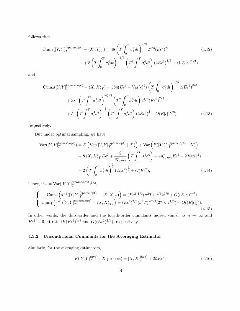
follows that

Cum3([Y, Y ](sparse,opt)T − 〈X, X〉T ) = 48

(T

∫ T

0σ4

t dt

)2/3

22/3(Eε2)5/3 (4.12)

+ 8(

T

∫ T

0σ4

t dt

)−2/3(T 2

∫ T

0σ6

t dt

)(2Eε2)4/3 + O(E|ε|11/3)

and

Cum4([Y, Y ](sparse,opt)T − 〈X, X〉T ) = 384(Eε4 + Var(ε)2)

(T

∫ T

0σ4

t dt

)2/3

(2Eε2)2/3

+ 384(

T

∫ T

0σ4

t dt

)−2/3(T 2

∫ T

0σ6

t dt

)24/3(Eε2)7/3

+ 54(

T

∫ T

0σ4

t dt

)−1(T 3

∫ T

0σ8

t dt

)(2Eε2)2 + O(E|ε|17/3) (4.13)

respectively.

But under optimal sampling, we have

Var([Y, Y ](sparse,opt)T ) = E

(Var([Y, Y ](sparse,opt)

T | X))

+ Var(E([Y, Y ](sparse,opt)

T | X))

= 8 〈X, X〉T Eε2 +2

n∗sparse

(T

∫ T

0σ4

t dt

)+ 4n∗sparseEε4 − 2 Var(ε2)

= 2(

T

∫ T

0σ4

t dt

) 23

(2Eε2)23 + O(Eε2), (4.14)

hence, if s = Var([Y, Y ](sparse,opt)T )1/2, Cum3

(s−1([Y, Y ](sparse,opt)

T − 〈X, X〉T ))

= (Eε2)1/3(σ2T )−1/325/6 + O((E|ε|)4/3)

Cum4

(s−1([Y, Y ](sparse,opt)

T − 〈X, X〉T ))

= (Eε2)2/3(σ2T )−2/3(27× 21/3) + O((E|ε|)2).(4.15)

In other words, the third-order and the fourth-order cumulants indeed vanish as n → ∞ andEε2 → 0, at rate O((Eε2)1/3 and O((Eε2)2/3), respectively.

4.3.2 Unconditional Cumulants for the Averaging Estimator

Similarly, for the averaging estimators,

E([Y, Y ](avg)T | X process) = [X, X](avg)

T + 2nEε2, (4.16)

14

Var([Y, Y ](avg)T |X) = Var([ε, ε](avg)

T ) +8K

[X, X](avg)T Eε2 + Op(E[|ε|2(nK)−1/2]), (4.17)

withVar([ε, ε](avg)

T ) = 4n

KEε4 − 2

KVar(ε2). (4.18)

Also, from Zhang et al. (2005), for nonrandom σt, we have that

Var([X, X](avg)T ) =

K

n

43T

∫ T

0σ4

t dt + o

(K

n

). (4.19)

Invoking the general relations between the conditional and the unconditional cumulants givenabove, we get the unconditional cumulants for the average estimator:

Cum3([Y, Y ](avg)T − 〈X, X〉T ) =

1K2

c3(n) + 481

K2E(ε4)E[X, X](avg)

T

+ 241K

Var(ε) Cov([X, X](avg)T , [X, X](avg)

T − 〈X, X〉T ) (4.20)

+ Cum3([X, X](avg)T − 〈X, X〉T ) + O(K−2n−1/2E[|ε|3])

and

Cum4([Y, Y ](avg)T − 〈X, X〉T ) =

1K3

c4(n) + 241

K3

c3(n)n

E[X, X](avg)T

+ 1921

K2Eε4 Cov([X, X](avg)

T , [X, X](avg)T − 〈X, X〉T )

+ 1921

K2(Var(ε))2 Var([X, X](avg)

T ) (4.21)

+ 481K

Var(ε) Cum3([X, X](avg)T , [X, X](avg)

T − 〈X, X〉T , [X, X](avg)T − 〈X, X〉T )

+ Cum4([X, X](avg)T − 〈X, X〉T ) + O(K−3n−1/2E[|ε|5])

To calculate cumulants of [X, X](avg)T −〈X, X〉T for the case where there is no leverage effect, we

shall use the following proposition, which has some independent interest. We suppose that Dt is aprocess, Dt =

∫ t0 ZsdWs. We also assume that (1) Zs has mean zero, (2) is adapted to the filtration

generated by Wt, and also (3) jointly Gaussian with Wt. The first two of these assumptions imply,by the martingale representation theorem, that one can write

Zs =∫ s

0f(s, u)dWu, (4.22)

the third assumption yields that this f(s, u) is nonrandom, with representation Cov(Zs,Wt) =∫ t0 f(s, u)du for 0 ≤ t ≤ s ≤ T .

15

Obviously, Var(DT ) =∫ T0 E(Z2

s )ds =∫ T0

∫ s0 f(s, u)2duds. The following result provides the

third and fourth cumulants of DT . Note that for u ≤ s

Cov(Zs, Zu) =∫ u

0f(s, t)f(u, t)dt. (4.23)

Proposition 4. Under the assumptions above,

Cum3(DT ) = 6∫ T

0ds

∫ s

0Cov(Zs, Zu)f(s, u)du = 6

∫ T

0ds

∫ s

0du

∫ u

0f(s, u)f(s, t)f(u, t)dt (4.24)

Cum4(DT ) = −12∫ T

0ds

∫ s

0dt

(∫ t

0f(s, u)f(t, u)du

)2

+ 24∫ T

0ds

∫ s

0dx

∫ x

0du

∫ u

0dt (f(x, u)f(x, t)f(s, u)f(s, t) (4.25)

+ f(x, u)f(u, t)f(s, x)f(s, t) + f(x, t)f(u, t)f(s, x)f(s, u))

The proof is in the appendix. Note that it is possible to derive similar results in the multivariatecase. See, for example, equation (E.3) in the appendix. For the application to our case, note thatwhen σt is (conditionally or unconditionally) nonrandom, DT = [X, X](avg)

T − 〈X, X〉T is on theform discussed above, with

f(s, u) = σsσu2K

(K −#tj between u and s)+ . (4.26)

This provides a general form of the low order cumulants of [X, X](avg)T . In the equidistant case, one

can, in the equations above, to first order make the approximation

f(s, u) ≈ 2σsσu

(1− s− u

K∆t

)+

. (4.27)

This yields, from Proposition 4,

Cum3([X, X](avg)T ) = 48

(K

n

)2

T 2

∫ T

0σ6

t dt

∫ 1

0dy

∫ 1

0dx (1− y)(1− x)(1− (x + y))+

= 48(

K

n

)2

T 2

∫ T

0σ6

t dt

∫ 1

0dz

∫ 1

1−zdv zv(z + v − 1) + o

((K

n

)2)

=4410

(K

n

)2

T 2

∫ T

0σ6

t dt + o

((K

n

)2)

(4.28)

16

and

Cum4([X, X](avg)T ) =

(K

n

)3

T 3

∫ T

0σ8

t dt

{−192

∫ 1

0dy

(∫ 1

0(1− (x + y))+(1− x)dx

)2

+384∫ 1

0dz

∫ 1

0dy

∫ 1

0dw[(1− y)+(1− (y + w))+(1− (y + z))+(1− (w + y + z))+

+ (1− y)+(1− w)+(1− z)+(1− (w + y + z))+

+(1− (w + y))+(1− w)+(1− z)+(1− (y + z))+]}

+ o

((K

n

)3)

=1888105

(K

n

)3

T 3

∫ T

0σ8

t dt + o

((K

n

)3)

(4.29)

Thus, (4.20) and (4.21) lead to the following results:

Proposition 5. In the case where there is no leverage effect, conditionally on the path of the σ2t ,

Cum3([Y, Y ](avg)T − 〈X, X〉T ) =1

K28{

(n− 34) Cum3(ε2)− 7(n− 6

7) Cum3(ε)2

+ 6(n− 12) Var(ε) Var(ε2)

}+ 48

1K2

E(ε4)∫ T

0σ2

t dt +963

1n

E(ε2)T∫ T

0σ4

t dt (4.30)

+4410

(K

n

)2

T 2

∫ T

0σ6

t dt + smaller terms

Cum4([Y, Y ](avg)T − 〈X, X〉T ) = 16n

K3{Cum4(ε2) + (Eε4)2 − 3(Eε2)4 + 12Var(ε2)Eε4

− 32Eε3 Cov(ε2, ε3) + 24Eε2(Eε3)2 + 12 Cum3(ε2)Eε2}+ O(1

K3E|ε|8)

+ 1921

K3

{Cum3(ε2)− 7 Cum3(ε)2 + 6 Var(ε) Var(ε2)

}∫ T

0σ2

t dt + O(1

nK2E|ε|6)

+ 2561

nK

(Eε4 + (Var(ε))2

)T

∫ T

0σ4

t dt + o(1

nKE|ε|4) (4.31)

+211210

K

n2Var(ε)T 2

∫ T

0σ6

t dt + o(K

n2E|ε|2)

+1888105

(K

n

)3

T 3

∫ T

0σ8

t dt + o((

K

n

)3

) + smaller terms

Also, the optimal average subsampling size is,

n∗ =(

T

6(Eε2)2

∫ T

0σ4

t dt

)1/3

.

17

The unconditional cumulants of the averaging estimator under the optimal sampling are Cum3([Y, Y ](avg,opt)T − 〈X, X〉T ) = 22

5

(Kn

)2T 2∫ T0 σ6

t dt + o((

Kn

)2),

Cum4([Y, Y ](avg,opt)T − 〈X, X〉T ) = 1888

105

(Kn

)3T 3∫ T0 σ8

t dt + o((

Kn

)3).

Also, the unconditional variance of the averaging estimator, under the optimal sampling, is

Var([Y, Y ](avg,opt)T ) =

8K

Eε2∫ T

0σ2

t dt + 4n∗

KEε4 − 2

KVar(ε2)︸ ︷︷ ︸

=E“Var([Y,Y ]

(avg,opt)T | X)

”+

K

n∗43T

∫ T

0σ4

t dt + o(K

n∗)︸ ︷︷ ︸

=Var“E([Y,Y ]

(avg,opt)T | X)

”(4.32)

=436

13 (Eε2)

23

(T

∫ T

0σ4

t dt

) 23

+ o(E|ε|4/3)

hence, if we write s = Var([Y, Y ](avg,opt)T )1/2, we have that Cum3

(s−1([Y, Y ](avg,opt)

T − 〈X, X〉T ))

= (Eε2)1/3(σ2T )−1/3(115 × 2−11/6 × 35/3) + O((Eε2)2/3),

Cum4

(s−1([Y, Y ](avg,opt)

T − 〈X, X〉T ))

= (Eε2)2/3(σ2T )−2/361/3 35435 + O((Eε2))

(4.33)as n →∞ and Eε2 → 0.

It is interesting to note that the averaging estimator is no closer to normal than the sparseestimator. In fact, by comparing the expression for the third cumulants in (4.15) and (4.33), wefind an increase in skewness of

Cum3

(s−1([Y, Y ](avg,opt)

T − 〈X, X〉T ))

Cum3

(s−1([Y, Y ](sparse,opt)

T − 〈X, X〉T )) =

(Eε2)1/3(σ2T )−1/3(115 × 2−11/6 × 35/3) + O((E|ε|)4/3)

(Eε2)1/3(σ2T )−1/325/6 + O((E|ε|)4/3)

=115× 2−8/3 × 35/3 + O((E|ε|)2/3) ≈ 216%. (4.34)

This number does not fully reflect the change is skewness, since it is only a first order term andthe higher order terms also matter, cf. our simulations in the next section. (The simulations usethe most precise formulas above, see Table 1 for details.)

18

4.4. Cumulants for the TSRV Estimator

The same methods can be used to find cumulants for the two scales realized volatility (TSRV)estimator, 〈X, X〉T . Since the distribution of TSRV is well approximated by its asymptotic normaldistribution, we only sketch the results. When ε goes to zero sufficiently fast, the dominating termin the third and fourth unconditional cumulants for TSRV are, symbolically, the same as for theaverage volatility, namely Cum3(〈X, X〉T − 〈X, X〉T ) = 22

5

(Kn

)2T 2∫ T0 σ6

t dt + o((

Kn

)2),

Cum4(〈X, X〉T − 〈X, X〉T ) = 1888105

(Kn

)3T 3∫ T0 σ8

t dt + o((

Kn

)3).

(4.35)

However, the value of K is quite different for TSRV than for the averaging volatility estimator. Itis shown in Section 4 of Zhang et al. (2005) that for TSRV, the optimal choice of K is given by

K =(

T

12(Eε2)2

∫ T

0σ4

t dt

)−1/3

n2/3. (4.36)

As is seen from Table 1, this choice of K gives radically different distributional properties than thosefor the average volatility. This is consistent with the behavior in simulation. Thus, as predicted,the normal approximation works well in this case.

5. Simulation Results Incorporating the Edgeworth Correction

In this paper, we have discussed five estimators to deal with the microstructure noise in real-ized volatility. The five estimators, including [Y, Y ](all)T , [Y, Y ](sparse)

T , [Y, Y ](sparse,opt)T , [Y, Y ](avg)

T ,〈X, X〉T , are defined in Section 2. In this section, we focus on the case where the sampling pointsare regularly allocated. We first examine the empirical distributions of the five approaches in sim-ulation. We then apply the the Edgeworth corrections as developed in Section 4, and compare thesample performance to those predicted by the asymptotic theory.

We simulate M = 50, 000 sample paths from the standard Heston stochastic model

dXt =(µ− σ2

t /2)dt + σtdBt

dσ2t = κ(α− σ2

t )dt + γσtdWt

at a time interval ∆t = 1 second, with parameter values µ = 0.05, α = 0.04, κ = 5, γ = 0.05 andρ = d 〈B,W 〉t /dt = −0.5. As for the market microstructure noise ε, we assume that it is Gaussianwith mean zero and standard deviation

(Eε2

)1/2 = 0.0005 (i.e., only 0.05% of the value of the asset

19

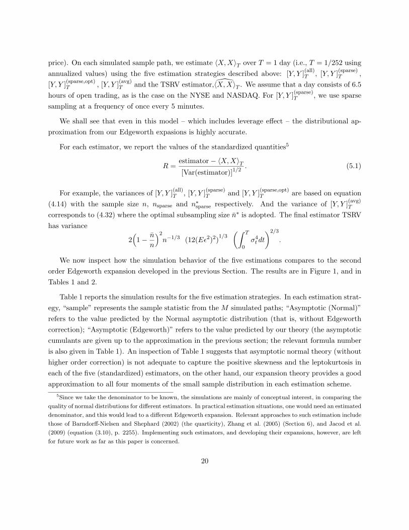
price). On each simulated sample path, we estimate 〈X, X〉T over T = 1 day (i.e., T = 1/252 usingannualized values) using the five estimation strategies described above: [Y, Y ](all)T , [Y, Y ](sparse)

T ,

[Y, Y ](sparse,opt)T , [Y, Y ](avg)

T and the TSRV estimator,〈X, X〉T . We assume that a day consists of 6.5hours of open trading, as is the case on the NYSE and NASDAQ. For [Y, Y ](sparse)

T , we use sparsesampling at a frequency of once every 5 minutes.

We shall see that even in this model – which includes leverage effect – the distributional ap-proximation from our Edgeworth expasions is highly accurate.

For each estimator, we report the values of the standardized quantities5

R =estimator− 〈X, X〉T[Var(estimator)]1/2

. (5.1)

For example, the variances of [Y, Y ](all)T , [Y, Y ](sparse)T and [Y, Y ](sparse,opt)

T are based on equation(4.14) with the sample size n, nsparse and n∗sparse respectively. And the variance of [Y, Y ](avg)

T

corresponds to (4.32) where the optimal subsampling size n∗ is adopted. The final estimator TSRVhas variance

2(1− n

n

)2

n−1/3 (12(Eε2)2)1/3(∫ T

0σ4

t dt

)2/3

.

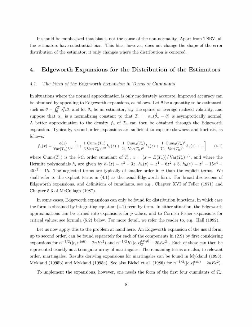
We now inspect how the simulation behavior of the five estimations compares to the secondorder Edgeworth expansion developed in the previous Section. The results are in Figure 1, and inTables 1 and 2.

Table 1 reports the simulation results for the five estimation strategies. In each estimation strat-egy, “sample” represents the sample statistic from the M simulated paths; “Asymptotic (Normal)”refers to the value predicted by the Normal asymptotic distribution (that is, without Edgeworthcorrection); “Asymptotic (Edgeworth)” refers to the value predicted by our theory (the asymptoticcumulants are given up to the approximation in the previous section; the relevant formula numberis also given in Table 1). An inspection of Table 1 suggests that asymptotic normal theory (withouthigher order correction) is not adequate to capture the positive skewness and the leptokurtosis ineach of the five (standardized) estimators, on the other hand, our expansion theory provides a goodapproximation to all four moments of the small sample distribution in each estimation scheme.

5Since we take the denominator to be known, the simulations are mainly of conceptual interest, in comparing the

quality of normal distributions for different estimators. In practical estimation situations, one would need an estimated

denominator, and this would lead to a different Edgeworth expansion. Relevant approaches to such estimation include

those of Barndorff-Nielsen and Shephard (2002) (the quarticity), Zhang et al. (2005) (Section 6), and Jacod et al.

(2009) (equation (3.10), p. 2255). Implementing such estimators, and developing their expansions, however, are left

for future work as far as this paper is concerned.

20

In Table 2, we report coverage probabilities computed as follows: for asymptotically standardnormal Tn, let zα be the upper 1− α quantile (so Φ(zα) = 1− α) and set

wα,n = zα +16

Cum3(Tn)(z2α − 1) +

124

Cum4(Tn)(z3α − 3zα) +

172

Cum3(Tn)2(−4z3α + 10zα). (5.2)

The second order Cornish-Fisher corrected interval has actual coverage probability P (Tn ≤ wα,n)(which should be close to 1 − α, but not exactly equal to it). The normal approximation gives acoverage probability P (Tn ≤ zα). We report these values for a = 0.10, 0.05 and 0.01. The resultsshow that the Edgeworth-based coverage probabilities provide very accurate approximations to thesample ones, compared to the Normal-based coverage probabilities.

Figure 1 confirms that the sample distributions of all five estimators conform to our Edgeworthexpansion. The nonlinearity in the QQ plots (left panels) reminds us that normal asymptotic theorywithout Edgeworth expansion fails to describe the sample behaviors of [Y, Y ](sparse)

T , [Y, Y ](sparse,opt)T

and [Y, Y ](avg)T . The histograms in the right panels display the standardized distribution of the five

estimators obtained from simulation results, and the superimposed solid curve corresponds to theasymptotic distribution predicted by our Edgeworth expansion. The dashed curve represents theuncorrected N(0, 1) distribution. By comparing the deviation between the dashed and solid curves,we can see how Edgeworth correction helps to capture the right skewness and leptokurtosis in thesample distribution of the (standardized) estimators.

6. Conclusions

We have developed and given formulas for Edgeworth expansions of several type of realized volatilityestimators. Apart from the practical interest of having access to such expansions, there is animportant conceptual finding. That is, a better expansion is obtained by using an asymptoticswhere the noise level goes to zero when the number of observations goes to infinity. Another lessonis that the asymptotic normal distribution is a more accurate approximation for the two scalesrealized volatility (TSRV) than for the subsampled estimators, whose distributions definitely needto be Edgeworth-corrected in small samples.

In the process of developing the expansions, we also developed a general device for computingcumulants of the integrals of Gaussian processes with respect to Brownian motion (Proposition4), and this result should have applications to other situations. The proposition is only stated forthe third and fourth cumulant, but the same technology can potentially be used for higher ordercumulants.

21

References

Aıt-Sahalia, Y., Mykland, P. A., Zhang, L., 2005. How often to sample a continuous-time processin the presence of market microstructure noise. Review of Financial Studies 18, 351–416.

Andersen, T. G., Bollerslev, T., Diebold, F. X., Ebens, H., 2001a. The distribution of realized stockreturn volatility. Journal of Financial Economics 61, 43–76.

Andersen, T. G., Bollerslev, T., Diebold, F. X., Labys, P., 2001b. The distribution of realizedexchange rate volatility. Journal of the American Statistical Association 96, 42–55.

Awartani, B., Corradi, V., Distaso, W., 2006. Testing and modelling microstructure effects with anapplication to the Dow Jones industrial average, working Paper, University of Warwick.

Bandi, F. M., Russell, J. R., 2008. Microstructure noise, realized volatility and optimal sampling.Review of Economic Studies 75, 339–369.

Barndorff-Nielsen, O. E., Hansen, P. R., Lunde, A., Shephard, N., 2008. Designing realized kernelsto measure ex-post variation of equity prices in the presence of noise. Econometrica 76, 1481–1536.

Barndorff-Nielsen, O. E., Hansen, P. R., Lunde, A., Shephard, N., 2009. Subsampling realisedkernels. Journal of Econometrics, forthcoming .

Barndorff-Nielsen, O. E., Shephard, N., 2002. Econometric analysis of realized volatility and its usein estimating stochastic volatility models. Journal of the Royal Statistical Society, B 64, 253–280.

Barndorff-Nielsen, O. E., Shephard, N., 2005. How accurate is the asymptotic approximation tothe distribution of realized variance? In: Andrews, D. W., Stock, J. H. (Eds.), Identificationand Inference for Econometric Models. A Festschrift in Honour of T.J. Rothenberg. CambridgeUniversity Press, Cambridge, UK, pp. 306–311.

Bhattacharya, R. N., Ghosh, J., 1978. On the validity of the formal Edgeworth expansion. Annalsof Statistics 6, 434–451.

Bickel, P. J., Gotze, F., van Zwet, W. R., 1986. The Edgeworth expansion for u-statistics of degreetwo. The Annals of Statistics 14, 1463–1484.

Bollerslev, T., Zhou, H., 2002. Estimating stochastic volatility diffusions using conditional momentsof integrated volatility. Journal of Econometrics 109, 33–65.

Brillinger, D. R., 1969. The calculation of cumulants via conditioning. Annals of the Institute ofStatistical Mathematics 21, 215–218.

Chan, N. H., Wei, C. Z., 1987. Asymptotic inference for nearly nonstationary AR(1) processes.Annals of Statistics 15, 1050–1063.

22

Corradi, V., Distaso, W., 2006. Semiparametric comparison of stochastic volatility models viarealized measures. Review of Economic Studies 73, 635–667.

Dacorogna, M. M., Gencay, R., Muller, U., Olsen, R. B., Pictet, O. V., 2001. An Introduction toHigh-Frequency Finance. Academic Press, San Diego.

Delattre, S., Jacod, J., 1997. A central limit theorem for normalized functions of the increments ofa diffusion process, in the presence of round-off errors. Bernoulli 3, 1–28.

Feller, W., 1971. An Introduction to Probability Theory and Its Applications, Volume 2. JohnWiley and Sons, New York.

Gloter, A., Jacod, J., 2001. Diffusions with measurement errors. II - optimal estimators. ESAIM 5,243–260.

Goncalves, S., Meddahi, N., 2008. Edgeworth corrections for realized volatility. Econometric Re-views 27, 139–162.

Goncalves, S., Meddahi, N., 2009. Bootstrapping realized volatility. Econometrica 77, 283–306.

Hall, P., 1992. The bootstrap and Edgeworth expansion. Springer, New York.

Hansen, P. R., Lunde, A., 2006. Realized variance and market microstructure noise. Journal ofBusiness and Economic Statistics 24, 127–218.

Jacod, J., 1994. Limit of random measures associated with the increments of a Brownian semi-martingale. Tech. rep., Universite de Paris VI.

Jacod, J., Li, Y., Mykland, P. A., Podolskij, M., Vetter, M., 2009. Microstructure noise in thecontinuous case: The pre-averaging approach. Stochastic Processes and Their Applications 119,2249–2276.

Jacod, J., Protter, P., 1998. Asymptotic error distributions for the euler method for stochasticdifferential equations. Annals of Probability 26, 267–307.

Kadane, J. B., 1971. Comparison of k-class estimators when the disturbances are small. Economet-rica 39, 723–737.

Lieberman, O., Phillips, P. C., 2006. Refined inference on long memory in realized volatility, CowlesFoundation Discussion Paper No. 1549.

McCullagh, P., 1987. Tensor Methods in Statistics. Chapman and Hall, London, U.K.

Meddahi, N., 2002. A theoretical comparison between integrated and realized volatility. Journal ofApplied Econometrics 17, 479–508.

Mykland, P. A., 1993. Asymptotic expansions for martingales. Annals of Probability 21, 800–818.

Mykland, P. A., 1994. Bartlett type identities for martingales. Annals of Statistics 22, 21–38.

23

Mykland, P. A., 1995a. Embedding and asymptotic expansions for martingales. Probability Theoryand Related Fields 103, 475–492.

Mykland, P. A., 1995b. Martingale expansions and second order inference. Annals of Statistics 23,707–731.

Mykland, P. A., 2001. Likelihood computations without Bartlett identities. Bernoulli 7, 473–485.

Mykland, P. A., Zhang, L., 2006. ANOVA for diffusions and Ito processes. Annals of Statistics 34,1931–1963.

Podolskij, M., Vetter, M., 2009. Estimation of volatility functionals in the simultaneous presenceof microstructure noise and jumps. Bernoulli, forthcoming .

Speed, T. P., 1983. Cumulants and partition lattices. The Australian Journal of Statistics 25,378–388.

Wallace, D. L., 1958. Asymptotic approximations to distributions. Annals of Mathematical Statis-tics 29, 635–654.

Zhang, L., 2001. From martingales to ANOVA: Implied and realized volatility. Ph.D. thesis, TheUniversity of Chicago, Department of Statistics.

Zhang, L., 2006. Efficient estimation of stochastic volatility using noisy observations: A multi-scaleapproach. Bernoulli 12, 1019–1043.

Zhang, L., Mykland, P. A., Aıt-Sahalia, Y., 2005. A tale of two time scales: Determining integratedvolatility with noisy high-frequency data. Journal of the American Statistical Association 100,1394–1411.

Zhou, B., 1996. High-frequency data and volatility in foreign-exchange rates. Journal of Business& Economic Statistics 14, 45–52.

Zhou, B., 1998. F-consistency, de-volatization and normalization of high frequency financial data.In: Dunis, C. L., Zhou, B. (Eds.), Nonlinear Modelling of High Frequency Financial Time Series.John Wiley Sons Ltd., New York, pp. 109–123.

Zumbach, G., Dacorogna, M., Olsen, J., Olsen, R., 1999. Introducing a scale of market shocks.Tech. rep., Olsen & Associates.

24

Appendix: Proofs

A. Proof of Lemma 1

Let ai be defined by

ai ={

1 if 1 ≤ i ≤ n− 112 if i = 0, n

(A.1)

We can then write

c3(n) = Cum3(2∑n

i=0ai(ε2ti − Eε2)− 2

∑n−1

i=0εtiεti+1),

= 8[Cum3(∑n

i=0aiε

2ti)− Cum3(

∑n−1

i=0εtiεti+1)

− 3 Cum(∑n

i=0aiε

2ti ,∑n

j=0ajε

2tj ,∑n−1

k=0εtkεtk+1

)

+ 3 Cum(∑n

i=0aiε

2ti ,∑n−1

j=0εtj εtj+1 ,

∑n−1

k=0εtkεtk+1

)] (A.2)

where

Cum(∑n

i=0aiε

2ti ,∑n

j=0ajε

2tj ,∑n−1

k=0εtkεtk+1

) = 2∑n−1

k=0akak+1 Cum(ε2tk , ε2tk+1

, εtkεtk+1)

= 2(n− 1)(Eε3)2 (A.3)

since∑n−1

k=0 akak+1 = n − 1, and the summation is non-zero only when (i = k, j = k + 1) or(i = k + 1, j = k). Also,

Cum(∑n

i=0aiε

2ti ,∑n−1

j=0εtj εtj+1 ,

∑n−1

k=0εtkεtk+1

) = 2∑n−1

j=0aj Cum(ε2tj , εtj εtj+1 , εtj εtj+1)

= 2(n− 12)(Eε2) Var(ε2) (A.4)

since∑n−1

j=0 aj = n− 12 , and the summation is non-zero only when j = k = (i, or i−1). And finally,

Cum(∑n−1

i=0εtiεti+1 ,

∑n−1

j=0εtj εtj+1 ,

∑n−1

k=0εtkεtk+1

) =∑n−1

i=0Cum3(εtiεti+1) = n(Eε3)2, (A.5)

Cum(∑n

i=0aiε

2ti ,∑n

j=0ajε

2tj ,∑n

k=0akε

2tk

) =∑n

i=0a3

i Cum3(ε2ti) = (n− 34) Cum3(ε2), (A.6)

with∑n

i=0 a3i = n− 3

4 . Inserting (A.3)-(A.6) in (A.2) yields (4.3).

B. Proof of Proposition 1

To proceed, define

bi =

∆Xti−1 −∆Xti if 1 ≤ i ≤ n− 1∆Xtn−1 if i = n−∆Xt0 if i = 0

(B.1)

25

Note that [X, ε]T =∑n

i=0 biεti . Then it follows that

Cum([ε, ε]T , [ε, ε]T , [X, ε]T |X) =∑n

i=0bi Cum([ε, ε]T , [ε, ε]T , εti)

= (b0 + bn)[2Eε2Eε3 − 3Eε5] = Op(n−1/2E[|ε|5])

because Cum([ε, ε]T , [ε, ε]T , εti) = Cum([ε, ε]T , [ε, ε]T , εt1), for i = 1, · · · , n − 1. Also, recalling thedefinition of ai in (A.1)

Cum([ε, ε]T , [X, ε]T ,[X, ε]T |X) = Cum(2∑n

i=0aiε

2ti ,∑n

j=0bjεtj ,

∑n

k=0bkεtk |X)

− Cum(2∑n−1

i=0εtiεti+1 ,

∑n

j=0bjεtj ,

∑n

k=0bkεtk |X)

= 2∑n

i=0aib

2i Var(ε2)− 4

∑n−1

i=0bibi+1(Var(ε))2 (B.2)

= 4[X, X]T Eε4 + Op(n−1/2E[ε4])

Finally,

Cum3([X, ε]T |X) =∑n

i=0b3i Cum3(ε)

= Eε3[−3∑n−1

i=1(∆Xti−1)

2(∆Xti) + 3∑n−1

i=1(∆Xti−1)(∆Xti)

2] (B.3)

= Op(n−1/2E[|ε|3])

Gathering the terms above together, one now obtains the first part of Proposition 1. The secondpart of the result is then obvious.

C. Proof of Lemma 2

We have that:

Cum(∑n

i=0aiε

2ti ,∑n−1

j=0εtj εtj+1 ,

∑n−1

k=0εtkεtk+1

,∑n−1

l=0εtlεtl+1

)

=∑n

i=0

∑n−1

j=k=0ai[1{l=j}1{i=j,or j+1} +

(32

)(1{l=j+1,i=j+2} + 1{l=i=j−1})]

× Cum(ε2ti , εtj εtj+1 , εtkεtk+1, εtlεtl+1

) (C.1)

= 2(n− 12)Eε3 Cov(ε2, ε3) + 6(n− 3

2)(Eε3)2Eε2

Cum(∑n

i=0aiε

2ti ,∑n

j=0ajε

2tj ,∑n−1

k=0εtkεtk+1

,∑n−1

l=0εtlεtl+1

)

=∑n

i=0

∑n

j=0

∑n−1

k=0

∑n−1

l=0aiaj

[1{i=j,k=l,i=(k+1 or k)} + 1{l=k−1,(i,j)=(k+1,k−1)[2]}

+ 1{l=k+1,(i,j)=(k,k+2)[2]} + 1{k=l,(i,j)=(k,k+1)[2]}]

(C.2)

= 2(n− 34) Cum3(ε2)Eε2 + 4(n− 2)(Eε3)2Eε2 + 2(n− 1)(Var(ε2))2

26

where the notation (i, j) = (k + 1, k − 1)[2] means that (i = k + 1, j = k − 1), or (j = k + 1, i =k − 1). The last equation above holds because

∑ni=1 a2

i = n − 3/4,∑n−1

i=1 ai−1ai+1 = n − 2, and∑n−1i=0 aiai+1 = n− 1. Next:

Cum(∑n

i=0aiε

2ti ,∑n

j=0ajε

2tj ,∑n

k=0akε

2tk

,∑n−1

l=0εtlεtl+1

)

=∑n

i=0

∑n

j=0

∑n−1

k=0

∑n−1

l=0aiajak

(32

)[1{i=j=l,k=l+1} + 1{i=j=l+1,k=l}]

× Cum(ε2ti , ε2tj , ε

2tk

, εtlεtl+1) (C.3)

= 6∑n−1

i=0a2

i ai+1 Cum(ε2, ε2, ε)Eε3 = 6(n− 54) Cum(ε2, ε2, ε)Eε3,

since∑n−1

i=0 a2i ai+1 = n− 5/4, and:

Cum4(∑n−1

i=0εtiεti+1) =

∑n−1

i=0

∑n−1

j=0

∑n−1

k=0

∑n−1

l=0[1{i=j=k=l} +

(42

)1{i=j,k=l,i=(k+1,k−1)}]

× Cum(εtiεti+1 , εtj εtj+1 , εtkεtk+1, εtlεtl+1

) (C.4)

= n((Eε4)2 − 3(Eε2)4) + 12(n− 1)(Eε2)2 Var(ε2)

Cum4(∑n

i=0aiε

2ti) =

∑n

i=0a4

i Cum4(ε2) = (n− 78) Cum4(ε2). (C.5)

Putting together (C.1)-(C.5):

c4(n) = Cum4(2∑n

i=0aiε

2ti − 2

∑n−1

i=0εtiεti+1),

= 16[Cum4(∑n

i=0aiε

2ti) + Cum4(

∑n−1

i=0εtiεti+1)

−(

41

)Cum(

∑n

i=0aiε

2ti ,∑n

j=0ajε

2tj ,∑n

k=0akε

2tk

,∑n−1

l=0εtlεtl+1

)

−(

43

)Cum(

∑n

i=0aiε

2ti ,∑n−1

j=0εtj εtj+1 ,

∑n−1

k=0εtkεtk+1

,n−1∑l=0

εtlεtl+1) (C.6)

+(

42

)Cum(

∑n

i=0aiε

2ti ,∑n

j=0ajε

2tj ,∑n−1

k=0εtkεtk+1

,∑n−1

l=0εtlεtl+1

)]

= 16{(n− 78) Cum4(ε2) + n(Eε4)2 − 3n(Eε2)4 + 12(n− 1)Var(ε2)Eε4

− 32(n− 1716

)Eε3 Cov(ε2, ε3) + 24(n− 74)Eε2(Eε3)2 + 12(n− 3

4) Cum3(ε2)Eε2}

since Cov(ε2, ε3) = Eε5 − Eε2Eε3 and Cum(ε2, ε2, ε) = Eε5 − 2Eε2Eε3.

27

D. Proof of Proposition 2

It remains to deal with the second term in equation (4.6),

Cum([ε, ε]T , [ε, ε]T , [X, ε]T , [X, ε]T |X) =∑

i,jbibj Cum([ε, ε]T , [ε, ε]T , εti , εtj ) (D.1)

=∑

ib2i Cum([ε, ε]T , [ε, ε]T , εti , εti) + 2

∑n−1

i=0bibi+1 Cum([ε, ε]T , [ε, ε]T , εti , εti+1)

Note that Cum([ε, ε]T , [ε, ε]T , εti , εti) and Cum([ε, ε]T , [ε, ε]T , εti , εti+1) are independent of i, exceptclose to the edges. One can take α and β to be

α = n−1∑

iCum([ε, ε]T , [ε, ε]T , εti , εti)

β = n−1∑

iCum([ε, ε]T , [ε, ε]T , εti , εti+1).

Now following the two identities:

Cum([ε, ε]T , [ε, ε]T , εi, εi) = Cum3([ε, ε]T , [ε, ε]T , ε2i )− 2(Cov([ε, ε]T , εi))2

Cum([ε, ε]T , [ε, ε]T , εi, εi+1) = Cum3([ε, ε]T , [ε, ε]T , εiεi+1)− 2 Cov([ε, ε]T , εi) Cov([ε, ε]T , εi+1),

also observing that that Cov([ε, ε]T , εi) = Cov([ε, ε]T , εi+1), except at the edges,

2(α− β) = n−1 Cum3([ε, ε]T ) + Op(n−1/2E[|ε|6])

Hence, (D.1) becomes

Cum4([ε, ε]T ,[ε, ε]T , [X, ε]T , [X, ε]T |X)

=∑n

i=0b2i α + 2

∑n

i=0bibi+1β + Op(n−1/2E[|ε|6])

= n−1[X, X]T Cum3([ε, ε]T ) + Op(n−1/2E[|ε|6])

where the last line is because∑n

i=0b2i = 2[X, X]T + Op(n−1/2),

∑n

i=0bibi+1 = −[X, X]T + Op(n−1/2).

The proposition now follows.

E. Proof of Proposition 4

The Bartlett identities for martingales, of this we use the cumulant version, with “cumulant varia-tions”, can be found in Mykland (1994). Set Z

(s)t =

∫ s∧t0 f(s, u)dWu, which is taken to be a process

in t for fixed s. For the third cumulant, by the third Bartlett identity

Cum3(DT ) = 3 Cov(DT , 〈D,D〉T ) = 3 Cov(DT ,

∫ T

0Z2

s ds) = 3∫ T

0Cov(DT , Z2

s )ds. (E.1)

28

To compute the integrand,

Cov(DT , Z2s ) = Cov(Ds, Z

2s ) since Dt is a martingale

= Cum3(Ds, Zs, Zs) since EDs = EZs = 0

= Cum3(Ds, Z(s)s , Z(s)

s )

= 2Cov(Z(s)s ,⟨D,Z(s)

⟩s) + Cov

(Ds,

⟨Z(s), Z(s)

⟩s

)by the third Bartlett identity

= 2Cov(Zs,

∫ s

0Zuf(s, u)du) by (4.22) and since

⟨Z(s), Z(s)

⟩s

is nonrandom

= 2∫ s

0Cov(Zs, Zu)f(s, u)du = 2

∫ s

0du

∫ u

0f(s, u)f(s, t)f(u, t)dt (E.2)

Combining the two last lines of (E.2) with equation (E.1) yields the result (4.24) in the Proposition.

Note that, more generally than (4.24), in the case of three different processes D(i)T , i = 1, 2, 3,

one has

Cum3(D(1)T , D

(2)T , D

(3)T ) = 2

∫ T

0ds

∫ s

0Cov(Z(1)

s , Z(2)u )f (3)(s, u)du [3], (E.3)

where the symbol “[3]” is used as in McCullagh (1987). We shall use this below.

For the fourth cumulant,

Cum4(DT ) = −3 Cov(〈D,D〉T , 〈D,D〉T ) + 6 Cum3(DT , DT , 〈D,D〉T ), (E.4)

by the fourth Bartlett identity. For the first term

Cov(〈D,D〉T , 〈D,D〉T ) = Cov(∫ T

0Z2

s ds,

∫ T

0Z2

s ds)

=∫ T

0

∫ T

0dsdt Cov(Z2

s , Z2t ) = 2

∫ T

0

∫ T

0dsdt Cov(Zs, Zt)2

= 4∫ T

0ds

∫ s

0dt Cov(Zs, Zt)2 = 4

∫ T

0ds

∫ s

0dt

(∫ t

0f(s, u)f(t, u)du

)2

(E.5)

For the other term in (E.4)

Cum3(DT , DT , 〈D,D〉T ) =∫ T

0Cum3(DT , DT , Z2

s )ds

To calculate this, fix s, and set D(1)t = D

(2)t = Dt, and D

(3)t = (Z(s)

t )2 −⟨Z(s), Z(s)

⟩t. Since

D(3)t =

∫ t0 (2Z

(s)u f(s, u))dWu for t ≤ s, D

(3)t is on the form covered by the third cumulant equation

(E.3), with Z(for D(3))u = 2Z(s)u f(s, u) and f(for D(3))(a, t) = 2f(s, a)f(s, t) (for t ≤ a ≤ s).

Then:

Cum3(DT , DT , 〈D,D〉T ) = 4∫ T

0ds

∫ s

0dx

∫ x

0du

∫ u

0dt (f(x, u)f(x, t)f(s, u)f(s, t)

+ f(x, u)f(u, t)f(s, x)f(s, t) + f(x, t)f(u, t)f(s, x)f(s, u)) (E.6)

Combining equations (E.4), (E.5) and (E.6) yields the result (4.25) in the Proposition.

29

ALL SPARSE SPARSE OPT AVG TSRV[Y, Y ](all)T [Y, Y ](sparse)

T [Y, Y ](sparse,opt)T [Y, Y ](avg)

T 〈X, X〉T

Sample Bias (×10−5) 1, 171 3.89 2.23 1.918 0.00001Asymptotic Bias (×10−5) 1, 170 3.90 2.19 1.923 0

Sample Mean 0.001 0.002 0.01 0.002 0.002Asymptotic Mean 0 0 0 0 0

Sample Stdev 0.9997 1.006 1.006 0.996 1.01Asymptotic Stdev 1 1 1 1 1

Sample Skewness 0.023 0.341 0.493 0.509 0.049Asymp. Skewness (Normal) 0 0 0 0 0

Asymp. Skewness (Edgeworth) 0.025 0.340 0.490 0.511 0.043Formula for cumulant (4.9) (4.9) (4.12) (4.30) (4.35)

Sample Kurtosis 3.002 3.16 3.42 3.44 3.004Asymp. Kurtosis (Normal) 3 3 3 3 3

Asymp. Kurtosis (Edgeworth) 3.001 3.17 3.41 3.37 3.005Formula for cumulant (4.10) (4.10) (4.13) (4.31) (4.35)

Table 1. Monte-Carlo simulations: This table reports the sample and asymptotic moments for thefive estimators. The bias of the five estimators is computed relative to the true quadratic variation.Our theory predicts that the first four estimators are biased, with only TSRV being correctlycentered. The mean, standard deviation, skewness and kurtosis are computed for the standardizeddistributions of the five estimators. As seen in the table, incorporating the Edgeworth correctionprovides a clear improvement in the fit of the asymptotic distribution, compared to the asymptoticsbased on the Normal distribution.

30

ALL SPARSE SPARSE OPT AVG TSRV[Y, Y ](all)T [Y, Y ](sparse)

T [Y, Y ](sparse,opt)T [Y, Y ](avg)

T 〈X, X〉T

Theoretical Coverage Probability = 90%Normal-Based Coverage 89.9% 89.3% 89.0% 89.5% 89.6%

Edgeworth-Based Coverage 90.0% 89.8% 89.7% 89.8% 89.7%

Theoretical Coverage Probability = 95%Normal-Based Coverage 94.9% 94.0% 93.6% 93.9% 94.5%

Edgeworth-Based Coverage 95.0% 94.9% 94.8% 94.5% 94.6%

Theoretical Coverage Probability = 99%Normal-Based Coverage 98.9% 98.0% 98.0% 98.0% 98.8%

Edgeworth-Based Coverage 99.0% 99.0% 99.0% 98.6% 98.9%

Table 2. Monte-Carlo simulations: This table reports the coverage probability before and after theEdgeworth correction.

31

-4 -2 2 4

-4

-2

2

4TSRV

-4 -2 0 2 4

0.1

0.2

0.3

0.4TSRV

-4 -2 2 4

-4

-2

2

4Avg

-4 -2 0 2 4

0.1

0.2

0.3

0.4Avg

-4 -2 2 4

-4

-2

2

4Sparse Optimal

-4 -2 0 2 4

0.1

0.2

0.3

0.4Sparse Optimal

-4 -2 2 4

-4

-2

2

4Sparse

-4 -2 0 2 4

0.1

0.2

0.3

0.4Sparse

-4 -2 2 4

-4

-2

2

4All

-4 -2 0 2 4

0.1

0.2

0.3

0.4All

Fig. 1. Left panel: QQ plot for the five estimators based on the asymptotic Normal distribu-tion. Right panel: Comparison of the small sample distribution of the estimator (histogram), theEdgeworth-corrected distribution (solid line) and the standard Normal distribution (dashed line).

32