Edge influence on the response of shear layers toacoustic forcingRienstra, S.W.

DOI:10.6100/IR40127

Published: 01/01/1979

Document VersionPublisher’s PDF, also known as Version of Record (includes final page, issue and volume numbers)

Please check the document version of this publication:

• A submitted manuscript is the author's version of the article upon submission and before peer-review. There can be important differencesbetween the submitted version and the official published version of record. People interested in the research are advised to contact theauthor for the final version of the publication, or visit the DOI to the publisher's website.• The final author version and the galley proof are versions of the publication after peer review.• The final published version features the final layout of the paper including the volume, issue and page numbers.

Link to publication

Citation for published version (APA):Rienstra, S. W. (1979). Edge influence on the response of shear layers to acoustic forcing Eindhoven:Technische Hogeschool Eindhoven DOI: 10.6100/IR40127

General rightsCopyright and moral rights for the publications made accessible in the public portal are retained by the authors and/or other copyright ownersand it is a condition of accessing publications that users recognise and abide by the legal requirements associated with these rights.

• Users may download and print one copy of any publication from the public portal for the purpose of private study or research. • You may not further distribute the material or use it for any profit-making activity or commercial gain • You may freely distribute the URL identifying the publication in the public portal ?

Take down policyIf you believe that this document breaches copyright please contact us providing details, and we will remove access to the work immediatelyand investigate your claim.

Download date: 31. May. 2018

EDGE INFLUENCE ON THE RESPONSE OF SHEAR LA YERS

TO ACOUSTIC FORCING

PROEFSCHRIFT

TER VERKRIJGING VAN DE GRAAD VAN DOCTOR IN DE TECHNISCHE WETENSCHAPPEN AAN DE TECHNISCHE

HOGESCHOOL EINDHOVEN, OP GEZAG VAN DE RECTOR MAGNIFICUS, PROF. DR. P. VAN DER LEEDEN, VOOR

EEN COMMISSIE AANGEWEZEN DOOR HET COLLEGE VAN DEKANEN IN HET OPENBAAR TE VERDEDIGEN OP

VRIJDAG 8 JUNI 1979 TE 16.00 UUR

DOOR

SJOERD WILLEM RIENSTRA

GEBOREN TE MANADO (INDONESIË)

1979

DRUKKERIJ J.H. PASMANS, 'S-GRAVENHAGE

Dit proefschrift is goedgekeurd

door de promotoren

Prof.dr.ir. G. Vossers

en

Prof.dr. D. G. Crighton

@) 1979 S. W. Rienstra

T.1 ]. 2 1. 3

2

2. 1 2.2 2.3 2.4 2.5 2.6

3

3. 1 3.2 3.3 3.4 3,5 3.6 3. 7 T8-

4

4. 1 4.2 4.3 4.4

4.5 4.6 4. 7

CONTENTS

Contents

Abstract

Introduction Aeroacoustics The problems aonsidered The Kutta condition in aaoustia problems

The diffraction of a cylindrical pulse and of a harmonie plane wave at the trailing edge of a semi-infinite plate submerged in a uniform flow Introduction Formulation of the problems The pulse from a source The harmonie plane wave Comparison with experiments Conclusions

The interaction of a harmonie plane wave with the trailing edge, and its subsequent vortex sheet, of a semi-infinite plate with a uniform low-subsonic flow on one side Introduction Causality vs Kutta condition Formulation of the problem Formal solution Approximation of the split funations Approximation for small Mach number Comparison with experiments Ccï::: Z~ci:;ns

The interaction between a subsonic uniform jet flow, issuing from a semi-infinite circular pipe, and a harmonie plane wave with small Strouhal number Introduction Formulation of the problem Formal solution Approximations, for small Strouhal number, for the axial velocity and pressure inside the flow, and for the far field Extensions downstream Comparison with experiments Conclusions

5 Acoustic waves interacting with viscous flow near an edge: application of results from the triple deck theory

page 1

2

4 8

12

15 1 7 19 23 24 26

27 30 32 34 44 48 55 55

57 60 63 70

83 86 87

5.1 Introduction 89 5.2 Formulation of the problems 93 5.3 Harmonie plane waves with a wake 95 5.4 Harmonie plane waves with a mixing layer 97 5.5 Conclusions 99

6 Appendices 6. J Propertiés of Fresnel 's -integral F ó.2 Properties of Lerch's transcendent ~

References

Levensloop

Nawoord

Samenvatting

100 102

104

110

110

2

ABSTRACT

This thesis considers the interaction of sound with a flow, Three models

are studied. In all the models a central element is the presence of a

trailing edge. A uniform subsonic inviscid compressible flow on either or

only one side of a semi-infinite thin flat plate, and in a semi-infinite

thin-walled open tube is perturbed by sound.

In the problem with a·flow on both sides of the plate, a cylindrical sound

pulse and a plane harmonie sound wave are scattered by the edge and the

flow. Explicit results, exact within the usual linearisation, are obtained

for the resulting field. The level of singularity of the solution,imposed

at the edge, determines the amount of vorticity shed from the edge. These

vortices make themselves felt acoustically in the diffracted wave. Upstream,

the pressure amplitude of the regular solution (maximum vortex shedding;

the Kutta condition is valid) is lower than the one of the singular

solution without vortex shedding; downstream it is higher.

In the problem with a flow on one side of the plate, a plane harmonie sound

wave, coming from inside the flow upstream, is scattered again at the edge

and generates vorticity, depending on the imposed edge singularity. However,

now we have a tangential velocity discontinuity (vortex sheet) past the

plate, which is unstable in the Helmholtz sense. The vortices, if shed,

will trigger this instability and modify the hydrodynamic field considerably.

Exact solutions in integral form are given, where it is shown that it is the

plate edge condition that governs the instability, rather than a causality

condition, introduced by previous authors. From the exact sclutions explicit

approximations are obtained, valid for small values of the Mach number.

In the tube problem, plane harmonie sound waves come from inside the pipe.

Beside diffraction and vortex shedding, reflection at the open pipe exit is

present as well. Exact solutions, again in integral form, are approximated

by explicit expressions in the limit of long sound waves (small Strouhal

number). Independent of the generated vortices, the "end correction" in the

case of an incompressible flow appears to differ essentially from the one

in the case of no flow, (viz 0,2554 and .0,6133 respectively). This is a

consequence of the non-uniform double limit "Mach number -> O, Strouhal

number -> O".

Virtually all of the induced acoustic energy is reflected at the pipe exit

in the case of the singular solution without vortex shedding; in the case

of the regular solution an amount of acoustic energy of order M (Mach

number) is transmitted. However, this is transformed into hydrodynamic

energy (vertices), and therefore hardly felt in the far field.

3

Finally, the first two roedels are extended to include viscosity to give

some rational basis for the vertex shedding at the edge. Known results from

the "triple deck" theories for incompressible flow are adapted. For large

values of the Reynolds number, the Kutta condition is shown to be

appropriate to leading order in laminar flow, and with the values of the

parameters restricted to a certain range; furthermore, the correction term,

due to viscosity, is given.

4

chapter 1

INTRODUCTION

1.1 Aeroaaoustias

In this thesis we shall discuss some problems which can be classified

as belonging to, or related to, aeroacoustics.

"_ àetine aeroacoustics as the intermediate discipline between fluid

Hlechanics är:.d acoustics, describing the product ion or- -;UUJ.iil by ~! ~" ~"n

the interaction of sound with flow. The usual definition (see for example

Goldstein (1976)) only involves thto :0"nd production. Of course, from the

practical point of view it is only the net radiated sound that is

important, while in some theoretical problems the interaction can b0

neglected (or rather, taken for granted). When the sound is produced by

the flow itself and then interacts with the flow, we will inevitably have,

in the stationary state, a closed loop without beginning or end, and it is

sufficient to take the saturated flow pattern as given and then calculate

the resulting sound field. It is, however, also clear that the interaction

aspect is fundamental anyway. And in systems with an external sound source,

where the interest is in the dependence of the radiated sound on the source

properties we cannot avoid the interaction. Therefore, we include it in

our definition.

Looking back in history, we can recognize several of the classical

acoustic problems (e.g. the aeolian harp, the flute, the organ-pipe, the

sound-sensitive flame) to be basically of aeroacoustic nature. At the time,

however, the fluid dynamical aspects were considered and explained only

ad hoc, and the problems were not seen to have any binding element but the

acoustics. Before their coherence was understood, several related problems

had to be solved. As often in scientific developments, the driving force

here was a technical need, namely the noise of airplanes and turbo­

machinery.

Before 1950, moving air was not felt to be an important source of

noise. The available engine power was indeed too low. As a consequence,

5

the published theories on this subject were very rare (the best known

being Gutin's propeller theory in 1937, see Goldstein (1976)). A dramatic

turn carne around 1950 when the first commercial jet engine-driven airplanes

were introduced (not altogether "on the quiet", one might say!).

Considering the notorious noise of those first jet transports, it can

hardly be coincidence (nor indeed was it) that the history of the

understanding of aerodynamic noise really started in 1952. At that time

Lighthill (1952, 1954) reformulated the compressible, time dependent,

three dimensional Navier-Stokes equations without external farces, into

a form reminiscent of the equation for acoustic waves, viz.

( 1. 1. 1)

where p is the density, c0

a constant reference sound speed,xi and t the

space and time coordinates, and T .. = pv.v. +p .. - c 2 p6 .. is Lighthill's lJ 1 J lJ 0 lJ

stress tensor. In Tij we have the velocity vi in the xi-direction, 6ij the

Kronecker delta function, and the compressive stress tensor pij' In most

atmospneci~ and underwater applications pij is given by

1 3 pij = p6ij - 2µ(eij - 3 6ij L: ekk), where p is the pressure, µ the

k=l

coefficient of viscosity and e .. the rate of strain tensor, lJ

e .. lJ

Equation (1. 1. 1) is exact, equivalent to the Navier-Stokes equations

and not preferable in particular when we deal with an arbitrary fluid

mechanical problem. It is, however, most preferable in problems concerning

the noise produced by a flow, and radiated into a still ambient medium.

When we have a flow of bounded extent, embedded in a still medium (still

in the sense that here the characteristic variations in the terms of the

tensor Tij are much smaller than in the flow), and we take for c0

the

mean value of the sound speed c in the still medium, then equation (1.1.1)~

6

applied in the still medium, just describes the sound radiated by the flow

into the still medium in a very natura! way.

Although exact, equation (1. 1. 1) is equivalent, for an observer in the

still medium, to the inhomogeneous acoustic wave equation. So provided we

know T .. in the flow, we can calculate the consequent outside sound field 1J

in the classica! way. This is called "Lighthill 's acoustic analogy". This

point of view on the Navier-Stokes equations has been shown to provide in

a remarkably elegant way much insight in the kind of problems just mentioned.

Of course, one can argue that, strictly speaking, to know Tij is only

possible if we solve the complete problem and therefore, owing to the

complexity of the Navier-Stokes equations, in practice possible only in

very simplified examples. However, Lightbill's formulation, aided by the

nature of the human ear, is so well suited to the problem of sound

produced by flow that only crude knowledge of Tij may well suffice. The

human ear is hardly sensitive to differences in sound pressure but

sensitive rather to the logarithm of it. As a consequence, estimates based

on similarities and sealing laws do in many practical cases provide enough

information on T .. to calculate the radiated sound power with fair accuracy. 1J

In particular, turbulent flow, so poorly known in detail, is relatively

well described by simple sealing laws, and therefore most susceptible to

treatment by the analogy.

Take, for example, homogeneous isotropic turbulence, which we can

model as composed of small uncorrelated eddies. When the typical

fluctuation velocities, say of order U, are low-subsonic, so that

uc- 1 << 1 (though this is not necessarily true of the mean flow), the

eddies are acoustically compact and the right hand side of (1. 1. 1) can be

identified with a quadrupole source distribution. Taking advantage of that,

Lighthill derived his celebrated P - U8 law for the total radiated sound

power P. Following essentially the same lines, Curle (1955), Ffowcs

Williams & Hawkings (1969) and Ffowcs Williams & Hall (1970), to name but

a few, extended the theory to include the presence of surfaces. Ffowcs

Williams (1963) showed how to treat acoustically non-compact eddies; here,

although the fluctuation Mach number uc- 1 is assumed to remain small, the

eddies are rendered spatially non-compact by virtue of their convection by

the mean flow at a supersonic Mach number. Much more has been done: the

influence of thermodynamic inhomogeneities has been studied, Lighthill 's

equation (1. 1. 1) has been generalized for non-uniform mean flow, but we

shall not consider these aspects further. They all exploit the acoustic

analogy for turbulent flow, and that is just not the theme of the present

studies in the chapters to carne.

Although very successful in many cases, Lighthill's approach seemed

to fail in some applications where the details of the flow are important.

We shall study two of these cases. When near the trailing edge of an

airfoil, in the presence of flow, sound is generated either by turbulent

eddies or by an external source, the sound may induce vorticity shedding

from the edge which dominates, or at least provides a local ordering of

7

the turbulent eddies. As a result, the assumption of homogeneous turbulence

is no more correct. This effect may be negligible, but certainly not

always. The edge region contributes relatively much to the total radiated

sound because of the acoustically efficient sound radiation properties of

turbulent eddies near an edge (Ffowcs Williams & Hall (1970)), and because

moving vorticity generates sound near an edge (Crighton (1972 c)).

The other problem relates to the noise from a real full-scale jet

engine. Although the noise from model-scale laboratory jets follow

Lighthill's predicted U8 -law very well for moderate Mach numbers, substantial

deviations are found at almost all conditions in the operation of jet

engines (Crighton (1975)). Same of the explanations proposed for this

"excess noise" problem are that vorticity shed from the edge (Crighton

(1972 b)) and large coherent structures (big eddies) play a role (Moore

(1977)), The eddies arise either from the vorticity shed from the edge by

external acous tic or hydrodynamic forcing, or spontaneously from "nowhere",

possibly generated by their own turbulent sound, while their growth is a

result of the unstable character of a mixing-layer. The noise is specifically

produced by the interaction of the shed vertices with the edge (Crighton

(1972 b)) and by the vortex pairing process of the big eddies downstream

(Ffowcs Williams & Kempton (1978)). In bath the airfoil and the jet

problems, a lot of additional, as yet almost unknown, information is

necessary before we can describe Lighthill's tensor Tij' and thus the

radiated sound field, properly.

Obviously, a deterministic theory is most preferable for the

description of these relatively orderly mechanisms.

8

However, a theory capable of predicting the sound produced by eddies

born of shed vorticity does not exist.yet. The development of turbulence

is hardly understood and virtually impossible to describe. The only

feasible ways to attack this problem seem to involve careful measurements

(Moore (1977)), or computer simulations (Acton (1976)), and then the

calculation from this improved information on T .. of the resulting sound l.J

field (cf. Ffowcs Williams & Kempton (1978)).

On the other hand, as far as the sound is concerned, that is generated

directly at the edge by the vorticity shed from the edge, we have better

prospects for a deterministic theory. This is especially true with the

presence of an external sound source of sufficient intensity and coherence

to shed vortices large compared with the turbulent eddies. An inviscid

uniform mean flow with small disturbances is then likely to be the

appropriate model. This has the extremely important advantage that exact

solutions are not unlikely to be achieved anymore.

This is basically the approach which we shall follow to treat the

prohlems mentioned. Of course, we could have posed the formalized problems

ad hoc, as a mathematica! problem of "convected ·diffràcl:ion''. HN~Cvèr, ~­

felt it necessary to place them firmly in the context of modern aero­

acoustics. Although aeroacoustics has its emphasis traditionally on

turbulence, we believe that the "clean" sorts of problem, like those

which we will treat here, will supply necessary complementary knowledge in

all those cases in which the structure of the turbulent flow is modified

by the sound itself. A more detailed description of the problems to be

treated will be given in the next section, 1.2.

1.2 ~bZems aonsidered

In the following chapters we shall dlscuss some problems concerning

the interaction of ~ flow with diffracting sound waves. ln ch2pters 2 and 3

we have a semi-infinite rigid flat plate in an inviscid compressible.medium;

This medium flows along the plate, in chapter 2 on both sides and in

chapter 3 on one side only, with a uniform subsonic velocity directed from

and parallel ~o the plate. In this setting we consider the related problems

of a cylindrical pulse (chapter 2), and a harmonie plane wave (chapters 2

and 3) diffr~cting at the trailing edge. In chapter 4 we have a semi-

infinite rigid cylindrical pipe, issuing a subsonic inviscid compressible

jet flow into the ambient medium, the latter being at rest relative to the

pipe. A harmonie plane wave, incident from inside the pipe, reflects and

diffracts at the pipe exit.

In all these problems viscosity plays a centra! rele, but only at one

point, the trailing edge. Therefore, we can, to a certain extent, neglect

the explicit viscous aspects and make the problems, which are impossible to

solve in genera! otherwise, analytically tractable. However, in view of the

centra! rele of viscosity, any theory, however limited, that includes it

is worthwhile to study. In an attempt to meet this we shall in chapter 5

briefly present an extension of the calculations of chapters 2 and 3 to

include viscosity. The present knowledge on this subject encompasses no

more than rather particular, possibly unrealistic, problems, but it is

believed that these show the genera! mechanism at least in principle.

9

We shall explain why the viscous farces at the edge are important to

the whole field. It is well-known that, without the presence of flow, the

field of a sound wave dif fracting at a sharp edge of a rigid plate contains

an r-!-singularity in the velocity at the edge. When we have on one or both

sides of the plate a flow, while the edge is a trailing edge, this

singularity is often (but not always) smoothed by the flow by means of the

shedding of vorticity from the edge. These shed vertices change th 0 total

sound field, because vorticity moving near a solid edge generates sound

(Crighton (1972 c)). They also may change the hydrodynamic flow field,

when they trigger instabilities, as in our chapters 3 and 4. Therefore it

would be worthwhile to include this smoothing process, resulting in the

vertex shedding, in acoustic-flow interaction problems. However, this

smoothing process is essentially a viscous effect and therefore not

included in an inviscid model, and hence the me del adopted should be a

viscous one. Yet an inviscid model is much preferable, because the

presence of viscosity makes things usually unfeasibly compiicated.

Fortunately an inviscid model with mean flow is rich enough to incorporate

the vertex shedding at will. Only the amount of shed vorticity, or,

equivalently, the level of singularity of the velocity at the edge, is

undetermined then, and must be included as a boundary condition of the

problem. There is, however, not simply one particular condition correct for

all occurring cases, as we will see. A whole variety is possible and we

hardly know when they apply. The best we can do, therefore, is to consider

10

two relevant extremes, and compare them to quantify the effect of the shed

vortices.

This boundary condition on the edge singularity has to follow either

from a solution of the viscous equations, or from the interpretation of

suitable experiments. For example, ·we may conclude from observations that

the shed vorticity results in a smooth flow at the edge, and consequently

require the field in the model to be suitably smooth at the edge, the

so-called "Kutta condition". It is also possible, in other experiments,

that we conclude that no vorticity is shed at alL Then the additional

boundary condition in- the inviscid model has to be that the total amount

of vorticity in a finite volume surrounding the edge is the same in both

the steady and the perturbed case. We note that in an explicit solution

the term representing the shed vorticity is usually easily recognized and

can simply be dropped to satisfy this last condition, Obviously there may

be intermediate cases where vorticity shedding does take place, but not

enough to make the Kutta condition fully valid. More will be said about

this mechanism of vortexshedding in the next section, 1.3.

Calculations involving viscosity (see chapter 5) tend to support the

validity of the Kutta condition in laminar flow. Also in clean and well­

controlled experiments the Kutta condition usually seems to apply

(Heavens (1978) , Bechert & Pfizenmaier (1975)), although the intermediate

and no-vortex-shedding states are easily achieved too (Archibald (1975) ,

Bechert & Pfizenmaier (1975) , Heavens (1978)), Parameters controlling

these differences are no doubt the dimensionless viscosity, frequency and

amplitude, but there are probably more. The precise dependence is not

known, especially in turbulent flow, and a genera! rule cannot be given.

Only in the problem of chapter 4, the subsonic jet perturbed by sound

waves, is there experimental evidence that the Kutta condition is always

to be applied when the viscous boundary layer nèar the nozzle exit is

thin and the sound wavelength is large, both with respect to the pipe

radius (Bechert & Pfizenmaier (1975)),

It is clear that studying a model with one particular prescribed

edge condition is not very useful if we do not know when this condition is

valid. On the other hand, in some cases the contribution of the shed

vortices to the sound field may be not important at all, and then there is

nothing to worry about. Therefore we shall calculate in chapters 2 and 3

both the Kutta condition solution and the no-vortex-shedding solution,

Il

being probably the physically relevant extremes, with the other intermediate

solutions in between. In chapter 4 we shall present in detail the Kutta

condition solution, this being here the most likely one, and we shall

present a few characteristics of the no-vortex-shedding solution for

comparison. The application of the Kutta condition, compared with the case

without shed vorticity, introduces highly significant differences to the

diffracted wave in the wake problem of chapter 2, and to practically the

whole sound field in the pipe problem of chapter 4. In the low-subsonic

plane mixing layer problem of chapter 3(essentially, of course, the high

frequency limit of the pipe problem) only the hydrodynamic field is

affected considerably, rather than the sound field.

A remarkable feature, encountered in the harmonie wave/mixing layer

problems of chapters 3 and 4, is the question of causality. In the

existing literature the myth has grown up that some causality condition

is necessary to achieve the correct solution. We shall show, however, that

this is a misunderstanding due to improper modelling.

Let us consider some aspects of the models. In the first place we

have the assumption of harmonie sound waves, i.e. waves behaving

sinusoidally in time for all time. Secondly, in earlier models the solid

body (plate, pipe) was not included in order to simplify the problem

further. As a first step, these assumptions look reasonable. However, a

simplification restricts the validity of a model. A very important question

is, therefore, "to which physical problems do these most simplified models

apply?". The answer is simply: "none". To understand this we have to

investigate the real character of these simplifications. Essentially they

consist in the assumptions that the trailing edge is very far away, and

that the start of the source is very long ago, both taken in the limit to

infinity. It appears that this double-limit is not uniform, i.e. the two

limits may not be interchanged. Now consider for convenience a harmonie

line source. In limit (i), when first the start of the source is taken

back in time and then the body withdrawn in space, the field becomes

infinite everywhere. The instability field, growing exponentially in space,

is triggered by the vorticity, shed from the edge by the only-algebraically­

decaying incident field, and fills the whole space. In the other case,

12

limit (ii), when first the body is withdrawn and then the switch-on time

of the source decreased to minus infinity, the sound field never reaches

the edge, so no vorticity is shed from the edge and the instability

encountered is only the transient response of the mixing layer. Because

of this prominent transient dependence the solution resulting from this

last limit was called "the causal solution".

Obviously, in every physical setting, inevitably including an edge

from which the shear layer develops, this causal solution cannot be what

is normally meant by a "harmonie solution". So the only relevant limit is

limit (i), although unfortunately yielding a singular solution. However,

this was not previously realised. The general opinion was, that only

limit (ii) gives the relevant solution because it is the only limit that

gives ~ solution. Even more, when the models were extended to include

solid bodies like flat plates and pipes, the authors concerned, misled by

the fermer results, insisted on causality (i.e. that the field is from a

source, switched on a long time ago), although the whole instability field

is now ruled by the vertex shedding edge, and not by the start of the

source. The transient response field is swept away, because it cannot match

to the edge, and the whole notion of causality is superfluous. The only

condition that matters is the level of singularity (i.e. the amount of, shed

vorticity) at the edge. Because of its central role in this thesis, it is

worthwile to devote section 1.3 to it, and there we try to explain in

intuitive terms the responsible mechanism.

1.3 The Kutta condition in aaoustia problems

Consider the problem of a harmonie sound wave diffracting at the

edge of a flat plate, without flow to start with. A close look at the

solution shows that the pressure has a square root behaviour at the edge,

and is positive on one side of the plate and negative on the other,

alternating in time. This results in an alternating flow negotiating the

edge, and therefore to inverse square root velocity singularities at the

edge. When the edge is a trailing edge of a uniform inviscid flow on one

or both sides of the plate, these acoustic velocity perturbations around

the edge are usually too small to deflect the main flow, and the alternating

pressure differences across the plate now result in alternating velocity

perturbations tangential to the plate and discontinuous across the

streamline emanating from the edge. (This is regardless, of course, of

any possible discontinuity in the main flow velocity). A tangential

velocity discontinuity is equivalent to vorticity distributed along a

surface, and therefore we call the formation of the tangential velocity

discontinui ty "vortex shedding". We note that this vort ex shedding is very

unlikely in the case of a leading edge. The shed vortices are then greatly

hindered by the plate,

So in trailing edge problems with acoustic perturbations we have to

admit vortex shedding, However, when we do not knowhow much vorticity is

shed, the solution is not uniquely determined, so the level of vortex

shedding must be added as an extra boundary condition (see section 1.2).

We may have,for instance, so much vortex shedding that the pressure (which

itself is singular in the presence of mean flow and absence of vortex

shedding) has no singularity at the edge any more. The corresponding

boundary condition of a smooth pressure is called the "Kutta condition".

The smoothing process, responsible for the vortex shedding, is essentially

a viscous effect, so we have to seek for viscous models if we want a

better understanding of it.

13

The understanding of t~e mechanisms involved has lately been

considerably deepened by the discovery of the asymptotic laminar boundary

layer structure near a flat plate trailing edge (the triple deck) by

Stewartson (1969) and Messiter (1970), and the application of it in several

related problems by Stewartson and co-workers (Riley & Stewartson (1969),

Brown & Stewartson (1970), Brown & Daniels (1975),Daniels (1978)). In

chapter 5 we shall give a few explicit applications to our acoustic

problems.

We have, for laminar flow at high Reynolds number, the following

picture. Due to the change in boundary conditions the flow in the boundary

layer accelerates when it passes the edge. This gives rise to a singularity

in the pressure of the inviscid outer flow, and this singularity is

smoothed in a small region around the edge. However local this flow induced

pressure may look, it is nonetheless essential for the transition from the

wall boundary layer to the wake or mixing layer. lt is shown in the papers

mentioned above that the Kutta condition problem can be identified with

the balance between that flow induced pressure and the externally generated

14

pressure perturbations (i.e. diffracting sound waves in our case).

When the pressure of the Kutta condition solution is of the same order

of magnitude (near the edge) as the flow induced pressure, the viscous

srnoothing forces, prepared for the flow induced pressure singularity, take

care of both and the Kutta condition is valid. Probably this is also the

case when the externally generated pressure is much lower (Daniels (1978)),

although Bechert & Pfizenrnaier (1975) argue that for very small amplitudes

the diffracting sound wave effectively only sees stagnant flow close to the

edge where its pressure singularity becomes important. Hence, for decreasing

pressure amplitude, the Kutta condition rnay then eventually not be valid.

Finally, when the external pressure dominates the flow induced pressure,

separation is likely to occur and the Kutta condition is not valid. With

respect to this last point it should be noted that the sound pressure

singularity rnay be helped to overcome the srnoothing forces by another

external mechanism capable of generating a singularity at the edge. Exarnples

rnay be a plate at incidence, or a·wedge shaped edge. The two singularities

add up, and the Kutta condition is then violated earlier than if only one

external singularity-inducing process were in action.

We go on now in t~e next three chapters to present analyses of the

outer problems with vortex shedding, and then return in chapter 5 to the

viscous aspects of these flows.

chapter 2

.THE DIFFRACTION OF A CYLINDRICAL PULSE AND OF A

HARMONIC PLANE WAVE AT THE TRAILING EDGE OF A

SEMI-INFINITE PLATE SUBMERGED IN A UNIFORM FLOW

~ Introduotion

In their analysis of the r8le of a sharp edge in aerodynamic sound,

Ffowcs Williams & Hall (1970) did not consider the effect of mean flow,

and thus the possibility of vertex shedding, which would smooth the

acoustic singularity at the edge (see section 1,3). There is no reason

15

to expect vertex shedding when we deal with a leading edge, hut, as we saw

in section 1.3, in the case of a trailing edge the Kutta condition is often

satisfied.

Now to investigate the consequences of the application of this

condition, Jones (1972) calculated exactly (in the acoustic approximation)

the fields, with and without the Kutta condition, of what is probably the

simplest relevant model of edge-flow-sound interaction. He considered

in a uniform inviscid flow a harmonie line source parallel to a semi­

infinite plate of which the edge is a trailing edge. The vertices, if

shed, are assumed to be convected along.the wake. To model this

the tangential velocities are allowed to be discontinuous across the thin

planar wake, Jones compared the continuous solution (without shed

vorticity and singular at the edge) with the Kutta condition solution (with

shed vorticity and smooth at the edge), and concluded that the field only

changed considerably in the neighbourhood of the wake, In the Kutta

condition solution a non-decaying wave along the surface of the wake is

present.

edge,

Of course, this is just the convected vorticity shed from the

An important aspect is, that this surface wave only exists in the

velocity, and disappears in the pressure, Jones noted this, hut

unfortunately did not pay much attention to it. He did not give the

16

pressure explicitly, and it was not at all clear how pressure measurements

would decide whether the continuous or the Kutta condition solution is

relevant in a particular case. Indeed, this insufficiency of information

was a source of confusion in the interpretation of experiments by Heavens

(1978).

Heavens made schlieren photographs of the diffraction of a sound

pulse at an airfoil trailing edge in a subsonic flow. He observed that

only the diffracted wave amplitude varied considerably with the prevailing

flow conditions.

strongly visible;

In unsteady or separated flow the diffracted wave was

in a smooth flow it was weak. Heavens suggested that

the Kutta condition was connected with this difference, and concluded with

the opinion that his observations tend to support the conclusion of Howe

(1976), that trailing edge flows are quieter if they do not show singular

behaviour, in contrast to, for instance, the predictions of Jones' (1972)

model.

If this were true it would have been very surprising. In Howe's

model the vanishing of the diffracted wave is only found if the source is

moving with the mainstream velocity and the Mach number is low. Jones'

model is more suitable in regard to Heavens' experiments and should have

better prospects. The only problem is that schlieren photographs

essentially measure density (and so pressure) gradients, and this makes

Jones' model not immediately applicable, as we saw in the above.

In this chapter we shall calculate the diffracted pressure wave of a

pulse generated by a line source, and the complete timeharmonic field of

incident plane waves. The pulse solution shows us the validity of Jones'

model and yields a good explanation of Heavens' findings. Although there

is in a linear problem no essential difference between the experimentally

relevant information provided by the pulse-and the harmonie solution, here

the pulse solution is more transparent and is preferable. The plane wave

solution shows an alternative way to find Jones' eigensolution (here by

inspection, in contrast to Jones' original rather complicated calculations

involving the Wiener-Hopf technique), and it may be useful for possible

future experiments, as the amplitude of a plane wave is more readily

measurable. The plane wave solution itself was already found by Candel

(1973), but he seems not to have realised that he had the eigensolution,

representing the convected vorticity, at his disposal.

Our principal conclusions are that application of the Kutta condition

results in an increase of the diffracted pressure in a downstream are,

symmetrically surrounding the wake, and a decrease elsewhere. In

particular in the pulse problem, only the pulse part of the diffracted

pressure is affected and not the tail,

We finally mention the application of Jones' (1972) eigensolution in

17

a slightly different context. Davis (1975) studied the sound radiated by

the vortices shed from an airfoil with a blunted trailing edge. He

modelled these vortices by a vortexsheet in the wake surf ace, and calcu-

lated the field in the low Mach number limit. However, he <lid not seem

to realise that he applies this limit. Moreover, he tried to satisfy the

Kutta condition by adding a field which is claimed to be an eigensolution

but in fact is not, as Howe (1976) noted. It is readily verified that

the corresponding total acoustic energy in a volume surrounding the wake

is infinite, and this is only possible if energy is brought into the

system via the surface of the wake. Nevertheless, Davis' correct

solution - which does not satisfy the Kutta condition - is just the low

Machnumber approximation of Jones' (1972) eigensolution, and we will see

in the subsequent sections that the schlieren photographs, made by

Lawrence, Schmidt & Looschen (1951) and reproduced by Davis (1975) to

illustrate his theory, once more confirm Jones' model.

2.2 Formulation of the problems

As we model the problems in two-dimensional form, we introduce the

coordinates (x,y) = (r cos8, r sin8), where - n < 8 ~ n Now consider

the following two (closely related) problems,

together by figure 1.

A sketch of both is given

18

main flow

={>

plate

I

IShadow boundary / without convection

I / diftracted wave __ ~~ boundary

_ -- -- -- with convection

wake ___ z-axis

-... __ shadow boundary ..._-.... ~ith convection

\ --, \

Figu:r>e 1

\ shadow boundary \without convection

\

A uniform inviscid subsonic flow parallel to the x-axis with

dimensionless velocit.Y (l ,O), density 1 and sound speed M-l , surrounding

a semi-infinite flat plate located along the negative half of the x-axis

(y = O, x < O; or: e = rr), is perturbed for t ~ 0 by a pulse from a

line source at (x0

, y0

) = (r0

cose0

, r0

sine0

) in the upper half-space

(i.e. e0

E (O,rr)) , and by a harmonie plane wave propagating from below

in the direction ei , 0 < ei < rr • The perturbation quantities are

(u, v) and p for velocity and pressure respectively. The amplitudes

are considered to be small enough to justify the sound speed being taken

as constant and the perturbation of the wake position being negligible.

The regions containing vorticity are consequently restricted to lines and

points, and we can intróduce a potential ~ , defined by V~ = (u,v).

Linearizing, we have the following equations and boundary conditions:

32 (-ax2

p

x < 0

x > 0

- (2.... + 2....) "' at ax '!' ,

ay <!> (x,O)

0 in the harmonie case ,

0

<a"t + a") [q,(x, + 0) - q,(x, - 0)·1 0 (no pressure diff erence across the wake) ,

19

(2. 2 .1) a

ay q,(x, + o) 1-qi(x -0) 'iJy • (the wake is a

material surf ace)

t < 0 q, (x,y,t) p(x,y,t) 0 (dropped in the harmonie case)

The harmonie field is radiating outwards at infinity.

Both the pulse - and the harmonie field tend to zero far

from the plate and the wake.

2.3 The pulse from a source

We anticipate properties of <!> (as a generalised function),

sufficient to guarantee the existence of its Fourier transform

$ (x,y,w) f00

<l>(x,y,t) exp (-iwt) dt •

After transformation of the equations (2.2.1), we have a problem for $ which is almost the same as the one solved by Jones (1972). The dif fer-

ence is that Jones assumed a priori the wake to have a particular form.

However, it can be shown that this form is necessary and would result in

any case. Therefore, we can take for $ simply Jones' solution. We

split $ into the continous part $c and an eigensolution $e

where A is determined by the Kutta condition applied to $ . Following

20

Jones we def ine Il e 1

1. 1 1+13 og M , x = Il X = Il R cose ,

y = R sine (where - 11 < e ~ 11), x0

Il X0

=Il R0

cos80

, y0

= R0

sin80

(similar to the classical Prandtl-Glauert transformation), and introduce:

F(z) = exp(i z2 ) Joo

exp(-it2 ) dt (a version of Fresnel's integral), z

G(x,y,w) = exp (-i w Mr 1

cosh u) du + éosh u) du

(the usual Green's function for the semi-infinite rigid plate diffraction

problem), where

r 2 = r 2 + r 2 - 2r r cos(e+e ) (the distance from the source and its

1,2 0 0 0

image respectively) with the obvious modification to R1

, 2 , and

± arsinh {

!

(rr )2

e+2eo} 2--0 - cos

rl,2

The index 1(2) belongs to the upper(lower) sign of t and ± As

usual the symbol H will denote the Heaviside stepfunction.

$ (x,y,w) e

exp(i Î) 213/iî

r { ! e-201} { , l_F (2 wSM R)' sin + F (2 wllM R) 2

exp [- M wM2 i ~ R + i - (X-X ) ] + s s 0 .

- J__l-exp(- i wMR cos(8+0 )) + exp(- i wMR cos(0-0 ))] 213 . s 1 Il 1 •

H (-0)

A

1 sin 1e ( 2118 )

2 2 0 2 wMR

0 cos~0 1

exp(-i wM R - i 11) s 0 4 .

Then we have:

(2. 3.1)

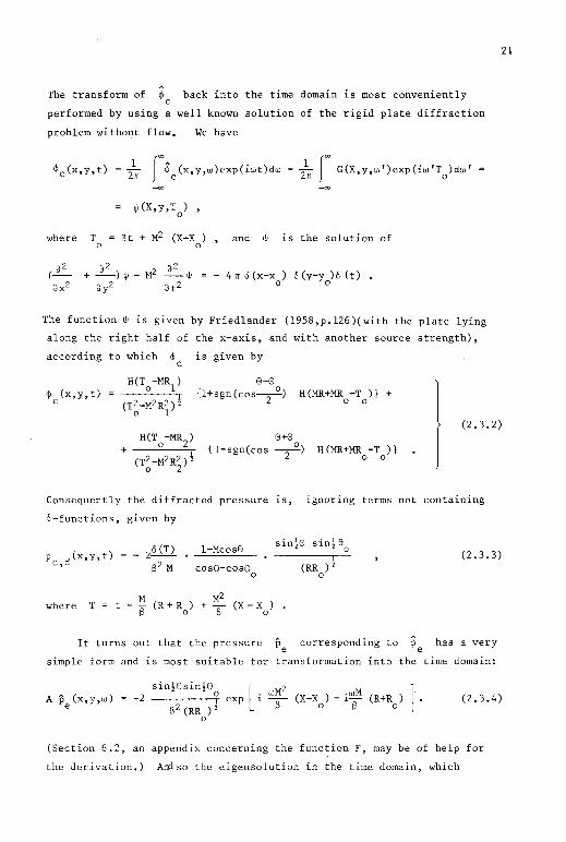
The transform of <Pc back into the time domain is most conveniently

perf ormed by using a well known solution of the rigid plate dif fraction

problem without flow, We have

<Pc(x,y,t)

where T 0

1 211

ij!(X,y,T ) 0

St + M2 (X-X ) 0

2~ f00

G(X,y,w')exp(iw'T0

)dw'

and ij! is the solution of

The function ij! is given by Friedlander (1958,p.126)(with the plate lying

along the right half of the x-axis, and with another source strength),

according to which <Pc is given by

<P (x,y, t) c

H(T0

-MR1

)

(T~-M2Ri) 2

+ H(T

0-MR

2) 1

(T2-M2R2) 2 0 2

8-8 {l+sgn(cosT) H (MR+MR -T ) } +

0 0

8+8 {1-sgn(cos --0

) 2

H(MR+MR -T )} 0 0

(2.3.2)

Consequently the diffracted pressure is, ignoring terms not containing

o-functions, given by

p d(x,y,t) c,

where T

l-Mcos8

cos8+cos8 0

(2.3.3) (RR ) 2

0

It turns out that the pressure pe corresponding to ~e has a very

simple form and is most suitable for transformation into the time domain:

A pe (x,y,w) sinj8sinj8 l wM2

-2 o exp i -0

- (X-X ) - iwM (R+R ) e2 (RR l, ,_, o e o

0

(2.3.4)

(Section 6.2, an appendix concerning the function F, may be of help for

the derivation.) An:lso the eigensolution in the time domain, which

21

22

together with the continuous solution .(2,3,3) satisfies the Kutta condition,

is

p k(x,y,t) e, A p (x,y,w) exp(iwt)dw

e

sin!e sin!e - 2 ° ,f(T)

e2 (RRo)' (2.3,5)

Note the complete agreement in time dependence of Pe,k and the pulse-

part of Pc,d • Summing these two gives

o (T) l+Mcose sinjesin!e 0

- 2 0

Pk,d Pc,d + Pe,k S2M cose+cose (RR ) '

0 0

(2.3.6)

Clearly we have

Pk,d l+M co se 0 1 when + 0 < 0 < 11 - 0 > - 11

Pc,d 1-M cos0 0 0

i.e. - 11 + e < e < 11 - e 0 0

< 1 elsewhere

l (2.3. 7)

So when we compare the smooth solution with the continuous solution at a

fixed observation point, we see from (2.3,7) that application of the Kutta

condition results in an increase of the pressure amplitude within the

symmetrie downstream wedge lel < 11 - e0

and a decrease elsewhere. Note

that this wedge angle is only dependent upon the angle e0

of the source

location, and not on the Mach number. Of course the increase and decrease

is only of Pk,d relative to pc,d' and the actual difference may be small.

Due to the sin!e term the predicted difference will be largest near the

plate, where sin!e ~ ±1 , and small near the wake, where

This is, moreover, enhanced by the convection: note that

sinje ~ o. 1 sin!e I < 1 sinl9 I

when O < lel < Î, and lsin!el > lsin!el when }- < lel < 11 As will

become clear in section 2.5, where a comparison with experiments is made,

it is not difficult to verify the upstream decrease experimentally, hut to

check the downstream increase well-chosen Mach numbers and locations of the

source are necessary.

23

2.4 The ha1'monia plane wave

Equations (2.2.1) are valid again, but now without the source term.

Instead we have a plane harmonie wave incident from below in the direction

Above the plate there is a shadow region (es,n) , Because

of convection we have e. f 6 1 s

In fact the following relation is valid

(introduce for convenience the auxiliary variable e ) : s

The basic incident wave is then

S sine s

cose - M s

q, (x,y,t) 0 .

exp [i w~2 X-i wSM (X coses + y sines) + iwt]

using the same notation as in section 2.3. Applying again the Prandtl-

Glauert transformation in the classical Sommerfeld screen diffraction

.solution (Jones (1964)) we get the following continuous solution (which

does not yet satisfy the Kutta condition)

4> (x,y,t) c,s

TI M wM2 /IT exp [ i 4 - i wS R + i -

13- X + iw t _] .

[

! 8-8 wM ! 8 +es l • F {(2 wt R)

2

sin-~}+ F {(2 T R) sin-2-}

(2.4.1)

(index s of <jl denotes "Sommerfeld"), and the corresponding pressure c,s

p (x,y,t) c,s

- iw(l-M 132

cos8 )<jl (x,y,t) --1-(2wM) s c,s s!TI s

!

• exp ( i TI4 i wM R + i wM2 ) S - 13 - X + iwt

with the aid of section 6,1.

sin je cos!es T

(2.4.2)

Since both <l>c,s and pc,s satisfy the governing equations, so must

the remaining term in (2.4.2). Moreover, this term vanishes as r +

and bas an integrable singularity in r = 0 ,

24

soit must be a multiple of the eigensolution (2.3.4). Indeed, as $ c,s

is regular as r + 0 , pc,s becomes regular ~nd so satisfies the Kutta

condition) when we cancel that term. So we have, in a very simple way,

the solution that satisfies the Kutta condition in the form

pk (x,y,t) ,s iw

(1 - M cos El ) $ (x,y,t) 62 s c,s

(2.4.3)

and, after integration of the pressure equation of (2.2.1) (use (6.1.13)),

and application of the boundary conditions at y = 0 and infinity,

$k (x,y,t) ,s

! WM2 A $ (x,y,t) -2(2M(l-M)) cos~El exp(i-;;-X +iWt}$ (x,y,w).

c,s s P o e

(2.4.4)

Solution ~c,s can be obtained from $c by taking R0

+ 00 in a proper

way, and similarly we can find the expressions for the diffracted pulse

corresponding to pc,s

reveals nothing new.

and

2.5 Comparison with experiments

from and This, however,

As far as we could trace, the most relevant experiments for the

present theory are those by Heavens (1978). He made schlieren photographs

of the density field (which is up to a factor equal to the pressure field)

around an airfoil trailing edge. Under varying flow conditions a plane

pulse was generated above the trailing edge. This pulse was reflected by

the airfoil, transmitted through the wake, and it produced a cylindrical

diffracted wave at the edge. In addition to the pulses, also harmonie

waves were applied, but Heavens drew no conclusions from the results

because of the poor quality of the pictures.

Heavens' principal results are that under the different flow

conditions only the diffracted wave changes; it is weak in smooth flows,

where the Kutta condition may be expected to apply, and it is strong in

unsteady and separated flows, where the Kutta condition is probably not

valid. (As is mentioned in section 1.3, two different external effects

may work together and suppress the viscous farces and so invalidate the

Kutta condition.) See for instance Heavens' figure 7(a) and (b).

If we take into account the fact that the pictures do not really show

an increase or decrease in the region surrounding the wake, which

would be consistent with the small sin!G factor our conclusions,

presented in and below equation (2.3.7), may very well be the explanation

25

of Heavens' findings. As far as the upstream decrease is concerned, this

is well confirmed, while the downstream increase is not refuted. Even

more, the fact that confirmation of the downstream increase would be mor

difficult is part of the conclusions. From equations (2.3.3), (2.3.5)

and (2.3.7) we can see the effect of variations of the parameters in

possible future additional experiments complementing Heavens' series of

tests. A Mach number close to (but smaller than) one enlarges the relarive

increase near the wake, but also reduces the factor sinjB fora fixed 8,

On the other hand, placing the source near the plate increases the

diffracted wave amplitude but reduces the region around the wake where the

relative increase occurs. Probably it will depend on the sensitivity of

the schlieren system how the optimal choice of the parameters is made that

reveals the behaviour of the diffracted wave near the wake.

Other experiments, worthwhile to mention, are those by Lawrencc,

Schmidt and Looschen (1951). They made schlieren photographs of ~he

density-(pressure) sound field generated by the vortexstreet behind the

blunted trailing edge of an airfoil. (Probably more experiments of this

kind have been done in the past, but these have the advantage that the

relevant pictures are reproduced by Davis (1975) and therefore readily

available.) Although these experiments do not really correspond to our

analysis, they show the appropriateness of Jones' (1972) model and his

eigensolution (2.3.4). When we, following Ddvis (1975), model the vortex

street as a vortex sheet and do not apply the Kutta condition (otherwise,

without external force, the only solution would be the trivial one), the

relevant eigensolution is Jones' eigensolution (2.3.4), of course with a

frequency and amplitude depending on the Reynolds number and StrO<Jhal

number of the real problem. The photographs show indeed the pattern,

given by (2.3.4), namely cylindrical co~vected wavefronts coming from the

trailing edge (according to (x-t)2 + y2 = (t/M) 2) with a large

26

amplitude near the airfoil and a small amplitude near the wake (according

to sinl0). Once more it is shown that it is useful to have the

eigensolution available in pressure form, rather than only as potential.

2.6 ConaZusions

The diffraction of a sound pulse and a harmonie planè wave around a

flat plate trailing edge in a moving medium has been studied. The

relevant eigensolution, already calculated by Jones (1972), is simply

obtained f rom the plane wave solution by inspection. This eigensolution

has the same source as the diffracted wave (i.e •. the trailing edge).

Therefore it will affect only, and be in phase with, .the diffracted wave.

In particular, in the pulse problem it affects only the pulse part (and

not the tail) of the diffracted pressure. Comparison of the Kutta

condition solution with the continuous solution shows an increase of the

diffracted wave in a downstream are and a decrease elsewhere. The rate

of the increase and decrease depends on the Machnumber, hut the angle of

the are does not. As far as the upstream decrease is concerned this is

very well confirmed by Heavens (1978). Although his pictures do not

contradict the downstream increase (as the wave itself is weak there) a

few additional experiments with well chosen Mach numbers and source

locations would be welcome to complement his series of tests.

chapter 3

THE INTERACTION OF A HARMONIC PLANE WAVE WITH THE

TRAILING EDGE, AND ITS SUBSEQUENT VORTEX SHEET,

OF A SEMI-INFINITE PLATE WITH A UNIFORM LOW-SUBSONIC

FLOW ON ONE SIDE

3,1 Introduction

27

Probably the simplestmodel problem with practical importance of

acoustic waves in a non-uniform medium involves an inviscid fluid with a

thin mixing layer, modelled as a vortex sheet, which séparates a uniform

flow from a stagnant flow, perturbed by acoustic waves. As far as the

acoustics are concerned, the first correct analyses of this problem were

given by Miles (1957) and Ribner (1957) for plane harmonie incident waves,

while Gottlieb (1960) extended their work for a harmonie line source. As

was demonstrated by Helmholtz in 1868 (see Batchelor (1967)) for

incompressible flow and by Landau (1944) for compressible flow, an infinite

plane vortex sheet is unstable, bath in the temporal and the spatial sense.

It seems that in every geometry involving an infinite vortex sheet there

is always one instability which can be identified with this particular

instability (actually a pair, if we include the decaying, that is growing

for negative time, complementary one). Therefore we shall refer to this

as the Helmholtz instability. Note that the expressions: instability,

instability wave, instability field, etc., will be used synonymously.

The amplitude of the Helmholtz instability wave decays exponentially with

distance from the vortex sheet, Therefore it does not contribute to the

sound field, and could be ignored by the previous authors without affecting

their main conclusions, In the initial value problem, however, as treated

for instance by Friedland & Pierce (1969) (for a line source) and Howe

(1970) ~or a point source), these instabilities must be included to obtain

a causal solution (i.e. one with no disturbances before the source is

switched on), and could not be ignored, Unfortunately, some parts of the

instability field are more singular than, say, a Dirac delta function and

28

caused some interpretational problems. Only by Jones & Morgan (1972) was

this singularity classified as an ultradistribution - loosely speaking a

distribution with complex argument - and by them the pulse problem was

solved correctly. Having then a grasp of this problem, Jones & Morgan

were able in the same paper to find the harmonie field that wo~ld arise

from a harmonie source switched on a long, finite time ago. They called

this harmonie solution "the causa! solution". In it the Helmholtz

instability wave is present with a uniquely defined amplitude, and this

solved the riddle of the undetermined instability amplitude for this

harmonie problem; not for the genera! one. For example, the problem that

should model a real physical_harmonic source/mixing layer interaction is

not yet solved by Jones & Morgan's causa! solution, because in reality the

memory of the system cannot be very long with the inherent variety of

additional perturbations. But still the experiments (Poldervaart et al

(1974)) show a perfect reproducibility, so another mechanism must be

responsible for the choice of the eigensolution (i.e. Helmholtz instability)

amplitude.

As we will show in the following sections, the mathematically

sufficient condition, which is also physically much more acceptable than

causality, is the choice of the level of singularity at the trailing edge:

"the Kutta condition", or otherwise. In the problem discussed so far no

solid boundary with a trailing edge was included, but this is obviously

only a simplification of the reality. Of course the edge may be far

enough away in some problems for us to neglect it, as in some initialvalue

problems, but in the harmonie problem all of the vertex sheet is perturbed

and the influence of the edge is not, a priori, small. In fact, in our

linear model it becomes larger as the edge is taken further away.

Our conclusion is that the doubly-infinite vertex sheet model with

harmonie perturbations is too much simplified, resulting in a basically

undeterminable Helmholtz instability amplitude. Therefore, we shall

consider in this chapter only the model of a semi-infinite vortex sheet

downstream a flat plate with harmonie disturbances. Extending the ideas

of Jones & Morgan (1972) the semi-infinite vortex sheet problem was solved

by Crighton & Léppington (1974) and Morgan (1974). Although their

solutions are correct, in our opinion, they insisted in the derivation of

the harmonie solution on the application of the causality criterion and

on}y in the last resort on the Kutta condition. They did not realise that

the Kutta condition was sufficient to ensure uniqueness, although Crighton

& Leppington found that the Kutta condition virtually implied causality,

To clarify this controversial subject in particular, we shall devote the

next section (3,2) to it, In section 3,3 we shall formulate the problem

considered in this chapter. It is a variant of Crighton & Leppington's

and Morgan's problem. Instead of a pointsource we have plane waves, with

fronts perpendicular to the plate, coming from upstream infinity in the

subsonic flow. A formal solution will be derived in section 3.4.

Although this solution is essentially already given by Crighton &

Leppington and Morgan, we shall still repeat the calculations to show

explicitly how the causality criterion can be neglected. Finally, in the

29

last sections we shall calculate the near and far field in the low Mach

number limit. This has not been dorre before, although it was proposed by

Crighton & Leppington (1974). In the case treated here, the incident wave

is simple enough to enable an explicit approximation to be derived. Use

is made of an elegant technique, proposed by Boersma (1978), to evaluate

a complex integral approximately. It is explained in section 3.5

separately, to ease the use of it again in chapter 4. As far as the

acoustics are concerned the approximation is uniform from the near field

to the far field, except for the bow wave which together with the

instability wave is only calculated in the near field. Their f ar field

would require much additional calculation, of which the worth is dubious

since the vortex sheet does not model a mixing layer very well in that

region.

We finally have to note that the case of a supersonic flow seems to be

very different, An attempt to include this is not given here. Morgan

(1974) found that in the relevant eigensolution the vortex sheet is

discontinuous at the edge, and that the vortex sheet in the least singular,

vortex shedding, solution still leaves the edge with a finite slope (and

so with discontinuous derivative). This is not observed in experiments.

As with the l//r edge singularity of the subsonic eigensolution, the

discontinuity will probably be due to the improper linearisation. An

explanation for the finite slope may be that we do not recognise Morgan's

findings either because the slope is very small, or because it is not yet

achieved experimentally. The vortices we see in the existing experiments

are shed (according to this conjecture) in the subsonic region of the

boundary layer and deceive our observations of a satisfied Kutta condition.

30

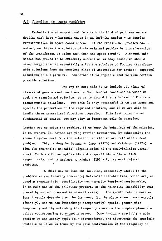
3.2 CausaZity vs Kutta aondition

Probably the strongest tool to attack the kind of problems we are

dealing with here - harmonie waves in an infinite medium - is Fourier

transformation in space coordinates. If the transformed problem can be

solved, we obtain the solution of the original problem by transformation

of the transformed solution back into the space domain. Although this

method has proved to be extremely successful in many cases, we should

never forget that it essentially sifts the subclass of Fourier transform­

able solutions from the complete class of acceptable (or rather: expected)

solutions of our problem.

possible solutions.

Therefore it is arguable that we miss certain

One way to cure this is to include all kinds of

classes of generalised functions in the class of functions in which we

seek the transformed solution, so as to extend that subclass of Fourier­

transformable solutions. But this is only successful if we can guess and

specify the properties of the required solution, and if we are able to

handle these generalised functions properly. This last point is not

fundamental of course, but may play an important r8le in practice.

Another way to solve the problem, if we know the behaviour of the solution,

is to prepare it, before applying Fourier transforms, by subtracting the

known singular part from the solution, so that we are left with a neat

problem. This is done by Orszag & Crow· (1970) and Crighton (1972a) to

find the (Helmholtz unstable) eigensolution of the semi-infinite vortex

sheet problem with incompressible and compressible subsonic flow

respectively, and by Bechert & Michel (1975) for several related

problems.

A third way to find the solution, especially useful in the

problems we are treating concerning Helmholtz instabilities, which are, as

growing exponentials, specifically not normally Fourier-transformable,

is to make use of the following property of the Helmholtz instability· (not

proved by us but observed in several cases). The growth rate is more or

less linearly dependent on the frequency (in the plane sheet case: exactly

linearly), and we can interchange (temporarily) spatial growth with

temporal growth by extending the frequency space to the complex plane via

values corresponding to outgoing waves. Once having a spatially stable

problem we can safely apply Fo,·~;ertransforms, and afterwards the spatially

unstable solution is found by analytic continuation in the frequency of

31

the stable solution to real frequencies.

When we apply the causality criterion, we come across this lastmethod

rather naturally. This does not imply, however, that our solution should

be causal. The method is only one of the devices to obtain the solution,

and combined with the Kutta, or an analogous, condition, they all realise

the ~ unique solution. Moreover, it would lead to contradictions, if

we were to insist on causality, irrespective of the prescribed level of

singularity at the edge. Causality requires regularity of the solution

in some halfplane of the complex frequency space (Jones & Morgan (1974)).

In a viscous flow the level of singularity at the trailing edge is governed

by viscous farces and a function of frequency and amplitude (among others).

Examples are given in chapter 5. The corresponding amplitude of the

singular eigensolution is therefore dependent on the frequency, but

obviously not necessarily in an analytic way. It would be very artif icial

to expect the viscous farces to take into account the start of the acoustic

source very long ago.

Finally, we note the following argument to explain why the Kutta, or

an analogous, condition virtually implies causality. According to a

theorem, found by Bechert & Michel (1975) for incompressible flow and by

Howe (1976) for compressible flow, the semi-infinite vortex sheet problem

has only one eigensolution, namely a Helmholtz instability which does not

satisfy the Kutta condition. It can be interpreted as the result of

vorticity shed from the edge. In the cases considered, vorticity can only

be shed by external means. When a sound wave passes the edge without

shedding vertices (the Kutta condition is then as a consequence not

satisfied), we get the stable solution without exponential growth of the

vortex sheet displacement amplitude. The more vorticity is shed the more

of the eigensolution must be included, until finally the Kutta condition is

satisfied. Therefore the whole field is determined by the source via the

shed vorticity, and is thus causal, in the sense that the source causes the

disturbances. When in particular the Kutta condition is applied the above-

mentioned theorem precludes perturbations (eigensolutions) without a

source and now the solution is also causal in the strict sense of Jones &

Morgan (Morgan (1974)). When we prescribe a level of singularity other

than that with the Kutta condition, vorticity is also shed without a source

and the field is not zero before the source is switched on, and therefore

this field is not causal in the sense of Jones & Morgan. This, however,

32

is not in contradiction with the reality because the complete problem is

non-linear and the amount of shed vorticity is dependent upon the

amplitude of the source: zero amplitude means zero vorticity, therefore

zero field and thus we still have causality.

~ Fo!'mUZation of the probZem

In the (x,y) -space a compressible inviscid fluid flows subsonically

in the lower half space (y < 0) in the positive x direction with the

dimensionless velocity (1,0) •. In the upper halfspace (y > 0) the fluid

is stagnant, while the two halfspaces are separated by a flat, rigid plate

in y = 0 ' x < 0 and a vertex sheet in y = 0

' x > 0 Everywhere

the dimensionless density is 1 the sound speed M-1 The fluid is

perturbed by plane harmonie waves, coming from upstream in the flow with

wavefronts perpendicular to the plate. A sketch is give.n in figure 2.

stagnant fluid

plate

incident plane waves

c::=> main flow

y-axis

diffracted, and instability/edge-interaction wave ,.,...-

- ·:::.:::: = = -=---: - / unsta bie '~ ~, vortex sheet '~,

.... ~~

primary wave

Figure 2

The dimensionless perturbation quantities are (u,v) for the velocities

and p for the pressure. Later we shall introduce the auxiliary function

v of variable u , but we shall never use the velocities (u,v)

explicitly so this will cause no confusion. The perturbation amplitudes

are considered to be small enough to justify the sound speed being taken

33

as constant and the perturbation of the vortex sheet position being

negligible. The regions containing vorticity are consequently restricted

to lines (surfaces in the complete 3-dimensional space) and we can

introduce a potential ~ ' defined by v~ = (u,v). The Kutta condition

may be satisfied or not. For convenience we write explicitly

~ = ~o + ~ = ~o + ~c + B ~e , where ~o is the incident wave, ~e is

Crighton's U972a) eigensolution (Helmholtz unstable, not satisfying the

Kutta condition, representing shed vorticity), ~o + ~c is the stable

solution (in which no norticity is shed), and ~o + ~c + Bk ~e = ~o + ~k

is for a particular choice B = Bk the solution that satisfies the Kutta

condition. The index k stands for Kutta and the index c recalls the

analogy with the continuous solution of chapter 2. The Strouhalnumber, or

dimensionless frequency, is w the Machnumber, or reciprocal of the

dimensionless sound speed, is M and the Helmholtznumber, or dimension-

less wavenumber, is k = wM In this problem the only lengthscales are

the acoustic wavelength (the quotient of sound velocity and frequency) and

the hydrodynamic wavelength (the quotient of flow velocity and frequency).

Therefore we can take either w = 1 or k = 1 • Yet we leave them

unspecified, because the results of this chapter will be used later in

chapter S, where viscous effects are included, and a third lengthscale

appears which will then be used as the most convenient reference length.

We suppose that the variables do not depend on the dimensionless time

coordinate t in any way other than through the factor exp(iwt), which

will be suppressed throughout.

Linearising, we have the following equations and boundary conditions

(the index x denotes differentiation to x , similarly for y ) :

~o(x,y) 0 in y > 0

exp(- k l+M x) in y < 0

M + k2 ~ 0

) in y > 0 ' (3.3.1)

p - i w ~

34

+

p

k2 lji - 2 i k M lji X - M2 lji XX

- i w $ - iw lji l+M o

0

} in y < 0 '

lji (x,O) y

0 in x < 0 , since the plate is rigid,

"' + 0 when jyj + 00 , since the field radiates outwards,

iwlji(x, +O) - iwlji(x,-0) - ljix(x,-0) in x > 0 ,

(3.3.2)

(3.3.3)

(3.3.4)

(3.3.5)

since there is no pressure difference across the vortex sheet, When

y = h(x) exp(iwt) represents the position of the vortex sheet, we have

i w h(x) lji (x,+O) y

i w h (x) + h (x) x

lji (x,-0) y

} in x > 0 ,

since the vortex sheet is a material surface. The vortex sheet is

(3.3.6)

1

continuously connected to the edge, which will imply that h(x) = O(x 2)

(x f 0) , and when the Kutta condition is applied we will have

h(x) = O(x3/ 2) (x f O) , The net force on the plate is fini te so the

pressure difference across the plate is (at least) integrable, For

convenience we give k an imaginary part (or rather w , as we keep M

real), k = jkj exp(-io) where 0 < 8 < 11 the field being outward

radiating.

3,4 FoPmaZ soZution

To keep comparison simple we shall adopt the nomenclature of Jones &

Morgan, with the extensions introduced by Munt (1977) in his studies on the

circular jet. Introduce the Fourier transf orm of iµ

$ (s ,y) r"' (x,y) exp(-sx) dx ' s complex, (3.4.1)

Define in the complex s-plane the following halfplanes

35

hl . Re s > - sine l+M

Re s < Jkl sine

called the (t) plane

} (3.4.2)

called the e plane

Indices + and will denote regularity in the (t) and e plane

respectively. The strip - (l+M)-l !ki sine < Re s < lkl sine

connnon to the (t) and the e planes ' will be called the strip of overlap.

Following the same lines as Munt (1977) or Morgan (1974), we introduce the

Fourier transform of h

r h(x) exp(- s x) dx

0

(3 .4. 3)

and the Fourier transf orm of the pressure dif f erence across the plate

(multiplied by M), as far as it is induced by field ~

G_(s) r [ik~ (x,+O) - ik~ (x, -0) - M~ x (x,-0)] exp (-sx)dx

We introduce the complex functions

Branchcuts run from ik

-ik(l + M)-l to -ik 00

defined by

+ \;(o)

! Àl (0) 1 k I'

À~(O) \;(o) 1

lkl 2

and -1

ik(l-M)

respectively.

+ ! where Àl (s)=((l+M)s+ik)',

- ! Àl (s)=((l-M)s-ik) 2

,

+ where \2

(s) !

(s+ik) 2

! (s-ik) 2

to ik 00 , and from -ik

The appropriate branches are

exp ( i Î - i l e) ' and

exp (-i ~ - i l e) 4

(3.4.4)

(3.4.5)

and

Transform the equations (3.3.1) and (3.3.2), and solve the resulting

equations for s in the strip of overlap, applying (3.3.4) and using the

36

are negative in the strip. Transform the fact that Im Àl and Im À2

boundary conditions (3.3.3),

integration constants of the

(3.3.5) and (3.3.6), and determine the

recently found transformed solution, to get

l k F+(s)

(- i À2

(s)y) when y > 0 M À2(s) exp

~(s,y)

ik+Ms F+(s) (i Àl (s)y) when y < 0 ---rM • Àl (s) exp

} (3.4.6)

together with the functional equation

G_(s)

where

+~ 1 l+M • --:-n

s l+M

X (s) 1 k \ (s)

k3 - i _M_\_(_s..;.;)-À2_(_s_) x(s) F+(s) (3.4.7)

(3.4.8)

is the crucial function of the analysis. X(s) = 0 is the dispersion

relation for the possible waves in the vortex sheet. X has (for M < 1)

' two zeros: s0

and s1 , corresponding to the' increasing and decreasing

Helmholtz instability waves. For convenience we write explicitly

X(s) 1 (s - s 0

) (s - s1

) µ (s) (3.4.9) k2

and

s - ik u - ik! (ç; +in) 0 0

) sl - ik u1 - ik ! (ç; - in) (3.4.10)

1

where ç; = (1 + (1+M2 )2) M-1 ' n = (2/;;M-l-l)j

The derivation of the expr~ssions for

Morgan (1972).

s and 0

can be found in Jones &

We will now solve equation (3.4.7) by means of the Wiener-Hopf

technique. A good introduct_ l with detailed examples is given by Noble

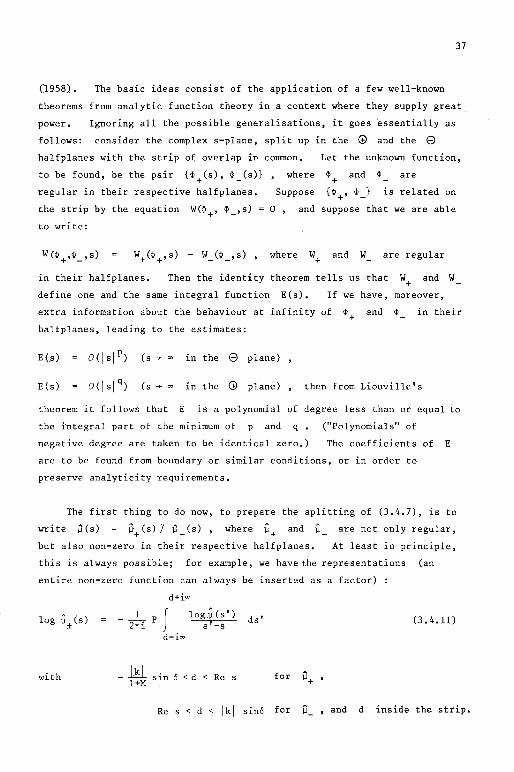
37

(1958). The basic ideas consist of the application of a few well-known

theorems from analytic function theory in a context where they supply great

power, Ignoring all the possible generalisations, it goes essentially as

follows: consider the complex s-plane, split up in the <±> and the e halfplanes with the strip of overlap in common, Let the unknown function,

to be found, be the pair {4+(s), 4_(s)} where 4+ and ~ are

regular in their respective halfplanes, Suppose {$+' 4_} is related on

the strip by the equation W(4+' ~ ,s)

to write:

0 , and suppose that we are able

are regular

in their halfplanes, Then the identity theorem tells US that W+ and W

define one and the same integral function E(s), If we have, moreover,

extra information about the behaviour at infinity of 4+ and 4

halfplanes, leading to the estimates:

in their

E(s) in the 8 plane)

E(s) o<I si q) <s _,_ 00 in the <±> plane) then from Liouville's

theorem it follows that E is a polynomial of degree less than or equal to

the integral part of the minimum of p and q

negative degree are taken to be identical zero,)

("Polynomials" of

The coef f icients of E

are to be found from boundary or similar conditions, or in order to

preserve analyticity requirements.

The first thing to do now, to prepare the splitting of (3.4.7), is to

write ;J(s) D+(s) / (l_(s) , where µ+ and il are not only regular,

but also non-zero in their respective halfplanes. At least in principle,

this is always possible; for example, we have the representations (an

entire non-zero function can always be inserted as a factor) :

with

--P 27ri

d+ioo

f log\;(s')

s'-s d-ioo

hl sin o < d < Re s l+M

ds' (3,4.11)

Re s < d < lkl sinê for Q_ , and d inside the strip.

38

The capital P means that the principal value may be taken if necessary

(Noble (1958), p. 42 ; see also (3.5.1) ).

When the complex value of k is close to real values (i.e. o small), we

have s 0

E 8 plane and s 1

E ® plane furthermore

- ik (l+M)-l E @ plane, so it follows readily that a splitting of

equation (3.4.7) is then achieved by

G_(s) À~(s) 9s>µ _ (.s) +

s - s 0

(s) À~(s) 9s> A -ik - -ik - -ik

ik 1 [µ _ µ - (l+M ) Àl(l+M) À2(1 +M)j l+M ~

+ ik s-r-!- - s-s

0 -- + s l+M l+M 0

ik(s-s1) IJ+(s) F+(s) A -ik - -ik - -ik

ik µ_ (l+M) À{li:M) À2(l+M) 1 +-- ik ik l+M + À+ (s) À+ (s) l+M s s + l+M M 1 2

0

E (s) ,

where E is an entire function. It is easiest to bring

left because F+(s) must be regular in the (f) plane •

leave s - s 0

in the right hand side of (3.4.12), E (s)

(3.4.12)

s - s to the 0

If we were to

would have to be

chosen in a way to eliminate the pole s = s0

from F+ and the result

would be the same. Standard methods provide the estimates

p+ Cs} = o<lsl !> (s _,. 00 in the G:l plane), il (s) =oei si-!> (s _,. 00 in

the 8 plane) and (from h(x) = O(x!}(:X + o)) F (s) = O(lsl-3/ 2) + 1

(s-+ 00 in the ® plane). It follows that E(s) = O(lsl-) (s-+ 00 ) ,

theref ore E _ 0 • Now it is possible, by reordering the terms of

(3.4.12), to obtain G and F+ explicitly. We see that

G_(s) = O(I si-!) , so indeed the pressure difference across the plate is

integrable. Only F+ is important for the solution ~ , via (3.4.6).

As was anticipated before, in section 3.2, we found here by straight­

forward application of Fourier transformation only the Fourier transform­

able solution, that is the stable solution ~c , where no vorticity is

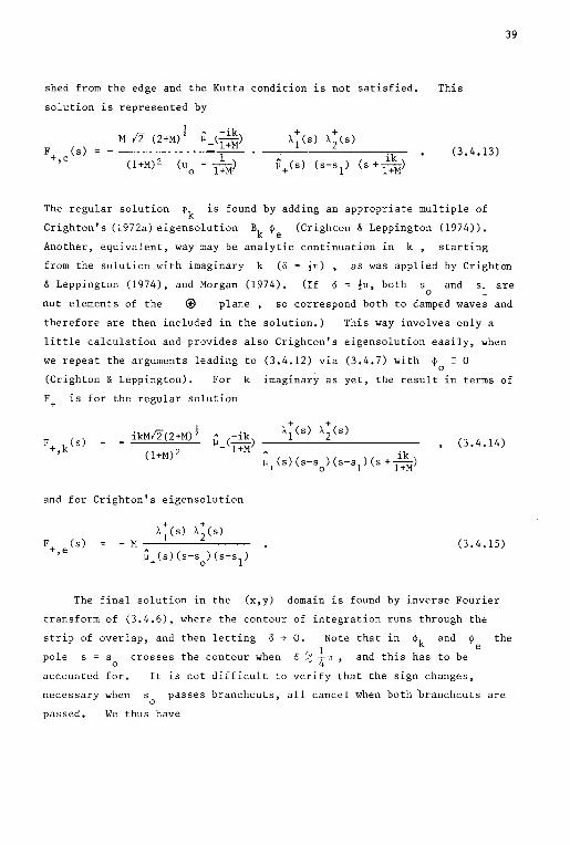
shed from the edge and the Kutta condition is not satisfied. This

solution is represented by

F (s) +,c

1

M /2. (2+M) 2

(l+M)2 (u 0

µA -ik

(l+M) (3.4.13)

39

The regular solution ~k is found by adding an appropriate multiple of

Crighton's (1972a) eigensolution Bk ~e (Crighton & Leppington (1974)).

Another, equivalent, way may be analytic continuation in k , starting

from the solution with imaginary k (o = jn) , as was applied by Crighton

& Leppington (1974), and Morgan (1974). (If jn, both s and 0

not elements of the plane , so correspond both to damped waves and

therefore are then included in the solution.) This way involves only a

little calculation and provides also Crighton's eigensolution easily, when

we repeat the arguments leading to (3.4.12) via (3.4.7) with ~o - 0

(Crighton & Leppington). For k imaginary as yet, the result in terms of

F+ is for the regular solution

;; eik) l+M (3.4.14)

ikM/2 (2+M) j

(l+M)2 ik µ + (s) (s-s

0) (s-s 1 ) (s + 1 +M)

and for Crighton's eigensolution

F (s) +,e

+ + Àl (s) À

2(s)

- M ~~~~~~~~-); (s)(s-s )(s-s

1)

+ 0

(3.4.15)

The final solution in the (x,y) domain is found by inverse Fourier

transform of (3.4.6), where the contour of integration runs through the

strip of overlap, and then letting o +

pole s = s0

crosses the contour when

accounted for. It is not difficult to

o. No te that in ~k and ~ 1

0 ~ 4n' and this has to be

verify that the sign changes,

the e

necessary when s0

passes branchcuts, all cancel when both branchcuts are

passed. We thus have

40

l/J(x,y) lirn ~ li+O 211:1.

i 00-o

= 2!i f -ico+o

ioo

f $(s,y) exp (sx)ds

-io:i

~(s,y) exp (sx)ds + ,- [<s-s )~(s,y)exp(sx)] -] o s=s - 0

(3.4.16)

k,e

The strip of overlap is collapsed into the irnaginary axis and now the

contour of integration runs along the irnaginary axis: at the right side of

the branchcuts and pole when Irn s < - k(l+M)-l , and at the left side of

the branchcuts when Irn s > k

At this stage of the analysis it becornes convenient to introduce the

followingtransforrnation and substitutions:

s - iku,

µ(s) = µ(u),

µ+(u)

kw(u) 1

k((l-uM) 2 - u2) 2 ,

lkexp(i!11) (1-(l+M)u}!

Ä~(s) = Ik exp(-ij11) w_(u) = lkexp(-il11) (1+(1-M)u) ! ,

~ Ä2

(s) = k v(u) = k(l-u2)- ,

+ Ä

2(s) Ik exp(ij11)v+(u)

l = lkexp(ij11)(1-u) 2

Ä;(s) Ik exp(-i!11)v_(u) !

= lkexp(-i!11)(l+u) 2

the ® plane in the u-plane is Irn u ~ 0 . the e plane in the u-plane is Irn u :; 0

(3.4.17)

The square roots v+ and w+ are, chosen this way, principal branches.

Note that x(-iku) = A(u) in the terrninology of Jones & Morgan.

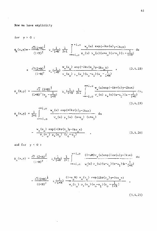
Now we have explicitly

for y > 0 :

1

\(x,y):c- /2(2+M)2

(1 +M)2

+

(l+M)2(u __ l_) o l+M

co+i.o

~e (x,y) = _l_ f 't' 21Ti

- 00-i.o

w+(u) exp(-ikv(u)y-ikux)

v_(u) µ+(u) (u-u0

) (u-u1

)

w+(u ) exp(-ikv(u )y-iku x) - 0 0 0

v (u ) µ (u ) (u - u ) - 0 + 0 0 1

and for y < 0

41

(3.4.18)

(3.4.19)

du

(3.4.20)

! /2 (2+M) 2

00+i.o

µ_(l~M) 2;i f (1-uM)v+(u)exp(ikw(u)y-ikux)

du

(l+M) 2

fi(2+M)l

(l+M) 2

- 00-i.o

1 (1-u M) v (u ) exp(ikw(u )y-iku x) () o +o o o

µ_ l+M w (u) µ (u )(u -u )(u --1-)

- o + o o 1 o l+M

(3.4.21)

42

/2 (2+M)! (1-uM)V+(u)exp(ikw(u)y-ikux) 1 du ,

w_ (u) µ + (u) (u-u1) (u - l+M) -oo-i.o

(3.4.22)

Joo+i.o(l-uM)v+(u)exp(ikw(u)y-ikux)

w_(u) µ+(u)(u-u0

)(u-u1

) du

-oo-i.o

(l-u0

M) v+(u0

) exp(ikw(u0)y-iku

0x)

+ ~~=-~~~=-~~~~~=-~~~-=-~ (3.4.23) w_(u

0) µ+(u

0)(u

0-u1)

The multiplicative factor Bk is given by

(3.4.24)

The integration contours run along the real axis in the u-plane, on the

negative interval just below the branchcuts, and on the positive interval

just above.

In the problem considered the~sound waves propagate in the same

direction as the flow, and inside the flow, Therefore the problem may be

not general enough to justify the general conclusions drawn above with

respect to causality and the Kutta condition. However, extensions to

include oblique wavefronts, coming from the side of the flow or the

stagnant region, are easily made, They show that for all angles of

incidence of a wave coming from the still region (essentially the Crighton

& Leppington (1974), and Morgan (1974) problem) the above calculations are

the same, besides some trivial alterations. An:lin the case of a wave

coming from the flow the calculations are the same as long as the point of

reflection on the vortex sheet moves supersonically for an observer in the

stagnant region, That means that the angle of incidence is not too close

to the negative flow directiqn (see equation (3.4.25) below). Otherwise

43

we would have so-called "total reflection" (Mi les (195 7), Ribner (195 7)),

in which case we have to modify the mathematics substantially. Although

we have not proved it, the general conclusions then still seem to apply.

We illustrate the previous arguments with some details. Consider an

incident wave, coming from the flow, of the kind used in the airfoil

diffraction problem (section 2.4)

where

given by

exp(-ik

S sin G s

cos G -M s

cosG -M ___ s_x)

and the angle of incidence

Then equation (3.4.7) becomes

G (s) + ik 1-Mcose

s case - M

s + ik---s __

e. 1

0<8i<TI, is

(3.4 .25)

cos G - M in the strip of overlap sinó s

< Re s < 1k1 sin 6

l 1 Total reflection occurs when - M2 (2+M) 2 < tg 8. < 0 , in which case the

1

strip is empty. Apparently it is not enough merely to subtract off the

primary wave. The difficulty is presumably cured by removing the waves

reflected and transmitted by the vortex sheet, as well as the primary wavP..

This difficulty does not seem to be related to the one encountered by Jones

& Morgan (1972,p.485). They found that when the source receded to infinity

via a ray within a certain wedge, no limit to the solution was found, and

in particular, the plane wave case was not recovered. We, however, did

find a solution for plane waves coming from these angles, and conclude that

the angular and radial limits involved are not interchangeable.

44

~ Approximation of the split [unations

A main object we pursue in both this chapter and the next one (4), is

an explicit expression for the formal solutions, which are, though cat1plet~

not easily interpretable. Obviously this can only be achieved asymptotic­

ally. One of the parameters of the problem will be confined to the

neighbourhood of one of those critical points which allow in the limit an

asymptotic expansion of the formal solution in elementary functions.

Several choices are possible. The choice in this chapter (3) will be of

Machnumber close to zero (0 < M << 1), and in the next chapter (4), of

Strouhalnumber close to zero (0 < w << 1). In both,problems the central

snag is the approximate splitting of the function µ(u) = µ+(u)/µ_(u) •

In both cases we shall tackle this problem in essentially the same way.

Therefore we shall explain the basic idea in general in this section, to

have it ready for application later.

It was already noted in equation (3.4.11) that a possible expression

for µ± (unique modulo an integral non-zero function as a factor) is

given by

oo+i.o

log µ±(u) 1

J log µ (u') du' 21Ti p

-oo-i.o u'-u

N+i.o 1 lim J

log µ (u') du' (3.5.1) 21Ti N->oo u'-u

-N-i.o

where u is element of the respective halfplane. It is important to

observe that the contour of integration is not necessarily fixed. From

Cauchy's theorem for integrals of analytic functions, it follows that we

may deform every finite part of the contour, provided we remain inside the

region of analyticity of logµ(u) , and incorporate the contribution from

the pole u' = u whenever crossed. Now if we can approximate µ(u)

in some part D of the complex plane by (say) µ(u) with a relative

accuracy of O(E) (E small) , i.e. µ(u) = µ(u)(l + O(E)) and D is

large enough and sufficiently well-shaped to enable us to deform the

contour of (3.5.1) into one which is completely inside D then we can

construct approximations for µ1

,

that their relative accuracy is also

valid everywhere, and we can show

O(E) Note that it is aften not

necessary to have the approximations valid everywhere, because we only

need them on the integration contour of the complete solution ~ , and,

moreover, we can perhaps apply for ~ the same contour deformation into

region D as used for µ1

45

For definiteness we assume that µ(u) = µ(u)(l+O(E)) uniformly in u

in the whole complex plane, except near one point, the real number u = a ,

lying on the positive branchcuts. When ju-al ~ O(b) , where b << a

(otherwise the region near the origin, between the positive and negative

branchpoints, is included and this makes things needlessly complicated),

we assume 1 µ (u) - iJ (u) 1 /µ (u) to be not smal 1 (enough). Obviously we

take iJ(u) to be analytic and non-zero in all the relevant regions (see

figure 3).

~I U€[

'~" indented part

)ij _ç;

"' E

real axis contour of int rat1on

\ a / branch cuts ' /

reglörl' of non uniformity

Figur>e 3

To start with, we consider u outside the a + O(b) region, hut

inside the €J plane • Deformation of the integration contour into the

one sketched in figure 3 (everywhere the old contour, except for a semi-

circle in the (:!;> plane around a wi th a radius much larger than b ) ,

does not really change equation (3.5.1) :

46

1 211i p

(+i.o -co-i.o

log µ(u')

u'-u du' where the c in the

integral sign denotes the deformation. However, naw we can apply the

approximation log µ = log µ + O(E) , and get, when we bring the contour

back into its original position with the assumed analyticity of µ(u) ,

log µ+(u) 1 211i p

-oo-i•o

1 211i p

-oo-i.o

log iJ (u')

u'-u

log iJ (u')

u'-u

du' + O(E)

du' + O(E)

Therefore, when we write µ also in split form: iJ

µ+(u)(l + O(E)) (uniformly in u in the (tl plane and outside

the a + O(b) region). (3.5.2)

In the case when u is an element of the a + O(b) region, we have to

account for the contribution from the pole u' = u • This pole iscrossed

bath in the deformation of the contour into the position of figure 3:

oo+i.o

log µ+(u) 2!i p f -oo-i.o

log Î.Ï(u') du' + log µ(u) + O(E) , u' - u

and in its deformation back into the original position:

log µ+(u) 1 211i p

and theref ore

oo+i.o

f -oo-i.o

log jJ(u')

u' -u du' + log µ(u) + O(E) ,

il (u)

il (u) µ (u) (1 + O(E)) + i!(u)

(uniformly in u in the (tl plane).

(3.5.3)

47

Note that outside the a + O(b) region (but inside the © plane)

equation (3.5.3) is also valid, being equivalent to (3.5.2), because

- µ ( 0( )) - îJ(l+O(E)) (1 0( )) î1 (1 + O(E)) • \1 +:- 1 + E = \1 + ·- + E = +

µ µ

Furthermore, the restrictions we made with respect to u being an element

of the €) plane are superfluous in the result, as we will see, and only

necessary in the proef and derivation, where usewas made of (3.5.1).

Following the same arguments as in the above, we find for µ_(u) ,

with u in the e plane : µ_(u) = îi (u)(l + O(E)) uniformly for u

in the 8 plane. Via µ+(u) = µ(u)µ_(u) = µ(u)µ_(u)(l + O(E))

µ+(u)µ(u)/îi(u)(l + O(E)) we see that (3.5.3) is realy valid everywhere.

In an analogous way the above results can be found toa for µ , and for a

real number a' (instead of a) lying on the negative branchcuts.

up everything, we have

Summing

for a on the positive real axis

µ+(u) µ+(u)µ(u)/µ(u)(l + 0( E))

(uniformly in u ) µ_(u) µ - (u) (1 + O(E))

(3.5.4)

and for a' on the negative real axis

µ+ (u) îi+(u)(l + O(E))

(uniformly in u ) (3.5.5) µ (u) µ (u)îi (u) /µ (u) (1 + O(E))

When more points a and a' are involved, the extensions are analogous

and obvious, and will not be given here. Equations (3.5.4) and (3.5.5)

may be useful, but in the cases we consider, p is still toa complicated

to permit (3.5.4,5) to be generally applicable. We shall use the simpler

form (3.5.2) in the more general evaluations of ~ (with the contours

indented as in figure 3), and (3.5.4,5) when only a fe~ pole contributions

are relevant.

48

3. 6 Approximation [or small Maah nwnber

Outside the regions u = ± 1 + O(M) it is straightforward to

approximate

w(u) v(u) (1 + O(M))

µ (u) M2 v(u) (1 + O(M))

and, applying section 3.5

v+(u) (1 + O(M))

µ (u) (M2 v_(u)rl (1 + O(M)).

From the exact expressions (3.4.10) it is easily deduced that

u 0

l+i M (1 + 0(M2)) ,

1-i (1 + O(M2)) • M

)

(3.6.1)

(3.6.2)

(3.6.3)

(3.6.4)

(3.6.5)

Note that these only suf f ice in the factors -:-1 (u - u0

, 1) of the

integrands if

hood of u = 1

/ u - u 1 / » M • As u = (1 + M) -l is in the neighbour-o,

which lies on the positive branchcuts, we may apply

(3.5.4); therefore use (3.6.4), and we have

[M2 v_( 1!M>r1 (l+O(M)) = ~ /2 M-2 (l+O(M)) (3.6.6)

The factors of the integrals (3.4.18,21) and (3.4.19,22), i.e. $k and

$c , are then

/2. (1 + 0 (M) ) M2

~ exp (-i}c )(l • O(M)). )

(3.6.7)

As was anticipated before in section 3.5, we deform the contour of

integration for the integral expressions of ~k , ~c and ~e from its

position along the real axis into one on which the ± 1 + O(M) and the

(1 ! i)M-l + O(M) regions are avoided (the regions of non-uniformity).

Another desire, however, on technical grounds, is the deformation of

the contour into the so-called contour of stationary phase.

(outside the flow) this contour is given by the hyperbola

u cos(8+iT) ( T real, - oo < T < oo) ,

and for y < 0 (in the flow) it is given by

u - .!!._ + l cos (G+i T) , sz sz

where we have used some nomenclature of chapter 2, namely 1

x = r case = SX = SR cosG , S = (1 - M2 ) 2 (see figure 4)

)

For y > 0

(3.6.8)

On these

stationary phase contours the arguments of the exponentials of the

integrands are imaginary: -ikux - ikv(u)y ikr cash T ,

- ikux + ikw(u)y = iKMX - iKRcoshT (k SK). Of course, when the

49

poles u = u0

, u1

or branchcuts are crossed, we have to account for that.

We shall try to combine the two ambitions - avoiding the trouble regions

and having a stationary phase contour - as far as possible.

When e is not in an O(/M)-neighboerhood of 0 , TI or - 7T, and

not in an O(M2 )-neighbourhood of l n or - ln the stationary phase

contours are completely outside the regions of non-uniformity, and we can

employ the approximations (3.6.1,3,5,7) for arbitrary kr When 8 is

arbitrary, we have to indent the stationary phase contour in an appropri­

ate manner to stay outside the regions of non-uniformity (see figure 4),

50

before we may apply the approximations (3,6,1,3,5,7), But then we may

deform the contour again to have it still in the stationary phase position,

So these restrictions on e are not necessary. There is, however,

another difficulty which naw does introduce a restriction on e For

convenience, we did not use the exact expressions for u 0

and ul hut

rather the approximated ones. This is qui te in agreement with the

accuracy considered, except for the instability wave. In the downstream

wedge n < e < 2':. - 4 4 (approximately), where the instability wave becomes

large, the error O(krM) of its argument yields for kr >> 1 an

exponentially large error in the wave amplitude itself. Hence we must

have in TI TI - 4 < e < 4 the restriction kr ~ 0(1). This is nothing to

worryabout, as far downstream the linear model of a vortex sheet is not

correct in any case. Concluding the above, the approximations of

~k' ~c and ~e we will construct along the lines just sketched, are valid

for kr arbitrary, when lel> !n + O(M2), and kr~O(l) otherwise. (3.6.9)

Note that these restrictions are mainly due to the instability wave, and can

be relaxed as far as the acoustics are concerned. When we ignore the

instability wave , we have kr arbitrary, except when 0 < e ~ O(IM).

Here kr ' 0(1) is necessary, because otherwise the bow wave becomes

important, as amore detailed analysis shows. If required, of course, the

instability wave can be included everywhere by using the exact expression

of u0

(3.4.10) in the argument of the relevant exponential function.

real axis 1

-1-M --------------~,--

Figure 4

e Uo

indented contour of stationary p'iase

After the application of the deformations and approximations, and

introduction of the notations

x

y

k

u 0

r cos8 ex

r sin8

8K ,

cos(e +ii: ) 0 0

8Rcos8

RsinG ,

- M 8-2 + 8-2 cos(G +i'i' ) 0 0

where eo > 0 ' 80 < 0 ' T < 0 0

and 'i' 0

> 0 ,

u 0 * (the complex conjugate of u0 ) ,

we have, for example, in ! '11 < e < '11

2i

sin! (8 +iT) exp (-ikrcoshi: )di:

(3,6,10)

f (cos(B+iT) - cos(9 +iT )) (cos(S+iT) - cos(S -iT )) (cos(S+ii:) -1) 0 0 0 0

The other formulae are analogous and not worthwhile to write down

explicitly. Instead, the partial fractions (the u is used for

convenience, but really the transformed form is meant)

(3.6.11)

51

52

1

1

1- u M

1-u 1-u ! M2 {! i M (--1 ___ o) + _l_}

u-u0

u-u1 u-1

! (1 + i) M (-1- - - 1-) u-u1 u-1

- ! iM (-1- - _l_) u-u

0 u-u

1

_ ! M2 {! 1-i (1 +M) + 1 1 +i (1 +M) 1 } u-u

0 2 u-u

1 ·- --1-

u - l +M (u-u ) (u-u ) (u - - 1-)

o 1 l+M

1- u M

(u-u ) (u --1-) 1 l+M

1- u M

j(l+i)M (i !:!l!_ - --1-) u-u 1

1 u - l+M

_ ! M (-1- + _l_) u-u

0 u-u

1

(3,6J2)

applied in (3,6.11) and the relevant similar forms yield standard integral~

as discussed by Noble (1958), pages 33,45. Following the usual steps, we

find after tedious and toilsome calculations, the desired expressions, in

which we introduce a version of Fresnel's integral (see section 6.1)

F(z) exp ( iz2) f exp ( - i t 2) dt ,

z

and its arguments

where

(kr)! [v (u ) cos!8 + v (u ) sin!8] + 0 - 0

* y denotes the complex conjugate of

) (1.6 .13)

y •

53

When y > 0

1 2 ! 1 ( ) ( . . ) 4 ïf exp i L; 11 - ikr •

* + F(-y_)}

(3.6.14)

! ; (~) exp(ii-11 - ikr).

(3.6.15)

q,e(x,y) ( . 1 . ) exp - i 4 11 - ikr ,

When y < 0

1

i(~)! exp (i Î 11 + iKMX - iKR),

+ 2 /2 F ((2KR) j sinjG) J , (3.6.17)

( . 1 . . ) exp - i 4 11 + iKMX - iKR ,

- i /2. F ((2KR)! sinje)J , (3.6.18)

54

1 M 1 - - - exp(i-4

11 + iKMX - iKR), 2 !IT

Use is made in these derivations of

! s.4 !IT. exp(i!11-ikr) F(s(2kr)2 cosjll),

f exp (-ikr cosh-r) d-r cosj(i-r +il)

s = sgn[Re(cosjil)].

(3.6.19)

Care should be taken in the use of these formulae and in their derivation

when small numbers are expressed as a difference of large numbers.

A global interpretation is easily given. The terms with

F((2kr)!sinj9) represent the diffracted field when no flow is present

(the Sommerfeld .diffraction), and the other terms represent the instability

wave (with the aid of (6.1.4)) - which, on its own, does not produce sound

- , and its edge-scattered sound field. The incident wave is its own

reflection, and the bow wave is not present in our approximation.

Asymptotic values in the still region for kr ~~are found, using (6. 1.3)

and ignoring the in the far field irrelevant instability and bow waves,

1

1 2 ; -1 exp(-i l11 - ikr)(si!le - 2 M sinje) \+<Po 4 (-) (kr) 2

'

) 11 4

(3. 6. 20)

1 2 ! 1 exp(-il11 - ikr)(~ tj>c + <Po 4 (-) (krf' - (l+i)Msinje),

11 4 s1n 2

where the (sinjef1 is from the F((2kr)! sinj9) -term . The other

terms are O(M) and therefore of the same order of magnitude as the error

term. However, we shall not neglect these terms because they reveal

precisely the influence of the vortex shedding (Kutta condition). It

·follows that not too close to the vortex sheet, where sin!e is small,

the application of the Kutta condition yields a reduction of the outer

sound field by terms of order M ,

55

3.7 Comparison with experiments

For several reasons there does not seem to be very much experimental

data available on the subject discussed in this chapter. The jetflow

should be two-dimensional, relatively wide, low-subsonic, clean with a

thin boundary layer, and the source should be external. These conditions

are not very aften met in technical applications. Nevertheless, the films

of Poldervaart et al (1974) and the experiments of Heavens (1979) may be of

some relevance.

In Poldervaart's films an externally produced plane sound pulse hits

a two-dimensional, very clean jet (0 < M < 1.5) from an arbitrary

direction. Not much diffraction, reflection or transmission is visible.

However, most striking is the observation that an instability wave

(concentrated in a point first and then gradually growing into vertices) is

generated only when the pulse passes the edge, regardless of the angle of

incidence. This confirms our statement that only the Kutta condition

(governing the vortex shedding) rules the instability wave. Of course

one can imagine that a cylindrical pulse, hitting the mixing layer, creates

another instability wave toa. However, this is obviously only a transient

phenomenon, because a harmonie instability wave of this kind cannot match

the edge conditions.

Heavens' (1979) experiments consider a cylindrical jet, triggered by

plane sound pulses, generated inside the flow. An important feature

observed by him is that when the pulse amplitude is high enough to expect

a deviation from a fully applied Kutta condition, the diffracted field

outside indeed shows an increase qualitatively like that predicted in

(3.6.20). Quantitative measurements are needed to find out if our

formulae (3.6.20) are really the relevant ones.

3.8 Conclusions

The interaction of a semi-infinite plane vortex sheet with harmonie

acoustic waves has been discussed. The vorticity shed at the edge has

been shown to be relevant, rather than causality. In fact, when the level

56

of singularity at the edge is prescribed, only the Kutta condition solution

is causal. The exact solution has been approximated for small Mach

number. The method employed is worked out for future reference. The

central idea is to deform the contour of integration and then utilise an

approximate integrand, valid everywhere on the contour. The effect of

the application of the Kutta condition seems to be a decrease of the

diffracted outer field; this is indeed observed in practice.

chapter 4

THE INTERACTION BETWEEN A SUBSONIC UNIFORM JET FLOW,

ISSUING FROM A SEMI-INFINITE CIRCULAR PIPE, AND A

HARMONIC PLANE WAVE WITH SMALL STROUHAL NUMBER

4.1 Introduction

Aerodynamic noise is usually an unwanted by-product of flow in

techniccl applications. Of all the kinds, aircraft noise is probably

most annoying, as it involves by far the most acoustic energy and is

essentially produced in open air. Therefore (to prevent the growth of a

public antipathy against airplanes) the greatest need was for research on

jet noise in particular. As a consequence, most of the general

57

theoretical results in aeroacoustics are only tested for jet flow. It is

not always possible, however, to distinguish the considered theoretical

aspect in a complex experimental situation. We can try to "clean" the

experiments then, but even so it can still be difficult to decide whether

the mechanism studied plays its imputed r6le or not. Then we have to

attempt an extension of the theoretical model in the direction of the

experiments, thus inevitably involving a jet. An example with typically

a history like this, is the problem of the interaction of sound with a

mixing layer started by Miles (1957) and Ribner (1957) and resulting in

Munt's (1977) work. This chapter will provide a further step on the path

shown by Munt.

A large part of the acoustic energy emitted from a jet comes from the

turbulence. The moving, collapsing and interacting turbulent eddies act

macroscopically as an acoustic quadrupole distribution (Lighthill (1952),

(1954)), and indeed in an experimental situation at model scale the jet

noise follows qui te perfectly Lighthill's predictions, at least in respect

of the famous US law for total radiated power. However, in the operation

of a jet engine, the noise appears, for certain frequency bands, to exceed

the theoretical values. These deviations have probably several sources,

but altogether they are called "excess noise" (Crighton (1972b)).

58

Crighton (1972b) conjectured that, a~ least partly, the hydrodynamic

instabilities of the mixing layer are responsible for this, and he

calculated expressions for the Helmholtz-type instabilities on a semi­

infinite cylindrical vortex sheet, without the Kutta condition applied.

However, qualitatively the cylindrical case is not so different from the

plane case, and therefore, as we know now (chapter 3), these instabilities

do only develop when driven by an external source , and Crighton's theory

had to be extended to include some source before comparison with experi-

ments was possible. But at that time, 1972, the understanding of the

interaction of sound with an infinite plane vortex sheet was just budding,

and with a semi-infinite plane vortex sheet still on the stocks (see

chapter 3), so one had to wait a while.But after the appearance of these and

subsequent investigations - of which we mention the work of Morgan (1975),

who calculated the field of a point source inside an infinite cylindrical

jet flow - Munt (1977) collected all the basic ideas and solved the (up to

now) most general model of sound - mixing layer interaction.

Munt considered a semi-infinite circular pipe from which issues a subsonic

inviscid jet in a subsonic co-flowing (slower than the jet) inviscid

medium. The sound speeds, mean densities an.d main stream velocities in -

and outside the jet are arbitrary. The jet is perturbed by sound waves

coming from inside the pipe. The Kutta condition is applied, and the

instabilities are allowed to grow exponentially unlimited as they convect

downstream. Also causality was required, but as we saw in section 3.2,

this aspect can be ignored. Munt calculated very carefully the

behaviour of the zeros of the dispersion relation, identif ied the right

poles, and calculated numerically the far field for several choices of the

parameters. Now, for the first time, a comparison with experiments could

be made to estimate the importance of the interaction of the internal

sound (in practice generated by the combustion and the turbo machinery)

with a mixing layer (i.e. the relevance of the sound generated by the shed

vorticity). The results were, at least for the cold jet, remarkably

good. The Kutta condition played a significant röle. If no instabili­

ties and their associated sound f ields were included the outerf ield was

definitely not in accord with the measured values.

In an attempt to participate in this success, we shall evaluate in

this chapter Munt's formal solution analytically in an as~mptotic expansion

for small Strouhal numbers w = ~fD/U , where f is the incident wave

frequency, D the pipe diameter, and U the jet velocity. As a start,

we take the particular case of no external flow, equal mean densities and

sound speeds inside and outside the flow, and the zeroth (axisymmetric)

mode of the incident sound wave. As a next step, it is possible to

consider amore general case by relaxing these assumptions, but this has

not been done here. It may follow in the future, because it would ease

comparison with experiments.

59

Employing the technique described in section 3.5, we shall calculate

the pressure and axial velocity inside the jet as an infinite series

(reducible on the jet axis to more or less elementary functions), and also

the pressure outer field far from the jet. Differentiation of the

approximated field inside the jet appears to be risky, and therefore we

have to consider the variables (pressure, velocities) separately there.

We shall only consider the Kutta condition solution, because Bechert and

Pfizenmaier (1975) showed experimentally that (in the range of amplitudes

they considered) the Kutta condition is always satisfied for small

Helmholtz numbers k = WM. Of course, as we saw in section 1.3, for

higher amplitudes a singular solution may be more appropriate. We note

We note that Howe (1978) recently considered aspects of the present

problem in a particular context. He studied the interaction of sound with

different jet flows from various types of nozzles to investigate the

attenuation of the radiated sound power observed in practice for low

Strouhal number. Howe does not give many details, hut his conclusions

seem to be consistent with ours.

We shall basically rely on Munt's results and therefore only briefly

derive his formal solution in integral form. A straightforward way would

be to calculateviaFourier transformation the Fourier·transformable (i.e.

stable, without vortex shedding) solution, and then add one of Crighton's

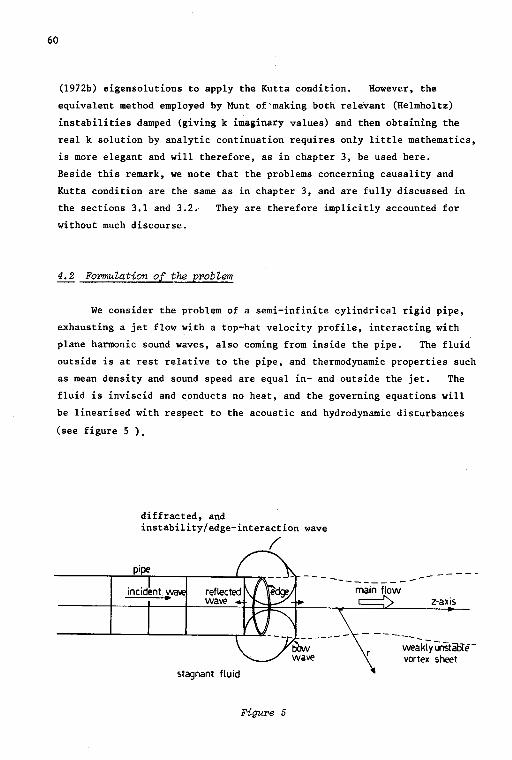
60

(1972b) eigensolutions to apply the Kutta condition. However, the

equivalent method employed by Munt of'making both relevant (Helmholtz)

instabilities damped (giving k imaginary values) and then obtaining the

real k solution by analytic continuation requires only little mathematics,

is more elegant and will therefore, as in chapter 3, be used here.

Beside this remark, we note that the problems concerning causality and

Kutta condition are the same as in chapter 3, and are fully discussed in

the sections 3.1 and 3.2. They are therefore implicitly accounted for

without much discourse.

4.2 Fol'171UZation of the probZem

We consider the problem of a semi-infinite cylindrical rigid pipe,

exhausting a jet flow with a top-hat velocity profile, interacting with

plane harmonie sound waves, also coming from inside the pipe. The fluid

outside is at rest relative to the pipe, and thermodynamic properties such

as mean density and sound speed are equal in- and outside the jet. The

fluid is inviscid and conducts no heat, and the governing equations will

be linearised with respect to the acoustic and hydrodynamic disturbances

(see figure 5 ).

diffracted, and instability/edge-interaction wave

(

---------z-axis

---- - -----we~iY lÏiStäbTê-vortex sheet

stagnant fluid

Figure 5

The explicit analytic result derived finally is an aymptotic series

expansion, for small Strouhal number, of the axial velocity and the

61

pressure inside the flow, and of the pressure far from the jet.

use the terminology of Munt with a few obvious simplifications.

We shall

Make the problem dimensionless in the following way:

velocities are scaled on the undisturbed jet velocity U, to get

(1 + u,v,w) and (u,v,w) in- and outside the jet respectively;

density is scaled on the mean density p0

, to get 1 + p

lengths are scaled on the radius of the pape jD

time on !D/U and

pressure on P u2 0

2 -1 to get p 0

(p 0

U ) + p , where p 0

is the mean pressure,

The dimensionless sound speed will be denoted by l/M ,

is the Machnumber and c0

the (mean) sound speed; M

where M = U/c 0

is supposed less

than one. As the regions of non-zero vorticity are confined to surfaces

we may introduce ~ , the potential of the velocity disturbances, this

existing everywhere except at the pipe - and jet surface. Here the

required values must be understood as the appropriate limits. Introduce

cylindrical po lar coordinates (r,8 ,z) in such a way that r = 1 , z ~ O

describes the cylinder surface and r = 1, z ~ 0 the undisturbed vortex

sheet separating the jet flow from the ambient stagnant fluid.

For the primary wave ~o , coming from inside the pipe, we take

~ (r,e,z,t) 0

~ (z) exp ( iwt) 0

exp (- i ~ z + i w t) ( r < 1) 2rr l+M

(4.2.1) 0 (r > 1)

where k = w M. If an incident pressure of amplitude unity is preferred,

the resulting solution should be multiplied by 2 rri (l+M)/w . Note that

the dimensionless frequency w is equal to the Strouhal number rr f D/U ,

where f is the real frequency; the dimensionless wavenumber k = w M is

equal to the Helmholtz number We postulate some natural

62

damping mechanism, not actually included in the model, which prevents other

time and angle 8 dependence to óccur than generated by the primary wave.

So in our case the time dependence appears in the solution as the factor

exp (iwt) which will be suppressed throughout, and moreover the solution

is independent of a • Anticipating the use of Fourier transforms, it is

advantageous to write $ as the sum of the primary wave $0

and a wave

W , accounting for the whole set of effects produced by the interaction of

$0

with the pipe edge and the vortex sheet, such as diffraction,

transmission, reflection, refraction, vortex shedding and instability

generation. If we add, temporarily, enough artificial damping, by means

of a non-zero imaginary part of wavenumber k , to make the instabilities

decreasing, W is square integrable, so its Fourier transform exists (as an

ordinary function). After having found the solution for complex k we

obtain the required solution with real k by analytic continuation of the

solution as a function of k See also section 3. 2 •

Taking into account the above-mentioned considerations and applying

the acoustic approximation P = M2p , the equations, with boundary

conditions, for W(r,z) = $ - $0

and p are (the index z or r means

dif f erentiation with respect to that variable)

Wzz + .!. (r W ) + k2 W - 2 ik MW r rr z 0 r < 1 , (4.2.2)

w zz +

1 (r W ) + k2 w

r rr 0 ' r > 1 , (4.2.3)

p w z r < 1 , (4.2.4)

p r > 1 . (4.2.5)

From the rigidity of the cylinder it follows that

0 z ~ 0 ' (4.2.6)

while from the continuity of pressure across the vortex sheet it follows

that

ikl/J(l+O,z) - ikl/J(l-O,z) - M l/!2(1-0,z) 1. k ( )

l+M q, o 2 '

The vortex sheet is a material surface, so that if

r 1 + h(z) exp(iw t) for z > 0

is the position of the vortex sheet, it follows that

i w h(z)

iw h(z) + h (z) z

z > 0

z > 0 •

63

no. (4.2.7)

(4. 2 .8)

(4.2.9)

(4.2.10)

At the edge of the cylinder we impose the Kutta condition of smoothness

h(z) = O(z312

) (z t 0) . (4. 2 .11)

The field of ljJ is radiating outwards, therefore

k 1 ki exp ( - i 6 ) 0 < 6 < 1T • (4.2.12)

4.3 Formal solution

Following Munt we introduce

the Fourier transf orm of l/J

S(r,s) J ljJ (r,z) exp(- s z)dz , s complex (4.3.1)

in the complex s-plane the halfplanes

the © plane Re s > - M sin l+M

the G plane Re s < !ki sin 6 '

l (4.3.2)

where the common strip is called the strip of overlap; the indices + and

64

- will denote regularity in the respactive halfplanes;

the Fourier transform of h

F+(s) = J h(z) exp(- s z) dz

0

(4.3.3)

the Fourier transform of the pressure difference across the pipesurf ace as

far as it is induced by ijl

G_(s) ( [ikljl(l+O,z) - ikljl(l-0,z) - Mwz(l-0,z)]exp(-sz) dz

and the complex functions

1 À

1(s) = (s2 - (ik+Ms)2) 2

+ Àl (s) ((1 + M) s

À 2 (s) (s2 + k2) ! + À 2 (s)

+ ik)!

À;(s)

+ À2(s) (s +ik)! , À; (s)

where

ÀÎ (s) ((1 - M) s - i k~

where

(s-ik)!.

(4.3.4)

(4.3.5)

Branch cuts run from ik and ik/ (1-M) to ik "' , and from -ik and

-ik/(l+M) to -ik"' respectively.

by

The appropriate branches are def ined

! J kJ 2 exp ( i ! 11 - i ! ê ) , and

À~(O) 1

JkJ 2 exp(-i ! 11 - i ! ö) • (The same as (3.4.5)).

Introduction of (4.3.1) in (4.2.2) and (4.2.3), and application of the

boundary conditions leads to

tl (r, s)

tl(r,s)

(ik+ Ms) F (s) +

ikF (s) + H <2> {À (s)r)

M À2 (s) Hp) (À2

(s)) 0 2

r < 1

) (4.3.6)

r > 1

and the functional equation

( ) + _!__ i_l;_ 1 G s 2Tr l+M ik

s + l+M

k3 F+{s)x(s)

M Àl {s) À2

{s)

65

(4.3.7)

all valid for s in the strip of overlap. The function x, defined by

X (s) - (ik + Ms) 2 À

2{s) J

0(À

1{s))

k3 Jl (Àl (s))

À (s) H(Z)(À2

(s)) 1 0 (4.3.8)

is crucial in the analysis. The dispersion relation of the possible waves

in the system is given by x(s) = 0 . The functions Jn and H~2 ) are

the n-th order Bessel function of the first kind, and the n-th order Hankel

function of the second kind (Watson (1966)).

Equation (4.3.7) will be solved by means of the Wiener-Hopf technique

(see Noble (1958), or section 3.4 right after (3.4.10)). The first thing

to do, to prepare the splitting of (4.3. 7) is to write x = x+I x _

where and x_ are not only regular but also non-zero in their

respective halfplanes. So the zeros of x play an important róle and

must be treated carefully. According to Munt's analysis (partially

relying on a numerical search) there are, from the infinity of poles and

zeros, just two zeros, denoted by s and 0

plane into the other for varying complex k

which move from one half-

Therefore it is convenient

to write (slightly different from Munt, to be uniform with chapter 3)

1 x{s)= --(s- s ) (s- s3) µ (s).

k2 0 (4. 3. 9)

We note that in the case of small w (therefore small k ) the

behaviour of the zeros will be obvious, and we do not really need Munt's

numerical work. At the end of this section we shall summarise the

general properties of the zeros, but of these it is now important to note

that when

66

I.

II.

the

is in the neighbourhood of 0 , s0

is not an element of

e plane ' and s3 is not an element of the ® plane,

is in the neighbourhood of

elements of the ® plane.

w, both s0

and s3

are not

A splitting il = (l+!(l_ with µ+ and µ regular and non-zero in

their halfplanes, can be made now independent of k in general behaviour,

from which the split functions X+ and x follow by inspection with the

aid of (4.3.10). Explicit expressions of µ± are always possible (see

(3.5.1)) but we do not need them here. Using the splittings of +

and +

and noting that - ik/ (l+M) is element Àl = Àl Àl À2=À2À2 ' not an

of the ® plane, we can establish the splitting of (4.3. 7) for the two

cases of (4.3.10). As was anticipated, case I yields the stable

solution, which cannot satisfy the Kutta condition, so we shall ignore

this. Case II gives

G (s) À~(s) À; (s) µ (s) + -

ik [À~ (s) À; (s) ' (s) - -ik - -ik ' -ik ] 2iT l+M. ----rk µ - Àl (l+M) À2(l+M) µ_ (l+M)

s + l+M

1 ik 1 - 2w 1 +M ik

s + l+M (4. 3 .11)

The equality holds in the strip; the left hand side is regular in the

e plane, the right hand side is regular in the ® plane, and so they

define together an entire function E(s) . To determine this function we

use some well-known results (the "Abelian theorems", Noble (1958), page 36)

which relate the behaviour of a function near the origin to the behaviour

of its Fourier transform near infinity. From the Kutta condition (4.2.11)

it follows that F+(s) = O(s-512 ) when Is! ~ oo in the ® plane.

Secondly, the force on the pipe surf ace is finite, so the pressure

dif ference is at least integrable, i.e. O(z-l-q) for z t 0 with q < 0,

which gives G (s) = O(sq) when - 1 si ~ 00 in the e plane. Furthermore,

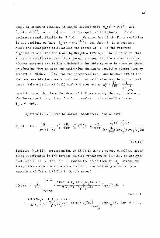
67

' l applyjng standard methods, it can be deduced that µ+(s) = O(s 2

) and

µ (s) = O(s-!) when 1 si ~ in the respective halfplanes. These

estimates result finally in E - 0 . We note that if the Kutta condition

is not applied, we have F+(s) O(s-312

) and then E is a constant.

After the subsequent calculations the factor of E is the relevant

eigensolution of the set found by Crighton (1972b). In relation to this

it is now easily seen that the theorem, stating that there does not exist

without external excitation a Helmholtz instability wave in a vertex sheet

originating from an edge and satisfying the Kutta condition (formulated by

Bechert & Michel (1975) for the incompressible - and by Howe (1976) for

the compressible two-dimensional case), is valid also for the cylindrical 1 ik 1

case: 2n l+M -------riZ

s + l+M

take equation (4.3.11) with the sourceterm

equal to zero, then from the above it fellows readily that application of

the Kutta condition, i.e. E = 0 , results in the trivial solution

F+ = 0 only.

Equation (4.3.11) can be solved immediately, and we have

+ i

(4.3.12)

Equation (4.3.12), corresponding to (5.3) in Munt's paper, supplies, after

being substituted in the inverse Fourier transform of (4.3.6), by analytic

continuation in k for 6 ~ O (where the transition of s across the 0

integration contour must be accounted for) the following solution (see

equations (5.7a) and (5.7b) in Munt's paper)

ij; (r, z) 1

2ni

ico-o

J -ico+o

(ik+ Ms)F + (s) J0

(),1

(s) r) ----,--,,----0----,-,----,-'7-- exp ( s z) d s

M Àl (s) J1

(À1

(s)) +

F+ (s) 1 exp(s0

z) , for - s=s

0

(4.3.13)

r < 1 ,

68

ioo-o

1jl (r, z) 1

2î!i J ik F+(s) H!

2)(1,

2(s)r)

M À2

(s) H(Z) (À (s)) exp (sz)ds +

-ioo+o 1 2

(4.3.14)

for r > 1.

The branchcuts coincide now (for real k) with the imaginary axis, while

the contour of integration runs for negative imaginary arguments on the

right side, and for positive imaginary arguments on the left side of the

cuts. We shall call the integrals of (4.3.13) and (4.3.14) the stable

part of the solution, and the remaining exponentials the instability part.

In the next section we shall calculate the far field of the pressure

p - iw1jl '

and the complete field inside the jet of the pressure -1

i w 1jl- and the axial velocity p - iw (l+M) cj> - 1/iz -1 0

cj>z = - i k(l+M) cj>0

+ 1"z For the outer field it is irrelevant whether

pressure, velocity, or whatever variable is taken. Inside the jet,

however, we have to be very careful with differentiating the asymptotic

expansion it changes the order of the terms and thus the order of

magnitude of the error term. It can easily be deduced from the final

expression that in cj> the diffraction effects are of the order of

magnitude of the error term, while in cj>zz the diffraction effects are

part of the leading order term, together with the primary and the

instability wave. The basic reason for this is that essentially two

length scales are involved: the acoustic and hydrodynamic wavelengths

2îl/k and 2î!M/k = 2î!/w , respectively, on the one hand, and the much

smaller pipe radius ( = 1) on the other. The instability wave and the

reflected and transmitted primary waves are longitudinal and propagating

along the z-axis with only slow variations in z and therefore disappear

w'ith differentiation with respect to z • The diffraction waves, however,

are pointing in all directions and give, via reflections against the

pipesurface, order one variations in the z-direction, which preserve the

order of magnitude of the diffraction waves after differentiation.

This completes the derivation of a formal solution to the problem.

Before proceeding with an explicit approximation, we sum up the general

properties of the zeros of x .

As discussed extensively by Morgan (1975) and extended by Munt with

numerical examples of representative cases, the zeros of x are

s and 0

correspondi.1g to the increasing and decreasing HelmholtZ

instability,

69

and near the hranch points, for k + 0 exponentially close to

s = ±ik

an infinite sequence of ze ros near the line

Im s = kM/ (1-M2 ) in the G plane,

an infinite sequence of ze ros near the line

Im s = kM/(l-M2 ) in the e plane

The characteristic behaviour of the zeros as a function of k is (Munt,

p.621), that s0

and s3

are more or less linear ink and the others are

rather insensitive to changes of k they never move to another halfplane

For the limit case w + 0 (sok+ 0) , which we will discuss, this is also

readily clear from the explicit approximations. Of these zeros, s0

, Ç+

and a1

, a2

, ... , with positive real parts, are all candidates to

represent instability waves. However, ç+ and most of the a1

, a2

, ...

correspond to incoming waves and must therefore be rejected. For M small

enough and k not too small, there is a finite number a1

, ... , aN with

negative imaginary part, and so corresponding to outgoing waves, as Crow &

Champagne (1971) and Lee & Jones (1973) found. However, the calculations

show that only s0

and none of the a1

, ... , aN appear as instability

waves. Of course, we are relying here on some uniqueness assumption for

the solution. The physical mechanism for this is not clear as yet.

possible conjecture might be, that the waves corresponding to a1

,

A

a N

cannot be connected to the pipe edge without vanishing everywhere, and are,

as they do occur in the infinite vortex sheet model, only appearing in a too

far simplified problem. They may occur then, in reality, far from the edg~

hut probably do not because of the thick and turbulent mixing layer. No te

that ai and ç± are rather insensitive to k and only scale upon the

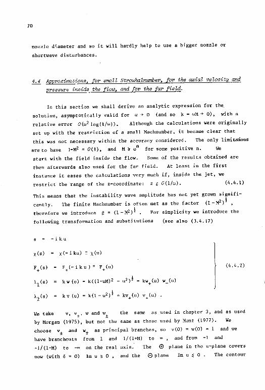
70

nozzle dfameter and so it will hardly help to use a bigger nozzle or

shortwave disturbances.

4.4 Approximations, [or small Strouhalnumber, [or the axial veloaity and

pressure inside the flow, and [or the [ar field.

In this section we shall derive an analytic expression for the

solution, asymptotically valid for w + O (and so k = wM + 0), with a

relative error O(w2 log(l/w)). Although the calculations were originally

set up with the restriction of a small Machnumber, it became clear that

this was not necessary within the accuracy considered. The only limitati.ons

are to have 1-M2 = 0(1), and M :t' wn for some positive n. We

start with the field inside the flow. Some of the results obtained are

then afterwards also used for the far field. At least in the first

instance it eases the calculations very much if, inside the jet, we

restrict the range of the z-coordinate: z :; 0 (l/w). (4.4.1)

This means that the instability wave amplitude has not yet grown signifi­!

cantly. The finite Machnumber is often met as the factor (l-M2 )2

,

therefore we introduce S = (1 - M2) ! . For simplicity we introduce the

following transformation and substitutions (see also (3.4.17)

s -iku

x(s) x(-iku)=x(u)

F+(-iku)= F+(u) (4.4.2)

k w (u) k((l-uM)2 - u2)! = kw+(u) w_(u)

k v (u)

We take v, v ±. w and w the same ±

as used in chapter 3, and as used

by Morgan (1975), but not the same as those used by Munt (1977). We

choose v± and w± as principal branches, so v(O) = w(O) = 1 and we

have branchcuts from and l/(l+M) to and from -1 and

-1/(1-M) to on the real axis. The <±> plane in the u-plane covers

now (with cS = 0) Im u 'il 0 '

and the e plane Im u ~ 0 The contour

71

of integration runs from + 00 above the branch cuts to underneath

the branch cuts, crossing the real axis somewhere between -1 and 1/ (l+M).

As might be expected, the behaviour of the integrands of (4.3.13,14)

is not uniform on the contour of integration for w ~ 0 . If we stick to

the relative error of O(w2 log(l/w)), however, it is almost uniform, apart

from a few points which can be avoided, using section 3.5 under the

condition (4.4.1). Otherwise they must be treated separately (section4.5).

The real prnblem in approximating the integrands is the approximation of

So we shall start with this. We have

x(u) J (kw(u))

(1 - uM) 2 v(u) 0 - w(u)

J1

(kw(u))

H( 2)(kv(u)) 0

The expansions for small arguments of the Bessel functions give

(Gradshteyn & Ryzhik (1965))

J (z) 0

Jl (z)

H( 2 ) (z) 0

2 (1 + 0(22)) z

- z log (j i z expy)(l + O(z2 log z)) ,

)

(4.4.3)

(4.4.4)

(where y = 0.5772 ... Euler's constant, and the principal branch of log

is taken), and for large argument, when lul ~ 0(1/k) on the contour

J (k w (u)) I (Bku) 0 sgn(Im u) 0 + O(wM2 ) 0 ( 1), ----

J1

(kw(u)) r1

(Bku)

(4.4.5)

H( 2 )(kv(u)) K (ki ui) 0 0

0(1) ' Hi

2) (k v(u)) - 1

Kl (klul)

where I and K are modified Bessel functions of the first and second n n

kind. Note that 1

w(u)/B v(u) ~ (-u2) 2 - i sgn (Im u) u that on the contour Im u

72

changes its sign together with Re u , that In/Im , K0

/K1+ 1 for

lul + oo on the contour, and that In has no zeros outside the origin, and

Kn has no positive zeros or singularities (Watson (1966)). Using (4.4.4)

we can find approximations to the most important zeros u 0

i s /k 0

ul = i s3/k viz

1 (1 + O(w logi ..!.) = ..!.o + i ! II wlog! ..!.)(1· + O(w log-! 1 )

u M ;». 0 w . M w

1 (1 + O(wlog! -b> = ..!.o - i ! 12 wlogi ..!.) (1 + 0( w log-! ..!.)) • ul = -M M w w

and

(4.4.6)

In this section, we will only use the rougher approximations. However,

these have zero imaginary part. To distinguish them and to realise that

the contour of integration runs between them, and that u0

is an element

of the G> plane and ul of the e plane' it is important to refer to

the imaginary part of the exact u0

and u1 . We shall do so by writing

1 i. 0 u -+ 0 M

1 i. 0 ul M l (4.4. 7)

Using (4.4.4,5,7), and after analyzing the regions near u = +I and u = -1

in particular, it can be shown that an approximation to x is given by

M2 (u 1 M

J (kw(u)) i. O)(u - ..!. + i. 0) v(u) _o ___ _

M J1

(kw(u))

with x x (1 + O(w2 log(l/w)) everywhere, except in the regions

± 1 + o<..l. 0(1) (loosely speaking)

} u exp(- --))

' k2 k2M

1 (1 + O(w log! l)) u "M w

(4.4.8)

(4.4.9)

Outside these regions, we know from section 3.5 that X+ and x , where

~ = x+/x_ , approximate X+ and X_·

decomposition of J0

and J1

Using the infinite product

73

J (z) 0

z2 ll (1 - --)

n=l ·2

) 3o,n

(4.4.10)

1 z2 2

z ll (1 - -.2-) n=l 31 ,n

where jo,n' jl, n is the n-th zero of J o' Jl (Watson (1966)), we can

construct the following expressions for x+ and x

M j2 62 !

v + (u) u + +- (~- 1)

j x+ Cul (u -~- i.O) (u -~+ i.O)

s2 s2 k2 ~ w+(u)

ll j2 62 ! jo,n n=l M i ( l ,n u + +- - 1) s2 s2 k2

(4. 4 .11)

j2 62 1 M i 2

(u) j u + (~- 1)

k w s2 s2 k2 (4.4.12) x (u) -

ll .....2..>E. 2M2 v (u) n=l \,n M i j2 62 !

u + (~ - 1) sz s2 k2

Note that these are of algebraic behaviour at infinity.

If, following the ideas presented in section 3.5, we deform the

integration path for the integral expressions of q, and z

p in to the one

described in figure 6 '

we can use approximations (4.4 .11) and (4.4.12).

The new path consists of the old one with an indentation around u = l/M

forming a semi-circle in the (tl plane with a radius many times -1 l

w M log' (l/w), and indentations around u = +I and u = -1 with radii

largely depending on M. When M is of order 1, the radii may be of the

order of some positive power of w ' whereas for smaller M they may be

exponentially small. In fact, the regions near u = +I and u = -1 are

of a difficult type. We have an infini te, nested sequence of regions of

non-uniformity there. HoT'lever, they can all be avoided, and we shall not

discuss this point any further.

74

uet

.~

\ \, .Ut,/

region èr rm-oofamity

·Figure 6

The pole u = u0

is crossed during the deformation, so the instability

parts of (4.3. 13) and (4.3. 14) are included then in the integral.

Note that we need the restriction (4.4.1), i.e. z ~ 0(1/w).

Approximated as in (4.4.7), u0

yields for z > 0 an error of

O(zw2log!!) in the argument of the instability wave, and hence, when w

z ~ 00 , an exponentially large error in its amplitude. It is a subtle

point that it is necessary only to take z ~ 0(1/w) , rather than

z < O(log! (l/w)). Considering only the influence of u0

, we would expect

the strenger restriction. However, is close to and almost its

complex conjugate, i.e. u0

~ ui giving rise to a sart of interference

between the increasing (u0

) and decreasing (u1

) wave. The resuü is

O(w2 log!(l/w)z}. a relative error of O(w4 log(l/w) z ) , instead of

Illustrative for these points are the following model integrals

( where a corresponds to l/M, and € to jlïwM""llog!(l/w) ):

_ ____,_( u_-_a_),__e_x_.p_,(~-:""i~k-=u=-z ,_) __ du

(u-a-iE)(u-a+iE)(u2+1)

1 f (u-a)2exp(-ikuz) -- du 2ni ~(u-a-iE)(u-a+iE)(u2 +1)

75

for ~z and

for p

where the "c" in the integral sign denotes an indented integration path.

On the other hand, examination of the expression for h ,

h(z) = 2kn f F+(u) exp(-:ikuz)du - ik[ (u-u )F (u)] exp(-iku0

z) , . 0 +

u=u 0

reveals that h contains in the leading order the factor l/(u0-u

1),

which is infinite when we use approximation (4.4.7). Still h is finite

when w ~ O , because the numerator multiplying this factor approaches

zero at the same rate. When we take care, the present approximation is

applicable, but we shall not evaluate this here.

After substitution of (4.3.12) for F+ and -iku for s , we

arrive at the following expression for the axial velocity inside the pipe

and the jet

~ (r, z) z

ik exp(-i_!_z) - 2n(l+M) l+M

+ ikM ( 1 ) 2n(l+M) w_ l+M

00+i.o

2;i f - 00-i.o

(u_l_)u J (krw(u)) v (u) w (u) exp(-ikuz) __ M __ ~o __ ~ __ + ___ + ________ du .

w(u)(u--1-) J

1(kw(u))x+(u) l+M

(4.4.13)

Substitution of (4.4.10), (4.4.11) and (4.4.12) gives <ignoring the terms

irrelevant in the present approximation)

76

where CJ

ik -ik iw exp(l+M z) +

7r(l+M)f32 (1 . k )

- 1 j3 CJ 27r (l+M)

u J 0

(krw(u) )exp ( -ikuz)

(u -.!.) (u --1-)(u +-1-) M l+M 1-M

+ O(k w2 log.!.) , w

l .,]_ - -. l_ n=l Jo,n Jl,n

0.2554 ...

(4.4.14)

(4.4.15)

When z > 0 we can close the contour via a large semi-circle in the lower

halfplane, and when z < 0 in the upper halfplane, and obtain in the same

accuracy

z > 0 ik ( 1-M l - 7r(l+M) exp -iw(z-(l+M) CJ)]

(4.4.16)

z < 0 ik [ - 27r (1 +M) exp

wk z 2 1 - 7r(l+M)f3 ;<r,8) + O(k w log;>, (4.4.17)

where L0

and Ll are given by

77

J (r j o ,rn ) exp (-z 'j )

i;0(r,z') I 0 o,m (4.4.18)

j j j m=l j (1 + .o,m) Tl (1 - . o,m) (l + .o'm)

o,m J l,m n=l Jo,n J l ,n

n#m

Jo(r jl ) exp(z' j ) i:

1 (r, z') I m l,m ( 4. 4. 19) j j j

m=l j l,m (1 + .1,m) Tl (1 + .l,m)(l _ . l ,m)

Jo,m n=l Jo,n J l ,n n#m

Note that l:0

and i:1

are exponentially small for z' ~ 00 and - 00 respectively.

The analogous result for the pressure p is

p(r,z) iw - 2TI(l+M)

ikM - 2TI (1 +M)

00 +i.o

2~i 1

-ik exp(l+M z)

1 2 . (u-M) J

0(krw(u)) v+(u) w+(u) exp(-1kuz)

- 00-i.o w(u) (u --1-) Jl(kw(u)) x+(u) l+M

Substitution of (4.4.10, 11, 12) yields

du .

(4. 4. 20)

78

p(r,z) iw

- 211(l+M) -ik

exp<l+M z) iw

11 (1 +M) B2 (1-i!.c )·

B J

J0

(krw(u)) exp(-ikuz)

(u +-1-) (u - _l_) 1-M l+M

+ O(w 3 log .!.) , w

and so for

z > 0 p(r,z) wk l: ( z) + 0 (w 3 log .!.) 11(l+M)B o r,S w

and for

z < 0 p(r,z)

+ ~ i: 1 (r,~) + O(w 3 log -w1) 11 (1 +M) B "'

(4.4.21)

(4.4.22)

(4.4.23)

As is usual in duet acoustics, the incident primary wave is cancelled

outside the pipe (z > O); a conclusion is that the presence of the vortex

sheet is not enough to keep more inside the jet than a part of the

diffracted wave.

Outside the pipe the presence of the flow îs obviously marked by the

instability wave. Inside, however, we also observe striking differences

from the no-flow case although these are not as pronounced as the instabi-

lity wave. If we def ine the reflexion coef f icient R as the ratio of the

coeff icients of incident and reflected primary wave in pressure form, we

have from (4.4.23)

79

R c

- exp ( - 2 i k s3) instead of - exp (- 2 ik ,q , (4.4.24)

and an end correction (phase shift due to the reflection)

instead of i 0.6133 ... (Noble (1958), p.115,138). (4.4.25)

For a proper understanding of these results, it is important to note, that

(after performing analogous calculations as above) the pressure wave far

upstream inside the pipe, for the case in which no vorticity is shed from

the edge, is given by

So now the reflection coefficient has IRI = (l+M)/(1-M) , instead of

unity, although, on the other hand, the end correction is still S CJ . As

a conclusion we have that the Kutta condition does not affect the end

correction (at least, when compared with the no-shed-vorticity-case), but

does change the reflection coefficient. The difference is probably best

expressed by considering the power flux. According to Blokhintsev (see

Candel (1975)), the net power transmitted along the tube toward the exit

is (modulo some dimensional constants) given by P "-' (l+M)2 p~ - (l-M) 2 p:_ ,

where and P_ are the amplitudes of the incident and reflected

primary wave. We see that when no vorticity is shed, no power (in the

limit k + 0) is transmitted, in contrast to the Kutta condition case,

where P "-' 4M /(l+M) 2.

A surprising result is illustrated by taking the limit M + 0 of the

end correction, giving CJ, which turns out to be different from that of

the no flow case (see (4,4.25)). As the value of w is restricted, this

limit yields incompressible flow. Only when M + 0 is taken first with

k = w M fixed, and then k + 0 , we would have the no flow case, The

double limit (M,k) + (O,O) is not uniform, which can also be seen by

comparing x (4.4.3) with x (4.4.8) for M = 0 and finite k . The

present problem is thus seen to provide an example of a non trivial

interaction of incompressible flow (at first sight acoustically

equivalent to stagnant flow) with sound waves.

80

An interesting feature, revealed by (4.4.22), is that on the interval

0 ~ z ~ 0(1/w) no instability wave can be observed by pressure measure-

ments. Almost all the flow energy is merely being convected. The

instability wave must be considered as a moving velocity - (vorticity)

distribution, fixed in the moving frame of the jetflow, comparable with the

undulating wake behind a flat plate, discussed in chapter 2. From

Bernoulli's law, we can

lity wave has the form

pressure p = - $t - $x

expect in our case, where the increasing instabi­' $ "' exp [iwt-iw (1 +i ! 12 w log~ (l/w)) z] • that the

is negligible on the interval 0 < z < O(log!(l/w)).

The bonus, however, is an interference of the increasing.and decreasing

Helmholtz instability waves (corresponding to u 0

and u1), resulting in

a cancellation of the corresponding pressure even on the interval

0 ~ z ~ 0(1/w)

The vanishing of the pressure perturbations in the jet flow on the interval

1 << z ~ 0(1/w) (see (4.4.22)) can also be seen in the following context.

When wè compa.re the energy fluxes of the acoustic and hydrodynamic

disturbances in the flow far upstream in.side, and downstream outside the

pipe (Goldstein (1976), p. 41), we see that these are equal for vanishing

Strouhal number. Noting'that the energy in the jet flow is mainly kinetic

(compare (4.4. 16) with (4.4.22) for z>O), we can conclude that almost all

of the incident acoustic energy is transferred into the kinetic energy of

the shed vortices. This energy conversion is essentially the mechanism,

which Howe (1978) showed to be responsible for the attenuation of the

radiated sound power in the low frequency range, observed by Bechert,

Michel & Pfizenmaier (1977).

The important constant defined ( .-) Jo,n

(using Watson (1966) table VII,p. 748 , and

careful summation of the quantities

page 506), to find

c3

0.25538± 0.00001

An integral representation is

lo~[!xI0 (x)/I1 (x)] d~, x 0

to be compared with the representation

by (4.4. IS), is found by -1

- j 1,n) on a pocket calculator

the asymptotic expression at

(4. 4. 26)

1

J 0

1 dx log (2K

1 (x) I 1 (x)_ 2

x 0.6133,

which defines the end-correction in the classical no-flow case at low

81

Helmholtz numbers. The rather rough approximation (Watson (1966),p.506)

. (n - .!:.) 11 Jo,n 4

(4. 4. 27)

j (n + .!:.) 11 ' l ,n 4

only correct for large n, gives the promising re sult CJ = 4/11 - 1 = 0.273 ,

which is only 7% off. Using (4.4.27) in l: and l: 1 0 gives US the

opportunity to express the solution on the axis (r = 0) in quore or less)

elementary functions. We obtain then

~{-exp(-11z'),2,i (4.4.28)

+ 2 log 2 11 2 2

cosh(j 11 z') - /2

cosh(l 11z') + /2

4 arctg{ /2 sinh(l n z')} , TI2

i:1

(0,z') 2 1 12 5

<!> { - exp ( TI z') , 5 2 - ex:i(

4nz') 2.4 TI 112

812 exp(j TI z') 2

log 2 cosh(jnz') - /2

+ -- + TI2 TI2 2 cosh(jnz') + /2

4 arctg{/2 sinh(l 11 z')} , (4.4.29)

where <!> is Lerch's transcendent (Gradshteyn & Ryzhik (1965) ,(9.55)),

defined by n

q,(z, s, v) I _z_s n=O(n+v)'

( 1z1 < 1' v 1 0, -1' ... ) .

In appendix 6.2 we give sorne properties of

exp (vy) <J>{-exp(y),2,v} •

82

Using (6.2.2) we obtain, within approximation (4.4.27),

for 1z1 « (both z ;o 0 and z .:: 0 )

ik wk - 1l(i+M) - 1l(l+M)S (0.12 + 0.27M + (0.33 - M2) ~ + O(z2)] ,(4.4.30)

p(O,z) 110 ~~)S [o. 39 - 0.67 ~ + O(z2)] • (4.4.31)

Usually, the amplitude of pressure perturbations is presented in decibels.

Near z = 0 we have from (4.4.31) ( * quantities are dimensional ,

p;ef is some reference level)

_L _ 67 2z* 30 z* 20 log10 * - const. - 20 log 10 (e)39 öj) = const. - 0 i)•

Pref " P

(4.4.32)

Observe that the slope is negative. Here, near the pipe exit, we have only

the decreasing amplitude of the diffracted wave, because in the pressure

the instability waves are effectively absent, as we noted before.

Finally we will treat the far field outside the jet. The expressions

for x± we have now allow us to calculate the far field in a relatively

simple way. If we ignore the bow wave and the instability wave (which are

irrelevant far downstream, and would need much additional calculation) we

have, with the aid of the method of stationary phase applied to (4.3.14),

following the usual steps (Noble (1958)), that

1

(1 - M cosi';) 2 ik exp (-ikr) 411.

r

for kr ~ oo ,where z = r cos ~ , r = r sin ~,and O < ~ < 11 • To

(4.4.33)

make possible a proper comparison with the no-flow case, we have here

normalized the amplitude of the incident wave so that the incident wave

power is independent of M (i.e. instead of ~o we have taken (l+M) ~ 0 ),

From Noble (1958, p.115,138) we can compare with the classica! no-flow

solution (where the same power is incident along the pipe)

83

exp(-ikr) for kr ~ oo

r

The difference is clearly just a squared Doppler factor, one of which is

associated with the very slowly growing instability wave and the ether with

the decaying, When no vorticity is shed, we would have only the decaying

wave and thus only one Doppler factor.

4,5 Extensions downstream

The aim of this section is to extend the results inside the jet

downstream to z > 0(1/w) • Restriction (4.4.1) of z ~ 0(1/w) was -1

necessary when we employed the simple approximations u0

~ M and

u1

~ M-l , Obviously, we could have had a larger region of validity of

the previous solutions right from the start by using better approximations

However, this would have increased the complexity of the

formulae very much, while the present solution yields virtually all the

important conclusions already. Therefore it improves the clarity to defer

a refinement of the approximations to a later section, This is even more

worthwhile, because in the region z >, 0(1/w) the solution behaves much

more simply than further upstream, and so we only have to consider this

region separately. To see this, note the following: there is no primary

wave outside the pipe, the diffracted wave has an order-one exponential

decrease, so we have for very large z only the u0-instability wave left

over, and for z >, 0(1/w) the u0

- and u1-waves. Therefore it suffices,

to complete the analysis for all z , to calculate the contributions from

the poles u 0

and

For this we go back to.section 3,5,

easily deduced that

Using (3.5.4) it is

84

[X+ (u) J (u-u )

o u=u 0

(4.5.1)

- ( ) d ( ) (1 + O(w21ool)). X ul du X ul "'w (4.5.2)

Introducing these into (4.4.13) and (4.4.20) (i.e. $z and p) together

with (4.4.11) and (4.4.12) (i.e. and

possible, the relevant approximation, yields

x_), and applying, where

(note: x'= ~u x

(4.5.3)

[

(u -!)v(u ) o M o . • exp(-1ku z)

u2 x'(u) 0

1 (ul-M)v(ul)

0 0 uf x'(ul)

p(r,z) (4.5.4)

for z >, 0(1/w) and r ~ 1 The connections between the expressions

va lid on z ~ o(l/ w) with the expressions valid on z >, o(l/w) should

be understood as "matching". The range in z we can cover now depends

completely upon the accuracy we have in the approximation for u0

and,

until the decreasing u1

-wave is small, for u1

. So in principle we cai

reach every z . This is not necessary,however, because the thickening

of the real mixing layer limits the applicability of our model, and, after

all, our (linear) model is definitely not valid anymore in the region

where the waving vertex sheet reaches the axis r = 0 .

An example of an approximation for

z-region up to z ~ O(w-2 log!(l/w)) ,

u 0

is

and u1

which extends the

(use (4.4.4))

X (u ) 0

x r l <1 + ··M

(4.5.5)

log(! S ~xpy) + 2 w. log!(~) t -~ {.l.. + 2 log(j S expy)}.j 0 log (-) 0 log 2 cl) S2

w w

with Im t0

> 0 , and

v(ul)w2 1 [ -- -log(-) 2 t 2 + l w(u

1) k w l

(4.5.6)

'ITi+log(jSexpy) l 1 w tl f 1 . }} - 1 + 2wlog C;;;lt 1 ---1 -1~-+2n + 2log(jBexpy)

log C;;;) log 2 <;;;l s 2 0

with Tm t1

< 0 .

Equations (4.5.5) and (4.5.6) give, via a simple algebraic equation, u 1 0

O(w 3log 2 (l/w)) and and u1

with relative errors of

O(w3 log 312 (1/w)) respectively. Moreover, they provide estimates for d du x at u

0 and u1 . Differentiation of (4.5.5,6), and then, finally,

85

substitution in (4.5.3,4) of all the results obtained, yields, respectively,

to leading order

~u x(uo) - ~u x(ul) ~ 2/2 is logi(;)

ij>z(r,z) ~ 2'IT(~~M) [ exp(-iku0

z) + exp(-iku 1z) J , 1

Mw2log2

(1/w) [ J p(r,z) 2/2'IT(l+M) exp(-iku0

) - exp(-iku 1)

(4. 5. 7)

(4. 5. 8)

(4.5.9)

And hence, we obtain for large z (using the same notation as in (4.4.32))

_L- _ 2z* 2 1 1 z* 20 log 10 * - const. + 20 log 10 (e) Im(u

0) k -n- ~ c. + 12.3 w log 2 (-w) D .

Pref (4.5.10)

86

±!.§.. Comparison with ewperiments

As a general remark it should be noted that it is difficult to

compare the calculated sound pressure levels with the measured ones.

Owing to the different resonance characteristics of a real pipe system for

different Mach numbers, we have unknown effective incident wave amplitudes

to scale on. Therefore we shall only consider the variations of the

measured data.

As we pointed out before, the present model was evaluated numerically

by Munt (1977) for the far field, and the agreement with the experiments

of Pinker & Bryce (1976) was very good, We shall compare our results with

Munt's; agreement, if found, implies then innnediately agreement with the

experiments. The far field expression (4.4.33) is, normalized, in

decibels

const. - 40 log 10 (1 - M cos(E;)). (4.6.1)

Representative values obtained from this expression are compared with those

of Munt (Fig. 13 and 14 of Munt) in the following table,

{SPL(900) - SPL(l70D)} {SPL(500) - SPL(l70D)} w 'M Munt, expr.(4.6.1), rel.error Munt, expr.(4.6.1), rel.error

0,27 0.9 10.4 11.0 6 % 24.5 26.0 6 % 0.40 0.6 7.6 8.1 7 % 15.8 16.5 4 % 0.67 0.9 10.1 11.0 9 % 22.7 26.0 15 % 0.80 0.3 4. 1 4.5 10 % 7.8 8.2 5 % 1.00 0.6 7.0 8.1 16 % 15.0 16.5 10 % 2.00 0.3 3.0 4.5 50 % 7. 1 8.2 15 %

where {SPL(;) - SPL(l70D)} denotes the increase of the sound pressure

level in decibels from the value at 1700 to that at ; It is seen that

the present results agree well with those of Munt. Thus the simple

expression (4.6.1) is capable of representing the far field for Strouhal

numbers w right up to a value of one, possibly even two. Another

feature of these calculations is that it is easy to observe the role that

Kutta condition plays in the far field. When this condition is absent, the

factor 40 in (4.6.1) would be 20. Therefore the agreement with the

experiments shows that vortex shedding contributes signific'antly to the

far field.

87

Experiments relevant to the present results inside the flow are

provided by Moore (1977). The expressions for the sound pressure level on

the jet axis (4.4.32) and (4.5.10) show features which are in

qualitative agreement with the observations presented in Fig. 20 of

Moore's paper. The slope near the origin, predicted to be -30/8 , is of

the right order of magnitude, which also confirms the effective absence of

the instability waves immediately downstream from the exit. The positive

slope corresponding to the instability wave further downstream from

the experiments for Strouhal numbers sufficiently below unity is of the

same order of magnitude as that predicted by (4.5.10) ( 12.3 w2log!(l/w)).

We see that in the experiments without flow the behaviour of the pressure

outside the pipe is of completely different character than generally is the

case in the presence of flow, viz. a monotonie decrease. For M sufficiently

small and k not small ( M = O. 15 , k = 0.5, and M = 0.3 , k = 1 .2 ) an

intermediate state is seen, which may be a reflection of the non uniform

limit behaviour when (M,k) + (O,O).

The lack of quantitative agreement is believed to be mainly due to the

finite length of the tube used in the experiments. This causes resonance

effects at low frequencies as can be seen in Moore's figures. Moreover,

the smallest Strouhal number w in these experiments is only 0,5 ,

which may be too large to allow detailed comparison.

4.7 Conclusions

We have calculated for a circular subsonic jet, issuing from a pipe

and perturbed by long sound waves, the axial velocity and pressure inside

the flow, and the far field pressure outside. The Kutta condition is always

applied, except, for the purpose of comparison, in a single case, As in

chapter 3 , also here a causality condition is superfluous. By comparing

with the solution without vortex shedding, the Kutta condition appears to

affect the magnitude of the reflection coefficient, hut not the end

correction. In the far field the regular solution differs from the

singular one in having a squared Doppler factor instead of one. When no

vorticity is shed, practically no power is transmitted out of the tube, and

when the Kutta condition is applied, there is a power loss of O(M),

The limit (M,k) + (0,0) appears to be non-uniform, When M + 0 with

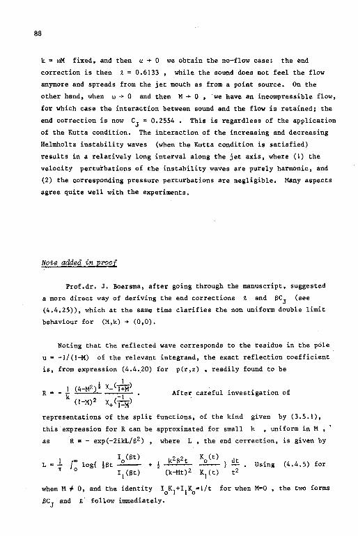
88

k = wM fixed, and then w + O we obtain the no-flow case: the end

correction is then t = 0.6133 , while the sound does not feel the flow

anymore and spreads from the jet mouth as from a point source. On the

other hand, when w + 0 and then M + 0 , 'we have an incompressible flow,

for which case the interaction between sound and the flow is retained; the

end correction is now CJ = 0.2554 , This is regardless of the application

of the Kutta condition, The interaction of the increasing and decreasing

Helmholtz instability waves (when the Kutta condition is satisfied)

results in a relatively long interval along the jet axis, where (1) the

velocity perturbations of the instability waves are purely harmonie, and

(2) the corresponding pressure perturbations are negligible, Hany aspects

agree quite well with the experiments.

Note adàed in proof

Prof.dr. J, Boersma, after going through the manuscript, suggested

a more direct way of deriving the end corrections t and acJ (see

(4.4.25)), which at the same time clarifies the non uniform double limit

behaviour for (M,k) + (0,0),

Noting that the reflected wave corresponds to the residue in the pole

u = -1/(1-M) of the relevant integrand, the exact reflection coefficient

is, from expression (4.4 •. 20) for p(r,z) , readily found to be

1 R = - k

1 (4-M2) ! X_ (J+M) --- -1 (l-M)2 X+(l-M)

After careful investigation of

representations of the split functions, of the kind given by (3.5.1),

this expression for R can be approximated for small k , uniform in M , '

as R • - exp(-2ikL/S2) , where L , the end correction, is given by

L = l f"' log{ 1T 0

I (St) !at - 0

--

11 (13t)

K (t) dt _o __ }

1<1(t) t 2

Using (4.4.5) for

when M + O, and the identity I0K1+I

1K

0=1/t for when M=O , the two forms

acJ and J1; follow immediately.

chapter 5

ACOUSTIC WAVES INTERACTING WITH VISCOUS FLOW NEAR AN

EDGE: APPLICATION OF RESULTS FROM THE TRIPLE DECK THEORY,

5.1 Introduction

89

The acoustic problems, studied until naw, were all simplified in their

neglect of viscosity. In this chapter we shall discuss the consequences

of the introduction of viscosity, especially with respect to the Kutta

condition. Obviously, it must be kept in mind that the inviscid models

of the previous chapters are supposed to apply "almost", i.e. to be

approximations, Therefore the influence of viscosity will be taken as

small. This will imply that we shall ignore the internal friction in a

sound wave, and only consider the boundary layers near the solid body.

Note that the sound wave farms a boundary layer near the wall (the Stokes

layer) as well as the main flow (the Prandtl- boundary layer), and they

may interact. In the end, however, we shall find that only the regions of

the boundary layers near the trailing edge are crucial for tre flow and sound

field interaction, and only these regions are therefore interesting for us.

It is tacitly assumed that the flow is laminar, We try to deal with

rational theories only, and there does not seem to exist any such rational

theory for turbulent flow.

Let us, as a start, confine ourselves to a consideration of a flat

plate of length L , aligned parallel to an incompressible uniform flow

with velocity U and kinematic viscosity v , and with large Reynolds

number Re = UL/v Then it is well-known that along the plate a thin

boundary layer develops (the Basius boundary layer; see for instance Van

Dyke (1975)), eventually giving rise to a wake bebind the plate (the

Goldstein wake; Goldstein (1930)), According to Stewartson (1969) and

Messiter (1970), it appears that the transition from the boundary layer

to the wake is quite a delicate matter. Because of the sudden change in

boundary conditions at· the trailing edge - from zero tangential velocity to

zero stress - the flow in the boundary layer accelerates, which reduces the

90

boundary layer growth, This in its turn causes a small hut sudden

deflection of the main flow streamlines, which induces a singularity of

the mainstream pressure at the trailing edge, This singularity is

smoothed out in a three-layered boundary layer structure (the "triple

deck") around the trailing edge, of dimensionless proportions

0(€3) x 0(E 3) , where Re-l = E8 and E is small. Inside the triple

deck the dimensionless pressure is of order E2 (which is higher than

the surrounding boundary layer-induced pressure perturbations of order

E4 ). This triple deck pressure is a result of the smoothing process. So

an externally generated disturbance will only change this process ,andthus

possibly change the flow, when its corresponding pressure at a distance

from the edge of order E3 is of the same order as the triple deck

pressure (0(E 2)), or larger. We shall, however, not consider the case

of a pressure disturbance much larger than 0(E 2) , because in that case

separation probably starts, for which as yet no theory exists. Although

a pressure disturbance of 0(€2) does modify the triple deck structure,

the resulting outer field is only slightly different from the completely

smooth (Kutta condition) field. Therefore we can conclude that for this

class of disturbances the smooth outer solution adopted in previous

chapters is valid on a rational basis. All these observations,

essentially supplying a rational basis for the smoothing processes at the

trailing edge and leading to an edge singularity condition for the

inviscid outer solution, are generalizations of several deeply studies

examples, We have, for instance, the problem of a flat plate at

incidence in steady incompressible flow (Brown & Stewartson (1970)) and

in steady supersonic flow (Daniels (1974)), a rapidly oscillating flat

plate (Brown & Daniels (1975)), and the problems of wedge and cusp shaped

trailing edges (Riley & Stewartson (1969)), although these last two fall

slightly outside the scope of the form of Kutta condition relevant here,

In addition to these more or less obvious variants of the flat plate

trailing edge problem, the triple deck notion appears to provide an

understanding of many separation problems of all kinds (see for instance

Smith (1977)); indeed its first appearance was in fact in a study of

self-induced separation of supersonic flow (Stewartson & Williams (1969)),

In view of the problems studied in chapters 3 and 4 of this thesis, our

special interest is in the separation behind a flat plate trailing edge,

where a uniform flow together with a Blasius boundary layer on the one

91

side and a stagnant flow on the other form a mixing layer behind the plate

edge (Daniels (1977)). A peculiar property here, is that in the

undisturbed case the triple deck structure disappears (in the main order

of the approximation), because the flow can find an easier way to deal

with the pressure singularity. The deflection of the main flow stream-

lines near the trailing edge - the result of the acceleration of the

boundary layer flow behind the plate - is not necessary now. Prandtl's

transposition theorem for the Prandtl boundary layer equations (Rosenhead

(1963,p.211)) implies the possibility of a small shift of the dividing

rreamline (the streamline emanating from the trailing edge) in the

Jirection of the main flow, which suffices to compensate for the

acceleration. This results in an outer flow singularity of only minor

importanc.. In analogy with the airfoil, it is evidently to be expected,

and indeed the case, that an external disturbance, corresponding to a

non dimensional pressure of 0(E 2 ) in the triple deck region, calls the

triple deck structure (modified on the stagnant flow side of course) back

into play. Daniels (1978) studied this case for the Kutta-condition-

outer solution of Orszag & Crow (1970). Although, as Bechert & Michel

(1975) showed, this outer solution (as well as Orszag & Crow's so-called

"rectified Kutta condition"-solution) is not an eigensolution and only

valid with the presence of a very unusual source, Daniels' (1978) viscous

solution is very useful and generally valid, because every other smooth

outer solution behaves, modulo a factor, in the same way in the triple

deck region.

In addition to his calculations concerning disturbance pressure levels

of order c 2 in the triple deck, Daniels found the possibility of a "no

Kutta condition" outer solution in the mixing layer problem with stagnant

flow on the one side. When the perturbation pressure in the triple deck

is sufficiently small, i.e. of order E912

, he showed that the singularity

of the no vorticity shedding solution is not inconsistent with the triple

deck dynamics, and may be smoothed out in the Navier-Stokes region of

dimensions 0(E6) x 0(E6) around the edge. However, as Daniels argues

on more general grounds, the whole point may be irrelevant altogether, and

furthermore the case of even smaller perturbations is &till an open

question, so that we shall, for the present, only note it, and not include

it in our acoustic problems.

92

The aim of the present chapter is to introduce the triple decks into

the acoustic problems of chapters 2 and 3, to prove, for a certain range of

parameters, the validity of the Kutta condition in laminar flow of high

Reynolds number. Further, for some limiting cases, we shall give explicit

expressions for the far-field correction, due to viscosity, to the

inviscid full Kutta condition solution. Although it is not essential

(Brown & Stewartson (1970,p.584)) we shall restrict ourselves to a Mach

number small enough to give in the triple deck incompressible flow to

leading order. Furthermore, we shall choose the Strouhal number

suffîciently high that the Stokes layer has dimensionless thickness 0(E 5),

which is the thickness of the lower deck in the triple deck. These

choices are only for convenience; they permit analytically tractable

problems, and moreover, they allow us to practically repeat the existing

calculations, namely those of Brown & Daniels (1975) for chapter 2 and

those of Daniels (1978) for chapter 3.

Although virtually impossible to prove, it is most likely that order

of magnitude estimates themselves already inform us also about the

validity of the Kutta condition in the cases we will not consider. So we

postulate that when the dimensionless pressure of the smooth outer solution

behaves like p = constant + A( w,M) /r exp (iwt) + O(r) (r ->- 0), the Kutta

condition is valid (in laminar flow of high Reynolds number) when

A(w,M) = O(~) = O(Re-1116), (the constant can be ignored as it does not

contribute to the gradient).. It should be noted that in reality, a

Reynolds number E-S so high that even lË is small, is impossible in a

harmonically disturbed laminar flow. A Blasius boundary layer is

urtstable for Reynolds numbers beyond 6.10 4 , and definitely turbulent for

Reynolds numbers higher than 3.106 (Rinze (1975)). This may even

invalidate the whole triple deck concept for practical applications.

However, there are reasons - besides the better understanding of the

mechanisms - to relax the "high Reynolds number" condition and to give the

asymptotic expressions from triple deck theories at least the benefit of

the doubt. The skin friction coefficient of a flat plate, based solely

on the contributions from the Blasius boundary layer and the triple deck,

appears to coincide with measurements and numerical calculations in an

astonishing way right down to Re = 1 (Jobe & Burggraf (1974) or Veldman

(1976))and is still very good for Re

solution with Dennis & Dunwoody (1966)À

0,1 (compare Veldman's (1976)

As a second example Daniels (1978)

unsteady solution is in good qualitative agreement with the measurements

of Bechert & Pfizenmaier (1975).

We hope to have given a general idea of the relevant aspects of the

triple deck and its modifications, at least sufficient to enable the

reader to follow the applications to our acoustic problems in the next

sections. We shall not consider the different triple deck layers and

subboundary layers in detail. We do not claim to contribute anything

important to the triple deck theory itself, so we think that for those who

are interested in its detailed description, the original literature is

most recommended.

5.2 Formulation of the problems

In the chapters 2 and 3 we considered, for convenience and clarity,

a semi-infinite plate. Obviously we would like to preserve this geometry

in the present viscous problems. However, a careless introduction of

viscosity would rule out the possibility of an inviscid outer solution,

because the influence of the plate would then be felt everywhere,

Therefore, we shall modify the properties of the plate a little with the

rather artificial assumption that the plate is frictionless everywhere,

except for a finite part upstream of and including the trailing edge. The

dimensional length of this part is L; it will be our reference length-

scale when we make the problem non-dimensional. The coordinate axes are

93

chosen in the same way as in chapters 2 and 3 (see figures 1 and 2). We

assume, in the whole medium, the validity of the two-dimensional time

dependent compressible Navier-Stokes equations, the compressible continuity

equation and the energy equation, together with the appropriate thermo-

dynamic equations of state of a gas (Batchelor (1967). We make the

coordinates x*, y*, t*, the velocities u* and v*, the pressure p*, the

density p* and the temperature T* dimensionless in the following way:

x* xL, y* = yL,

p* T*

t* = tL/U,

= T0

(l+T),

u* = Uu, v* = Uu, p* = p0

+ p0

U2 p,

where u is the main flow velocity and Po (l+p)'

and T po, po 0

are, respectively, the density, pressure and temperature

at infinity. Introduce the Reynolds number Re

the viscosity coefficient, and the Mach number M =

sound speed at infinity. For convenience we write

p0

UL/µ where

U/c where 0 -1

Re = EB

c 0

µ is

is the

We

assume the Reynolds number large (so that E is small), the Mach number

94

small (M = E2M ) , the dimensionless frequency, or Strouhal number, of 0

the acoustic disturbances large (w = E~2 w so that k = wM o'

and the plate temperature equal to the flow temperature. The second

viscosity coefficient µ' is of the same order of magnitude as µ, i.e.

µ'/µ = 0(1). When we assume that the perfect gas relation is sufficient

to provide order, of magnitude estimates, then we can deduce that the

assumption IPI ~ O(/Ë) (in facta result of the subsequent theory)

reduces the energy equation to the condition of isentropy, with the

solution T = (y-l)M2p (where y is the ratio of the specific heats).

Furthermore, it follows that the pressure, density, sound speed,

temperature and viscosity coefficients are, to the accuracy considered,

constant (but not necessarily their derivatives of course). Thus, for

example, in the continuity equation (l+p)ux is taken as u while x

u(l+p)x we retain upx • We shall adopt this form from the start as

eases the calculations very much. From the isentropy and the constant

sound speed it follows that p = M2p , the acoustic approximation.

in

it

After substitution of the above, we have the equations and boundary

conditions (in which the suffix x means differentiation w.r.t.

similarly for y and t

M2(p + up +vp ) + u + v 0 ' t x y x y

+ uu Es [u + µ' v ) ] ut + vu + px u + -(u +

x y XX yy µ XX xy

+ + vv + py Es [v + µ' + v )] vt uv v + µ<uxy ' x y XX YY YY

u(-1 i; x i; 0,0) 0 '

v(x ~ 0,0) 0 •

x . '

(5.2.1)

In the inviscid outerflow (roughly speaking: when x,y ~ 0(1)) the field

is given by that of chapter 2 (in section 5.3), and that of chapter 3 (in

section 5,4),

95

5.3 Harmonie plane waves with a wake

As we saw in the introduction 5.1, the most important variable in the

triple deck is the pressure. The appropriate expression f or the pressure

(now normalised) of the plane wave problem is found from equations (2.4.3)

and (2.3.4) as

p a(cjl + B pe. exp(iwt)), c,s 0

(5.3.1)

with pe (x,y,w) sin je

exp (-iKR + iKMX), k SK

where the amplitude a is to be chosen in such a way that it gives rise to

0(E 2 ) pressure perturbations in the triple deck region. It is clear

from equations (2.4.2) or (2.4.4) that when the waves carne directly

from downstream, SO that ei = eS 08

= TI and cosj0S = Ü , the

continuous solution is smooth already, and no vorticity will be shed.

Therefore, when ei ~ TI considerable differences may occur in the way the

triple deck is perturbed. Such cases are probably all quite tractable,

but have only marginal importance;

and shall adopt now the restriction

therefore we shall not consider them

TI - 8. >> E312 •

1

In the triple deck region r = E3r3

x = E3x3

, y = E3y3

r 3 ,x3

,y3

= 0(1) , we have after application of all the relevant

approximations and neglect of the unimportant constant term

p

1

- E2a0

2 (2nk)

2 cos(lei)sin(je) exp(if + iwt) [rr

3

where B = -E3 2 0

that makes p

l 2k 2

TI (-:;;-) cos Oei) exp(i"4) B1 , and a =

0(E 2). This is the analogous form

(5.3.2)

l E

2 a the choice 0

for the pressure to

that of Brown & Daniels (1975) given by their equation (2.7). We checked

the correspondence in all detail, and it appears that the disturbances of

the steady flow boundary layer structure are in essence the same as in the

incompressible problem of Brown & Daniels. In the region r = 0(E 2) the

disturbances are already incompressible at leading order. Outside this

region, external disturbances simply govern the disturbances in the

boundary layer, without being affected by any interaction, while the limit

behaviour near the edge is the same as in Brown & Daniels. Theref ore

there is no need to repeat all the calculations, and we can at once simply

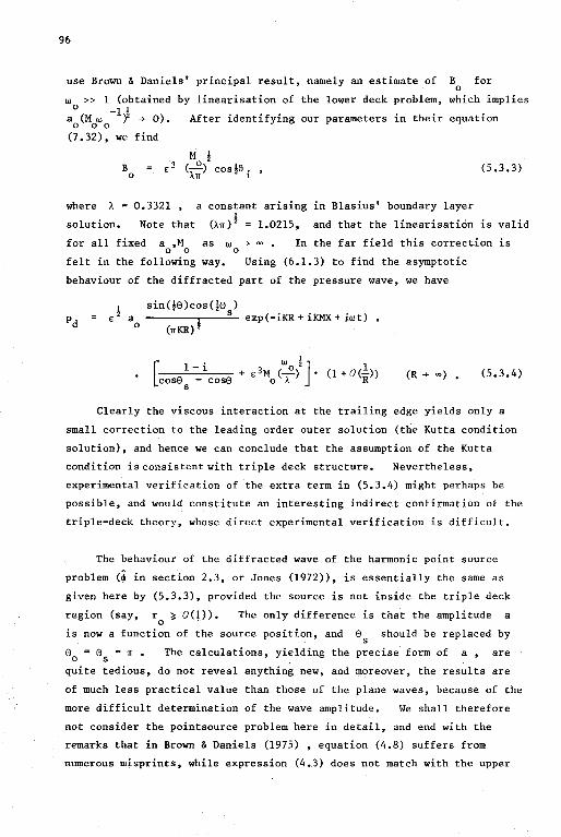
96

use Brown & Daniels' principal result, namely an estimate of B 0

for

w >> 1 (obtained o -11

by linearisation of the lower deck problem, which implies

a (Mw f ->- 0). 0 0 0

After identifying our parameters in their equation

(7. 32), we find

B 0

where À = o.3321

(5.3.3)

a constant arising in Blasius' boundary layer !

solution. Note that (Àrr) 2 = 1.0215, and that the linearisatión is valid

for all fixed a ,M as w ->- oo • In the far field this correction is 0 0 0

felt in the following way. Using (6.1.3) to find the asymptotic

behaviour of the diffracted part of the pressure wave, we have

! sin(j0)cos00s) e: a ----~--;:;__ exp(-iKR + iKMX + iwt) •

0 (rrKR) ~

[- 1 . w !] 1

- i + e:3M (....E.) • (1 +0(-)) cos0 - cose o À R

s (R ->- oo) • (5.3.4)

Clearly the viscous interaction at the trailing edge yields only a

small correction to the leading order outer solution (the Kutta condition

solution), and hence we can conclude that the assumption of the Kutta

condition is consistent with triple deck structure. Nevertheless,

experimental verification of the extra term in (5.3.4) might perhaps be

possible, and would constitute an interesting indirect confirmation of the

triple-deck theory, whose direct experimental verification is difficult.

The behaviour of the diffracted wave of the harmonie point source

problem (~ in section 2.3, or Jones (1972)), is essentially the same as

given here by (5.3.3), provided the source is not inside the triple deck

region (say, ro ~ o<i>>. The only difference is that the amplitude a

is now a function of the source position, and 0s should be replaced by

The calculations, yielding the precise form of a , are 0 = 0 - rr • 0 s

quite tedious, do not reveal anything new, and moreover, the results are

of much less practical value than those of the plane waves, because of the

more difficult determination of the wave amplitude. We shall therefore

not consider the pointsource problem here in detail, and end with the

remarks that in Brown & Daniels (1975) , equation (4.8) suffers from

numerous misprints, while expression (4.3) does not match with the upper

97

deck expression (5.9). In (5.9) an 3/2 O(E ) term is missing, but it

appears to be onl.y a constant which does not imply any further change.

5.4 Harmonie plane waves with a mixing Zayer

As was explained in the introduction 5.1, the main lines of reasoning

in the unsteady mixing layer problem are the same as those in the unsteady

wake problem. Here we shall use Daniels' (1978) incompressible viscous

solution as the inner solution to match our compressible inviscid solution

found in chapter 3. The relevant variable is the pressure on the flow

side, expressed by equations (3.4.21) and (3.4.23), or, approximated, by

(3.6.17) and (3.6.19). After application of (6.1.2), we find for the

normalized pressure in the triple deck region near the plate (y = -0,

x < 0)

constants +

where

k j [ 8

1 J E2 a 2(l+i) (-) ~ + --0 'IT 3 ~

and B 0

3

exp(iwt) + ••• , (5,4.1)

Daniels (1978) linearizes the fundamental lower-deck problem in the limit

of small amplitude, and finds an estimate of B1

for w >> 1 (in our 0

terminology). Ris expression (4.9)

p 0, -9,

where h is the amplitude,

+ ••• } '

S the Strouhal number, the constant

À = 0.3321 and his x2

is our x3 , is essentially the same as our

equation (5.4.1), provided we take the complex conjugates,as Daniels' time

dependence is exp(-iwt). Identification of the different terms yields

98

s IJ) +""

) 0

exp (-i2.11) M h* 0 8

+ 0 ' a 25/4 0 IJ)

0

lrl B E [M0 (w0À)

2

0

Note that the condition h+O is automatically satisf ied when

with the other parameters fixed,

The most interesting far field is in the still region, with

(5,4.2)

(5.4.3)

IJ) +"" 0

1T e < 1T • 4 < Taking into account the above viscous correction we have

there (cf. (3.6.20); use (3.6,16) and (6.1.3))

! ! E 2 a .!_ (~)

0 4 1T

2w0 ! ] - E3M (~-) sinje exp(iwt) + ,,,

0 À -(kr + 00) (5.4.4)

We see that the contribution of the viscous correction is even smaller

than the sound associated with the vortex shedding, while both are smaller

than the error terms inherent in equation (3.6.14), the approximated

version of (3.4,18), Obviously a better approximation of (3.4.18) is

needed, which is not readily to hand, however, Therefore we have to

conclude that as yet the use of expression (5,4.4) is limited to showing

when and how deviations occur from the full Kutta condition state, and of

what kind these deviations are.

We finally note that Hautus & Brands (1976) have proved the

existence and uniqueness of the most important function in the problem of

the mixing layer near the edge (Daniels (1977)), It is the function f0

,

def ined by f " ' + ~ f f " - l f ' 2 o f ' "' À n + o as n + "" , o 300 3o o

f0

' + 0 as n + - "" (equations (2.9) and (4.11) in Daniels (1977)), The

non-linear character of the equation made it far from obvious whether the

boundary conditions were possible,compatible, superfluous or sufficient,

It turned out that they were possible, compatible, and just sufficient.

5.5 Conolusions

We have discussed the mechanism of the viscous smoothing process at

the trailing edge in our acoustic problems of chapters 2 and 3, resulting

in the application of the Kutta condition to the inviscid outer solution.

Making use of the work of Brown & Daniels (1975) and Daniels (1978), we

derived an outer field correction, due to viscous action at the edge, for

high Reynolds numbers. It appears that an incident pressure wave with a

dimensionless amplitude of order /€ andfrequency of order E-z almost

satisfies the Kutta condition;

with an amplitude of order E 3 a multiple of the singular eigensolution

is to be added. It is conjectured that

when a pressure wave, satisfying the Kutta condition, behaves near the

edge like p = const. + A(w,M)/r exp(iwt), where A = O(IË), the

Kutta condition will, indeed, have a rational basis.

99

100

chapter 6

APPENDICES

6.1 Proper>ties of Fr>esneZ's integr>aZ F

definition

F(z) exp(iz2) f exp(-it2) dt

z

series expansion

(6.1.1)

F(z) Îl7i exp(-iÎ)(l + i z2 -Ïz" -ii z6 + ".)

- z ( 1 + ~ i' z2 - ..!_ z" 8 · 6 ) 3 15 - 105 l z + •••

l (i z2)n {....!.. .!. l7i exp(- i.'!!.) n=O n! 2 4

asymptotic behaviour

- 22n n! z}

(2n+l) !

(z -+ 0) = (6.1.2)

(-co< z <co),

F(z) i 1 1 - - + - + 0(-)

2z 4z3 z5 , 1 z 1 -+ co in -TI < arg z < I ,

i 1 1 l7i exp(-i-'+47T iz2) - - + - + 0(-), lzl-+ co in f~arg z ~ 1T.

2z 4z3 z5

(6.1.3)

functional relations

F(z) + F(-z) /7i exp(-iÎ + i z2), (6.1.4)

d dz F(z) 2 i z F(z) - 1 , (6.1.5)

101

exp(- i z2) r exp(i t 2) dt i F(-iz) (6.1.6) J z

We note that the function F has been tabulated for complex z by

Clemmow & Munford (1952) and Rankin (1949).

In flat plate diffraction problems, F is aften met with the argument

(2kr)! sinj(e ± e ). Therefore it is useful to complete this section 0

with notes on this argument in particular.

De fine y (2kr)! sin! (e - e ) 0

y (2kr)! sin! (e + e ) 0

then we have (index x{y) denotes differentiation w.r.t. x(y))

1 1 -

- 2r y (~)' 1 ( ) 2r sin 2 e + e 0

k l <2r) cos l (e + e

0)

l k (case - case 0

)

l k (sine - sine 0

)

2k l . - <-;-> sm l e cos l e 0

2k l 1 <-;-> cos 2 e cos l e 0

(2k) l cos l e · f ~ exp (-ikr + ikx case )dx = o r2 o

(6.1.7)

(6.1. 8)

(6.1.9)

(6.1.10)

(6.1.11)

(6.1.12)

(6.1.13)

{F(y) + F{y)} exp (-ikr + ikx cos6 ) + { function of y }. 0

102

6.2 Properties of Lerah's transaendent ~

Re sul ts are given for ~ in the form in which we meet i.t in

chapter4, i.e. exp(vy) ~(-expy,2,v).

Directly from the def inition, we have (for - ® < y ' O )

exp(vy) ® (-l)n exp(ny) }:---

(n + v) 2 ~ ( -exp y , 2 , v) exp(vy)

n=O (6.2.1)

Applying Gradshteyn & Ryzhik (9.554), (9.531), (9.623.3) and (8.363.8)

yields

exp(vy) ~ (- exp y , 2, v)

for IYI < 11 , where

_ .P'(v+l)} + 2

1 (2y)n - B (~)} ~~_.,_,,__,~

n+l 2 (n+l) (n+2) ! (6.2.2)

Bn(x) is the n-th order Bernoulli polynomial according to the definition

of Gradshteyn & Ryzhik (9.62), and

iji(x) is the logarithmic derivative of Euler's gamma function (Gradshteyn

& Ryzhik (8.360)).

Some numerical values (Abramowitz & Stegun (1965)) are

ijl' (l) 8

- ijl' (2) 8

6.1560

ijl(l) 8

- ijl (2) 8

- /2 11 + /2 log (3 + 2 12) -1. 9500

ijl' (l) 8

- ijl' (2..) 8

64 - 4 .fi 11 2 - ijl' (l) 8

+ijl' <i) 2.0130

ijl(l) 8

- ijl (2..) 8

12 11 + /2 log (3 + 2 12) - 8 -1. 0642

3 - B (2) l 5 9 Bl (3) 1 8 - 2 Bl (3) Bl (3) -2

3 7 1 5 9 3 B2 (3) B2 (3) - 8 B2 (3) B2(8) 8

3 7 9 5 - B (2_) 15 B3 (3) B3 (3) ill B3 (3) . 3 8 - ill

3 - B (!_.) 11 5 - B (2_) 9 B4 (3) 4 8 256 B4 (3) 4 8 256

3 - B (!_.) 285 5 - B (2_) 275 BS (3) 5 8 - 8192 B5(3) 5 8 8192

For ,all y with - 00 < y < 0 , we find from Gradshteyn & Ryzhik (9.556)

that

103

exp ( vy) 1> ( - exp y , 2, v) 1 exp(vy)

1 - J ---...,-( y - - log t ) dt , (6.2.3) v 0 ! v

1 + tv

of which, for v=l±l , the term 1 exp(vy)

1 - f -- dt v 0 1

1 + tv

exp(!y) 3±1 4 J _x __ dx

0 1 + x4

can be expressed in elementary functions (Gradshteyn & Ryzhik (2.132)),

104

REFERENCES

Abramowitz, M. & Stegun, I.A. (ed.) (1965)

Handbook of Mathematical Functions, Dover Publ. , New York.

Acton, E. (1976)

The modelling of large eddies in a two-dimensional shear layer,

J, Fl. Mech,, J..2., 561-593.

Archibald, F.S. (1975)

Unsteady Kutta condition at high values of the reduced frequency

parameter, J, Aircraft, Jl, 545-550.

Batchelor, G.K. (1967)

An Introduction to Fluid Dynamics, Cambridge University Press.

Bechert, D. & Michel, U. (1975)

The control of a thin free shear layer with and without a semi­

infinite plate by a pulsating flow field, Acustica, ]1, 287-307.

Bechert, D., Michel, U. & Pfizenmaier, E. (1977)

Experiments on the transmission of sound through jets, AIAA-paper

no. 77-1278,

Bechert, D. & Pfizenmaier, E. (1975)

Optical compensation measurements on the unsteady exit condition at a

nozzle discharge edge, J, Fl. Mech., 2J., 123-144.

Boersma, J. (1978)

Private communication.

Browti, S.N. & Daniels, P.G. (1975)

On the viscous flow about the trailing edge of a rapidly oscillating

plate, J, Fl. Mech., ~. 743-761.

Brown, S.N. & Stewartson, K. (1970)

Trailing-edge stall, J. Fl. Mech., 42, 561-584.

Candel, S.M. (1973)

Diffraction of a plane wave by a half plane in a subsonic and

supersonic medium, J, Acoust. Soc. Am., 54, 1008-1016.

Candel, S.M. (1975)

Acoustic conservation prindples and an application to plane and

modal propagation in nozzles and diffusers, J, Sound and Vibr., i.!_,

207-232.

Clemmow, P.C. & Munford, C. (1952)

Phil. Trans. fil !• 189.

Crighton, D.G. (1972a)

Radiation properties of the semi-infinite vortex sheet, Proc. R. Soc.

Lond. ~ 1lQ_, 185-198.

Crighton, D.G. (1972b)

The excess noise field of subsonic jets, J, Fl. Mech., 56, 683-694.

Crighton, D.G. (1972c)

105

Radiation from vortex filament motion near a half plane, J, Fl. Mech.,

1.!_, 357-362.

Crighton, D.G. (1975)

Basic principles of aerodynamic noise generation, Prog. Aerospace

Science, ~. 31-96.

Crighton, D.G. & Leppington, F.G. (1974)

Radiation properties of the semi-infinite vortex sheet: the initial

value problem, J, Fl. Mech., 64, 393-414.

Crow, S.C. & Champagne, F.H. (1971)

Orderly structure in jet turbulence, J, Fl. Mech., 48, 547-591.

Curle, N. (1955)

The influence of solid boundaries upon aerodynamic sound, Proc. Roy.

Soc. ~. ~. 505-514.

Daniels, P.G. (1974)

Numerical and asymptotic solutions for the supersonic flow near the

trailing edge of a flat plate at incidence, J, Fl. Mech., 63, 641-656.

Daniels, P.G. (1977)

Viscous mixing at a trailing edge, Q. Jl. Mech. Appl. Math., 30,

319-342.

Daniels, P.G. (1978)

On the unsteady Kutta condition, Q. Jl. Mech. Appl. Math., 31. 49-75.

Davis, S.S. (1975)

Theory of discrete vortex noise, AIAA Journal, _!l, 375-380.

Dennis, S.C.R. & Dunwoody, J. (1966)

The steady flow of a viscous fluid pasta flat plate, J, Fl. Mech. 24,

577-595.

Ffowcs Williams, J.E. (1963)

The noise from turbulence convected at high speed, Phil. Trans. ~.

255, 469-503.

Ffowcs Williams, J.E. & Hall, L.H. (1970)

Aerodynamic sound generation by turbulent flow in the vicinity of a

scattering half plane, J. Fl. Mech., 40, 657-670.

106

Ffowcs Williams, J.E. & Hawkings, D.L. (1969)

Phil. Trans. !• !2i• 321-342.

Ffowcs Williams, J.E. & Kempton, A.J. (1978)

The noise from the large-scale structure of a jet, J, Fl. Mech., .!!!.• 673-694.

Friedland, A.B. & Pierce, A.D. (1969)

Reflection of acoustic pulses from stable and instable interfaces

between moving fluids, Phys. Fluids, _!l, 1148-1159.

Friedlander, F.G. (1958)

Sound Pulsès, Cambridge University Press.

Goldstein, M.E. (1976)

Aeroacoustics, McGraw-Hill, New York.

Goldstein, s. (1930)

Concerning some solutions of the boundary layer equations in

" hydrodynamica, Proc.Cambr. Phil. Soc., 26, 1-30.

Gottlieb, P. (1960)

Sound source near a velocity discontinuity, J. Acoust. Soc. Am., 32,

1117-1122.

Gradshteyn, I.S. & Ryzhik, I.M. (1965)

Table of Integrals, Series, and Products, Academie Press, New York.

Hautus, M.L.J. & Brands, J.J.A.M. (1976)

Private communication.

Heavens, S.N. (1978)

An experimental study of sound diffraction at an airfoil trailing

edge, J, Fl. Mech., 84, 331-335.

Heavens, S.N. (1979)

Acoustic excitation of a subsonic jet, preprint University of

Cambridge, England.

Hinze, J.O. (1975)

Turbulence, McGraw-Hill, New York, 2nd. ed ••

Howe, M,S. (1970)

Transmission of an acoustic pulse through a plane vortex sheet,

J. Fl. Mech., ~' 353-367.

Howe, M.S. (1976)

The influence of vortex shedding on the generation of sound by

convected turbulence, J. Fl. Mech., ~. 711-740.

Howe, M.S. (1978)

Attenuation of sound in a low Mach number nozzle flow, Bolt, Beranek

& Newman Ine. Report no. 3762; also:J. Fl, Mech., 2.!_, 209-229, 1979.

Jobe, C.E. & Burggraf, O.R. (1974)

The numerical solution of the asymptotic equations of trailing edge

flow, Proc. R. Soc.~. 340, 91-111.

Jones, D.S. (1964)

The Theory of Electromagnetism, Pergamon, London.

Jones, D. S, (1972)

Aerodynamic sound due to a source near a half-plane, J, Inst. Maths

Applics, 2_, 114-122.

Jones, D.S. & Morgan, J.D. (1972)

107

The instability of a vortex sheet on a subsonic stream under acoustic

radiation, Proc. Camb. Phil. Soc., 7l:_, 465-488.

Jones, D.S. & Morgan, J.D. (1974)

A linear model of a finite amplitude Helmholtz instability, Proc. R.

Soc. Lond. ~. 338, 17-41,

Landau, L. (1944)

Compt. Rend, Acad. Sci, USSR, 44, 139.

Lawrence, L.F., Schmidt, S.F. & Looschen, F.W. (1951)

A self-synchronizing stroboscopic schlieren system for the study of

unsteady air flows, NAGA, TN 2509.

Lee, B.H.K. & Jones, D.J. (1973)

Transmission of upstream sound through a subsonic jet, AIAA-paper

no. 73-630.

Lighthill, M.J. (1952)

On sound generated aerodynamically, I. General theory, Proc. R. Soc.

~. ~. 564-587,

Lighthill, M.J. (1954)

On sound generated aerodynamically, II. Turbulence as a source of

sound, Proc. R. Soc. ~. ~. 1-32.

Messiter, A.F. (1970)

Boundary-layer flow near the trailing edge of a flat plate, SIAM J,

Appl. Math., ~. 241-257.

Miles, J.W. (1957)

On the reflection of sound at an interface of relative motion,

J. Acoust. Soc. Am., ~. 226-228.

108

Moore, C.J. (1977)

The role of shear-layer instability waves in jet exhaust noise,

J, Fl. Mech., ~· 321-367.

Morgan, J.D. (1974)

The interaction of sound with a semi-infinite vortex sheet, Q. Jl.

Mech. Appl. Math., JJ_, 465-487.

Morgan, J.D. (1975)

The interaction of sound with a subsonic cylindrical vortex layer,

Proc. R. Soc. Lond. !:_, 344, 341-362.

Munt, R.M. (1977)

The interaction of sound with a subsonic jet issuing from a semi­

infinite cylindrical pipe, J. Fl. Mech., 83, 609-640.

Noble, B. (1958)

Methods based on the Wiener-Hopf Technique, Pergamon, London.

Orszag, S.A. & Crow, S.C. (1970)

Instability of a vortex sheet leaving a semi-infinite plate,

Stud. Appl. Math" 49, 167-181.

Pinker, R.A. & Bryce, W.D. (1976)

The radiation of plane wave duet noise from a jet exhaust, statically

and in flight, A.I.A.A. paper no, 76-581

Poldervaart, L.J., Wijnands, A.P.J., van Moll, I.H.A.M. & van Voorthuisen,

E.J. (1974)

"Modes of Vibration", (film).

Poldervaart, L.J., Wijnands, A.P.J. & Bronkhorst, I. (1974)

"Sound Pulse-Boundary Layer Interaction Studies", (film), A.V. Cent re,

T.H.E., Eindhoven, Netherlands. Reviewed by J.E. Ffowcs Williams,

J. Fl. Mech., 78, 859-862, (1976).

Rankin, R.A. (1949)

Phil. Trans., 3i!_ !:_, 457.

Ribner, H.S. (1957)

Reflection, transmission, and amplification of sound by a moving

medium, J. Acoust. Soc. Am., 29, 435-441.

Riley, N. & Stewartson, K. (1969)

Trailing edge flows, J. Fl. Mech., 39, 193-207.

Rosenhead, L. (ed.) (1963)

Laminar Boundary Layers, Oxford University Press.

Smith, F.T. (1977)

The laminar separation of an incompressible fluid streaming past a

smooth surface, Proc. R. Soc. Lond. !:_, 356, 443-463.

Stewartson, K. (1969)

On the flow near the trailing edge of a flat plate II, Mathematika,

_!2., 106-121.

Stewartson, K. & Williams, P.G. (1969)

Self-induced separation, Proc. R. Soc. Land., ~. 111.• 181-206.

Van Dyke, M. (1975)

Perturbation Methods in Fluid Mechanics, Parabolic Press, Stanford,

annotated edition.

Veldman, A.E.P. (1976)

Boundary layer flow past a finite flat plate, Ph.D. thesis,

Rijksuniversiteit Groningen.

Watson, G.N. (1966)

A Treatise on the Theory of Bessel Functions, Cambridge University

Press, 2nd ed •.

109

110

LEVENSLOOP

10 maart 1952

1964 - 1970

1970 - juni 1975

augustus 1975 - juni 1979

NAWOORD

- geboren te Manado, Indonesië

- gymnasium B, Openbare Scholengemeenschap,

Utrecht

doctoraalstudie Wiskunde, Rijksuniversiteit

Utrecht; afstudeerrichting "toegepaste

analyse" bij prof.dr.ir. W. Eckhaus

wetenschappelijk medewerker aan de T.H.E.,

vakgroep Transportfysica

Allen die mij hebben geholpen bij de totstandkoming van dit

proefschrift wil ik hierbij hartelijk danken. In het bijzonder noem ik:

de leden van de vakgroep, speciaal de mede L.T.D.-ers, voor de

prettige samenwerking en de vriendschappelijke sfeer; bovendien nog apart

ir. L,J, Poldervaart die mij aanzette tot het leggen van de contacten

met Engeland,

de Universiteit van Leeds voor de gastvrijheid, en de medewerkers

van het Applied Mathematica Department aldaar voor de enthousiaste

ontvangst en belangstelling,

mrs P. Jowett en mevrouw H. Weisè voor het vlot en keurig

verzorgde typewerk, en Ruth Gruyters voor de nette tekeningen.

lil

SAMENVATTING

Dit proefschrift behandelt de interactie van geluid met een stroming. Er

worden drie modellen bestudeerd waarin steeds de aanwezigheid van een

afstroomrand een centraal element vormt. Een uniforme subsone wrijvingsloze

compressibele stroming aan één of beide zijden van een half oneindige dunne

vlakke plaat, en in een half oneindige dunwandige open pijp wordt verstoord

door geluid,

én het probleem met een stroming aan beide zijden van de plaat worden een

Jlindrische geluidspulsen een vlakke harmonische geluidsgolf verstrooid

door de rand en de stroming. Expliciete resultaten, exact binnen de

gebruike, '.jke linearisering, zijn verkregen voor het resulterende veld.

Afhankelijk van de mate van het bij de rand op te leggen singulier gedrag

van de oplossing, wordt aan de rand wervelsterkte geproduceerd. Deze wervels

maken zich akoestisch kenbaar in de diffractie golf. De reguliere oplossing,

met maximale wervelproduktie (de Kutta voorwaarde is dan geldig), heeft

stroomopwaarts een lagere en stroomafwaarts een hogere drukamplitude dan de

singuliere oplossing zonder wervelproduktie.

In het probleem met een stroming aan één zijde wordt een vlakke harmonische

geluidsgolf, komend van stroomopwaarts vanuit de stroming, weer verstrooid

aan de rand en genereert, afhankelijk van de op te leggen randsingulariteit,

wervelsterkte. We hebben nu echter achter de plaat een tangentiële

cnelheids-discontinuiteit (wervellaag) in de hoofdstroom. De hierin

inL. ·ente Helmholtz instabiliteit wordt aangeslagen indien wervels worden

gegenereerd, waardoor het hydrodynamische veld ingrijpend kan worden

gewijzigd. Exacte oplossingen in integraalvorm worden gepresenteerd,

waarbij wordt aangetoond dat het de conditie aan de plaatrand is die de

instabiliteit beheerst, en niet een zekere causaliteits eis, ingevoerd door

vroegere auteurs. Uit de exacte oplossingen worden expliciete benaderingen

verkregen, geldig voor kleine waarden van het Mach getal.

In het pijpprobleem komen vlakke harmonische geluidsgolven van stroom­

opwaarts uit de pijp. Naast diffractie en de produktie van wervelsterkte

treedt nu ook reflectie aan het open pijp uiteinde op. Exacte oplossingen,

weer in integraalvorm, worden benaderd in de limiet van lange golven (klein

Strouhal getal) door expliciete uitdrukkingen. Onhafhankelijk van de

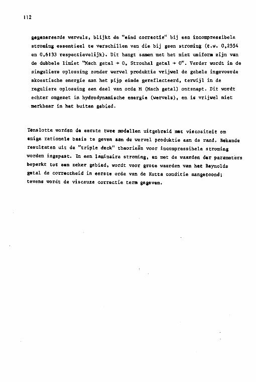
112

gegenereerde wervels, blijkt de "eind correctie" bij een incompressibele

stroming essentieel te verschillen van die bij geen stroming (t.w. 0,2554

en 0,6133 respectievelijk). Dit hangt samen met het niet uniform zijn van

de dubbele limiet "Mach getal-+ 0, Strouhal getal-+ O". Verder wordt in de

singuliere oplossing zonder wervel produktie vrijwel de gehele ingevoerde

akoestische energie aan het pijp einde gereflecteerd, terwijl in de

reguliere oplossing een deel van orde M (Mach getal) ontsnapt. Dit wordt

echter omgezet in hydrodynamische energie (wervels), en is vrijwel niet

merkbaar in het buiten gebied.

Tenslotte worden de eerste twee modellen uitgebreid met viscositeit om

enige rationele basis te geven aan de wervel produktie aan de rand. Bekende

resultaten uit de "triple deck" theorieën voor incompressibele stroming

worden ingepast. In een laminaire stroming, en met de waarden der parameters

beperkt tot een zeker gebied, wordt voor grote waarden van het Reynolds

getal de correctheid in eerste orde van de Kutta conditie aangetoond;

tevens wordt de visceuze correctie term gegeven.

-4

Addendum to chapter 4.

The waves, diffracted at the pipe exit, are given in

(4.4. 16,17,22,23) in terms of the functions Z0(r,z') and

(see (4.4. 18, 19)). These are approximated on the pipe axis

Z 1 (r,z')

r = 0 by

(4.4.28,29). After numerical integration of the respective expressions

(6.2.3), these approximations of zo,I (O,z') are (on logarithmic scale)

given by the following diagrams:

-3 -2 -1 0 2 3

z '-axis

-7

4

STELLINGEN

1. Beschouw het "forward-time centred-space" differentie schema voor de

numerieke oplossing van de tweedimensionale tijdsafhankelijke Navier­

Stokes vergelijkingen.

De opvatting, zoals bv. geponeerd door Roache, dat de zg. "cell­

Reynolds number" conditie voldoende en noodzakelijk is voor stabiliteit

van het schema, volgt niet uit berekeningen. Voor ingewikkelde

configuraties is het de vraag of de conditie is te bewijzen, en voor

eenvoudige is de conditie te verscherpen. Bijvoorbeeld wanneer de

stromingssnelheidsvector in het rekenpunt langs een der assen van het

rooster is gericht (zegge (u0 ,0)), is

uÖM < v '

2

(lokaal) voldoende en noodzakelijk voor (lineaire) stabiliteit.

Roache, P.J., Computational Fluid Dynamics, 1976, Hermosa, Albuquerque,

p. 42-45.

2. Gradshteyn & Ryzhik's eigen definitie van Bernoulli polynomen (9.62)

laten een vereenvoudiging toe van Gradshteyn & Ryzhik (9.531).

Gradshteyn & Ryzhik, Table of Integrals, Series and Products, 1965,

Acad. Press, New York.

3. De oplossing van het probleem van de "lange zware kabel" wordt door

Plunkett gegeven in de vorm van een asymptotische reeks naar een kleine

parameter a. Slechts de eerste term van deze reeks is correct. Dit

vindt zijn oorzaak in het feit dat hij een voorkomende functie B(z,a)

ontwikkelt naar machten van a 2 in plaats van a. Dit kan de door Pedersen

aan Plunkett's oplossing toegeschreven beperkingen verklaren.

Plunkett, R., Trans ASME, J. Engin. Indus., 89, 31-36, 1967.

Pedersen, P.T., Intern. Shipbuilding Prog., ~. 399-408, 1975.

4. Beschouw de differentiaalvergelijking x = f(y') voor y = y(x) op [0,00).

Zij y0 tussen de reële getallen a en S, - 00 ~ a,S ~ 00 , met y(O) = y0 ,

f(a) = 0, f(S) = oo. Tussen a en S is f monotoon, positief en continu.

Noem f(s) = F'(s).

Indien de vergelijking asymptotisch is te inverteren tot

À -1 À -1 "-1-1 y' (x) a À x n + • . . + a À x 0

, + bx-1 + a..1 À-1 x +

dan

y(x)

n n o o

À -1 + a À x -m+l

À -1 -m

+ O(x -m+l -m+1

is À À

= n + 0 + b log a x ... + a x n 0

À À -1 -m+1 a x + ... + a -m+lx -1

(x-+- oo),

x + A +

À + O(x -m)

À

waarbij A = y + [t f(t) - F(t) - a f n(t) -o n

- b log(I + f(t))] 13 • Cl

(x+oo),

À -af 0

(t) 0

5. De procedure van het bloksgewijs matchen, die Crighton & Leppington

voorstellen, wanneer in de termen van een asymptotische reeks naar een

kleine parameter E zowel machten van E als van log E als factor voor­

komen, laat zich omschrijven als: beschouw log E van orde 1. Dit is

inderdaad vaak het geval in fysische toepassingen.

Crighton, D.G. & Leppington, F.G., Proc. R. Soc. Lond. !:_, ~. 313-339,

1973.

6. Aangezien de door Shivamoggi voorgestelde vereenvoudigde matchings­

procedure slechts in een beperkt aantal gevallen toepasbaar is, en dan

ofwel te zeer voor de hand ligt om een apart formalisme aan te wijden,

ofwel pas achteraf toepasbaar blijkt, levert deze procedure geen enkel

voordeel op boven de bestaande algemenere methoden.

Shivamoggi, B.K., ZAMM., 58,354-356, 1978.

7. De interpretatie door Ffowcs Williams van Howe's werk is niet correct.

Ffowcs Williams, J.E., Aeroacoustics, Ann. Rev. Fl. Mech. 1977,

p. 454, 455.

8. Beschouw het probleem van lange geluidsgolven in een halfoneindige open

pijp, waaruit lucht stroomt met Mach getal M, 0 ~ M < 1. De parameter,

representerend de faseverschuiving van de golf na reflectie tegen het

open pijpuiteinde, wordt genoemd de "eind correctie". Dimensieloos is

deze, bij afwezigheid van stroming, gelijk aan: 0,6133, en bij een

incompressibele stroming: 0,2554. In beide gevallen is M = O.

Dit proefschrift.

9. Lezen is het herkennen van woordbeelden en niet het aaneenrijgen van

letters. Wijzigingen in de spelling moeten dan ook slechts na zeer

zorgvuldige overwegingen ingevoerd worden.

JO. Indien het voor iemand openhouden van een zich zelf sluitende deur

bedoeld is als beleefd gebaar, dient nauwkeurig in acht te worden

genomen de snelheid en de afstand tot de deur van degene, tot wie dit

gebaar is gericht. Indien hij gedwongen wordt zijn pas te versnellen,

om niet zelf onbeleefd te lijken, is het gebaar niet zo beleefd meer.

Sjoerd W. Rienstra

Eindhoven, 8 juni 1979