Edge Detection from Spectral Data With Applications to PSF … · Edge Detection from Spectral Data...

Edge Detection from Spectral DataWith Applications to PSF Estimation and Fourier Reconstruction

Aditya Viswanathan

School of Electrical, Computer and Energy Engineering, Arizona State [email protected]

Oct 22 2009

Aditya Viswanathan (Arizona State University) Edge Detection from Spectral Data Oct 22 2009 1 / 41

Prof. Anne Gelb is with the School of

Mathematical and Statistical Sciences,

Arizona State University

Prof. Douglas Cochran is with the School of

Electrical, Computer and Energy

Engineering, Arizona State University

Prof. Rosemary Renaut is with the School of

Mathematical and Statistical Sciences,

Arizona State University

Dr. Wolfgang Stefan is with the Department

of Computational and Applied Mathematics,

Rice University

Research supported in part by National Science Foundation grants

DMS 0510813 and DMS 0652833 (FRG).


Introduction Motivation

Why do we need edge data?

Solve PDE’s with shocks moreaccurately.

Identify tissue boundaries inmedical images and segment them.

Reconstruct piecewise-analyticfunctions from Fourier and otherspectral expansion coefficients withuniform and exponentialconvergence properties.

0 0.2 0.4 0.6 0.8 1 1.2 1.4 1.6 1.8 2−4

−2

0

2

4

x (x pi)

Un(

x,t)

PDE Solution

0 0.2 0.4 0.6 0.8 1 1.2 1.4 1.6 1.8 2−10

−5

0

5Jump Function Approximation

[f](x

)

x

True Solutiontf = 0

tf = 50, Exp. Filtering, p=2


tf = 0



(a) PDE solution withshock discontinuity

(b) MRI tissue bound-ary detection

−3 −2 −1 0 1 2 3−2.5

−2

−1.5

−1

−0.5

0

0.5

1

1.5

2

2.5Function Reconstruction

x

g(x

)

TrueFourier reconstruction

(c) Fourier reconstruc-tion showing Gibbs

−3 −2 −1 0 1 2 3−2.5

−2

−1.5

−1

−0.5

0

0.5

1

1.5

2

2.5Function Reconstruction

x

g(x

)

TrueAlt. reconstruction

(d) Alt. reconstruction


Introduction Motivation

Application – Magnetic Resonance Imaging

020

4060

80100

120

0

50

100

0

0.2

0.4

0.6

0.8

1

ωkx

Fourier Coefficients

ωky

|f(ω

kx,ω

ky)|

(e) Acquired Fourier Samples

−0.5 −0.4 −0.3 −0.2 −0.1 0 0.1 0.2 0.3 0.4 0.5−0.5

−0.4

−0.3

−0.2

−0.1

0

0.1

0.2

0.3

0.4

0.5

kx

k y

Spiral scan trajectory

(f) Sampling Trajectory

Reconstructed phantom

(g) Reconstructed Image

Figure: MR Imaginga

aSampling pattern courtesy Dr. Jim Pipe, Barrow Neurological Institute,Phoenix, Arizona


Introduction Problem Statement

Problem Statement

Objective: To recover location, magnitude and sign of jump discontinuities from a finitenumber of spectral coefficients

Assumptions:

f is 2π-periodic and piecewise-smooth function in [−π, π).

Its jump function is defined as

[f ](x) := f(x+)− f(x−)

It has Fourier series coefficients

f(k) =1

2π

Z π

−πf(x)e−ikxdx , k ∈ [−N,N ]

A jump discontinuity is a local feature; i.e., the jump function at any point x onlydepends on the values of f at x+ and x−. However, f is a global representation; i.e.,f(k) are obtained using values of f over the entire domain [−π, π).


Concentration Method

Outline

1 IntroductionMotivationProblem Statement

2 Jump detection using the Concentration methodThe Concentration MethodConcentration FactorsStatistical Analysis of the Concentration MethodIterative Formulations

3 ApplicationsPSF Estimation in Blurring ProblemsApplications to Fourier Reconstruction


Concentration Method The Concentration Method

Getting Jump Data from Fourier Coefficients

Let f contain a single jump at x = ζ.

f(k) =1

2π

Z π

−πf(x)e−ikxdx

=1

2π

Z ζ−

−πf(x)e−ikxdx+

Z π

ζ+f(x)e−ikxdx

!

=1

2π

f(x)

e−ikx

−ik

˛ζ−−π−Z ζ−

−πf ′(x)

e−ikx

−ik dx

+ f(x)e−ikx

−ik

˛πζ+−Z π

ζ+f ′(x)

e−ikx

−ik dx

«

=1

2π

f(ζ−)e−ikζ − f(−π)eikπ

−ik −Z ζ−

−πf ′(x)

e−ikx

−ik dx

+f(π)e−ikπ − f(ζ+)e−ikζ

−ik −Z π

ζ+f ′(x)

e−ikx

−ik dx

«



Getting Jump Data from Fourier Coefficients

f(k) =1

2π

f(ζ−)e−ikζ − f(−π)eikπ

−ik −Z ζ−

−πf ′(x)

e−ikx

−ik dx

+f(π)e−ikπ − f(ζ+)e−ikζ

−ik −Z π

ζ+f ′(x)

e−ikx

−ik dx

«

=`f(ζ+)− f(ζ−)

´ e−ikζ2πik

+f(−π)eikπ − f(π)e−ikπ

2πik+O

„1

k2

«Since f is periodic, f(−π) = f(π) and the second term vanishes.

f(k) = [f ](ζ)e−ikζ

2πik+O

„1

k2

«



Extracting Jump Information

Let us compute a ‘filtered’ partial Fourier sum of the form

SN [f ](x) =

NXk=−N

„iπk

N

«f(k)eikx

SN [f ](x) =NX

k=−N

„iπk

N

«f(k)eikx

=NX

k=−N

„iπk

N

«»[f ](ζ)

e−ikζ

2πik+O

„1

k2

«–eikx

= [f ](ζ)1

2N

NXk=−N

eik(x−ζ) +

NXk=−N

O„

1

k

«eik(x−ζ)

First term is a scaled (by the jump value) Dirac delta localized at x = ζ (the jumplocation)

The second term is a manifestation of the global nature of Fourier data



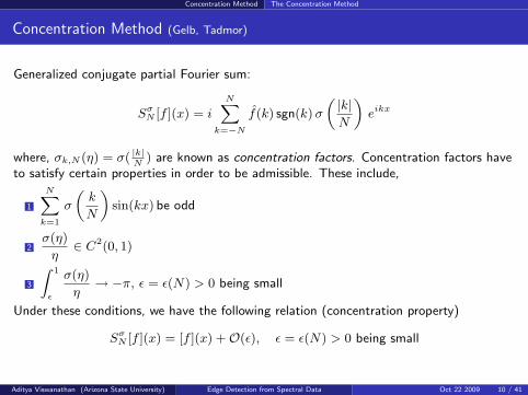
Concentration Method (Gelb, Tadmor)

Generalized conjugate partial Fourier sum:

SσN [f ](x) = i

NXk=−N

f(k) sgn(k)σ

„|k|N

«eikx

where, σk,N (η) = σ( |k|N

) are known as concentration factors. Concentration factors haveto satisfy certain properties in order to be admissible. These include,

1

NXk=1

σ

„k

N

«sin(kx) be odd

2σ(η)

η∈ C2(0, 1)

3

Z 1

ε

σ(η)

η→ −π, ε = ε(N) > 0 being small

Under these conditions, we have the following relation (concentration property)

SσN [f ](x) = [f ](x) +O(ε), ε = ε(N) > 0 being small



Illustration of the Concentration Method


Concentration Method Concentration Factors

Classical Concentration Factors

Factor Expression

Trigonometric σT (η) =π sin(αη)

Si(α)

Si(α) =

Z α

0

sin(x)

xdx

Polynomial σP (η) = −p π ηpp is the order of the factor

Exponential σE(η) = C η exp

„1

αη (η − 1)

«C - normalizing constant; α - order

C =πR 1− 1

N1N

exp“

1α τ (τ−1)

”dτ

Table: Examples of concentration factors



Concentration Factors - Visualization in Fourier Space

−80 −60 −40 −20 0 20 40 60 800

0.5

1

1.5

2

2.5

3

3.5

4

k

sig(

eta)

Concentration Factors

TrigonometricPolynomialExponential

Figure: Envelopes of the Concentration Factors in Fourier Space



Concentration Factors - Typical Responses

−3 −2 −1 0 1 2 3−3.5

−3

−2.5

−2

−1.5

−1

−0.5

0

0.5

1

1.5

2

SN

[f](x

)

x

fS

N[f]

(a) Trigonometric Factor

−3 −2 −1 0 1 2 3−3.5

−3

−2.5

−2

−1.5

−1

−0.5

0

0.5

1

1.5

2

SN

[f](x

)

x

fS

N[f]

(b) Polynomial Factor

−3 −2 −1 0 1 2 3−3.5

−3

−2.5

−2

−1.5

−1

−0.5

0

0.5

1

1.5

2

SN

[f](x

)

x

fS

N[f]

(c) Exponential Factor

Figure: Characteristic Responses of the Concentration Factors to a Sawtooth Function



Examples

−3 −2 −1 0 1 2 3−2

−1.5

−1

−0.5

0

0.5

1

1.5

2

x

f(x)

Jump Approximation − Trigonometric Factor

f

SN

[f]


−3 −2 −1 0 1 2 3

−1

−0.8

−0.6

−0.4

−0.2

0

0.2

0.4

0.6

0.8

1

x

f(x)

Jump Approximation − Exponential Factor

fS

N[f]

(b) Exponential Factor

Figure: Jump Response, N = 128

For images, we apply the concentrationmethod to each dimension separately

SσN [f ](x(y)) = iNX

l=−N

sgn(l)σ

„|l|N

«

·NX

k=−N

fk,l ei(kx+ly)

where the overbar represents thedimension held constant.



Examples

−3 −2 −1 0 1 2 3−2

−1.5

−1

−0.5

0

0.5

1

1.5

2

x

f(x)

Jump Approximation − Trigonometric Factor

f

SN

[f]


−3 −2 −1 0 1 2 3−1

−0.8

−0.6

−0.4

−0.2

0

0.2

0.4

0.6

0.8

1

x

f(x)

fS

N[f]

(b) Trigonometric Factor

Figure: Jump Response, N = 128

For images, we apply the concentrationmethod to each dimension separately

SσN [f ](x(y)) = iNX

l=−N

sgn(l)σ

„|l|N

«

·NX

k=−N

fk,l ei(kx+ly)

where the overbar represents thedimension held constant.



Concentration Factor Design (Viswanathan, Gelb)

Choose a template function f , eg. the sawtooth function

f(x) =

x−π

2x < 0

x+π2

x > 0[f ](x) =

−π x = 00 else

Design σ such that SσN [f ](x) = iNX

k=−N

f(k) sgn(k)σ

„|k|N

«eikx closely matches

[f ].

Typical problem formulation

minσ

φ0(σ)

subject to φm(σ) = cm,

ψn(σ) ≤ cn

where cm, cn are constants and the objective and constraints are typically normmeasures or the conjugate partial sum evaluated at certain points/intervals in thedomain.



Equivalence of Constraints and Admissibility Conditions

1

NXk=1

σ

„k

N

«sin(kx) be odd ⇐⇒ conjugate kernel real, odd; hence

σ(−η) = σ(η) with σ(0) = 0.

2σ(η)

η∈ C2(0, 1) ⇐⇒ include ‖σ‖2 or similar smoothness

metric in objective.

3

Z 1

ε

σ(η)

η→ −π, ε = ε(N) > 0 ⇐⇒ SσN [f ](ζ) = [f ](ζ)

ζ being a point of discontinuity.

(2) is not really an equivalence, but this turns out be practically inconsequential.



Examples

Problem Formulation 1

minσ

‖ [f ]− SσN [f ] ‖2

subject to SσN [f ](0) = −π


minσ

‖ [f ]− SσN [f ] ‖1

subject to SσN [f ](0) = −π


minσ

‖ [f ]− SσN [f ] ‖1

subject to SσN [f ](0) = −π|SσN [f ](x)| ≤ 10−3, |x| ∈ (0.25, 3)

−4 −3 −2 −1 0 1 2 3 4−4

−3

−2

−1

0

1

2

x

[f](x

)

fS

N[f]

(a) Response

−80 −60 −40 −20 0 20 40 60 800

0.5

1

1.5

2

2.5

3

3.5

k

σ(k)

(b) Conc. Factor

Figure: Problem Formulation 1, N = 64

−4 −3 −2 −1 0 1 2 3 4−4

−3

−2

−1

0

1

2

x

[f](x

)

fS

N[f]

(a) Response

−80 −60 −40 −20 0 20 40 60 800

0.5

1

1.5

2

2.5

3

k

σ(k)

(b) Conc. Factor

Figure: Problem Formulation 2, N = 64

−4 −3 −2 −1 0 1 2 3 4−4

−3

−2

−1

0

1

2

x

[f](x

)

fS

N[f]

(a) Response

−80 −60 −40 −20 0 20 40 60 800

0.5

1

1.5

2

2.5

3

3.5

k

σ(k)

(b) Conc. Factor

Figure: Problem Formulation 3, N = 64Aditya Viswanathan (Arizona State University) Edge Detection from Spectral Data Oct 22 2009 18 / 41


The Missing Coefficient Problem

Let us assume that mid-range Fourier coefficients are missing (eg., modes |30− 40|for N = 64).

Since the response and kernel are real, we assume that both f(±p) are missing.

Use of the standard concentration factors results in spurious oscillations in smoothregions.

−4 −3 −2 −1 0 1 2 3 4−3

−2.5

−2

−1.5

−1

−0.5

0

0.5

1

1.5

2

x

[f](x

)

fS

N[f]

(a) Response – Trigonometric factor

−4 −3 −2 −1 0 1 2 3 4−2.5

−2

−1.5

−1

−0.5

0

0.5

1

1.5

2

x

[f](x

)

fS

N[f]

(b) Response – Exponential factor

Figure: Jump approximation with Fourier modes |30− 40| missing, N = 64



Design for Missing Spectral Coefficients

Choose a template function f , eg. the sawtooth function

f(x) =

x−π

2x < 0

x+π2

x > 0[f ](x) =

−π x = 00 else

Explicitly set f(k)˛30≤|k|≤40

= 0.

Design σ such that SσN [f ](x) = i

NXk=−N

f(k) sgn(k)σ

„|k|N

«eikx closely matches

[f ].

Use the standard problem formulation

minσ

φ0(σ)

subject to φm(σ) = cm,

ψn(σ) ≤ cn

where cm, cn are constants and the objective and constraints are typically normmeasures or the conjugate partial sum evaluated at certain points/intervals in thedomain.



An Example

minσ

‖ [f ]− SσN [f ] ‖1

subject to SσN [f ](0) = −πσ(η) ≥ 0

|SσN [f ](x)| ≤ 10−3, |x| ∈ (0.25, 3)

−4 −3 −2 −1 0 1 2 3 4−4

−3

−2

−1

0

1

2

x

[f](x

)

fS

N[f]

(a) Response

−80 −60 −40 −20 0 20 40 60 800

0.5

1

1.5

2

2.5

3

k

σ(k)

(b) Conc. Factor

Figure: Jump detection with missing spectral data, N = 64


Concentration Method Statistics

Edge detection in noisy data (Viswanathan, Cochran, Gelb, Cates)

Typically, building an edge detector out of the jump approximation requirescomparing the jump function SN [f ] against a threshold

However, the jump approximations have unique characteristics - mainlobe width,sidelobe oscillations etc.

Under these circumstances, when deciding whether a point is an edge, it isadvantageous to take into consideration measurements in the vicinity of the point

In the presence of noise, we have to additionally weight the measurements by acovariance matrix

The final form of the detector (assuming additive white Gaussian noise in Fourierspace) is a weighted inner product of the form

MTC−1V Y > γ

where Y is the vector of noisy jump function measurements, M is a template orjump response (noiseless) to a single step edge, CV is the covariance matrix and γ isa threshold.



The Details

Assume zero-mean, additive complex white Gaussian noise

g(k) = f(k) + v(k) v(k) ∼ N [0, ρ2]

Concentration method is linear, i.e., SσN [g](x) = SσN [f ](x) + SσN [v](x)

Mean: E [SσN [g](x) ] = SσN [f ](x)

Covariance: (Cv)xa,xbp,q = ρ2

Xl

σp(|l|N

)σq(|l|N

)eil(xa−xb)

The detection problem is

H0 : Y = V ∼ N [0, CV]

H1 : Y = M + V ∼ N [M,CV]

Solve using Neyman-Pearson Lemma

→ H1 :Pr(Y|H1)

Pr(Y|H0)> γ

Detector is a generalized matched filter → H1 : MTC−1V Y > γ

MTC−1V M is the “SNR” metric and governs detector performance



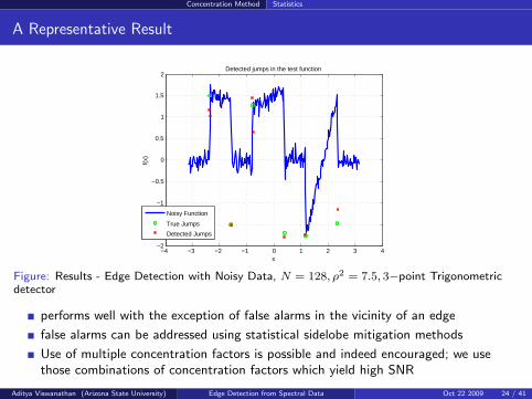
A Representative Result

−4 −3 −2 −1 0 1 2 3 4−2

−1.5

−1

−0.5

0

0.5

1

1.5

2

x

f(x)

Detected jumps in the test function

Noisy Function

True Jumps

Detected Jumps

Figure: Results - Edge Detection with Noisy Data, N = 128, ρ2 = 7.5, 3−point Trigonometricdetector

performs well with the exception of false alarms in the vicinity of an edge

false alarms can be addressed using statistical sidelobe mitigation methods

Use of multiple concentration factors is possible and indeed encouraged; we usethose combinations of concentration factors which yield high SNR


Concentration Method Iterative Formulations

In Search of Precise Jump Locations (Stefan, Viswanathan, Gelb, Renaut)

Jump approximations using the concentration method are computed using a Fourierpartial sum.

Since the jump function is piecewise-analytic, this approximation suffers fromconvergence issues.

In particular, the jump has a minimum, non-zero resolution and there are spuriousresponses in smooth regions.

Non Linear Post-processing

−3 −2 −1 0 1 2 3−1

−0.5

0

0.5

1

1.5

x

f(x)

Function

Jump function

(a) The minmod response

−3 −2 −1 0 1 2 3−1

−0.5

0

0.5

1

1.5

x

f(x)

Function

Jump function

(b) Enhancement of scales

Figure: Non-linear post-processing of the jump approximation



Problem Formulation

In setting up our iterative formulations,

We will take inspiration from sparsity enforcing regularization routines and theiriterative solutions (Tadmor and Zou).

We will exploit the characteristic responses of the concentration factors in ourproblem formulation.

We may writeSσN [f ](x) = (f ∗Kσ

N )(x) ≈ ([f ] ∗WσN )(x)

SσN [f ] is the jump approximation computed using the concentration method andconcentration factor σ(η).

WσN is the characteristic response to a unit jump using the concentration factor σ(η).

Iterative Problem Formulation

minp

‖Wp− SN [f ] ‖22 + λ‖ p ‖1

where W is a Toeplitz matrix containing shifted replicates of the characteristic response.



Representative Examples

−3 −2 −1 0 1 2 3−2

−1.5

−1

−0.5

0

0.5

1

1.5

2

x

f(x)

FunctionJump function

−3 −2 −1 0 1 2 3−1

−0.5

0

0.5

1

1.5

x

f(x)

Function

Jump function

Figure: Jump detection – Iterative Formulation (N = 40, Exponential factor)

Works well with even a small number of measurements

Works with missing coefficients and non-harmonic Fourier coefficients, i.e.,

f(ωk) :=1

2π

Z π

−πf(x)e−iωkxdx

Can be extended to blurred data (g = f ∗ h+ n) by modifying the problemformulation

minp

‖H ·W · p− SN [g] ‖22 + λ‖ p ‖1

where H is a Toeplitz matrix containing shifted replicates of the blur or psf.




−3 −2 −1 0 1 2 3−2

−1.5

−1

−0.5

0

0.5

1

1.5

2

x

f(x)

Function

Blurred function

Edges

Blur

−3 −2 −1 0 1 2 3−1

−0.5

0

0.5

1

1.5

x

f(x)

Function

Blurred function

Edges

Blur

Figure: Jump detection – Iterative Formulation (N = 128, Exponential factor, Gaussian Blur)

Works well with even a small number of measurements

Works with missing coefficients and non-harmonic Fourier coefficients, i.e.,

f(ωk) :=1

2π

Z π

−πf(x)e−iωkxdx

Can be extended to blurred data (g = f ∗ h+ n) by modifying the problemformulation

minp

‖H ·W · p− SN [g] ‖22 + λ‖ p ‖1

where H is a Toeplitz matrix containing shifted replicates of the blur or psf.


Applications

Outline

1 IntroductionMotivationProblem Statement

2 Jump detection using the Concentration methodThe Concentration MethodConcentration FactorsStatistical Analysis of the Concentration MethodIterative Formulations

3 ApplicationsPSF Estimation in Blurring ProblemsApplications to Fourier Reconstruction


Applications PSF Estimation

Convolutional Blurring (Viswanathan, Stefan, Cochran, Gelb, Renaut)

Often, the input data we observe has been subjected to a distorting physical processduring measurement, transmission or instrumentation.

A large class of these distortions can be explained using a convolutional blurringmodel.

Corrective actions often require an accurate estimate of the distortion or blur.

The convolutional blurring model can be written as

g = f ∗ h+ n

f is the true function

h is the blur or the point-spread function (psf)

n is noise

g is the observed function

Let f ∈ L2(−π, π) be piecewise-smooth. We estimate the psf starting with 2N + 1blurred Fourier coefficients g(k), k = −N, ..., N .



PSF Estimation using Edge Detection

Given the blurring modelg = f ∗ h+ n

Principle:Apply a linear edge detector. We shall assume that the edge detector can be written as aconvolution with an appropriate kernel

SσN [g] = T (f ∗ h+ n)

= (f ∗ h+ n) ∗K= f ∗ h ∗K + n ∗K= (f ∗K) ∗ h+ n ∗K≈ [f ] ∗ h+ n

Hence, we observe shifted and scaled replicates of the psf.



Example (No Noise)

−3 −2 −1 0 1 2 3−2

−1.5

−1

−0.5

0

0.5

1

1.5

2

x

f(x)

Function

(a) True function

−3 −2 −1 0 1 2 3−0.2

0

0.2

0.4

0.6

0.8

1

1.2

x

h(x)

(b) Gaussian Blur PSF

−3 −2 −1 0 1 2 3−1.5

−1

−0.5

0

0.5

1

1.5

2

x

g(x)

(c) Blurred Function

−3 −2 −1 0 1 2 3−2

−1.5

−1

−0.5

0

0.5

1

1.5

2

x

f(x)

Function

Blur after edge detection

True blur (normalized)

(d) After applying edge detection

Figure: Function subjected to Gaussian blur, N = 128



Example (No Noise)

−3 −2 −1 0 1 2 3−2

−1.5

−1

−0.5

0

0.5

1

1.5

2

x

f(x)

Function

(a) True function

−3 −2 −1 0 1 2 3−0.5

0

0.5

1

1.5

x

h(x)

(b) Motion Blur PSF

−3 −2 −1 0 1 2 3−1.5

−1

−0.5

0

0.5

1

1.5

x

g(x)

Blurred Function

(c) Blurred Function

−3 −2 −1 0 1 2 3−2

−1.5

−1

−0.5

0

0.5

1

1.5

2

x

f(x)

Function



(d) After applying edge detection

Figure: Function subjected to motion blur, N = 128




−3 −2 −1 0 1 2 3−2

−1.5

−1

−0.5

0

0.5

1

1.5

2

x

f(x)

Function

Blurred, noisy function



(a) Noisy blur estimation

−3 −2 −1 0 1 2 3−2

−1.5

−1

−0.5

0

0.5

1

1.5

2

x

f(x)

Function




(b) After low-pass filtering

Figure: Function subjected to Gaussian blur, N = 128

Noise distribution – n ∼ CN (0, 1.5(2N+1)2

)

Second picture subjected to low-pass (Gaussian) filtering

It is conceivable that the parameter estimation can take into account the effect ofGaussian filtering




−3 −2 −1 0 1 2 3−2

−1.5

−1

−0.5

0

0.5

1

1.5

2

x

f(x)

Function




(a) Noisy blur estimation

−3 −2 −1 0 1 2 3−2

−1.5

−1

−0.5

0

0.5

1

1.5

2

x

f(x)

Function




(b) After TV denoising

Figure: Function subjected to Motion blur, N = 128

Cannot perform conventional low-pass filtering since blur is piecewise-smooth

We compute the noisy blur estimate SN [g] ≈ [f ] ∗ h+ n ∗KN

Denoising problem formulation

minp

‖ p− SN [g] ‖22 + λ‖Lp ‖1

where L is a derivative matrix.


Applications Fourier Reconstruction

Fourier Reconstruction of Piecewise-smooth functions

SNf(x) =NX

k=−N

f(k)eikx, f(k) =1

2π

Z π

−πf(x)e−ikxdx

Consequences of Gibbs

Non-uniform convergence – presence of non-physical oscillations in the vicinity ofdiscontinuitiesReduced order of convergence – first order convergence even in smooth regions ofthe reconstruction

−1 −0.8 −0.6 −0.4 −0.2 0 0.2 0.4 0.6 0.8 1

−1

−0.5

0

0.5

1

1.5

2

x

SN

f(x)

Fourier Reconstruction

TrueFourier

(a) Reconstruction

−1 −0.8 −0.6 −0.4 −0.2 0 0.2 0.4 0.6 0.8 1−7

−6

−5

−4

−3

−2

−1

0

x

Log 10

|e|

Log Error in Reconstruction

(b) Reconstruction error

Figure: Gibbs Phenomenon, N = 32Aditya Viswanathan (Arizona State University) Edge Detection from Spectral Data Oct 22 2009 33 / 41


Filtered Fourier Reconstructions

Filtering helps to ameliorate the effects of Gibbs, but does not eliminate it. In fact, itintroduces a smearing artifact in the vicinity of a discontinuity.

−1 −0.8 −0.6 −0.4 −0.2 0 0.2 0.4 0.6 0.8 1

−1

−0.5

0

0.5

1

1.5

2

x

SN

f(x)

Fourier Reconstruction

TrueFourier

(a) Filtered Reconstruction

−1 −0.8 −0.6 −0.4 −0.2 0 0.2 0.4 0.6 0.8 1−16

−14

−12

−10

−8

−6

−4

−2

0

x

Log 10

|e|

Log Error in Reconstruction


Figure: Exponentially Filtered Reconstruction, p = 2, N = 64



Spectral Re-projection (Gottlieb and Shu)

Spectral re-projection schemes were formulated to resolve the Gibbs phenomenon.They involve reconstructing the function using an alternate basis, Ψ (known as aGibbs complementary basis).

Reconstruction is performed using the rapidly converging series

f(x) ≈mXl=0

clψl(x), where cl =〈fN , ψl〉w‖ψl‖2w

, fN is the Fourier expansion of f

Reconstruction is performed in each smooth interval. Hence, we require jumpdiscontinuity locations

High frequency modes of f have exponentially small contributions on the low modesin the new basis



Spectral Re-projection – An Example

−1 −0.8 −0.6 −0.4 −0.2 0 0.2 0.4 0.6 0.8 1−1

−0.5

0

0.5

1

1.5

2

x

f(x)

Gegenbauer reconstruction

(a) Reconstruction

−1 −0.8 −0.6 −0.4 −0.2 0 0.2 0.4 0.6 0.8 1−16

−14

−12

−10

−8

−6

−4

−2

x

Log

|e|

Log error

N=32

N=64

N=256


Figure: Spectral Reprojection Reconstructions



Non-harmonic Fourier Reconstruction (Viswanathan, Gelb, Cochran, Renaut)

−3 −2 −1 0 1 2 3−2

−1.5

−1

−0.5

0

0.5

1

1.5

2

x

f(x)

Function

(a) Template Function

−30 −20 −10 0 10 20 300

0.05

0.1

0.15

0.2

0.25

0.3

0.35

0.4

0.45

ω

|f(ω

)|

Fourier Transform

(b) Fourier Transform

Figure: A motivating example

Fourier samples violate the quadrature rule for discrete Fourier expansion

Computational issue – no FFT available

Mathematical issue – given these coefficients, can we/how do we reconstruct thefunction?

Resolution – what accuracy can we achieve given a finite (usually small) number ofcoefficients?



Non-harmonic Fourier Reconstruction (Viswanathan, Gelb, Cochran, Renaut)

−3 −2 −1 0 1 2 3−2

−1.5

−1

−0.5

0

0.5

1

1.5

2

x

f(x)

Function

(a) Template Function

−30 −20 −10 0 10 20 300

0.05

0.1

0.15

0.2

0.25

0.3

0.35

0.4

0.45

ωk

|f(ω

k)|

Fourier Transform

Fourier transformAcquired samples

(b) Fourier Coefficients, N = 32

Figure: A template example

Fourier samples violate the quadrature rule for discrete Fourier expansion

Computational issue – no FFT available

Mathematical issue – given these coefficients, can we/how do we reconstruct thefunction?

Resolution – what accuracy can we achieve given a finite (usually small) number ofcoefficients?



Reconstruction Procedure

1 recover equispaced coefficients f(k)

2 partial Fourier reconstruction using the FFT algorithm

Equispaced coefficients are obtained by inverting a model derived from application of thesampling theorem.

−150 −100 −50 0 50 100 1500

0.05

0.1

0.15

0.2

0.25

0.3

0.35

0.4

0.45

k

F(k

)


TrueInterpolated

(a) Recovered Fourier coeffi-cients

−150 −100 −50 0 50 100 150−15

−10

−5

0

k

Log

| E |

Error in Fourier Coefficients

(b) Error in recovered coeffi-cients

−3 −2 −1 0 1 2 3−2

−1.5

−1

−0.5

0

0.5

1

1.5

2

x

f(x)

Function Reconstruction

True

URS

(c) Filtered reconstruction

Figure: Reconstruction result, N = 128



Reconstruction Procedure

1 recover equispaced coefficients f(k)

2 partial Fourier reconstruction using the FFT algorithm

Equispaced coefficients are obtained by inverting a model derived from application of thesampling theorem.

30 40 50 60 70 80 90 100 110 120

−0.03

−0.02

−0.01

0

0.01

0.02

0.03

0.04

0.05

0.06

k

F(k

)


TrueInterpolated

(a) Recovered Fourier coeffi-cients

−150 −100 −50 0 50 100 150−15

−10

−5

0

k

Log

| E |

Error in Fourier Coefficients

(b) Error in recovered coeffi-cients

−3 −2 −1 0 1 2 3−2

−1.5

−1

−0.5

0

0.5

1

1.5

2

x

f(x)


True

URS

(c) Filtered reconstruction

Figure: Reconstruction result, N = 128



Incorporating Edge Information

Compute the high frequency modes using the relation

f(k) =Xp∈P

[f ](ζp)e−ikζp

2πik

−3 −2 −1 0 1 2 3−2

−1.5

−1

−0.5

0

0.5

1

1.5

2

x

f(x)


True

With edge information

(a) Reconstruction - Using edge informa-tion

30 40 50 60 70 80 90 100 110 120 130

−0.02

−0.01

0

0.01

0.02

0.03

kF

(k)


TrueWith edge information

(b) The high modes - Using edge infor-mation

Figure: Reconstruction of a test function using edge information


Summary

Summary

We summarized the concentration method of edge detection.

We looked at routines to design concentration factors.

We showed iterative routines for accurate detection of edges.

We briefly surveyed the statistical properties of concentration edge detection.

We looked at applications of edge detection toPoint spread function estimation in blurring problems.Fourier reconstruction of piecewise-smooth functions – spectral re-projection.Non-harmonic Fourier reconstruction.


Summary

References

Concentration Method

1 A. Gelb and E. Tadmor, Detection of Edges in Spectral Data, in Appl. Comp.Harmonic Anal., 7 (1999), pp. 101–135.

2 A. Gelb and E. Tadmor, Detection of Edges in Spectral Data II. NonlinearEnhancement, in SIAM J. Numer. Anal., Vol. 38, 4 (2000), pp. 1389–1408.

Statistical Formulation

1 A. Viswanathan, D. Cochran, A. Gelb and D. Cates, Detection of SignalDiscontinuities from Noisy Fourier Data, in Conf. Record of the 42nd Asilomar Conf.on Signals, Systems and Comp., Oct. 2008

Iterative Formulations

1 E. Tadmor and J. Zou, Novel edge detection methods for incomplete and noisyspectral data, in J. Fourier Anal. Appl., Vol. 14, 5 (2008), pp. 744–763.

Spectral Re-projection

1 D. Gottlieb and C.W. Shu, On the Gibbs phenomenon and its resolution, inSIAM Review (1997), pp. 644–668.


Edge Detection from Spectral Data With Applications to PSF … · Edge Detection from Spectral Data...

Documents

Transcript of Edge Detection from Spectral Data With Applications to PSF … · Edge Detection from Spectral Data...